University of Arkansas, FayettevilleScholarWorks@UARK

Theses and Dissertations

1-2018

Collaborative Robotic Path Planning for IndustrialSpraying Operations on Complex GeometriesSteven BrownUniversity of Arkansas, Fayetteville

Follow this and additional works at: https://scholarworks.uark.edu/etd

Part of the Artificial Intelligence and Robotics Commons, Graphics and Human ComputerInterfaces Commons, Industrial Engineering Commons, and the Robotics Commons

This Thesis is brought to you for free and open access by ScholarWorks@UARK. It has been accepted for inclusion in Theses and Dissertations by anauthorized administrator of ScholarWorks@UARK. For more information, please contact scholar@uark.edu, ccmiddle@uark.edu.

Recommended CitationBrown, Steven, "Collaborative Robotic Path Planning for Industrial Spraying Operations on Complex Geometries" (2018). Theses andDissertations. 3019.https://scholarworks.uark.edu/etd/3019

Collaborative Robotic Path Planning for Industrial Spraying Operations on Complex Geometries

A thesis submitted in partial fulfillment

of the requirements for the degree of

Master of Science in Industrial Engineering

by

Steven Louis Brown

University of Arkansas

Bachelor of Science in Industrial Engineering, 2016

December 2018

University of Arkansas

This thesis is approved for recommendation to the Graduate Council.

Harry Pierson, Ph.D.

Thesis Director

W. Art Chaovalitwongse, Ph.D. Chase Rainwater, Ph.D.

Committee Member Committee Member

ABSTRACT

Implementation of automated robotic solutions for complex tasks currently faces a few major

hurdles. For instance, lack of effective sensing and task variability – especially in high-mix/low-

volume processes – creates too much uncertainty to reliably hard-code a robotic work cell.

Current collaborative frameworks generally focus on integrating the sensing required for a

physically collaborative implementation. While this paradigm has proven effective for mitigating

uncertainty by mixing human cognitive function and fine motor skills with robotic strength and

repeatability, there are many instances where physical interaction is impractical but human

reasoning and task knowledge is still needed. The proposed framework consists of key modules

such as a path planner, path simulator, and result simulator. An integrated user interface

facilitates the operator to interact with these modules and edit the path plan before ultimately

approving the task for automatic execution by a manipulator that need not be collaborative.

Application of the collaborative framework is illustrated for a pressure washing task in a

remanufacturing environment that requires one-off path planning for each part. The framework

can also be applied to various other tasks, such as spray-painting, sandblasting, deburring,

grinding, and shot peening. Specifically, automated path planning for industrial spraying

operations offers the potential to automate surface preparation and coating in such environments.

Autonomous spray path planners in the literature have been limited to generally continuous and

convex surfaces, which is not true of most real parts. There is a need for planners that

consistently handle concavities and discontinuities, such as sharp corners, holes, protrusions or

other surface abnormalities when building a path. The path planner uses a slicing-based method

to generate path trajectories. It identifies and quantifies the importance of concavities and

surface abnormalities and whether they should be considered in the path plan by comparing the

true part geometry to the convex hull path. If necessary, the path is then adapted by adjusting the

movement speed or offset distance at individual points along the path. Which adaptive method is

more effective and the trade-offs associated with adapting the path are also considered in the

development of the path planner.

ACKNOWLEDGEMENTS

I would first like to thank Dr. Harry Pierson for his support and guidance over the past few

years, without which, I would not be where I am today. His unending passion for robotics and

automation has opened my eyes to new possibilities and inspired me throughout my research.

I would also like to thank all of the faculty and staff in the Industrial Engineering department

at the University of Arkansas who have helped me throughout the years. At this point, there are

too many to count, but I am grateful for every one of them.

I also wish to acknowledge the engineering team at Red River Army Depot for allowing me the

opportunity to pursue this idea and to study their processes.

Additionally, I would like to thank Greg Harms for his invaluable work developing the user

interface that has made all of the work I’ve done look good.

Finally, I would like to thank my family and friends for supporting me throughout the process

and being there when I need them most. I am beyond grateful for each and every one of you.

TABLE OF CONTENTS

1. INTRODUCTION ................................................................................................................................................. 1

2. A COLLABORATIVE FRAMEWORK FOR ROBOTIC TASK SPECIFICATION .......................................... 2

2.1. LITERATURE REVIEW ............................................................................................................................. 3

2.2. GENERAL FRAMEWORK DESIGN ......................................................................................................... 5

2.2.1. Path Planner ............................................................................................................................................. 8

2.2.2. Path Analysis ........................................................................................................................................... 9

2.2.3. Path Simulation and User Interface ....................................................................................................... 10

2.2.4. Path Modifier ......................................................................................................................................... 13

2.3. IMPLEMENTATION ................................................................................................................................ 14

2.4. CONCLUSIONS ........................................................................................................................................ 16

2.5. REFERENCES ........................................................................................................................................... 17

3. ADAPTIVE PATH PLANNING OF NOVEL COMPLEX PARTS FOR INDUSTRIAL SPRAYING

OPERATIONS ............................................................................................................................................................ 20

3.1. LITERATURE REVIEW ........................................................................................................................... 21

3.1.1. Path Planning ......................................................................................................................................... 21

3.1.2. Process Simulation ................................................................................................................................. 24

3.2. METHODS ................................................................................................................................................ 25

3.2.1. Tool Path Trajectory .............................................................................................................................. 27

3.2.2. Slicing the Part ....................................................................................................................................... 28

3.2.3. Path Building on the Slice ..................................................................................................................... 29

3.2.4. Full Path Concatenation ......................................................................................................................... 35

3.2.5. Partial Path Creation .............................................................................................................................. 36

3.2.6. Adaptive Methods .................................................................................................................................. 38

3.2.7. Analysis ................................................................................................................................................. 45

3.2.8. Experimental Design.............................................................................................................................. 46

3.3. RESULTS .................................................................................................................................................. 47

3.4. DISCUSSION ............................................................................................................................................ 55

3.5. CONCLUSIONS ........................................................................................................................................ 59

3.6. REFERENCES ........................................................................................................................................... 60

3.7. APPENDIX A – Test Parts ........................................................................................................................ 64

3.7.1. Part A - Test Part ................................................................................................................................... 64

3.7.2. Part B - Incidence Test ........................................................................................................................... 65

3.7.3. Part C - Solid Wheel Upright ................................................................................................................. 66

3.7.4. Part D - Blade Reduced ......................................................................................................................... 67

3.7.5. Part E - Wing Section Reduced ............................................................................................................. 68

3.8. APPENDIX B – Kernel Density Estimates ................................................................................................ 69

3.9. APPENDIX C - Histograms ....................................................................................................................... 70

3.10. APPENDIX D – Versus Plots .................................................................................................................... 72

3.11. APPENDIX E – Individual Treatment Results .......................................................................................... 74

3.11.1. Part A - Test Part ............................................................................................................................... 74

3.11.2. Part B – Incidence Test...................................................................................................................... 75

3.11.3. Part C – Solid Wheel Upright ............................................................................................................ 77

3.11.4. Part D – Blade Reduced .................................................................................................................... 79

3.11.5. Part E – Wing Section Reduced ........................................................................................................ 80

3.12. APPENDIX F – Nomenclature Table ........................................................................................................ 83

4. FINAL CONCLUSIONS..................................................................................................................................... 85

PUBLISHED PAPERS

Chapter 2: Published

S. Brown and H. A. Pierson, “A Collaborative Framework for Robotic Task

Specification,” Procedia Manufacturing, vol. 17, pp. 270–277, 2018.

Chapter 3: Abstract Under Review

S. Brown, “Adaptive Path Planning of Novel Complex Parts for Industrial Spraying

Operations.”

1

1. INTRODUCTION

When the idea for this research was first conceived, the task was to design an automated

pressure washing work cell capable of handling a large majority of the parts present at one of the

Army’s rework and rebuild depots. This presented a particular challenge due to the vast

differences in part size and geometry that needed to be cleaned on a daily basis. The facility is

responsible for cleaning pallets of smaller parts, as well as full tank bodies. Further compounding

the problem was the realization that there was almost no way of consistently identify the exact

geometry of a part. Whether that be from lack of existing data, easy to miss differences between

parts or the fact that the process is still manual and most parts are still custom made, especially

for rework and rebuild facilities like this one.

In the past, these challenges have deterred most facilities from attempting to automate the

process and choosing to do it manually instead. While this is certainly the most common method,

the physical toll these jobs take on the people doing them is undeniable and until recently the

technology needed to automate these tasks has been relatively inaccessible, whether that be due

to cost or the sheer difficulty of the task being automated. Specifically, full coverage path

planning is one of the most difficult tasks to automate reliably and economically. Not to say it

isn’t doable, but most cases where these tasks are automated don’t need to build a new path plan

for each part. They are typically used to repetitively do the same set of preprogrammed parts

over and over again.

Given the knowledge that human operators are very good at making the judgement calls of

what needs to really be cleaned and that a generally good path plan can be built on the fly by an

automated system, the task became how to blend a human’s cognitive function with the precision

and endurance of an automated robotic system, an idea pioneered by the collaborative robotics

2

community. Taking this idea a step further, adaptive path planning was embraced to create a

better path than the generally good path created by the naïve path planner. Due to the growing

scope of this project, it was broken down into two separate problems. The first being what does

the collaborative system look like from the initial input to user verification and ultimately

process execution, and the second being what does an adaptive path planner for pressure washing

look like. These two problems were answered in two separate papers and have been included as

Chapters 2 and 3 of this thesis.

2. A COLLABORATIVE FRAMEWORK FOR ROBOTIC TASK SPECIFICATION

Since the first industrial implementations of robotic solutions in manufacturing environments,

task specification has been one of the toughest and most time-consuming parts of the

implementation process. As robotics has advanced, so has the technology surrounding task

specification; however, there is still a need for the operator to physically program the robot. While

this is fine for low-mix, high-volume production processes, it is a very restrictive requirement for

the automation of lower-volume processes. Automated task specification would go a long way

toward alleviating some of the hurdles faced by high-mix, low-volume processes. However, the

implementation of automated robotic solutions for complex tasks currently faces a few major

hurdles. Lack of effective sensing and task variability create too much uncertainty to reliably hard-

code a robotic work cell. Collaborative robotics have proven effective for mitigating uncertainty

by mixing human cognitive function and fine motor skills with robotic strength and repeatability.

Yet, there are many instances where physical interaction is impractical, as human reasoning and

task knowledge are still needed. The solution is a framework that blends the latest developments

in automated task specification with the experience and cognition of a human operator to provide

a more accurate task specification. While this chapter does focus on surface finishing tasks such

3

as pressure washing, sandblasting shot peening, deburring, grinding, sanding, and wire brushing,

the framework can also be applied to any robotic task that does not have a predefined path, such

as assembly, inspection, packaging, and pick-and-place operations.

The inspiration for this chapter is a pressure washing work cell. The current work cell is an

entirely manual operation with the operators being subjected to high ergonomic risk factors [1].

As such, this process is a strong candidate for automation, but high degrees of variability and

uncertainty, combined with extremely difficult perception problems (e.g., differentiating black

paint from grease) make traditional robotic automation impractical. By designing an automated

system to suggest a toolpath for cleaning and then using the operator’s intelligence and

understanding to inform the automated side of potential changes, the system can consistently

handle the variability in the process.

2.1. LITERATURE REVIEW

While there are many well-documented methods, safety measures, and best practices for general

robotic implementations, there are few frameworks designed for the challenges and needs of

automating a specific task. The most significant research has been in a software-based approach

to connect various sensors and actuators together to create complex systems, such as robots, and

has resulted in the formation of the open-source Robotic Operating System [2]. While the ROS

consortium and others focus on the integration of tools, sensors, and some external software, other

research has focused on how robots communicate within themselves [3]. Depending on how intra-

robot communication is viewed, this can be interpreted in one of two ways: either by considering

each piece of a robot as its own robotic module or by considering a group of similar robots focused

on the same task. When considering a modular robot, there are steps that can be taken to design

the optimal robot based on the available modules and the needs of the task [4]. While this method

4

does help when deciding what style or configuration of robots is needed, it does not address

anything other than the physical requirements of the task. When considering communication across

multiple robots, there are a variety of methods being used to manage the interactions of multiple

robots, from linked pathed planners to swarm intelligence [5, 6]. This has predominately been a

focus of mobile robotics, especially with the rise of cleaning and delivery robots [7, 8]. With the

ability to control multiple robots or parts of a robot independently to accomplish a task, other

research has looked at how a distributed system might manage multiple simultaneous requests

either by prioritizing certain tasks over others or by attempting to complete multiple tasks at the

same time [9]. On the collaborative side, there are some general frameworks for how a robot could

communicate with a human, but they are focused around mobile robotics and collision avoidance

[10].

Over the past few years there has been a major push in the robotics community toward a new

style of robot that can better interact with human operators. Called collaborative robots, or cobots,

they are designed to work together with humans to accomplish a task in the most productive way

possible by leveraging the strength and endurance of robots with the flexibility and decision

making of humans [11]. They are able to do this by integrating new safety standards and methods

into this new generation of robots and by refitting systems with older industrial robots to meet the

new safety standards as discussed below. These new safety standards have allowed for numerous

new automation opportunities, both in how robots are used and where they can be used [12, 13].

Traditionally, whenever an operator needs to physically interact with a robot in any way, they

need to use a lock-out procedure to ensure that either the robot’s servos are turned off or the robot

is locked in place by some other mechanism. With safety-rated monitored stops, this is no longer

necessary. As long as the robot does not move from its current position, the operator is free to enter

5

the workspace without shutting down the robot or going through a lock-out procedure. A hand-

guided cobot allows for the operator to directly affect the position of the robot with their hands

without deactivating the servo motors. This is especially useful for robotic arms with axes that can

be easily affected by gravity and would usually require power to maintain their position. This style

of collaboration allows for faster and easier teaching and programming, and allows humans to use

the robots to lift the majority of a heavy load while the operator guides it into place. A cobot

utilizing speed and separation monitoring allows the operator to move freely throughout the

workspace while the robot is in motion, as long as a dynamically defined minimum separation

distance is maintained between the robot and the operator; otherwise, the robot will immediately

initiate a protective stop. Power- and force-limiting robots are specifically built for physical

contact with the operator that can occur both intentionally and unintentionally by limiting the

maximum capable applied forces to comply with defined threshold limits [14].

Aside from the physical interpretations of collaborative operation, there are also many human

interface changes that can make a robotic implementation collaborative. As discussed above, some

of the collaborative operating methods can be used to enhance the programming experience by

allowing the human to interact with the robot [15]. While this does not lead to a collaborative

operation, it does minimize the time spent on setting up the operation, which can be just as

valuable.

2.2. GENERAL FRAMEWORK DESIGN

This section discusses the modules required within the framework as well as reveals the key

attributes for the success of each module. Figure 1 illustrates how the individual modules interact

with each other, the external components of the system, and the human operator. From a high level,

the system takes the provided 3D data and initial user input as parameters into the path planner to

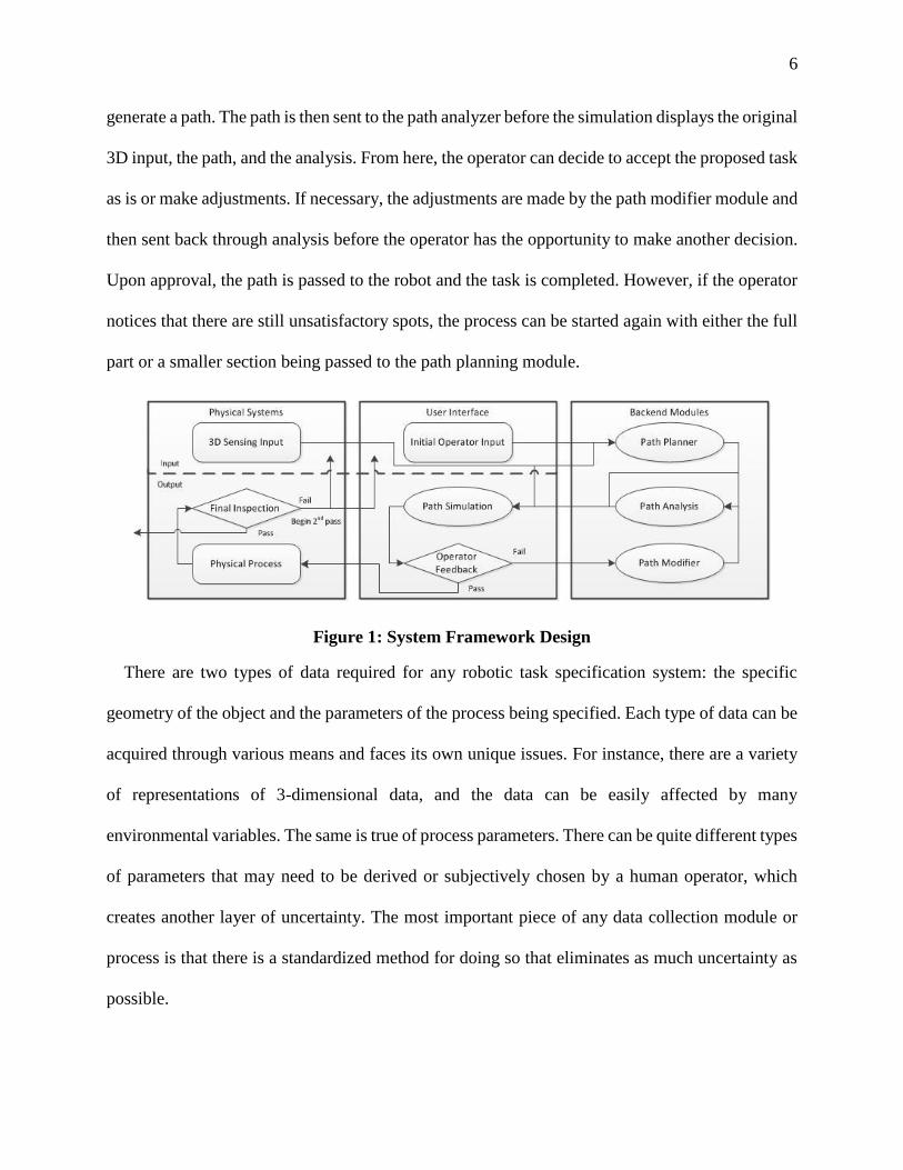
6

generate a path. The path is then sent to the path analyzer before the simulation displays the original

3D input, the path, and the analysis. From here, the operator can decide to accept the proposed task

as is or make adjustments. If necessary, the adjustments are made by the path modifier module and

then sent back through analysis before the operator has the opportunity to make another decision.

Upon approval, the path is passed to the robot and the task is completed. However, if the operator

notices that there are still unsatisfactory spots, the process can be started again with either the full

part or a smaller section being passed to the path planning module.

Figure 1: System Framework Design

There are two types of data required for any robotic task specification system: the specific

geometry of the object and the parameters of the process being specified. Each type of data can be

acquired through various means and faces its own unique issues. For instance, there are a variety

of representations of 3-dimensional data, and the data can be easily affected by many

environmental variables. The same is true of process parameters. There can be quite different types

of parameters that may need to be derived or subjectively chosen by a human operator, which

creates another layer of uncertainty. The most important piece of any data collection module or

process is that there is a standardized method for doing so that eliminates as much uncertainty as

possible.

7

One might assume that it is feasible to fully automate the process and eliminate a vast majority

of the uncertainty, but there are still some large issues surrounding 3D data collection that need to

be solved before that is possible for a one-off task specification system [16, 17]. One of the biggest

is the need to ensure that the data is completely accurate. 3D sensing technologies can still be

easily fooled due to environmental or surface conditions. Lighting plays a huge part in achieving

an accurate scan of the part. If a surface is not reflecting the light as the system expects an error

may occur in the final rendering. This could ultimately lead to collisions during the task. There is

also the possibility that the true part geometry is being obscured by dirt or debris. While this is not

problematic in processes such as pressure washing, it can cause challenges in processes such as

deburring, where debris could be interpreted as integral to the piece and thus not be removed.

Another concern is that the environment or the process itself could cause problems for the sensing

mechanism. Any spray, smoke, particles, or general debris being scattered about during the

process, along with any additional environmental variable, could obscure or alter the view of the

sensors. Covering the sensors to protect them and scanning ex situ both present issues. Not only is

it necessary to touch the part twice, but there is the concern about orientation and registration issues

once the part is placed in the workspace. Achieving the appropriate orientation and registration of

an unfixtured part with no on-site 3D sensing equipment puts a significant burden on the operator

to get things exactly right every time.

Other big concerns for the initial data collection are how to ensure that the information provided

by the operator is accurate and how to determine the right amount of human interaction required

to maintain a flexible yet accurate system. These questions are interdependent. For the right

amount of human interaction to be determined, one must understand how much the input can vary

based on human judgement and error, and how much that particular input affects the task

8

specification process. For example, orienting and registering an unfixtured part, as described

above, requires the user to match points on the part in the robot’s workspace with the same points

on the 3D model. This brings in not only error from the operator’s judgment about it being “close

enough” but also the error in the measuring device used. Finding the right balance between

accuracy and usability while maintaining operator support can be difficult. It is important to note

that while robotic automation has seen a huge surge in popularity across many industries, only

about 10 percent of manufacturing jobs have been automated [18]. Part of that is due to the fact

that many workers are less likely to accept robots that completely replace their job without any

mistakes. In fact, recent studies show that “clumsy robots” that sometimes need help or make

mistakes are better received by humans [19]. This is where collaborative systems can be most

beneficial, by allowing limited user control and feedback to inform the robot of what should be

done while maintaining a higher level of accuracy and precision.

2.2.1. Path Planner

The path planner has the largest influence on system performance, which is not surprising

considering the large amount of work that has already been done in the area. From seed and slicing

based models to advanced genetic algorithms, there are multitudes of ways to generate an initial

tool path [20, 21]. There are several key factors to consider when designing a path planning

module. First, knowing and understanding the process and its requirements is key to building an

accurate path planner. The path needed to deburr a surface must be much more precise than the

path needed to sandblast that same surface. The controls are also different. A deburring operation

needs to control which grinding tool is used and its cutting speed, whereas a sandblasting operation

needs to control the type and quantity of sand being used. The sandblasting operation would also

be more affected by the excess coverage issues, which places more significance on finding non-

9

overlapping paths. Another key consideration would be how to link parts of the path with the

corresponding area on the surface. This is essential when considering location-specific user input

and feedback. Without any way to link areas in need with specific segments, the entire path would

need to be rebuilt every time a change is needed to be made. Another staple of a good path planner

is robustness to the noise surrounding the part. Depending on the process, this can be achieved by

generalizing the original geometry or sometimes ignoring specific pieces during the planning

phase. Finally, a good path planner should take into consideration the robot’s capabilities when

building the final path. A path that may be technically feasible may not be the best path overall

due to limits on the robot’s reach, joint limits, and singularities.

2.2.2. Path Analysis

The path analysis module provides a measure of how effective the path planner was in achieving

the desired results for the process. When designing this module, there are a few key issues. Most

importantly, an accurate mathematical representation of the end effector and the process is

required. Without this, any generated feedback will be inaccurate. While there are plenty of

existing models of various processes, each model relies on input parameters unique to the

particular setup. After an accurate process model has been achieved, there should be a

methodology defined for quantifying the effect of the process on the surface. For instance, a

pressure washing model could be quantified by the cumulative energy impingement on the surface

as a function of distance and incidence angle, while a sanding operation could be quantified by the

grit of the sander and the pressure applied. These quantifications can then be used to track the

overall work done on the surface over time. This process must then be applied to the path. The

most reliable method for modeling the entire path is to discretize the path into individual points

derived from a consistent time period. After iterating through the entire path, there will be a

10

corresponding impingement value for all of the affected facets on the surface at each time value.

These values can then be summed by facet to create the total impingement value for each facet for

the entire path. These final values may then be scaled and trimmed in a way that accurately

represents the process. For instance, a pressure washing operation is typically not concerned with

overtreating a surface, and path evaluation can consider any value over a given threshold

acceptable, whereas sandblasting would require limiting the impingement values to within a

certain range. Once the impingement values have been scaled, they can be used to inform a variety

of internal and external decisions moving forward based on the requirements of the process.

2.2.3. Path Simulation and User Interface

Assuming all of the above modules are working correctly, none of them output data in a way

that is easily comprehensible by the operator, making simulation and the human-machine interface

critical. The interface and simulation should be robust enough to allow the human operator to

quickly and easily understand what is happening, and allow them to make the appropriate

judgements and adjustments. This section will discuss some guidelines for what can be included

in this module as well as some novel ways of using the data from the previous modules.

In order to provide the necessary depth of information in simulation, there are three particular

pieces of data that should be displayed. First, there should always be a properly oriented and

accurate representation of the part. This ensures that the operator knows exactly which pieces

correspond to the physical part. However, assuming the operator is using a stationary workstation,

there is a point-of-view problem, where the operator can see only part of the object. One solution

is to mount a camera on the robot and allow for visual inspection as the robot moves through the

path, which could be time consuming. Another solution is to reskin the simulated part with actual

images of the part, similar to photogrammetry, which would allow for the most accurate initial

11

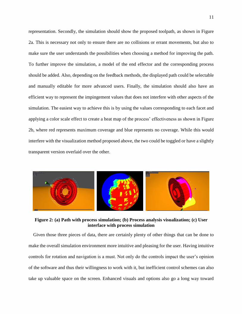
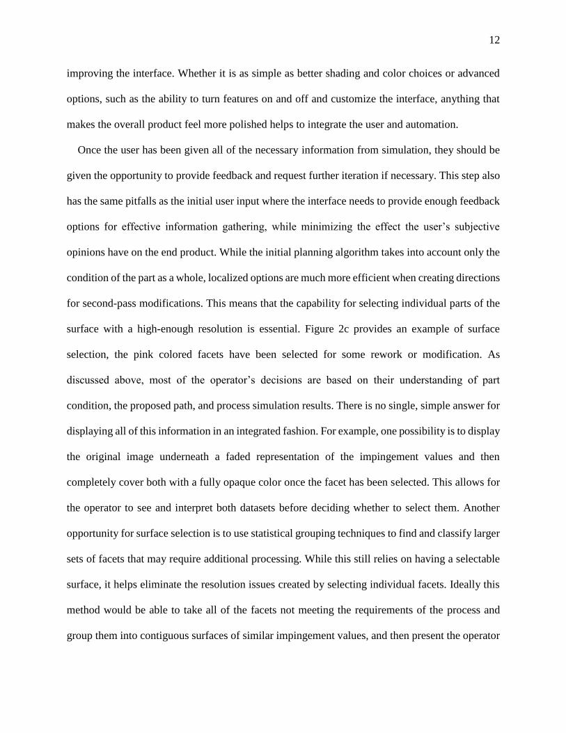
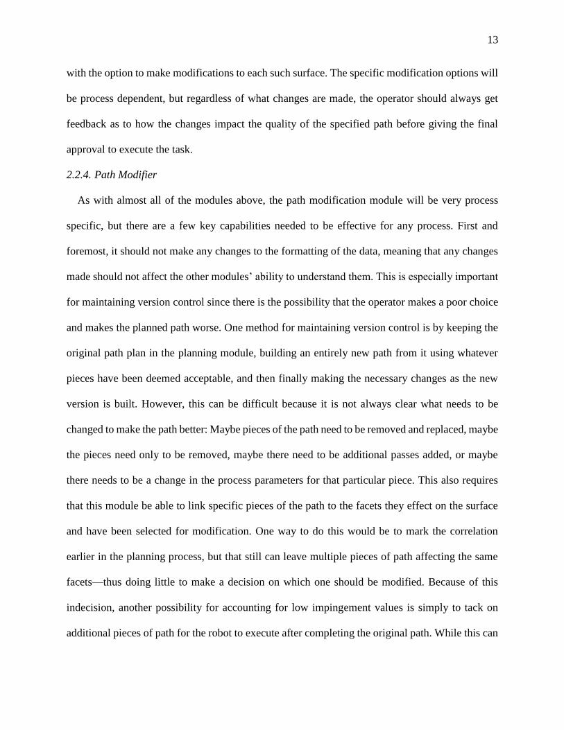
representation. Secondly, the simulation should show the proposed toolpath, as shown in Figure

2a. This is necessary not only to ensure there are no collisions or errant movements, but also to

make sure the user understands the possibilities when choosing a method for improving the path.

To further improve the simulation, a model of the end effector and the corresponding process

should be added. Also, depending on the feedback methods, the displayed path could be selectable

and manually editable for more advanced users. Finally, the simulation should also have an

efficient way to represent the impingement values that does not interfere with other aspects of the

simulation. The easiest way to achieve this is by using the values corresponding to each facet and

applying a color scale effect to create a heat map of the process’ effectiveness as shown in Figure

2b, where red represents maximum coverage and blue represents no coverage. While this would

interfere with the visualization method proposed above, the two could be toggled or have a slightly

transparent version overlaid over the other.

Figure 2: (a) Path with process simulation; (b) Process analysis visualization; (c) User

interface with process simulation

Given those three pieces of data, there are certainly plenty of other things that can be done to

make the overall simulation environment more intuitive and pleasing for the user. Having intuitive

controls for rotation and navigation is a must. Not only do the controls impact the user’s opinion

of the software and thus their willingness to work with it, but inefficient control schemes can also

take up valuable space on the screen. Enhanced visuals and options also go a long way toward

12

improving the interface. Whether it is as simple as better shading and color choices or advanced

options, such as the ability to turn features on and off and customize the interface, anything that

makes the overall product feel more polished helps to integrate the user and automation.

Once the user has been given all of the necessary information from simulation, they should be

given the opportunity to provide feedback and request further iteration if necessary. This step also

has the same pitfalls as the initial user input where the interface needs to provide enough feedback

options for effective information gathering, while minimizing the effect the user’s subjective

opinions have on the end product. While the initial planning algorithm takes into account only the

condition of the part as a whole, localized options are much more efficient when creating directions

for second-pass modifications. This means that the capability for selecting individual parts of the

surface with a high-enough resolution is essential. Figure 2c provides an example of surface

selection, the pink colored facets have been selected for some rework or modification. As

discussed above, most of the operator’s decisions are based on their understanding of part

condition, the proposed path, and process simulation results. There is no single, simple answer for

displaying all of this information in an integrated fashion. For example, one possibility is to display

the original image underneath a faded representation of the impingement values and then

completely cover both with a fully opaque color once the facet has been selected. This allows for

the operator to see and interpret both datasets before deciding whether to select them. Another

opportunity for surface selection is to use statistical grouping techniques to find and classify larger

sets of facets that may require additional processing. While this still relies on having a selectable

surface, it helps eliminate the resolution issues created by selecting individual facets. Ideally this

method would be able to take all of the facets not meeting the requirements of the process and

group them into contiguous surfaces of similar impingement values, and then present the operator

13

with the option to make modifications to each such surface. The specific modification options will

be process dependent, but regardless of what changes are made, the operator should always get

feedback as to how the changes impact the quality of the specified path before giving the final

approval to execute the task.

2.2.4. Path Modifier

As with almost all of the modules above, the path modification module will be very process

specific, but there are a few key capabilities needed to be effective for any process. First and

foremost, it should not make any changes to the formatting of the data, meaning that any changes

made should not affect the other modules’ ability to understand them. This is especially important

for maintaining version control since there is the possibility that the operator makes a poor choice

and makes the planned path worse. One method for maintaining version control is by keeping the

original path plan in the planning module, building an entirely new path from it using whatever

pieces have been deemed acceptable, and then finally making the necessary changes as the new

version is built. However, this can be difficult because it is not always clear what needs to be

changed to make the path better: Maybe pieces of the path need to be removed and replaced, maybe

the pieces need only to be removed, maybe there need to be additional passes added, or maybe

there needs to be a change in the process parameters for that particular piece. This also requires

that this module be able to link specific pieces of the path to the facets they effect on the surface

and have been selected for modification. One way to do this would be to mark the correlation

earlier in the planning process, but that still can leave multiple pieces of path affecting the same

facets—thus doing little to make a decision on which one should be modified. Because of this

indecision, another possibility for accounting for low impingement values is simply to tack on

additional pieces of path for the robot to execute after completing the original path. While this can

14

certainly work, constantly jumping from place to place means that there is a greater chance for

collisions. To combat this issue, there needs to be some collision avoidance logic built into the

path modifiers to ensure that everything will flow smoothly. Some potential modifications to the

path could include changing the attack angle, slowing down the tool head’s movement, replanning

for only the problem areas, and adjusting the offset distance for non-contact operations. At the

very least, this module should be prepared to be iterated multiple times, making the finer changes

to eventually produce a good path plan. In this case, some internal iteration might be preferred so

that the operator does not need to keep checking and rechecking all of the time.

2.3. IMPLEMENTATION

In order to realize the distributed nature of the system, the Robotic Operating System (ROS)

was used to coordinate communication amongst the nodes in the network. ROS was chosen

because it supports multiple languages and since there are no modifications to the data between

the languages. This allows a variety of sensors, hardware, software, and various other accessories

to communicate easily. It also has convenient methods for managing node executions and version

control. For example, a ROS service node holds program execution on the client side until it has

completed. This helps to ensure that the current task plan is not being modified by something else

when it is accessed by another node.

For a system like this to work, maintaining data integrity is key, especially when all of the newly

created data points need to be linked back to the originals. As discussed above, version control and

communication between languages are what ROS does well. While most languages use different

mixes of lists, arrays, tuples, and various other data structures, almost all languages hold true to

the basics such as text strings, integers, and floating-point numbers. ROS is no different, as it

supports the basic data types but uses its own structures, called messages. For this framework

15

system, custom ROS messages were written to accurately represent the data and transfer it between

the nodes, where it was translated to and from the native data structures for use.

Currently, the prototype implementation is being built on Ubuntu 16.04 with the majority of the

code written in Python 2.7. The GODOT gaming engine is used for simulation and the main user

interface. Various open-source python packages are used to handle the rest of the process. As

shown in Figure 2, the planned path is visualized along with a representation of the spraying

process. The user can then consult the impingement data as displayed on the part and select facets

needing rework. Since this is non-contact, the user can choose to modify speed or offset distance

to better clean the selected facets, and this process can then be iterated until an acceptable path is

found.

Although this chapter focuses on full-part coverage for surface-finishing task specification, the

framework can also be applied to tasks with less obvious goals, such as assembly, inspection,

packaging, and pick-and-place operations. For these tasks, many of the modules discussed are still

useful, but will have different goals and may be utilized in a different order. For the initial data

input, the system still needs to understand the pose of all objects, but the input parameters can look

different. In some cases, there may not be any input from the operator until a simulation has been

rendered. The same can be said of the path planning, analysis, and modification modules. In these

tasks, unlike full-coverage path planning, the goal may not be completely clear, since user input

could be required before anything other than a simulation of the part and environment could be

done. In these cases, an additional module could be added for identifying the task at hand and

determining what needs to go where. For instance, a task identifier module could leverage visual

and 3D data to identify where each piece fits with the other.

16

Consider an assembly robot that has been designed to help assemble a wide variety of products.

Once the system has been shown all of the parts for the assembly, a task identifier module could

make the initial decisions about what goes where before passing on those decisions to the operator

to be confirmed or edited. Once the operator gives the go-ahead, the path planner module can take

over and make a first pass at determining the appropriate trajectories for the assembly process. The

trajectories would then be reviewed by the operator who could then approve them or make edits

and suggestions for an improved trajectory. Measuring the goodness of these trajectories could be

difficult, especially when considering how to convey the results clearly to the operator, but

assembly is a bit more intuitive than finding an optimal surface covering path.

Other additional hurdles for implementing a system for non-surface finishing operations are

inevitable because there is no easy and reliable way to fully complete the entire task in simulation

before executing. For example, the above assembly trajectories rely on the gripper being able to

replicate the grip that was achieved in simulation for the rest of the trajectory to be accurate. An

alternative to this problem would be to rescan and replan each step after the robot picks up a piece

with its gripper. While this would help increase accuracy, it would add significant time to the

process. This also means that the operator needs to keep checking on the simulation throughout

the assembly process, which makes the human more of a tele-operator than a supervisor. While

that is not necessarily a bad thing and could even be ideal in some industries, it does not do much

to improve the operator’s efficiency.

2.4. CONCLUSIONS

As robotic technologies continue to advance, so should the way humans can interact with them.

Collaborative robotics both physically and virtually are the next step in furthering the integration

of robotics into industry and our everyday lives. While it is impossible to know what new

17

technologies might dramatically shift how we think about robotic implementations in the future,

having a framework for collaboration between robots and humans to complete complex and

diverse tasks will be essential. The collaborative robotic framework for task specification proposed

here is one step toward fully automated systems capable of very high-mix, low-volume

manufacturing.

2.5. REFERENCES

[1] A. Woods and H. Pierson, "Developing an Ergonomic Model and Automation Justification

for Spraying Operations," in Proceedings of the 2018 Institute of Industrial and Systems

Engineers Annual Conference, Orlando, FL, 2018.

[2] M. Quigley, B. Gerkey, K. Conley, J. Faust, T. Foote, J. Leibs, E. Berger, R. Wheeler and

A. Ng, "ROS: an open-source Robot Operating System".

[3] R. Johansson, A. Robertsson, K. Nilsson, T. Brogard, P. Cederberg, M. Olsson, T. Olsson

and G. Bolmsjo, "Sensor integration in task-level programming and industrial robotic task

execution control," Industrial Robot: An International Journal , vol. 31, pp. 284-296, 2004.

[4] Z. M. Bi and W. J. Zhang, "Concurrent Optimal Design of Modular Robotic

Configuration," Journal of Robotic Systems , vol. 18, pp. 77-87, 2001.

[5] M. Montemerlo and S. Thrun, FastSLAM: A Scalable Method for the Simultaneous

Localization and Mapping Problem in Robotics, Springer, 2007.

[6] G. Beni and J. Wang, "Theoretical Problems for the Realization of Distributed Robotic

Systems," in IEEE International Conference on Robotics and Autanatioo, Sacremento, CA,

1991.

[7] E. Prassler, A. Ritter, C. Schaeffer and P. Fiorini, "A Short History of Cleaning Robots,"

Autonomous Robots , vol. 9, pp. 211-226, 2000.

[8] A. Martinoli, K. Easton and W. Agassounon, "Modeling Swarm Robotic Systems: A Case

Study in Collaborative Distributed Manipulation," The International Journal of Robotics

Research , vol. 23, pp. 415-436, 2004.

18

[9] B. Siciliano and J.-J. E. Slotine, "A general framework for managing multiple tasks in

highly redundant robotic systems," in Fifth International Conference on Advanced

Robotics, 1991.

[10] T. Fong, C. Thorpe and C. Baur, "Collaborative Control: A Robot-Centric Model for

Vehicle Teleoperation," AAAI, 1999.

[11] A. Djuric, R. J. Urbanic and J. L. Rickli, "A Framework for Collaborative Robot (CoBot)

Integration in Advanced Manufacturing Systems".

[12] T. Anandan, "Robotic Industry Insights: Collaborative Robots and Safety," Robotic

Inustries Association, 26 Jan 2016. [Online]. Available: https://www.robotics.org/content-

detail.cfm?content_id=5908.

[13] P. Waurzyniak, "Putting Safety First in Robotic Automation," Manufacturing Engineering,

pp. 61-66, September 2016.

[14] S. Brown, A. Woods, H. Pierson and G. Parnell, "An Operations Management Perspective

on Collaborative Robotics," in American Society for Engineering Management

International Annual Conference, Huntsville, AL, 2017.

[15] Robotiq, "Teaching Robots Welding," [Online]. Available:

http://robotiq.com/solutions/robot-teaching/. [Accessed 6 May 2017].

[16] F. Remondino and S. El-Hakim, "IMAGE-BASED 3D MODELLING: A REVIEW," The

Photogrammetric Record, vol. 21, pp. 269-291, 2006.

[17] J. D. Schutter, T. D. Laet, J. Rutgeerts, W. Decré, R. Smits, E. Aertbeliën, K. Claes and H.

Bruyninckx, "Constraint-based Task Specification and Estimation for Sensor-Based Robot

Systems in the Presence of Geometric Uncertainty," The International Journal of Robotics

Research, vol. 26, pp. 433-455, 2007.

[18] H. Sirkin, M. Zinser and J. Rose, "The Robotics Revolution: The Next Great Leap in

Manufacturing," BCG, 2015. [Online]. Available:

https://www.bcg.com/publications/2015/lean-manufacturing-innovation-robotics-

revolution-next-great-leap-manufacturing.aspx.

[19] N. Mirnig, G. Stollnberger, M. Miksch, S. Stadler, M. Giuliani and M. Tscheligi, "To Err Is

Robot: How Humans Assess and Act toward an Erroneous Social Robot," Frontiers in

Robotics and AI, vol. 4, p. 21, 2017.

19

[20] W. Chen and D. Zhao, "Path Planning for Spray Painting Robot of Workpiece Surfaces,"

Mathematical Problems in Engineering, 2013.

[21] A. UGUR, "Path planning on a cuboid using genetic algorithms," Information Sciences,

vol. 178, pp. 3275-3287, 2007.

20

3. ADAPTIVE PATH PLANNING OF NOVEL COMPLEX PARTS FOR INDUSTRIAL

SPRAYING OPERATIONS

Operations such as spray painting, powder coating, pressure washing and blasting operations

make up one of the more common processes in manufacturing across many different industries.

When performed by humans, these tasks often require full body safety equipment such as coveralls

and face masks, which while they do help combat the safety issues, they can also hinder an

operator’s ability to work in the environment. For example, in a detergent based pressure washing

cell, the operator is subjected to a very hot and humid environment, which translates to a very hot

and uncomfortable suit, with spray from the pressure washing obscuring their vision through the

mask. The operator’s solution to these new problems is commonly to remove their safety

equipment. A robotic solution helps bring human operators out of what can be a very dull, dirty

and often dangerous environment, especially when considering the ergonomic impact the job can

have on a person [1].

While there are a variety of current robotic solutions in use, most only deal with parts of known

geometry or place restrictions on the types of geometries that can be serviced. This is especially

true in high-volume, low-mix production setting where the part-to-part variance is insignificant.

For these instances, quality autonomous path planning is not as critical because the path can be

fixed by the operator before execution. This method is impractical for high-mix, low-volume

processes, which are becoming more and more prevalent as large manufacturers try to meet the

needs of a wider consumer base while maintaining or increasing their efficiency and smaller

manufacturers begin to embrace automation as a viable option.

Automated full coverage path planning is nothing new and has been the focus of many research

studies. However, there is a lack of depth with regards to dealing with discontinuities, especially

21

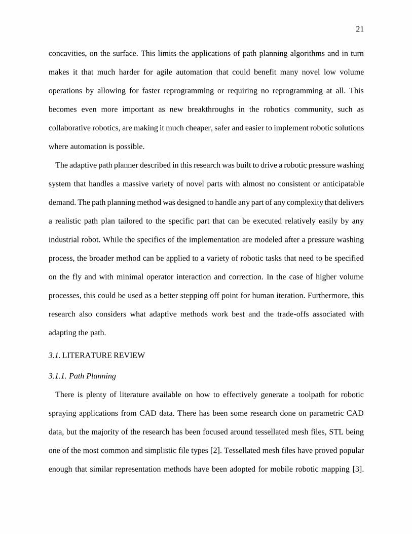
concavities, on the surface. This limits the applications of path planning algorithms and in turn

makes it that much harder for agile automation that could benefit many novel low volume

operations by allowing for faster reprogramming or requiring no reprogramming at all. This

becomes even more important as new breakthroughs in the robotics community, such as

collaborative robotics, are making it much cheaper, safer and easier to implement robotic solutions

where automation is possible.

The adaptive path planner described in this research was built to drive a robotic pressure washing

system that handles a massive variety of novel parts with almost no consistent or anticipatable

demand. The path planning method was designed to handle any part of any complexity that delivers

a realistic path plan tailored to the specific part that can be executed relatively easily by any

industrial robot. While the specifics of the implementation are modeled after a pressure washing

process, the broader method can be applied to a variety of robotic tasks that need to be specified

on the fly and with minimal operator interaction and correction. In the case of higher volume

processes, this could be used as a better stepping off point for human iteration. Furthermore, this

research also considers what adaptive methods work best and the trade-offs associated with

adapting the path.

3.1. LITERATURE REVIEW

3.1.1. Path Planning

There is plenty of literature available on how to effectively generate a toolpath for robotic

spraying applications from CAD data. There has been some research done on parametric CAD

data, but the majority of the research has been focused around tessellated mesh files, STL being

one of the most common and simplistic file types [2]. Tessellated mesh files have proved popular

enough that similar representation methods have been adopted for mobile robotic mapping [3].

22

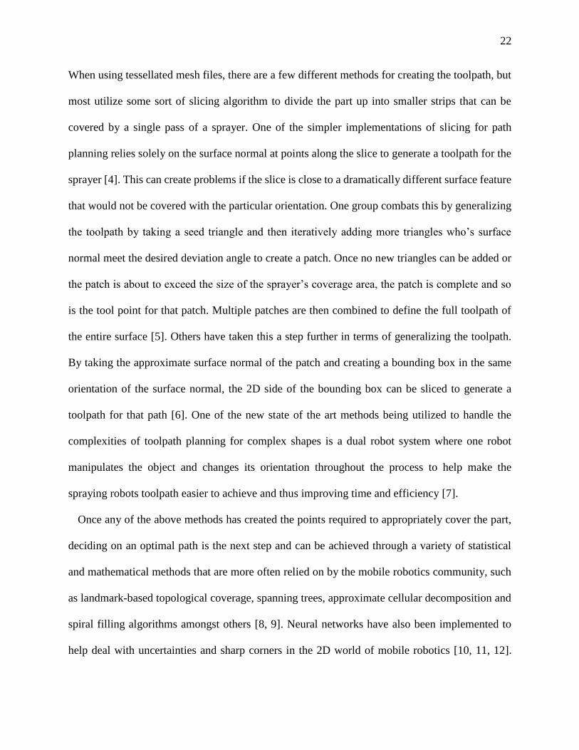
When using tessellated mesh files, there are a few different methods for creating the toolpath, but

most utilize some sort of slicing algorithm to divide the part up into smaller strips that can be

covered by a single pass of a sprayer. One of the simpler implementations of slicing for path

planning relies solely on the surface normal at points along the slice to generate a toolpath for the

sprayer [4]. This can create problems if the slice is close to a dramatically different surface feature

that would not be covered with the particular orientation. One group combats this by generalizing

the toolpath by taking a seed triangle and then iteratively adding more triangles who’s surface

normal meet the desired deviation angle to create a patch. Once no new triangles can be added or

the patch is about to exceed the size of the sprayer’s coverage area, the patch is complete and so

is the tool point for that patch. Multiple patches are then combined to define the full toolpath of

the entire surface [5]. Others have taken this a step further in terms of generalizing the toolpath.

By taking the approximate surface normal of the patch and creating a bounding box in the same

orientation of the surface normal, the 2D side of the bounding box can be sliced to generate a

toolpath for that path [6]. One of the new state of the art methods being utilized to handle the

complexities of toolpath planning for complex shapes is a dual robot system where one robot

manipulates the object and changes its orientation throughout the process to help make the

spraying robots toolpath easier to achieve and thus improving time and efficiency [7].

Once any of the above methods has created the points required to appropriately cover the part,

deciding on an optimal path is the next step and can be achieved through a variety of statistical

and mathematical methods that are more often relied on by the mobile robotics community, such

as landmark-based topological coverage, spanning trees, approximate cellular decomposition and

spiral filling algorithms amongst others [8, 9]. Neural networks have also been implemented to

help deal with uncertainties and sharp corners in the 2D world of mobile robotics [10, 11, 12].

23

While there isn’t as much of a precedent for these techniques in single use path planning, a system

that sees enough of the same or similar parts could do very well. Alternatively, genetic algorithms

have been used to solve 3D problems similar to the traveling salesman problem created by the

toolpath points [13]. As far as adaptive planning methods go, there has been plenty of research

done on mobile robotic navigation and multi-robot collision avoidance [14, 15]. However, the

research focused on the actual path is mostly focused around probabilistic roadmap planners,

which do return the best path to cover all of the defined nodes, but they do not consider the consider

the process being modeled or how changes to the path may affect the results [16].

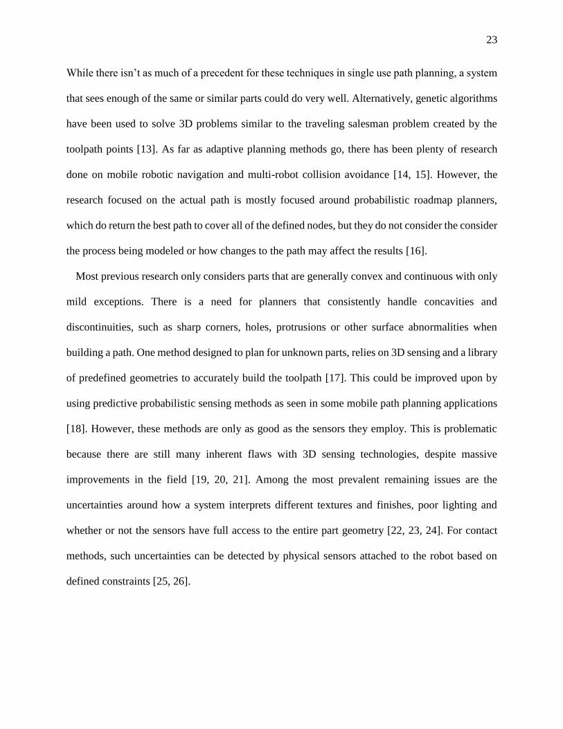
Most previous research only considers parts that are generally convex and continuous with only

mild exceptions. There is a need for planners that consistently handle concavities and

discontinuities, such as sharp corners, holes, protrusions or other surface abnormalities when

building a path. One method designed to plan for unknown parts, relies on 3D sensing and a library

of predefined geometries to accurately build the toolpath [17]. This could be improved upon by

using predictive probabilistic sensing methods as seen in some mobile path planning applications

[18]. However, these methods are only as good as the sensors they employ. This is problematic

because there are still many inherent flaws with 3D sensing technologies, despite massive

improvements in the field [19, 20, 21]. Among the most prevalent remaining issues are the

uncertainties around how a system interprets different textures and finishes, poor lighting and

whether or not the sensors have full access to the entire part geometry [22, 23, 24]. For contact

methods, such uncertainties can be detected by physical sensors attached to the robot based on

defined constraints [25, 26].

24

3.1.2. Process Simulation

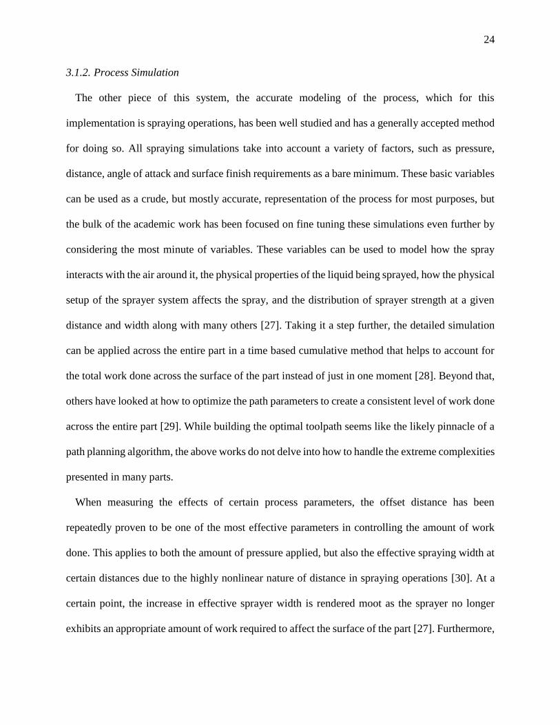
The other piece of this system, the accurate modeling of the process, which for this

implementation is spraying operations, has been well studied and has a generally accepted method

for doing so. All spraying simulations take into account a variety of factors, such as pressure,

distance, angle of attack and surface finish requirements as a bare minimum. These basic variables

can be used as a crude, but mostly accurate, representation of the process for most purposes, but

the bulk of the academic work has been focused on fine tuning these simulations even further by

considering the most minute of variables. These variables can be used to model how the spray

interacts with the air around it, the physical properties of the liquid being sprayed, how the physical

setup of the sprayer system affects the spray, and the distribution of sprayer strength at a given

distance and width along with many others [27]. Taking it a step further, the detailed simulation

can be applied across the entire part in a time based cumulative method that helps to account for

the total work done across the surface of the part instead of just in one moment [28]. Beyond that,

others have looked at how to optimize the path parameters to create a consistent level of work done

across the entire part [29]. While building the optimal toolpath seems like the likely pinnacle of a

path planning algorithm, the above works do not delve into how to handle the extreme complexities

presented in many parts.

When measuring the effects of certain process parameters, the offset distance has been

repeatedly proven to be one of the most effective parameters in controlling the amount of work

done. This applies to both the amount of pressure applied, but also the effective spraying width at

certain distances due to the highly nonlinear nature of distance in spraying operations [30]. At a

certain point, the increase in effective sprayer width is rendered moot as the sprayer no longer

exhibits an appropriate amount of work required to affect the surface of the part [27]. Furthermore,

25

with regards to time applied, there will eventually be a steady state achieved where the part can

still be within the effective range of the sprayer, but no more cumulative work can be achieved

despite multiple passes [31]. With this in mind, this research will only consider time if distance

has been adapted and more work still needs to be done.

3.2. METHODS

This approach involves taking some initial 3D data, given as an STL file in this case because the

algorithm requires normal vector, and building a convex hull around it to eliminate the collision

and accessibility issues created by non-continuous and concave surfaces. However, given a method

for determining normal vectors and building a tessellated mesh from a point cloud, any number of

3D data gathering methods could be used. At this point, the mesh is converted into a point cloud

where the centroid of each facet is linked to the normal vector of that facet. The path is then built

based on the convex hull using a slicing based method that relies on the following input parameters:

a rotation axis and the degrees of rotation, which serve to modify the slicing direction, as it is

unlikely that the part will actually be moved if the scanner is calibrated and registered correctly;

and a slice thickness, an offset distance, and an overlap percentage, which serve to quantify how

much work will be applied to the part. Once the path has been built, the points from the original

mesh, now represented as a point cloud, are mapped to specific segments of the path. In some

cases, a point can be mapped to multiple segments. The individual segments of the path are then

adapted based on the points mapped to each segment. The adaptive phase considers the true

geometry and will either modify the path to be closer to the part or it will slow the end effector

down to facilitate more cleaning power applied to a particular area. From an experimental point of

view, the system was used to test two factors; the type of adaptive algorithm used and the statistical

aggregation method used within the adaptive algorithm. The user can choose between a time

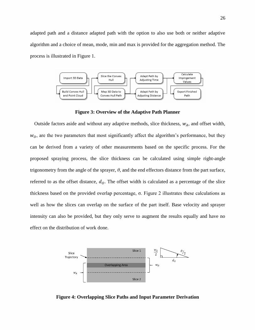
26

adapted path and a distance adapted path with the option to also use both or neither adaptive

algorithm and a choice of mean, mode, min and max is provided for the aggregation method. The

process is illustrated in Figure 1.

Figure 3: Overview of the Adaptive Path Planner

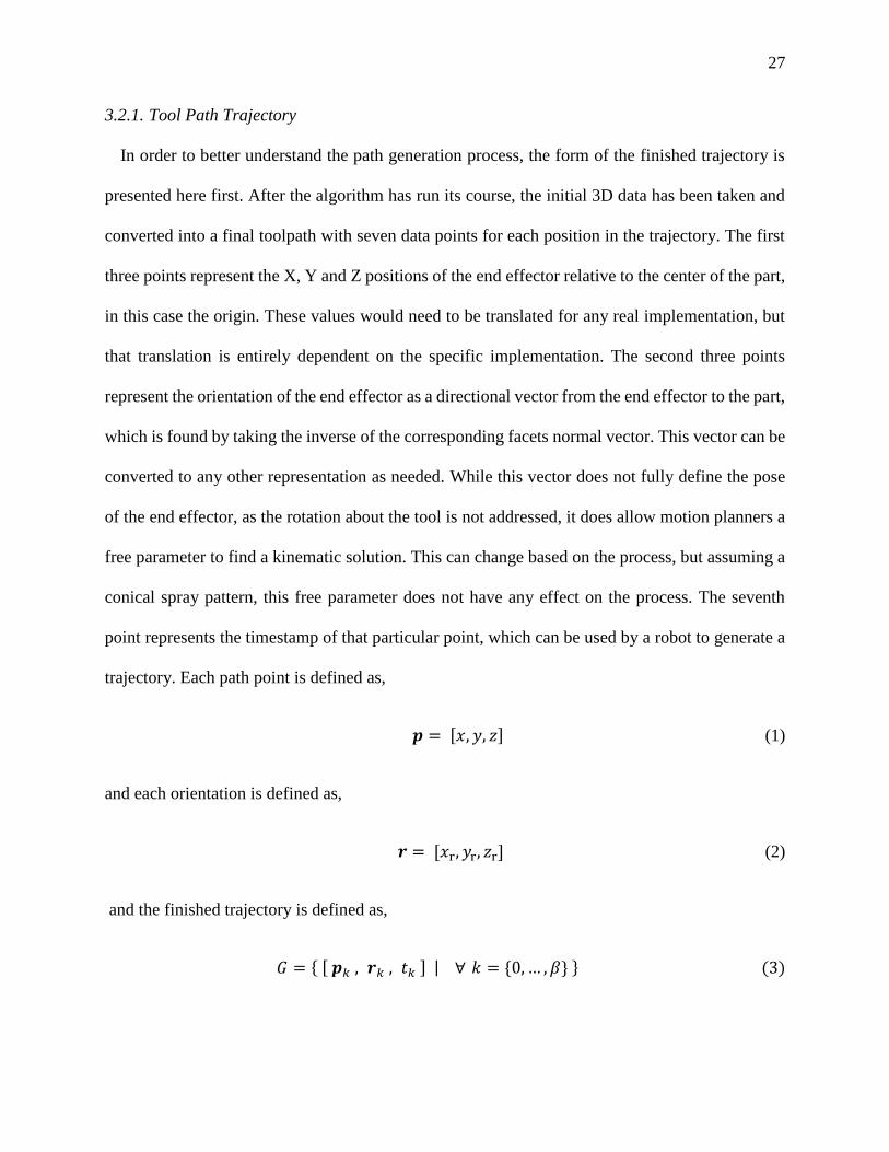
Outside factors aside and without any adaptive methods, slice thickness, 𝑤𝐴, and offset width,

𝑤𝑂, are the two parameters that most significantly affect the algorithm’s performance, but they

can be derived from a variety of other measurements based on the specific process. For the

proposed spraying process, the slice thickness can be calculated using simple right-angle

trigonometry from the angle of the sprayer, θ, and the end effectors distance from the part surface,

referred to as the offset distance, 𝑑𝑂. The offset width is calculated as a percentage of the slice

thickness based on the provided overlap percentage, σ. Figure 2 illustrates these calculations as

well as how the slices can overlap on the surface of the part itself. Base velocity and sprayer

intensity can also be provided, but they only serve to augment the results equally and have no

effect on the distribution of work done.

Figure 4: Overlapping Slice Paths and Input Parameter Derivation

27

3.2.1. Tool Path Trajectory

In order to better understand the path generation process, the form of the finished trajectory is

presented here first. After the algorithm has run its course, the initial 3D data has been taken and

converted into a final toolpath with seven data points for each position in the trajectory. The first

three points represent the X, Y and Z positions of the end effector relative to the center of the part,

in this case the origin. These values would need to be translated for any real implementation, but

that translation is entirely dependent on the specific implementation. The second three points

represent the orientation of the end effector as a directional vector from the end effector to the part,

which is found by taking the inverse of the corresponding facets normal vector. This vector can be

converted to any other representation as needed. While this vector does not fully define the pose

of the end effector, as the rotation about the tool is not addressed, it does allow motion planners a

free parameter to find a kinematic solution. This can change based on the process, but assuming a

conical spray pattern, this free parameter does not have any effect on the process. The seventh

point represents the timestamp of that particular point, which can be used by a robot to generate a

trajectory. Each path point is defined as,

𝒑 = [𝑥, 𝑦, 𝑧] (1)

and each orientation is defined as,

𝒓 = [𝑥r, 𝑦r, 𝑧r] (2)

and the finished trajectory is defined as,

𝐺 = { [ 𝒑𝑘 , 𝒓𝑘 , 𝑡𝑘 ] | ∀ 𝑘 = {0,… , 𝛽} } (3)

28

where β is the number of observations in G, P, R and T, P is the ordered set of all path points p,

R is the ordered set of all orientation vectors r, and T is the ordered set of all time values t.

3.2.2. Slicing the Part

The algorithm builds the path in a similar fashion to additive manufacturing processes. The main

difference is that when an additive manufacturing process slices a part, it is slicing to build a solid

piece, which needs many thin slices with an interior raster pattern, whereas this process is slicing

for exterior surface coverage, which uses a few thick slices without the interior raster pattern, just

the exterior perimeter. Throughout this process, all of the slicing and path building action are taken

with regards to the convex hull of the part. The original part data is used to inform the adaptive

algorithms and all analysis is done using the original part as well. The appropriate number of slices

for the convex hull is defined as,

𝑚 = ⌈(𝑍max − 𝑍min) 𝑤O⁄ ⌉ (4)

where 𝑍𝑚𝑎𝑥 and 𝑍𝑚𝑖𝑛 are the extreme values in the Z axis of the part and 𝑤𝑂 is the offset width.

The offset width, which represents the distance between each slice, is redefined so that the slices

are equally spaced along the entire part, which can be defined as,

𝑤O = (𝑍max − 𝑍min) 𝑚⁄ (5)

This ensures that there is total coverage of the part and can be modified to create overlap on the

edges of the part if necessary. The height ℎ𝑠 of each slice s is defined as,

ℎ𝑠 = 𝑍max −𝑤O

2− 𝑠𝑤O ∀ 𝑠 = {0,⋯ ,𝑚} (6)

29

where s is the slice index and 𝑤O

2 represents the offset needed to shift the slice from the edge to the

center of that slice. For each slice, s, the process described in the following sections is repeated

until all slices have been planned for and the slices are combined into one complete path.

3.2.3. Path Building on the Slice

Within each slice, which are represented as planes defined by 𝑍 = ℎ𝑠, the intersecting facets

𝐹𝑠 of the convex hull H are found by,

𝐹𝑠 = {𝑓 | 𝑢𝑓 = 1 𝑜𝑟 𝑢𝑓 = 2 } ∀ 𝑓 ∈ 𝐻 (7)

where uf is the number of vertices above the slicing plane defined by,

𝑢𝑓 = ∑ {1 , 𝒒𝑓𝑖𝑍 ≥ ℎ𝑠

0 , 𝒒𝑓𝑖𝑍 < ℎ𝑠 }3

𝑖=1 ∀ 𝑓 ∈ 𝐻 (8)

where 𝒒𝑓𝑖𝑍 is the Z value of vertex i of facet f on the convex hull H and ℎ𝑠 is the height of slice s.

If a facet has one vertex above or below the plane and the other two are on the opposite side it is

considered to be an intersecting facet and is included in the set. When a facet is sliced directly on

a single vertex, it is included as is and the following interpolation is not necessary.

When a facet is sliced, there are two intersecting points 𝒂𝑓𝑖 along the border of the facet that can

be interpolated as illustrated in Figure 3. These interpolated points are defined as,

𝒂𝑓𝑖 = 𝒒𝑓𝐴 − 𝑒𝑓𝑖𝝓𝑓𝑖 ∀ 𝑓 ∈ 𝐹𝑠𝑖 = {1,2}

(9)

where 𝒒𝑓𝐴𝑖 is the lone vertex on one side of the slicing plane, the interpolation percentage is

defined as,

30

𝑒𝑓𝑖 =(𝒒𝑓𝐴𝑍− ℎ𝑠)

𝜙𝑓𝑖𝑍 (10)

and the vector between the lone vertex and the other two vertices 𝝓𝑓𝑖 is defined as,

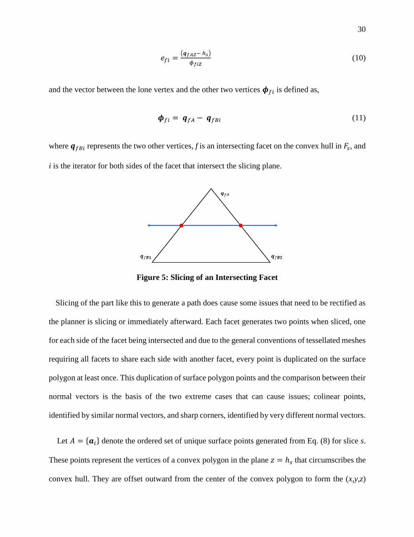
𝝓𝑓𝑖 = 𝒒𝑓𝐴 − 𝒒𝑓𝐵𝑖 (11)

where 𝒒𝑓𝐵𝑖 represents the two other vertices, f is an intersecting facet on the convex hull in 𝐹𝑠, and

i is the iterator for both sides of the facet that intersect the slicing plane.

Figure 5: Slicing of an Intersecting Facet

Slicing of the part like this to generate a path does cause some issues that need to be rectified as

the planner is slicing or immediately afterward. Each facet generates two points when sliced, one

for each side of the facet being intersected and due to the general conventions of tessellated meshes

requiring all facets to share each side with another facet, every point is duplicated on the surface

polygon at least once. This duplication of surface polygon points and the comparison between their

normal vectors is the basis of the two extreme cases that can cause issues; colinear points,

identified by similar normal vectors, and sharp corners, identified by very different normal vectors.

Let 𝐴 = {𝒂𝑖} denote the ordered set of unique surface points generated from Eq. (8) for slice s.

These points represent the vertices of a convex polygon in the plane 𝑧 = ℎ𝑠 that circumscribes the

convex hull. They are offset outward from the center of the convex polygon to form the (x,y,z)

31

elements of the tool path for the slice, 𝑃𝑠, as illustrated in Figure 4. Let 𝑁𝑖 = {�̂�𝑗} be the set of

unique normal vectors associated with the convex hull facets adjacent to ai. The offset path for the

slice, 𝑃𝑠, is then defined as,

𝑃𝑠 = {𝒑𝑘|𝒑𝑘 = 𝒂𝑖 + 𝑑o�̂�𝑗 ∀ 𝑖, 𝑗} (12)

When defining 𝑁𝑖 to be a set of unique vectors, the two cases mentioned above need to be dealt

with. These cases can be identified by looking at the dot product of the two vectors as,

{|(𝒏𝒋 ∙ 𝒏𝑗+1) − 1| ≤ 𝜺, Duplicate Points − See Equation 14

|(𝒏𝑗 ∙ 𝒏𝑗+1) − 1| > 𝜺, Sharp Corner − See Equation 15 − 17} (13)

where 𝜺 is a value between 0 and 2, which map to 0° and 180° respectively, that represents the

limit of deviation between two normal vectors. In this research, 𝜺 = 0.05, which is approximately

4.5°. For duplicate points, the resulting normal vector is defined as,

𝑁𝑖 = {�̂�𝑛𝑒𝑤 | 𝒏𝑛𝑒𝑤 = 𝒏𝑗 + 𝒏𝑗+1} (14)

This returns a single vector, �̂�𝑛𝑒𝑤, that represents the average of the normal vectors, which is

necessary because similar, but not absolutely identical normal vectors are considered unique.

In the case that the shared points have very different normal vectors there is some concern that

the resulting toolpath will cut corners and not maintain a very accurate offset distance. To alleviate

this issue, intermediary points can be added to the path to help smooth the curve and ease the strain

on the robot if the original path requires a drastic change in orientation. The set of normal vectors

is then redefined as,

𝑁𝑖 = {�̂�l | �̂�𝑙 = 𝒏𝑗 +𝑙

𝑚(�̂�𝑗+1 − �̂�𝑗) , 𝑙 = {0,… ,𝑚} } (15)

32

where �̂�𝑙 is the new normal generated for intermediary point l between normals �̂�𝑗 and �̂�𝑗+1 , and

𝑚 is the number of segments needed to meet the limit 𝜀 and is defined as,

𝑚 = ⌈|(𝒏𝑗 ∙ 𝒏𝑗+1) − 1| 𝜀⁄ ⌉ (16)

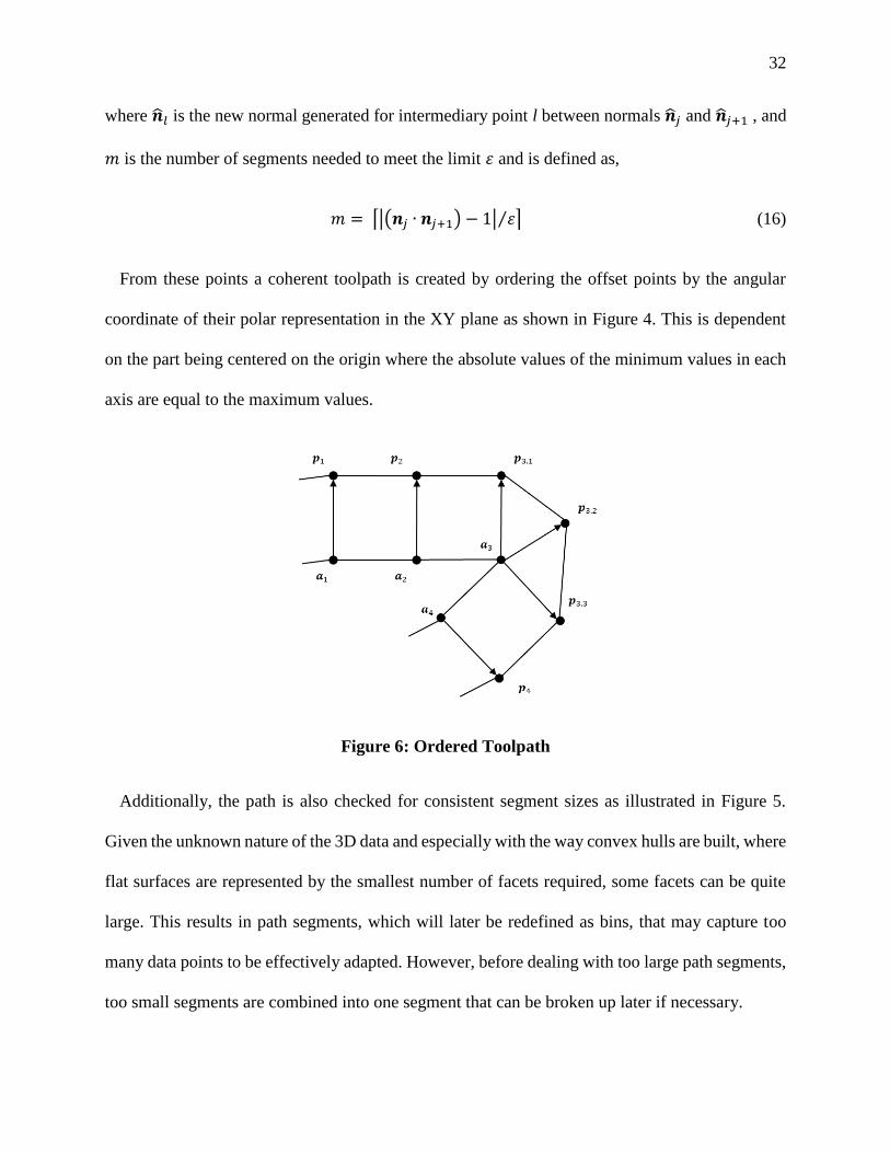
From these points a coherent toolpath is created by ordering the offset points by the angular

coordinate of their polar representation in the XY plane as shown in Figure 4. This is dependent

on the part being centered on the origin where the absolute values of the minimum values in each

axis are equal to the maximum values.

Figure 6: Ordered Toolpath

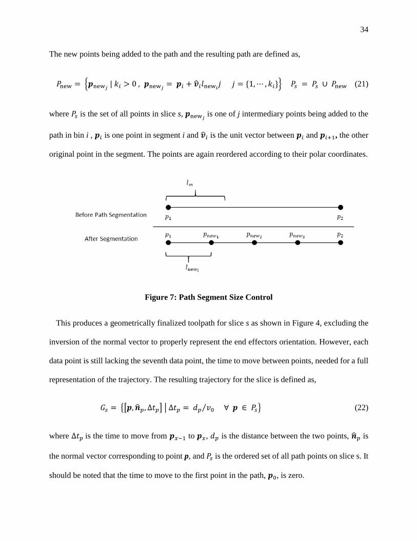
Additionally, the path is also checked for consistent segment sizes as illustrated in Figure 5.

Given the unknown nature of the 3D data and especially with the way convex hulls are built, where

flat surfaces are represented by the smallest number of facets required, some facets can be quite

large. This results in path segments, which will later be redefined as bins, that may capture too

many data points to be effectively adapted. However, before dealing with too large path segments,

too small segments are combined into one segment that can be broken up later if necessary.

33

Let Φ𝑠 = {[𝒑𝑘, �̂�𝑘]} denote the ordered set of all points and their corresponding normal vectors

in the path for slice s. Let Ξ𝑘 = {𝜑𝑗} denote the set of consecutive adjacent points that are colinear

to point 𝒑𝑘, which includes 𝜑𝑘. These colinear points can be defined in the same manner as the

duplicate points in Equation 13. If there are more than two colinear points, since any two points

are colinear, all of these points are removed from the path and two new points with new normal

vectors are defined as,

Φnew = {𝜑first𝑘 | 𝜑first𝑘 = [𝒑first𝜉

, �̂�𝜉]

𝜑last𝑘 | 𝜑last𝑘 = [𝒑last𝜉 , �̂�𝜉]

∀ 𝑘} (17)

where 𝒑first𝜉 is the first colinear point in the colinear set 𝜉, 𝒑last𝜉

is the last colinear point in 𝜉,

and �̂�𝜉 is the average normal vector of all points in 𝜉, which is defined as,

�̂�𝜉 = ∑ �̂�𝑗 ∀ 𝑗 (18)

where �̂�𝑗 is the normal vector of pair 𝜑𝑗 in the set Ξ𝑘.

When breaking larger segments down to the appropriate size, the number of segments in the

slice is defined as one less than the number of points in the path and the iterator i ranges from 0 to

the number. Segment sizes are checked and the number of additional points needed for segment i

is defined as,

𝑘𝑖 = ⌊𝑙𝑖

𝑙m⌋ (19)

where 𝑙𝑖 is the actual length of segment i and 𝑙𝑚 is the maximum allowable length. The new

segment length resulting from the additional points is defined as,

𝑙new𝑖=

𝑙𝑖

𝑘𝑖+1 (20)

34

The new points being added to the path and the resulting path are defined as,

𝑃new = {𝒑new𝑗 | 𝑘𝑖 > 0 , 𝒑new𝑗

= 𝒑𝑖 + �̂�𝑖𝑙new𝑖𝑗 𝑗 = {1,⋯ , 𝑘𝑖}} 𝑃𝑠 = 𝑃𝑠 ∪ 𝑃new (21)

where 𝑃𝑠 is the set of all points in slice s, 𝒑new𝑗 is one of j intermediary points being added to the

path in bin i , 𝒑𝑖 is one point in segment i and �̂�𝑖 is the unit vector between 𝒑𝑖 and 𝒑𝑖+1, the other

original point in the segment. The points are again reordered according to their polar coordinates.

Figure 7: Path Segment Size Control

This produces a geometrically finalized toolpath for slice s as shown in Figure 4, excluding the

inversion of the normal vector to properly represent the end effectors orientation. However, each

data point is still lacking the seventh data point, the time to move between points, needed for a full

representation of the trajectory. The resulting trajectory for the slice is defined as,

𝐺𝑠 = {[𝒑, �̂�𝑝, ∆𝑡𝑝] | ∆𝑡𝑝 = 𝑑𝑝 𝑣0⁄ ∀ 𝒑 ∈ 𝑃𝑠} (22)

where ∆𝑡𝑝 is the time to move from 𝒑𝑥−1 to 𝒑𝑥, 𝑑𝑝 is the distance between the two points, �̂�𝑝 is

the normal vector corresponding to point p, and 𝑃𝑠 is the ordered set of all path points on slice s. It

should be noted that the time to move to the first point in the path, 𝒑0, is zero.

35

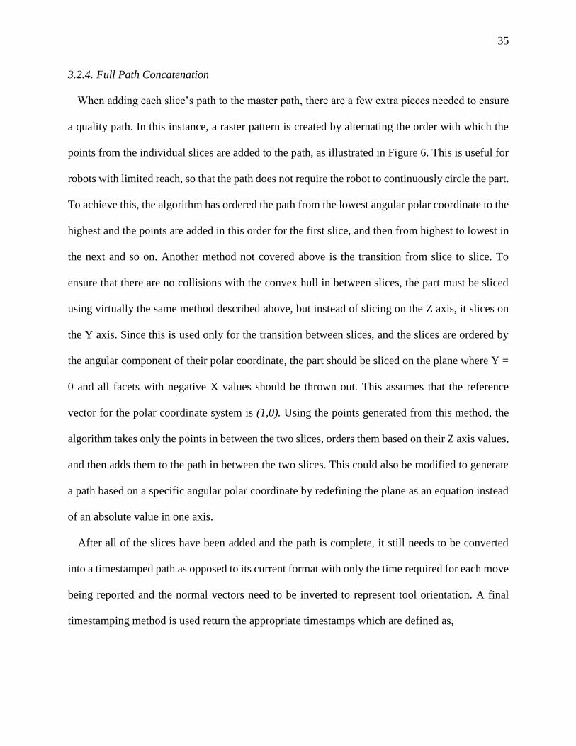
3.2.4. Full Path Concatenation

When adding each slice’s path to the master path, there are a few extra pieces needed to ensure

a quality path. In this instance, a raster pattern is created by alternating the order with which the

points from the individual slices are added to the path, as illustrated in Figure 6. This is useful for

robots with limited reach, so that the path does not require the robot to continuously circle the part.

To achieve this, the algorithm has ordered the path from the lowest angular polar coordinate to the

highest and the points are added in this order for the first slice, and then from highest to lowest in

the next and so on. Another method not covered above is the transition from slice to slice. To

ensure that there are no collisions with the convex hull in between slices, the part must be sliced

using virtually the same method described above, but instead of slicing on the Z axis, it slices on

the Y axis. Since this is used only for the transition between slices, and the slices are ordered by

the angular component of their polar coordinate, the part should be sliced on the plane where Y =

0 and all facets with negative X values should be thrown out. This assumes that the reference

vector for the polar coordinate system is (1,0). Using the points generated from this method, the

algorithm takes only the points in between the two slices, orders them based on their Z axis values,

and then adds them to the path in between the two slices. This could also be modified to generate

a path based on a specific angular polar coordinate by redefining the plane as an equation instead

of an absolute value in one axis.

After all of the slices have been added and the path is complete, it still needs to be converted

into a timestamped path as opposed to its current format with only the time required for each move

being reported and the normal vectors need to be inverted to represent tool orientation. A final

timestamping method is used return the appropriate timestamps which are defined as,

36

𝐺𝑚𝑎𝑠𝑡𝑒𝑟 = {[𝒑𝑔, 𝒓𝑔, 𝑡𝑔] |{𝑔 = 0 , 𝑡𝑔 = 0

𝑒𝑙𝑠𝑒 , 𝑡𝑔 = 𝑡𝑔−1 + ∆𝑡𝑔−1} ∀ 𝒈 ∈ 𝐺𝑚𝑎𝑠𝑡𝑒𝑟}

(23)

where 𝑡𝑔 is the timestamp of pair g, ∆𝑡𝑔−1 is the time needed to move from 𝒑𝑔−1 to point 𝒑𝑔,

𝐺𝑚𝑎𝑠𝑡𝑒𝑟 is the ordered set of all observations in the entire trajectory, and 𝒓𝑔 is the toolpath

orientation vector for observation g, which is defined as,

𝒓𝑔 = −�̂�𝑔 (24)

where �̂�𝑔 is the corresponding normal vector of observation g identified earlier. This is where the

algorithm turns a list of points into a time-based trajectory for a robot to realistically follow. The

finished path is then passed on to a either the user for review or the robot itself for execution.

Figure 8: Raster Path Concatenation

3.2.5. Partial Path Creation

In some instances, a full path plan may not be necessary. A user could have pre-existing

knowledge of the parts condition and only need to plan for a specific area, or the user could

observe some flaws in the original path plans simulation and opt to add an additional partial path

to address the issue. Partial path planning can also be utilized to prevent robotic accessibility

issues, such as singularities, collisions, and reach issues. Previous research lays out a framework

37

and infrastructure for facilitating these decisions by allowing the user to select individual facets

on the part for partial path planning [38]. In these scenarios, this path planner uses the extreme

values of the selected facets Z values and angular components of the centroids polar coordinate

to select the necessary parts of the path. Aside from the selection process, the algorithm proceeds

as normal. The slices selected as part of the partial path are defined as,

𝑆𝑝𝑎𝑟𝑡 = {𝑠 | 𝑍𝑐min≤ 𝑠𝑍 ≤ 𝑍𝑐max

∧ 𝑠 ∈ 𝑆} (25)

where 𝑍𝑐𝑚𝑖𝑛 and 𝑍𝑐𝑚𝑎𝑥

are the minimum and maximum Z values of the selected facets and 𝑠𝑍 is

the Z value of slice s. Within each selected slice, the planner defines the path points to be

selected as,

𝑃𝑠 = {𝒑 | 𝜑min ≤ 𝜑𝒑 ≤ 𝜑max ∧ 𝒑 ∈ 𝑃𝑠} (26)

where 𝜑𝒑 is the angular polar coordinate of the path point 𝒑, and 𝜑min and 𝜑max are the extreme

angular polar coordinates of all of the selected facets. The user is then given the opportunity to

again observe the resulting path and make any additions if necessary.

While this method is relatively easy to implement, it is computationally inefficient. An

alternative method would be to define a partial convex hull of only the selected facets and then

run the algorithm as usual with the partial hull. If a partial convex hull is implemented, there

needs to be some methods developed to ensure that the resulting path does not violate the convex

hull of the entire part, otherwise a collision is very likely for non-continuous selections and even

a possibility for continuous selections. Specifically, since a convex hull is built without regards

to the orientation of the original facets inside the convex hull, so the resulting toolpath would

still wrap completely around the new convex hull even if the selected facets were only on one

38

side. The only way to then avoid the method utilized in this planner, would be to successfully

link facets on the convex hull to facets on the original point and build a partial convex hull from

only the corresponding facets.

3.2.6. Adaptive Methods

To this point, all path planning has been done on the convex hull. This will henceforth be referred

to as the “naïve” tool trajectory since it does not consider the underlying surface topology. The

following sections describe methods for adapting the naïve trajectory based on the actual part

surface. This is accomplished by associating features of the underlying surface with segments of

the toolpath and adjusting the tool offset distance and/or velocity based on aggregate descriptions

of the underlying surface’s position and orientation with respect to the convex hull.

The true surface is represented by a set of ordered pairs of points and normal vectors, 𝐶 = {𝒄, �̂�}.

The points are sampled from the workpiece’s tessellated mesh, and each point is paired with the

unit normal vector of the facet from which it was sampled. To avoid ambiguity regarding the unit

To this point, all path planning has been done on the convex hull. This will henceforth be referred

to as the “naïve” tool trajectory since it does not consider the underlying surface topology. The

following sections describe methods for adapting the naïve trajectory based on the actual part

surface. This is accomplished by associating features of the underlying surface with segments of

the toolpath and adjusting the tool offset distance and/or velocity based on aggregate descriptions

of the underlying surface’s position and orientation with respect to the convex hull.

The true surface is represented by a set of ordered pairs of points and normal vectors, 𝐶 = {𝒄, �̂�}.

The points are sampled from the workpiece’s tessellated mesh, and each point is paired with the

unit normal vector of the facet from which it was sampled. To avoid ambiguity regarding the unit

normal, points should not be sampled from facet edges.

39

Sampling strategy is a tradeoff between resolution and computational load, and it has

implications for how each surface facet influences the adjusted tool trajectory. A simple method

is to take the centroid of each facet. This insures that each facet is represented in the ensuing

calculations but has disadvantages when facet size varies significantly or facet aspect ratios are

high: Areas of high curvature (many small facets) can dominate areas of low curvature (fewer,

larger facets), and the centroids of high-aspect-ratio facets can be far from their associated vertices.

The disadvantages may be mitigated by enforcing a uniform sampling resolution within facets;

however, this can significantly increase the number of points and thus the computational load. A

third option is to densely sample the mesh and then down sample via a voxel grid filter (VGF)

[39]. The VGF overlays a three-dimensional grid onto the point cloud; all points within each voxel

are represented their centroid and normal vectors are represented by their average. The resolution

versus computation tradeoff is managed by setting the grid size, though the VGF itself consumes

computational resources. For simplicity, and without loss of generality, this research uses the first

method – representing each facet via its centroid.

Associating elements of C with segments of the slice polygon on the convex hull is done slice-

wise. Let

𝐶𝑠 = {𝒄, �̂� | 𝑍𝑠min≤ 𝑐𝑍 ≤ 𝑍𝑠max

} ∀ 𝑐 ∈ 𝐶 (27)

be the elements of C associated with slice s, where 𝑐𝑍 is the Z coordinate of point c and 𝑍𝑠min and

𝑍𝑠max are defined as,

𝑍𝑠min= ℎ𝑠 −

𝑤𝐴

2 𝑍𝑠max

= ℎ𝑠 + 𝑤𝐴

2 (28)

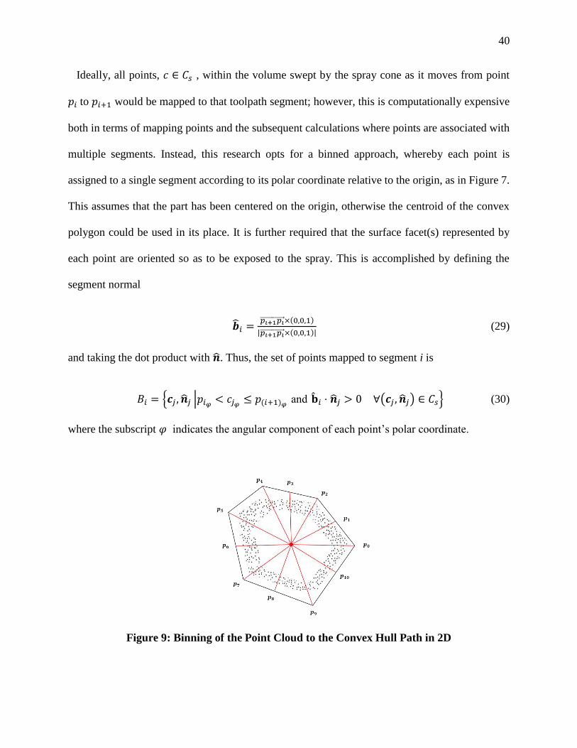
40

Ideally, all points, 𝑐 ∈ 𝐶𝑠 , within the volume swept by the spray cone as it moves from point

𝑝𝑖 to 𝑝𝑖+1 would be mapped to that toolpath segment; however, this is computationally expensive

both in terms of mapping points and the subsequent calculations where points are associated with

multiple segments. Instead, this research opts for a binned approach, whereby each point is

assigned to a single segment according to its polar coordinate relative to the origin, as in Figure 7.

This assumes that the part has been centered on the origin, otherwise the centroid of the convex

polygon could be used in its place. It is further required that the surface facet(s) represented by

each point are oriented so as to be exposed to the spray. This is accomplished by defining the

segment normal

�̂�𝑖 =𝑝𝑖+1𝑝𝑖⃗⃗ ⃗⃗ ⃗⃗ ⃗⃗ ⃗⃗ ⃗⃗ ⃗⃗ ×(0,0,1)

|𝑝𝑖+1𝑝𝑖⃗⃗ ⃗⃗ ⃗⃗ ⃗⃗ ⃗⃗ ⃗⃗ ⃗⃗ ×(0,0,1)| (29)

and taking the dot product with �̂�. Thus, the set of points mapped to segment i is

𝐵𝑖 = {𝒄𝑗 , �̂�𝑗 |𝑝𝑖𝜑 < 𝑐𝑗𝜑 ≤ 𝑝(𝑖+1)𝜑 and �̂�𝑖 ⋅ �̂�𝑗 > 0 ∀(𝒄𝑗 , �̂�𝑗) ∈ 𝐶𝑠} (30)

where the subscript 𝜑 indicates the angular component of each point’s polar coordinate.

Figure 9: Binning of the Point Cloud to the Convex Hull Path in 2D

41

Using this collection of binned points, the algorithm has the option to adapt the path by

adjusting the distance from the part, the velocity of the move or both for each bin within each

slice. The process for using both adaptive methods is relatively straight forward when used

separately, the distance-based method looks at the aggregate distance from the end effector to all

of the affected points and adjusts accordingly and the time-based method looks at the aggregate

incidence angle between the orientation of the end effector and the normal vector of each

affected point. However, there is one constraint on how they can be used together. Due to the

change in positions created by the distance-based adapting method, which can have an effect on

the distance between points and thus the time needed to complete the move, the time-based

adapting method must be used after the distance-based method for accurate results.

One of the shortcomings of this methodology is the fact that each adaptive algorithm only

considers one data type when making a decision on how to adapt the path. Ideally, every decision

should be made with all of the available data, but sometimes different data types can skew the

results. In this case, using the incidence angle as an indicator of how much the path offset distance

should be adjusted would cause the distance to be adapted too much to the point where the sprayer

width is narrower than the offset width. This causes gaps in the raster pattern which then requires

replanning later on. Alternatively, using distance from the part to influence the velocity of the end

effector does not cause the same path breaking issues, but it doesn’t necessarily help all that much

either. If the end effector is already too far away, the overall performance of the path would be

much better served by adjusting the distance rather than extending the exposure time and thus

lengthening the overall execution time.

42

3.2.6.1.Distance Based Adapting

Given the bins of the path being adapted and the point cloud points that have been matched to

each bin, the algorithm defines the distance from each point to the line created by the two end

points of the matched bin [40]. Using this distance, the adaptive process can begin by defining the

adjustment value for each bin as,

𝜓𝑏 = min(𝑑𝐴𝐺𝑏− 𝑑O , 𝑥𝑑O) ∀ 𝑏 ∈ 𝐵𝑠 (31)

where 𝐵𝑠 is the set of all bins on slice s, x represents the maximum percentage that the path can

adapt by with regards to 𝑑O, and 𝑑𝐴𝐺𝑏 is defined as the aggregate distance value of all points in the

bin, which can vary based on the aggregation method. Ideally, this returns a value of zero, meaning

no adjustment is needed and the aggregate distance is equal to the desired offset distance. The

adjustment value is limited in range so that the path will not be moved within the convex hull by

over adjusting. In this case, x = 0.95. This is necessary because a value greater than or equal to 1

would result in an adjustment greater than the offset distance itself which would cause the new

position to be inside or on the convex hull. While this may not create any collision issues, there is

always the possibility and thus is must be accounted for. Alternatively, a minimum distance could

be defined and the adjustment would occur on the remaining distance beyond the minimum

distance. It should also be noted that the aggregate method used depends on the user’s initial input.

If necessary, the new path points are determined by,

𝒑 = 𝒑 − (𝒏�̂� 𝜓𝑝 ) ∀ 𝒑 ∈ 𝑃𝑠 (32)

where 𝒏�̂� is the unit vector of the corresponding surface normal, 𝑃𝑠 is the path for slice s, and 𝜓𝑝

is the adjustment value of the path point which is defined as,

43

𝜓𝑝 = max (𝜓𝑏𝑝 , 𝜓𝑏𝑝−1

) (33)

where 𝜓𝑏𝑝 is the adjustment value of point p in bin b. The max of the two bins that share the point

is used to ensure that the bin needing the most adjustment gets it. For path smoothness, a moving

average of the adjacent bins can be used to determine how much adjustment is needed for each bin

by taking the mean of a few adjacent values on both sides of the bin. An example of distance-based

adaptation is shown below in Figure 8 as an individual slice of Part C, where both the naïve path,

in blue, and the distance adapted path, in orange, have been plotted along with the facets that are

captured within the slice, the exact slicing height is shown to the right of the path analysis.

Figure 10: Distance vs Naive Path Plan

3.2.6.2.Time Based Adapting

For this adaptive method, the algorithm determines an incidence value for each point within each

bin as illustrated in Figure 9. The incidence value is defined as,

𝜃𝑏𝑐 = (𝒏𝒃𝟏 + 𝒏𝒃𝟐) ∙ 𝒏𝒄 ∀ 𝑏 ∈ 𝐵𝑠

∀ 𝑐 ∈ 𝑏 (34)

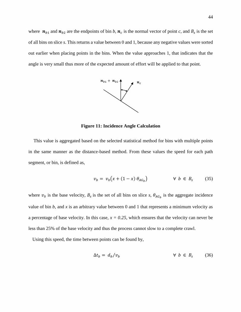
44

where 𝒏𝑏1 and 𝒏𝑏2 are the endpoints of bin b, 𝒏𝑐 is the normal vector of point c, and 𝐵𝑠 is the set

of all bins on slice s. This returns a value between 0 and 1, because any negative values were sorted

out earlier when placing points in the bins. When the value approaches 1, that indicates that the

angle is very small thus more of the expected amount of effort will be applied to that point.

Figure 11: Incidence Angle Calculation

This value is aggregated based on the selected statistical method for bins with multiple points

in the same manner as the distance-based method. From these values the speed for each path

segment, or bin, is defined as,

𝑣𝑏 = 𝑣0(𝑥 + (1 − 𝑥) 𝜃𝐴𝐺𝑏) ∀ 𝑏 ∈ 𝐵𝑠 (35)

where 𝑣0 is the base velocity, 𝐵𝑠 is the set of all bins on slice s, 𝜃𝐴𝐺𝑏 is the aggregate incidence

value of bin b, and x is an arbitrary value between 0 and 1 that represents a minimum velocity as

a percentage of base velocity. In this case, x = 0.25, which ensures that the velocity can never be

less than 25% of the base velocity and thus the process cannot slow to a complete crawl.

Using this speed, the time between points can be found by,

∆𝑡𝑏 = 𝑑𝑏 𝑣𝑏⁄ ∀ 𝑏 ∈ 𝐵𝑠 (36)

45

where ∆𝑡𝑏 is the time between the endpoints of bin b, 𝑑𝑏 is the distance between the endpoints of

bin b, and 𝐵𝑠 is the set of all bins on slice s. These new time values replace the previously defined

values from the original path.

In order to account for the change in speed, an adjusted adaptive value is derived to represent

the current amount of work being done during the entire move from one end of the bin to the other.

This value is defined as,

𝜏𝑏𝑐 = 𝜃𝑏𝑐 + (1 − 𝑣𝑏

𝑣0)

∀ 𝑐 ∈ 𝐶∀ 𝑏 ∋ 𝑐

(37)

where 𝜃𝑏𝑐 is the incidence angle between point c and the end effector moving through bin b, which

is defined for each bin a point falls in. This results in values that approach 1, the ideal value, but

do not achieve 1, unless it was there before and required no adaptation. The closeness to 1 for a

given point can be manipulated by changing the value of x when determining 𝑣𝑏, where the smaller

the value, the closer to 1 these values can become at the expense of time.

3.2.7. Analysis

In order to properly analyze the quality of the path, a single impingement value was assigned to

each point in the point cloud derived from the original part that combined measures of both

adaptive methods. This impingement value is defined as,

𝛾𝑐 = ∑ (1

𝑑𝑏𝑐2 𝜏𝑏𝑐) ∀ 𝑏 ∋ 𝑐 ∀ 𝑐 ∈ 𝐶 (38)

where 𝜏𝑏𝑐 is the adjusted time-based value for point c with regards to bin b, 𝑑𝑏𝑐 is the distance

from point c to the path of the end effector in bin b and 1

𝑑𝑏𝑐2 is derived from the well-known Inverse

46

Square Law. The summation across all bins b that contain point c accounts for any overlap between

slices that may cause a point to be captured twice and thus receive more work overall.

3.2.8. Experimental Design

In order to determine the best method for producing better toolpaths, two factors were

considered. The type of adaptive algorithm used, which has two levels: Distance and Distance +

Time, and the type of statistical aggregate method used, which has four levels: Mean, Mode, Min

and Max. These factors, along with a Naïve path, with no adaptive adjustments, combine to create

nine different treatments. Aside from the usual summary statistics, a bin metric was developed to

better measure the distribution of total cleaning applied across the entire part and is defined as,

𝜁 = ∑ ∑ {𝑏min ≤ 𝛾𝑐 < 𝑏max , 𝑗 𝑒𝑙𝑠𝑒 , 0

} 𝛽𝑗=1

𝜂𝑐=0 𝜂⁄ (39)

where η is the number of facets on the part, 𝛾𝑐 is the impingement value of facet c, 𝛽 is the number

of bins, j is the bin iterator, and 𝑏min and 𝑏max are the endpoints of each bin that are defined as,

𝑏min = 𝛾min + (𝑗 − 1)𝛾max − 𝛾min

𝛽 𝑏max = 𝛾min + 𝑗

𝛾max − 𝛾min

𝛽 (40)

where 𝛾min is the minimum impingement value and 𝛾max is the maximum impingement value of

all parts being compared. This yields a result between one and the number of bins, with higher

values indicating a better overall toolpath. The total time and distance needed to complete the

toolpath were also considered to see what kind of trade-off occurs when the path is adapted.

A set of five test parts were chosen to be used in this analysis as shown in Figure 10. Two of the

parts, A and B, were specifically designed to demonstrate how the planner makes adjustments to

the path, while the other three were taken from online 3D CAD databases to represent common

geometries encountered in the real world. Each of the parts were sliced using the exact same

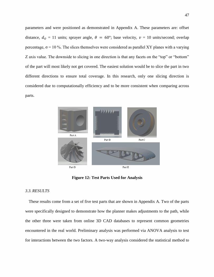
47

parameters and were positioned as demonstrated in Appendix A. These parameters are: offset

distance, 𝑑𝑂 = 11 units; sprayer angle, 𝜃 = 60°; base velocity, 𝑣 = 10 units/second; overlap

percentage, σ = 10 %. The slices themselves were considered as parallel XY planes with a varying

Z axis value. The downside to slicing in one direction is that any facets on the “top” or “bottom”

of the part will most likely not get covered. The easiest solution would be to slice the part in two

different directions to ensure total coverage. In this research, only one slicing direction is

considered due to computationally efficiency and to be more consistent when comparing across

parts.

Figure 12: Test Parts Used for Analysis

3.3. RESULTS

These results come from a set of five test parts that are shown in Appendix A. Two of the parts

were specifically designed to demonstrate how the planner makes adjustments to the path, while

the other three were taken from online 3D CAD databases to represent common geometries

encountered in the real world. Preliminary analysis was performed via ANOVA analysis to test

for interactions between the two factors. A two-way analysis considered the statistical method to

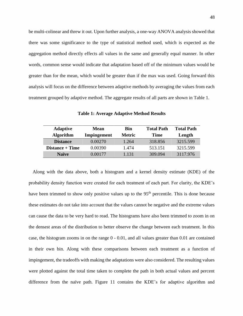
48

be multi-colinear and threw it out. Upon further analysis, a one-way ANOVA analysis showed that

there was some significance to the type of statistical method used, which is expected as the

aggregation method directly effects all values in the same and generally equal manner. In other

words, common sense would indicate that adaptation based off of the minimum values would be

greater than for the mean, which would be greater than if the max was used. Going forward this

analysis will focus on the difference between adaptive methods by averaging the values from each

treatment grouped by adaptive method. The aggregate results of all parts are shown in Table 1.

Table 1: Average Adaptive Method Results

Adaptive

Algorithm

Mean

Impingement

Bin

Metric

Total Path

Time

Total Path

Length

Distance 0.00270 1.264 318.856 3215.599

Distance + Time 0.00390 1.474 513.151 3215.599

Naïve 0.00177 1.131 309.094 3117.976

Along with the data above, both a histogram and a kernel density estimate (KDE) of the

probability density function were created for each treatment of each part. For clarity, the KDE’s

have been trimmed to show only positive values up to the 95th percentile. This is done because

these estimates do not take into account that the values cannot be negative and the extreme values

can cause the data to be very hard to read. The histograms have also been trimmed to zoom in on

the densest areas of the distribution to better observe the change between each treatment. In this

case, the histogram zooms in on the range 0 - 0.01, and all values greater than 0.01 are contained

in their own bin. Along with these comparisons between each treatment as a function of

impingement, the tradeoffs with making the adaptations were also considered. The resulting values

were plotted against the total time taken to complete the path in both actual values and percent

difference from the naïve path. Figure 11 contains the KDE’s for adaptive algorithm and

49

aggregation method as well as a plot of each treatments bin metric vs time in columns 1-3

respectively, and each row A-E references the corresponding part. Individual part results and heat

maps are also included in the text below. In the heatmaps, red indicates more cleaning and blue

indicates less or none at all. All other figures and results are contained in the appendices. Appendix

A contains the original parts, Appendix B contains the KDE’s, Appendix C contains the

histograms, Appendix D contains the trade-off plots, Appendix E contains the individual treatment

results for each part, and Appendix F contains a nomenclature table for all equations.

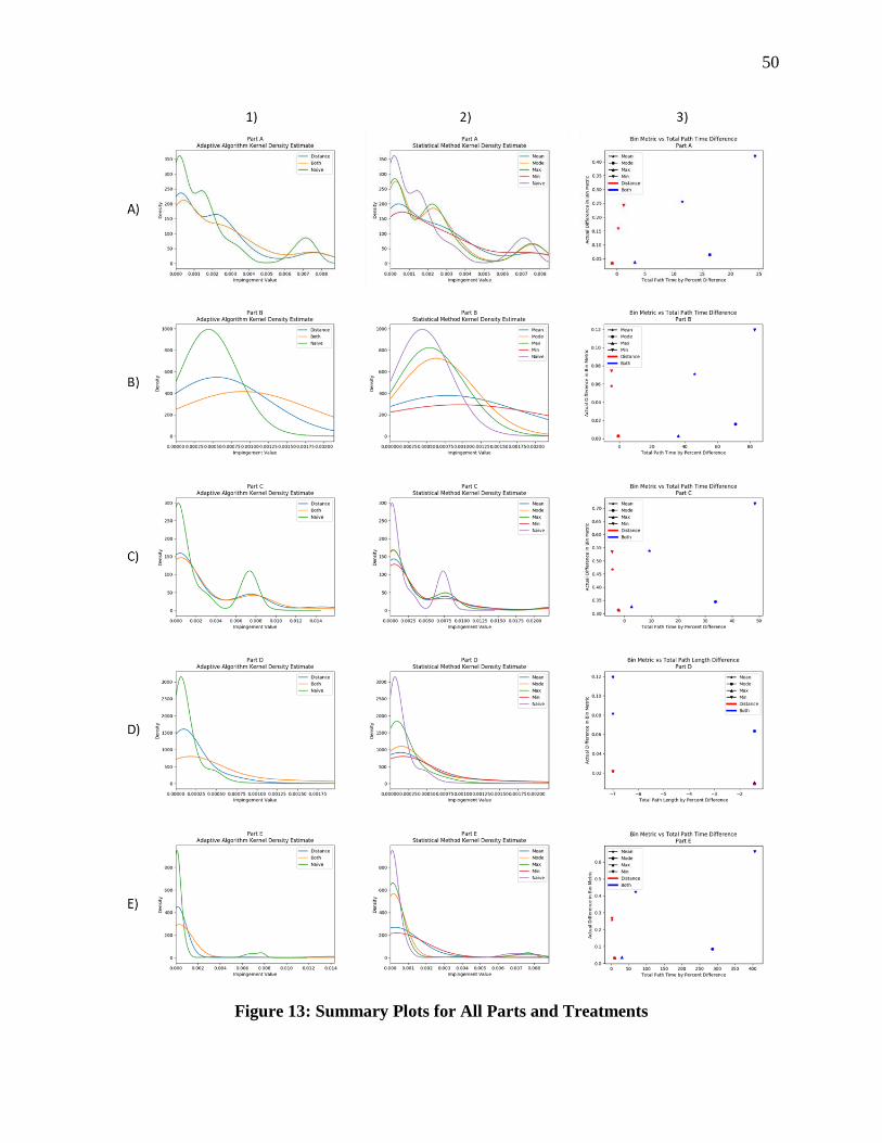
50

Figure 13: Summary Plots for All Parts and Treatments

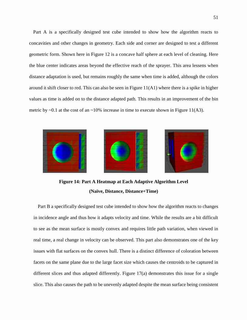
51

Part A is a specifically designed test cube intended to show how the algorithm reacts to

concavities and other changes in geometry. Each side and corner are designed to test a different

geometric form. Shown here in Figure 12 is a concave half sphere at each level of cleaning. Here

the blue center indicates areas beyond the effective reach of the sprayer. This area lessens when

distance adaptation is used, but remains roughly the same when time is added, although the colors

around it shift closer to red. This can also be seen in Figure 11(A1) where there is a spike in higher

values as time is added on to the distance adapted path. This results in an improvement of the bin

metric by ~0.1 at the cost of an ~10% increase in time to execute shown in Figure 11(A3).

Figure 14: Part A Heatmap at Each Adaptive Algorithm Level

(Naïve, Distance, Distance+Time)

Part B a specifically designed test cube intended to show how the algorithm reacts to changes

in incidence angle and thus how it adapts velocity and time. While the results are a bit difficult

to see as the mean surface is mostly convex and requires little path variation, when viewed in

real time, a real change in velocity can be observed. This part also demonstrates one of the key

issues with flat surfaces on the convex hull. There is a distinct difference of coloration between

facets on the same plane due to the large facet size which causes the centroids to be captured in

different slices and thus adapted differently. Figure 17(a) demonstrates this issue for a single

slice. This also causes the path to be unevenly adapted despite the mean surface being consistent

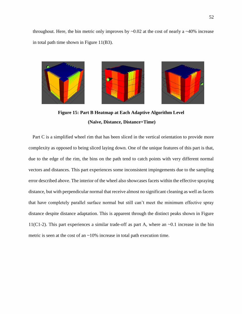
52

throughout. Here, the bin metric only improves by ~0.02 at the cost of nearly a ~40% increase

in total path time shown in Figure 11(B3).

Figure 15: Part B Heatmap at Each Adaptive Algorithm Level

(Naïve, Distance, Distance+Time)

Part C is a simplified wheel rim that has been sliced in the vertical orientation to provide more

complexity as opposed to being sliced laying down. One of the unique features of this part is that,

due to the edge of the rim, the bins on the path tend to catch points with very different normal

vectors and distances. This part experiences some inconsistent impingements due to the sampling

error described above. The interior of the wheel also showcases facets within the effective spraying

distance, but with perpendicular normal that receive almost no significant cleaning as well as facets

that have completely parallel surface normal but still can’t meet the minimum effective spray

distance despite distance adaptation. This is apparent through the distinct peaks shown in Figure

11(C1-2). This part experiences a similar trade-off as part A, where an ~0.1 increase in the bin

metric is seen at the cost of an ~10% increase in total path execution time.

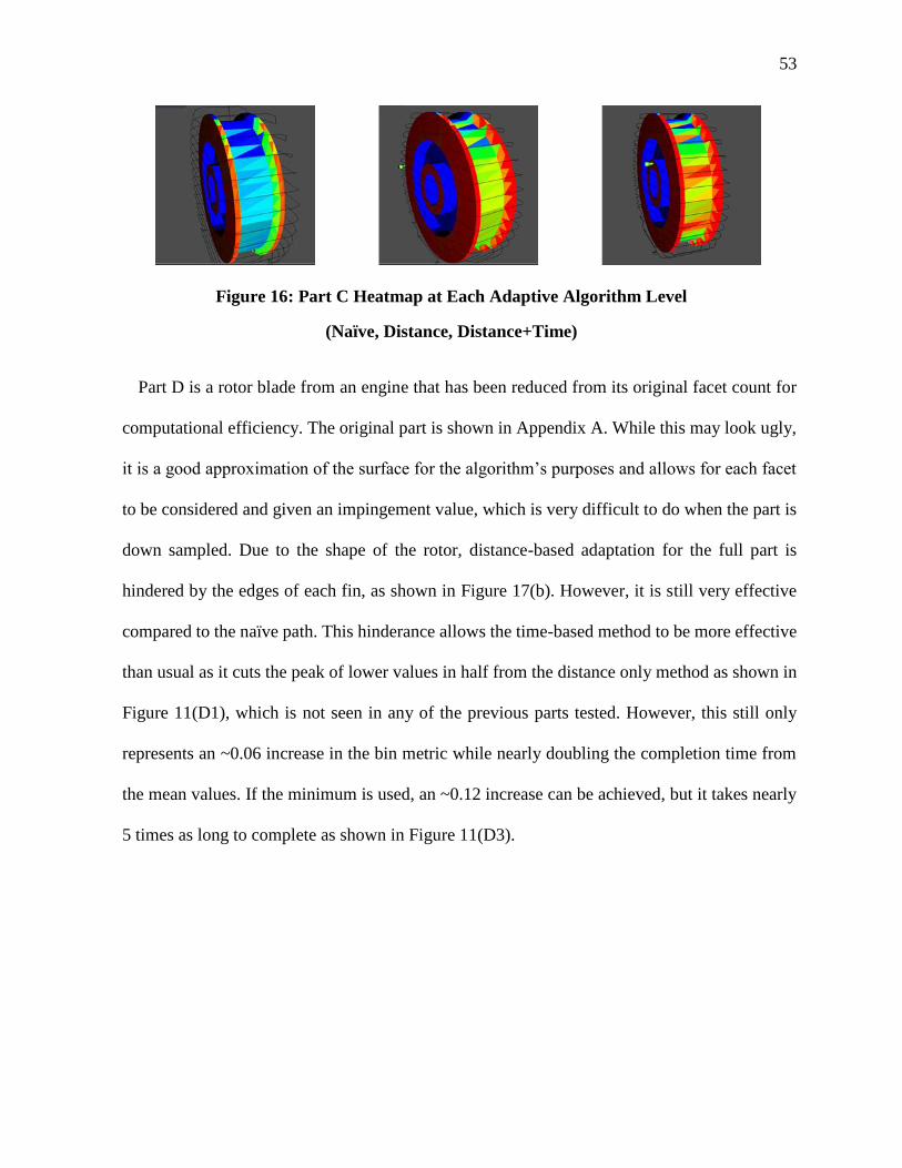
53

Figure 16: Part C Heatmap at Each Adaptive Algorithm Level

(Naïve, Distance, Distance+Time)

Part D is a rotor blade from an engine that has been reduced from its original facet count for

computational efficiency. The original part is shown in Appendix A. While this may look ugly,

it is a good approximation of the surface for the algorithm’s purposes and allows for each facet

to be considered and given an impingement value, which is very difficult to do when the part is

down sampled. Due to the shape of the rotor, distance-based adaptation for the full part is

hindered by the edges of each fin, as shown in Figure 17(b). However, it is still very effective

compared to the naïve path. This hinderance allows the time-based method to be more effective

than usual as it cuts the peak of lower values in half from the distance only method as shown in

Figure 11(D1), which is not seen in any of the previous parts tested. However, this still only

represents an ~0.06 increase in the bin metric while nearly doubling the completion time from

the mean values. If the minimum is used, an ~0.12 increase can be achieved, but it takes nearly

5 times as long to complete as shown in Figure 11(D3).

54

Figure 17: Part D Heatmap at Each Adaptive Algorithm Level

(Naïve, Distance, Distance+Time)

Part E is a cross section of an airplane wing that has also been reduced to facilitate computational

speed. Here the reduction does not have a large effect on the visible geometry. This part represents

an extreme challenge of tool point accessibility. In this case, the sprayer cannot invade the convex

hull, which makes it very hard to effectively cover a large portion of the part. This can be seen in

the relatively small change in the distribution in Figure 11(E1) as well as in the individual slice

path in Figure 17(c). Here, the naïve path’s peak at higher impingement values is smoothed out

across the higher values and appears to disappear while the lower values are slightly reduced and

shifted only by a very little bit. This is a part, that while easily planned for externally, the interior

will continue to remain a challenge until effective accessibility algorithms are included in the path

planning. This difficulty in accessing the interior is seen most sharply in the difference between

the distance and distance + time bin metrics. Here there is an increase of ~0.15, the highest of all

the tested parts, at a cost of only a ~50% increase in execution time., which is much better than the

~500% needed to achieve a worse result in part D.

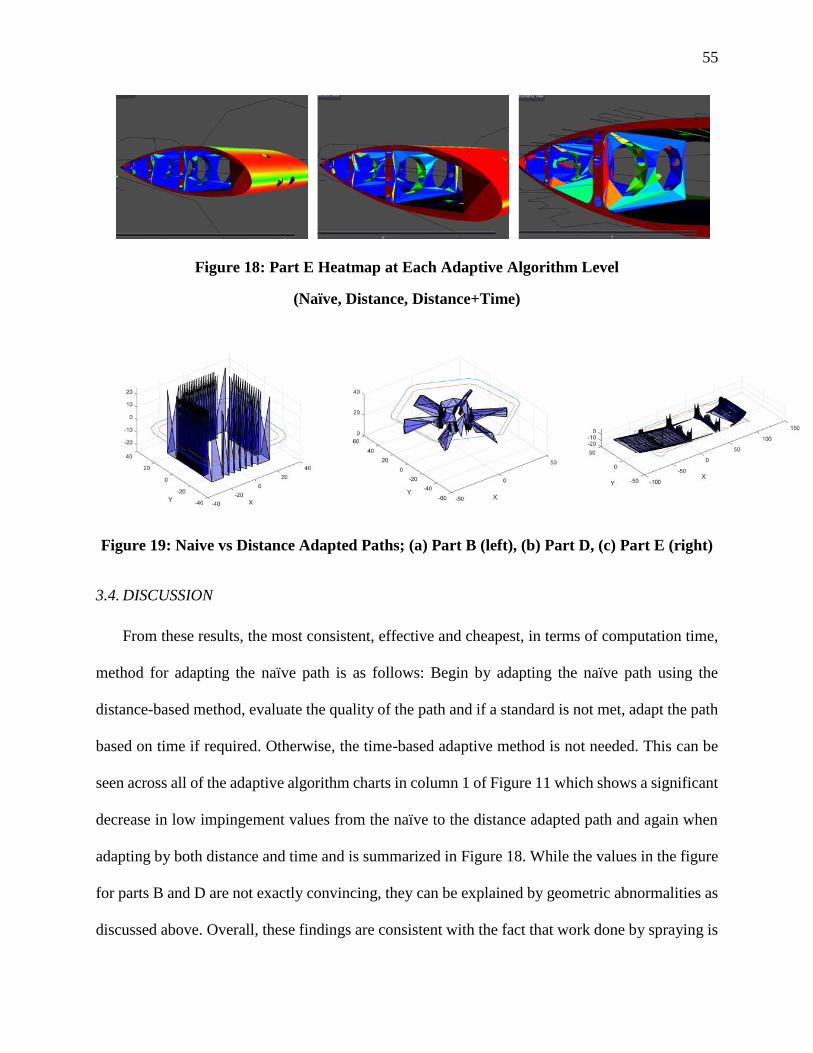
55

Figure 18: Part E Heatmap at Each Adaptive Algorithm Level

(Naïve, Distance, Distance+Time)

Figure 19: Naive vs Distance Adapted Paths; (a) Part B (left), (b) Part D, (c) Part E (right)

3.4. DISCUSSION

From these results, the most consistent, effective and cheapest, in terms of computation time,

method for adapting the naïve path is as follows: Begin by adapting the naïve path using the

distance-based method, evaluate the quality of the path and if a standard is not met, adapt the path

based on time if required. Otherwise, the time-based adaptive method is not needed. This can be

seen across all of the adaptive algorithm charts in column 1 of Figure 11 which shows a significant

decrease in low impingement values from the naïve to the distance adapted path and again when

adapting by both distance and time and is summarized in Figure 18. While the values in the figure

for parts B and D are not exactly convincing, they can be explained by geometric abnormalities as

discussed above. Overall, these findings are consistent with the fact that work done by spraying is

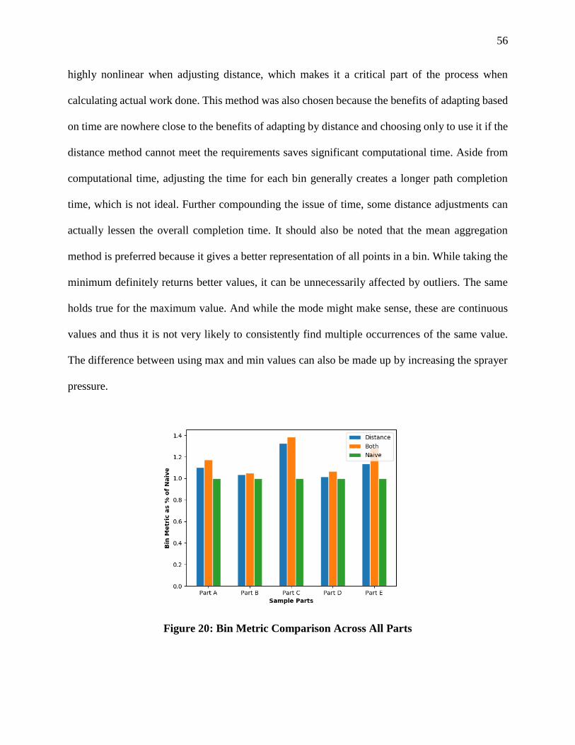
56

highly nonlinear when adjusting distance, which makes it a critical part of the process when

calculating actual work done. This method was also chosen because the benefits of adapting based

on time are nowhere close to the benefits of adapting by distance and choosing only to use it if the

distance method cannot meet the requirements saves significant computational time. Aside from

computational time, adjusting the time for each bin generally creates a longer path completion

time, which is not ideal. Further compounding the issue of time, some distance adjustments can

actually lessen the overall completion time. It should also be noted that the mean aggregation

method is preferred because it gives a better representation of all points in a bin. While taking the

minimum definitely returns better values, it can be unnecessarily affected by outliers. The same

holds true for the maximum value. And while the mode might make sense, these are continuous

values and thus it is not very likely to consistently find multiple occurrences of the same value.

The difference between using max and min values can also be made up by increasing the sprayer

pressure.

Figure 20: Bin Metric Comparison Across All Parts

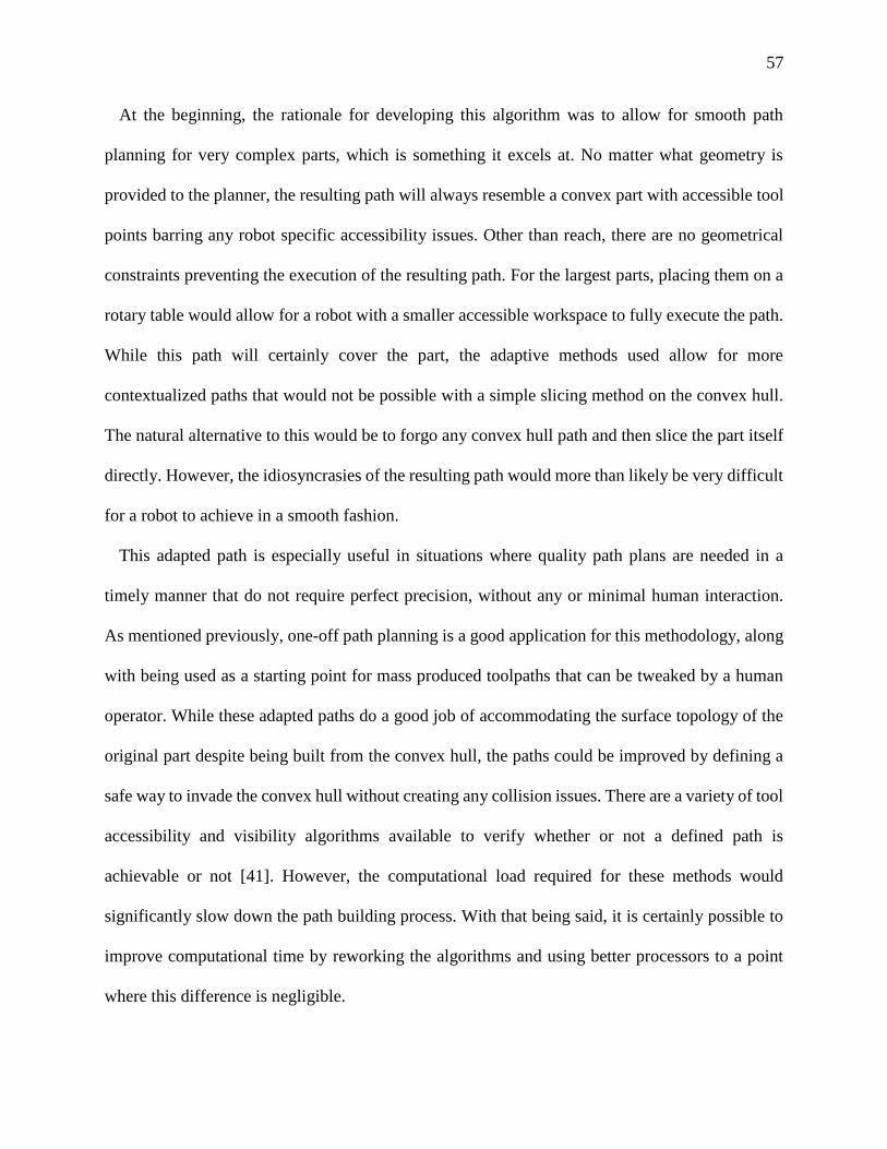
57

At the beginning, the rationale for developing this algorithm was to allow for smooth path

planning for very complex parts, which is something it excels at. No matter what geometry is

provided to the planner, the resulting path will always resemble a convex part with accessible tool

points barring any robot specific accessibility issues. Other than reach, there are no geometrical

constraints preventing the execution of the resulting path. For the largest parts, placing them on a

rotary table would allow for a robot with a smaller accessible workspace to fully execute the path.

While this path will certainly cover the part, the adaptive methods used allow for more

contextualized paths that would not be possible with a simple slicing method on the convex hull.

The natural alternative to this would be to forgo any convex hull path and then slice the part itself

directly. However, the idiosyncrasies of the resulting path would more than likely be very difficult

for a robot to achieve in a smooth fashion.

This adapted path is especially useful in situations where quality path plans are needed in a

timely manner that do not require perfect precision, without any or minimal human interaction.

As mentioned previously, one-off path planning is a good application for this methodology, along

with being used as a starting point for mass produced toolpaths that can be tweaked by a human

operator. While these adapted paths do a good job of accommodating the surface topology of the

original part despite being built from the convex hull, the paths could be improved by defining a

safe way to invade the convex hull without creating any collision issues. There are a variety of tool

accessibility and visibility algorithms available to verify whether or not a defined path is

achievable or not [41]. However, the computational load required for these methods would

significantly slow down the path building process. With that being said, it is certainly possible to

improve computational time by reworking the algorithms and using better processors to a point

where this difference is negligible.

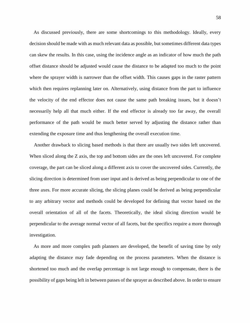
58

As discussed previously, there are some shortcomings to this methodology. Ideally, every

decision should be made with as much relevant data as possible, but sometimes different data types

can skew the results. In this case, using the incidence angle as an indicator of how much the path

offset distance should be adjusted would cause the distance to be adapted too much to the point

where the sprayer width is narrower than the offset width. This causes gaps in the raster pattern

which then requires replanning later on. Alternatively, using distance from the part to influence

the velocity of the end effector does not cause the same path breaking issues, but it doesn’t

necessarily help all that much either. If the end effector is already too far away, the overall

performance of the path would be much better served by adjusting the distance rather than

extending the exposure time and thus lengthening the overall execution time.

Another drawback to slicing based methods is that there are usually two sides left uncovered.

When sliced along the Z axis, the top and bottom sides are the ones left uncovered. For complete

coverage, the part can be sliced along a different axis to cover the uncovered sides. Currently, the

slicing direction is determined from user input and is derived as being perpendicular to one of the

three axes. For more accurate slicing, the slicing planes could be derived as being perpendicular

to any arbitrary vector and methods could be developed for defining that vector based on the

overall orientation of all of the facets. Theoretically, the ideal slicing direction would be

perpendicular to the average normal vector of all facets, but the specifics require a more thorough

investigation.

As more and more complex path planners are developed, the benefit of saving time by only

adapting the distance may fade depending on the process parameters. When the distance is

shortened too much and the overlap percentage is not large enough to compensate, there is the

possibility of gaps being left in between passes of the sprayer as described above. In order to ensure

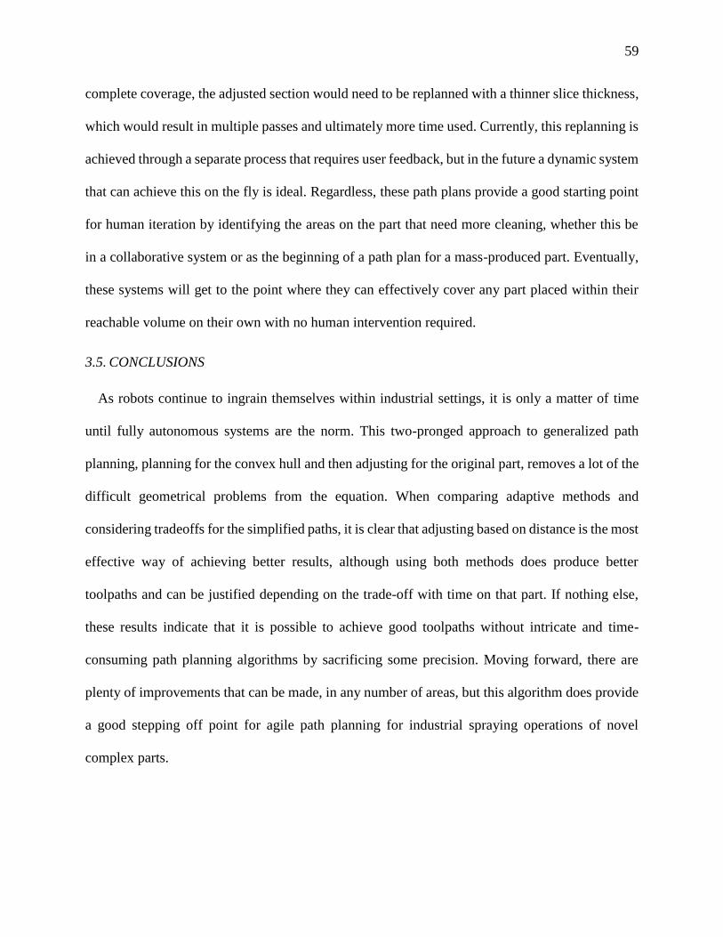
59

complete coverage, the adjusted section would need to be replanned with a thinner slice thickness,

which would result in multiple passes and ultimately more time used. Currently, this replanning is

achieved through a separate process that requires user feedback, but in the future a dynamic system

that can achieve this on the fly is ideal. Regardless, these path plans provide a good starting point

for human iteration by identifying the areas on the part that need more cleaning, whether this be

in a collaborative system or as the beginning of a path plan for a mass-produced part. Eventually,

these systems will get to the point where they can effectively cover any part placed within their

reachable volume on their own with no human intervention required.

3.5. CONCLUSIONS

As robots continue to ingrain themselves within industrial settings, it is only a matter of time

until fully autonomous systems are the norm. This two-pronged approach to generalized path

planning, planning for the convex hull and then adjusting for the original part, removes a lot of the

difficult geometrical problems from the equation. When comparing adaptive methods and

considering tradeoffs for the simplified paths, it is clear that adjusting based on distance is the most

effective way of achieving better results, although using both methods does produce better

toolpaths and can be justified depending on the trade-off with time on that part. If nothing else,

these results indicate that it is possible to achieve good toolpaths without intricate and time-

consuming path planning algorithms by sacrificing some precision. Moving forward, there are

plenty of improvements that can be made, in any number of areas, but this algorithm does provide

a good stepping off point for agile path planning for industrial spraying operations of novel

complex parts.

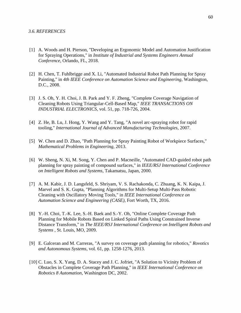
60

3.6. REFERENCES

[1] A. Woods and H. Pierson, "Developing an Ergonomic Model and Automation Justification

for Spraying Operations," in Institute of Industrial and Systems Engineers Annual

Conference, Orlando, FL, 2018.

[2] H. Chen, T. Fuhlbrigge and X. Li, "Automated Industrial Robot Path Planning for Spray

Painting," in 4th IEEE Conference on Automation Science and Engineering, Washington,

D.C., 2008.

[3] J. S. Oh, Y. H. Choi, J. B. Park and Y. F. Zheng, "Complete Coverage Navigation of

Cleaning Robots Using Triangular-Cell-Based Map," IEEE TRANSACTIONS ON

INDUSTRIAL ELECTRONICS, vol. 51, pp. 718-726, 2004.

[4] Z. He, B. Lu, J. Hong, Y. Wang and Y. Tang, "A novel arc-spraying robot for rapid

tooling," International Journal of Advanced Manufacturing Technologies, 2007.

[5] W. Chen and D. Zhao, "Path Planning for Spray Painting Robot of Workpiece Surfaces,"

Mathematical Problems in Engineering, 2013.

[6] W. Sheng, N. Xi, M. Song, Y. Chen and P. Macneille, "Automated CAD-guided robot path

planning for spray painting of compound surfaces," in IEEE/RSJ International Conference

on Intelligent Robots and Systems, Takamatsu, Japan, 2000.

[7] A. M. Kabir, J. D. Langsfeld, S. Shriyam, V. S. Rachakonda, C. Zhuang, K. N. Kaipa, J.

Marvel and S. K. Gupta, "Planning Algorithms for Multi-Setup Multi-Pass Robotic

Cleaning with Oscillatory Moving Tools," in IEEE International Conference on

Automation Science and Engineering (CASE), Fort Worth, TX, 2016.

[8] Y.-H. Choi, T.-K. Lee, S.-H. Baek and S.-Y. Oh, "Online Complete Coverage Path

Planning for Mobile Robots Based on Linked Spiral Paths Using Constrained Inverse

Distance Transform," in The IEEE/RSJ International Conference on Intelligent Robots and

Systems , St. Louis, MO, 2009.

[9] E. Galceran and M. Carreras, "A survey on coverage path planning for robotics," Rovotics

and Autonomous Systems, vol. 61, pp. 1258-1276, 2013.

[10] C. Luo, S. X. Yang, D. A. Stacey and J. C. Jofriet, "A Solution to Vicinity Problem of

Obstacles in Complete Coverage Path Planning," in IEEE International Conference on

Robotics 8 Automation, Washington DC, 2002.

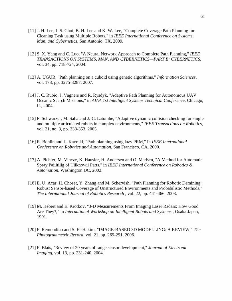
61

[11] J. H. Lee, J. S. Choi, B. H. Lee and K. W. Lee, "Complete Coverage Path Planning for

Cleaning Task using Multiple Robots," in IEEE International Conference on Systems,

Man, and Cybernetics, San Antonio, TX, 2009.

[12] S. X. Yang and C. Luo, "A Neural Network Approach to Complete Path Planning," IEEE

TRANSACTIONS ON SYSTEMS, MAN, AND CYBERNETICS—PART B: CYBERNETICS,

vol. 34, pp. 718-724, 2004.

[13] A. UGUR, "Path planning on a cuboid using genetic algorithms," Information Sciences,

vol. 178, pp. 3275-3287, 2007.

[14] J. C. Rubio, J. Vagners and R. Rysdyk, "Adaptive Path Planning for Autonomous UAV

Oceanic Search Missions," in AIAA 1st Intelligent Systems Technical Conference, Chicago,

IL, 2004.

[15] F. Schwarzer, M. Saha and J.-C. Latombe, "Adaptive dynamic collision checking for single

and multiple articulated robots in complex environments," IEEE Transactions on Robotics,

vol. 21, no. 3, pp. 338-353, 2005.

[16] R. Bohlin and L. Kavraki, "Path planning using lazy PRM," in IEEE International

Conference on Robotics and Automation, San Francisco, CA, 2000.

[17] A. Pichler, M. Vincze, K. Hausler, H. Andersen and O. Madsen, "A Method for Automatic

Spray Paiiitiiig of Uiiknowii Parts," in IEEE International Conference on Robotics &

Automation, Washington DC, 2002.

[18] E. U. Acar, H. Choset, Y. Zhang and M. Schervish, "Path Planning for Robotic Demining:

Robust Sensor-based Coverage of Unstructured Environments and Probabilistic Methods,"

The International Journal of Robotics Research , vol. 22, pp. 441-466, 2003.

[19] M. Hebert and E. Krotkov, "3-D Measurements From Imaging Laser Radars: How Good

Are They?," in International Workshop on Intelligent Robots and Systems , Osaka Japan,

1991.

[20] F. Remondino and S. El-Hakim, "IMAGE-BASED 3D MODELLING: A REVIEW," The

Photogrammetric Record, vol. 21, pp. 269-291, 2006.

[21] F. Blais, "Review of 20 years of range sensor development," Journal of Electronic

Imaging, vol. 13, pp. 231-240, 2004.

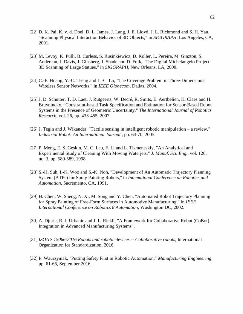
62

[22] D. K. Pai, K. v. d. Doel, D. L. James, J. Lang, J. E. Lloyd, J. L. Richmond and S. H. Yau,

"Scanning Physical Interaction Behavior of 3D Objects," in SIGGRAPH, Los Angeles, CA,

2001.

[23] M. Levoy, K. Pulli, B. Curless, S. Rusinkiewicz, D. Koller, L. Pereira, M. Ginzton, S.

Anderson, J. Davis, J. Ginsberg, J. Shade and D. Fulk, "The Digital Michelangelo Project:

3D Scanning of Large Statues," in SIGGRAPH, New Orleans, LA, 2000.

[24] C.-F. Huang, Y.-C. Tseng and L.-C. Lo, "The Coverage Problem in Three-Dimensional

Wireless Sensor Networks," in IEEE Globecom, Dallas, 2004.

[25] J. D. Schutter, T. D. Laet, J. Rutgeerts, W. Decré, R. Smits, E. Aertbeliën, K. Claes and H.

Bruyninckx, "Constraint-based Task Specification and Estimation for Sensor-Based Robot

Systems in the Presence of Geometric Uncertainty," The International Journal of Robotics

Research, vol. 26, pp. 433-455, 2007.

[26] J. Tegin and J. Wikander, "Tactile sensing in intelligent robotic manipulation – a review,"

Industrial Robot: An International Journal , pp. 64-70, 2005.

[27] P. Meng, E. S. Geskin, M. C. Leu, F. Li and L. Tismeneskiy, "An Analytical and

Experimental Study of Cleaning With Moving Waterjets," J. Manuf. Sci. Eng., vol. 120,

no. 3, pp. 580-589, 1998.

[28] S.-H. Suh, I.-K. Woo and S.-K. Noh, "Development of An Automatic Trajectory Planning

System (ATPs) for Spray Painting Robots," in Intemational Conference on Robotics and

Automation, Sacremento, CA, 1991.

[29] H. Chen, W. Sheng, N. Xi, M. Song and Y. Chen, "Automated Robot Trajectory Planning

for Spray Painting of Free-Form Surfaces in Automotive Manufacturing," in IEEE

International Conference on Robotics 8 Automation, Washington DC, 2002.

[30] A. Djuric, R. J. Urbanic and J. L. Rickli, "A Framework for Collaborative Robot (CoBot)

Integration in Advanced Manufacturing Systems".

[31] ISO/TS 15066:2016 Robots and robotic devices -- Collaborative robots, International

Organization for Standardization, 2016.

[32] P. Waurzyniak, "Putting Safety First in Robotic Automation," Manufacturing Engineering,

pp. 61-66, September 2016.

63

[33] T. Anandan, "Robotic Industry Insights: Collaborative Robots and Safety," Robotic

Inustries Association, 26 Jan 2016. [Online]. Available: https://www.robotics.org/content-

detail.cfm?content_id=5908.

[34] Universal Robots, "Afraid to Commit? No Problem, with Flexible, Redeployable Cobots,"

3 June 2016. [Online]. Available: https://blog.universal-robots.com/flexible-redeployable-

cobots. [Accessed 30 April 2017].

[35] Robotiq, "Teaching Robots Welding," [Online]. Available:

http://robotiq.com/solutions/robot-teaching/. [Accessed 6 May 2017].

[36] P. Stone and M. Veloso, "Towards collaborative and adversarial learning: a case study in

robotic soccer," International Journal of Human-Computer Studies, vol. 48, pp. 83-104,

1998.

[37] R. Mitnik, M. Recabarren, M. Nussbaum and A. Soto, "Collaborative robotic instruction: A

graph teaching experience," Computers and Education, vol. 53, pp. 330-342, 2009.

[38] S. Brown and H. Pierson, "A Collaborative Framework for Robotic Task Specification,"

Procedia Manufacturing, vol. 17, pp. 270-277, 2018.

[39] C. Connolly, "Cumulative generation of octree models from range data," in IEEE

International Conference, 1984.

[40] Roman, "Find the shortest distance between a point and line segments (not line)," August

2017. [Online]. Available: https://stackoverflow.com/questions/27161533/find-the-

shortest-distance-between-a-point-and-line-segments-not-line.

[41] D. Dakdouk, "Tool Accessibility with Path and Motion Planning for Robotic Drilling and

Riveting," Ryerson University, 2016.

[42] D. Vinayagamoorthy, "Rotor Blade," 29 Ocotober 2017. [Online]. Available:

https://grabcad.com/library/rotor-blade-8.

[43] C. Domingos, "Wing_Section_NACA23015C200," 2 January 2018. [Online]. Available:

https://grabcad.com/library/wing_section_naca23015c200-1.

[44] F. H. Macias, "rueda motriz e inducida grua viajera," 21 September 2017. [Online].

Available: https://grabcad.com/library/rueda-motriz-e-inducida-grua-viajera-1.

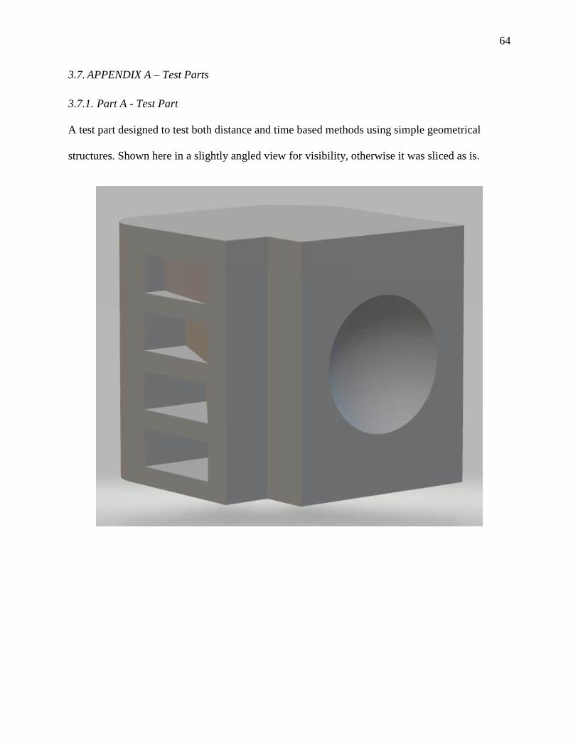
64

3.7. APPENDIX A – Test Parts

3.7.1. Part A - Test Part

A test part designed to test both distance and time based methods using simple geometrical

structures. Shown here in a slightly angled view for visibility, otherwise it was sliced as is.

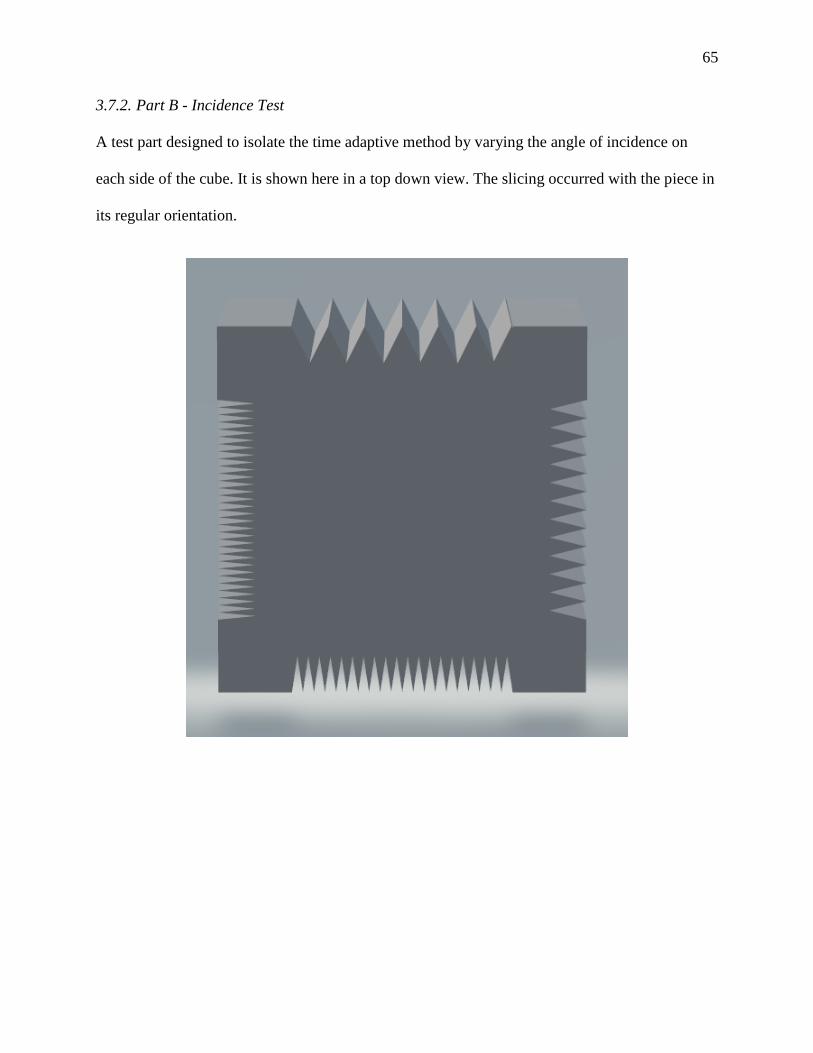
65

3.7.2. Part B - Incidence Test

A test part designed to isolate the time adaptive method by varying the angle of incidence on

each side of the cube. It is shown here in a top down view. The slicing occurred with the piece in

its regular orientation.

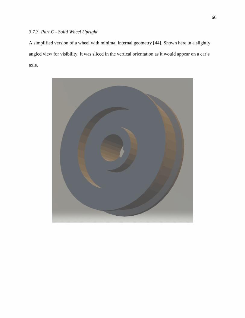
66

3.7.3. Part C - Solid Wheel Upright

A simplified version of a wheel with minimal internal geometry [44]. Shown here in a slightly

angled view for visibility. It was sliced in the vertical orientation as it would appear on a car’s

axle.

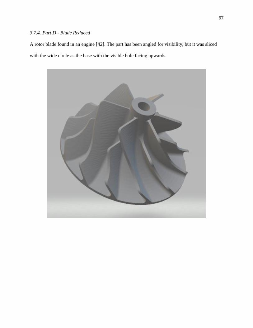
67

3.7.4. Part D - Blade Reduced

A rotor blade found in an engine [42]. The part has been angled for visibility, but it was sliced

with the wide circle as the base with the visible hole facing upwards.

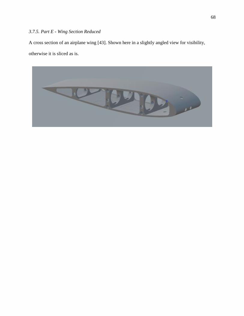
68

3.7.5. Part E - Wing Section Reduced

A cross section of an airplane wing [43]. Shown here in a slightly angled view for visibility,

otherwise it is sliced as is.

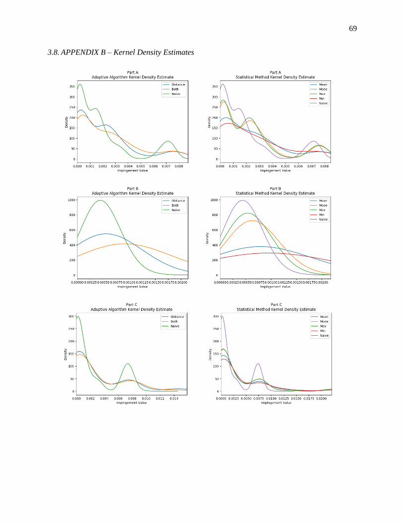
69

3.8. APPENDIX B – Kernel Density Estimates

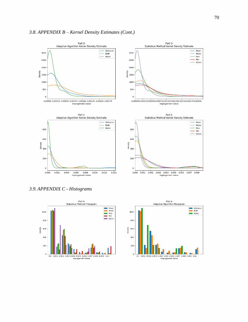
70

3.8. APPENDIX B – Kernel Density Estimates (Cont.)

3.9. APPENDIX C - Histograms

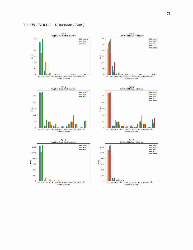
71

3.9. APPENDIX C – Histograms (Cont.)

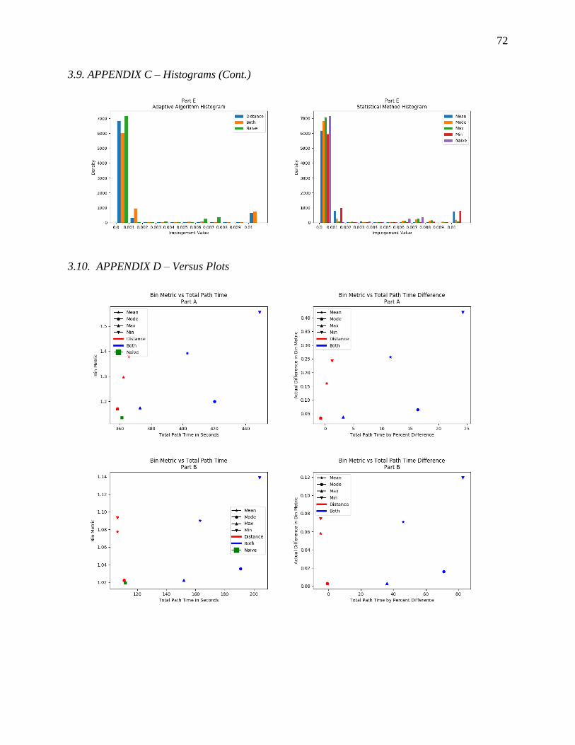
72

3.9. APPENDIX C – Histograms (Cont.)

3.10. APPENDIX D – Versus Plots

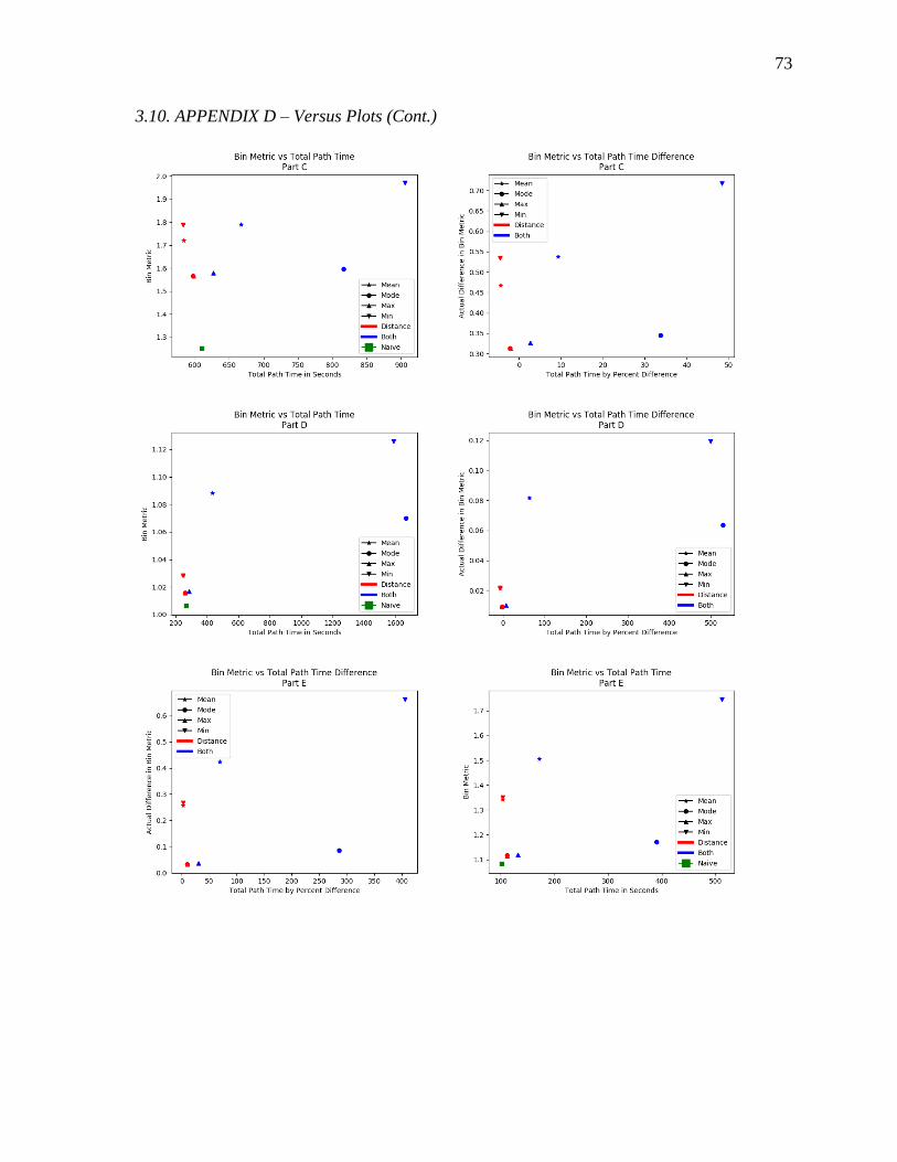
73

3.10. APPENDIX D – Versus Plots (Cont.)

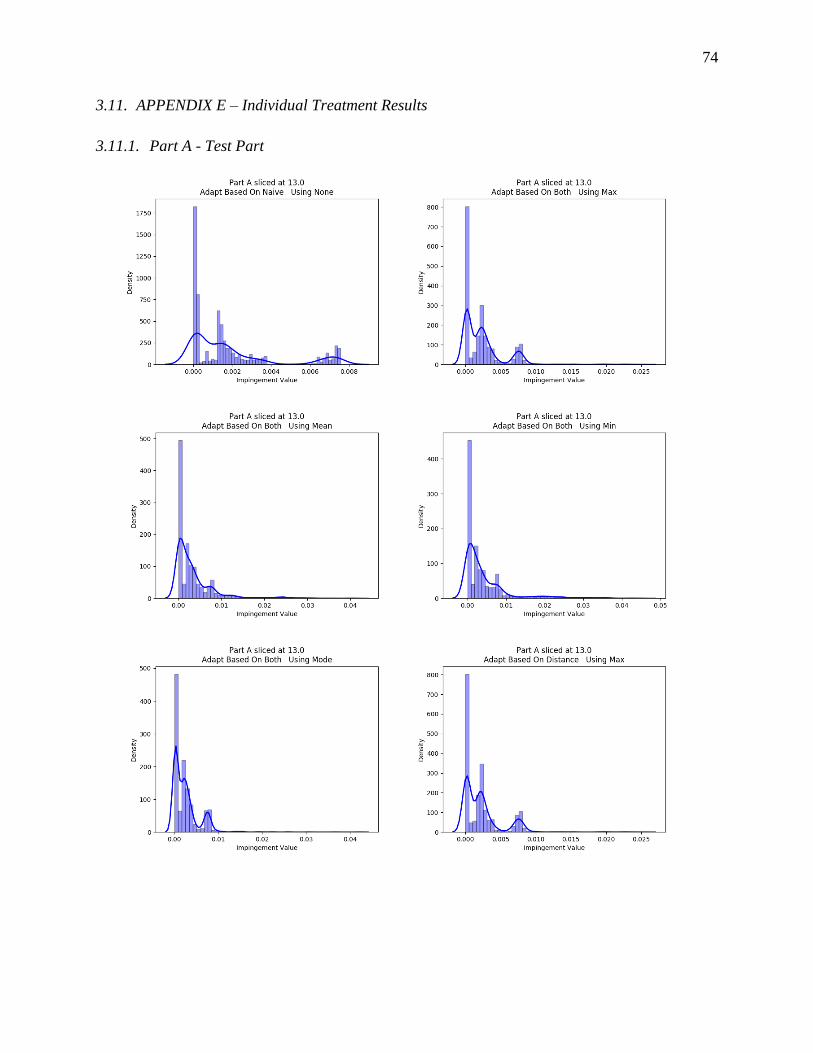
74

3.11. APPENDIX E – Individual Treatment Results

3.11.1. Part A - Test Part

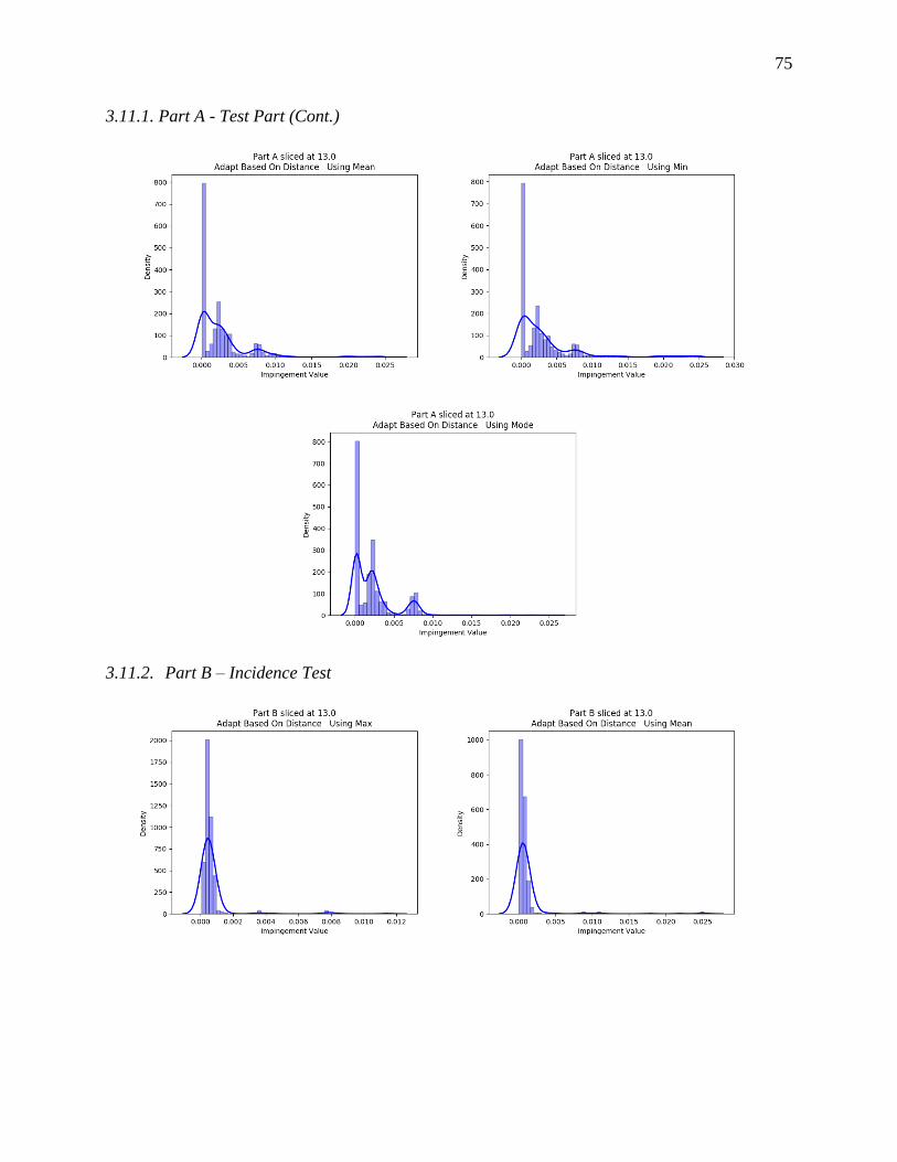
75

3.11.1. Part A - Test Part (Cont.)

3.11.2. Part B – Incidence Test

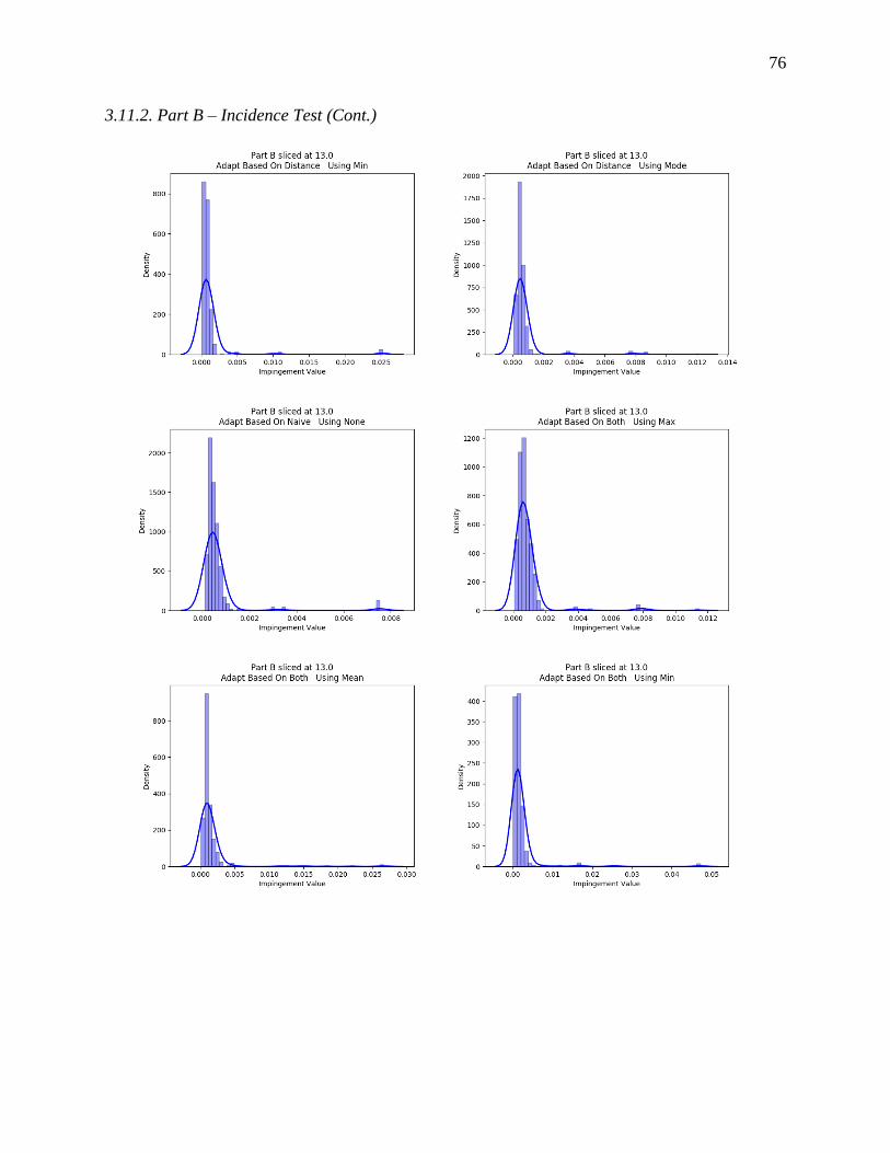
76

3.11.2. Part B – Incidence Test (Cont.)

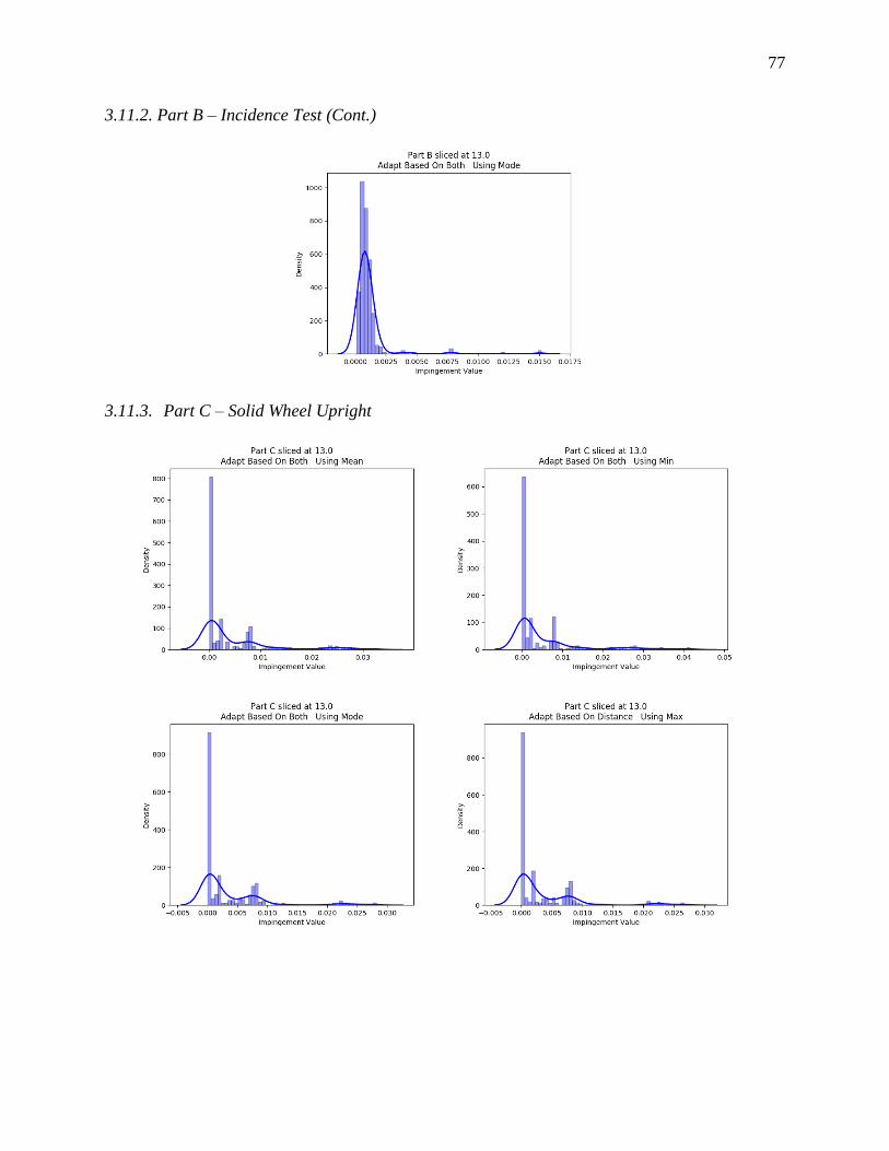
77

3.11.2. Part B – Incidence Test (Cont.)

3.11.3. Part C – Solid Wheel Upright

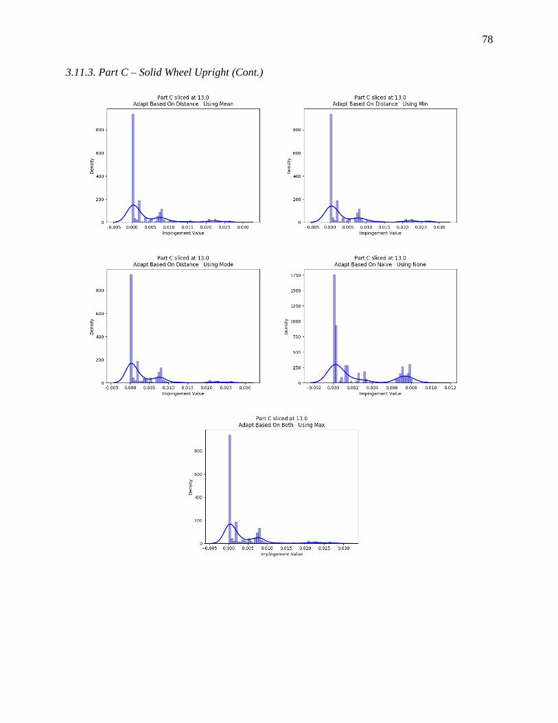
78

3.11.3. Part C – Solid Wheel Upright (Cont.)

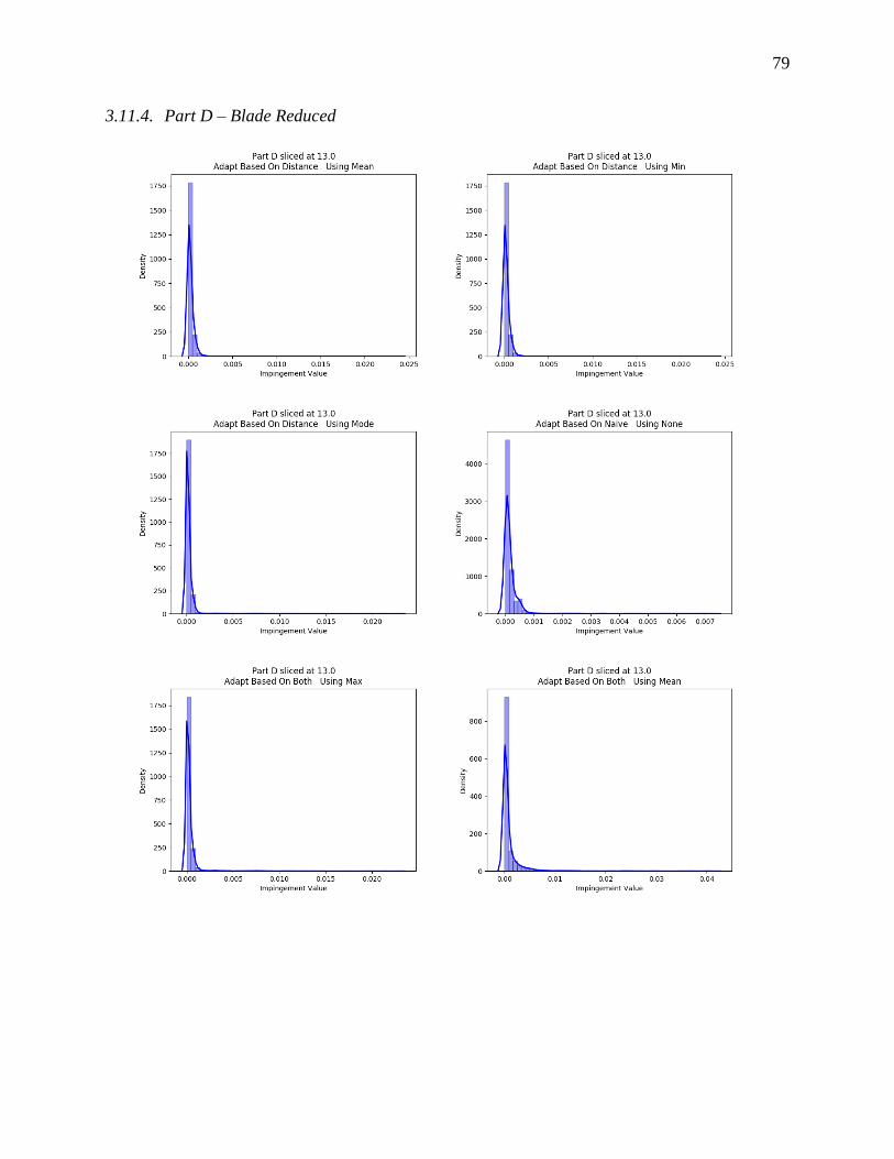
79

3.11.4. Part D – Blade Reduced

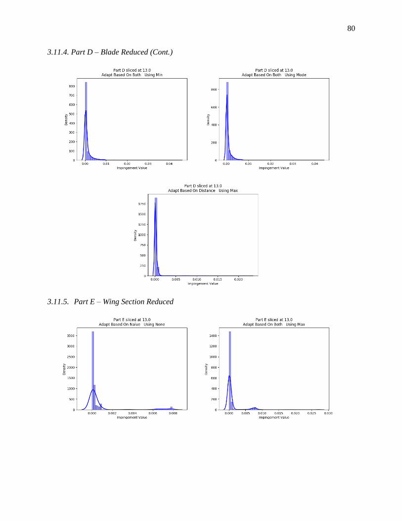
80

3.11.4. Part D – Blade Reduced (Cont.)

3.11.5. Part E – Wing Section Reduced

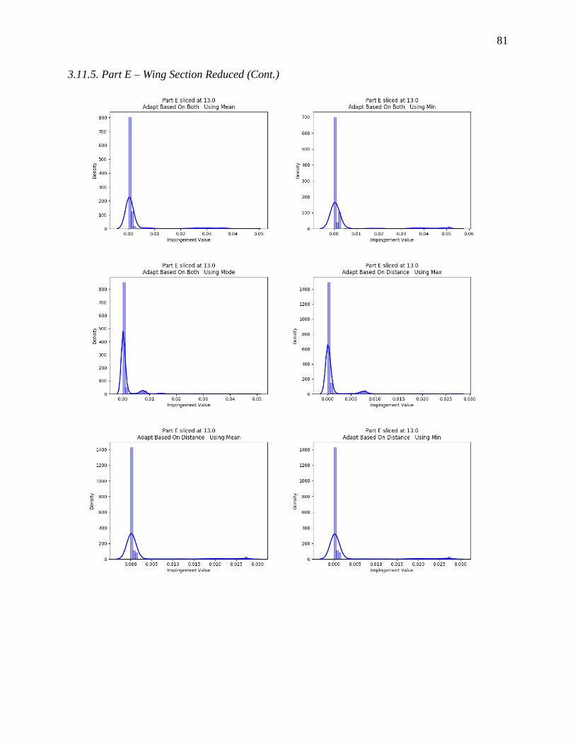
81

3.11.5. Part E – Wing Section Reduced (Cont.)

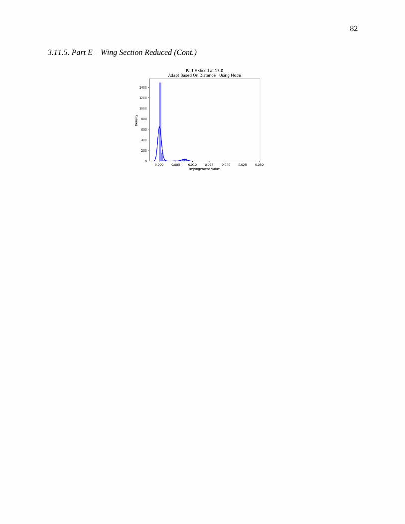
82

3.11.5. Part E – Wing Section Reduced (Cont.)

83

3.12. APPENDIX F – Nomenclature Table

𝐴 = ordered set of unique surface points a

𝒂𝑓𝑖 = intersecting surface points created from

facet f

𝐵𝑖 = set of all points mapped to bin i

𝐵𝑠 = set of all bins on slice s

�̂�𝑖 = segment normal of segment i

C = point cloud of the original part

𝐶𝑠 = point cloud points effected by slice s

c = point in the original point cloud

𝑑𝑂 = offset distance

𝑑𝐴𝐺𝑏 = aggregate distance value of all points in

bin b

𝑑𝑝 = movement distance to p

𝑒𝑓𝑖 = interpolation percentage for side i of

facet f

𝜀 = limit on angular deviation for adjacent

points

η = number of facets in a part

𝐹𝑠 = intersecting facets on slice s of the convex

hull

f = facet of the convex hull

G = robotic trajectory

g = tool trajectory observation

H = convex hull of the part

ℎ𝑠 = height of slice s

𝑙𝑖 = actual length of segment i

𝑙𝑚 = maximum allowable length of a segment

𝛾𝑐 = impingement value of point c

m = appropriate number of slices for the

convex hull or segments needed to meet

the limit 𝜀

𝑁 = set of normal vectors associated with

surface point a

�̂� = unit normal vector

P = ordered set of all path points p

𝑃𝑠 = set of all points in slice s

𝒑 = end effector position

𝒑new𝑗 = intermediary point j being added to

the path in bin

Φ𝑠 = ordered set of all points and normal

vectors in slice s

𝝓𝑓𝑖 = vector between the lone vertex and the

other two vertices

𝜑 = set of p and n

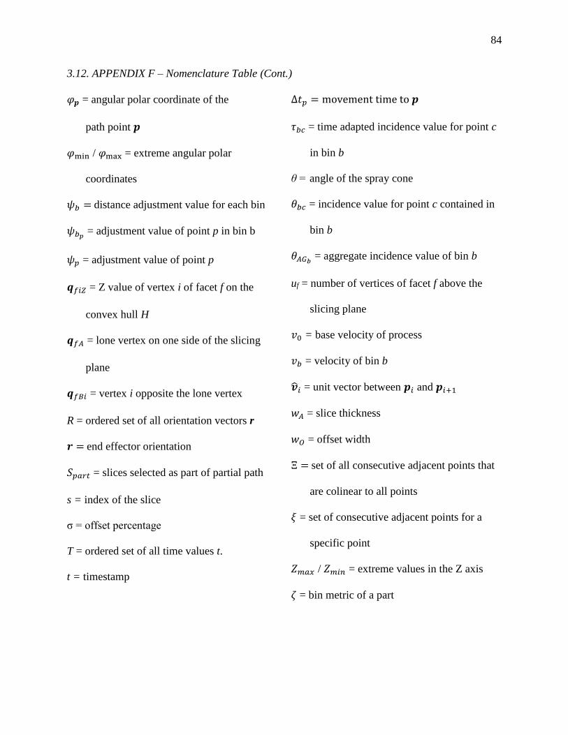
84

3.12. APPENDIX F – Nomenclature Table (Cont.)

𝜑𝒑 = angular polar coordinate of the

path point 𝒑

𝜑min / 𝜑max = extreme angular polar

coordinates

𝜓𝑏 = distance adjustment value for each bin

𝜓𝑏𝑝 = adjustment value of point p in bin b

𝜓𝑝 = adjustment value of point p

𝒒𝑓𝑖𝑍 = Z value of vertex i of facet f on the

convex hull H

𝒒𝑓𝐴 = lone vertex on one side of the slicing

plane

𝒒𝑓𝐵𝑖 = vertex i opposite the lone vertex

R = ordered set of all orientation vectors r

𝒓 = end effector orientation

𝑆𝑝𝑎𝑟𝑡 = slices selected as part of partial path

s = index of the slice

σ = offset percentage

T = ordered set of all time values t.

t = timestamp

∆𝑡𝑝 = movement time to 𝒑

𝜏𝑏𝑐 = time adapted incidence value for point c

in bin b

θ = angle of the spray cone

𝜃𝑏𝑐 = incidence value for point c contained in

bin b

𝜃𝐴𝐺𝑏 = aggregate incidence value of bin b

uf = number of vertices of facet f above the

slicing plane

𝑣0 = base velocity of process

𝑣𝑏 = velocity of bin b

�̂�𝑖 = unit vector between 𝒑𝑖 and 𝒑𝑖+1

𝑤𝐴 = slice thickness

𝑤𝑂 = offset width

Ξ = set of all consecutive adjacent points that

are colinear to all points

𝜉 = set of consecutive adjacent points for a

specific point

𝑍𝑚𝑎𝑥 / 𝑍𝑚𝑖𝑛 = extreme values in the Z axis

𝜁 = bin metric of a part

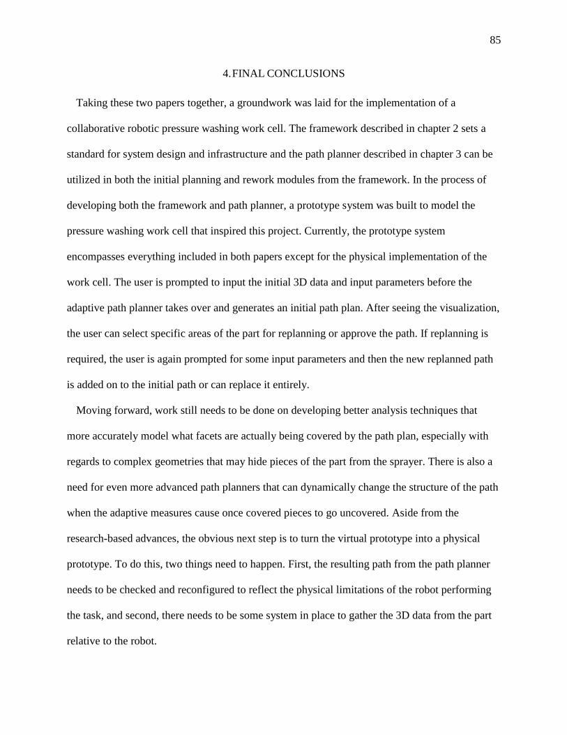
85

4. FINAL CONCLUSIONS

Taking these two papers together, a groundwork was laid for the implementation of a

collaborative robotic pressure washing work cell. The framework described in chapter 2 sets a

standard for system design and infrastructure and the path planner described in chapter 3 can be

utilized in both the initial planning and rework modules from the framework. In the process of

developing both the framework and path planner, a prototype system was built to model the

pressure washing work cell that inspired this project. Currently, the prototype system

encompasses everything included in both papers except for the physical implementation of the

work cell. The user is prompted to input the initial 3D data and input parameters before the

adaptive path planner takes over and generates an initial path plan. After seeing the visualization,

the user can select specific areas of the part for replanning or approve the path. If replanning is

required, the user is again prompted for some input parameters and then the new replanned path

is added on to the initial path or can replace it entirely.

Moving forward, work still needs to be done on developing better analysis techniques that

more accurately model what facets are actually being covered by the path plan, especially with

regards to complex geometries that may hide pieces of the part from the sprayer. There is also a

need for even more advanced path planners that can dynamically change the structure of the path

when the adaptive measures cause once covered pieces to go uncovered. Aside from the

research-based advances, the obvious next step is to turn the virtual prototype into a physical

prototype. To do this, two things need to happen. First, the resulting path from the path planner

needs to be checked and reconfigured to reflect the physical limitations of the robot performing

the task, and second, there needs to be some system in place to gather the 3D data from the part

relative to the robot.

86

In summary, the Army’s need to remove operators from the pressure washing work cell led to

the creation of a collaborative task specification system designed to handle a wide variety of

novel parts requiring reliable one-off path planning, which in turn led to the development of an

adaptive path planning algorithm for better quality toolpaths.