Collection Efficiency and Ice Accretion Calculations … Efficiency and Ice Accretion Calculations for a Boeing 737-300 Inlet Colin S. Bidwell National Aeronautics and Space Administration

NASA Technical Memorandum 107347

/,,'U_--o

C3-'_-- ' / C?_

Collection Efficiency and Ice Accretion

Calculations for a Boeing 737-300 Inlet

Colin S. Bidwell

Lewis Research Center

Cleveland, Ohio

Prepared for the

World Aviation Congress

cosponsored by the Society of Automotive Engineers and the

American Institute for Aeronautics and Astronautics

Los Angeles, California, October 22-24, 1996

National Aeronautics and

Space Administration

https://ntrs.nasa.gov/search.jsp?R=19970013640 2018-07-12T18:24:48+00:00Z

Collection Efficiency and Ice Accretion Calculations for a

Boeing 737-300 Inlet

Colin S. Bidwell

National Aeronautics and Space Administration


Cleveland, Ohio 44135

SUMMARY

Collection efficiency and ice accretion calculations have been made for a Boeing 737-300

inlet using a three-dimensional panel code, an adaptive grid code, the NASA Lewis LEWICE3D

grid based ice accretion code. Flow solutions for the inlet were generated using the VSAERO

panel code. Grids used in the ice accretion calculations were generated using the newly developed

adaptive grid code ICEGRID3D. The LEWICE3D grid based ice accretion program was used to

calculate impingement efficiency and ice shapes. Ice shapes typifying rime and mixed icing con-

ditions were generated for a 30 minute hold condition. All calculations were performed on an SGI

Power Challenge computer. The results have been compared to experimental flow and impinge-

ment data. In general, the calculated flow and collection efficiencies compared well with experi-

ment, and the ice shapes looked reasonable and appeared representative of the rime and mixed

icing conditions for which they were calculated.

NOMENCLATURE

d

HTC

LWC

MVD

W

fx

0

Droplet diameter, _tmConvective heat transfer coefficient, W/m2/K

Liquid Water Content, g/m 3

Median Volume Diameter, lain

Mass flow, kg/s

Collection efficiency

Angle-of-attack, degrees

Radial angle around inlet lip measured from the upper inlet lip, degrees

I. INTRODUCTION

The last 15 years has brought great changes in the computer software and hardware indus-

try, changes which have given the design engineer a larger more sophisticated set of tools. A lit-

eral explosion of software has effected every level and aspect of engineering design. Engineers

now have quick, and accurate tools at their fingertips to handle just about any design task imagin-

able. Tasks that were once unmanageable or manageable only by small Computational Fluid

Dynamic (CFD) groups on expensive machines are now tractable by the ordinary design engineer.

Computer programs that once took 10 hours of computer time and 2 days of turnaround time can

now be done overnight on powerful, inexpensive workstations..Design tasks that were once

empirically based "arts" are now analytically based sciences. One such area that has benefitted

greatly from these changes has been the design of aircraft ice protection systems.

The task of aircraft ice protection system design which was previously one of subjectivity,

based heavily on correlation and extrapolation, and carried out by highly experienced individuals

is now one of objectivity, based on sound models and carded out by entry level engineers. Histor-

ically systems have been designed using the methods of ADS-4 (ref. 1). This entailed interpola-

tion or extrapolating from previously tested conditions and configurations. If a configuration or

condition didn't exist in ADS-4 then various forms of extrapolation were used. As the aircraft

industry progressed the newer designs were less and less similar to those in the ADS-4 database

and the task of interpolation or extrapolation became harder and riskier. With the advent of the

computer age numerical methods were made available, reducing the guess work. Many 2D and

some 3D methods are now available to aid the user in designing an aircraft ice protection system

(ref. 2-6). This paper outlines one such 3D method and presents validation for a Boeing 737-300inlet.

Flow, trajectory and ice accretion calculations were made and compared to experiment for

the Boeing 737-300 inlet using the VSAERO flow solver (ref. 7), the 3D adaptive grid code

ICEGRID3D and the grid based NASA Lewis 3D ice accretion code LEWlCE3D (ref. 6). The

cases were chosen to illustrate the flexibility and to provide validation for the computer code.

The grid based LEWlCE3D code is very similar to the panel based version and incorpo-

rates the same trajectory and ice accretion methodology. The codes are different, in that the grid

based code does not incorporate a flow solver but is dependent on the user to supply one. Several

advantages of this are the ability to handle a users particular flow solver and the fact that the grid

based trajectory codes are significantly faster than the panel based trajectory codes. The code can

handle generic multi-block, structured or unstructured grids, simple cartesian grids and adaptive

grids with symmetry planes. Performance differences can be as high 200 to 1 between the panel

and grid based methods with a typical grid based case (single section of interest, single drop size)

taking about 2.5 minutes on an SGI Power Challenge computer.

Computational and experimental results are presented for flow, and collection efficiency

for a Boeing 737-300 inlet. All of the flow calculations were made using the VSAERO flow

solver. All of the aerodynamic and collection efficiency data were taken in 1985 in the NASA

Lewis Icing Research Tunnel (IRT) under a program funded by NASA and the FAA and carried

out by Wichita State University, Boeing Military Airplanes and NASA (ref. 8).

H. EXPERIMENT

A. EXPERIMENTAL APPARATUS

The aerodynamic and impingement efficiency tests were carried out in the NASA Lewis

IRT. The test equipment included the IRT (fig. 1), the ESCORT data system, a special spray sys-

tem for the impingement tests (fig. 2), a laser reflectometer for impingement efficiency data reduc-

tion (fig. 3), and the Boeing 737-300 inlet model (fig. 4).

The IRT facility can provide a range of airspeeds, angles-of-attack, temperatures, liquid

water contents (LWC), and drop sizes (ref. 9). The IRT has a 2.47 m x 1.82 m test section with a

maximum airspeed of 134 m/s (empty tunnel). Angle-of-attack is controlled by a movable turnta-

ble to which the models are mounted. A refrigeration system allows year-round testing at temper-

atures from -29 ° C to 10 ° C. The spray system located upstream of the test section can provide a

cloud with a range of LWC of .25-3.0 grn/m 3 and a median volume drop (MVD) size range of 12-

40 _tm.

The Escort system was developed at Lewis to aid in storage, processing, and analysis of

large amounts of data (e.g. temperature, pressure) produced in various experiments at Lewis

Research Center. In this test Escort was used to store tunnel total temperature, total pressure, free

stream airspeed, surface pressure, produce real time calculations and display pertinent parameters.

The storage sequence for each data point was initiated by the researcher in the control room. A

separate program was used to do a more complete post run analysis.

The spray requirements for the impingement tests precipitated the need for a different

spray system (fig. 2) than was available in the IRT (ref. 8). The IRT spray system could not pro-

duce the short (2-5 seconds), stable sprays (i.e. constant LWC and drop size) required to prevent

blotter strip saturation. There were also concerns that the dye would contaminate the IRT spray

system. The new system consisted of 12 nozzles and a supply tank located at the IRT spray bar

station (fig. 2). The system featured short supply lines which enabled short, stable sprays.

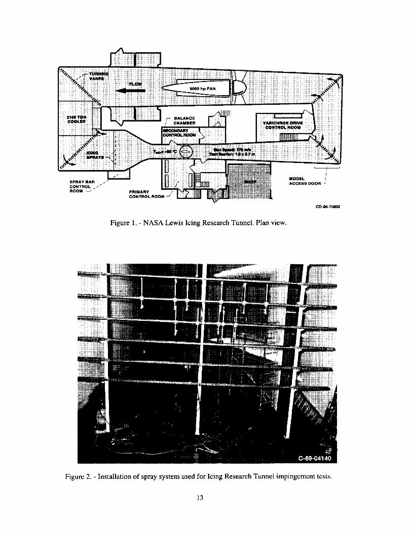
One unique feature of the current technique is the laser reflectometer used to determine

the local collection efficiency (fig. 3). The device measures the local reflectance of the blotter strip

and correlates this to the local collection efficiency (ref. 8). The device saved considerable time in

the data reduction of the blotter strips.

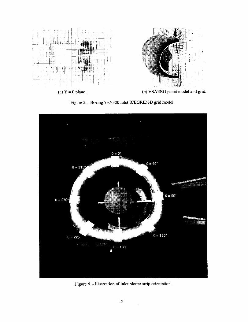
The Boeing 737-300 inlet model (fig. 4) was .2547 scale and had a conical centerbody.

The model was provided by Boeing Commercial Airplane Company. The Boeing 737-300 was

outfitted with 88 static pressure taps. The taps were located along 5 radial cuts: 0 = 0 °, 45 °, 90 °,

135 ° and 180" (fig. 5).

B. EXPERIMENTAL TESTING

Two types of testing were done in the IRT: aeroperformance and impingement efficiency

testing. The aero-performance testing involved taking surface pressure measurements. The

impingement efficiency testing involved the use of a dye tracer technique to measure the location

and amount of water impinging on the model.

Surface pressures were measured on the inlet models using the ESCORT system. Pressure

measurements were taken at an airspeed of 77 m/s, at angles-of-attack of 0 ° and 15 ° and inlet

mass flows of 7.8 kg/s and 10.4 kg/s with the spray system off. Three sets of pressure measure-

ments were taken for each configuration to establish repeatability of the data. These pressure mea-

surements were used to generate surface Mach numbers for the comparisons presented in this

paper.

The experimental technique used in the current tests to determine the impingement char-

acteristics of a body is one that was developed on the early 1950's with a few modifications (ref.

8). The technique involved spraying a dye-water solution of a known concentration onto a model

covered with blotter strips. Figure 6 shows a typical blotter installation for the 737-300 inlet. The

result was that the local impingement efficiency rate was reflected on the blotter strips as a varia-

tion in color intensity. That is, the areas of higher impingement rate are darker and those with

lower impingement rate are lighter.

Several steps were necessary to prepare the IRT for impingement testing. The specially

designed spray system had to be installed and adjusted to produce a uniform cloud. The local

LWC had to measured at each blotter strip location (with the tunnel empty) for every spray and

tunnel condition to account for any cloud nonuniformity that existed after the final spray adjust-

ment. After these adjustments and measurements were made the model was inserted and tested.

Each points was repeated five times to obtain a statistical average (ref. 8).

A typical test point for involved several steps. The model was cleaned and blotter strips

were attached at points of interest. Figure 6 shows a typical blotter strip installation for the 737-

300 inlet and illustrates the angular reference system used in presenting the data.The spray was

then made, the blotter strips were removed, and labeled, and the model was cleaned and made

ready for the next condition.

The Boeing 737-300 inlet model was tested for two drop sizes (16.45 grn, 20.36 _tm), at

two angles-of-attack (0 °, 15 °) and at two mass flows (7.8 kg/s, 10.4 kg/s). The drop size tests were

repeated three times for each condition to generate a statistical average. This resulted in a large

amount of data (-216 strips).

II. ANALYTICAL METHOD

The icing calculation required a three step process. All of the calculations were made on a

a single SGI Power Challenge computer processor (R8000). The ICEGRID3D code was used to

generate the grid for the trajectory calculations. The VSAERO code was used to generate the

velocitieson this grid and to generate the surface velocities needed in the LEWICE3D code. The

LEWICE3D code then used the panel model the surface velocity information and the grid to make

the ice accretion calculations. The LEWICE3D panel based computer program has been used in

previous calculations of isolated, finite wings and full aircraft (ref. 10-14). The work presented

here represents the first calculations made using the adaptive grid code (ICEGRID3D).

A. ICEGRID3D

The ICEGRID3D was developed at Lewis Research Center by Bidwell and Coirier specif-

ically for the task of optimizing trajectory calculations in the LEWICE3D code. The program

automatically produces grids which are optimal for trajectory calculations hence reducing the

required effort to produce a "good" trajectory grid. The program also produces a minimum of grid

points which reduces the panel code calculation times. The program requires the surface geometry

and an input file describing the grid volume and refinement parameters. The code refines the grid

near regions of interest which can include the geometry, parts of the geometry, and lines or points

input by the user. The code is similar to an oct-tree method (ref. 15) in that it recursively divides

the original grid volume until the refinement criteria for each cell has been met. The code will not

refine cells internal to the geometry. The code is different from most oct-tree methods in that the

grid volume is allowed to be multiply skewed, multiblock and different refinement functions can

be used in any direction. This last feature is where the code really differs from the oct-tree meth-

ods in that it allows a given cell to be divided into 8, 4 or 2 cells depending on the refinement

function instead of the oct-tree method which divides a cell into 8 cells if the refinement is

required. This results in grids with much fewer cells for cases where gridding requirements are

disparate in the different directions (e.g. swept wings which have a much smaller cell size require-

ment in the chordwise direction than in the spanwise direction).

The grid used in the icing calculations is shown in figure 5. The grid contains 138,098

cells and 160,047 points. The grid plane at y = 0 shows the major features of the grid. Two refine-

ment functions were chosen for the grid in each direction. The first refinement function was based

on distance from the surface. The user specifies a minimum cell size near the surface, the geomet-

ric rate of growth of the cell size as the distance from the body increases, and the maximum cell

size far away from the body. Because of the highly 3D nature of the inlet and the fact that trajec-

tory calculations were required everywhere, the refinement parameters in the x, y, and z directions

were set to be the same. The minimum x, y, and z cell size near the surface was set to 2.54 cm.

The geometric growth rate of the cells was chosen to be 1.4. The maximum x, y, and z cell size far

from the body was chosen to be 12.7 cm. The second refinement function was based on distance

from the leading edge of the inlet. This area is where most of the trajectories were to be calculated

and where the velocity gradients were the highest, hence, smaller grid spacing was required. As

for the first function, the user specifies a minimum cell size near the surface, the geometric rate of

growth of the cell size as the distance from the body increases, and the maximum cell size far

away from the body. Additionally, the user specifies the region of panels on the surface for which

the refinement is to be applied (i.e. the range of panel columns and rows of the surface patch). The

minimum x, y, and z cell size near the surface was set to 1.27cm. The geometric growth rate of the

cells was chosen to be 1.4. The maximum x, y, and z cell size far from the body was chosen to be

12.7 cm. It took approximately 5 hours of CPU time to generate this grid.

B. VSAERO

VSAERO is a first order 3D potential flow panel code (ref. 7). Geometries are represented

as quadrilaterals which have constant doublet and source distribution. The formulation used in

VSAERO results in a solution that is second order accurate allowing for accurate flow solutions

with fewer panels and less CPU time than other first order methods. The disadvantage of this

method is that because a numerical differentiation is used to generate the velocity distribution

careful panelling is required to prevent numerical errors. The code can generate solutions for

internal and external compressible flows and can handle very large problems (~10,000 panels).

For the current study, VSAERO was run using a steady, isolated inlet flow with a y = 0

plane of symmetry (fig. 4,5). The inlet model contained 1,692 panels. Flow solutions were run for

two angles-of-attack (0 °, 15 °) at two mass flows (7.8 kg/s and 10.2 kg/s). The flows solutions and

velocity calculations took approximately 85 minutes for each of the cases.

C. LEWICE3D

The LEWICE3D grid based code incorporates trajectory, heat transfer and ice shape cal-

culation into a single computer program. The code can handle generic multiblock structured grid

based flow solutions, unstructured grid based flow solutions, simple cartesian grids with surface

patches, and adaptive grids with surface patches. The latter two methods allow the use of generic

panel code input which is a computationally efficient method for generating ice shapes.The code

can handle overlapping and internal grids and can handle multiple planes of symmetry. Calcula-

tions of arbitrary streamlines and trajectories are possible. The code has the capability to calculate

tangent trajectories and impingement efficiencies for single droplets or droplet distributions. Ice

accretions can be calculated at arbitrary regions of interest in either a surface normal or tangent

trajectory direction.

The methodology used in the LEWICE3D (ref. 6) analysis can be broken into six basic

steps for each section of interest at each time step. In the first step, the flow field is generated by

the user. Secondly, surface streamlines are calculated. The surface streamline analysis uses a vari-

able step size fourth-order Runge-Kutta integration scheme developed by Bidwell (ref. 6).

Thirdly, tangent trajectories are calculated at the region of interest. An array of particles is

released between the tangent trajectories in the fourth step. These impacting particles are used to

calculate collection efficiency as a function of surface position. The trajectory analysis is basically

that of Hillyer Norment (ref. 16) with modifications by Bidwell (ref. 6). At the heart of the trajec-

tory analysis is the variable step predictor-corrector integration scheme by Krogh (ref. 17). The

fifth step involves interpolating or extrapolating the collection efficiencies onto the streamlines. In

the sixth step the ice accretion for the streamline is calculated. The ice accretion model is basi-

cally that of the LEWlCE2D code applied along surface streamlines (ref. 3).

LEWlCE3D calculation times varied for the different cases depending upon the drop size

and the number of trajectories. The LEWlCE3D calculation times are heavily dependent upon

grid size and structure because the largest portion of the LEWlCE3D calculation time (greater

than 99%) is spent calculating velocities at specified points, which involves searching through the

grid tree structure for the cell in which the point is located. The trajectory integration time for the

cases varied from .2-.5 seconds. Approximately 100 trajectories were required for each drop sizeat each section-of-interest for the ice accretion calculations. This resulted in calculation times of

approximately 1000 seconds for the inlet cases (5 sections-of-interest, 7 bin distribution). The col-

lection efficiency calculations for the entire inlet depicted in figures 9-12 required quite a few

more trajectories. A 200 x 400 matrix of particles was released for each drop size in the distribu-

tion. For each case then 560,000 trajectories were calculated resulting in run times of about 40hours.

HI. ANALYSIS

Surface velocity, heat transfer, collection efficiency, and ice shapes results are presented

for the Boeing 737-300 inlet. Ice shape calculations were made for two icing conditions simulat-

ing a rime and a mixed condition. Comparisons to experimental collection efficiency are made for

all of the cases and to experimental surface mach number or coefficient of pressure where avail-

able. Discussions of the icing conditions chosen, the LEWICE3D program parameters used, and

of the individual analysis are given below.

Two icing conditions were calculated for each data point in the collection efficiency

matrix (i.e. 2 drop sizes x 2 mass flows x 2 angles-of-attack) for the Boeing 737-300 inlet. The

icing conditions were chosen to loosely match a rime and a mixed hold condition. For the rime

condition an icing time of 30 minutes, an LWC of .2 g/m 3 and a temperature of 243.1 K were

used. For the mixed condition an icing time of 30 minutes, an LWC of .695 g/m 3 and a tempera-

ture of 263.7 K were used.

The grid based LEWICE3D computer program parameters were chosen from experience,

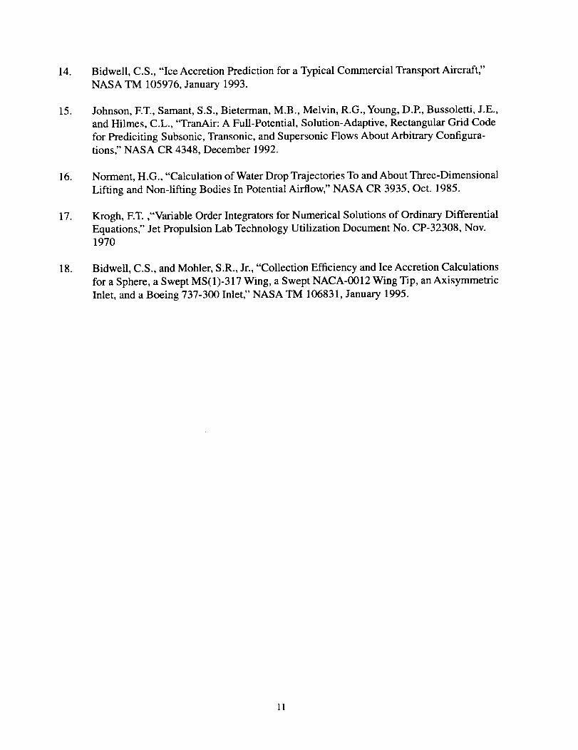
correlations and a desire to limit the computational resources required. A 7 bin experimentally

measured droplet distribution (ref. 8) was used for the calculations (table I). The icing calculations

were made using a single ice accretion time step. A LEWICE roughness parameter (ref. 3) of.5mm was used for all of the cases.

The results for the 737-300 inlet are shown in figures 7-18.The ice shape and parameter

plots were made along radial cuts parallel to the flow direction.

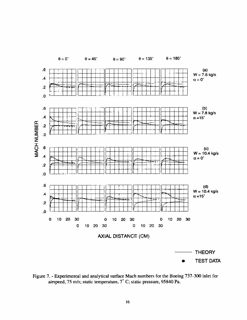
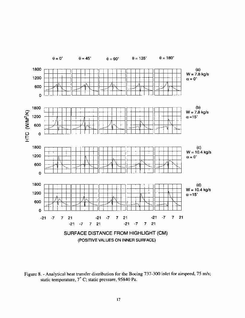
The surface mach number and heat transfer distributions are presented in figures 7, 8. In

general, the agreement between the experimental and computed surface mach number is excel-

lent. Although no experimental data was available for the heat transfer distributions, the analytical

results appear reasonable in that they follow trends set by the surface mach number distributions

(i.e where there are high mach numbers there are high heat transfer coefficients).

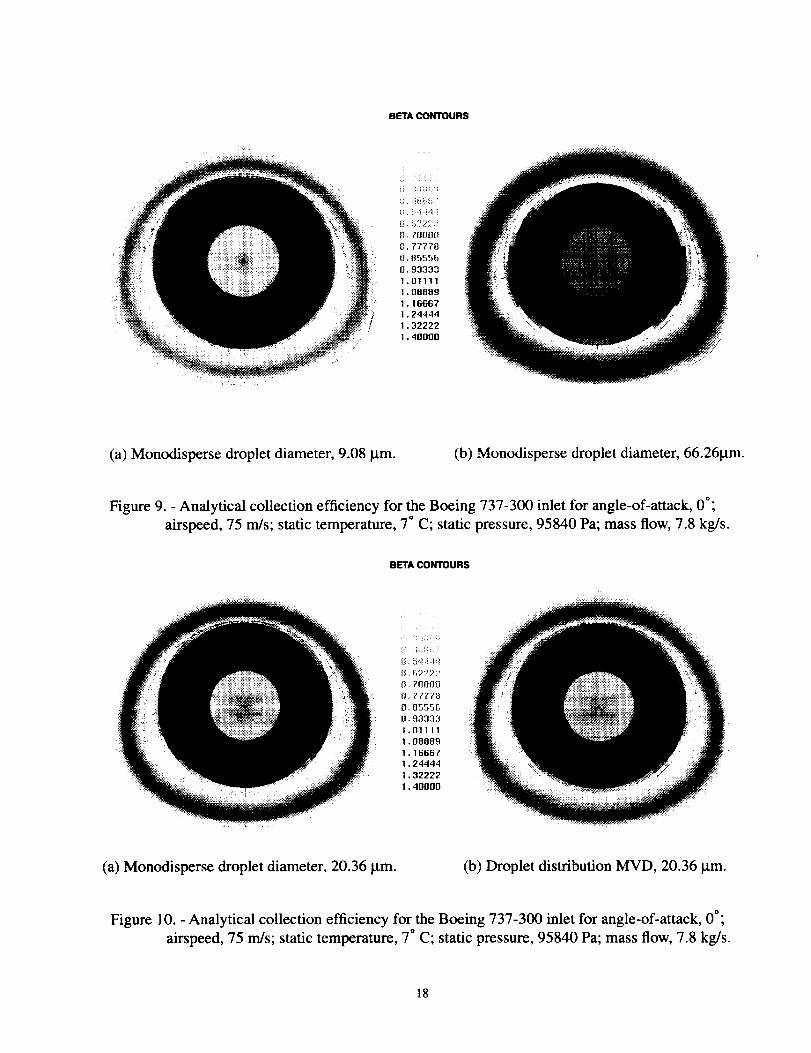
Figures 9-12 depict the overall picture of the collection efficiency for the inlet. The calculations

were generated by using a large matrix of particles (200 x 400). The calculations although expen-

sive (-6 hours) give a much broader picture of the collection efficiency characteristics of the inlet.

The effect of drop size on collection efficiency can be seen in figure 9. Increasing the drop

size results in a higher collection efficiency on the lip and centerbody of the inlet. Increasing the

drop sizealsoresultsin a lessuniformcollectionefficiencydistributionat the compressor face

with larger peak values and larger shadow zones (i.e. areas where no droplets impact). This is

because the more massive drops could not follow the flow around the inlet lip.

The effect of droplet distribution can be seen in figure 10. The droplet distribution case

yields smaller peak collection efficiencies on the inlet lip with a larger extent of impingement. The

collection efficiencies on the centerbody are larger for the distribution case. For the compressor

face the monodisperse case generates larger collection efficiencies with a greater degree of unifor-

mity.

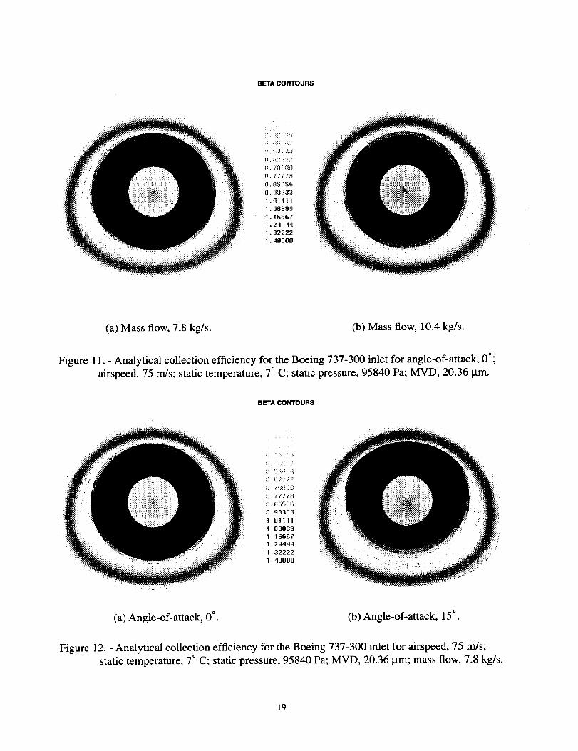
Figure 11 illustrates the effect of mass flow on the collection efficiency of the inlet. The

effect of increasing mass flow is to increases the amount of shadowing and nonuniformity on the

compressor face. Increasing the mass flow moves the maximum collection efficiency on the inlet

lip more towards the outside of the inlet.

Figure 12 illustrates the effect of increasing angle-of-attack on the collection efficiency of

the inlet. Increasing the angle-of-attack results in the peak collection efficiency moving more

towards the inside of the upper lip and more towards outside on the lower lip. The collection effi-

ciency for the right and left lips appear unaffected by changes in angle-of-attack. Increasing the

angle-of-attack results in a higher nonuniformity with higher peaks on the compressor face.

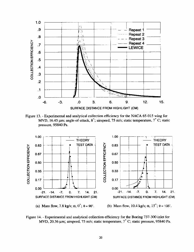
Figures 13-16 illustrate the collection efficiency comparisons between experiment and cal-

culation. The largest problem in validating trajectory codes using experimental impingement data

is defining favorable agreement. The evaluation process is at best subjective for two reasons. First,

it is difficult to generate an exact experimental curve because the impingement data is statistical in

nature and because only a small number of samples are taken (3-5) for each test condition. Sec-

ondly, the insensitivity of the method to small amounts of dye makes the exact determination of

impingement limits difficult. In judging the quality of the comparisons the following criteria are

used:

a) agreement in the general shape of curves

b) the analytical curve position within the experimental repeatability band

c) agreement in the location and size of the maximum collection efficiency

d) agreement of the impingement limits

For any given comparison one or more of these criteria may be satisfied. The impingement limits

may not match well but the maximum collection efficiency is close. The shape of the curve is

close but the maximum collection efficiency might not match. The experimental repeatability

must be taken into count when making these judgements. Figure 13 shows a typical collection

efficiency comparison between prediction and experiment for a NACA 65-015 wing. If we were

to compare the calculation to any of the repeats or to the average of the repeats in figure 13 we

would find the comparisons reasonable but not excellent. But if the experimental repeatability is

taken into account the comparisons look good except for the impingement limits. This is a typical

result (ref. 8, 18). This could be due to insufficiencies in the flow code, the trajectory codes or in

the experimental technique.

Figure 14depictstherangeof qualityof the comparisons. Figure 14a represents about the

best comparison for the inlet while figure 14b represents about the worst comparison. For both

curves the general shape of the predicted curve is correct. For figure 14a the comparison is good

everywhere except for the maximum collection efficiency. The code slightly underpredicts the

maximum collection efficiency. For figure 14b the agreement is good for the upper surface and for

the maximum collection efficiency. The agreement deteriorates on the underside of the wing

where the code overpredicts the collection efficiency and the lower impingement limit. If the

experimental repeatability were taken into account the comparison would improve slightly.

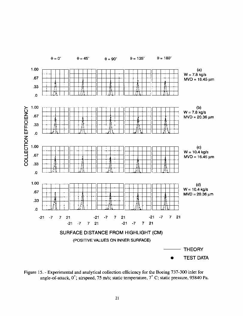
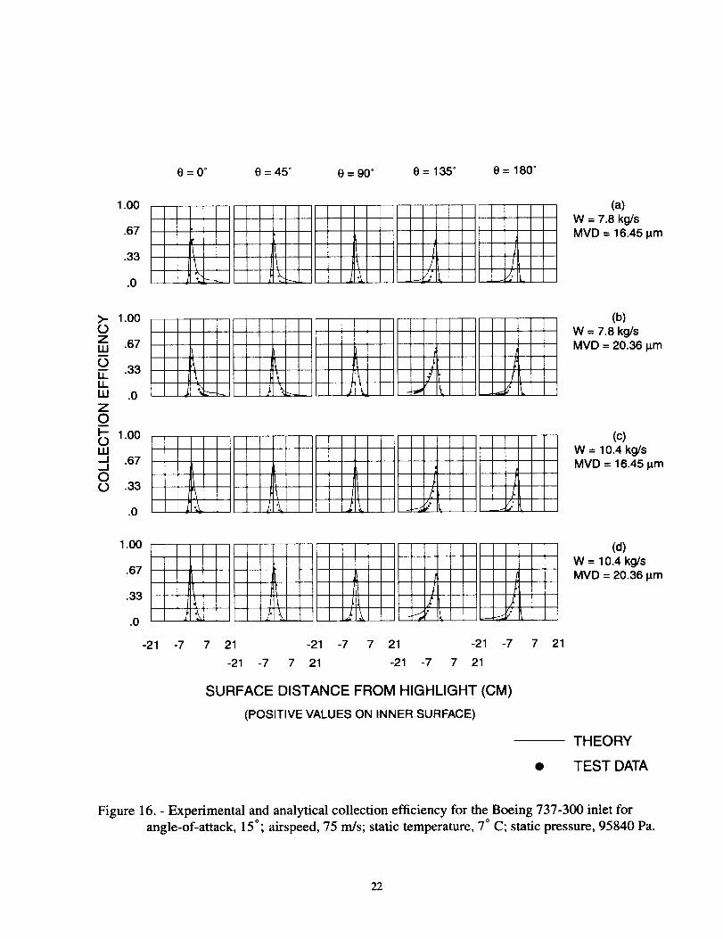
Figure 15,16 show the overall comparison of experiment and calculation. On average, the

agreement is good. The experimental and computational results agree well in shape of curve, area

under the curve, maximum collection efficiency and impingements limit for the most part.

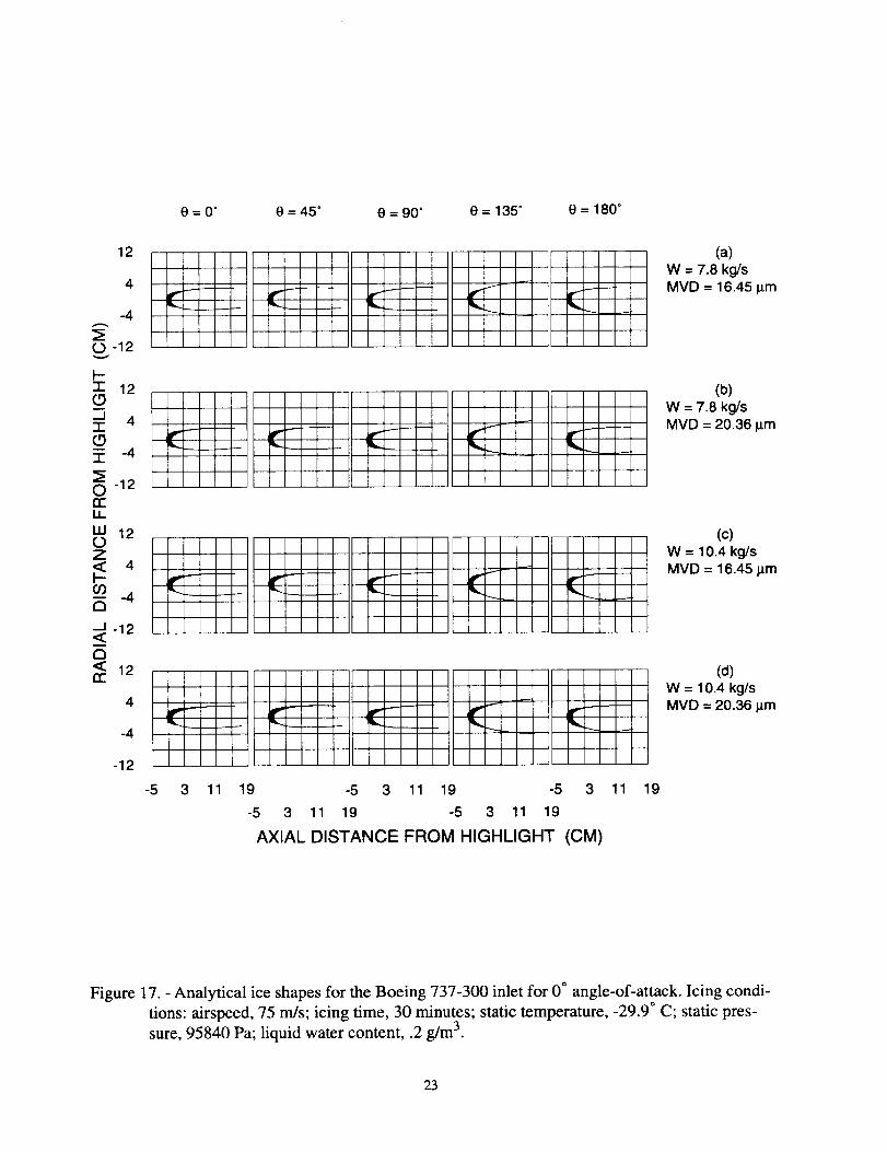
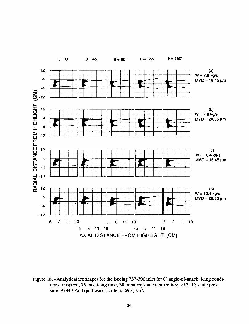
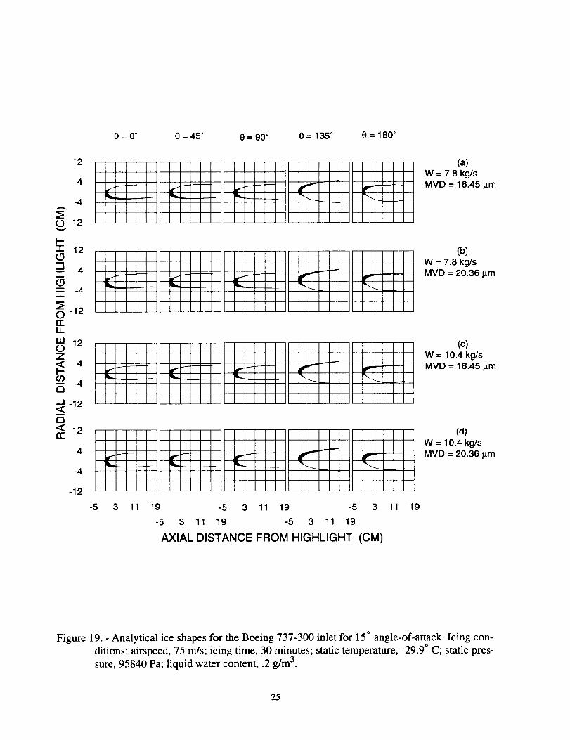
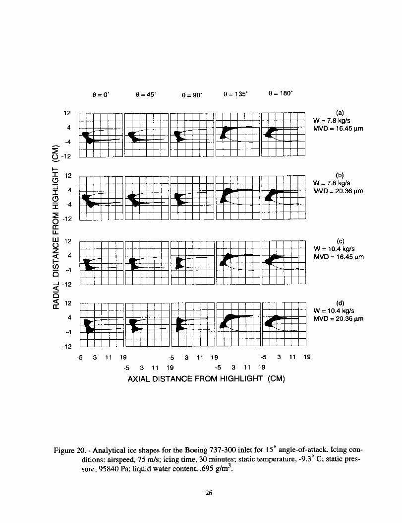
The computed ice shapes are presented in figures 17-20. Although no experimental data

was available the results looked consistent with the conditions for which the shapes were gener-

ated, and with the collection efficiency distribution and with the heat transfer distribution. At a

given positive inlet angle-of-attack the ice shape transitions from more towards the outside of the

inlet to more towards the inside of the inlet as we traverse from the lower lip around the inlet to

the upper lip. For a given inlet angle-of-attack increasing the mass flow results in an ice shape thatis more towards the outside of the inlet.

V. CONCLUSION

The grid based LEWICE3D-VSAERO-ICEGRID3D combination proved to be an inex-

pensive, flexible, accurate ice protection system design tool. The flow and ice accretion calcula-

tions were done quickly, cheaply and accurately for a range of 3D conditions.

The ICEGRID3D, VSAERO, grid based LEWlCE3D, combination was, in general, inex-

pensive to operate. The grid calculation took approximately 5 hours and the VSAERO flow calcu-

lations took on the average of 1.4 hours for the isolated inlet case on the SGI Power Challenge

computer. The ice accretion calculations required about .27 hours per section-of-interest using a

seven bin distribution. These run times imply calculation times of several hours for a full aircraft

configuration on a large workstation or overnight on a modern PC.

In general, the calculations for surface velocity, heat transfer, collection efficiency and ice

shape compared well with experiment where data was available and with intuition where no data

was available. The surface velocities for the inlets agreed well with experiment. Although no heat

transfer data was available for the inlets the results followed velocity gradient trends and appeared

reasonable. The calculated collection efficiency compared favorably for all cases considering the

inviscid flow approximation used and the repeatability and accuracy of the collection efficiency

data. The ice shape predictions appeared reasonable and representative of the conditions from

which they were derived. The rime and mixed shapes followed trends set by the collection effi-

ciency and heat transfer coefficient, respectively.

o

.

o

o

°

,

.

o

,

10.

11.

12.

13.

REFERENCES

Bowden, D.T., Gensemer, A.E.,and Skeen, C.A., "Engineering Summary of Airframe Icing

Technical Data," FAA ADS-4, December 1963.

Lozowski, E.P., and Oleskiw, M.M., "Computer Modeling of Time-Dependent Rime Icing

in the Atmosphere," CRREL 83-2, Jan. 1983

Ruff, G.A., Berkowitz, B.M., "Users manual for the NASA Lewis Ice Accretion Prediction

code (LEWICE)," NASA CR 185129, May 1990.

Cebeci, T., Chen, H.H., and Alemdaroglu, N., "Fortified LEWICE with Viscous Effects."

AIAA Paper 90-0754, Jan. 1990

Cansdale, J.T., and Gent, R.W., "Ice Accretion on Aerofoils in Two-Dimensional Com-

pressible Flow - A Theoretical Model," RAE TR 82128, January 1983.

Bidwell, C.S., and Potapczuk, M.G., "Users Manual for the NASA Lewis Three-Dimen-

sional Ice Accretion Code (LEWICE3D)," NASA TM 105974, December 1993.

Maskew, B., "Program VSAERO Theory Document: A Computer Program for Calculating

Nonlinear Aerodynamic Characteristics of Arbitrary Configurations," NASA CR 4023,

September 1987.

Papadakis, M., Elangonan, G.A., Fruend, G.A.,Jr., Breer, M., and Whitmer, L., "An exper-

imental Method for Measuring Water Droplet Impingement Efficiency on Two-and Three-

Dimensional Bodies," NASA CR 4257, DOT/FAA/CT-87/22, November 1989.

Soedher, R.H., Andracchio, C.R., "NASA Lewis Icing Research Center Tunnel User Man-

ual," NASA TM 82790, 1990.

Potapczuk, M.G. and Bidwell, C.S., "Swept Wing Ice Accretion Modeling," NASA TM

103114, January. 1990.

Potapczuk, M.G. and Bidwell, C.S., "Numerical Simulation of Ice Growth on a MS-317

Swept Wing Geometry" NASA TM 103705, January 1991.

Reehorst, A. L., "Prediction of Ice Accretion on a Swept NACA 0012 Airfoil and Compar-

isons to Flight Test Results," NASA TM 105368, January 1992.

Mohler, S.R., Bidwell, C.S., "Comparison of Two-Dimensional and Three-Dimensional

Droplet Trajectory Calculations in the Vicinity of Finite Wings," NASA TM 105617, Janu-

ary 1992.

10

14. Bidwell, C.S., "Ice Accretion Prediction for a Typical Commercial Transport Aircraft,"

NASA TM 105976, January 1993.

15. Johnson, ET., Samant, S.S., Bieterman, M.B., Melvin, R.G., Young, D.E, Bussoletti, J.E.,

and Hilmes, C.L., "TranAir: A Full-Potential, Solution-Adaptive, Rectangular Grid Code

for Prediciting Subsonic, Transonic, and Supersonic Flows About Arbitrary Configura-

tions," NASA CR 4348, December 1992.

16. Norment, H.G., "Calculation of Water Drop Trajectories To and About Three-Dimensional

Lifting and Non-lifting Bodies In Potential Airflow," NASA CR 3935, Oct. 1985.

17. Krogh, F.T. ,"Variable Order Integrators for Numerical Solutions of Ordinary Differential

Equations," Jet Propulsion Lab Technology Utilization Document No. CP-32308, Nov.1970

18. Bidwell, C.S., and Mohler, S.R., Jr., "Collection Efficiency and Ice Accretion Calculations

for a Sphere, a Swept MS(1)-317 Wing, a Swept NACA-0012 Wing Tip, an Axisymmetric

Inlet, and a Boeing 737-300 Inlet," NASA TM 106831, January 1995.

II

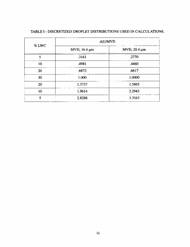
TABLE I - DISCRETIZEDDROPLETDISTRIBUTIONS USED IN CALCULATIONS.

d(I)/MVD% LWC

MVD, 16.4 lam MVD, 20.4 btm

5 .3161 .2770

l0 .4981 .4460

20 .6872 .6617

30 1.000 1.0000

20 1.3737 1.5865

10 1.9614 2.2943

5 2.8288 3.2542

12

SPRAY BAR 1 /

CONTROL ///

ROOM _" PRIMARY /

CONTROL ROOM --/

Figure 1. - NASA Lewis Icing Research Tunnel. Plan view.

MODELACCESS DOOR

CD-95-70602

Figure 2. - Installation of spray system used for Icing Research Tunnel impingement tests.

13

Figure3.- Automatedreflectometerusedtoreduceimpingementdata.

(a)Installationin IRT.

Figure4.- Boeing737-300inlet.

(b) VSAERO panel model.

14

• i

1

I i• t i

(a) Y = 0 plane.

Figure 5. - Boeing 737-300 inlet ICEGRID3D grid model.

Figure 6. - Illustration of inlet blotter strip orientation.

15

.6

.4

.2

.0

e = 0 ° 0 = 45 ° 8 = 90 ° 0 = 135 = 9 = 180 °

7-r p,

(a)W = 7.8 kg/s(z=0 °

.6

n"111rn

.0

Z

I

_C

.4 \_

.2 _.--,--,-_._.

.2

.0

' -",-------+_..___ r" ___ "'_.== __

i' f r r -"

(b)

W = 7.8 kg/sa=15"

(c)W = 10.4 kg/soc=0 °

.6

.4

.2

.0

0 10 20 30 0 10 20 30 0 10

0 10 20 30 0 10 20 30

AXIAL DISTANCE (CM)

20 30

(d)

W = 10.4 kg/sec=15"

THEORY

TEST DATA

Figure 7. - Experimental and analytical surface Mach numbers for the Boeing 737-300 inlet for

airspeed, 75 m/s; static temperature, 7 ° C; static pressure, 95840 Pa.

16

18OO

1200

600

0

O=O ° 0=45" 0=90 ° O= 135 = O= 180 =

i J \

(a)W = 7.8 kg/so[=0 °

0b-I

18OO

1200

600

0

1800

1200

60O

0

j ) I_

A \ .% /m\

(b)W = 7.8 kg/s_=15 °

(c)W = 10.4 kg/s_=0 °

1800

1200

6OO

0

I1

/ J " t \

-21 -7 7 21 -21 -7 7 21 -21 -7 7 21

-21 -7 7 21 -21 -7 7 21

SURFACE DISTANCE FROM HIGHLIGHT (CM)

(POSITIVE VALUES ON INNER SURFACE)

(d)W = 10.4 kg/s_=15"

Figure 8. - Analytical heat transfer distribution for the Boeing 737-300 inlet for airspeed, 75 m/s;

static temperature, 7 ° C; static pressure, 95840 Pa.

17

BETA CONTOURS

_}. qb_:@ :'

11, 7|.10_10

g, 77778

I-1,93333

1 .I]11111

1,08889

1. 16667

1,24444

1,32222

1, ,40000

(a) Monodisperse droplet diameter, 9.08 I.tm. (b) Monodisperse droplet diameter, 66.261/m.

Figure 9. - Analytical collection efficiency for the Boeing 737-300 inlet for angle-of-attack, 0°;

airspeed, 75 m/s; static temperature, 7 ° C; static pressure, 95840 Pa; mass flow, 7.8 kg/s.

BETA CONTOURS

(a) Monodisperse droplet diameter, 20.36 l.tm. (b) Droplet distribution MVD, 20.36 _tm.


airspeed, 75 m/s; static temperature, 7 ° C; static pressure, 95840 Pa; mass flow, 7.8 kg/s.

18

BETA CONTOURS

ii _ 4..i._ i

I!. _.ii_::_.:!

IJ, ?I|[J[]H

i], 77778

ft. 93333

1.01111

I. 08889

1. 16667

1. 24444

1. 32222

1. 40000

(a) Mass flow, 7.8 kg/s. (b) Mass flow, 10.4 kg/s.


airspeed, 75 m/s; static temperature, 7 ° C; static pressure, 95840 Pa; MVD, 20.36 lxm.

BETA CONTOURS

_i i:ii :'

_'_ '::__ ! i_

[], ._;21:f2t!

0, ?lil.][}B

0, ?Z778

8,85556

[I. 93:1::'13

I,gllll

1, I]8889

1,16667

1,24444

1. 32222

1. 40000

(a) Angle-of-attack, 0 °. (b) Angle-of-attack, 15 °.

Figure 12. - Analytical collection efficiency for the Boeing 737-300 inlet for airspeed, 75 m/s;

static temperature, 7 ° C; static pressure, 95840 Pa; MVD, 20.36 I.tm; mass flow, 7.8 kg/s.

19

1.0

>-

ZW

IIt.ItILl

ZoI

I--OILl_.l_JoO

.9

.8

.7

.6

.5

.4

.3

.2

.1

.0

\,\

Repeat 1

..... Repeat 2

Repeat 3

Repeat 4

\

\

i..., LEWICE

-6. -3. .0 3. 6. 9. 12. 15.


Figure 13. - Experimental and analytical collection efficiency for the NACA 65-015 wing for

MVD, 16.45 txrn; angle-of-attack, 8°; airspeed, 75 m/s; static temperature, 7 ° C; static

pressure, 95840 Pa.

1.00

>- 0.83OZILl

0.67ILi.LLw 0.50zoi- 0.330LU.--I

...I0 0.17

0.00

-21.

I

I

I I

THEORY

TEST DATA

0. 7. 14. 21.


(a) Mass flow, 7.8 kg/s; (x, 0°; O = 90 °.

1.00

>-- 0 0.83

zILlI

O 0.67i.g.14.ILlz 0.509I--0 0.33W_1..1

O 0.17O

I I I

THEORY

• TEST DATA -

/J/ -

0.00-21. -14. -7. 0. 7. 14. 21.


(b) Mass flow, 10.4 kg/s; ct, 15°; 0 = 135°.

Figure 14. - Experimental and analytical collection efficiency for the Boeing 737-300 inlet for

MVD, 20.36 _tm; airspeed, 75 m/s; static temperature, 7 ° C; static pressure, 95840 Pa.

20

1.00

.67

.33

.0

9 = 0 ° e = 45 ° 0 = 90" e = 135 ° 9 = 180 °

(a)

W = 7.8 kg/s

MVD = 16.45 I_m

>-0ZILl

L)LLLLLU

ZO

L)LU.J

O(J

1.00

.67

.33

.0

1.00

.67

.33

.0

(b)

W = 7.8 kg/s

MVD = 20.36 I_m

(c)W = 10.4 kg/s

MVD = 16.45 I_m

1.00

.67

.33

.0] J Jt

-21 -7 7 21 -21 -7 7 21 -21 -7 7 21

-21 -7 7 21 -21 -7 7 21



(d)W = 10.4 kg/s

MVD = 20.36 l_m

THEORY

TEST DATA


angle-of-attack, 0°; airspeed, 75 m/s; static temperature, 7 ° C; static pressure, 95840 Pa.

21

e = 0 ° 0 = 45 ° 0 = 90 ° 0 = 135 ° G = 180 °

1.00

.67

.33

.0•1 __. L _7. L

(a)

W = 7.8 kg/sMVD = 16.45 l_m

>.-C)ZW

OLLLLUJ

Zo

roLU_J.JoO

1.00

.67

.33

.0

1.00

.67

.33

.0

7/

f /- /.-_ i. /.7.1 L! J' t ._,' i _..

JL

(b)

W = 7.8 kg/s

MVD = 20.36 l_m

(c)W = 10.4 kg/s

MVD = 16.45 I_m

1.00

.67

.33

.0

-21 -7 7 21 -21 -7 7 21 -21 -7 7 21

-21 -7 7 21 -21 -7 7 21



(d)W = 10.4 kg/s

MVD = 20.36 I_m

THEORY

TEST DATA


angle-of-attack, 15°; airspeed, 75 m/s; static temperature, 7 ° C; static pressure, 95840 Pa.

22

e = 0 ° e = 45" 0 = 90 ° e = 135 ° 0 = 180 °

12

4

-4

O -12

F-"1" 12(.9_J-1- 4(.9

-4

O -12ri-LL

LU 12OZ< 4

-4a

-J -12<a

12n"

-4

-12

-5 3 11 19 -5 3 11 19 -5 3 11 19

-5 3 11 19 -5 3 11 19

AXIAL DISTANCE FROM HIGHLIGHT (CM)

(a)

W = 7.8 kg/s

MVD = 16.45 tim

(b)

W = 7.8 kg/s

MVD = 20.36 I_m

(c)W = 10.4 kg/s

MVD = 16.45 t_m

(d)

W = 10.4 kg/sMVD = 20.36 I_m

Figure 17. - Analytical ice shapes for the Boeing 737-300 inlet for 0 ° angle-of-attack. Icing condi-

tions: airspeed, 75 m/s; icing time, 30 minutes; static temperature, -29.9 ° C; static pres-

sure, 95840 Pa; liquid water content, .2 g/m 3.

23

0=0 ° 0=45 ° 0=90 ° e= 135 ° 0= 180 °

12

4

-4

(3 -12

F-"1- 12(9

-I- 4(9

-4

0 -12n"LL

LU 12L)Z< 4

_-- -4a

-J -12<a<c 12n-

4

-4

-12

Uk_. ....

iP--- IP---- liP'" _ ii,"_--

-5 3 11 19 -5 3 11 19 -5 3 11 19

-5 3 11 19 -5 3 11 19


(a)

W = 7.8 kg/s

MVD = 16.45 I_m

(b)

W = 7.8 kg/s

MVD = 20.36 I_m

(c)W = 10.4 kg/s

MVD = 16.45 l_m

(d)

W = 10.4 kg/s

MVD = 20.36 l_m

Figure 18. - Analytical ice shapes for the Boeing 737-300 inlet for 0° angle-of-attack. Icing condi-

tions: airspeed, 75 m/s; icing time, 30 minutes; static temperature, -9.3* C; static pres-


24

8 = 0 ° e = 45 ° e = 90 ° e = 135 ° 8 = 180 °

12

-4

O_ -12

F-"1- 12(.9..J-r- 4(.9-_ -4

O -12ri-LL

LU 12O

t-- m _-- _ IP_'- le"--

Z

4 ...... _CO 4 _. C C _a

_1 -12<D< 12rr

-4

-12

-5 3 11 19 -5 3 11 19 -5 3 11 19

-5 3 11 19 -5 3 11 19


(a)W = 7.8 kg/sMVD = 16.45 t_m

(b)

W = 7.8 kg/s

MVD = 20.36 I_m

(c)W = 10.4 kg/s

MVD = 16.45 gm

(d)

W = 10.4 kg/sMVD = 20.36 I_m

Figure 19. - Analytical ice shapes for the Boeing 737-300 inlet for 15 ° angle-of-attack. Icing con-

ditions: airspeed, 75 m/s; icing time, 30 minutes; static temperature, -29.9 ° C; static pres-


25

12

-4

(_ -12

I 12i

I 4

_: -4

O -12

II

inn 12OZ

4

CO -4a

-12<a

12

4

-4

O=O" e=45 ° 0=90 ° 0= 135° G= 180°

-12

,,-_ .r .r =t • ir

-5 3 11 19 -5 3 11 19 -5 3 11 19

-5 3 11 19 -5 3 11 19


(a)W = 7.8 kg/sMVD = 16.45 _m

(b)W = 7.8 kg/sMVD = 20.36 _m

(c)W = 10.4 kg/sMVD = 16.45 _m

(d)W = 10.4 kg/sMVD = 20.36 _m

Figure 20. - Analytical ice shapes for the Boeing 737-300 inlet for 15 ° angle-of-attack. Icing con-

ditions: airspeed, 75 m/s; icing time, 30 minutes; static temperature, -9.3* C; static pres-


26

Fon'n ApprovedREPORT DOCUMENTATION PAGE OMBNo. 0704.0100

Public reporting burden for this collection of information is estimated to average 1 hour per response, including the time for reviewing instructions, searching existing data sources,

gathering end maintaining the data needed, and completing and reviewing the collection of information. Send comments regarding this burden estimate or any other aspect of this

collection of information, including suggestions for reducing this burden, to Washington Headquarters Services, Directorate for Information Operations and Reports, 1215 Jefferson

Davis Highway, Suits 1204, Arlington, VA 22202-4302, and to the Office of Management and Budget, Paperwork Reduction Project (0704-0188), Washington, DC 20503.

1. AGENCY USE ONLY (Leave blank) 2. REPORT DATE 3. REPORTTYPE AND DATES COVERED

February 1997 Technical Memorandum

5. FUNDING NUMBERS4. TITLE AND SUBTITLE

Collection Efficiency and Ice Accretion Calculations for a Boeing 737-300 Inlet

6. AUTHOR(S)

Colin S. Bidwell

r. PERFORMING ORGANIZATION NAME(S) AND ADDRESS(ES)



Cleveland, Ohio 44135-3191

9. SPONSORING/MONITORING AGENCY NAME(S) AND ADDRESS(ES)


Washington, D.C. 20546-000 !

WU-505-68-10

8. PERFORMING ORGANIZATION

REPORT NUMBER

E- 10498

10. SPONSORING/MONITORING

AGENCY REPORT NUMBER

NASA TM- 107347

11. SUPPLEMENTARY NOTES

Prepared for the World Aviation Congress cosponsored by the Society of Automotive Engineers and the American

Institute for Aeronautics and Astronautics, Los Angeles, California, October 22-24, 1996. Responsible person, Colin S.

Bidwell, organization code 2720, (216) 433-3947.

12a. DISTRIBUTION/AVAILABILITYSTATEMENT 12b. DISTRIBUTION CODE

Unclassified - Unlimited

Subject Category 02

This publication is available from the NASA Center for AeroSpace Information, (301 ) 621-0390.

13. ABSTRACT (Max/mum 200 words)

Collection efficiency and ice accretion calculations have been made for a Boeing 737-300 inlet using a three-dimensional

panel code, an adaptive grid code, the NASA Lewis LEWlCE3D grid based ice accretion code. Flow solutions for the

inlet were generated using the VSAERO panel code. Grids used in the ice accretion calculations were generated using

the newly developed adaptive grid code ICEGRID3D. The LEWlCE3D grid based ice accretion program was used to

calculate impingement efficiency and ice shapes. Ice shapes typifying rime and mixed icing conditions were generated

for a 30 minute hold condition. All calculations were performed on an SGI Power Challenge computer. The results have

been compared to experimental flow and impingement data. In general, the calculated flow and collection efficiencies

compared well with experiment, and the ice shapes looked reasonable and appeared representative of the rime and mixed

icing conditions for which they were calculated.

14. SUBJECT TERMS

Ice accretion; Inlet icing; Inlet icing prediction; Inlet impingement characteristics; Inlet

collection efficiencies

17. SECURITY CLASSIFICATIONOF REPORT

Unclassified

18. SECURITY CLASSIFICATIONOF THIS PAGE

Unclassified

19. SECURITY CLASSlRCATION

OF ABSTRACT

Unclassified

15. NUMBER OF PAGES28

16. PRICE CODE

A03

20. UMITATION OF ABSTRACT

NSN 7540-01-280-5500 Standard Form 298 (Rev. 2-89)

Prescribed by ANSI Std. Z39-18

298-102

Documents

Collection Efficiency and Ice Accretion Calculations … Efficiency and Ice Accretion Calculations for a Boeing 737-300 Inlet Colin S. Bidwell National Aeronautics and Space Administration