Collegial Activity Learning between Heterogeneous Sensors

Kyle D. Feuz and Diane J. Cook, Fellow, IEEE

Abstract—Activity recognition algorithms have matured and become more ubiquitous in recent years. However, these algorithms

are typically customized for a particular sensor platform. In this paper we introduce PECO, a Personalized activity ECOsystem,

that transfers learned activity information seamlessly between sensor platforms in real time so that any available sensor can

continue to track activities without requiring its own extensive labeled training data. We introduce a multi-view transfer learning

algorithm that facilitates this information handoff between sensor platforms and provide theoretical performance bounds for the

algorithm. In addition, we empirically evaluate PECO using datasets that utilize heterogeneous sensor platforms to perform activity

recognition. These results indicate that not only can activity recognition algorithms transfer important information to new sensor

platforms, but any number of platforms can work together as colleagues to boost performance.

Index Terms—activity recognition, machine learning, transfer learning, pervasive computing

—————————— ——————————

1 INTRODUCTION

CTIVITY recognition and monitoring lie at the center of

many fields of study. An individual’s activities affect that

individual, the people nearby, society, and the environment.

In the past, theories about behavior and activity were formed

based on self-report and limited in-person observations. More

recently, the maturing of sensors, wireless networks, and

machine learning have made it possibly to automatically learn

and recognize activities from sensor data. Now, activity

recognition is becoming an integral component of

technologies for health care, security surveillance, and other

pervasive computing applications.

As the number and diversity of sensing devices increase, a

personalized activity monitoring ecosystem can emerge.

Instead of activity recognition being confined to a single

setting, any available device can “pick up the gauntlet” and

provide both activity monitoring and activity-aware services.

The sensors in a person’s home, phone, vehicle, and office can

work individually or in combination to provide robust activity

models.

One challenge we face in trying to create such a

personalized ecosystem is that training data must be available

for each activity based on each sensor platform. Gathering a

sufficient amount of labeled training data is labor-intensive for

the user.

Transfer learning techniques have been proposed to handle

these types of situations where training data is not available

for a particular setting. Transfer learning algorithms apply

knowledge learned from one problem domain, the source, to

a new but related problem, the target (see Fig. 1). While these

algorithms typically rely on shared feature spaces or other

common links between the problems, in this paper we focus

on the ability to transfer knowledge between heterogeneous

activity learning systems where the domains, the tasks, the

data distributions, and even the feature spaces can all differ

between the source and the target.

As an example, consider a scenario where training data

was provided to train a smart home to recognize activities

based on motion and door sensors. If the user wants to start

using a phone-based recognizer, the label-and-train process

must be repeated. To avoid this step, we design an omni-

directional transfer learning approach, or collegial learning,

that allows the smart home to act as a teacher to the phone and

allows the phone in turn to boost the performance of the smart

home’s model. In this paper, we describe collegial activity

learning and its implementation in the PECO system. We

derive expected upper and lower performance bounds and

empirically analyze the approach using ambient, wearable,

phone, and depth camera sensor data.

2 ACTIVITY RECOGNITION

Our proposed Personalized activity ECOsystem, PECO,

builds on the notion of activity recognition, or labeling

activities based on a sensor-based perception of the user and

xxxx-xxxx/0x/$xx.00 © 200x IEEE Published by the IEEE Computer Society

————————————————

Kyle D. Feuz is with the Department of Computer Science, Weber State University, Ogden, UT 84408. E-mail: kylefeuz@weber.edu.

Diane J. Cook is with the School of Electrical Engineering and Computer Science, Washington State University, Pullman, WA 99164. E-mail: cook@eecs.wsu.edu.

A

Fig. 1. In traditional machine learning, training and testing data come from the same domain and have similar distributions. In contrast, transfer learning uses knowledge from a different, related domain to improve learning for a new domain. In a personalized activity ecosystem, the home, phone, wearable, and camera use transfer learning to act as colleagues despite their diversity.

2 IEEE TRANSACTIONS ON PATTERN ANALYSIS AND MACHINE INTELLIGENCE

the environment. Let e represent a sensor reading and x be a

sequence of such sensor readings, e1,… en. Y is a set of

possible activity labels and y is the activity label associated

with a particular sequence of sensor events such as x. The

problem of activity recognition is to map features describing

a sequence of sensor readings (sensor events), x=<e1 e2 …

en>, onto a value from a set of predefined activity labels,

yY. This is typically accomplished by using a supervised

machine learning algorithm that learns the mapping based on

a set of sample data points in which the correct label is

provided.

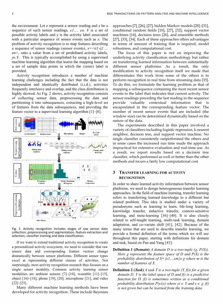
Activity recognition introduces a number of machine

learning challenges including the fact that the data is not

independent and identically distributed (i.i.d.), activities

frequently interleave and overlap, and the class distribution is

highly skewed. As Fig. 2 shows, activity recognition consists

of collecting sensor data, preprocessing the data and

partitioning it into subsequences, extracting a high-level set

of features from the data subsequences, and providing the

feature vector to a supervised learning algorithm [1]–[6].

If we want to extend traditional activity recognition to create

a personalized activity ecosystem, we need to consider that raw

sensor data and corresponding feature vectors change

dramatically between sensor platforms. Different sensor types

excel at representing different classes of activities. Not

surprisingly, most activity recognition research thus focuses on a

single sensor modality. Common activity learning sensor

modalities are ambient sensors [7]–[10], wearable [11]–[15],

object [16]–[18], phone [19], [20], microphone [21], and video

[22]–[25].

Many different machine learning methods have been developed for activity recognition. These include Bayesian

approaches [7], [26], [27], hidden Markov models [28]–[31], conditional random fields [10], [27], [32], support vector machines [14], decision trees [26], and ensemble methods [27], [33], [34]. Each of these approaches offers advantages in terms of amount of training that is required, model robustness, and computational cost.

The focus of this paper is not on improving the underlying activity classification methodology but rather on transferring learned information between substantially different sensor platforms. As a result, the only modification to activity recognition itself we made that differentiates this work from some of the others is to perform recognition in real time from streaming data [35]. To do this, we formulate the learning problem as that of mapping a subsequence containing the most recent sensor events to the label that indicates that current activity. The sensor readings preceding the last reading in the sequence provide valuable contextual information that is encapsulated in the corresponding feature vector. The number of recent sensor events that are included (the window size) can be determined dynamically based on the nature of the data.

The experiments described in this paper involved a variety of classifiers including logistic regression, k nearest neighbor, decision tree, and support vector machine. No single classifier consistently outperformed the others and in some cases the increased run time made the approach impractical for extensive evaluation and real-time use. As a result, we report results based on a decision tree classifier, which performed as well or better than the other methods and incurs a fairly low computational cost.

3 TRANSFER LEARNING FOR ACTIVITY

RECOGNITION

In order to share learned activity information between sensor

platforms, we need to design heterogeneous transfer learning

approaches. In the field of machine learning, transfer learning

refers to transferring learned knowledge to a different but

related problem. This idea is studied under a variety of

pseudonyms such as learning to learn, life-long learning,

knowledge transfer, inductive transfer, context-sensitive

learning, and meta-learning [36]–[40]. It is also closely

related to self-taught learning, multi-task learning, domain

adaptation, and co-variate shift [41], [42]. Because of the

many terms that are used to describe transfer learning, we

provide a formal definition of the terms which we will use

throughout this paper, starting with definitions for domain

and task, based on Pan and Yang [43]:

Definition 1 (Domain) A domain D is a two-tuple (, P(X)).

Here represents the feature space of D and P(X) is the

probability distribution of X={x1,..,xm} where m is the

number of features of X.

Definition 2 (Task) A task T is a two-tuple (Y, f()) for a given

domain D. Y is the label space of D and f() is a predictive

function for D. f() is sometimes written as a conditional

probability distribution P(yi|x) where yi Y and x . f()

is not given but can be learned from the training data.

Fig. 2. Activity recognition includes stages of raw sensor data collection, preprocessing and segmentation, feature extraction and selection, classifier training and data classification.

FEUZ ET AL: COLLEGIAL ACTIVITY LEARNING BETWEEN HETEROGENEOUS SENSORS 3

In the case of activity recognition, the domain is defined

by the feature space based on the most recent sensor readings

and a probability distribution over all possible feature values.

In the activity recognition example given earlier the set of

sensor readings x is one instance of x . The task is

composed of a label space Y which contains the set of labels

for activities of interest together with a conditional

probability distribution representing the probability of

assigning label yiY given the observed data point x. We

can then provide a definition of transfer learning.

Definition 3 (Transfer Learning) Given a set of source domains

DS = {Ds1, .., Dsn}, n>0, a target domain Dt, a set of source

tasks TS = {Ts1, .., Tsn} where TsiTS corresponds with

DsiDS, and a target task Tt which corresponds with Dt,

transfer learning improves the learning of the target

predictive function f() in Dt, where DtDS and/or TtTS.

Definition 3 encompasses many transfer learning

scenarios. The source domains can differ from the target by

having a different feature space, a different distribution of

data points, or both. The source tasks can also differ from the

target task by having a different label space, a different

predictive function, or both. In addition, the source data can

differ from the target data by having a different domain, a

different task, or both. However, all transfer learning

problems rely on the assumption that there exists some

relationship between the source and target which allows for

successful transfer of knowledge from source to target.

Previous work on transfer learning for activity recognition

has focused primarily on transfer between users, activities, or

settings. While most of these methods are constrained to one

set of sensors [44]–[50], a few efforts have focused on

transfer between sensor types. In addition to the teacher-

learner model we will discuss later [51], Hu and Yang [52]

introduced a between-modality transfer technique that

requires externally-provided information about the

relationship between the source and domain spaces.

Other transfer learning approaches have been developed

outside activity learning that can be valuable for sharing

information between heterogeneous sensor platforms. For

example, domain adaptation allows different source and

target domains, although typically the only difference is in the

data distributions [53]. Differences in data distributions have

been considered when the source and target domain feature

spaces are identical, using explicit alignment techniques

[54]–[56]. In contrast, we focus on transfer learning problems

where the source and target domains have different feature

spaces. This is commonly referred to as heterogeneous

transfer learning, defined below.

Definition 4 (Heterogeneous Transfer Learning) Given

domains DS, domain Dt, tasks TS, and task Tt as defined in

Definition 3, heterogeneous transfer learning improves the

learning of the target predictive function ft() in Dt, where

t (s1..sn)=.

Heterogeneous transfer learning methods have not been

attempted for activity recognition, although they have been

explored for other applications. Some previous research has

yielded feature space translators [57], [58] as well as

approaches in which both feature spaces are mapped to a

common lower-dimensional space [59], [60]. Additionally,

previous multi-view techniques utilize co-occurrence data, or

data points that are represented in both source and target

feature spaces [61]–[63].

There remain many open challenges in transfer learning.

One such challenge is performing transfer-based activity

recognition when the source data is not labeled. Researchers

have leveraged unlabeled source data to improve transfer to

the target domain [41], [64], but such techniques have not

been applied to activity recognition nor used in the context of

multiple source/target differences. We address both of these

challenges in this paper by introducing techniques for

transferring knowledge between heterogeneous feature

spaces, with or without labeled data in the target domain.

Note that this work differs from multi-sensor fusion for

activity learning [65]–[67]. Sensor fusion techniques combine

data derived from diverse sensory data. However, they

typically require that training data be available for all of the

sensor types. In contrast, we are interested in providing a

“cold start” for new sensor platforms that allow them to

perform activity recognition with minimal training data of

their own. The unique contributions of this work thus center

on both two new approaches to multi-view learning with

theoretical bounds and on development of a real-time

personalized ecosystem that transfers activity knowledge in

real time between heterogeneous sensor platforms.

Co-Training methods have been available for years as a semi-

supervised machine learning technique, but have rarely if ever

been applied as a transfer learning technique between

heterogeneous systems. Furthermore, extending them to work

without labeled data in the target learning space is critical to

deploying new learning systems with minimal user-effort

required. Lastly, the learning bounds are useful both from a

theoretical viewpoint and also from a practical viewpoint.

Previously, predicting the accuracy of a learning system required

labeled data in the target space, but now we can both train a

learning system and predict its accuracy without requiring any

user-labeled data in the target domain.

4 PERSONALIZED ECOSYSTEM

Every day brings new advances in sensing and data

processing. Given the increasing prevalence of diverse

sensors, we need to be able to introduce new activity sensory

devices without requiring additional training time and effort.

In response, we are designing multi-view techniques to

transfer knowledge between activity recognition systems. The

goal is to increase the accuracy of the collaborative ecosystem

while decreasing the need for new labeled data.

To illustrate our approach, recall the earlier example in

which a home (source view) is equipped with ambient sensors

to monitor motion, lighting, temperature, and door use. The

resident now wants to train smart phone sensors (target view)

to recognize the same activities. Whenever the phone is

located inside the home, both sensing platforms collect data

while activities are performed, resulting in a multi-view

learning opportunity where the ambient sensors represent one

view and the phone sensors represent a second view. If the

phone can be trained, it can also monitor activities outside of

the home and can update the home’s model when the resident

4 IEEE TRANSACTIONS ON PATTERN ANALYSIS AND MACHINE INTELLIGENCE

returns. The phone may converge upon a stronger model than

the home either because it receives training data of its own or

because it has a more expressive feature space. In these cases,

the target view can be used to actually improve the source’s

model. We will consider both informed and uninformed

approaches to multi-view learning, distinguished by whether

labeled data is available in the target domain (informed) or

not (uninformed).

4.1 Informed Multi-View Learning

Two techniques have been extensively used by the

community for multi-view learning when labeled training data

is available in the target domain. In Co-Training [62], a small

amount of labeled data in each view is used to train a separate

classifier for each view (for example, one for the home and one

for the phone). Each classifier then assigns labels to a subset of

the unlabeled data, which can be used to supplement the

training data for both views. We first adapt Co-Training for

activity recognition, as summarized in Algorithm 1. While

Algorithm 1 is designed for binary classification, it can handle

activity recognition with more than two classes by allowing

each view to label positive examples for each activity class.

Algorithm 1: Co-Training

Input: a set L of labeled activity data points

a set U of unlabeled activity data points

Create set U’ of u examples, U’ U

while U’ ≠ do

Use L to train activity recognizer h1 for view 1

…

Use L to train activity recognizer hk for view k

Label most confident p positive data points and

n negative data points from U’ using h1

…

Label most confident p positive data points and

n negative data points from U’ using hk

Add the newly-labeled data points to L

Add k(p + n) data points from U to U’

Algorithm 2: Co-EM

Input: a set L of labeled activity data points

a set U of unlabeled activity data points

Use L to train classifier h1 on view 1

Create set U1 by using h1 to label U

for i = 0 to m do

Use L U1 to train classifier h2 on view 2

Create set U2 by using h2 to label U

…

Use L Uk-1 to train classifier hk on view k

Create set U1 by using hk to label U

The second informed technique, Co-EM, is a variant of Co-

Training that has been shown to perform better in some

situations [68]. Unlike Co-Training, Co-EM labels the entire

set of unlabeled data points every iteration. Training continues

until convergence is reached (measured as the number of labels

that change each iteration) or a fixed number of iterations m is

performed, as in Algorithm 2. We can introduce additional

classifiers as needed, one for each view. Each view can also

employ a different type of classifier, as is best suited for the

corresponding feature space.

4.2 Uninformed Multi-View Learning

In a personalized ecosystem, labeled data is not always

available in the target domain. This would happen, for example,

when a new sensor platform is first integrated into the

ecosystem. In this situation, we need to use an uninformed

multi-view technique. Uninformed multi-view algorithms have

been proposed and tested for applications such as text mining

[69]. One such algorithm is Manifold Alignment [70], which

assumes that the data from both views share a common latent

manifold which exists in a lower-dimensional subspace. If this

is true, then the two feature spaces can be projected onto a

common lower-dimensional subspace using Principal

Component Analysis [71]. The subsequent pairing between

views can be used to optimally align the subspace projections

onto the latent manifold using a technique such as Procrustes

analysis. A classifier can then be trained using projected data

from the source view and tested on projected data from the

target view. This is summarized in Algorithm 3.

Algorithm 3: Manifold Alignment Algorithm (two views)

Input: a set L of labeled activity data points in view 1

sets U1, U2 of paired unlabeled data points

(one set for each view)

X,EV1 = PCA(U1) // map U1 onto lower-dimensional space

Y = PCA(U2) // map U2 onto same space

// Apply Procrustes Analysis to align X and Y

UVT SVD(YTX)

Q U VT

k Trace() / Trace(YTY)

Y’ kYQ

Project L onto low-dimensional embedding using EV

Train classifier on projected L

Test classifier on Y’

Finally, we consider a teacher-learner model that was

introduced by Kurz et al. [51] to train new views that have no

labeled training data. This approached, summarized in

Algorithm 4, can be applied in settings where labeled activity

data is available in the source view but not the target view.

We note that the teacher-learner algorithm is equivalent to a

single-iteration version of Co-EM when no labeled data is

available in the target view. This observation allows us to

provide a theoretical foundation for the technique. Valiant [72]

introduced the notion of Probably Approximately Correct

(PAC) learning to determine the probability that a selected

classification function will yield a low generalization error.

Blum and Mitchell [62] show that multi-view learning has PAC

bounds when three assumptions hold: 1) the two views are

conditionally independent given the class label, 2) either view

is sufficient to correctly classify the data points, and 3) the

accuracy of the first view is at least weakly useful.

In this paper, we enhance these baseline multi-view learning

approaches for application to activity learning, specifically for

multiple activity classes. We also introduce new approaches to

FEUZ ET AL: COLLEGIAL ACTIVITY LEARNING BETWEEN HETEROGENEOUS SENSORS 5

multi-view learning for this problem and provide a PAC

analysis for the proposed PECO approach.

Algorithm 4: Teacher-Learner Algorithm

Input: a set L of labeled activity data points in view 1

a set U of unlabeled data points

Use L to train activity recognizer h1 for view 1

Create set U1 by using h1 to label U

Use U1 to train classifier h2 on view 2

…

Use U1 to train classifier hk on view k

Algorithm 5: PECO Algorithm

Input: a set L of labeled activity data points in view 1

a set U of unlabeled data points

Use L to train activity recognizer h1 for view 1

Create set U1 by using h1 to label U’ U

L = L U1

U = U - U1

Apply Co-Training or Co-EM

4.3 Personalized ECOsystem (PECO) Algorithm

Our PECO (Personalized ECOsystem) approach to multi-

view learning combines the benefits of iterative informed

strategies such as Co-Training and Co-EM with the benefits of

using teacher-provided labels for new uninformed sensor

platforms that have no labeled activity data for training. The

PECO approach is summarized in Algorithm 5. Not only can

PECO facilitate activity recognition in a new view with no

labeled data, but in some cases the accuracy of view 1 actually

improves when view 2, the target view, subsequently takes on

the role of teacher and updates view 1’s model. This illustrates

our notion of collegial learning.

In the PECO algorithm, the teacher (source view, view 1)

initially provides labels for a few data points that both the

teacher and the learner (target view, view 2) observe with their

different sensors and represent with their different feature

vectors. Next, PECO transitions to an iterative strategy by

applying Co-Training or Co-EM. In this way, the learner can

continue to benefit from the teacher’s expertise while at the

same time contributing its own knowledge back to the teacher,

as a colleague.

In our home-phone transfer scenario, the smart home may

initially act as a teacher because it has labeled activity data

available and the phone does not. When the home and phone

are co-located, the home can opportunistically “call out”

activity labels that the phone can use to label the data captured

in its own sensor space. Eventually the resident may grab their

phone and leave the home. While out, the phone will observe

new activity situations and may even receive labels from the

user for those situations. When the individual returns home, the

home and phone act as colleagues, transferring expertise from

each independent classifier and feature representation to

improve the robustness of both activity models for both sensor

platforms. This scenario can be extended for any number of

types and diversity of sensor platforms, thus airport cameras

can receive information from an individual’s smart phone to

improve activity recognition for security purposes and vehicle

can learn an individual’s activity patterns to help keep drivers

and passengers safe.

In addition to the new PECO algorithm, we introduce a

second multi-view approach that handles more than two views,

which we refer to as Personalized ECOsystem with Ensembles,

or PECO-E. PECO-E first combines multiple teacher views

into a single view using a weighted voting ensemble where

each vote is weighted by the classifier’s confidence in the

activity label. This newly-formed teacher model can then

transfer its knowledge to the learner view using one of the

existing binary multi-view techniques described in Sections 4.2

and 4.3.

4.4 Online Transfer Learning

In order to demonstrate the ability to transfer activity

knowledge between sensor platforms in real time, we

implemented PECO as part of the CASAS smart home system

[73]. The CASAS software architecture is shown in Fig. 3. The

CASAS physical layer includes sensors and actuators. The

middleware layer is driven by a publish/subscribe manager

with named broadcast channels that allow bridges to publish

and receive text messages. The middleware also provides

services such as adding time stamps to sensor readings,

assigning unique identifiers to devices, and maintaining the

state of the system. Every CASAS component communicates

via a customized XMPP bridge to this manager. These bridges

include the Zigbee bridge to provide network services, the

Scribe bridge to archive data, and bridges for each of the

software components in the application layer including PECO.

When the sensors generate readings they are sent as text

messages to the CASAS middleware. PECO’s activity

recognition algorithm generates activity labels for sensor

readings in real time as they are received from one sensor

platform. A new sensor platform can be announced to CASAS

and integrated without any other changes to the system, simply

by announcing its presence and function. Activity labels can

then be sent from the middleware to PECO’s new sensor view

Fig. 3. CASAS software architecture to support real-time transfer learning between heterogeneous platforms.

6 IEEE TRANSACTIONS ON PATTERN ANALYSIS AND MACHINE INTELLIGENCE

in real time in order to bring the new sensor platform up to

speed.

Implementing a personalized ecosystem within CASAS

provides the ability to seamlessly introduce new sensor

capabilities and transfer knowledge from one platform to

another and back. Transferring this information will typically

boost the activity recognition performance for both platforms.

The actual benefit of this transfer, however, is dependent upon

factors such as the strength of the original activity recognition

algorithms and the amount of agreement between the

algorithms. In the next section, we derive theoretical bounds on

expected performance based on these parameters.

4.5 PECO Accuracy Bounds

Without labeled activity data in the target view, we cannot

compute performance measures such as model accuracy. We

can, however, still derive theoretical bounds for worst-case,

best-case, and expected-case learner performance. We make

the assumption that the previously-observed teacher accuracy

on labeled data is a good indicator of the teacher’s accuracy on

unlabeled data. Our accuracy bound also relies on the average

level of agreement, q, between the teacher and learner for

unlabeled data points in U. We define q in Equation 1, where

h1(x) is the teacher’s activity label for data point x and h2(x) is

the learner’s label for x.

UxUq

(x)h(x)hif0

(x)h(x)hif1

||

1

21

21

(1)

In the case of binary classification tasks, Equation 2

calculates the expected accuracy of the learner, r. This

calculation assumes that the teacher-learner agreement is

independent of the teacher’s classification accuracy, p.

(2)

The first term, pq, represents the expected accuracy of the

learner given that the teacher correctly classifies the data point.

The second term represents the expected learner accuracy

given that the teacher incorrectly classifies the data point. Note

that the learner can only be accurate in the second case when it

disagrees with the teacher.

To generate upper and lower learner accuracy bounds, we

must consider both teacher-learner agreement when the teacher

is correct (q1) and the agreement when the teacher is incorrect

(q2). Substituting these variables into Equation 2 results in

Equation 3. Accuracy is then optimized by maximizing q1 and

minimizing q2.

)1)(1(* 21 qpqpr (3)

Here q1 and q2 are subject to the following constraints:

,*)1(* 21 qqpqp

and,10 1 q

.10 2 q

These constraints ensure that the original level of agreement

q is preserved and that q1 and q2 are valid levels of agreement.

Note that in the first constraint, minimizing q2 maximizes q1

and vice versa. If p ≥ q then q2 has a minimum value of 0 and

all the constraints are satisfied. This implies that q1=q/p is the

maximum value of q1. Substituting this expression into

Equation 3 results in Equation 4.

pqr 1 (4)

If p < q then q1 has a maximal value of 1 and all of the

constraints are satisfied. This implies that q2 = (q-p)/(1-p) is the

minimum value of q2. Substituting into Equation 3 results in

Equation 5.

qpr 1 (5)

Equations 4 and 5 can then be combined into Equation 6,

which represents the upper bound on learner accuracy.

qpr 1 (6)

Next, the lower bound on learner accuracy can be derived

by minimizing q1 and maximizing q2 in Equation 3, subject to

the same constraints on q1 and q2. If (1-p) ≥ q then q1 has a

minimum value of 0 and all the constraints are satisfied. This

implies that q2 = q/(1-p) is the maximum value of q2.

Substituting into Equation 3 results in Equation 7.

qpr 1 (7)

If (1-p) < q then q2 has a maximum value of 1 and all of the

constraints are satisfied. This implies that q1 = (q-1+p)/p is the

minimum value of q1. Substituting in Equation 3 results in

Equation 8.

pqr 1 (8)

Finally, Equations 7 and 8 are combined into Equation 9,

which calculates the lower bound on learner accuracy.

qpr 1 (9)

We can now extend these bounds for the k-ary classification

problem. We first note that we can add an additional term, z, to

Equation 2 which represents the probability that the learner

correctly classifies a data point given that the teacher

misclassified it and the teacher and learner disagree. The result

is shown in Equation 10.

zqppqr )1)(1( (10)

In binary classification, z=1 and can be ignored. Similarly,

the upper bound for k-ary classification will also have z=1 so

our upper bound does not change. The lower bound for k-ary

classification will have z=0 which leads to a lower bound of 0

if (1-p) ≥ q. If (1-p) < q then the lower bound does not change

from Equation 9. For the expected bounds, in the k-ary case, z

≤ 1. We propose two estimates for z. The first estimate

considers the number of classes but not the distribution of the

classes, z = 1/(k-1). The second estimate factors in the

distribution of class labels and is shown in Equation 11. In this

equation, P(y) represents the probability that a data point has a

label of y, where yY. P(y) can be estimated using the observed

frequency of each class.

(11)

Intuitively, z represents the product of the probability that

)1(2

)1)(1(

pqpq

qppqr

Yx YxyyP

xP

xP 2

2)(

))(1(

)(

Yx Yxy xPxP

yPyPxPz

))(1))((1(

)()()(

FEUZ ET AL: COLLEGIAL ACTIVITY LEARNING BETWEEN HETEROGENEOUS SENSORS 7

the teacher assigns a class label of x, the probability that y is the

true class label, and the probability that the learner selects the

correct class label of y, the result of which is summed over each

possible class value and is normalized by the remaining

probabilities given that x is not the class label.

Note that the above analysis assumes that teacher-learner

agreement is uniform over all classes. We can extend this

analysis to consider = P(h1()=x|f1()=y), the probability that

the teacher classifies a data point as x given that it has a true

label of y. Similarly, we consider = P(h2()=y|h1()=y), the

probability that the learner classifies the data point as y given

that the teacher classified it as x. Both of these probabilities can

be estimated without using any labeled data in the learner view.

The expected bound is then calculated in Equation 12. In this

case, we no longer explicitly distinguish between the teacher

being right and wrong. Instead, these cases are handled

implicitly by y=x and yx.

Yy YxyPr )( (12)

In addition to these upper and lower bound learner accuracy

estimates, we can also estimate average performance. A simple

estimation can be performed by averaging upper and lower

bounds, which avoids calculating class distributions and

conditional probabilities. This also avoids making explicit

assumptions about the probability of the teacher and learner

agreeing. Interestingly, when p≥q and (1-p)<q then the average

of the upper and lower bounds is just q.

Note that the expected accuracy of the learner can be

simplified to the underestimate of r=pq. All of the above

bounds provide insight on the expected learner performance

based on characteristics of the teacher, without requiring

labeled data in the learner view. To compute these bounds in

practice, teacher accuracy can be estimated using its labeled

data. Similarly, teacher-learner agreement can be estimated

using unlabeled data in both views. Later, we empirically

compute performance and compare it with these theoretical

bounds.

5 EXPERIMENTAL EVALUATION

The goal of PECO is to transfer activity knowledge from one

sensor platform’s trained view to another sensor platform’s

untrained view. Here we evaluate whether a new sensor

platform can learn these activity models without having any

labeled activity data in its own view. We observe influence

based on the choice of teacher view and consider more than two

views in combination. In addition, we compare theoretical

bounds with observed performance. Finally, we observe the

beneficial effects to the teacher from the transfer, which allows

sensor platforms to act as colleagues.

For our experiments, we make use of three activity

recognition datasets. All of these contain data from multiple

heterogeneous sensor types and all include data from multiple

participants. In each experiment, we report results using 10-

fold cross validation averaged over all participants.

In the Opportunity dataset [74], 4 participants perform 5

repetitions of the following scripted activities: groom, relax,

make/drink coffee, make/drink sandwich, clean, and execute

a simple-movement drill. Twelve 3-axis wearable

accelerometers represent one sensor platform (view 1) and

seven wearable inertial measurement units represent the

second platform (view 2). We use the same features as Sagha

et al. [75] which consist of raw sensor values sampled every

500ms and averaged over a 5-second window.

In the CASAS PUCK dataset [76] (ailab.wsu.edu/casas/

datasets.html), 10 participants perform 3 repetitions of 6

scripted activities: sweep, take medicine, cook oatmeal, water

plants, wash hands, and clean countertops. Activities are

performed in a smart home that is equipped with infrared

motion sensors and magnetic door sensors (view 1). Each

Fig 4. Feature space sizes (top) and data point distribution for the Opportunity (second), PUCK (third), and Parkinson’s (bottom) datasets.

8 IEEE TRANSACTIONS ON PATTERN ANALYSIS AND MACHINE INTELLIGENCE

participant wears two 6-axis accelerometers (view 2). Finally,

object vibration sensors (view 3) are attached to the broom,

dustpan, duster, pitcher, bowl, measuring cup, glass, fork,

watering can, hand soap dispenser, dish soap dispenser,

medicine dispenser, and medicine bottles. For consistency, we

employ the same wearable sensor features as in the

Opportunity dataset. For views 1 and 3, the feature vector

consists of the number of activations for each sensor during

the sampling period.

In the CASAS Parkinson’s dataset, 6 participants perform

3 repetitions of the same activities as in the PUCK dataset. In

addition to the ambient sensor view (view 1), wearable

accelerometer view (view 2), and object sensor view (view

3), a new view is introduced corresponding to Kinect depth

cameras (view 4) that were placed in the smart home.

All of the existing and new algorithms described in this

paper can partner with virtually any classifier. We

experimented with logistic regression, k nearest neighbors,

support vector machines, and decision trees. No classifier

consistently performed best or significantly outperformed the

others on average. We report all of our results here based on

a decision tree classifier, which performed as well or better

than other approaches on average. We utilize a Kinect API

that processes the video data into the 20 (x,y,z) joint positions

found in the video.

Fig. 4 summarizes the size of each view’s feature space

and the distribution of data points across activities for each

dataset. Fig. 5 provides a floor plan and sensor layout for the

PUCK and Parkinson’s datasets, and Figs. 6 and 7 illustrate

the sensor types and locations used in these datasets.

We are ultimately interested in seeing if one sensor platform

can successfully transfer activity knowledge to a new platform.

Fig 6. Motion (top) and object (bottom) sensors in the home.

Fig 5. Smart home floor plan with placement of sensors for motion (M,MA), door (D), temperature (T), object (I), and Kinect (K).

Fig. 8. Accuracy and recall scores for each sensor view using all of the labeled data for the PUCK data.

K01

K03

K02

Fig 7. Placement of wearable accelerometers.

FEUZ ET AL: COLLEGIAL ACTIVITY LEARNING BETWEEN HETEROGENEOUS SENSORS 9

First, we consider the baseline performance of each sensor

view without transfer learning. Fig. 8 plots the performance of

the sensor views in decrasing order of recognition performance

when the view has all of the available labeled data for training

and testing. As we can see, performance varies between the

platforms. The varied strengths of each view will be utilized in

later experiments when we analyze effects of the choice of

teacher views on performance. For each experiment, we

measure performance as activity classification accuracy (see

Equation 13). Because the datasets exhibit a skewed class

distribution (see Fig. 4), for some experiments we also report

average recall scores (see Equation 14). In both of these

equations N is the total number of instances, K is the number

of labels, and A is the confusion matrix where Aij is the number

of instances of class i classified as class j.

𝐴𝑐𝑐𝑢𝑟𝑎𝑐𝑦 = 1

𝑁∑ 𝐴𝑖𝑖

𝐾𝑖=1 (13)

𝐴𝑣𝑔. 𝑅𝑒𝑐𝑎𝑙𝑙 = 1

𝐾∑ 𝐴𝑖𝑖 ∑ 𝐴𝑖𝑗

𝐾𝑗=1

𝐾𝑖=1 (14)

5.1 Informed Learning with Two Views

We initially consider scenarios in which two sensor

platforms are used. With informed methods, both platforms

have a limited amount of training data and act as colleagues to

boost each other’s performance based on the different

perspectives of the data. For each of the 10 cross-validation

folds, the dataset D is split into three pieces: a labeled subset,

an unlabeled subset and a validation subset. The size of the

validation subset is always |D|/10. We then vary the size of the

labeled subset to show how each algorithm performs with

different amount of labeled data. To see how the informed

multiview learning algorithms perform in this scenario, we plot

classification accuracy as a function of the fraction of the

available training data that is provided to both views. We

evaluate these algorithms on the Opportunity and PUCK

datasets.

In order to provide a basis for comparison, we provide three

different baseline approaches. The first baseline, Oracle, uses

an expert (the ground truth labels) to provide the correct labels

for the unlabeled data. The second baseline, None, trains a

classifier using only the target’s labeled subset. The third

baseline, Random, randomly assigns an activity label weighted

by the class distribution observed in the labeled subset. For the

Opportunity dataset, we specify (p=10) examples to label for

the Co-Training algorithm and (m=3) iterations for Co-EM. For

the PUCK dataset, we specify (p=10) for Co-Training and

(m=10) for Co-EM. We experimented with alternative values

for both datasets and algorithms but observed little variation in

the resulting accuracies. Fig. 9 plots the resulting accuracies

and Fig. 10 plots the average recall scores. As expected, the multiview algorithms start at the same

accuracy as Random but converge near the same accuracy as

Oracle as the amount of labeled data in each view increases.

The effect of transfer learning can be seen when comparing the

CoTrain and CoEM curves with the None baseline. The results

are mixed (differences between approaches are significant as

determined by a one-way ANOVA, p<0.05). In the PUCK

dataset only Co-EM outperforms None, and in the Opportunity

dataset None outperforms both approaches. This may be due to

the fact that the two views not only violate the conditional

independence assumption but in the case of the Opportunity

dataset the sensors are quite similar and are therefore highly

correlated. 5.2 Uninformed Learning with Two Views

We next repeat the previous experiment using uninformed

techniques. This means that the labeled data is only available

to the source view. A second sensor platform is later brought

online (the target view) but has no training data and is therefore

completely reliant on transferred information from the source.

For both the PUCK and Opportunity datasets, we select d for

the Manifold Alignment algorithm to be set to the minimum

number of dimensions found in the source and target views,

which therefore maximizes the information that is retained by

the dimensionality reduction step. Figs. 11 and 12 show the

results. Again, a one-way ANOVA indicates that the differences

between the means of the techniques are significant, p<0.05.

Fig. 9. Classification accuracy of informed multiview approaches for the PUCK (top) and Opportunity (bottom) datasets as a function of the fraction of training data that is used by both target and source views (on a log scale).

Fig. 10. Average recall of informed multiview approaches for the PUCK (left) and Opportunity (right) datasets as a function of the fraction of training data that is used, on a log scale.

10 IEEE TRANSACTIONS ON PATTERN ANALYSIS AND MACHINE INTELLIGENCE

As shown in these graphs, Manifold Alignment does not

perform well, although it does improve as more data becomes

available in the Opportunity dataset. This is likely due to the

invalid assumption that data from both source and target views

can be projected onto a shared manifold in a lower-dimensional

space. This is particularly problematic for the PUCK dataset

because the sensor platforms are very different. In contrast, the

Teacher-Learner method does clearly improve as the amount of

labeled source data increases. In fact, it approaches the ideal

accuracy achieved by the Oracle baseline.

This leads us to the evaluation of our PECO algorithm on

the PUCK dataset. In this case we divide the original data into

four parts: A labeled subset, a bootstrap subset, an unlabeled

subset and a validation subset. As before, the validation subset

size is |D|/10. The labeled subset is 40% of the remaining data.

The bootstrap subset size varies and the unlabeled subset

contains the remaining data. Only the source view (view 1) is

trained on the labeled data. After training, the source view acts

like a teacher and bootstraps the target view (view 2) by

labeling the bootstrapped portion of the data. The target view

then uses this bootstrapped data to create an initial model. Now

PECO can employ an informed technique like Co-Training or

Co-EM to refine the model. This simulates the situation in

which a well-trained activity recognition algorithm is in place

for one sensor platform, and we introduce a second sensor

platform without providing it any labeled data. We train it using

the source view and subsequently allow both views to improve

each other’s models.

Fig. 13 shows the results of this experiment as a function of

the amount of labeled data in the source view. In this and the

remaining experiments, the weighted recall results are very

similar to the accuracy results so these graphs are omitted. As

shown here, PECO outperforms Teacher-Learner when using

Co-EM. The performance in fact converges at a level close to

that of the informed approaches. Unlike the informed

approaches in Fig. 9, however, the PECO method achieved

these results without relying on any training data for the target

view. This capability will be valuable when it is coupled with a

real-time activity recognition system like CASAS (Section 4.4)

and used to smoothly transition between data sources such as

environment sensors, wearable or phone sensors, video data,

object sensors, or even external information sources such as

web pages and social media, without the need for expert

guidance or labeled data in the new view.

5.3 Comparing Teachers

The earlier experiments provide evidence that real-time

activity transfer can be effective at training a new sensor

platform without gathering and labeling additional data.

However, in the previous experiments the choice of teacher and

learner views was fixed. We are interested in seeing how

performance fluctuates based on the choice of teacher (source).

Intuitively, we anticipate that the performance of the learner

view will be influenced by the strength of the teacher view as

well as other factors such as the similarity of the views.

To investigate these issues, we consider the three views

offered in the PUCK dataset and four views offered in the

Parkinson’s dataset. We fix the target view to be the ambient

sensor view. We also note that the accuracy of each view on its

own are listed in Fig. 8.

Fig. 13. Comparison of PECO to other methods on PUCK data as a function of the amount of labeled source view data.

Fig. 11. Classification accuracy of informed multiview approaches for the PUCK (top) and Opportunity (bottom) datasets as a function of the fraction of training data that is used by both target and source views (on a log scale).

Fig. 12. Recall of uninformed multiview approaches for the

PUCK (left) and Opportunity (right) datasets as a function of the

fraction of training data used by both views on a log scale.

FEUZ ET AL: COLLEGIAL ACTIVITY LEARNING BETWEEN HETEROGENEOUS SENSORS 11

Fig. 14 plots the accuracy of the ambient sensor target view

using each of the other three sensor platforms as the source

view. As before, PECO combined with Co-EM and the

Teacher-Learner algorithm outperform PECO combined with

Co-Training, and all reach the performance of the Oracle

method. There are differences in performance, however, based

on which view acts as the teacher. The depth camera and object

views are the highest-performing teachers. This is consistent

with the fact that they were the top two performers when acting

on their own (see Fig. 8). All three views were effective

teachers, which is interesting given the tremendous diversity of

their data representations, particularly noting that dense video

data successfully transfers activity knowledge to coarse-

granularity smart home sensors. 5.4 Adding More Views

We now investigate what happens when we add more than

two views to the collegial learning environment. In this case the

different sensor views “pass their knowledge forward” by

acting as a teacher to the next view in the chain. Alternatively,

views with training data can be combined into an ensemble

with PECO-E and the ensemble is used to train a student view.

These approaches can benefit from utilizing the diversity of

data representations. However, introducing extra views may

also propagate error down the chain of views.

To explore these effects we consider different ways of

utilizing multiple views and applying them to the PUCK

dataset. First, we consider the case where two views act

together as teachers for the third target view by both providing

labels to data for the target view. Second, we let one view act

as a teacher for the second view, then the second view takes

over the role of teacher to jumpstart the third view. Third, we

let PECO-E create an ensemble of multiple source views and

the ensemble acts as a teacher for the target view.

The performance differences between the two-view cases

(see Fig. 14) and the three-view case are plotted in Fig. 15.

Positive values indicate that the target view benefitted from the

additional view, negative values indicate the additional view

was harmful. We note that the teacher-learner algorithm is

largely unaffected by the additional views unless they are

combined into an ensemble classifier. In contrast, PECO

combined with Co-Training and Co-EM does experience a

noticeable negative or positive effect, depending on the order

in which the views are applied. In particular, whenever the view

containing wearable sensors (the lowest-accuracy view

according to Fig. 8) is added as a teacher, the result lowers the

accuracy for the target view (ambient sensors). When the object

sensors (the highest-accuracy view) are added, the accuracy is

increased.

These results shed some light on the multiview approaches.

PECO / Co-Training treats all views equally. This makes the

performance more invariant to view order but also limits

accuracy by not giving preference to stronger views. The

Teacher-Learner algorithm is highly dependent on the selection

of a good teacher and does not utilize extra views unless they

are combined in an ensemble. PECO / Co-EM falls somewhere

in the middle, although it too is affected by view order. We

observe that ordering views by decreasing accuracy yields the

best results. Furthermore, combining source views in an

ensemble can mitigate the adverse effects of a poor view order

if the relative performances are unknown.

One interesting feature of PECO is that in addition to jump-

starting activity recognition on a new sensor platform, it can

also improve activity recognition for the source (teacher)

platform. This effect is highlighted in Fig. 16 by plotting the

recognition accuracy of the source view instead of the target

views, as was done in earlier experiments. This process

demonstrates the transition from transfer learning to collegial

learning between heterogeneous sensor platforms. 5.5 Accuracy

In our final analysis, we validate our theoretical accuracy

bounds based on empirical performance. For the expected

bounds, we consider the z=1/(k-1) bound proposed in Equation

10, the z-priors bound in Equation 11, the conditional

probability bound in Equation 12, the average of the upper and

Fig. 14. Classification accuracy as a function of the amount of labeled data for the source view. The target view is ambient sensors, the source view is object sensors (top left), wearable sensors (top right), and depth camera sensors (bottom).

Fig. 15. Differences in accuracy when a third view is added (listed in order of adding). Views marked with * have their own labeled data and views marked with + receive labels from the teacher(s). A PECO-E view ensemble is denoted by (x,y). Results are compared with the two-view case for the wearable target (left) and the ambient target (others). The first view is the original teacher in the two-view case. The second view is the extra view being added. The third view is the original learner in the two-view case.

12 IEEE TRANSACTIONS ON PATTERN ANALYSIS AND MACHINE INTELLIGENCE

lower bounds, and the underestimated expected bound of p*q.

We evaluate these bounds using 10-fold cross-validation on the

PUCK data. The values used for teacher accuracy and level of

agreement are based on observed performance for the

validation set.

Fig. 17 shows the results for each teacher-learner view

combination. The theoretical upper and lower bounds bound

the observed accuracies as well. The simplest estimation p*q of

the expected accuracy is the least accurate. As expected,

including the (1-p)(1-q)z term improves this estimate. The

conditional expected bounds provide a closer estimate to the

observed accuracy but still underestimate the actual learner

accuracy. In addition to providing the simplest estimate, the

average of the upper and lower bounds also provides the most

accurate estimate of learner accuracy in practice.

6 CONCLUSION

In this paper, we introduce PECO, a technique to transfer

activity knowledge between heterogeneous sensor platforms.

From our experiments we observe that we can reduce or

eliminate the need to provide expert-labeled data for each new

sensor view. This can significantly lower the barrier to

deploying activity learning systems with new types of sensors

and information sources.

In addition, we observe that transferring activity

knowledge from source to target views with PECO can

actually boost the performance of the source view as well.

This is useful in situations where the new sensor platform

may have more sensitive or denser information than the

previous platforms. For example, a set of smart home sensors

may transfer knowledge to a data-rich video platform such as

the Kinect. In these cases the target view, or student, is able

to construct a more detailed model that benefits the teacher as

well and transforms the relationship to that of colleagues.

We have successfully integrated PECO into the CASAS

smart home system, which allows multi-view learning to

operate in real time as diverse sensor platforms are

introduced. In the future we also want to consider integrating

external information sources as well, such as web

information, social media, or human guidance. By including

a greater number and more diverse sources of information we

contribute to the goal of transforming single activity-aware

environments into personalized ecosystems.

Fig. 16. Source (teacher) view accuracy as a function of the amount of data for source=ambient sensors and target=wearable sensors (top left), source=wearable sensors and target=ambient sensors (top right), and source=object sensors and target=ambient sensors (bottom).

Fig. 17. Target view accuracy bounds using a teacher-learner method. The theoretical bounds are consistent with observed empirical

bounds. The conditional estimate, z-priors estimate, z=1/(k-1) estimate, and p*q estimate all underestimate actual recognition

accuracy. The closest estimate is provided by the average of the theoretical upper and lower bounds.

FEUZ ET AL: COLLEGIAL ACTIVITY LEARNING BETWEEN HETEROGENEOUS SENSORS 13

ACKNOWLEDGEMENTS

The authors would like to thank Aaron Crandall and

Biswaranjan Das for their help in collecting and processing

Kinect data. Funding for research research was provided by

the National Science Foundation (DGE-0900781, IIS-

1064628) and by the National Institutes of Health

(R01EB015853)

REFERENCES

[1] J. K. Aggarwal and M. S. Ryoo, “Human activity analysis:

A review,” ACM Comput. Surv., vol. 43, no. 3, pp. 1–47,

2011.

[2] L. Chen, J. Hoey, C. D. Nugent, D. J. Cook, and Z. Yu,

“Sensor-based activity recognition,” IEEE Trans. Syst.

Man, Cybern. Part C Appl. Rev., vol. 42, no. 6, pp. 790–

808, 2012.

[3] S.-R. Ke, H. L. U. Thuc, Y.-J. Lee, J.-N. Hwang, J.-H.

Yoo, and K.-H. Choi, “A review on video-based human

activity recognition,” Computers, vol. 2, no. 2, pp. 88–

131, 2013.

[4] A. Bulling, U. Blanke, and B. Schiele, “A tutorial on

human activity recognition using body-worn inertial

sensors,” ACM Comput. Surv., vol. 46, no. 3, pp. 107–140,

2014.

[5] A. Reiss, D. Stricker, and G. Hendeby, “Towards robust

activity recognition for everyday life: Methods and

evaluation,” in Pervasive Computing Technologies for

Healthcare, 2013, pp. 25–32.

[6] S. Vishwakarma and A. Agrawal, “A survey on activity

recognition and behavior understanding in video

surveillance,” Vis. Comput., vol. 29, no. 10, pp. 983–1009,

2013.

[7] D. Cook, “Learning setting-generalized activity models

for smart spaces,” IEEE Intell. Syst., vol. 27, no. 1, pp.

32–38, 2012.

[8] H. Hagras, F. Doctor, A. Lopez, and V. Callaghan, “An

incremental adaptive life long learning approach for type-

2 fuzzy embedded agents in ambient intelligent

environments,” IEEE Trans. Fuzzy Syst., vol. 15, no. 1,

pp. 41–55, 2007.

[9] E. Munguia-Tapia, S. S. Intille, and K. Larson, “Activity

recognition in the home using simple and ubiquitous

sensors,” in Pervasive, 2004, pp. 158–175.

[10] T. van Kasteren, A. Noulas, G. Englebienne, and B.

Krose, “Accurate activity recognition in a home setting,”

in ACM Conference on Ubiquitous Computing, 2008, pp.

1–9.

[11] W. He, Y. Guo, C. Gao, and X. Li, “Recognition of human

activities with wearable sensors,” J. Adv. Signal Process.,

vol. 108, pp. 1–13, 2012.

[12] H. Junker, O. Amft, P. Lukowicz, and G. Groster,

“Gesture spotting with body-worn inertial sensors to

detect user activities,” Pattern Recognit., vol. 41, pp.

2010–2024, 2008.

[13] U. Maurer, A. Smailagic, D. Siewiorek, and M. Deisher,

“Activity recognition and monitoring using multiple

sensors on different body positions,” in Proceedings of the

International Workshop on Wearable and Implantable

Body Sensor Networks, 2006, pp. 113–116.

[14] A. Bulling, J. A. Ward, and H. Gellersen, “Multimodal

recognition of reading activity in transit using body-worn

sensors,” ACM Trans. Appl. Percept., vol. 9, no. 1, pp.

2:1–2:21, 2012.

[15] O. Lara and M. A. Labrador, “A survey on human activity

recognition using wearable sensors,” IEEE Commun. Surv.

Tutorials, vol. 15, no. 3, pp. 1192–1209, 2013.

[16] T. Gu, S. Chen, X. Tao, and J. Lu, “An unsupervised

approach to activity recognition and segmentation based

on object-use fingerprints,” Data Knowl. Eng., vol. 69, no.

6, pp. 533–544, 2010.

[17] M. Philipose, K. P. Fishkin, M. Perkowitz, D. J. Patterson,

D. Hahnel, D. Fox, and H. Kautz, “Inferring activities

from interactions with objects,” IEEE Pervasive Comput.,

vol. 3, no. 4, pp. 50–57, 2004.

[18] M. Buettner, R. Prasad, M. Philipose, and D. Wetherall,

“Recognizing daily activities with RFID-based sensors,”

in International Conference on Ubiquitous Computing,

2009, pp. 51–60.

[19] J. Kwapisz, G. Weiss, and S. Moore, “Activity recognition

using cell phone accelerometers,” in International

Workshop on Knowledge Discovery from Sensor Data,

2010, pp. 10–18.

[20] Y. Zhixian, S. Vigneshwaran, D. Chakraborty, A. Misra,

and K. Aberer, “Energy-efficient continuous activity

recognition on mobile phones: An activity-adaptive

approach,” in International Symposium on Wearable

Computers, 2012, pp. 17–24.

[21] S. Moncrieff, S. Venkatesh, G. West, and S. Greenhill,

“Multi-modal emotive computing in a smart house

environment,” Pervasive Mob. Comput., vol. 3, no. 2, pp.

79–94, 2007.

[22] J. Candamo, M. Shreve, D. Goldgof, D. Sapper, and R.

Kasturi, “Understanding transit scenes: A survey on

human behavior recognition algorithms,” IEEE Trans.

Intell. Transp. Syst., vol. 11, no. 1, pp. 206–224, 2010.

[23] T. Gill, J. M. Keller, D. T. Anderson, and R. H. Luke, “A

system for change detection and human recognition in

voxel space using the Microsoft Kinect sensor,” in IEEE

Applied Imagery Pattern Recognition Workshop, 2011, pp.

1–8.

[24] M. R. Malgireddy, I. Nwogu, and V. Govindaraju,

“Language-motivated approaches to action recognition,”

J. Mach. Learn. Res., vol. 14, pp. 2189–2212, 2013.

[25] J. Wang, Z. Liu, and Y. Wu, “Learning actionlet ensemble

for 3D human action recognition,” IEEE Trans. Pattern

Anal. Mach. Intell., vol. 36, no. 5, pp. 914–927, 2013.

[26] L. Bao and S. Intille, “Activity recognition from user

annotated acceleration data,” in Pervasive, 2004, pp. 1–17.

[27] N. Ravi, N. Dandekar, P. Mysore, and M. L. Littman,

“Activity recognition from accelerometer data,” in

Innovative Applications of Artificial Intelligence, 2005,

pp. 1541–1546.

[28] J. A. Ward, P. Lukowicz, G. Troster, and T. E. Starner,

“Activity recognition of assembly tasks using body-worn

microphones and accelerometers,” IEEE Trans. Pattern

Anal. Mach. Intell., vol. 28, no. 10, pp. 1553–1567, 2006.

[29] G. Singla, D. J. Cook, and M. Schmitter-Edgecombe,

“Recognizing independent and joint activities among

multiple residents in smart environments,” Ambient Intell.

Humaniz. Comput. J., vol. 1, no. 1, pp. 57–63, 2010.

[30] J. Lester, T. Choudhury, N. Kern, G. Borriello, and B.

Hannaford, “A hybrid discriminative/generative approach

for modeling human activities,” in International Joint

Conference on Artificial Intelligence, 2005, pp. 766–772.

[31] O. Amft and G. Troster, “On-body sensing solutions for

automatic dietary monitoring,” IEEE Pervasive Comput.,

vol. 8, pp. 62–70, 2009.

[32] U. Blanke, B. Schiele, M. Kreil, P. Lukowicz, B. Sick, and

T. Gruber, “All for one or one for all? Combining

heterogeneous features for activity spotting,” in IEEE

14 IEEE TRANSACTIONS ON PATTERN ANALYSIS AND MACHINE INTELLIGENCE

International Conference on Pervasive Computing and

Communications Workshops, 2010, pp. 18–24.

[33] S. Wang, W. Pentney, A. M. Popescu, T. Choudhury, and

M. Philipose, “Common sense based joint training of

human activity recognizers,” in International Joint

Conference on Artificial Intelligence, 2007, pp. 2237–

2242.

[34] J. Lester, T. Choudhury, and G. Borriello, “A practical

approach to recognizing physical activities,” in

International Conference on Pervasive Computing, 2006,

pp. 1–16.

[35] N. Krishnan and D. J. Cook, “Activity recognition on

streaming sensor data,” Pervasive Mob. Comput., vol. 10,

pp. 138–154, 2014.

[36] A. Arnold, R. Nallapati, and W. W. Cohen, “A

comparative study of methods for transductive transfer

leraning,” in International Conference on Data Mining,

2007.

[37] C. Elkan, “The foundations of cost-sensitive learning,” in

International Joint Conference on Artificial Intelligence,

2011, pp. 973–978.

[38] S. Thrun, Explanation-Based Neural Network Learning: A

Lifelong Learning Approach. Kluwer, 1996.

[39] S. Thrun and L. Pratt, Learning To Learn. Kluwer

Academic Publishers, 1998.

[40] R. Vilalta and Y. Drissi, “A prospective view and survey

of meta-learning,” Artif. Intell. Rev., vol. 18, pp. 77–95,

2002.

[41] R. Raina, A. Battle, H. Lee, B. Packer, and A. Y. Ng,

“Self-taught learning: Transfer learning from unlabeled

data,” in International Conference on Machine Learning,

2007, pp. 759–766.

[42] H. Hachiya, M. Sugiyama, and N. Ueda, “Importance-

weighted least-squares probabilistic classifier for covariate

shift adaptation with application to human activity

recognition,” Neurocomputing, vol. 80, pp. 93–101, 2012.

[43] S. J. Pan and Q. Yang, “A survey on transfer learning,”

IEEE Trans. Knowl. Data Eng., vol. 22, no. 10, pp. 1345–

1359, 2010.

[44] L. Duan, D. Xu, I. Tsang, and J. Luo, “Visual event

recognition in videos by learning from web data,” IEEE

Trans. Pattern Anal. Mach. Intell., vol. 34, no. 9, pp.

1667–1680, 2012.

[45] B. Wei and C. Pal, “Heterogeneous transfer learning with

RBMs,” in AAAI Conference on Artificial Intelligence,

2011, pp. 531–536.

[46] W. Yang, Y. Wang, and G. Mori, “Learning transferable

distance functions forhuman action recognition,” in

Machine Learning for Vision-Based Motion Analysis,

2011, pp. 349–370.

[47] K. Feuz and D. J. Cook, “Transfer learning via feature-

space remapping,” ACM Trans. Intell. Syst. Technol.,

2014.

[48] Z. Zhao, Y. Chen, J. Liu, Z. Shen, and M. Liu, “Cross-

people mobile-phone based activity recognition,” in

International Joint Conference on Artificial Intelligence,

2011, pp. 2545–2550.

[49] D. J. Cook, K. Feuz, and N. Krishnan, “Transfer learning

for activity recognition: A survey,” Knowl. Inf. Syst., vol.

36, no. 3, pp. 537–556, 2013.

[50] Y. Ren, Y. Wu, and Y. Ge, “A co-training algorithm for

EEG classification with biomimetic pattern recognition

and sparse representation,” Neurocomputing2, vol. 137,

pp. 212–222, 2014.

[51] M. Kurz, G. Holzl, A. Ferscha, A. Calatroni, D. Roggen,

and G. Troster, “Real-time transfer and evaluation of

activity recognition capabilities in an opportunistic

system,” in International Conference on Adaptive and

Self-Adaptive Systems and Applications, 2011, pp. 73–78.

[52] D. H. Hu and Q. Yang, “Transfer learning for activity

recognition via sensor mapping,” in International Joint

Conference on Artificial Intelligence, 2011, pp. 1962–

1967.

[53] H. Daume and D. Marcu, “Domain adaptation for

statistical classifiers,” J. Artif. Intell. Res., vol. 26, no. 1,

pp. 101–126, 2006.

[54] H. Daume, A. Kumar, and A. Saha, “Co-regularization

based semi-supervised domain adaptation,” in Advances in

Neural Information Processing Systems, 2010, pp. 478–

486.

[55] J. Blitzer, M. Dredze, and F. Pereira, “Biographies,

Bollywood, boom-boxes and blenders: Domain adaptation

for sentiment classification,” in Annual Meeting of the

Association for Computational Linguistics, 2007.

[56] E. Zhong, W. Fan, J. Peng, K. Zhang, J. Ren, D. Turaga,

and O. Verscheure, “Cross domain distribution adaptation

via kernel mapping,” in ACM SIGKDD International

Conference on Knowledge Discovery and Data Mining,

2009, pp. 1027–1036.

[57] P. Prettenhofer and B. Stein, “Cross-lingual adaptation

using structural correspondence learning,” ACM Trans.

Intell. Syst. Technol., vol. 3, no. 1, p. 13, 2011.

[58] J. T. Zhou, S. J. Pan, I. W. Tsang, and Y. Yan, “Hybrid

heterogeneous transfer learning through deep learning,” in

AAAI Conference on Artificial Intelligence, 2014, pp.

2213–2219.

[59] X. Shi and P. Yu, “Dimensionality reduction on

heterogeneous feature space,” in International Conference

on Data Mining, 2012, pp. 635–644.

[60] Q. Yang, Y. Chen, G.-R. Xue, W. Dai, and Y. Yu,

“Heterogeneous transfer learning for image clustering via

the social web,” in Joint Conference of the Annual

Meeting of the ACL, 2009, pp. 1–9.

[61] Z. Kira, “Inter-robot transfer learning for perceptual

classification,” in International Conference on

Autonomous Agents and Multiagent Systems, 2010, pp.

13–20.

[62] A. Blum and T. Mitchell, “Combining labeled and

unlabeled data with co-training,” in Annual Conference on

Computational Learning Theory, 1998, pp. 92–100.

[63] S. Sun, “A survey of multi-view machine learning,”

Neural Comput. Appl., vol. 23, no. 7–8, pp. 2031–2038,

2013.

[64] C. Wang and S. Mahadevan, “Manifold alignment using

procrustes analysis,” in International Conference on

Machine Learning, 2008, pp. 1120–1127.

[65] J. Pansiot, D. Stoyanov, D. McIlwraith, B. P. L. Lo, and

G. Z. Yang, “Ambient and wearable sensor fusion for

activity recognition in healthcare monitoring systems,” in

International Workshop on Wearable and Implantable

Body Sensor Networks, 2007, pp. 208–212.

[66] R. Ugolotti, F. Sassi, M. Mordonini, and S. Cagnoni,

“Multi-sensor system for detection and classification of

human activities,” J. Ambient Intell. Humaniz. Comput.,

vol. 1, no. 4, pp. 27–41, 2013.

[67] O. Banos, M. Damas, H. Pomares, and I. Rojas, “Activity

recognition based on a multi-sensor meta-classifier,” in

Advances in Computational Intelligence: International

Work Conference on Artificial Neural Networks, 2013, pp.

208–215.

[68] K. Nigam and R. Ghani, “Analyzing the effectiveness and

applicability of co-training,” in International Conference

on Information and Knowledge Management, 2000, pp.

86–93.

FEUZ ET AL: COLLEGIAL ACTIVITY LEARNING BETWEEN HETEROGENEOUS SENSORS 15

[69] S. M. Kakade and D. P. Foster, “Multi-view regression via

canonical correlation analysis,” in Learning Theory,

Springer, 2007, pp. 82–96.

[70] C. Wang and S. Mahadevan, “Manifold alignment using

Procrustes analysis,” in International Conference on

Machine Learning, 2008, pp. 1120–1127.

[71] M. E. Wall, A. Rechtsteiner, and L. M. Rocha, “Singular

value decomposition and principal component analysis,”

in A Practical Approach to Microarray Data Analysis,

2003, pp. 91–109.

[72] L. G. Valiant, “A Theory of the Learnable,” CACM, vol.

27, no. 11, pp. 1134–1142, Nov. 1984.

[73] D. J. Cook, A. Crandall, B. Thomas, and N. Krishnan,

“CASAS: A smart home in a box,” IEEE Comput., vol.

46, no. 7, pp. 62–69, 2012.

[74] D. Roggen, K. Frster, A. Calatroni, and G. Trster, “The

adARC pattern analysis architecture for adaptive human

activity recognition systems,” J. Ambient Intell. Humaniz.

Comput., vol. 4, pp. 169–186, 2013.

[75] H. Sagha, S. T. Digumarti, J. del R. Millan, R.

Chavarriaga, A. Calatroni, D. Roggen, and G. Troster,

“Benchmarking classification techniques using the

Opportunity human activity dataset,” in IEEE

International Conference on Systems, Man, and

Cybernetics, 2011, pp. 36–40.

[76] Y. Sahaf, N. Krishnan, and D. J. Cook, “Defining the

complexity of an activity,” in AAAI Workshop on Activity

Context Representation: Techniques and Languages,

2011.