Collusion and equilibrium selection in auctions∗

By Anthony M. Kwasnica† and Katerina Sherstyuk‡

Abstract

We study bidder collusion and test the power of payoff dominance as an equi-librium selection principle in experimental multi-object ascending auctions. In theseinstitutions low-price collusive equilibria exist along with competitive payoff-inferiorequilibria. Achieving payoff-superior collusive outcomes requires complex strategiesthat, depending on the environment, may involve signaling, market splitting, and bidrotation. We provide the first systematic evidence of successful bidder collusion insuch complex environments without communication. The results demonstrate that inrepeated settings bidders are often able to coordinate on payoff superior outcomes,with the choice of collusive strategies varying systematically with the environment.

JEL classification code: C92, D44, L41Key words: multi-object auctions; experiments; multiple equilibria; coordination; tacitcollusion

∗Financial support by the Australian Research Council and the Krumrine Endowment is gratefullyacknowledged. We would like to thank Pino Lopomo, Charlie Plott, John Kagel, Gary Bolton, TimCason, participants of the 2000 ESA annual meetings, 2001 ESA winter meetings and seminar participantsat Harvard University for their valuable comments, John Ledyard for his support, Anil Roopnarine andDavid Porter for development of the experimental software, and the Caltech Social Science ExperimentalLaboratory and the Economic Science Laboratory at the University of Arizona for their hospitality.

†Smeal College of Business Administration, Pennsylvania State University, 310Q BAB, University Park,PA 16802. Email: kwasnica@psu.edu

‡Department of Economics, University of Hawaii at Manoa, 2424 Maile Way, Honolulu, HI 96822.Email: katyas@hawaii.edu

1

1 Introduction

Auctions for timber, automobiles, oil drilling rights, and spectrum bandwidth are just a

few examples of markets where multiple heterogeneous lots are offered for sale simultane-

ously. In multi-object ascending auctions, the applied issue of collusion and the theoretical

issue of equilibrium selection are closely linked. In auctions of these sort, bidders can profit

by splitting the markets. By acting as local monopsonists for a disjoint subset of the ob-

jects, the bidders lower the price they must pay. As opposed to the sealed bid auction,

the ascending auction format provides bidders with the opportunity to tacitly coordinate

on dividing markets and to punish non-collusive bidding. Thus, low-price collusive equi-

libria co-exist along with high-price competitive equilibria even in a non-repeated setting

(Brusco and Lopomo, 2002). If there are complementarities in bidder values across ob-

jects, and auctions are repeated, bidders may further benefit by splitting the markets over

time, and taking turns in buying packages at low prices. These opportunities make the

multi-object ascending auction an ideal institution for the study of equilibrium selection.

Assuming that communication between the bidders is limited to the bidding, any split-

ting of the markets must be tacitly coordinated in the early stages of the auction. Thus

achieving payoff-superior collusive outcomes requires complex strategies that, depending

on the environment, may involve signaling, market splitting, and bid rotation. While such

tacit coordination is possible in theory, it is an empirical question of whether it may be

achieved in practice.

The issue of whether and when economic agents are able to coordinate on payoff

dominant outcomes is of major importance in economics. The tradition in many theoretical

models has been to assume that the players will coordinate on payoff superior equilibria;

see, e.g., Tirole (1988, pp. 403-404) for an industrial organization setting, or Baldwin and

Ottaviano (2001) for an international trade and investment setting. Van Huyck, Battalio

and Beil (1990, 1991) argue that, due to strategic uncertainty, payoff dominance may not

be a salient selection principle in many strategic situations with multiple equilibria. Still,

repeated prisoners’ dilemma and oligopoly experiments demonstrate that agents are often

able to achieve payoff superior cooperative or collusive outcomes in simple settings with a

small number of players (Fouraker and Siegel, 1963; Selten, Mitzkewitz and Uhlich, 1997).

We test the power of payoff dominance as an equilibrium selection principle in a much

more complex economic setting that is both policy relevant and pushes the boundaries of

the current knowledge on agents’ abilities to use sophisticated strategies to solve coordi-

nation problems. We study bidder behavior in laboratory ascending auctions for multiple

objects without communication.

The airwaves spectrum sales in Europe, The United States and many other countries

2

brought to the forefront the possibility of collusion in multi-object auctions (Milgrom,

1998; Cramton and Schwartz, 2000; Klemperer, 2000 and 2002). In many cases these sales

employed a simultaneous multi-object ascending auction format. Cramton and Schwartz

(2000) report that firms bidding for similar licenses in Federal Communications Commis-

sion (FCC) spectrum auctions in the U.S. used signaling and bidding at low prices to

tacitly coordinate on license allocations across markets; the deviations from tacit agree-

ments were punished with retaliating bids. There is evidence that bidders sometimes used

the financially inconsequential portion of the bid (the last three digits) in order to signal

their identity or to indicate a market that bidder would retaliate against in the event

the current bid was raised. In fact, in 1997, the FCC fined Mercury PCS $650,000 for

“placing trailing numbers at the end of its bids that disclosed its bidding strategy in a

. . . manner that specifically invited collusive behavior” (FCC 1997). Jehiel and Moldvani

(2000) present evidence of bidders dividing markets via bid signaling in the German 1999

GSM spectrum auction.

Empirical analysis of bidder collusion in spectrum and other auctions is difficult to

conduct due to the lack of observability of bidders’ valuations; it may be hard to distinguish

between collusive behavior and low valuations.1 Further, it may be difficult to trace, within

one data set, whether bidder choice of collusive strategies is sensitive to changes in the

environment. Therefore, we use the experimental laboratory to study whether bidders are

able to coordinate on Pareto superior equilibria in a complex multi-object auction setting.

We find that bidders are often able to coordinate on payoff-superior collusive outcomes

in ascending auctions for multiple objects both with and without complementarities, as

long as the number of bidders in the market is small (2-person markets). To our knowledge,

this is the first experimental study to observe stable, tacit collusion under such a complex

institution lacking in significant facilitating devices. We further show that collusive strate-

gies vary markedly depending on the environment. While most bidders make extensive

use of signaling in no complementarity environments, in the presence of complementar-

ities, bidders often adopt higher-payoff bid rotation strategies. We thus provide strong

evidence in favor of payoff dominance as equilibrium selection principle in this institution.

Our results also provide new behavioral insights that are not anticipated by the theory.

While the theory predicts that collusion can be sustained in environments with large com-

plementarities, we find that there are levels of complementarities that make collusion less

likely.1A number of empirical studies provide evidence of bidder collusion under other (simpler) auction

formats, including both sealed bid auctions, such as auctions for state highway construction contracts andschool milk markets (Feinstein, Block and Nold, 1985; Porter and Zona, 1993 and 1999) and oral ascendingbid auctions, such as forest service timber sales (Baldwin, Marshall and Richards, 1997).

3

Previously, outright collusion among bidders has not been reported under standard

experimental procedures in auctions without communication (Kagel, 1995).2 This is not

surprising given that, theoretically, collusion in most auction formats requires formation

of bidding rings (Graham and Marshall, 1987; McAfee and McMillan, 1992), or repeated

play (Milgrom, 1987; Skrzypacz and Hopenhayn, 2002). Multiple object open ascending

auctions provide new possibilities for collusion that are non-existent under other auction

formats, both because these auctions allow for improved coordination among bidders, and

because they facilitate collusion enforcement. Brusco and Lopomo (2002) (BL) demon-

strate that, even in a non-repeated setting, there exists a perfect Bayes Nash “signaling”

equilibrium where the bidders split the markets and capture a larger portion of the surplus

than under the standard non-cooperative or “competitive” bidding equilibrium. Such a

collusive equilibrium exists even in the presence of complementarities and is enforced by

the threat of reverting to competitive bidding if a deviation occurs. The equilibrium sug-

gested by BL is extremely complex and requires sophisticated tacit coordination among

bidders and common beliefs about punishment strategies. Competitive bidding, on the

other hand, is straightforward. Repetition expands the possibilities for collusion, with a

wider variety of strategies that may be used to achieve collusive outcomes. In this study

we investigate whether the bidders are able to coordinate on a collusive equilibrium in

such a complex environment, and whether bidder strategies vary systematically with the

environment.

Experimental evidence from two closely related areas of study suggests that collusion

in multiple object auctions might be successful. First, collusion has been observed in

multiple object auctions in the presence of facilitating devices. Kwasnica (2000) found

that bidders were always able to collude in multi-object sealed bid auctions with com-

munication. These bidders used quite sophisticated strategies in order to determine the

winning bidders in an attempt to increase their payoffs. In first-price sealed bid auctions,

the competitive equilibrium is the unique Bayes Nash equilibrium (Maskin and Riley,

1996). In experiments on these institutions, stable collusive outcomes are observed only

when communication is allowed. The collusive outcomes suggested by BL are obtained

via signaling in the process of bidding; it might be reasonable to expect that they could

be achieved without communication. By examining auctions where tie bids are allowed,

Sherstyuk (1999) shows that collusion may occur even without communication. When a

single market ascending auction is amended to allow bidders to place tie bids, collusive low

price equilibria can be supported through the use of trigger strategies. Permitting tie bids,2Provided that communication is allowed, collusion is known to be quite effective in posted-offer and

sealed bid experimental markets (Isaac, Ramey and Williams, 1984; Isaac and Walker, 1985; Kwasnica,2000).

4

however, is a natural facilitating feature that no auctioneer would practically implement.

Second, anti-competitive behavior has been observed in experimental multi-unit auc-

tions in the form of demand reduction (Algsemgeest et. al, 1998; Kagel and Levin, 2001a

and 2001b). Demand reduction by a bidder or bidders is closely related to bidder collusion

since, like collusion, it attempts to affect market prices by withholding bidder demand.

Demand reduction can occur both in markets with and without complementarity; the

evidence is especially strong for the uniform price English auctions. This suggests that

bidders are able to engage in anti-competitive behavior under complex institutions, and

may collude in our setting as well. There are, however, several differences between de-

mand reduction and bidder collusion phenomena, and the way they are studied. Most

importantly, demand reduction occurs due to a monopsony power of a given bidder in the

market; one bidder is essentially able to affect prices by reducing own demand, and no co-

ordination among bidders may be necessary. In fact, experiments on demand reduction are

often designed to free the environment from strategic uncertainty regarding other bidders’

behavior (Kagel and Levin, 2001a and 2001b). Collusion, on the contrary, requires strate-

gic interaction among bidders; the success of collusion fully depends on bidders’ ability to

coordinate on a low price equilibrium. In this respect, achieving a collusive outcome adds

an extra degree of difficulty for the bidders as compared to a demand reduction setting.

Further, studies of demand reduction typically consider English clock auctions, while we

study an ascending auction institution where bids come “from the floor.” Finally, demand

reduction phenomenon is associated with multi-unit auctions of the same good, whereas

our setting allows for heterogeneous goods.

We thus investigate anti-competitive behavior in an auction setting which adds degrees

of complexity to earlier studies. To achieve low-price collusive outcomes in a multi-object

environment, bidders need to use signaling and coordination across markets in addition

to the threat of retaliation.

Achieving such coordination without explicit communication is a complex task; adopt-

ing either BL signaling strategies, or splitting the markets in time, requires bidders to

form consistent beliefs about each others’ behavior. We facilitate the formation of such

beliefs, as well as collusion enforcement, by adopting a repeated game setting. It is well

established that repetition helps to achieve and sustain collusion in simple two-person

markets with complete information (Fouraker and Siegel, 1963); however, it is unknown

whether bidders are able to discover collusive strategies, and to select them on the basis on

payoff dominance, in complex multi-object environments under incomplete information.

The repeated setting is also directly relevant to many real world auctions, such as the

5

recent spectrum license sales.3

The remainder of the paper is organized as follows. In Section 2, we state the theoret-

ical predictions on competitive and collusive equilibria and illustrate them using simple

examples. Section 3 contains the experimental design. Overall results on the presence of

collusion are given in Section 4. In Section 5, we examine individual behavior and address

the equilibrium selection issue. We conclude in Section 6.

2 Theoretical predictions

There are two objects for sale, A and B, and the set N of bidders, i = 1, .., n. The

institutional details and the model follow closely Brusco and Lopomo (2002) (BL). The

institution is the simultaneous ascending bid auction, in which each object is sold in a

separate market via an ascending bid auction. The auction is run simultaneously for both

objects; the auction ends only after the bidding for both objects has stopped. Let ai be

bidder i’s value for object A, and bi be bidder i’s value for object B. Bidder i’s value for

the package AB is given by

ui(AB) = ai + bi + k,

where k is the common additive complementarity term. It is assumed that values (ai, bi)

are drawn independently across bidders from the same probability distribution with sup-

port [0, 100]2. When k = 0, there is no complementarity. When k > 100, there is large

complementarity and allocative efficiency dictates that one bidder wins both objects. Mod-

erate complementarity, 0 < k ≤ 100, represents the intermediate case where the individ-

ual object valuations can affect the efficient allocation. Finally, ai and bi have identical

marginal distributions, denoted by f and F respectively.

Competitive outcomes are characterized by BL as follows:

Observation 1 (Competitive predictions)

1. With no complementarity, the Separate English Auction strategy profile (SEA: bid

up to your value on each object independently of the other object) forms a perfect

Bayesian equilibrium (PBE) in the simultaneous ascending bid auction. The result-

ing allocation is efficient and the prices are equal to the second highest values for

each object.

2. With large complementarity, k > 100, there exists a (competitive) PBE with the

following outcome: the two objects are allocated to the bidder with the highest value3For example, Klemperer (2002) notes that the same firms were likely to be the key players in many

European telecom auctions: “...By the time of the Italian sale the situaltion was dramatically differentfrom the one the UK had faced. Most importantly, firms had learned from the earlier auctions who werethe strongest bidders, and hence the likely winners, at least in an ascending auction...” (p. 834).

6

for the package, at a price equal to the second highest valuation for the package (the

Vickrey price); the allocation is always efficient.

For the remainder of this paper, we consider collusive outcomes to be those that result

from bidders’ suppressed price competition and yield significantly lower revenue for the

auctioneer and higher expected payoffs for the bidders. BL show that the auction game has

a collusive equilibrium that involves the use of signaling. In fact, BL demonstrate that the

collusive equilibrium is interim incentive efficient amongst mechanisms that always assign

bidders at least one object.

Observation 2 (Collusion via signaling predictions)

1. If there are two bidders, n = 2, then under certain restrictions on the distribution of

values F and k, collusive outcomes (prices below the SEA prices) can be supported

as PBE in the simultaneous ascending bid auction. These equilibria are sustained

using the threat to revert to competitive play if players deviate from their collusive

strategies. The above mentioned restrictions hold, in particular, if F is uniform, and

if k = 0, or k > 100.

2. Collusion is a low numbers phenomenon. If n > 2 and k = 0 (no complementarity),

the prices under the collusive BL outcome differ less from the competitive outcome.

BL collusive signaling strategies prescribe bidding competitively until only two bidders

are left bidding; then strategies similar to the n = 2 case are employed.4

We refer to the corresponding outcome in Observation 1(1) as the SEA competitive

outcome, the outcome in Observation 1(2) as the Vickrey competitive outcome, and the

outcome in Observation 2 as the BL collusive, or the BL signaling outcome. The following

examples illustrate both the competitive predictions, and how signaling works to achieve

higher-payoff collusive outcomes. The latter outcomes are supported as equilibria using

the threat to revert to competitive bidding (SEA or Vickrey, correspondingly) once a

deviation is observed. For expositional clarity, we assume that a bid of 1 is the minimum

allowable bid as well as the minimum bid increment for future bids.

Example 1 Let there be n = 2 bidders, with values drawn from the uniform distribution

for both objects. Suppose that a1 = 96, b1 = 72, a2 = 6, and b2 = 54. If k = 0 (no

complementarity), then the SEA competitive outcome is pa = 6, pb = 54, with both items

allocated to bidder 1. The BL collusive signaling strategy prescribes each bidder to signal

their most preferred item by bidding on it first. They stop bidding if no one else bids4With a positive complementarity and n > 2, a collusive equilibrium is not described.

7

on this item. Hence, the BL collusive signaling strategy in this case yields the following

outcome: item A is allocated to bidder 1 at pa = 1, and item B is allocated to bidder 2

at pb = 1. Note that the resulting allocation is inefficient.

If k = 101 (large complementarity), then the Vickrey competitive outcome is pa +pb =

6 + 54 + 101 = 161, with both items allocated to bidder 1. The BL collusive outcome

coincides with the one described above (for k = 0) in this case.

Example 2 Let there be n = 2 bidders, with values drawn from the uniform distribution

for both objects. Suppose that a1 = 38, b1 = 8, a2 = 36, and b2 = 29. If k = 0 (no

complementarity), then the SEA competitive outcome is pa = 36, with item A allocated

to bidder 1, and pb = 8, with item B allocated to bidder 2. The BL collusive signaling

strategy prescribes each bidder to first bid on their most preferred item, and, if both

bidders bid on the same item, keep bidding on it until one of the bidders switches to the

other item; then stop. In this case, both bidders will start bidding on item A, until its

price reaches 8, at which point bidder 2 will switch to item B. The rationale for bidder 2’s

switch is that he would prefer to win B at a price of 1 and a potential profit of 28 than to

raise the bidding on A to 9 for a maximum potential profit of 27. Once the markets have

been split, the bidders discontinue bidding. Hence, the BL collusive signaling strategy

yields the following outcome: item A is allocated to bidder 1 at pa = 8, and item B is

allocated to bidder 2 at pb = 1.

If k = 101 (large complementarity), then the Vickrey competitive outcome is pa +pb =

38 + 8 + 101 = 147, with both items allocated to bidder 2. If colluding bidders anticipate

that the common complementarity term will be competed away under the Vickrey com-

petitive outcome, then the BL collusive signaling strategy and the corresponding outcome

are the same as in the no complementarity case:5 item A is allocated to bidder 1 at pa = 8,

and item B is allocated to bidder 2 at pb = 1.

An additional note on the competitive predictions may be useful. First, competitive

PBE outcomes characterized by BL (Observation 1 above) have a close correspondence to

competitive equilibria (CE) in the neoclassical sense.6 Further, such competitive equilibria

can be easily characterized for 2-person markets for any value of complementarity term

(Sherstyuk, 2003). When efficiency requires to allocate both items to the same bidder,5Here we focus on the “high collusion” equilibria of BL, which maximize bidders’ expected surplus

among all possible collusive equilibria.6A price p = (pa, pb) is a competitive equilibrium price if, given p, there is an allocation of objects to

bidders µ : {A, B} → N such that each bidder gets a package in their demand set, i.e., there is no excessdemand. Such price and allocation pair (p, µ) is called a competitive equilibrium. Given that bidders’values for objects are non-negative, ai, bi ≥ 0, the equilibrium also requires no excess supply, i.e., bothobjects are allocated to bidders.

8

the minimal CE price7 coincides with the Vickrey price. Finally, the strategies described

by BL to support the Vickrey competitive equilibrium are quite complex. Our numerical

simulations indicate that if the complementarity is common, unsophisticated “honest”

bidding (bid on the object or the package that maximizes one’s payoff at current prices) in

most cases leads to CE outcomes in the simultaneous ascending bid auction, with the prices

being the minimal equilibrium prices. This gives us additional grounds to expect that if

the bidders behave competitively in the laboratory setting, the outcomes will converge to

the CE predictions for any value of the common complementarity term.

Examples 1 and 2 (continued) Let k = 50 (moderate complementarity). Then for the

bidder values given in examples 1 and 2 above, the CE outcome is the following. Example

1: pa = 6 + 50 = 56, pb = 54, thus pa + pb = 6 + 54 + 50 = 110 (the Vickrey price),

with both items allocated to bidder 1. Example 2: pa = 38, pb = 8 + 50 = 58, thus

pa + pb = 38 + 8 + 50 = 96 (the Vickrey price), with both items allocated to bidder 2. It

is straightforward to check that honest bidding leads to the competitive outcomes for the

cases k = 0, k = 50 and k = 101, in both examples.

We now turn to alternative collusive predictions. BL strategies support collusive out-

comes as equilibria even in a one shot auction game. If bidders interact with each other

repeatedly and view each auction as part of a repeated game, then possibilities for bidder

collusion are much richer than discussed by BL.8 In particular, collusion can be sustained

at minimal prices, and bidders may split markets not only within periods, but also across

periods. The latter strategy allows bidders to capture the complementarity term, which

cannot be captured under collusion considered by BL, or under any market splitting within

a period. These collusive outcomes, along with BL signaling outcomes, can be supported

as equilibria in the repeated game using the threat to revert to competitive bidding in later

periods if a deviation occurs. Obviously, many outcomes can be supported by repeated

play. Here we focus on a few that are simple and intuitively appealing and will be further

shown to correspond well to the data.

Observation 3 (Collusion based on repeated play) The following collusive outcomes

can be supported as Nash equilibria in the infinitely repeated auction game, provided that

the bidders are patient enough:9

7A CE price p is called a minimal CE price if for any other CE price p̃, pa + pb ≤ p̃a + p̃b.8Milgrom (1987) and Skrzypacz and Hopenhayn (2002) outline collusive equilibria based on repeated

interactions in one-object auctions.9Although we focus on the infinitely repeated game setting, experimental subjects may view the sit-

uation as a finitely repeated game. In finitely repeated games with multiple equilibria, collusion maybe sustained until some period close to the end of the game, using the threat to revert to lower-payoffcompetitive equilibria if a deviation is observed. Hence there are theoretical grounds to expect a varietyof collusive outcomes even in the finitely repeated game setting.

9

1. (Minimal bid) The two items are allocated to two bidders, chosen at random in every

period, at the minimal (seller reservation) prices.

2. (Bid rotation) Bidders take turns across periods in buying both items at the minimal

prices, thus capturing the complementarity term.

For examples 1 and 2 above, these predictions say that the items will be allocated

at minimal prices pa = pb = 1, to either different bidders (minimal bid), or to the same

bidder (bid rotation).

The variety of collusive equilibria in the repeated multiple object simultaneous ascend-

ing auction allows us to test the power of payoff dominance as an equilibrium selection

criterion. Since there is asymmetric information concerning bidder valuations, we focus

on the payoff relationships of different equilibria from an ex ante perspective. In other

words, we compare collusive strategies in terms of each bidder’s expected profits from the

auction prior to observing their valuation draws. This approach is also necessary to gen-

erate advantages for strategies that rely on the repeated game for support. Observe that

in the case of a strong common complementarity (k > 100), payoff-superiority predicts

that bidders will prefer the bid rotation strategy (“Rotation”) to the BL signaling strategy

(“BL”) since it allows them to capture the extra payoff. However, when there is no com-

plementarity (or k is small), the BL signaling strategy will yield higher expected payoffs

for the bidders than either rotation or minimal bid (“MinBid”) strategy. The following

observations follow easily from BL:

Observation 4 (Payoff ranking of equilibria with two bidders) Suppose there are

two bidders, n = 2, and the conditions on F for the existence on BL signaling equilibria

are met.

1. If k = 0, then the expected value to the bidders of the BL strategy is strictly greater

than the expected value of the minimal bid and bid rotation strategies. Hence, in

terms of bidder ex ante expected payoffs, the equilibria can be ranked as follows:

BL > Rotation ∼ MinBid > SEA.

2. If the complementarity term is large, k > 100, then the ex ante expected value to the

bidders of the bid rotation strategy is greater than the ex ante expected value of the

BL and minimal bid strategies. Hence,

Rotation > BL > MinBid > Vickrey.

10

BL collusive signaling equilibria can be also supported when there are more than two

bidders. However, they offer less advantages to the bidders relative to the competitive

outcome as the number of bidders increases. While the profitability of bid rotation and

minimal bid decrease as well (since each individual bidder is less likely to be allocated

the objects), the low (minimal) prices of these strategies continue to benefit the bidders.

When the number of bidders is large, bid rotation and minimal bid payoff dominate BL

even in the case of no complementarity. The following observation is straightforward (see

Appendix A).

Observation 5 (Payoff ranking of equilibria with large n) Suppose the conditions

on F for the existence of the BL equilibria are met and k = 0. Then, there exists an N

such that for all n > N , the equilibria can be ranked in terms of bidder ex ante expected

payoffs as follows:

Rotation ∼ MinBid > BL > SEA.

In fact, BL signaling strategy can be dominated even for small numbers of bidder. If

F is the uniform distribution, then for all n > 2 rotation and minimal bid yield higher

expected payoffs than BL strategy.

The experiments discussed below allow us to assess whether bidders are able to collude

at all in such complex institutions, and whether they tend to select higher-payoff collusive

strategies. Rather then testing a specific one-shot or repeated game equilibrium prediction,

we consider subjects’ ability to solve complex coordination problems and to achieve payoff-

superior outcomes.

3 Experimental design

Groups of subjects participated in a series (up to 25) of computerized ascending auctions

for two fictitious objects labeled A and B.10 The group composition stayed the same

throughout the session, and the ending period was not announced. The repeated game

setting served two purposes: (1) it allowed bidders to form consistent beliefs about each

others’ behavior, which was necessary for the collusive strategies discussed in the previous

section, and (2) it augmented the set of collusive equilibria and allowed us to study payoff-

dominance as equilibrium selection principle. Within an auction period, each object was

sold in a separate auction run simultaneously for both objects. Bidders were free to place,

at any time, as many bids as they desired as long as the bid was at least as great as

the reservation price (equal to one experimental dollar), and the bid was strictly greater10Experimental instructions are given in Appendix B.

11

than previous bids on that object.11 Both auctions ended only when no new bids had been

placed on either object for a number of seconds (typically, 30 seconds in five person markets

and 40 seconds in two person markets; these numbers varied slightly across sessions due

to computer conditions).

Bidders’ valuations for each object were integers between 1 and 100. Valuations were

independently drawn from the discrete uniform distribution for each bidder, object and

period. In some sessions bidders faced a complementarity for the two objects; in addition

to their randomly drawn values for each object, bidders earned an “extra payoff” if they

were the highest bidder on both objects. This complementarity term was common to all

bidders and announced at the beginning of the experiment.

Three treatment variables were considered: market size, complementarity, and ex-

perience. To test the effect of market size on the incidence of collusion, we conducted

experimental auctions with two and five bidders. Van Huyck, Battalio and Beil (1990)

(VBB) suggest that groups of size two can more easily coordinate on Pareto dominant

Nash equilibria than can larger groups.12 Thus, a larger group size may lead to less collu-

sion for two reasons: less theoretical possibilities for collusion, as discussed in Section 2,

and coordination failure, as observed by VBB. There is, however, a difference in the coor-

dination problem faced by bidders in these auctions and the coordination games of VBB.

In the pure coordination game, participants can avoid the risk of lower payoffs by selecting

Pareto inferior outcomes. With larger group sizes risk dominance, due to strategic uncer-

tainty, may be a more salient equilibrium selection criterion. In multi-object ascending

auctions, however, a collusive, payoff superior, outcome is just as low risk as the compet-

itive outcome; upon observed deviation, all bidders have the opportunity to revert to the

competitive equilibrium. Even collusive strategies that are supported only by repeated

play are relatively low risk since the bidders can revert to the competitive equilibrium in

subsequent periods (or even in the same period). Therefore, our experiments test the abil-

ity of large groups to uncover complex strategies and solve coordination problems when

the riskiness of playing a collusive strategy is relatively low, and hence risk dominance is

not expected to be a salient factor.13

11In Brusco and Lopomo (2002), the auction is assumed to proceed in a series of discrete rounds (oriterations) with a minimum bid increment, but the increment has to be arbitrarily small. Thus, the auctionappears to be very much like a continuous ascending auction. We chose the continuous setting to allowexperimental auctions to proceed at a reasonable rate. Importantly, the continuous nature of bidding doesnot shrink the equilibrium set of BL model.

12Dufwenberg and Gneezy (2000) also found that experimental price competition markets with two firmstended to charge prices above the Bertrand prediction whereas markets with three or more competitorstended to closely resemble Bertrand competition.

13Other collusive strategies, such as bid rotation, still present some risk to the players in that theyrequire the bidders to sacrifice bidding in one period with expectation of reciprocal behavior in followingperiods.

12

To examine the effect of complementarities, we conducted sessions with either no com-

plementarity, k = 0, a moderate complementarity, k = 50, or a strong complementarity,

k = 101. In Section 2, we show that various collusive equilibria exist for both no com-

plementarity and strong complementarity cases, but payoff rankings of various collusive

strategies differs across treatments. Alternatively, we may conjecture that the increased

complexity of positive complementarity environments may lead to less collusion due to

subjects’ cognitive abilities or some other factors.

Previous studies have found that experience can greatly improve the ability of sub-

jects to coordinate their behavior (Meyer et al. 1992). We considered previous experience

with the auction institution as a treatment variable. Bidders were either inexperienced

indicating that they had not previously participated in any of these auctions, or they were

experienced indicating that they had participated in one previous session. In a number of

early experimental sessions, we conducted experiments with groups of subjects who had

participated in an earlier session under some treatment (“mixed” experience). In later

sessions, experienced subjects were asked to participate in an identical auction institution

in terms of the group size variable (“sorted” experience). Given the sophisticated nature

of collusive strategies, experience may be necessary for the subjects to successfully coor-

dinate on these strategies. Table 1 lists the number of experiments completed under each

treatment variable combination.

TABLE 1 AROUND HERE

A total of 40 experimental sessions were completed using students, primarily under-

graduates, at the University of Arizona (UArizona), California Institute of Technology

(CIT), University of Hawaii (UH), University of Melbourne (Mel), and Pennsylvania State

University (PSU). Up to five 2-person markets, or up to three 5-person markets were run

independently in each session. A total of 120 independent markets were observed. Each

session lasted no more than three hours, including about one hour for instructions and

practice. Typically, there was one practice period, but an additional practice was offered if

subjects indicated that they were not ready to start. Depending upon the speed at which

the auctions progressed, subjects completed between 6 and 25 auction periods in a session.

For inexperienced subjects, an average of 17.1 and 13.4 periods were completed in the 2-

person and 5-person markets respectively; the experienced sessions averaged 22.6 and 17.0

periods. Subject payments ranged between 7 and 43 dollars, with 5 dollars show-up fee.

13

4 Overall results: when does collusion occur?

The data on the overall performance of experimental auctions are summarized in Tables 2-

4 and Figures 1-5.14 Table 2 summarizes experimental sessions by treatment and classifies

experimental outcomes according to criteria to be described below. Tables 3-4 present

descriptive statistics on market prices, efficiencies, and bidder gains, pooled by treatment.

Figures 1-5 give examples of market price dynamics by treatment. For expositional con-

venience, the prices we report are the sums of prices for both objects. Market efficiency,

reported in Table 4, is defined as the ratio between the realized and maximal attainable

social surplus. Table 4 also reports relative bidder gains, which is the proportion of the

maximal attainable social surplus captured by bidders. Relative gains can be considered a

measure of collusive effectiveness and coincide with the index of monopoly effectiveness as

employed by Isaac and Walker (1985).15 The greatest profits a collusive group can hope to

obtain is by obtaining the efficient outcome and paying the auctioneer the minimal prices.

This level of profits cannot, however, be supported as an equilibrium in either the single

shot or infinitely repeated game.

TABLES 2-4 AND FIGURES 1-5 AROUND HERE

We compare the actual market performance with the following theoretical predictions,

discussed in Section 2:

• SEA competitive outcome is the only competitive prediction for the 2N and 5N

treatment, but it may also have some predictive power for markets with complemen-

tarities if bidders do not fully take the complementarity term into account.

• Vickrey competitive equilibrium outcome is the CE prediction for the posi-

tive complementarity treatments; we use this term to denote the corresponding CE

prediction for both k = 50 and k = 101 cases.16

14The complete data set is available from the authors upon request.15We call this measure “relative gains”, rather than “monopoly effectiveness” or “collusive effectiveness”

because the gains as defined are typically above zero at competitive (SEA and Vickrey) as well as collusiveoutcomes. An alternative index of monopoly effectiveness, normalized to zero at the competitive equilib-rium prediction (e.g., Davis and Holt, 1993, p. 134) would resolve the above problem but would make itdifficult to compare the actual profits against multiple competitive bases (SEA and Vickrey).

16For the moderate complementarity case, k < 100, depending on bidder value draws, competitiveequilibrium outcomes may involve either allocating both objects to the same bidder, in which case theCE price is the “true” Vickrey price, or splitting the objects among bidders, in which case the CE priceis different from the Vickrey price. For the value draws used in the experiment, with k = 50, the CEprice differed from the Vickrey price in at most 2 out of 25 periods in each market. For the sake ofconvenience, we therefore use the term “Vickrey outcome” to denote the CE outcome in all treatmentswith complementarities.

14

• BL collusive signaling equilibrium outcome is only characterized for 2N, 2Y101,

and 5N treatments.17

• Minimal bid outcome allocates the objects randomly between bidders at the min-

imal price in every period.

• Bid rotation outcome allocates both objects to the same bidder at the minimal

prices. The winning bidder varies across periods.

Based on average prices in each market, we classified market outcomes into com-

petitive and collusive categories in the following way. Generally, we will call a market

non-competitive if the average market price is 15% below the SEA competitive pre-

diction, or lower; we will call a market competitive otherwise. Even though theoretical

competitive predictions differ between the no complementarity and positive complemen-

tarity cases (SEA and Vickrey outcomes, respectively), we choose the SEA benchmark to

separate competitive from non-competitive outcomes in all cases. The reason is that in

the presence of complementarities, observed prices may be below the Vickrey level due

to phenomena other than anti-competitive behavior, such as bidder bounded rationality

or the “exposure problem.” The exposure problem arises when in the presence of comple-

mentarities, a bidder needs to bid above the stand-alone value of objects to obtain the

package, and may fear losses in case the desired package does not materialize (Bykowsky

et al, 2000; Kagel and Levin, 2001b). Bidders who are averse to losses may stay away from

such aggressive bidding and generate price data below the Vickrey competitive prediction.

Kagel and Levin find that the exposure problem is quite strong in experimental ascending

auctions with homogeneous goods and positive complementarities. We therefore classify

a market as non-competitive only if its low price level is unlikely to be attributed to other

behavioral phenomena. A more detailed classification is given below:

• For the 2N and 5N (no complementarity) treatments, the markets were classified as:

– Competitive, if the average market price was no lower that 15% below the

SEA competitive equilibrium prediction;

– Semi-collusive, if the average market price was between 50% and 85% of the

SEA competitive equilibrium prediction;

– Collusive, if the average market price was below 50% of the SEA competitive

equilibrium prediction.17For presentation clarity, collusive BL prices are displayed in the figures for the 2N treatment only

(Figure 1). For the 2Y101 treatment, it is obvious from Figure 3 that the BL prediction is out-performedby one of the alternative predictions for all markets displayed. In the 5N treatment, collusive BL pricescoincide with the SEA competitive prices in 23 out of 25 periods.

15

• For the 2Y and 5Y (complementarity) treatments, the markets were classified as:

– Competitive-SEA, if the average market price was within 15% of the SEA

competitive prediction;

– Competitive-mixed, if the average market price was more than 15% above the

SEA competitive prediction, but more than 15% below the Vickrey competitive

prediction;

– Competitive-Vickrey, if the average market price was within 15% of the

Vickrey competitive prediction;

– Semi-collusive, if the average market price was between 50% and 85% of the

SEA competitive prediction, or if the actual prices were close to the minimal

bid in at least 33% of the periods (see market 3-211 in Figure 2 for example);

– Collusive, if the average market price was below 50% of the SEA competitive

prediction.

The collusive classification is based upon observed prices and, therefore, low seller revenue

rather than any specific model of collusion. The motivation for using such a standard

is that it allows us to identify situations where bidder strategies and outcomes differed

significantly from the competitive outcome.

Classification results are given in Table 2. These results are robust to variations in

threshold price levels used to distinguish between categories. Based on the data in the

tables and the figures, we obtain the following conclusions. All statistical comparisons

of proportions used to support the results utilize p-values generated by one-tailed Fisher

exact tests.

Result 1 (Collusion in small size markets) There was a significant amount of col-

lusion in 2N and 2Y50 markets. Thus, collusion does occur in small markets, and the

presence of a common moderate complementarity does not hinder collusion.

Support: Tables 2-4 and Figures 1-2. From Table 2, in the 2N treatment with inexperienced

subjects, 9 out of 30 independent 2-person markets (30%) were non-competitive (collusive

or semi-collusive). For experienced subjects, 10 out of 18 markets (55%) were collusive.

From Table 3, the prices, on average, were significantly below the SEA predictions at

5% confidence level for both experienced and inexperienced subjects. For experienced

subjects, the average prices were 36.01% below the SEA predictions; the average bidder

gains were 63.21%, as compared to 49.34% under the SEA prediction; the difference is

significant at 2% confidence level (t-test, one-sided).

16

In the 2Y50 treatment, out of 16 independent markets with inexperienced subjects, 5

were collusive, and one was semi-collusive; overall, 37.5% of markets were non-competitive.

On average the actual prices were 47.48% below the Vickrey price and 1.88% below the

SEA prediction; the variance of 58.74 percentage points on the latter difference indicates

significant heterogeneity in prices across markets (Table 3).18 �

Result 2 (Collusion with large numbers) Collusion is a small numbers phenomenon:

no collusion was observed in 5-person markets.

Support: Tables 2-4 and Figures 4-5. All markets in 5N and 5Y treatments are classified as

competitive (Table 2). The mean market price in the 5N treatment is 1.63% percent above

the SEA competitive prediction, with a standard deviation of only 7.5 percentage points;

market efficiency is at 98.25% (with a standard deviation of 1.93% only), and relative

bidder gains are at 15.27%, as compared to the SEA prediction of 18.84%. In 5Y50 and

5Y101 treatments, the average market prices, market efficiencies and bidder gains are all

in the range between the SEA and Vickrey competitive predictions, and a distance from

any of the collusive predictions (Tables 2-4); for experienced markets in 5Y101, the average

price is only 1.7% below the Vickrey prediction. In principle, the lack of collusive outcomes

in 5-person markets could be due either to fewer theoretical possibilities for collusion, as

stated in Observation 2(2), or because bidders did not play a collusive equilibrium at all.

To discriminate between these possibilities we considered whether collusion occurred when

it was theoretically possible according to BL. In all 13 periods under the 5N treatment

where the SEA and BL predictions differed,19 the market prices were at or above the SEA

prediction and away from the BL prediction. Therefore, with some confidence, we believe

that play in 5-person markets is most closely characterized as competitive. Pooling across

experience treatments, we can compare the proportion of markets classified as collusive (or

semi-collusive) in 2-person and 5-person markets. For the no complementarity treatment,

the session is significantly more likely to be collusive for the 2-person markets (p-value

= 0.008). While differences in proportions of observations classified as collusive (or semi-

collusive) in the two complementarity treatments (Y50, Y101) are not significant (p-values

= 0.355 and 0.557), this is most likely due to the small number of 5-person markets

observed, and to the large complementarity effect (result 4 below). �

18We further note that collusion was observed in three out of four subject pools (MEL, CIT and PSU)where the 2N treatment was tested, and in both subject pools (MEL and CIT) where the 2Y50 treatmentwas tested.

19BL show that in 5-person markets with no complementarity, signaling collusive outcomes will differfrom SEA competitive outcomes only in about 5% of the cases, depending on bidder value draws. Forthe value draws used in our experiment, BL and SEA outcomes differed only in periods 15 and 18. Sincesome 5N markets with inexperienced subjects were repeated for less than 18 periods, we have only 13 suchobservations in total.

17

Result 3 (Effect of experience) Experience in the same size market (“sorted”) in-

creases the incidence of collusion in 2-person markets. Experience in any size market

(“mixed”) does not always increase the incidence of collusion. That is, experience is

market-size specific.

Support: Table 2. In 2N markets, the percentage of non-competitive (collusive and semi-

collusive) markets increased from 30% among inexperienced subjects (9 out of 30 markets)

to 58.3% among subjects experienced in the same size market (7 out of 11 markets); the

difference in proportions is significant at 5.53% level. In 2Y101 markets, all 16 markets

with inexperienced subjects were competitive, but 2 out of 11 markets with experienced

(sorted) subjects were fully collusive. In 2Y50 markets, 37.5% of markets (6 out of 16)

with inexperienced subjects were either collusive or semi-collusive, but 5 markets which

employed “mixed” experienced subjects were all competitive. �

Result 4 (Collusion with large complementarities) The presence of a large com-

plementarity was detrimental for collusion: there was very little collusion in 2-person

markets with large complementarities.

Support: Table 2. All 16 independent markets in 2Y101 treatment with inexperienced

subjects were competitive. The difference in proportions of collusive (and semi-collusive)

markets between 2Y101 inexperienced markets and all other 2-person inexperienced mar-

kets is highly significant (p-value=0.005). The proportion of collusive markets in the

2Y101 experienced (sorted) treatment was only 18.2% (2 out of 11 markets), which is sig-

nificantly below the proportion of collusive markets in 2N and 2Y50 experienced (sorted)

treatments (p-value=0.041).

It is also apparent from the data that there was heterogeneity in collusive tendencies

across subject pools; specifically, MEL and CIT subjects were somewhat more likely to

collude than PSU and UH subjects. Still, the effect of the large complementarity on market

competitiveness can be shown highly significant when subject pool differences are taken

into account. Hence the lower incidence of collusion in the 2Y101 markets as compared to

2N markets cannot be attributed solely to the subject pool effects and is due to the large

complementarity term itself.20�

The approach adopted for detecting collusion in positive complementarity treatments

is rather conservative. A market is considered non-competitive only if the average prices20Simple logit estimation of the probability of a market being competitive as a function of indicator

variables for market size, subject experience, complementarity, and subject pool, can be used to reinforceResults 2-4.

18

are below the SEA level, even though the theory prescribes using the Vickrey competi-

tive benchmark. In fact, as it is evident from Tables 2-3, most inexperienced and some

experienced markets classified as competitive fall into “competitive-mixed,” rather than

“competitive-Vickrey” category. On average, the prices in inexperienced and experienced

(mixed) competitive markets with complementarities were half-way between the SEA and

the Vickrey predictions. Given the large amount of 2Y competitive markets where the

prices did not reach the Vickrey level, a natural question is whether these lower prices

in small markets with positive complementarities were due to some non-collusive factors,

such as bidder bounded rationality21 and the exposure problem, or to subjects’ attempts

to suppress price competition in order to achieve higher bidder gains. From Table 4, ob-

serve, for example, that in 2Y101 treatment, the SEA outcome yields average bidder gains

of approximately 50%, whereas the Vickrey outcome yields average gains of only 19% of

the maximum. The actual gains for inexperienced subjects were half-way between the two

predictions, at the 32.71% level. The following evidence argues against attributing prices

below Vickrey levels in 2Y101 markets to subjects’ attempts to suppress price competition.

First, these markets were rarely successful in achieving collusive price levels (Result 4).

Second, the proportion of “competitive-Vickrey” markets among all markets classified as

competitive increased significantly with experience (Table 2). Finally, deviations from the

Vickrey outcome towards the SEA outcome were observed also in 5Y treatments, where

we know, from the 5N treatment, that competition was the only outcome. Therefore it is

likely that most of the price deviation from the Vickrey prediction in 2Y101 markets were

due to non-collusive factors, rather than attempts to suppress price competition.

5 Individual behavior and equilibrium selection

The pooled data indicate that collusion does occur is small size markets with multiple

objects. This provides a partial understanding of the equilibrium selection issue; in some

cases bidders select an equilibrium that is payoff superior to the competitive outcome.

The final step is to address the equilibrium selection issue when bidders did collude. We

consider whether bidders in collusive markets were able to coordinate on payoff superior

collusive equilibria. In order to discriminate among different collusive theories, we take a

closer look at individual strategies employed by the bidders.

For the purposes of this analysis we separate the markets into two categories: collu-

sive (average market price is less than 50% of the SEA prediction; 21 markets total), or21From casual observations of bidder behavior during the experiments, we know that some bidders

had difficulties realizing that they should bid above their separate item valuations in treatments withcomplementarities, both in 5-person and 2-person markets.

19

non-collusive (all other markets).22 Such separation allows us to focus on the power

of alternative collusive predictions in the markets that have been pre-selected as collusive

on the basis of low average market prices. While there may be interesting equilibrium

selection issues in the non-collusive observations, the small differences in prices and

allocations observed in these situations makes formal identification of likely strategies dif-

ficult. As an example, in the 5N treatment, the BL and SEA predictions are almost always

the same.

Each collusive strategy described in Section 2 has two essential aspects: (1) prescrip-

tions for bidding and the resulting allocations and prices on the equilibrium path; (2)

specification of how collusive outcomes are enforced as equilibria (i.e., out of equilibrium

play). While the theories we consider differ in the predictions on the equilibrium play (sig-

naling, bid rotation or minimal bid), they suggest a similar enforcement strategy (threat

of retaliation, either immediately after a deviation or in the future periods). To discrim-

inate among theories, we first focus on how allocation and pricing decisions are achieved

in successful collusive markets. We will turn to the enforcement issue at the end of this

section.

We begin by looking at the qualitative predictions of the signaling model of tacit

collusion. Observations of real world auctions and the BL theory predict signaling of

preferred markets in early bids. We will consider a bidder signaling in a given period if

one of the following conditions is met:

1. They bid on their highest valued object first,

2. They bid on both objects at the same time but placed a strictly higher bid on their

highest valued object, or

3. They had the same valuation for both objects.23

Table 5 lists the proportion of initial bids that are consistent with signaling, by treatment.

TABLE 5 AROUND HERE

Result 5 (Signaling in markets with no complementarities) There was a signifi-

cant amount of signaling in 2 and 5-person markets without complementarities. In 2N

markets, more signaling was observed in markets classified as collusive.22While semi-collusive markets are classified as non-competitive and often pooled together with collusive

markets in Section 4 above, here we choose to separate them from collusive markets in order to focus onbidder strategies in the markets where collusion was clearly successful.

23When a bidder has identical valuations across markets, it is impossible to reject the possibility thatthe bidder is signaling.

20

Support: Table 5. The mean proportions of initial bids that can be classified as signaling

are listed in Table 5. Since a bidder who is randomly selecting an initial object to bid on

will appear to be signaling half of the time, we compare the mean signaling proportion

under each treatment to 50%. In the 2N experienced markets and 5N experienced and

inexperienced markets, the level of signaling is significantly greater than 50%. In 2N and

5N treatments, 59 out of 151 (39%) subjects placed signaling bids at least 75% of the time.

Signaling itself is not sufficient to indicate collusive behavior; signaling behavior could be

consistent with a variety of naive strategies. However, we find that the level of signaling is

highly related to the success of collusion. In the no complementarity treatment, 20 out of

26 (77%) subjects in 2N markets that were classified as collusive placed signaling bids at

least 75% of the time compared to only 14 out of 70 (20%) for markets classified as non-

collusive. This difference is significant at any reasonable level (p-value = 0.000). In both

the 2N inexperienced and 2N experienced treatments, the mean level of signaling when

collusion was observed was significantly greater than under the competitive outcomes.24

�

While Table 5 indicates that there is significant signaling in no complementarity treat-

ments, the particularly low levels of observed signaling in some of the complementarity

treatments (2Y101 experienced) suggests that a signaling strategy alone cannot explain

all data well. Tables 6 and 7 examine how well various strategies discussed in Section 2 fit

the data. We first compare the observed final allocations in each period with four possible

strategies:

1. Rotation – one bidder is allocated both objects.

2. Split – each bidder is allocated one object (consistent with minimal bid and BL).

3. BL – the bidder predicted by the BL signaling outcome is allocated each object.

4. Efficient – the objects are allocated to the bidders required to obtain the maximal

social surplus (usually consistent with competitive models).

Table 6 reports the mean proportion of periods in which the allocation is consistent with

each strategy. Different strategies also predict different prices for the objects. A stricter

standard is to require that the allocation and prices match those predicted by the strategy.

Since bidders often started with bids that were somewhat greater than the minimal bid

and placed bids in quite large increments (one experimental dollar or greater), we classified24In the 2N inexperienced case, the difference of means is significantly different at the 5% level, and,

in the experienced treatment the difference between the means is significant at any reasonable level ofsignificance.

21

a price realization as being consistent with a particular strategy if the sum of the winning

bids on the two objects were within 10 experimental dollars of the prediction. We compare

the five theoretical predictions identified in Section 2 to the observed allocations and prices.

The mean proportion of periods consistent with these strategies are listed in Table 7.

TABLES 6-7 AROUND HERE

It is convenient to consider markets with complementarities first.

Result 6 (Bidder behavior in markets with complementarities) Among 2Y mar-

kets classified as collusive, bid rotation dominates all other descriptions of bidder behavior.

Support: Tables 6 and 7. Across the eight 2Y50 and 2Y101 experiments classified as

collusive, more than 70% of the observed allocations have one bidder winning both objects

(Table 6). This is strong evidence against the BL signaling and minimal bid strategies,

which require splitting of the markets in all periods. However, the Vickrey competitive

outcome would also predict winning both objects in all 2Y101 periods and the vast majority

of the 2Y50 periods. When the price information is also considered (Table 7), none of the

data are consistent with the Vickrey prices. The proportion of the data consistent with

rotation also drops when the price information is added, but rotation remains the strategy

that is consistent with the data the greatest proportion of the time. �

It is clear that in 2Y experiments bidders coordinate on the more profitable rotation

strategy that enables them to capture the complementarity term; the complementarity

would be lost under any spitting arrangement such as minimal bid or BL. However, in 2N

experiments, bid rotation no longer has this advantage; the BL signaling strategy yields

higher expected payoffs.

Result 7 (Bidder behavior in markets with no complementarity) Among 2N mar-

kets classified as collusive, the allocation of objects is often consistent with the BL signaling

strategy.

Support: Tables 6-7. In the 13 2N markets classified as collusive, bidders split markets in

over 80% of the periods (Table 6). While this is a strong rejection of bid rotation, a number

of collusive strategies, such as minimal bid and BL signaling, are consistent with these

allocations. Since the BL predicted allocation is a proper subset of the split prediction

it is not surprising that more allocations are consistent with the split classification. If

bidders were actually utilizing a random minimal bid strategy, we would expect that half

22

of the time the split classification will be consistent with the BL signaling strategy as well.

In 12 out of 13 observations, the proportion of splitting observations that are consistent

with the BL signaling strategy as well is far greater than half. The introduction of prices

drives a wedge between the minimal bid and BL strategies; minimal bid always predicts the

minimum bid level, but BL signaling predicts higher bids in the case of conflict (about half

the time). Not surprisingly, the performance of both strategies declines with the inclusion

of prices. The relative performance of each of the two market splitting strategies does not

change markedly. Pooling across collusive 2N experiments, the null hypothesis that the

mean difference of observed prices and the BL prices is zero cannot be rejected at a 5%

level; the same hypothesis can be rejected for the mean difference between observed prices

and minimal bid prices. In all collusive experiments, the average price is considerably

higher than the minimal bid prediction. �

The above results allow us to discriminate among collusive theories and discuss the

power of payoff dominance as an equilibrium selection principle. The relative strength

of the BL strategy in the 2N treatment suggests that bidders, when they successfully

collude, are strategically splitting markets. When considered along with the high coinci-

dence of signaling and collusion (Result 5), this result is strong evidence that bidders can

coordinate on payoff superior collusive outcomes solely through the bidding process. We

speculate that it is this ability to increase expected profits that enables successful tacit

collusion. When combined with the observation that bidders utilize a rotation strategy in

positive complementarity experiments (Result 6), these results provide evidence in favor of

payoff dominance as a selection principle. Our data show that bidders tend to coordinate

on collusive strategies that maximize expected profitability. In the no complementarity

treatments, when the BL signaling strategy is the best strategy for the bidders, bidders

follow it, and in the complementarity treatments, when the expected profit of the rotation

strategy dominates the BL signaling strategy, bidders favor rotation. In 7 out of 8 of the

collusive markets with a positive complementarity, relative bidder gains - a measure of

bidder profitability - were greater than those predicted by the BL strategy.25

Finally, we turn to the issue of collusion enforcement. When collusive agreements are

broken, bidders must be willing to punish deviant bidders by reverting to the competitive

bidding. It is difficult to distinguish retaliatory moves to the competitive equilibrium from

purely competitive bidding. However, a strong clue into the willingness of some bidders

to punish defectors is provided in the data.

Result 8 (Overbidding) Some bidders are willing to bid above their values. The per-25In 6 out of 8 of the observations, relative gains are closest to the expected relative gains under the

rotation strategy.

23

sistence of this behavior amongst experienced bidders suggests that bidders are punishing

non-collusive behavior.

Support: In the 2N and 5N treatments, 36 out of 151 (24%) bidders placed bids in two

or more periods that were above their valuations for an object. In the complementarity

treatments, 34 out of 152 (22%) bidders placed at least two combined bids that exceeded

their valuations with the added payoff. While some of these bids might be attributed to

mistakes, the amount of overbidding actually increased with experience. In the no com-

plementarity case, 16 out of 46 (35%) experienced bidders overbid at least twice and, in

the complementarity case, 16 out of 52 (31%) of experienced bidders overbid. The differ-

ence in proportion of overbidding in experienced and inexperienced groups is significant

for both the no complementarity and complementarity treatments (p-value = 0.000 and

0.020). �

While we are unaware of theories which would propose bidding at a loss in order to

punish non-collusive bidders, we observe such behavior at times. Previous experimental

investigations of ascending auctions (without complementarities) found little evidence of

persistent overbidding. In a one shot auction, observation of overbidding in equilibrium is

not rational. The repeated nature of our auction might rationalize this outcome. The best

explanation for the persistence of such behavior is attempts to punish deviant behavior in

order to encourage cooperation in future auction periods. This evidence suggests that at

least some bidders attempt to implement collusive strategies with the threat to revert to

SEA (or worse) strategies if bidding does not stop at a low level.

6 Conclusions

We found that collusion occurs in experimental auctions for multiple objects as long as

the number of bidders is small. The presence of a common moderate complementarity

does not eliminate collusion. The incidence of collusion increases with bidder experience

in small size markets.

A closer examination of the individual data provides insights into the behavior sup-

porting collusive outcomes. Especially in the no complementarity treatments, signaling

and retaliatory bidding are recognized by bidders as tools to support collusive play. Thus,

outcomes of these auctions, when classified as collusive, often match the BL signaling

model quite well. However, when there is a positive complementarity, there is the added

concern of “leaving money on the table” in the form of an uncaptured complementarity

term. Successful collusive bidders appear to avoid this by utilizing a bid rotation strategy.

These results provide additional insights into the experimental equilibrium selection

24

literature. In this literature, small groups of experimental subjects are often capable of

coordinating on Pareto superior Nash equilibria. Here we demonstrate that small groups

of bidders sometimes coordinate on ex ante Pareto improving perfect Bayes Nash equilib-

ria in an environment where the strategy space is significantly richer and there is private

information. This coordination, however, is somewhat more difficult to obtain than in

the simpler settings previously studied. Few groups coordinate on something other than

the competitive outcome; only 33% of all 2-person markets were classified as collusive

or semi-collusive. In addition, previous experience appears to be a significant factor in

driving selection of an outcome that dominates competition. Finally, the complementarity

treatment condition allowed us to examine whether bidders, when colluding, select payoff

superior strategies. Remarkably, we found that collusive strategies appear to vary sys-

tematically with the complementarity treatment, as predicted by payoff dominance as a

selection principle.

We also provide evidence on the failure of large groups of bidders to coordinate on

payoff-superior outcomes. In our setting, this coordination failure cannot be fully at-

tributed to a higher riskiness of collusive outcomes, as in the other studies. An ascending

auction format allows each bidder to observe a deviation from a collusive strategy and to

immediately retaliate in return; hence collusion attempts are relatively low-risk in any size

group. Yet, we find that large groups heavily gravitate towards payoff-inferior competitive

prediction. This indicates that in our context the failure of 5-person markets to coordinate

on a collusive outcome cannot be fully attributed to strategic uncertainty and may be to

due other factors, such as lower gains from collusion or other coordination problems that

emerge in large groups.

These results suggest two future avenues of research on collusion in auctions. First,

given enough time, some groups manage to collude while others do not. The information

on why some groups are successful must be contained in the dynamics of the bidding pro-

cess. Was the collusive outcomes the results of well planned behavior by a few insightful

bidders, or was it the result of some fortuitous event? Would all groups end up colluding

if given enough time? Second, the simultaneous ascending bid auction is one particu-

lar institution for the sale of multiple objects; other institutions might be more or less

susceptible to collusion. For example, in a first-price sealed bid auction, bidders can no

longer use the BL signaling strategy. Would collusion be observed experimentally? While

Kwasnica (2000) tells us that we should expect collusion when communication is allowed,

we are not aware of any studies that look for the formation of tacit collusion under this

institution. An English clock auction for multiple objects may also decrease collusion by

making coordination among bidders more difficult; yet, Grimm and Englemann (2001)

25

report some tacit collusion in experimental ascending clock auctions for homogeneous ob-

jects. Increased experimental and theoretical work along these lines could provide us with

a thorough understanding of relative likelihood of collusion under different multi-object

auction formats. An understanding of how collusive strategies are manifested in the lab

may also help to recognize collusive activities of real bidders in the field.

Appendix

A. Outline of the proof for Observation 5:

Comparison of bidder payoffs from BL and Rotation strategies26

Consider no complementarity treatments, k = 0. All expectations are ex-ante. Let

EP (BL) denote expected bidder payoff from BL strategy, and EP (Rot) denote expected

bidder payoff from bid rotation (same as minimal bid for no complementarity treatments);

n is the number of bidders. We will show that, for n “large enough,”

EP (Rot) > EP (BL). (1)

Let E(v) be the expectation of a bidder value draw (the same in both markets). Let vkn

be the expectation of the k-th highest value out of n values drawn (also the same in both

markets). Let p denote seller reserve price, and assume p = 0 (as in BL, 2002).

EP (Rot) = Prob(Win) ∗ EP (Given Win) = (1/n) ∗ 2(E(v) − p)) =

= (2/n) ∗ (E(v) − p)) = (2/n) ∗ E(v) (2)

Using the result of BL (2002) that BL outcome payoff-dominates competitive SEA outcome

for bidders, and that in collusive BL equilibrium for n > 2, SEA outcome occurs with

positive probability, we get:

EP (BL) = Prob(BL outcome) ∗ EP (Given BL outcome) +

+Prob(SEA outcome) ∗ EP (Given SEA outcome) <

< EP (Given BL outcome) =

= Prob(Win Given BL outcome) ∗ EP (Given Win) =

= (2/n) ∗ EP (Given Win) <

< (2/n) ∗ (vnn − vn−2

n ) (3)

Obviously, for n “large enough”, we have

(vnn − vn−2

n ) ≤ E(v),26Not intended for publication.

26

which establishes 1. For example, if n = 5, and bidder values are drawn from U [0, 1], then

(v55 − v3

5) = (5/6 − 3/6) = 1/3 < 1/2 = E(v).

Moreover, if bidder values are drawn from U [0, 1], then 1 holds for any n > 2. This is

because even for n = 3,

(v33 − v1

3) = (3/4 − 1/4) = 1/2 = E(v).

B. Experiment Instructions

Introduction

You are about to participate in an experiment in the economics of market decision making

in which you will earn money based on the decisions you make. All earnings you make

are yours to keep and will be paid to you IN CASH at the end of the experiment. During

the experiment all units of account will be in experimental dollars. Upon concluding the

experiment the amount of experimental dollars you earn will be converted into dollars at

the conversion rate of 0.015 dollars per experimental dollar. Your earnings plus a lump

sum amount of $5 dollars will be paid to you in private.

Do not communicate with the other participants except according to the specific rules

of the experiment. If you have a question, feel free to raise your hand. I will come over to

you and answer your question in private.

In this experiment you are going to participate in a market in which you will be buying

units of fictitious assets. At the beginning of the experiment, you will be assigned to a

market with ONE other participant(s). You will not be told which of the other partici-

pants are in your market. What happens in your market has no effect on the participants

in other markets and vice versa.

¿From this point forward, you will be referred to by your bidder number. You are

bidder number in this experiment.

Resale Values and Earnings

Trading in your market will occur in a sequence of independent market days or trading

periods. Two assets, A and B, will be for sale in the market in each period. During

each market period, you are free to purchase from the computer a unit of each of the two

assets if you want. The value to you of any decisions you might make will depend on

your “resale values” for the assets which will be assigned to you at the beginning of each

27

trading period. Resale values may differ among individuals.You are not to reveal your

resale values to anyone. It is your own private information.

If you purchase an asset, your earnings from the asset purchase, which are yours to

keep, are equal to the difference between your resale value for that asset and the price you

paid for the asset. That is:

YOUR EARNINGS = RESALE VALUE - PURCHASE PRICE.

Suppose for example that you buy asset A and that your resale value is 64 for this asset.

If you pay 30 for the asset then your earnings are

EARNINGS FROM THE ASSET = 64 - 30 = 34 experimental dollars.

You can calculate your earnings on your accounting sheet at the end of each period.

Your total earnings in any period are given by the sum of your earnings for each asset

plus an extra payoff if you buy both assets. In this experiment, the extra payoff of 101

experimental dollars will be received by any bidder whenever that bidder purchases both

assets A and B. Suppose, for example, that you purchased asset A for earnings of 50 and

asset B for earnings of 80. Then your total earnings in that period would be

TOTAL EARNINGS = 50 + 80 + extra payoff.

Remember, if you purchase a unit of a particular asset, you must use the resale value for

that asset. Your earnings from the asset are zero if you do not buy the asset in this period.

Market Organization

The market is organized as follows. At the beginning of each trading period, you will

be informed about your resale values for the assets, and the minimal (reservation) prices

for which each of the two assets can be sold for. Buyers may then submit bids by entering

bids into the computer. Any bidder is free at any time during the period to place a bid to

buy one unit of either asset at a specified price. Any bid at least as high as the minimal

price is allowed. Each subsequent bid in the period must be higher than the existing bids

for that asset. For example, if the current highest bid is 31 for asset A, you must bid more

than 31 for asset A. As long as the period is open, you are free to make as many bids as

you like. The period closes when no new bids have been placed for 40 seconds.

After the period is closed, the assets are sold to the bidders with the highest bids for

each asset, provided that these bids are at least as high as the seller’s reservation prices.

No assets will be sold if all bids are below the seller’s reservation prices.

Example 1 Suppose that, in a given period, the seller’s reservation price is 60 for each

asset. If the following bids are entered:

28

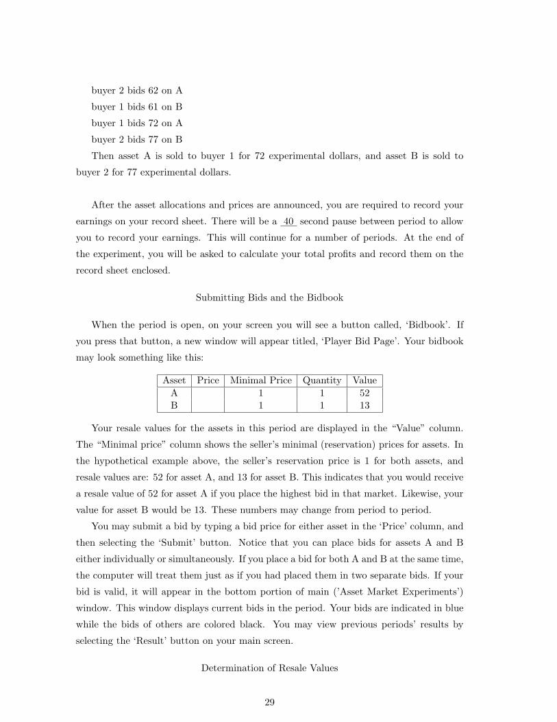
buyer 2 bids 62 on A

buyer 1 bids 61 on B

buyer 1 bids 72 on A

buyer 2 bids 77 on B

Then asset A is sold to buyer 1 for 72 experimental dollars, and asset B is sold to

buyer 2 for 77 experimental dollars.

After the asset allocations and prices are announced, you are required to record your

earnings on your record sheet. There will be a 40 second pause between period to allow

you to record your earnings. This will continue for a number of periods. At the end of

the experiment, you will be asked to calculate your total profits and record them on the

record sheet enclosed.

Submitting Bids and the Bidbook

When the period is open, on your screen you will see a button called, ‘Bidbook’. If

you press that button, a new window will appear titled, ‘Player Bid Page’. Your bidbook

may look something like this:

Asset Price Minimal Price Quantity ValueA 1 1 52B 1 1 13

Your resale values for the assets in this period are displayed in the “Value” column.

The “Minimal price” column shows the seller’s minimal (reservation) prices for assets. In

the hypothetical example above, the seller’s reservation price is 1 for both assets, and

resale values are: 52 for asset A, and 13 for asset B. This indicates that you would receive

a resale value of 52 for asset A if you place the highest bid in that market. Likewise, your

value for asset B would be 13. These numbers may change from period to period.

You may submit a bid by typing a bid price for either asset in the ‘Price’ column, and

then selecting the ‘Submit’ button. Notice that you can place bids for assets A and B

either individually or simultaneously. If you place a bid for both A and B at the same time,

the computer will treat them just as if you had placed them in two separate bids. If your

bid is valid, it will appear in the bottom portion of main (’Asset Market Experiments’)

window. This window displays current bids in the period. Your bids are indicated in blue

while the bids of others are colored black. You may view previous periods’ results by

selecting the ‘Result’ button on your main screen.

Determination of Resale Values

29

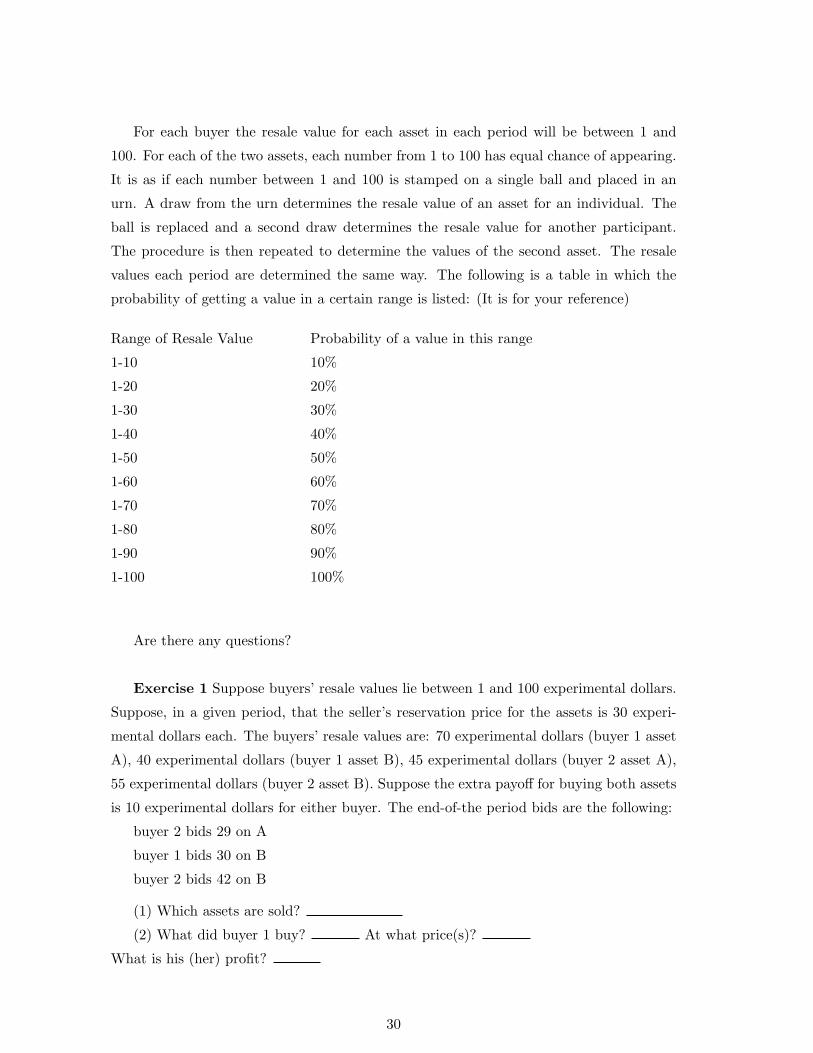
For each buyer the resale value for each asset in each period will be between 1 and

100. For each of the two assets, each number from 1 to 100 has equal chance of appearing.

It is as if each number between 1 and 100 is stamped on a single ball and placed in an

urn. A draw from the urn determines the resale value of an asset for an individual. The

ball is replaced and a second draw determines the resale value for another participant.

The procedure is then repeated to determine the values of the second asset. The resale

values each period are determined the same way. The following is a table in which the

probability of getting a value in a certain range is listed: (It is for your reference)

Range of Resale Value Probability of a value in this range

1-10 10%

1-20 20%

1-30 30%

1-40 40%

1-50 50%

1-60 60%

1-70 70%

1-80 80%

1-90 90%

1-100 100%

Are there any questions?

Exercise 1 Suppose buyers’ resale values lie between 1 and 100 experimental dollars.

Suppose, in a given period, that the seller’s reservation price for the assets is 30 experi-

mental dollars each. The buyers’ resale values are: 70 experimental dollars (buyer 1 asset

A), 40 experimental dollars (buyer 1 asset B), 45 experimental dollars (buyer 2 asset A),

55 experimental dollars (buyer 2 asset B). Suppose the extra payoff for buying both assets

is 10 experimental dollars for either buyer. The end-of-the period bids are the following:

buyer 2 bids 29 on A

buyer 1 bids 30 on B

buyer 2 bids 42 on B

(1) Which assets are sold?

(2) What did buyer 1 buy? At what price(s)?

What is his (her) profit?

30

(3) What did buyer 2 buy? At what price(s)?

What is his (her) profit?

Exercise 2 Suppose buyers’ resale values, the seller’s reservation prices, and the extra

payoff are as given in exercise 1, but the end-of-the period bids are the following:

buyer 2 bids 29 on A

buyer 1 bids 30 on B

buyer 2 bids 42 on B

buyer 2 bids 30 on A

(1) Which assets are sold?

(2) What did buyer 1 buy? At what price(s)?

What is his (her) profit?

(3) What did buyer 2 buy? At what price(s)?

What is his (her) profit?

Period zero will be practice. You will receive no earnings for this period. If you have

a question, please raise your hand and I will come by to answer your question.

Are there any questions?

31

References

[1] Alsemgeest, P., C. Noussair, and M. Olson, 1998. Experimental Comparisons of Auc-

tions Under Single- and Multi-Unit Demand. Economic Inquiry 36, 87-97.

[2] Baldwin, L., R. Marshall and J.-F. Richard, 1997. Bidder collusion at forest service

timber sales. Journal of Political Economy, 105(4), 657-699.

[3] Baldwin, R., and G. Ottaviano, 2001. Multiproduct multinationals and reciprocal

FDI dumping. Journal of International Economics, 54, 429-448.

[4] Brusco, S., and G. Lopomo, 2002. Collusion via signaling in simultaneous ascending

bid auctions with heterogeneous objects, with and without and complementarities.

Review of Economic Studies, 69(2), 407-436.

[5] Bykowsky, M., Cull, R., and J. Ledyard, 2000. Mutually destructive bidding: The

FCC auction design problem. Journal of Regulatory Economics 17(3), 205-228.

[6] Cramton, P. and J.A. Schwartz, 2000. Collusive bidding: lessons from the FCC spec-

trum auctions. Journal of Regulatory Economics, 17(3), 229-252.

[7] Davis, Douglas, and Charles Holt, 1993. Experimental Economics. Princeton Univer-

sity Press.

[8] Dufwenberg, Martin and Uri Gneezy, 2000. Price competition and market concen-

tration: an experimental study. International Journal of Industrial Organization, 18,

7-22.

[9] Federal Communications Commision, 1997. Notice of Apparent Liability for Forfei-

ture. FCC 97-388.

[10] Feinstein, J., M. Block and F. Nold, 1985. Asymmetric information and collusive

behavior in auction markets. American Economic Review, 75(3), 441-460.

[11] Fouraker, L., and S. Sielgel, 1963. Bargaining Behavior. McGraw-Hill, New York.

[12] Graham, D.A. and R.C. Marshall, 1987. Collusive bidder behavior at single-object

second price and English auctions. Journal of Political Economy, 95, 1217-1239.

[13] Grimm, Veronica, and Dirk Engelmann, 2001. Bidding behavior in multi-unit auctions

- an experimental investigation. Mimeo, Humbolt-University of Berlin.

32

[14] Isaac, M.R., Ramey, V. and A.W. Williams, 1984. The effects of market organization

on conspiracies in restraint of trade. Journal of Economic Behavior and Organization,

5, 191-222.

[15] Isaac, M.R. and J. Walker, 1985. Information and conspiracy in sealed bid auctions.

Journal of Economic Behavior and Organization, 6, 139-159.

[16] Jehiel, P., and B. Moldovanu. 2000. License auctions and market structure. University

of Mannheim and University College London discussion paper.

[17] Kagel, John, 1995. Auctions: A Survey of experimental research, in: Kagel, J., and

R. Roth, eds., Handbook of Experimental Economics. Princeton University Press,

501-585.

[18] Kagel, John H. and D. Levin. 2001a. Behavior in Multi-Unit Demand Auctions: Ex-

periments with Uniform price and Dynamic Vickrey Auctions. Econometrica 69(2),

413-454.

[19] Kagel, J. and D. Levin, 2001b. Multi-Unit Demand Auctions with Synergies: Behavior

in Sealed Bid versus Ascending Bid Uniform Price Auctions. Mimeo, Ohio State

University.

[20] Klemperer, Paul. 2000. What really matters in auction design. Mimeo.

[21] Klemperer, Paul. 2002. How (not) to run auctions: The European 3G telecom auc-

tions. European Economic Review 46, 829-845.

[22] Kwasnica, A.M., 2000. The choice of cooperative strategies in sealed bid auctions.

Journal of Economic Behavior and Organization 42(3), 323-346.

[23] Maskin, E., and John Riley, 1996. Uniqueness in Sealed High bid Auctions, unpub-

lished manuscript.

[24] McAfee, R.P. and J. McMillan, 1992. Bidding rings. American Economic Review,

92(3), 579-599.

[25] Meyer, Donald J., Van Huyck, John B., Battalio, Raymond C., and Thomas R.

Saving, 1992. History’s role in coordinating decentralized allocation decisions. Journal

of Political Economy 100(2), 292-316.

[26] Milgrom, P., 1987, Auction theory, In: T. Bewley, (Ed.), Advances of Economic

Theory, Fifth World Congress. Cambridge University Press, pp. 1-32.

33

[27] Milgrom, P., 1998. Game theory and spectrum auctions. European Economic Review,

42, 771-778.

[28] Porter, R.H and J.D. Zona, 1993. Detection of bid rigging in procurement auctions.

Journal of Political Economy, 101(3), 518-538.

[29] Porter, R.H and J.D. Zona, 1999. Ohio school milk markets: an analysis of bidding.

Rand Journal of Economics, 30(2), 263-288.

[30] Selten, R., M. Mitzkewitz, and G. Uhlich, 1997. Duopoly Strategies Programmed by

Experienced Players. Econometrica, 65(3), 517-555.

[31] Sherstyuk, K., 1999. Collusion without conspiracy: an experimental study of one-

sided auctions. Experimental Economics, 2(1), 59-75.

[32] Sherstyuk, K., 2003. On competitive equilibria with common complementarities.

Mathematical Social Sciences, 46(1), 55-62.

[33] Skrzypacz, A., and H. Hopenhayn, 2002. Tacit collusion in repeated auctions. Journal

of Economic Theory, forthcoming.

[34] Tirole, J., 1988. The Theory of Industrial Organization. The MIT Press.

[35] Van Huyck, J., R. Battalio, and R. Beil, 1990. Tacit coordination games, strategic

uncertainty and coordination failure, American Economic Review 80, 234-248.

[36] Van Huyck, J., R. Battalio, and R. Beil, 1991. Strategic uncertainty, equilibrium

selection, and coordination failure in average opinion games, Quarterly Journal of

Economics, 106(3), 885-910.

34

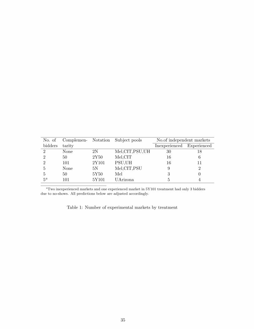
No. of Complemen- Notation Subject pools No.of independent marketsbidders tarity Inexperienced Experienced2 None 2N Mel,CIT,PSU,UH 30 182 50 2Y50 Mel,CIT 16 62 101 2Y101 PSU,UH 16 115 None 5N Mel,CIT,PSU 9 25 50 5Y50 Mel 3 05a 101 5Y101 UArizona 5 4

aTwo inexperienced markets and one experienced market in 5Y101 treatment had only 3 biddersdue to no-shows. All predictions below are adjusted accordingly.

Table 1: Number of experimental markets by treatment

35

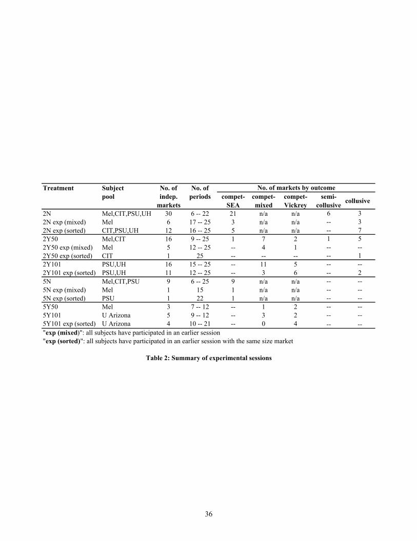
Treatment Subject No. of No. of pool indep.

marketsperiods compet-

SEAcompet-mixed

compet-Vickrey

semi-collusive collusive

2N Mel,CIT,PSU,UH 30 6 -- 22 21 n/a n/a 6 32N exp (mixed) Mel 6 17 -- 25 3 n/a n/a -- 32N exp (sorted) CIT,PSU,UH 12 16 -- 25 5 n/a n/a -- 72Y50 Mel,CIT 16 9 -- 25 1 7 2 1 52Y50 exp (mixed) Mel 5 12 -- 25 -- 4 1 -- --2Y50 exp (sorted) CIT 1 25 -- -- -- -- 12Y101 PSU,UH 16 15 -- 25 -- 11 5 -- --2Y101 exp (sorted) PSU,UH 11 12 -- 25 -- 3 6 -- 25N Mel,CIT,PSU 9 6 -- 25 9 n/a n/a -- --5N exp (mixed) Mel 1 15 1 n/a n/a -- --5N exp (sorted) PSU 1 22 1 n/a n/a -- --5Y50 Mel 3 7 -- 12 -- 1 2 -- --5Y101 U Arizona 5 9 -- 12 -- 3 2 -- --5Y101 exp (sorted) U Arizona 4 10 -- 21 -- 0 4 -- --"exp (mixed)": all subjects have participated in an earlier session"exp (sorted)": all subjects have participated in an earlier session with the same size market

No. of markets by outcome

Table 2: Summary of experimental sessions

36

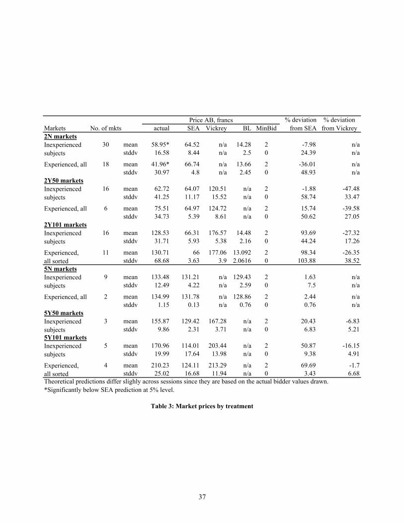
actual SEA Vickrey BL MinBid2N markets

30 mean 58.95* 64.52 n/a 14.28 2 -7.98 n/astddv 16.58 8.44 n/a 2.5 0 24.39 n/a

18 mean 41.96* 66.74 n/a 13.66 2 -36.01 n/astddv 30.97 4.8 n/a 2.45 0 48.93 n/a

2Y50 markets16 mean 62.72 64.07 120.51 n/a 2 -1.88 -47.48

stddv 41.25 11.17 15.52 n/a 0 58.74 33.47

6 mean 75.51 64.97 124.72 n/a 2 15.74 -39.58stddv 34.73 5.39 8.61 n/a 0 50.62 27.05

2Y101 markets16 mean 128.53 66.31 176.57 14.48 2 93.69 -27.32

stddv 31.71 5.93 5.38 2.16 0 44.24 17.26

11 mean 130.71 66 177.06 13.092 2 98.34 -26.35stddv 68.68 3.63 3.9 2.0616 0 103.88 38.52

5N markets9 mean 133.48 131.21 n/a 129.43 2 1.63 n/a

stddv 12.49 4.22 n/a 2.59 0 7.5 n/a

2 mean 134.99 131.78 n/a 128.86 2 2.44 n/astddv 1.15 0.13 n/a 0.76 0 0.76 n/a

5Y50 markets3 mean 155.87 129.42 167.28 n/a 2 20.43 -6.83

stddv 9.86 2.31 3.71 n/a 0 6.83 5.215Y101 markets

5 mean 170.96 114.01 203.44 n/a 2 50.87 -16.15stddv 19.99 17.64 13.98 n/a 0 9.38 4.91

4 mean 210.23 124.11 213.29 n/a 2 69.69 -1.7stddv 25.02 16.68 11.94 n/a 0 3.43 6.68

Experienced, all

Inexperienced subjects

% deviation from VickreyMarkets No. of mkts

Inexperienced subjects

Price AB, francs % deviation from SEA

Table 3: Market prices by treatment

Theoretical predictions differ slighly across sessions since they are based on the actual bidder values drawn. *Significantly below SEA prediction at 5% level.

Experienced, all

Inexperienced subjects

Experienced, all sorted

Experienced, all sorted

Inexperienced subjects

Experienced, all

Inexperienced subjects

Inexperienced subjects

37

Treatment No. mkts Actual Vickrey SEA BL MinBid Rotation Actual Vickrey SEA BL MinBid Rotation2N treatment

30 mean 94.63 n/a 100 92.74 74.18 74.18 47.49 n/a 49.71 80.94 73.71 73.71stddv 4.99 n/a 0 2.04 6.41 6.41 12.29 n/a 5.91 2.72 6.49 6.49

6 mean 97.28 n/a 100 93.08 75.27 75.27 61.39 n/a 48.7 82.3 74.83 74.83stddv 3.14 n/a 0 1.93 6.54 6.54 22.08 n/a 6.23 2.63 6.64 6.64

12 mean 93.74 n/a 100 92.66 75.04 75.04 63.21 n/a 49.34 81.21 74.61 74.61stddv 4.48 n/a 0 2.16 4.07 4.07 22.89 n/a 3.45 2.78 4.15 4.15

2Y50 treatment16 mean 91.17 100 89.26 n/a 54.7 87.21 55.37 25.91 53.05 n/a 54.09 87.05

stddv 4.49 0 1.91 n/a 5.89 4.95 21.63 3.77 5.83 n/a 5.96 5

6 mean 93.31 100 89.14 n/a 54.37 88.53 49.05 25.66 52.4 n/a 53.79 88.4stddv 3.03 0 0.92 n/a 6.02 4.34 20.1 4.63 3.42 n/a 6.1 4.38

2Y101 treatment16 mean 90.35 100 79.61 53.46 43.33 90.58 32.71 19.26 50.83 46.95 42.78 90.5

stddv 6.51 0 1.51 1.86 3.48 3.15 13.63 2.08 3.77 2.28 3.51 3.18

11 mean 94.34 100 80.01 53.9 42.71 91.62 35.68 19.87 51.77 48.05 42.17 91.55stddv 5.34 0 0.92 1.73 2.11 2.32 26.76 2.05 1.52 1.5 2.13 2.35

5N treatment9 mean 98.25 n/a 100 100 59.99 59.99 15.27 n/a 18.84 20.02 59.47 59.47

stddv 1.93 n/a 0 0 0.46 0.46 5.62 n/a 1.11 1.65 0.47 0.47

2 mean 99.64 n/a 100 100 59.72 59.72 16.78 n/a 19.19 21.16 59.21 59.21stddv 0.16 n/a 0 0 0.16 0.16 1.78 n/a 0.85 1.24 0.16 0.16

5Y50 treatment3 mean 96.18 100 85.46 n/a 47.51 73.06 17.9 15.64 20.91 n/a 46.97 72.79

stddv 3.52 0 0.11 n/a 0 0.47 0.65 0.33 0.01 n/a 0.02 0.475Y101 treatment

5 mean 91.35 100 76.39 n/a 37.96 80.85 20.21 14.65 29.58 n/a 37.67 80.93stddv 5.5 0 6.63 n/a 0.83 2.41 5.85 2.88 11.44 n/a 1.07 2.75

4 mean 97.16 100 73 n/a 38.94 79.74 13.33 14.71 24.08 n/a 38.59 79.72stddv 2.11 0 2.24 n/a 1.61 2.74 8.39 2.35 7.38 n/a 1.87 3.03

* Theoretical predictions differ slighly across sessions since they are based on the actual bidder values drawn

Experienced, all sorted

Experienced, all sorted

Inexperienced subjects

Experienced, all

Inexperienced subjects

Table 4: Efficiency and bidder gains by treatment

Efficiency, percent Relative gains, percent

Inexperienced subjects

Experienced, mixed

Experienced, sorted

Inexperienced subjects

Experienced, all

Inexperienced subjects

Inexperienced subjects

38

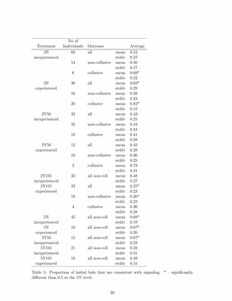
No ofTreatment Individuals Outcome Average

2N 60 all mean 0.52inexperienced stddv 0.27

54 non-collusive mean 0.50stddv 0.27

6 collusive mean 0.69*stddv 0.22

2N 36 all mean 0.63*experienced stddv 0.29

16 non-collusive mean 0.38stddv 0.22

20 collusive mean 0.82*stddv 0.15

2Y50 32 all mean 0.43inexperienced stddv 0.25

22 non-collusive mean 0.43stddv 0.24

10 collusive mean 0.41stddv 0.28

2Y50 12 all mean 0.42experienced stddv 0.28

10 non-collusive mean 0.36stddv 0.25

2 collusive mean 0.73stddv 0.21

2Y101 32 all non-coll mean 0.48inexperienced stddv 0.27

2Y101 22 all mean 0.27*experienced stddv 0.23

18 non-collusive mean 0.26*stddv 0.22

4 collusive mean 0.30stddv 0.28

5N 45 all non-coll mean 0.68*inexperienced stddv 0.19

5N 10 all non-coll mean 0.67*experienced stddv 0.20

5Y50 15 all non-coll mean 0.67*inexperienced stddv 0.22

5Y101 21 all non-coll mean 0.59inexperienced stddv 0.21

5Y101 18 all non-coll mean 0.49experienced stddv 0.31

Table 5: Proportion of initial bids that are consistent with signaling. * – significantlydifferent than 0.5 at the 5% level.

39

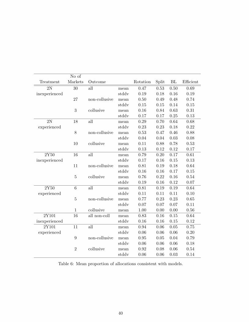
No ofTreatment Markets Outcome Rotation Split BL Efficient

2N 30 all mean 0.47 0.53 0.50 0.69inexperienced stddv 0.19 0.18 0.16 0.19

27 non-collusive mean 0.50 0.49 0.48 0.74stddv 0.15 0.15 0.14 0.15

3 collusive mean 0.16 0.84 0.63 0.31stddv 0.17 0.17 0.25 0.13

2N 18 all mean 0.29 0.70 0.64 0.68experienced stddv 0.23 0.23 0.18 0.22

8 non-collusive mean 0.53 0.47 0.46 0.88stddv 0.04 0.04 0.03 0.08

10 collusive mean 0.11 0.88 0.78 0.53stddv 0.13 0.12 0.12 0.17

2Y50 16 all mean 0.79 0.20 0.17 0.61inexperienced stddv 0.17 0.16 0.15 0.13

11 non-collusive mean 0.81 0.19 0.18 0.64stddv 0.16 0.16 0.17 0.15

5 collusive mean 0.76 0.22 0.16 0.54stddv 0.19 0.16 0.12 0.07

2Y50 6 all mean 0.81 0.19 0.19 0.64experienced stddv 0.11 0.11 0.11 0.10

5 non-collusive mean 0.77 0.23 0.23 0.65stddv 0.07 0.07 0.07 0.11

1 collusive mean 1.00 0.00 0.00 0.562Y101 16 all non-coll mean 0.83 0.16 0.15 0.64

inexperienced stddv 0.16 0.16 0.15 0.122Y101 11 all mean 0.94 0.06 0.05 0.75

experienced stddv 0.06 0.06 0.06 0.209 non-collusive mean 0.95 0.05 0.04 0.79

stddv 0.06 0.06 0.06 0.182 collusive mean 0.92 0.08 0.06 0.54

stddv 0.06 0.06 0.03 0.14

Table 6: Mean proportion of allocations consistent with models.

40

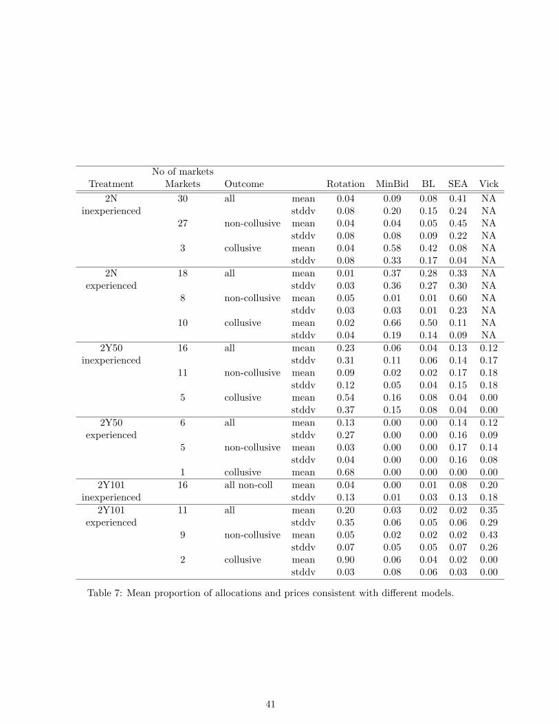
No of marketsTreatment Markets Outcome Rotation MinBid BL SEA Vick

2N 30 all mean 0.04 0.09 0.08 0.41 NAinexperienced stddv 0.08 0.20 0.15 0.24 NA

27 non-collusive mean 0.04 0.04 0.05 0.45 NAstddv 0.08 0.08 0.09 0.22 NA

3 collusive mean 0.04 0.58 0.42 0.08 NAstddv 0.08 0.33 0.17 0.04 NA

2N 18 all mean 0.01 0.37 0.28 0.33 NAexperienced stddv 0.03 0.36 0.27 0.30 NA

8 non-collusive mean 0.05 0.01 0.01 0.60 NAstddv 0.03 0.03 0.01 0.23 NA

10 collusive mean 0.02 0.66 0.50 0.11 NAstddv 0.04 0.19 0.14 0.09 NA

2Y50 16 all mean 0.23 0.06 0.04 0.13 0.12inexperienced stddv 0.31 0.11 0.06 0.14 0.17

11 non-collusive mean 0.09 0.02 0.02 0.17 0.18stddv 0.12 0.05 0.04 0.15 0.18

5 collusive mean 0.54 0.16 0.08 0.04 0.00stddv 0.37 0.15 0.08 0.04 0.00

2Y50 6 all mean 0.13 0.00 0.00 0.14 0.12experienced stddv 0.27 0.00 0.00 0.16 0.09

5 non-collusive mean 0.03 0.00 0.00 0.17 0.14stddv 0.04 0.00 0.00 0.16 0.08

1 collusive mean 0.68 0.00 0.00 0.00 0.002Y101 16 all non-coll mean 0.04 0.00 0.01 0.08 0.20

inexperienced stddv 0.13 0.01 0.03 0.13 0.182Y101 11 all mean 0.20 0.03 0.02 0.02 0.35

experienced stddv 0.35 0.06 0.05 0.06 0.299 non-collusive mean 0.05 0.02 0.02 0.02 0.43

stddv 0.07 0.05 0.05 0.07 0.262 collusive mean 0.90 0.06 0.04 0.02 0.00

stddv 0.03 0.08 0.06 0.03 0.00

Table 7: Mean proportion of allocations and prices consistent with different models.

41

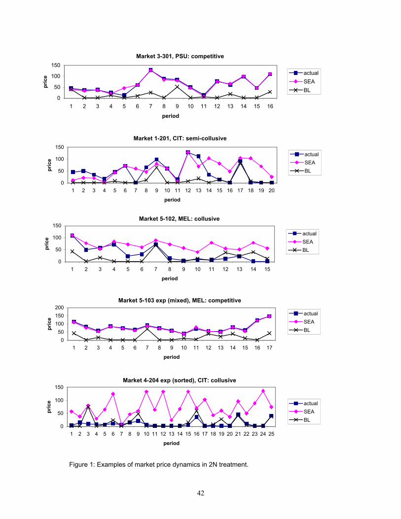
Figure 1: Examples of market price dynamics in 2N treatment.

Market 3-301, PSU: competitive

0

50

100

150

1 2 3 4 5 6 7 8 9 10 11 12 13 14 15 16

period

pric

e actualSEABL

Market 1-201, CIT: semi-collusive

0

50

100

150

1 2 3 4 5 6 7 8 9 10 11 12 13 14 15 16 17 18 19 20

period

pric

e

actualSEABL

Market 5-102, MEL: collusive

0

50

100

150

1 2 3 4 5 6 7 8 9 10 11 12 13 14 15

period

pric

e

actualSEABL

Market 4-204 exp (sorted), CIT: collusive

0

50

100

150

1 2 3 4 5 6 7 8 9 10 11 12 13 14 15 16 17 18 19 20 21 22 23 24 25

period

pric

e actualSEABL

Market 5-103 exp (mixed), MEL: competitive

050

100150200

1 2 3 4 5 6 7 8 9 10 11 12 13 14 15 16 17

period

pric

e

actualSEABL

42

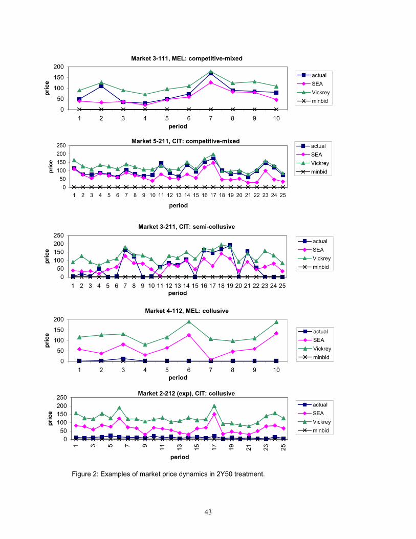
Figure 2: Examples of market price dynamics in 2Y50 treatment.

Market 3-111, MEL: competitive-mixed

0

50

100

150

200

1 2 3 4 5 6 7 8 9 10period

pric

e

actualSEAVickreyminbid

Market 5-211, CIT: competitive-mixed

050

100150200250

1 2 3 4 5 6 7 8 9 10 11 12 13 14 15 16 17 18 19 20 21 22 23 24 25

period

pric

e

actualSEAVickreyminbid

Market 3-211, CIT: semi-collusive

050

100150200250

1 2 3 4 5 6 7 8 9 10 11 12 13 14 15 16 17 18 19 20 21 22 23 24 25period

pric

e

actualSEAVickreyminbid

Market 4-112, MEL: collusive

0

50100

150

200

1 2 3 4 5 6 7 8 9 10period

pric

e actualSEAVickreyminbid

Market 2-212 (exp), CIT: collusive

050

100150200250

1 3 5 7 9 11 13 15 17 19 21 23 25

period

pric

e

actualSEAVickreyminbid

43

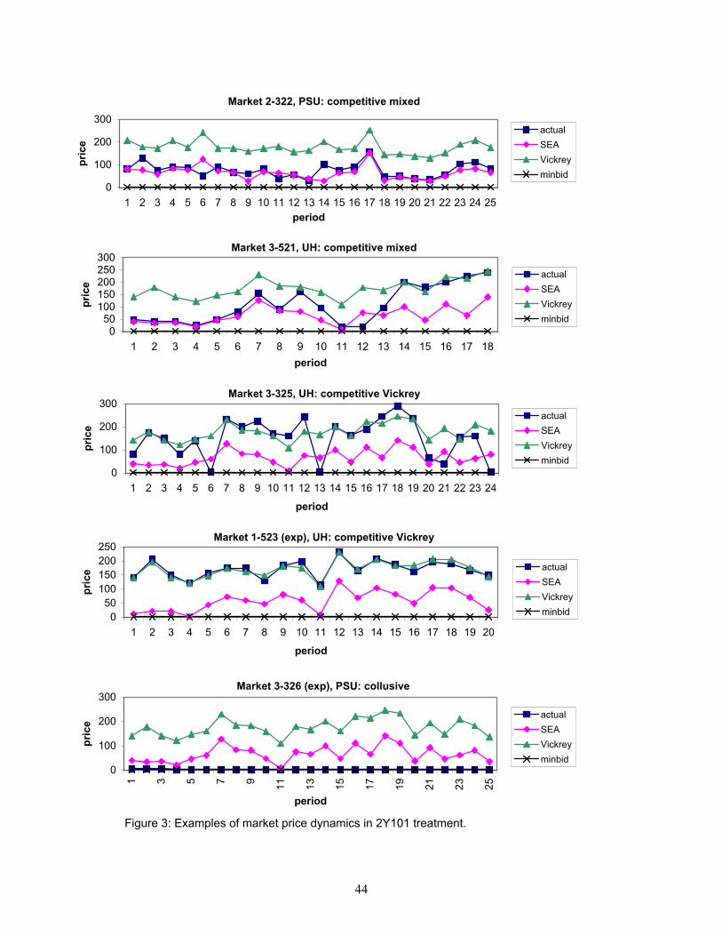
Figure 3: Examples of market price dynamics in 2Y101 treatment.

Market 2-322, PSU: competitive mixed

0

100

200

300

1 2 3 4 5 6 7 8 9 10 11 12 13 14 15 16 17 18 19 20 21 22 23 24 25period

pric

e

actualSEAVickreyminbid

Market 3-521, UH: competitive mixed

050

100150200250300

1 2 3 4 5 6 7 8 9 10 11 12 13 14 15 16 17 18period

pric

e

actualSEAVickreyminbid

Market 3-325, UH: competitive Vickrey

0

100

200

300

1 2 3 4 5 6 7 8 9 10 11 12 13 14 15 16 17 18 19 20 21 22 23 24

period

pric

e

actualSEAVickreyminbid

Market 1-523 (exp), UH: competitive Vickrey

050

100150200250

1 2 3 4 5 6 7 8 9 10 11 12 13 14 15 16 17 18 19 20

period

pric

e actualSEAVickreyminbid

Market 3-326 (exp), PSU: collusive

0

100

200

300

1 3 5 7 9 11 13 15 17 19 21 23 25

period

pric

e

actualSEAVickreyminbid

44

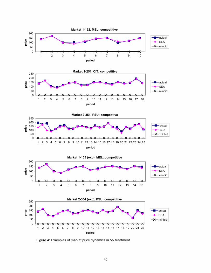
Figure 4: Examples of market price dynamics in 5N treatment.

Market 1-152, MEL: competitive

050

100150200

1 2 3 4 5 6 7 8 9 10

period

pric

e

actualSEAminbid

Market 1-251, CIT: competitive

050

100150200250

1 2 3 4 5 6 7 8 9 10 11 12 13 14 15 16 17 18

period

pric

e actualSEAminbid

Market 2-351, PSU: competitive

050

100150200250

1 2 3 4 5 6 7 8 9 10 11 12 13 14 15 16 17 18 19 20 21 22 23 24 25

period

pric

e actualSEAminbid

Market 1-153 (exp), MEL: competitive

0

50

100

150

200

1 2 3 4 5 6 7 8 9 10 11 12 13 14 15

period

pric

e

actualSEAminbid

Market 2-354 (exp), PSU: competitive

050

100150200250

1 2 3 4 5 6 7 8 9 10 11 12 13 14 15 16 17 18 19 20 21 22

period

pric

e actualSEAminbid

45

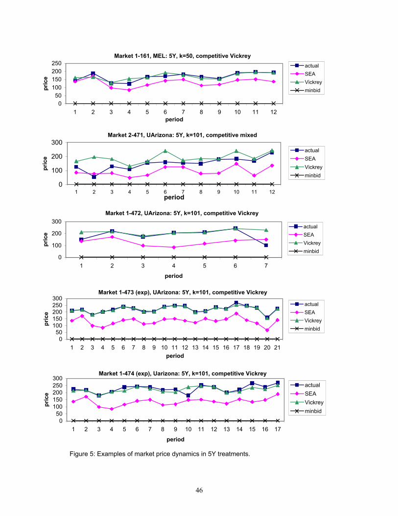
Figure 5: Examples of market price dynamics in 5Y treatments.

Market 1-161, MEL: 5Y, k=50, competitive Vickrey

050

100150200250

1 2 3 4 5 6 7 8 9 10 11 12period

pric

e

actualSEAVickreyminbid

Market 1-472, UArizona: 5Y, k=101, competitive Vickrey

0

100

200

300

1 2 3 4 5 6 7

period

pric

e

actualSEAVickreyminbid

Market 1-473 (exp), UArizona: 5Y, k=101, competitive Vickrey

050

100150200250300

1 2 3 4 5 6 7 8 9 10 11 12 13 14 15 16 17 18 19 20 21period

pric

e

actualSEAVickreyminbid

Market 2-471, UArizona: 5Y, k=101, competitive mixed

0

100

200

300

1 2 3 4 5 6 7 8 9 10 11 12period

pric

e

actualSEAVickreyminbid

Market 1-474 (exp), Uarizona: 5Y, k=101, competitive Vickrey

050

100150200250300

1 2 3 4 5 6 7 8 9 10 11 12 13 14 15 16 17

period

pric

e

actualSEAVickreyminbid

46