Embed Size (px)
Citation preview

Introduction Colorful Functions Series Conclusions
Colorful visualization of complex functions
Levente Lócsi
Department of Numerical Analysis, Faculty of Informatics,Eötvös Loránd University, Budapest, Hungary
NuHAG SeminarVienna, April 6, 2011

Introduction Colorful Functions Series Conclusions
Motivation – What are these?

Introduction Colorful Functions Series Conclusions
Motivation – History & Possible future work

Introduction Colorful Functions Series Conclusions
Table of Contents
Introduction
’Colorful’ plots
Discussion of some functions
Function series
Conclusions

Introduction Colorful Functions Series Conclusions
Table of Contents
Introduction
’Colorful’ plots
Discussion of some functions
Function series
Conclusions

Introduction Colorful Functions Series Conclusions
Plotting R → R functions

Introduction Colorful Functions Series Conclusions
Complex numbers & arithmetic
Re
Im
ϕ
yz = x + iy
x
r
Re
Im
z1
z2
z1 + z2
Re
Im
ϕ1
z1ϕ2z2
ϕ1 + ϕ2
z1 · z2
Re
Im
z
z

Introduction Colorful Functions Series Conclusions
Complex plots – Two planes
f (z) = z2

Introduction Colorful Functions Series Conclusions
Complex plots – Two planes
f (z) = exp z = ez = ex+iy = ex · eiy = ex (cos y + i sin y)

Introduction Colorful Functions Series Conclusions
Complex plots – Vectorfields
f (z) = z2 − 1

Introduction Colorful Functions Series Conclusions
Complex plots – Vectorfields
f (z) = exp z

Introduction Colorful Functions Series Conclusions
Complex plots – 3D (2 × R2 → R)
f1(x , y) = x2 − y2 f2(x , y) = 2xy
f (z) = z2

Introduction Colorful Functions Series Conclusions
Complex plots – 3D (2 × R2 → R)
f1(x , y) = ex cos y f2(x , y) = ex sin yf (z) = exp z

Introduction Colorful Functions Series Conclusions
Complex plots – One image (complexplot)
f (z) = z2

Introduction Colorful Functions Series Conclusions
Complex plots – One image (complexplot)
f (z) = exp z

Introduction Colorful Functions Series Conclusions
Complex plots – One image (complexplot)
f (z) = sin z

Introduction Colorful Functions Series Conclusions
Complex plots – Fractal coloring
The Mandelbrot set

Introduction Colorful Functions Series Conclusions
Table of Contents
Introduction
’Colorful’ plots
Discussion of some functions
Function series
Conclusions

Introduction Colorful Functions Series Conclusions
The idea of ’colorful’ plotting
• Assign unique colors to complex numbers
• C → B3, with B = [0..255], RGB
• Plot f : C → C by painting the pixels on a plane (on a square/ interval) the color assigned to the value f(z)
• Different colorings. . .

Introduction Colorful Functions Series Conclusions
The idea of ’colorful’ plotting
• Assign unique colors to complex numbers
• C → B3, with B = [0..255], RGB
• Plot f : C → C by painting the pixels on a plane (on a square/ interval) the color assigned to the value f(z)
• Different colorings. . .

Introduction Colorful Functions Series Conclusions
The idea of ’colorful’ plotting
• Assign unique colors to complex numbers
• C → B3, with B = [0..255], RGB
• Plot f : C → C by painting the pixels on a plane (on a square/ interval) the color assigned to the value f(z)
• Different colorings. . .

Introduction Colorful Functions Series Conclusions
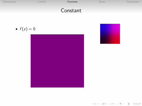
Example coloring: ImRe
• Treat the real and imaginary part separately
• R → B (e.g. red and blue)
• In other words:
• Note: we already have the plot of f (z) = z

Introduction Colorful Functions Series Conclusions
Colorings
• </=, magnitude / argument

Introduction Colorful Functions Series Conclusions
Advantages & disadvantages
• Concise, perspicuous (’übersichtlich’)
• Beautyful
• ’Waste of paint’

Introduction Colorful Functions Series Conclusions
Table of Contents
Introduction
’Colorful’ plots
Discussion of some functions
Function series
Conclusions
Introduction Colorful Functions Series Conclusions
Functions
• f (z)
Introduction Colorful Functions Series Conclusions
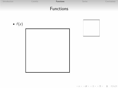
Constant
• f (z) = 0
Introduction Colorful Functions Series Conclusions
Identity
• f (z) = z

Introduction Colorful Functions Series Conclusions
Conjugate – 1
• f (z) = z

Introduction Colorful Functions Series Conclusions
Conjugate – 2
• f (z) = z

Introduction Colorful Functions Series Conclusions
Linear
• f (z) = (2 + i)z + 2

Introduction Colorful Functions Series Conclusions
Square – 1
• f (z) = z2

Introduction Colorful Functions Series Conclusions
Square – 2
• f (z) = z2

Introduction Colorful Functions Series Conclusions
Square – 3
• f (z) = z2

Introduction Colorful Functions Series Conclusions
A polynomial of degree two
• f (z) = z2 − 1

Introduction Colorful Functions Series Conclusions
Polynomials of degree two – animation
• Let f (z) = (z − t0)(z + t0), where
• t0 = eiϕ, ϕ ∈ [0..π].
Re
Im
t0
−t0

Introduction Colorful Functions Series Conclusions
Polynomials of degree two – animation
Please download video by clicking here.
Or use this url:http://locsi.web.elte.hu/complex/doc/k_video1_negyzetes.avi

Introduction Colorful Functions Series Conclusions
A polynomial of degree three – 1
• f (z) = (z − 2)(z + i)(z + 2 − i)
Introduction Colorful Functions Series Conclusions
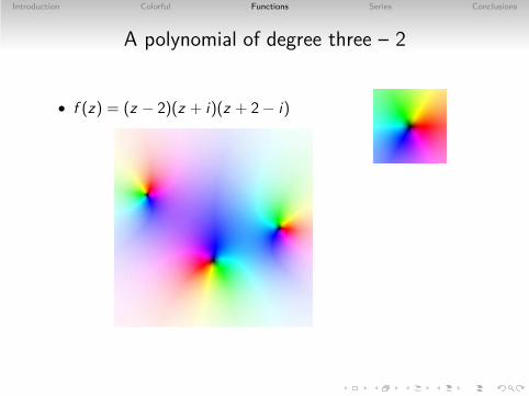
A polynomial of degree three – 2
• f (z) = (z − 2)(z + i)(z + 2 − i)

Introduction Colorful Functions Series Conclusions
And yet another one
• f (z) = (z − 2)(z + 1)2

Introduction Colorful Functions Series Conclusions
Exponential – 1
• f (z) = exp z

Introduction Colorful Functions Series Conclusions
Exponential – 2
• f (z) = exp z

Introduction Colorful Functions Series Conclusions
Sine
• f (z) = sin z

Introduction Colorful Functions Series Conclusions
Square root – 1
• f (z) =√
z (principal branch)

Introduction Colorful Functions Series Conclusions
Square root – 2
• f (z) =√
z (principal branch)

Introduction Colorful Functions Series Conclusions
Square root branches – animation
• Invert the square function restricted to different domains
• Where is the (branch) cut / the jump?
Re
Im
Re
Im

Introduction Colorful Functions Series Conclusions
Square root branches – animation
Please download video by clicking here.
Or use this url:http://locsi.web.elte.hu/complex/doc/k_video2_gyokagak.avi

Introduction Colorful Functions Series Conclusions
Logarithm
• f (z) = log z (principal branch)

Introduction Colorful Functions Series Conclusions
Logarithm branches – animation
• Invert the exponential function restricted to different domains
• Where is the cut / jump?
Re
Im
Re
Im

Introduction Colorful Functions Series Conclusions
Logarithm branches – animation
Please download video by clicking here.
Or use this url:http://locsi.web.elte.hu/complex/doc/k_video3_logagak.avi

Introduction Colorful Functions Series Conclusions
Inversion – 1
• f (z) = 1/z

Introduction Colorful Functions Series Conclusions
Inversion – 2
• f (z) = 1/z

Introduction Colorful Functions Series Conclusions
Reciprocal
• f (z) = 1/z = (1/z)

Introduction Colorful Functions Series Conclusions
A pole of order two – 1
• f (z) = 1/z2

Introduction Colorful Functions Series Conclusions
A pole of order two – 2
• f (z) = 1/z2

Introduction Colorful Functions Series Conclusions
Of singularities
Laurent series
+∞∑
k=−∞
ck(z − a)k
Order of the pole ∼ smallest (negative) index of terms withnon-zero coefficient (if there are finitely many of such)Essential singularity ∼ infinite number of such terms exist
Picard’s theorem
May f : C → C have an essential singularity at a ∈ C. Then:∃w0 ∈ C : ∀ε > 0 : ∀w ∈ C \ {w0} : ∃z ∈ kε(a) : f (z) = w .
Introduction Colorful Functions Series Conclusions
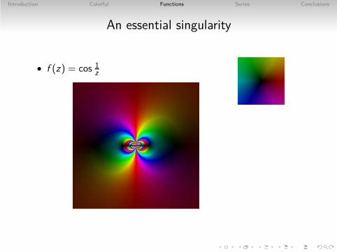
An essential singularity
• f (z) = cos 1z

Introduction Colorful Functions Series Conclusions
A linear fraction
• f (z) = (z − 2)/(z + 2) (Zhukovsky)

Introduction Colorful Functions Series Conclusions
Table of Contents
Introduction
’Colorful’ plots
Discussion of some functions
Function series
Conclusions

Introduction Colorful Functions Series Conclusions
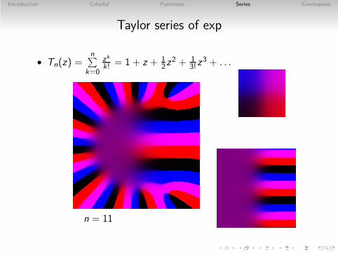
Taylor series of exp
• Tn(z) =n∑
k=0
zk
k! = 1 + z + 12z2 + 1
3!z3 + . . .
n =

Introduction Colorful Functions Series Conclusions
Taylor series of exp
• Tn(z) =n∑
k=0
zk
k! = 1 + z + 12z2 + 1
3!z3 + . . .
n = 0

Introduction Colorful Functions Series Conclusions
Taylor series of exp
• Tn(z) =n∑
k=0
zk
k! = 1 + z + 12z2 + 1
3!z3 + . . .
n = 1

Introduction Colorful Functions Series Conclusions
Taylor series of exp
• Tn(z) =n∑
k=0
zk
k! = 1 + z + 12z2 + 1
3!z3 + . . .
n = 2

Introduction Colorful Functions Series Conclusions
Taylor series of exp
• Tn(z) =n∑
k=0
zk
k! = 1 + z + 12z2 + 1
3!z3 + . . .
n = 3

Introduction Colorful Functions Series Conclusions
Taylor series of exp
• Tn(z) =n∑
k=0
zk
k! = 1 + z + 12z2 + 1
3!z3 + . . .
n = 4

Introduction Colorful Functions Series Conclusions
Taylor series of exp
• Tn(z) =n∑
k=0
zk
k! = 1 + z + 12z2 + 1
3!z3 + . . .
n = 5

Introduction Colorful Functions Series Conclusions
Taylor series of exp
• Tn(z) =n∑
k=0
zk
k! = 1 + z + 12z2 + 1
3!z3 + . . .
n = 6

Introduction Colorful Functions Series Conclusions
Taylor series of exp
• Tn(z) =n∑
k=0
zk
k! = 1 + z + 12z2 + 1
3!z3 + . . .
n = 7

Introduction Colorful Functions Series Conclusions
Taylor series of exp
• Tn(z) =n∑
k=0
zk
k! = 1 + z + 12z2 + 1
3!z3 + . . .
n = 8

Introduction Colorful Functions Series Conclusions
Taylor series of exp
• Tn(z) =n∑
k=0
zk
k! = 1 + z + 12z2 + 1
3!z3 + . . .
n = 9

Introduction Colorful Functions Series Conclusions
Taylor series of exp
• Tn(z) =n∑
k=0
zk
k! = 1 + z + 12z2 + 1
3!z3 + . . .
n = 10
Introduction Colorful Functions Series Conclusions
Taylor series of exp
• Tn(z) =n∑
k=0
zk
k! = 1 + z + 12z2 + 1
3!z3 + . . .
n = 11

Introduction Colorful Functions Series Conclusions
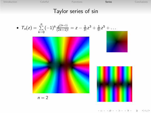
Taylor series of sin
• Tn(z) =n∑
k=0(−1)k z (2k+1)
(2k+1)! = z − 13!z
3 + 15!z
5 + . . .
n =

Introduction Colorful Functions Series Conclusions
Taylor series of sin
• Tn(z) =n∑
k=0(−1)k z (2k+1)
(2k+1)! = z − 13!z
3 + 15!z
5 + . . .
n = 0

Introduction Colorful Functions Series Conclusions
Taylor series of sin
• Tn(z) =n∑
k=0(−1)k z (2k+1)
(2k+1)! = z − 13!z
3 + 15!z
5 + . . .
n = 1
Introduction Colorful Functions Series Conclusions
Taylor series of sin
• Tn(z) =n∑
k=0(−1)k z (2k+1)
(2k+1)! = z − 13!z
3 + 15!z
5 + . . .
n = 2

Introduction Colorful Functions Series Conclusions
Taylor series of sin
• Tn(z) =n∑
k=0(−1)k z (2k+1)
(2k+1)! = z − 13!z
3 + 15!z
5 + . . .
n = 3

Introduction Colorful Functions Series Conclusions
Taylor series of sin
• Tn(z) =n∑
k=0(−1)k z (2k+1)
(2k+1)! = z − 13!z
3 + 15!z
5 + . . .
n = 4

Introduction Colorful Functions Series Conclusions
Taylor series of sin
• Tn(z) =n∑
k=0(−1)k z (2k+1)
(2k+1)! = z − 13!z
3 + 15!z
5 + . . .
n = 5

Introduction Colorful Functions Series Conclusions
Taylor series of sin
• Tn(z) =n∑
k=0(−1)k z (2k+1)
(2k+1)! = z − 13!z
3 + 15!z
5 + . . .
n = 6

Introduction Colorful Functions Series Conclusions
Taylor series of sin
• Tn(z) =n∑
k=0(−1)k z (2k+1)
(2k+1)! = z − 13!z
3 + 15!z
5 + . . .
n = 7

Introduction Colorful Functions Series Conclusions
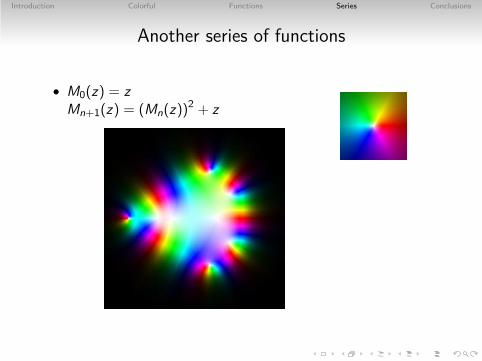
Another series of functions
• M0(z) = zMn+1(z) = (Mn(z))
2 + z

Introduction Colorful Functions Series Conclusions
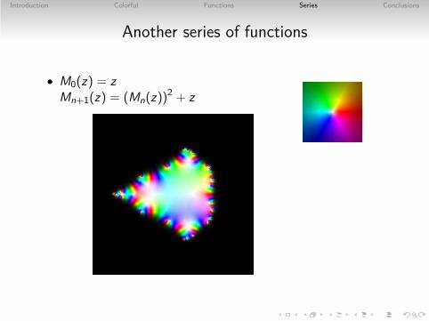
Another series of functions
• M0(z) = zMn+1(z) = (Mn(z))
2 + z

Introduction Colorful Functions Series Conclusions
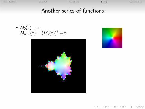
Another series of functions
• M0(z) = zMn+1(z) = (Mn(z))
2 + z

Introduction Colorful Functions Series Conclusions
Another series of functions
• M0(z) = zMn+1(z) = (Mn(z))
2 + z
Introduction Colorful Functions Series Conclusions
Another series of functions
• M0(z) = zMn+1(z) = (Mn(z))
2 + z

Introduction Colorful Functions Series Conclusions
Another series of functions
• M0(z) = zMn+1(z) = (Mn(z))
2 + z
Introduction Colorful Functions Series Conclusions
Another series of functions
• M0(z) = zMn+1(z) = (Mn(z))
2 + z

Introduction Colorful Functions Series Conclusions
Another series of functions
• M0(z) = zMn+1(z) = (Mn(z))
2 + z

Introduction Colorful Functions Series Conclusions
Another series of functions
• M0(z) = zMn+1(z) = (Mn(z))
2 + z

Introduction Colorful Functions Series Conclusions
Another series of functions
• M0(z) = zMn+1(z) = (Mn(z))
2 + z
Introduction Colorful Functions Series Conclusions
Another series of functions
• M0(z) = zMn+1(z) = (Mn(z))
2 + z

Introduction Colorful Functions Series Conclusions
Table of Contents
Introduction
’Colorful’ plots
Discussion of some functions
Function series
Conclusions

Introduction Colorful Functions Series Conclusions
Conclusions
• A small (non-complete) discussion of complex functions
• Idea and validity of ’colorful’ visualization
• No implementation known with different colorings availableand easy to use
• Matlab implementation, Gabor transforms
• Exam ,

Introduction Colorful Functions Series Conclusions
Conclusions
• A small (non-complete) discussion of complex functions
• Idea and validity of ’colorful’ visualization
• No implementation known with different colorings availableand easy to use
• Matlab implementation, Gabor transforms
• Exam ,

Introduction Colorful Functions Series Conclusions
Conclusions
• A small (non-complete) discussion of complex functions
• Idea and validity of ’colorful’ visualization
• No implementation known with different colorings availableand easy to use
• Matlab implementation, Gabor transforms
• Exam ,

Introduction Colorful Functions Series Conclusions
Exam – Question 1
Introduction Colorful Functions Series Conclusions
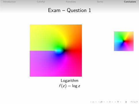
Exam – Question 1
Logarithmf (z) = log z

Introduction Colorful Functions Series Conclusions
Exam – Question 2

Introduction Colorful Functions Series Conclusions
Exam – Question 2
A polinomial of degree five with one root of multiplicity two andthree roots of multiplicity one
f (z) = i(z − i)2(z + i)(z − 1 − 310 i)(z + 1 − 3
10 i)

Introduction Colorful Functions Series Conclusions
Exam – Question 3

Introduction Colorful Functions Series Conclusions
Exam – Question 3
Tangentf (z) = sin z/ cos z

Introduction Colorful Functions Series Conclusions
Exam – Question 4
Introduction Colorful Functions Series Conclusions
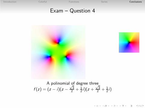
Exam – Question 4
A polinomial of degree three
f (z) = (z − i)(z −√
32 + 1
2 i)(z +√
32 + 1
2 i)

Introduction Colorful Functions Series Conclusions
Exam – Question 5

Introduction Colorful Functions Series Conclusions
Exam – Question 5
A function with a zero of multiplicity one and a pole of order twof (z) = 1/z2 − iz

Introduction Colorful Functions Series Conclusions
Exam – Question 6

Introduction Colorful Functions Series Conclusions
Exam – Question 6
f (z) = exp cos z

Introduction Colorful Functions Series Conclusions
Exam – Question 6
f (z) = exp cos z

Introduction Colorful Functions Series Conclusions
What are these?

Introduction Colorful Functions Series Conclusions
References
• See WWW
• References on my homepage(as soon as it’s translated and broken links are fixed)

Introduction Colorful Functions Series Conclusions
Colorful visualization of complex functions
Author: Levente Lócsi
Occasion: NuHAG SeminarVienna, April 8, 2011
Web: http://locsi.web.elte.hu/complex/E-mail: [email protected]


![Functions of a Complex Variable[1]](https://img.pdfslide.net/doc/110x75/577d23ac1a28ab4e1e9a756a/functions-of-a-complex-variable1.jpg)