Embed Size (px)
Citation preview
HAL Id: tel-00995041https://tel.archives-ouvertes.fr/tel-00995041
Submitted on 22 May 2014
HAL is a multi-disciplinary open accessarchive for the deposit and dissemination of sci-entific research documents, whether they are pub-lished or not. The documents may come fromteaching and research institutions in France orabroad, or from public or private research centers.
L’archive ouverte pluridisciplinaire HAL, estdestinée au dépôt et à la diffusion de documentsscientifiques de niveau recherche, publiés ou non,émanant des établissements d’enseignement et derecherche français ou étrangers, des laboratoirespublics ou privés.
Coloring, packing and embedding of graphsMohammed Amin Tahraoui
To cite this version:Mohammed Amin Tahraoui. Coloring, packing and embedding of graphs. Other [cs.OH]. UniversitéClaude Bernard - Lyon I, 2012. English. �NNT : 2012LYO10278�. �tel-00995041�
Numéro d’ordre: ***** Année 2012
Université Claude Bernard Lyon 1
Laboratoire d’InfoRmatique en Image et Systèmesd’information
École Doctorale Informatique et Mathématiques de Lyon
Thèse de l’Université de Lyon
Présentée en vue d’obtenir le grade de Docteur,
spécialité Informatique
par
Mohammed Amin TAHRAOUI
Coloring, Packing and Embedding of
graphs
Thèse soutenue le 04/12/2012 devant le jury composé de:
Rapporteurs: Daniela Grigori – Professeur à l’Université de Paris Dauphine
Eric Sopena – Professeur à l’Université de Bordeaux 1
Examinateurs: Sylvain Gravier – DR CNRS à l’Université de Grenoble 1
Directeur: Hamamache Kheddouci – Professeur à l’Université de Lyon 1
Co-directeur: Eric Duchêne – Maitre de Conférences à l’Université de Lyon 1
ii
Acknowledgments
First of all I indebted to my supervisor Hamamache Kheddouci for his helpful guid-
ance and advice for the entirety of my graduate studies. I would also like to thank
him for introducing me to the topic of graph theory and for many useful discussions
(mathematical and otherwise).
I also would like to express my deepest acknowledgement to the other supervisor
Prof. Eric Duchêne for his inspiring guidance, helpful suggestions, and persistent
encouragement as well as close and constant supervision throughout the period of
my PhD.
Many thanks go to Prof. Daniela Grigori and Prof. Eric Sopena for being the
reviewers of my thesis and for their valuable comments and constructive suggestions
on the thesis.
I am grateful to the members of defense committee: Prof. Daniela Grigori, Prof.
Eric Sopena, Prof. Sylvain Gravier, Prof. Hamamache Kheddouci and Prof. Eric
Duchêne for their friendship and wisdom.
I especially thank all my lab friends, whose wonderful presence made it a con-
vivial place to work.
I warmly thank all my friends who were always supporting and encouraging me
with their best wishes.
Finally, I express my love and gratitude to my parents and my sisters. This
thesis would not have been possible without their inseparable support, love and
persistent confidence in me.
Contents
1 Introduction 1
2 Preliminaries 5
2.1 Basic notations . . . . . . . . . . . . . . . . . . . . . . . . . . . . . . 5
2.2 Some graph operations . . . . . . . . . . . . . . . . . . . . . . . . . . 6
2.3 Some families of graphs . . . . . . . . . . . . . . . . . . . . . . . . . 7
I Graph Coloring Problem 11
3 Vertex-Distinguishing Edge Coloring of Graphs 13
3.1 Introduction to graph coloring . . . . . . . . . . . . . . . . . . . . . . 13
3.1.1 Vertex coloring problem . . . . . . . . . . . . . . . . . . . . . 14
3.1.2 Edge coloring problem . . . . . . . . . . . . . . . . . . . . . . 15
3.1.3 Total coloring problem . . . . . . . . . . . . . . . . . . . . . . 16
3.2 Vertex-distinguishing edge coloring . . . . . . . . . . . . . . . . . . . 16
3.2.1 Variations of the problem . . . . . . . . . . . . . . . . . . . . 17
3.2.2 Strong edge coloring . . . . . . . . . . . . . . . . . . . . . . . 17
3.2.3 Detectable edge coloring . . . . . . . . . . . . . . . . . . . . . 19
3.2.4 Point-distinguishing edge coloring . . . . . . . . . . . . . . . . 20
3.2.5 Our observations . . . . . . . . . . . . . . . . . . . . . . . . . 21
3.3 Conclusion . . . . . . . . . . . . . . . . . . . . . . . . . . . . . . . . . 22
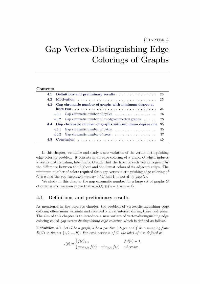
4 Gap Vertex-Distinguishing Edge Colorings of Graphs 23
4.1 Definitions and preliminary results . . . . . . . . . . . . . . . . . . . 23
4.2 Motivation . . . . . . . . . . . . . . . . . . . . . . . . . . . . . . . . . 25
4.3 Gap chromatic number of graphs with minimum degree at least two 26
4.3.1 Gap chromatic number of cycles . . . . . . . . . . . . . . . . 26
4.3.2 Gap chromatic number of m-edge-connected graphs . . . . . . 28
4.4 Gap chromatic number of graphs with minimum degree one . . . . . 35
4.4.1 Gap chromatic number of paths . . . . . . . . . . . . . . . . . 35
4.4.2 Gap chromatic number of trees . . . . . . . . . . . . . . . . . 37
4.5 Conclusion . . . . . . . . . . . . . . . . . . . . . . . . . . . . . . . . . 40
II Graph Packing Problem 43
5 Labeled Packing of Graphs 45
5.1 Packing and embedding of unlabeled graphs . . . . . . . . . . . . . . 45
5.1.1 Basic definitions . . . . . . . . . . . . . . . . . . . . . . . . . 45
5.1.2 Packing of graphs of small size in a complete graph . . . . . . 47
iv Contents
5.1.3 Packing graphs with bounded maximum degree and bounded
girth in a complete graph . . . . . . . . . . . . . . . . . . . . 49
5.1.4 Graph packing and permutation structure . . . . . . . . . . . 50
5.1.5 Our observations . . . . . . . . . . . . . . . . . . . . . . . . . 52
5.2 Labeled Packing Problem . . . . . . . . . . . . . . . . . . . . . . . . 52
5.2.1 Definitions and general results . . . . . . . . . . . . . . . . . 52
5.2.2 Labeled-packing of k copies of cycles with order at least 4k . 56
5.2.3 Labeled packing of k copies of cycles of order at most 4k − 1 62
5.2.4 Summary and concluding remarks . . . . . . . . . . . . . . . 65
5.3 Conclusion . . . . . . . . . . . . . . . . . . . . . . . . . . . . . . . . . 67
6 Labeled Embedding of Trees and (n, n− 2)-graphs 69
6.1 Labeled fixed-point-free embedding of graphs . . . . . . . . . . . . . 69
6.1.1 Labeled-embedding and labeled fixed-point-free embedding of
paths . . . . . . . . . . . . . . . . . . . . . . . . . . . . . . . 70
6.1.2 Labeled embedding of caterpillars . . . . . . . . . . . . . . . 73
6.2 Labeled embedding of trees . . . . . . . . . . . . . . . . . . . . . . . 78
6.3 Labeled embedding of (n, n− 2) graphs . . . . . . . . . . . . . . . . 84
6.4 Conclusion . . . . . . . . . . . . . . . . . . . . . . . . . . . . . . . . . 87
III XML Tree Pattern Matching Problem 89
7 Tree Matching and XML Retrieval 91
7.1 Querying XML Data: Key points . . . . . . . . . . . . . . . . . . . . 92
7.1.1 Tree representation of XML documents . . . . . . . . . . . . 92
7.1.2 Query languages . . . . . . . . . . . . . . . . . . . . . . . . . 94
7.2 Algorithms for exact tree pattern matching . . . . . . . . . . . . . . 96
7.2.1 Notation and terminology . . . . . . . . . . . . . . . . . . . . 96
7.2.2 Algorithms . . . . . . . . . . . . . . . . . . . . . . . . . . . . 96
7.3 Exact tree pattern matching for XML retrieval . . . . . . . . . . . . 98
7.3.1 Structural join approaches . . . . . . . . . . . . . . . . . . . . 98
7.3.2 Holistic twig join approaches . . . . . . . . . . . . . . . . . . 99
7.3.3 Sequence matching approaches . . . . . . . . . . . . . . . . . 102
7.3.4 Other important exact XML tree algorithms . . . . . . . . . . 103
7.3.5 Summary . . . . . . . . . . . . . . . . . . . . . . . . . . . . . 104
7.4 Conclusion . . . . . . . . . . . . . . . . . . . . . . . . . . . . . . . . . 104
8 TwigStack++: A New Efficient Holistic Twig Join Algorithm 107
8.1 Introduction . . . . . . . . . . . . . . . . . . . . . . . . . . . . . . . . 107
8.2 Containment labeling scheme of an XML document . . . . . . . . . . 108
8.3 Sub-optimality of TwigStack . . . . . . . . . . . . . . . . . . . . . . 109
8.4 A new algorithm: TwigStack++ . . . . . . . . . . . . . . . . . . . . 111
8.4.1 Notations . . . . . . . . . . . . . . . . . . . . . . . . . . . . . 111
8.4.2 TwigStack++ description . . . . . . . . . . . . . . . . . . . . 112

Contents v
8.5 Experimental result . . . . . . . . . . . . . . . . . . . . . . . . . . . . 118
8.6 Conclusion . . . . . . . . . . . . . . . . . . . . . . . . . . . . . . . . . 120
9 Conclusion and Future Work 121
Bibliography 125

List of Figures
2.1 Example of isomorphic graphs: f(u1) = v1, f(u2) = v3, f(u3) = v5,
f(u4) = v2 and f(u5) = v4. . . . . . . . . . . . . . . . . . . . . . . . 6
2.2 (a) G, (b) G. . . . . . . . . . . . . . . . . . . . . . . . . . . . . . . . 7
2.3 (a) Path graph, (b) Cycle graph. . . . . . . . . . . . . . . . . . . . . 8
2.4 Complete graphs (a) K1, (b) K2, (c) K3, (d) K4, (e) K5. . . . . . . . 8
2.5 Tree. . . . . . . . . . . . . . . . . . . . . . . . . . . . . . . . . . . . . 9
2.6 (a) Star graph, (b) Caterpillar. . . . . . . . . . . . . . . . . . . . . . 9
2.7 bipartite graph . . . . . . . . . . . . . . . . . . . . . . . . . . . . . . 9
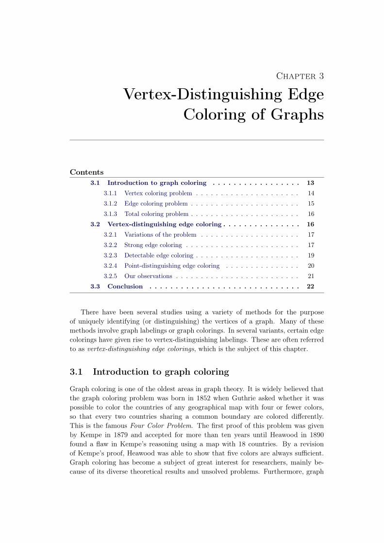
3.1 A graph with a proper 3-coloring . . . . . . . . . . . . . . . . . . . . 14
3.2 Coloring scheme of C7 for each variant in Tabel 3.1. . . . . . . . . . 19
4.1 A gap vertex-distinguishing edge coloring of a graph. . . . . . . . . . 24
4.2 A gap vertex-distinguishing edge coloring of Cn: (a) n = 8, (b) n = 9,
(c) n = 7, (d) n = 6. . . . . . . . . . . . . . . . . . . . . . . . . . . . 28
4.3 Illustration of Algorithm 1 (a=12): (a) A 2-edge-connected graph
G. (b) Coloring of R1. (c),(d),(e),(f) illustrates the coloring of
R2, R3, R4, R5, respectively. (g) A balanced gap-30-coloring of a span-
ning subgraph G′ of G. (h) A gap-30-coloring of G which induces a
gap vertex-distinguishing function l : V → {12, 13, . . . , 29}. . . . . . . 33
4.4 A gap-coloring of Pn: (a) n = 8, (b) n = 9, (c) n = 7, (d) n = 6. . . . 37
4.5 (a) Notation of BT3, (b) A gap-14-coloring of BT3 . . . . . . . . . . 38
4.6 Illustration of Algorithm 2: (a) A tree T . (b) Coloring of R1. (c),(d),(e),(f)
illustrates the coloring of R2, R3, R4, R5, respectively. (g) A gap-14-
coloring of T . . . . . . . . . . . . . . . . . . . . . . . . . . . . . . . . 39
5.1 A packing of two copies of P4 ∪ P3 into K7. . . . . . . . . . . . . . . 46
5.2 Example of a not 3-placeable tree . . . . . . . . . . . . . . . . . . . . 49
5.3 Five embeddable unicyclic graphs which are not cyclically embeddable. 51
5.4 A 5-labeled packing of two copies of P4 ∪ P3. . . . . . . . . . . . . . 52
5.5 (a) A caterpillar T , (b) A 10-labeled embedding of T . . . . . . . . 54
5.6 Proof structure. . . . . . . . . . . . . . . . . . . . . . . . . . . . . . . 56
5.7 Partition of V (C16) for k = 3. . . . . . . . . . . . . . . . . . . . . . . 57
5.8 A 10-labeled-packing of three copies of C16: (a) σ1(C16), (b) σ2(C16). 58
5.9 A 11-labeled-packing of three copies of C17: (a) σ1(C17), (b) σ2(C17). 59
5.10 A 9-labeled-packing of three copies of C15: (a) σ1(C15), (b) σ2(C15). 60
5.11 A 8-labeled-packing of three copies of C14: (a) σ1(C14), (b) σ2(C14). 61
5.12 A 7-labeled-embedding of C10 . . . . . . . . . . . . . . . . . . . . . 62
5.13 A 13-labeled-packing of three copies of C20: (a) σ1(C20), (b) σ2(C20). 63
5.14 A 7-labeled packing of three copies of C11: (a) σ1(C11), (b) σ2(C11). 64
viii List of Figures
5.15 A 3-labeled packing of three copies of C7: (a) σ1(C7), (b) σ2(C7). . . 66
5.16 A 4-labeled packing of three copies of C8: (a) σ1(C8), (b) σ2(C8). . . 67
6.1 A 3-labeled embedding of P5. . . . . . . . . . . . . . . . . . . . . . . 72
6.2 A 1-labeled embedding of P4. . . . . . . . . . . . . . . . . . . . . . . 72
6.3 Caterpillars with λ2(G) = |I|+ ⌊n−|I|2 ⌋ . . . . . . . . . . . . . . . . . 74
6.4 Caterpillars with λ2(G) = |I|+ ⌊n−|I|2 − 1⌋ . . . . . . . . . . . . . . 75
6.5 Caterpillars with λ2(G) = |I|+ ⌊n−|I|2 − 2⌋ . . . . . . . . . . . . . . . 75
6.6 A tree of diameter 4. . . . . . . . . . . . . . . . . . . . . . . . . . . . 79
6.7 Tree notation. . . . . . . . . . . . . . . . . . . . . . . . . . . . . . . . 80
6.8 Forbidden graphs . . . . . . . . . . . . . . . . . . . . . . . . . . . . . 81
6.9 A double star notation. . . . . . . . . . . . . . . . . . . . . . . . . . 83
6.10 Tu3 . . . . . . . . . . . . . . . . . . . . . . . . . . . . . . . . . . . . 83
6.11 Tx3. . . . . . . . . . . . . . . . . . . . . . . . . . . . . . . . . . . . . 85
7.1 An example of XML document . . . . . . . . . . . . . . . . . . . . . 93
7.2 XML tree associated with the document of Figure 7.1 . . . . . . . . 93
7.3 Example of a data-oriented document . . . . . . . . . . . . . . . . . 94
7.4 A twig query . . . . . . . . . . . . . . . . . . . . . . . . . . . . . . . 95
7.5 An example of tree pattern matching . . . . . . . . . . . . . . . . . . 97
8.1 A sample XML document with containment labels . . . . . . . . . . 108
8.2 (a) D: An XML data tree and (b) Q: A twig query pattern . . . . . 109
8.3 Illustrate to stack operations . . . . . . . . . . . . . . . . . . . . . . 110
8.4 (a) Tree pattern, (b) Structural star-path decomposition . . . . . . . 113
8.5 (a) D: An XML Data Tree and (b) Q: A Twig Query Pattern . . . . 117
8.6 Illustration to TwigStack++. . . . . . . . . . . . . . . . . . . . . . . 118
8.7 Running time of CPU and I/O on TreeBank . . . . . . . . . . . . . . 119
8.8 Running time of CPU and I/O on XMark . . . . . . . . . . . . . . . 120
List of Tables
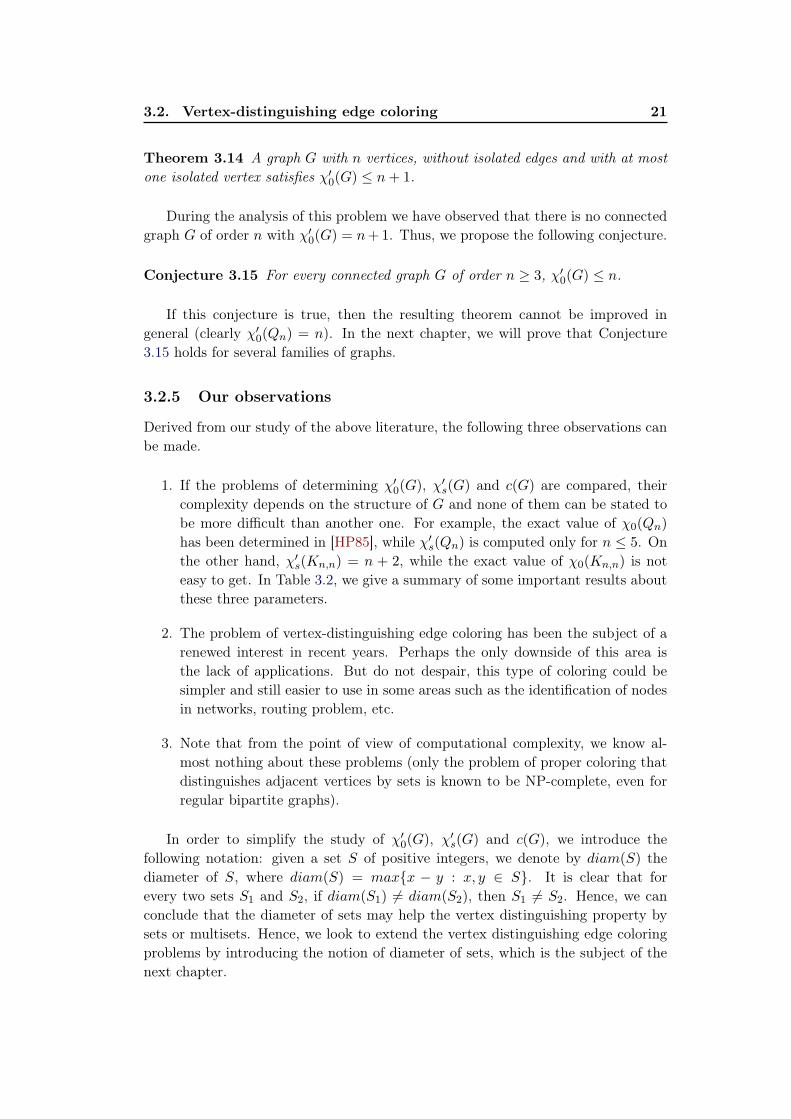
3.1 Summary of vertex distinguishing edge coloring of graphs . . . . . . 18
3.2 Summary of some important results about χ′s(G), c(G) and χ′
0(G). . 22
4.1 Our summary results on the gap chromatic number . . . . . . . . . . 41
7.1 Summary of XML retrieval approaches using XML exact tree matching105
8.1 Number of calls to getNext durning TwigStack . . . . . . . . . . . . 110
8.2 Queries used in our experiments . . . . . . . . . . . . . . . . . . . . . 119

Chapter 1
Introduction
Graph theory is an important field of mathematics and computer science. Originally,
it started in 1735 with the problem of the Seven Bridges of Königsberg. The city
of Königsberg in Prussia (modern Kaliningrad, Russia) was set on both sides of the
Pregel River, and included two islands connected to each other and the mainland
by seven bridges. The problem was to find a continuous tour through the city that
would cross each bridge exactly once, ending up at the point from which it began.
The Swiss mathematician, Leonard Euler, demonstrated that no such tour was pos-
sible. This result is often referred to as the first theorem in graph theory [Eul41].
Graphs are useful mathematical tools for modeling the relationships among objects,
which are represented by vertices. In their turn, relationships between vertices are
represented by edges. In this context, graph theory received considerable atten-
tion, not only from the mathematical community, but also from the whole scientific
community. Over the years, there have been a large number of significant and au-
thoritative publications in biochemistry, computer science, genetics or in sociology
where there is an interesting connection with graph theory.
These problems are most often modeled by finding an optimal structure in a
graph, generally a structure that must satisfy some constraints. For example, some
problems can be modeled by finding a maximum matching (i.e., a largest set of
edges without common vertices), a maximum stable set (i.e., a largest set of ver-
tices such that no two of them are linked by an edge), or a minimum coloring (i.e.,a minimum-cardinality partition of the vertices of a graph into stable sets).
Some problems can be solved efficiently, i.e., with a polynomial-time algorithm
(an algorithm is polynomial if its running time is bounded by a polynomial func-
tion according to the number and size of the inputs). For example, the problem of
computing a maximum matching can be solved using very efficient polynomial-time
algorithms. Unfortunately, many graph problems are hard in the sense that there
is (probably) no polynomial algorithm which solves these problems. More formally,
these problems are proved to be NP-hard (this is the case for minimum coloring and
maximum stable set problem). Another class of problems concerns those that have
not been classified yet as either polynomial or NP-hard. Isomorphism between two
graphs is one of the very few natural problems in this class. We say that two graphs
are isomorphic if there exists a permutation of the vertices that makes both graphs
identical.
2 Chapter 1. Introduction
Recently, graph theoretical concepts were widely used to study and model various
computer applications such as image segmentation, information retrieval, network-
ing, clustering, etc. For example in XML information retrieval, XML document
and query data can be represented by a graph model, and hence, retrieving XML
documents can be considered as a graph matching problem between the query tree
and the document trees (i.e., document/query isomorphism).
The three major problems considered in this thesis are the graph coloring prob-lem, the graph packing problem and the tree pattern matching. The common point
between these three problems is that they deal with labeled graphs. We thus di-
vided the thesis into three main parts, each containing two chapters, numbered from
3 to 8, where Chapter two is devoted to some basic graph theory concepts and
preliminary definitions, that are needed for the understanding of the results exposed
in this document.
Part 1: Graph coloring problem
Born with the famous Four Color Problem in 1852, the field of graph coloring has
become one of the most popular areas of graph theory. Graph coloring problems
come in many varieties but in general they consist in partitioning the objects (ver-
tices, edges, faces, etc.) of a graph into different classes so that given constraints are
satisfied. In its basic form, graph coloring is a way of coloring the vertices of a given
graph such that adjacent vertices get different colors; this is called the proper vertexcoloring problem. Similarly, a proper edge coloring problem assigns a color to each
edge so that every two adjacent edges receive different colors. About forty years ago,
many researchers considered the problem of assigning colors to the edges of a graph
G such that any two vertices of G are uniquely identified either by sets, multisets
or sums of their incident colors. The literature about these variants is reviewed in
Chapter three. Chapter four is intended to define a new graph coloring param-
eter called the gap vertex distinguishing edge coloring number, that combines many
features of the previously introduced methods. It consists in an edge-coloring of
a graph G which induces a vertex distinguishing labeling of G such that the label
of each vertex is given by the difference between the highest and the lowest colors
of its adjacent edges. In particular, we will study this problem for various families
of graphs and we will also show how this new parameter is strongly correlated to
the vertex distinguishing problem by sets and multisets. As a consequence, we will
provide bounds on these two problems.
Part 2: Graph packing problem
Graphs G1, G2, . . . , Gk (on n vertices each) pack, if there exists an edge disjoint
placement of them into the complete graph Kn. This problem is a classical one
in graph theory and has been extensively studied since the early 70’s. However,
the majority of existing works focuses on unlabeled graphs. In Chapter five, we
3
introduce for the first time the packing problem for a vertex labeled graph. Roughly
speaking, it consists in a classical graph packing which preserves the labels of the
vertices. Then, we study the corresponding optimization parameter for k copies of
cycles. In Chapter six, we study the labeled packing of two copies of trees and of
all graphs of order n and size n− 2. As an application, we will show that this new
problem can be used to solve the matching problem between two labeled graphs.
Part 3: XML Tree Pattern Matching Problem
With the increasing number of available XML documents, numerous approaches for
retrieval have been proposed in the literature. They usually use the tree repre-
sentation of documents and queries to process them in an implicit or explicit way.
Although retrieving XML documents can be considered as a tree matching prob-
lem between the query tree and the document trees, we consider in this part the
matching problem from an exact point of view. In Chapter seven, we outline
and compare the various features of different tree pattern algorithms. Most of these
algorithms find twig pattern matching in two steps. In the first one, a query tree is
decomposed into a set of binary patterns or single paths and then search for matches
for these individual patterns/paths. Finally, these matches are stitched together to
form the answers to the twig query. In Chapter eight, we propose a novel holistic
twig join algorithm, called TwigStack++, which features two main improvements
in the decomposition and matching phase. The proposed solutions are shown to be
efficient and scalable, and should be helpful for the future research on efficient query
processing in a large XML database.
Finally, in chapter nine, we summarize the results presented in this thesis, and
we give some remarks and directions for further research.
List of publications arising from this thesis
International journals
1. M. A. Tahraoui and H. Kheddouci. TwigStack++. A New Efficient
Holistic Twig Join Algorithm, In International Journal of Information-
Interaction-Intelligence (I3) N:02, 2011.
2. M. A. Tahraoui, E. Duchêne and H. Kheddouci. Gap vertex-distinguishing
edge colorings of graphs, Discrete Mathematics Volume 312(20):3011-
3025. 2012.
International conferences
3. E. Duchêne, H. Kheddouci, R. J. Nowakowski and M. A. Tahraoui. La-
beled Embeddings of Graphs. In SIAM Conference on Discrete Mathe-
matics, Canada, 2012.
4 Chapter 1. Introduction
4. M. A. Tahraoui, E. Duchêne, H. Kheddouci and R. J. Nowakowski. La-
beled packing of Graphs. In the proceedings of BCC 2011 - 23rd British
Combinatorial Conference. University of Exeter, Exeter, UK, 2011.
5. M. A Tahraoui and H. Kheddouci. An evolutionary algorithm for the k-b-
coloring problem. In the proceedings of 3nd International Conference on
Metaheuristics and Nature Inspired Computing META’10, Hammamet,
Tunisia, 2010.
6. M. A Tahraoui, E. Duchêne and H. Kheddouci. Max-Min vertex dis-
tinguishing edge colorings of graphs. In the proceedings of 8th French
Combinatorial Conference, Orsay, France, 2010.
International Journal, accepted with minor revision
7. M. A. Tahraoui, K. P. Sauvagnat, L. Ning, C. Lattang, M. Boughanem
and H. Kheddouci. A survey on tree matching and XML retrieval, Com-
puter Science Review.
8. E. Duchêne, H. Kheddouci, R. J. Nowakowski and M. A. Tahraoui. La-
beled packing of graphs, Australasian Journal of Combinatorics.
Submitted papers
9. M. A. Tahraoui, E. Duchêne and H. Kheddouci. Labeled embedding of
trees, Submitted to Discrete Mathematics.
Chapter 2
Preliminaries
Contents
2.1 Basic notations . . . . . . . . . . . . . . . . . . . . . . . . . . . 5
2.2 Some graph operations . . . . . . . . . . . . . . . . . . . . . . 6
2.3 Some families of graphs . . . . . . . . . . . . . . . . . . . . . . 7
We assume the reader is familiar with basic concepts of graph theory and the-
oretical computer science. We will thus give a short overview of the terminology
used in this thesis. More background information can be found in [CZ05], [Har69]
and [Wes96].
2.1 Basic notations
Graph: a graph G = (V (G), E(G)) consists of two finite sets: V (G), the vertex setof G, which is a non-empty set of elements called vertices and E(G) ⊆ V (G)×V (G)
is called set of edges. The cardinality of the vertex set V (G) is called the order of G,
commonly denoted by |V (G)|. The cardinality of the edge set E(G) is the size of G,
denoted by |E(G)|. A graph of order n and size m is often called an (n,m)-graph.
Two distinct vertices u and v are adjacent (or neighbors) if there exists an edge
uv that connects them. An edge uv is said to be incident to the vertices u and v.
Two edges are adjacent if they are incident to a same vertex. A graph is simple if
there is at most one edge between every two vertices. In this document, unless it is
specified, the graphs which are considered will be finite simple graphs.
Degree and Neighborhood: the set of all neighbors of a vertex v in a graph G is
denoted by N(v). The number of neighbors of v is called the degree of v in G, de-
noted by d(v). If d(v) = 0, it means that v is not adjacent to any other vertex, then v
is called an isolated vertex. A vertex of degree one is called an endpoint or a pendantvertex or a leaf. The minimum degree of a graph G is δ(G) = min{d(v) : v ∈ V (G)}
and the maximum degree of a graph G is denoted by△(G) = max{d(v) : v ∈ V (G)}.
Independent sets and Cliques: an independent set of G is a subset of vertices
U ⊆ V , such that no two vertices in U are adjacent. An independent set is said
to be maximal if no independent set properly contains it. An independent set of
maximum cardinality is called a maximum independent set. A clique in a graph G
6 Chapter 2. Preliminaries
is a subset C of V (G) such that every two vertices in C are adjacent in G. The
clique number ω(G) is the order of a maximum clique of G.
Distance and Connectivity: a path in an undirected graph G is a sequence of
vertices (v1, v2, . . . , vk) such that each pair vi, vi+1 is an edge in E(G). A path is
called simple if all its vertices are distinct. A graph G is connected if there exists
a path between any two distinct vertices of G. Otherwise, the graph G is discon-
nected. The distance between two vertices u, v in G, denoted by dist(u, v), is the
minimum number of edges in a path connecting them. The diameter of G is the
maximum distance between any two vertices of G. A graph is k-edge-connected if
there are k edge-disjoint paths between each pair of vertices or, equivalently, no two
vertices can be separated by removing less than k edges.
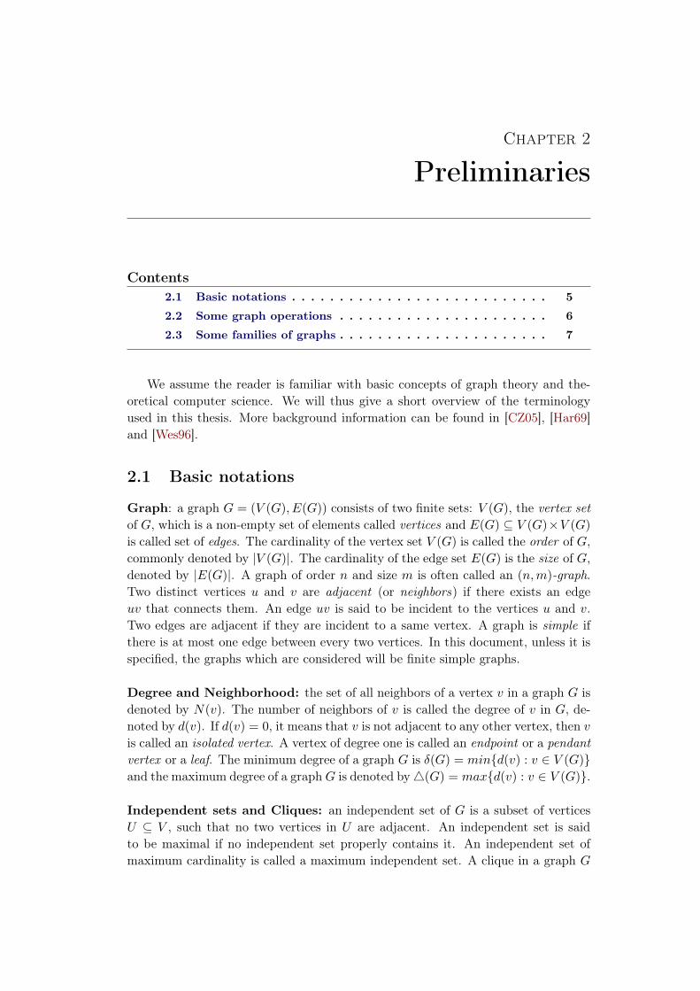
Isomorphism of graphs: two graphs G and H are said to be isomorphic (written
G ∼= H) if there is a one-to-one correspondence between their vertex-sets which
preserves the adjacency of vertices. We provide an example in Figure 2.1.
u4
u2
u3
u1
u5
(a)
v4
v2
v3
v1
v5
(b)
Figure 2.1: Example of isomorphic graphs: f(u1) = v1, f(u2) = v3, f(u3) = v5,
f(u4) = v2 and f(u5) = v4.
Subgraphs: a graph H is a subgraph of G, written H ⊆ G, if every vertex of H is a
vertex of G and every edge of H is an edge of G. In other words, V (H) ⊆ V (G) and
E(H) ⊆ E(G). We say that a subgraph H is a spanning subgraph, or a factor, of G
if H contains all the vertices of G. Given V ′ ⊆ V , the subgraph G[V ′] = (V ′, E′)
denotes the subgraph of G induced by V ′, i.e., E′ contains all the edges of E which
have both endpoints in V ′.
2.2 Some graph operations
In the following definitions, we detail some well known graph operations.
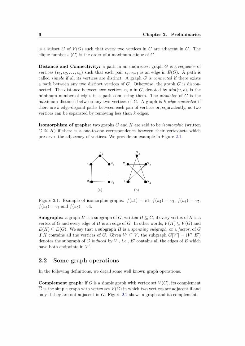
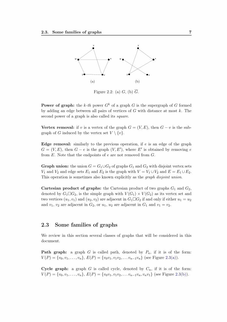
Complement graph: if G is a simple graph with vertex set V (G), its complement
G is the simple graph with vertex set V (G) in which two vertices are adjacent if and
only if they are not adjacent in G. Figure 2.2 shows a graph and its complement.
2.3. Some families of graphs 7
v
w x
y z
(a)
v
w x
y z
(b)
Figure 2.2: (a) G, (b) G.
Power of graph: the k-th power Gk of a graph G is the supergraph of G formed
by adding an edge between all pairs of vertices of G with distance at most k. The
second power of a graph is also called its square.
Vertex removal: if v is a vertex of the graph G = (V,E), then G − v is the sub-
graph of G induced by the vertex set V \ {v}.
Edge removal: similarly to the previous operation, if e is an edge of the graph
G = (V,E), then G − e is the graph (V,E′), where E′ is obtained by removing e
from E. Note that the endpoints of e are not removed from G.
Graph union: the union G = G1∪G2 of graphs G1 and G2 with disjoint vertex sets
V1 and V2 and edge sets E1 and E2 is the graph with V = V1∪V2 and E = E1∪E2.
This operation is sometimes also known explicitly as the graph disjoint union.
Cartesian product of graphs: the Cartesian product of two graphs G1 and G2,
denoted by G1�G2, is the simple graph with V (G1) × V (G2) as its vertex set and
two vertices (u1, v1) and (u2, v2) are adjacent in G1�G2 if and only if either u1 = u2and v1, v2 are adjacent in G2, or u1, u2 are adjacent in G1 and v1 = v2.
2.3 Some families of graphs
We review in this section several classes of graphs that will be considered in this
document.
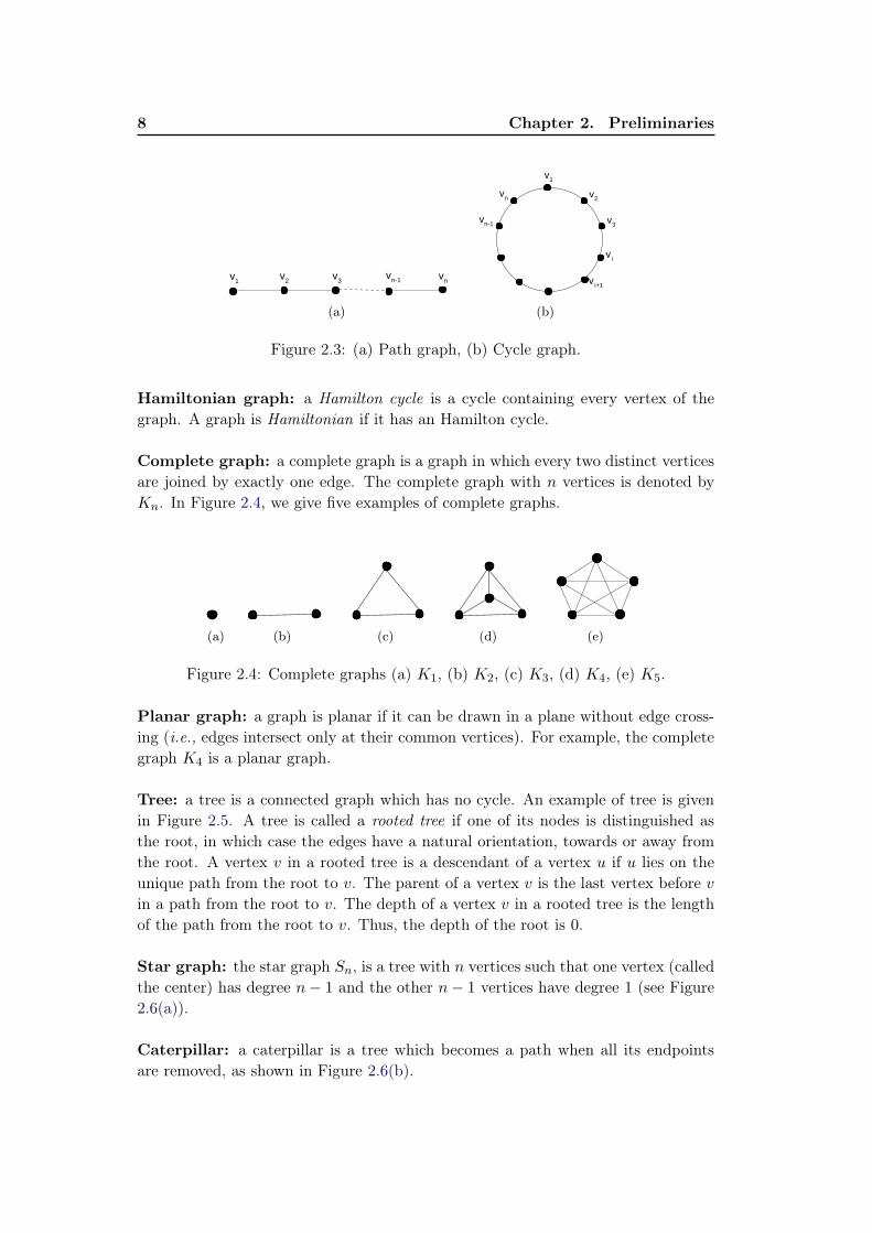
Path graph: a graph G is called path, denoted by Pn, if it is of the form:
V (P ) = {v0, v1, . . . , vn}, E(P ) = {v0v1, v1v2, . . . vn−1vn} (see Figure 2.3(a)).
Cycle graph: a graph G is called cycle, denoted by Cn, if it is of the form:
V (P ) = {v0, v1, . . . , vn}, E(P ) = {v0v1, v1v2, . . . vn−1vn, vnv1} (see Figure 2.3(b)).
8 Chapter 2. Preliminaries
v1 v2 v3vn-1 vn
(a)
v2
v3vn-1
vn
v1
v i
v i+1
(b)
Figure 2.3: (a) Path graph, (b) Cycle graph.
Hamiltonian graph: a Hamilton cycle is a cycle containing every vertex of the
graph. A graph is Hamiltonian if it has an Hamilton cycle.
Complete graph: a complete graph is a graph in which every two distinct vertices
are joined by exactly one edge. The complete graph with n vertices is denoted by
Kn. In Figure 2.4, we give five examples of complete graphs.
(a) (b) (c) (d) (e)
Figure 2.4: Complete graphs (a) K1, (b) K2, (c) K3, (d) K4, (e) K5.
Planar graph: a graph is planar if it can be drawn in a plane without edge cross-
ing (i.e., edges intersect only at their common vertices). For example, the complete
graph K4 is a planar graph.
Tree: a tree is a connected graph which has no cycle. An example of tree is given
in Figure 2.5. A tree is called a rooted tree if one of its nodes is distinguished as
the root, in which case the edges have a natural orientation, towards or away from
the root. A vertex v in a rooted tree is a descendant of a vertex u if u lies on the
unique path from the root to v. The parent of a vertex v is the last vertex before v
in a path from the root to v. The depth of a vertex v in a rooted tree is the length
of the path from the root to v. Thus, the depth of the root is 0.
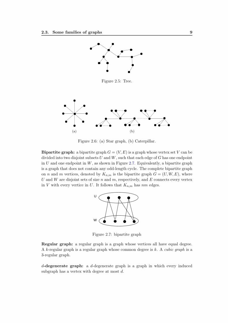
Star graph: the star graph Sn, is a tree with n vertices such that one vertex (called
the center) has degree n− 1 and the other n− 1 vertices have degree 1 (see Figure
2.6(a)).
Caterpillar: a caterpillar is a tree which becomes a path when all its endpoints
are removed, as shown in Figure 2.6(b).
2.3. Some families of graphs 9
Figure 2.5: Tree.
(a) (b)
Figure 2.6: (a) Star graph, (b) Caterpillar.
Bipartite graph: a bipartite graph G = (V,E) is a graph whose vertex set V can be
divided into two disjoint subsets U and W , such that each edge of G has one endpoint
in U and one endpoint in W , as shown in Figure 2.7. Equivalently, a bipartite graph
is a graph that does not contain any odd-length cycle. The complete bipartite graph
on n and m vertices, denoted by Kn,m is the bipartite graph G = (U,W,E), where
U and W are disjoint sets of size n and m, respectively, and E connects every vertex
in V with every vertice in U . It follows that Kn,m has nm edges.
U
W
Figure 2.7: bipartite graph
Regular graph: a regular graph is a graph whose vertices all have equal degree.
A k-regular graph is a regular graph whose common degree is k. A cubic graph is a
3-regular graph.
d-degenerate graph: a d-degenerate graph is a graph in which every induced
subgraph has a vertex with degree at most d.

Part I
Graph Coloring Problem

Chapter 3
Vertex-Distinguishing Edge
Coloring of Graphs
Contents
3.1 Introduction to graph coloring . . . . . . . . . . . . . . . . . 13
3.1.1 Vertex coloring problem . . . . . . . . . . . . . . . . . . . . . 14
3.1.2 Edge coloring problem . . . . . . . . . . . . . . . . . . . . . . 15
3.1.3 Total coloring problem . . . . . . . . . . . . . . . . . . . . . . 16
3.2 Vertex-distinguishing edge coloring . . . . . . . . . . . . . . . 16
3.2.1 Variations of the problem . . . . . . . . . . . . . . . . . . . . 17
3.2.2 Strong edge coloring . . . . . . . . . . . . . . . . . . . . . . . 17
3.2.3 Detectable edge coloring . . . . . . . . . . . . . . . . . . . . . 19
3.2.4 Point-distinguishing edge coloring . . . . . . . . . . . . . . . 20
3.2.5 Our observations . . . . . . . . . . . . . . . . . . . . . . . . . 21
3.3 Conclusion . . . . . . . . . . . . . . . . . . . . . . . . . . . . . 22
There have been several studies using a variety of methods for the purpose
of uniquely identifying (or distinguishing) the vertices of a graph. Many of these
methods involve graph labelings or graph colorings. In several variants, certain edge
colorings have given rise to vertex-distinguishing labelings. These are often referred
to as vertex-distinguishing edge colorings, which is the subject of this chapter.
3.1 Introduction to graph coloring
Graph coloring is one of the oldest areas in graph theory. It is widely believed that
the graph coloring problem was born in 1852 when Guthrie asked whether it was
possible to color the countries of any geographical map with four or fewer colors,
so that every two countries sharing a common boundary are colored differently.
This is the famous Four Color Problem. The first proof of this problem was given
by Kempe in 1879 and accepted for more than ten years until Heawood in 1890
found a flaw in Kempe’s reasoning using a map with 18 countries. By a revision
of Kempe’s proof, Heawood was able to show that five colors are always sufficient.
Graph coloring has become a subject of great interest for researchers, mainly be-
cause of its diverse theoretical results and unsolved problems. Furthermore, graph
14 Chapter 3. Vertex-Distinguishing Edge Coloring of Graphs
colorings have been proved to be paramount in other domains of graph theory (for
instance in the study of connectivity, matchings, Hamilton cycles) and also in real
world applications in many engineering fields, including register allocation [CH90],
timetabling [Wer85], frequency assignment [Gam86], scheduling [Lei79] and commu-
nication networks [WSW02].
3.1.1 Vertex coloring problem
Graph coloring problems that received the most attention deal with the vertices of
a graph. A proper vertex coloring of a graph G is a mapping f : V (G) −→ N (where
N is the set of positive integers) such that f(u) 6= f(v) if u and v are adjacent in G.
If f(V ) has size at most k, then we refer to the coloring as a k-coloring. A subset of
vertices assigned with the same color is called a color class, every such class being
an independent set. Thus, a k-coloring is equivalent to a partition of V (G) into k
independent sets, and the terms k-partite and k-colorable have the same meaning.
The following figure illustrates an example of a proper vertex coloring with three
colors.
1
3b
c
e
d g
f1
1
2
2
3
V ={a,e,g}1
V ={c,d}2
V={b,f}3
a
Figure 3.1: A graph with a proper 3-coloring
The chromatic number χ(G) of G is the minimum positive integer k for which
G has a k-coloring. Determining the chromatic number of a general graph G is
well-known to be a NP-hard problem [GJ79]. Consequently, much work has been
devoted to (1) determining bounds on the chromatic number of general graphs and
(2) determining the chromatic number of some families of graphs. It is quite easy to
see that for every graph G with maximum degree △(G), we have χ(G) ≤ △(G)+1.
However, Brooks has improved this bound as follows [Bro41].
Theorem 3.1 ([Bro41]) Let G be a connected graph. Then χ(G) ≤ △(G) unlessG is a complete graph or an odd cycle.
A rather obvious, but often useful, lower bound for the chromatic number of a
graph involves the chromatic numbers of its subgraphs.
Theorem 3.2 If H is a subgraph of a graph G, then χ(H) ≤ χ(G).
3.1. Introduction to graph coloring 15
The following result is an immediate consequence of the previous theorem.
Corollary 3.3 For every graph G, χ(G) ≥ ω(G).
A graph G is perfect if every induced subgraph H of G satisfies χ(H) = ω(H).
In the early 1960’s, Berge observed [Ber60, Ber61] that several classical families of
graphs (e.g. bipartite graphs, trees, interval graphs, chordal graphs) are perfect.
In [L7́2], the author showed that a complement of a perfect graph is also perfect.
However, there are also many graphs whose chromatic number exceeds their clique
number such as the Petersen graph and the odd cycles of length 5 or more. In
[GLS84], Grötschel et al. showed that the chromatic number of a perfect graph can
be determined in polynomial time. This is important as perfect graphs have many
connections to other combinatorial problems.
In addition to vertex coloring problems, many other types of graph coloring
problems have been formulated in the literature. However, the significance of vertex
coloring problems is often emphasized since many of these new problems can be
reformulated in terms of vertex colorings, or strongly depend on the chromatic
number. For more details on those variants, we refer the reader to the book of de
Werra and Hertz [WH89].
3.1.2 Edge coloring problem
After vertex colorings, it makes sense to study edge colorings. In this problem we
are looking for the minimum number of colors necessary to be assigned to the edges
of a graph such that any two incident edges are colored with different colors. This
parameter is called the chromatic index and is denoted by χ′(G). In 1965, Vizing
[Viz65] proved the famous Vizing’s theorem.
Theorem 3.4 ([Viz64]) For every nonempty graph G,
△(G) ≤ χ′(G) ≤ △(G) + 1
In [Hol81], Holyer proved that it is NP-complete to decide whether χ′(G) = △(G) or
χ′(G) = △(G) + 1. The chromatic index has been determined for several classes of
graphs. Indeed, bipartite graphs satisfy χ′(G) = △(G), while for odd cycles, we have
χ′(G) = △(G) + 1. For planar graphs, Vizing proposed the following conjecture:
Conjecture 3.5 ([Viz65]) For every planar graph G with maximum degree△(G) =
6 or 7, we haveχ′(G) = △(G)
This conjecture has been confirmed in [SZ01, Zha00] for △(G) = 7. But the case
△(G) = 6 remains an open problem.
Various generalizations of edge-coloring have been introduced and investigated
in the literature. In the 1970’s, Hilton and de Werra obtained many results on
equitable and edge-balanced colorings in which each color appears uniformly in G
16 Chapter 3. Vertex-Distinguishing Edge Coloring of Graphs
[HW82, Wer74, Wer75]. In the 1980’s Hakimi and Kariv [HK86] proposed the
following f -coloring problem: let f be a function which assigns a positive integer
f(v) to each vertex v ∈ V (G), an f -coloring of a graph G is a proper edge coloring
of G such that for each vertex v ∈ V , at most f(v) edges incident to v are colored
with the same color. The minimum number of colors needed to f -color G is called
the f -chromatic index χ′f (G) of G. Since the proper edge-coloring problem is NP-
complete, the f -coloring problem is also NP-complete in general. Various upper
bounds on χ′f (G) have been provided in [HK86, NNS88, Sey90].
3.1.3 Total coloring problem
We now consider colorings that assign colors to both vertices and edges of a graph.
A total coloring of a graph G is an assignment of colors to the vertices and edges of
G such that distinct colors are assigned to (i) every two adjacent vertices, (ii) every
two adjacent edges, and (iii) every incident vertex and edge. The total chromatic
number χ′′(G) of a graph G is the least number of colors needed in any total coloring
of G. Immediately, we have that χ′′(G) ≥ △(G) + 1. Sánchez-Arroyo [SA89] shown
that deciding whether a given graph has χ′′(G) = △(G) + 2 is an NP-complete
problem. The total coloring conjecture proposed independently by Behzad [Beh65]
and Vizing [Viz65] claims that for every simple graph G, χ′′(G) ≤ △(G) + 2. This
conjecture has been verified for a few important classes of graphs such as all bipartite
graphs and most planar graphs except those with maximum degree 6.
3.2 Vertex-distinguishing edge coloring
A problem in graph theory that has received considerable attention in the literature
concerns methods to uniquely identify the vertices of a connected graph. One of
the most popular methods is due to Entringer and Gassman [EG74] and Sumner
[Sum73]. They characterized the graphs G such that every two non-adjacent vertices
of G have distinct open neighborhoods. Harary and Melter [HM76] introduced the
idea of selecting a subset A = {u1, u2, . . . , uk} and labeling each vertex of v of G
with the ordered k-tuple l(v) = (d1, d2, . . . , dk) called distance label of v, where
di = dist(v, ui) for 1 ≤ i ≤ k. In this case, the vertices of G are distinguishable if
distinct vertices of G have distinct distance labels. The symmetry breaking method
was introduced by Harary [Har96, Har01] and, independently, by Albertson and
Collins [AC96]. In this method, the distinction of the vertices of G is realized with
the aid of a certain automorphism of G.
In this thesis, we are interested in another distinguishing method that is related
to the graph coloring problem. Indeed, many researchers investigated the question
of finding an edge coloring inducing a vertex distinguishing labeling. This is of-
ten referred to as vertex-distinguishing edge coloring. This problem has received
increasing attention in the literature during the past forty years. To the best of our
knowledge, four main different functions have been proposed to label each vertex v
3.2. Vertex-distinguishing edge coloring 17
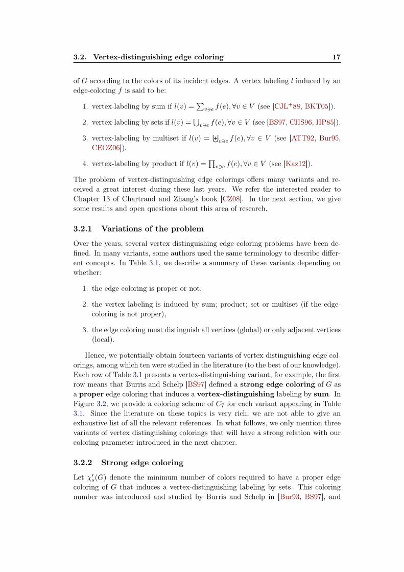
of G according to the colors of its incident edges. A vertex labeling l induced by an
edge-coloring f is said to be:
1. vertex-labeling by sum if l(v) =∑
v∋e f(e), ∀v ∈ V (see [CJL+88, BKT05]).
2. vertex-labeling by sets if l(v) =⋃
v∋e f(e), ∀v ∈ V (see [BS97, CHS96, HP85]).
3. vertex-labeling by multiset if l(v) =⊎
v∋e f(e), ∀v ∈ V (see [ATT92, Bur95,
CEOZ06]).
4. vertex-labeling by product if l(v) =∏
v∋e f(e), ∀v ∈ V (see [Kaz12]).
The problem of vertex-distinguishing edge colorings offers many variants and re-
ceived a great interest during these last years. We refer the interested reader to
Chapter 13 of Chartrand and Zhang’s book [CZ08]. In the next section, we give
some results and open questions about this area of research.
3.2.1 Variations of the problem
Over the years, several vertex distinguishing edge coloring problems have been de-
fined. In many variants, some authors used the same terminology to describe differ-
ent concepts. In Table 3.1, we describe a summary of these variants depending on
whether:
1. the edge coloring is proper or not,
2. the vertex labeling is induced by sum; product; set or multiset (if the edge-
coloring is not proper),
3. the edge coloring must distinguish all vertices (global) or only adjacent vertices
(local).
Hence, we potentially obtain fourteen variants of vertex distinguishing edge col-
orings, among which ten were studied in the literature (to the best of our knowledge).
Each row of Table 3.1 presents a vertex-distinguishing variant, for example, the first
row means that Burris and Schelp [BS97] defined a strong edge coloring of G as
a proper edge coloring that induces a vertex-distinguishing labeling by sum. In
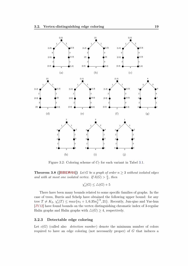
Figure 3.2, we provide a coloring scheme of C7 for each variant appearing in Table
3.1. Since the literature on these topics is very rich, we are not able to give an
exhaustive list of all the relevant references. In what follows, we only mention three
variants of vertex distinguishing colorings that will have a strong relation with our
coloring parameter introduced in the next chapter.
3.2.2 Strong edge coloring
Let χ′s(G) denote the minimum number of colors required to have a proper edge
coloring of G that induces a vertex-distinguishing labeling by sets. This coloring
number was introduced and studied by Burris and Schelp in [Bur93, BS97], and
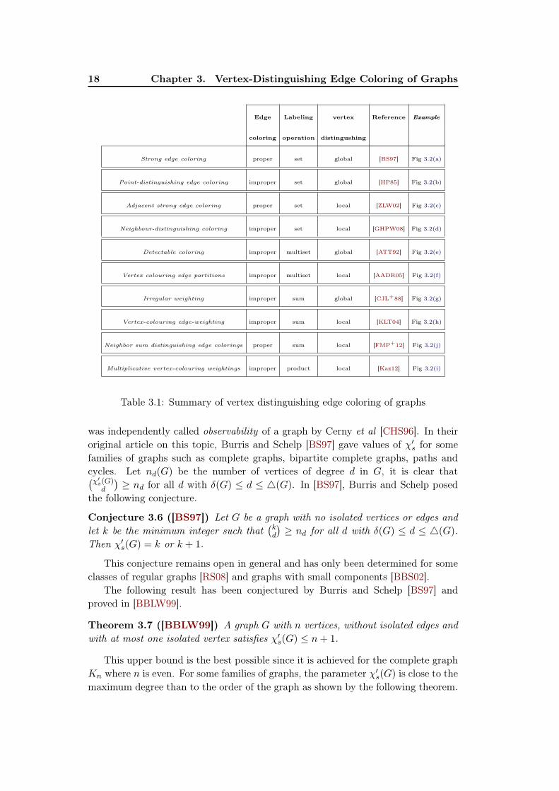
18 Chapter 3. Vertex-Distinguishing Edge Coloring of Graphs
Edge Labeling vertex Reference Example
coloring operation distingushing
Strong edge coloring proper set global [BS97] Fig 3.2(a)
Point-distinguishing edge coloring improper set global [HP85] Fig 3.2(b)
Adjacent strong edge coloring proper set local [ZLW02] Fig 3.2(c)
Neighbour-distinguishing coloring improper set local [GHPW08] Fig 3.2(d)
Detectable coloring improper multiset global [ATT92] Fig 3.2(e)
Vertex colouring edge partitions improper multiset local [AADR05] Fig 3.2(f)
Irregular weighting improper sum global [CJL+88] Fig 3.2(g)
Vertex-colouring edge-weighting improper sum local [KLT04] Fig 3.2(h)
Neighbor sum distinguishing edge colorings proper sum local [FMP+12] Fig 3.2(j)
Multiplicative vertex-colouring weightings improper product local [Kaz12] Fig 3.2(i)
Table 3.1: Summary of vertex distinguishing edge coloring of graphs
was independently called observability of a graph by Cerny et al [CHS96]. In their
original article on this topic, Burris and Schelp [BS97] gave values of χ′s for some
families of graphs such as complete graphs, bipartite complete graphs, paths and
cycles. Let nd(G) be the number of vertices of degree d in G, it is clear that(χ′
s(G)d
)
≥ nd for all d with δ(G) ≤ d ≤ △(G). In [BS97], Burris and Schelp posed
the following conjecture.
Conjecture 3.6 ([BS97]) Let G be a graph with no isolated vertices or edges andlet k be the minimum integer such that
(
kd
)
≥ nd for all d with δ(G) ≤ d ≤ △(G).Then χ′
s(G) = k or k + 1.
This conjecture remains open in general and has only been determined for some
classes of regular graphs [RS08] and graphs with small components [BBS02].
The following result has been conjectured by Burris and Schelp [BS97] and
proved in [BBLW99].
Theorem 3.7 ([BBLW99]) A graph G with n vertices, without isolated edges andwith at most one isolated vertex satisfies χ′
s(G) ≤ n+ 1.
This upper bound is the best possible since it is achieved for the complete graph
Kn where n is even. For some families of graphs, the parameter χ′s(G) is close to the
maximum degree than to the order of the graph as shown by the following theorem.
3.2. Vertex-distinguishing edge coloring 19
1
1
2
2
35
4
{2,5}
{1,5}
{1,2}
{2,3}
{1,3}
{1,4}{2,4}
(a)
1
3
1
2
32
4
{2}
{1,2}
{1}
{1,3}
{3}
{3,4}{2,4}
(b)
1
1
2
2
33
4
{2,3}
{1,3}
{1,2}
{2,3}
{1,3}
{1,4}{2,4}
(c)
1
2
1
3
22
3
{2,3}
{1,2}
{1}
{1,2}
{2}
{2,3}{3}
(d)
1
3
1
2
32
4
{2,2}
{1,2}
{1,1}
{1,3}
{3,3}
{3,4}{2,4}
(e)
1
3
1
2
33
2
{2,3}
{1,3}
{1,1}
{1,3}
{3,3}
{2,3}{2,2}
(f)
3
1
3
2
62
1
4
5
6
9
7
23
(g)
1
3
1
2
22
3
4
3
2
3
5
65
(h)
1
1
2
2
23
4
5
4
3
4
3
56
(i)
1
3
1
2
22
3
4
2
1
2
6
96
(j)
Figure 3.2: Coloring scheme of C7 for each variant in Tabel 3.1.
Theorem 3.8 ([BBLW01]) Let G be a graph of order n ≥ 3 without isolated edgesand with at most one isolated vertex. If δ(G) > n
3 , then
χ′s(G) ≤ △(G) + 5
There have been many bounds related to some specific families of graphs. In the
case of trees, Burris and Schelp have obtained the following upper bound: for any
tree T 6= K2, χ′s(T ) ≤ max{n1 + 1, 6.35n
1/22 , 21}. Recently, Jun-qiao and Yue-hua
[JY12] have found bounds on the vertex distinguishing chromatic index of 3-regular
Halin graphs and Halin graphs with △(G) ≥ 4, respectively.
3.2.3 Detectable edge coloring
Let c(G) (called also detection number) denote the minimum number of colors
required to have an edge coloring (not necessarily proper) of G that induces a
20 Chapter 3. Vertex-Distinguishing Edge Coloring of Graphs
vertex-distinguishing labeling by multisets. The following result has been stated
in [ATT92].
Theorem 3.9 ( [ATT92]) Let c be a k-coloring of the edges of a graph G. Themaximum number of different labels of the vertices of degree r in G is
(
r+k−1r
)
.
In other words, this means the following:
Corollary 3.10 If c is a detectable k-coloring of a connected graph G of order atleast 3, then G contains at most
(
r+k−1r
)
vertices.
Since vertices with distinct degrees in a connected graph always have distinct
labels, then, it seemed most challenging to study the graphs having many vertices
of the same degree. Indeed, the parameter c(G) of complete graphs and complete
bipartite graphs have been determined and detectable colorings of connected r-
regular graphs and trees have been studied as well (see [ATT92], [Bur94],[Bur95],
[CEOZ06]).
The detection number of cycles and paths have been determined in [CEOZ06]
and [EP05], respectively.
Theorem 3.11 ([CEOZ06]) Let n ≥ 3 be an integer and let l = ⌈√
n2 ⌉. Then
c(Cn) =
{
2l − 1 if 2(l − 1)2 + 1 ≤ n ≤ 2l2 − l
2l if 2l2 − l + 1 ≤ n ≤ 2l2
Theorem 3.12 ([EP05]) Let n ≥ 3 be an integer and let l = ⌈√
n2 ⌉. Then
c(Pn) =
{
2l if 2l2 − l + 1 ≤ n ≤ 2l2 + 3
2l + 1 if 2l2 + 4 ≤ n ≤ 2l2 + 3l + 2
The following result, stated in [CEOZ06], gives an upper bound for c(G) on a
connected graph.
Theorem 3.13 ([CEOZ06]) If G is a connected graph of order n ≥ 4, then c(G) ≤
n− 1.
This upper bound is obviously reached since there are many families of graphs
G with the property that c(G) = n− 1 such as K1,n for n ≥ 2, K3, K4, P3 and C4.
3.2.4 Point-distinguishing edge coloring
Let χ′0(G) denote the minimum number of colors required to have an edge coloring
(not necessarily proper) of a graph G that induces a vertex distinguishing labeling
by sets. Harary and Plantholt [HP85] referred to this type of coloring as the point-distinguishing edge coloring. They proved, among other things, the exact value of
χ′0(Pn), χ
′0(Cn), χ
′0(Qn) and χ′
0(Kn) for n ≥ 3. For bipartite graphs it seems that
the problem of determining χ′0(Km,n) is not easy (see [HS97, HS06, Sal90]).
Clearly we have c(G) ≤ χ′0(G) ≤ χ′
s(G), and the following result follows from
Theorem 3.7.
3.2. Vertex-distinguishing edge coloring 21
Theorem 3.14 A graph G with n vertices, without isolated edges and with at mostone isolated vertex satisfies χ′
0(G) ≤ n+ 1.
During the analysis of this problem we have observed that there is no connected
graph G of order n with χ′0(G) = n+1. Thus, we propose the following conjecture.
Conjecture 3.15 For every connected graph G of order n ≥ 3, χ′0(G) ≤ n.
If this conjecture is true, then the resulting theorem cannot be improved in
general (clearly χ′0(Qn) = n). In the next chapter, we will prove that Conjecture
3.15 holds for several families of graphs.
3.2.5 Our observations
Derived from our study of the above literature, the following three observations can
be made.
1. If the problems of determining χ′0(G), χ′
s(G) and c(G) are compared, their
complexity depends on the structure of G and none of them can be stated to
be more difficult than another one. For example, the exact value of χ0(Qn)
has been determined in [HP85], while χ′s(Qn) is computed only for n ≤ 5. On
the other hand, χ′s(Kn,n) = n + 2, while the exact value of χ0(Kn,n) is not
easy to get. In Table 3.2, we give a summary of some important results about
these three parameters.
2. The problem of vertex-distinguishing edge coloring has been the subject of a
renewed interest in recent years. Perhaps the only downside of this area is
the lack of applications. But do not despair, this type of coloring could be
simpler and still easier to use in some areas such as the identification of nodes
in networks, routing problem, etc.
3. Note that from the point of view of computational complexity, we know al-
most nothing about these problems (only the problem of proper coloring that
distinguishes adjacent vertices by sets is known to be NP-complete, even for
regular bipartite graphs).
In order to simplify the study of χ′0(G), χ′
s(G) and c(G), we introduce the
following notation: given a set S of positive integers, we denote by diam(S) the
diameter of S, where diam(S) = max{x − y : x, y ∈ S}. It is clear that for
every two sets S1 and S2, if diam(S1) 6= diam(S2), then S1 6= S2. Hence, we can
conclude that the diameter of sets may help the vertex distinguishing property by
sets or multisets. Hence, we look to extend the vertex distinguishing edge coloring
problems by introducing the notion of diameter of sets, which is the subject of the
next chapter.
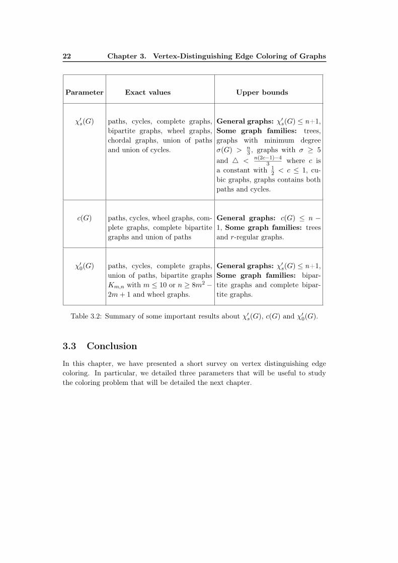
22 Chapter 3. Vertex-Distinguishing Edge Coloring of Graphs
Parameter Exact values Upper bounds
χ′s(G) paths, cycles, complete graphs,
bipartite graphs, wheel graphs,
chordal graphs, union of paths
and union of cycles.
General graphs: χ′s(G) ≤ n+1,
Some graph families: trees,
graphs with minimum degree
σ(G) > n3 , graphs with σ ≥ 5
and △ < n(2c−1)−43 where c is
a constant with 12 < c ≤ 1, cu-
bic graphs, graphs contains both
paths and cycles.
c(G) paths, cycles, wheel graphs, com-
plete graphs, complete bipartite
graphs and union of paths
General graphs: c(G) ≤ n −
1, Some graph families: trees
and r-regular graphs.
χ′0(G) paths, cycles, complete graphs,
union of paths, bipartite graphs
Km,n with m ≤ 10 or n ≥ 8m2 −
2m+ 1 and wheel graphs.
General graphs: χ′s(G) ≤ n+1,
Some graph families: bipar-
tite graphs and complete bipar-
tite graphs.
Table 3.2: Summary of some important results about χ′s(G), c(G) and χ′
0(G).
3.3 Conclusion
In this chapter, we have presented a short survey on vertex distinguishing edge
coloring. In particular, we detailed three parameters that will be useful to study
the coloring problem that will be detailed the next chapter.
Chapter 4
Gap Vertex-Distinguishing Edge
Colorings of Graphs
Contents
4.1 Definitions and preliminary results . . . . . . . . . . . . . . . 23
4.2 Motivation . . . . . . . . . . . . . . . . . . . . . . . . . . . . . 25
4.3 Gap chromatic number of graphs with minimum degree at
least two . . . . . . . . . . . . . . . . . . . . . . . . . . . . . . . 26
4.3.1 Gap chromatic number of cycles . . . . . . . . . . . . . . . . 26
4.3.2 Gap chromatic number of m-edge-connected graphs . . . . . 28
4.4 Gap chromatic number of graphs with minimum degree one 35
4.4.1 Gap chromatic number of paths . . . . . . . . . . . . . . . . . 35
4.4.2 Gap chromatic number of trees . . . . . . . . . . . . . . . . . 37
4.5 Conclusion . . . . . . . . . . . . . . . . . . . . . . . . . . . . . 40
In this chapter, we define and study a new variation of the vertex-distinguishing
edge coloring problem. It consists in an edge-coloring of a graph G which induces
a vertex distinguishing labeling of G such that the label of each vertex is given by
the difference between the highest and the lowest colors of its adjacent edges. The
minimum number of colors required for a gap vertex-distinguishing edge coloring of
G is called the gap chromatic number of G and is denoted by gap(G).
We study in this chapter the gap chromatic number for a large set of graphs G
of order n and we even prove that gap(G) ∈ {n− 1, n, n+ 1}.
4.1 Definitions and preliminary results
As mentioned in the previous chapter, the problem of vertex-distinguishing edge
coloring offers many variants and received a great interest during these last years.
The aim of this chapter is to introduce a new variant of vertex-distinguishing edge
coloring called gap vertex-distinguishing edge coloring, which is defined as follows:
Definition 4.1 Let G be a graph, k be a positive integer and f be a mapping fromE(G) to the set {1, 2, ..., k}. For each vertex v of G, the label of v is defined as
l(v) =
{
f(e)e∋v if d(v) = 1
maxe∋v f(e)−mine∋v f(e) otherwise
24 Chapter 4. Gap Vertex-Distinguishing Edge Colorings of Graphs
The mapping f is called a gap vertex-distinguishing edge coloring if distinct verticeshave distinct labels. Such a coloring is called a gap-k-coloring.
The minimum positive integer k for which G admits a gap-k-coloring is called the
gap chromatic number of G and is denoted by gap(G). Necessary and sufficient
conditions for the existence of such a coloring are given by the following proposition:
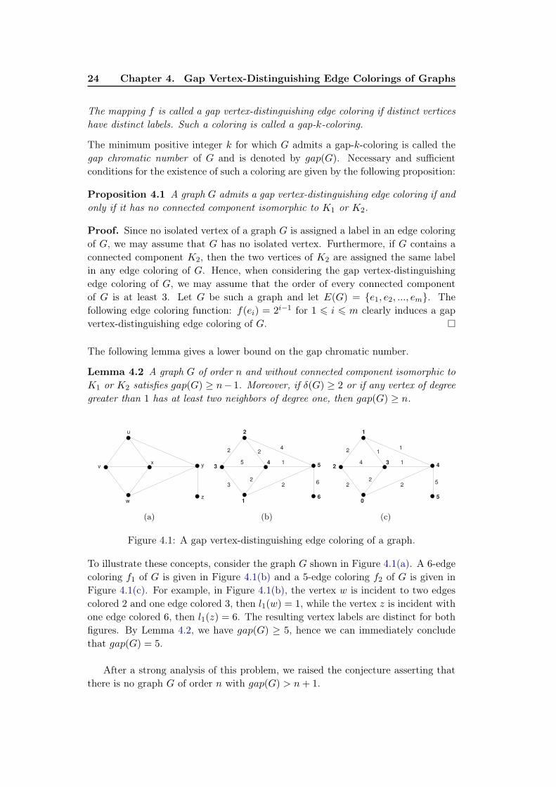
Proposition 4.1 A graph G admits a gap vertex-distinguishing edge coloring if andonly if it has no connected component isomorphic to K1 or K2.
Proof. Since no isolated vertex of a graph G is assigned a label in an edge coloring
of G, we may assume that G has no isolated vertex. Furthermore, if G contains a
connected component K2, then the two vertices of K2 are assigned the same label
in any edge coloring of G. Hence, when considering the gap vertex-distinguishing
edge coloring of G, we may assume that the order of every connected component
of G is at least 3. Let G be such a graph and let E(G) = {e1, e2, ..., em}. The
following edge coloring function: f(ei) = 2i−1 for 1 6 i 6 m clearly induces a gap
vertex-distinguishing edge coloring of G. �
The following lemma gives a lower bound on the gap chromatic number.
Lemma 4.2 A graph G of order n and without connected component isomorphic toK1 or K2 satisfies gap(G) ≥ n− 1. Moreover, if δ(G) ≥ 2 or if any vertex of degreegreater than 1 has at least two neighbors of degree one, then gap(G) ≥ n.
(a) (b) (c)
Figure 4.1: A gap vertex-distinguishing edge coloring of a graph.
To illustrate these concepts, consider the graph G shown in Figure 4.1(a). A 6-edge
coloring f1 of G is given in Figure 4.1(b) and a 5-edge coloring f2 of G is given in
Figure 4.1(c). For example, in Figure 4.1(b), the vertex w is incident to two edges
colored 2 and one edge colored 3, then l1(w) = 1, while the vertex z is incident with
one edge colored 6, then l1(z) = 6. The resulting vertex labels are distinct for both
figures. By Lemma 4.2, we have gap(G) ≥ 5, hence we can immediately conclude
that gap(G) = 5.
After a strong analysis of this problem, we raised the conjecture asserting that
there is no graph G of order n with gap(G) > n+ 1.
4.2. Motivation 25
Conjecture 4.3 For every connected graph G of order n ≥ 3, we have gap(G) ∈
{n− 1, n, n+ 1}.
In the following sections, we prove this conjecture for a large set of graphs and
we even decide the exact value of gap(G). The rest of this chapter is organized
as follows: first, we give in Section 4.2 some motivations to investigate this new
parameter. The results of Section 4.3 will confirm our conjecture for a large part
of graphs with minimum degree at least 2. In Section 4.4, we prove our conjecture
for some classes of graphs with minimum degree 1, such as paths, complete binary
trees and all trees with at least two leaves at distance 2. This classification of our
results according to δ(G) is due to the definition of our parameter, especially to the
definition of labels of vertices of degree one. Finally, concluding remarks are given
in the last section.
4.2 Motivation
In this section, we describe the motivation to study the gap coloring problem. First,
we give the following proposition, where we recall that the diameter of a set S,
denoted by diam(S) is the largest distance between any two points of the set.
Proposition 4.4 Let S1 and S2 be two sets of positive integers, if diam(S1) 6=
diam(S2), then S1 6= S2.
From the gap vertex labeling function (Definition 4.1), we observe that the label
of every vertex v with degree at least 2 is the diameter of the set of colors incident
to v. Note that this is not the case for the vertices of degree 1. Then, the gap
labeling of a graph G can be seen as a strong version of set and multisets label-
ings (defined in the previous chapter). Indeed, according to Proposition 4.4, a gap
distinguishing labeling of a graph G is also a multiset distinguishing labeling of G
and a set distinguishing labeling (if δ(G) > 1). Hence, we now characterize the
relationship between our coloring parameter and the two coloring parameters χ′0(G)
and c(G) defined previously. The following results follows from Proposition 4.4 and
the definitions of χ′0(G) and c(G).
Lemma 4.5 For every graph G without components isomorphic to either K1 or K2
and with minimum degree at least 2, we have
χ′0(G) ≤ gap(G)
Lemma 4.6 For every graph G, without components isomorphic to either K1 orK2, we have
c(G) ≤ gap(G)
We will see in Corollary 4.17 how the results of our parameter can be connected
to the study of χ′0(G).
26 Chapter 4. Gap Vertex-Distinguishing Edge Colorings of Graphs
4.3 Gap chromatic number of graphs with minimum de-
gree at least two
The main result of this section is the following:
Theorem 4.7 For every m-edge-connected graph G of order n with m ≥ 2,
gap(G) =
{
n if G is not a cycle of length ≡ 2, 3(mod 4)
n+ 1 otherwise
The proof of Theorem 4.7 is the combination of several results detailed below.
4.3.1 Gap chromatic number of cycles
Theorem 4.8 Let Cn be a cycle of order n, then
gap(Cn) =
{
n if n ≡ 0, 1(mod 4)
n+ 1 otherwise
Proof. Let Cn = (v1, v2, . . . , vn, vn+1 = v1). For each integer i with 1 ≤ i ≤ n, let
ei = vivi+1. We consider two cases as follows:
Case 1: n ≡ 0, 1(mod 4). By Lemma 4.2, we have gap(Cn) ≥ n, it then suffices to
prove that Cn admits a gap-n-coloring. Two subcases are considered:
Subcase 1.1: n ≡ 0(mod 4). A mapping f from E(Cn) to {1, 2, . . . , n} is defined
as follows (see Figure 4.2(a)).
For 1 ≤ i ≤ n, f(ei) =
n+ 1− i if i is odd
1 if i ≡ 2(mod 4)
2 if i ≡ 0(mod 4)
This mapping induces the following gap vertex labeling function:
For 1 ≤ i ≤ n, l(vi) =
n− i+ 1 if i ≡ 2(mod 4)
n− i if i ≡ 0, 3(mod 4)
n− i− 1 if i ≡ 1(mod 4)
Then, it is easy to check that l is a bijection from V (Cn) to {0, 1, . . . , n− 1}. Hence
gap(Cn) = n.
Subcase 1.2: n ≡ 1(mod 4). A mapping f from E(Cn) to {1, 2, . . . , n} is defined
as follows (see Figure 4.2(b)):
For 1 ≤ i ≤ n, f(ei) =
i if i is odd
n− 1 if i ≡ 2(mod 4)
n if i ≡ 0(mod 4)
4.3. Gap chromatic number of graphs with minimum degree at leasttwo 27
This mapping induces the following gap vertex labeling function:
For 1 ≤ i ≤ n, l(vi) =
n− i if i ≡ 1, 2(mod 4)
n− i+ 1 if i ≡ 0(mod 4)
n− i− 1 if i ≡ 3(mod 4)
Then, it is easy to check that l is a bijection from V (Cn) to {0, 1, . . . , n− 1}. Hence
gap(Cn) = n.
Case 2: n ≡ 2, 3(mod 4). We first prove that gap(Cn) > n. Let f : V (Cn) −→
{1, 2, . . . , n} be any edge-coloring of Cn which induces a gap vertex-distinguishing
function l. Now note that:
n∑
i=1
l(vi) =| f(e1)− f(en) | +n∑
i=2
| f(ei)− f(ei−1) |=n(n− 1)
2
In this formula, each term f(ei) appears twice with opposite (or same) signs, hencen(n−1)
2 is even. But this latter value is odd if n ≡ 2, 3(mod 4), which is a contradic-
tion. Thus, gap(Cn) ≥ n+ 1. It then remains to show that gap(Cn) ≤ n+ 1. Two
subcases are considered according to whether n mod 4 = 2 or 3.
Subcase 2.1: n ≡ 3(mod 4). We know that Cn+1 admits a gap-(n + 1)-coloring.
Necessarily, Cn+1 must contain two successive edges of same color j where 1 ≤ j ≤
n + 1. By merging these two edges into a single edge colored by j, we obtain a
gap-(n+ 1)-coloring of Cn (see Figure 4.2(c)).
Subcase 2.2: n ≡ 2(mod 4). In this subcase, we define an edge coloring f
from E(Cn) to {1, 2, . . . , n, n + 1} by (see Figure 4.2(d)) : f(en) = f(en−1) = 2,
f(en−2) = 3 and
For 1 ≤ i ≤ n− 3, f(ei) =
n+ 2− i if i is odd
1 if i ≡ 2(mod 4)
2 if i ≡ 0(mod 4)
This mapping induces the following gap vertex distinguishing labeling:
l(vn−2) = 2, l(vn−1) = 1, l(vn) = 0 and
For 1 ≤ i ≤ n− 3, l(vi) =
n− i if i ≡ 1(mod 4)
n+ 2− i if i ≡ 2(mod 4)
n+ 1− i if i ≡ 0, 3(mod 4)
Then, it is easy to check that l is a bijection from the vertex set of Cn to the set
{0, 1, . . . , n} \ {3}. Hence gap(Cn) = n+ 1. �
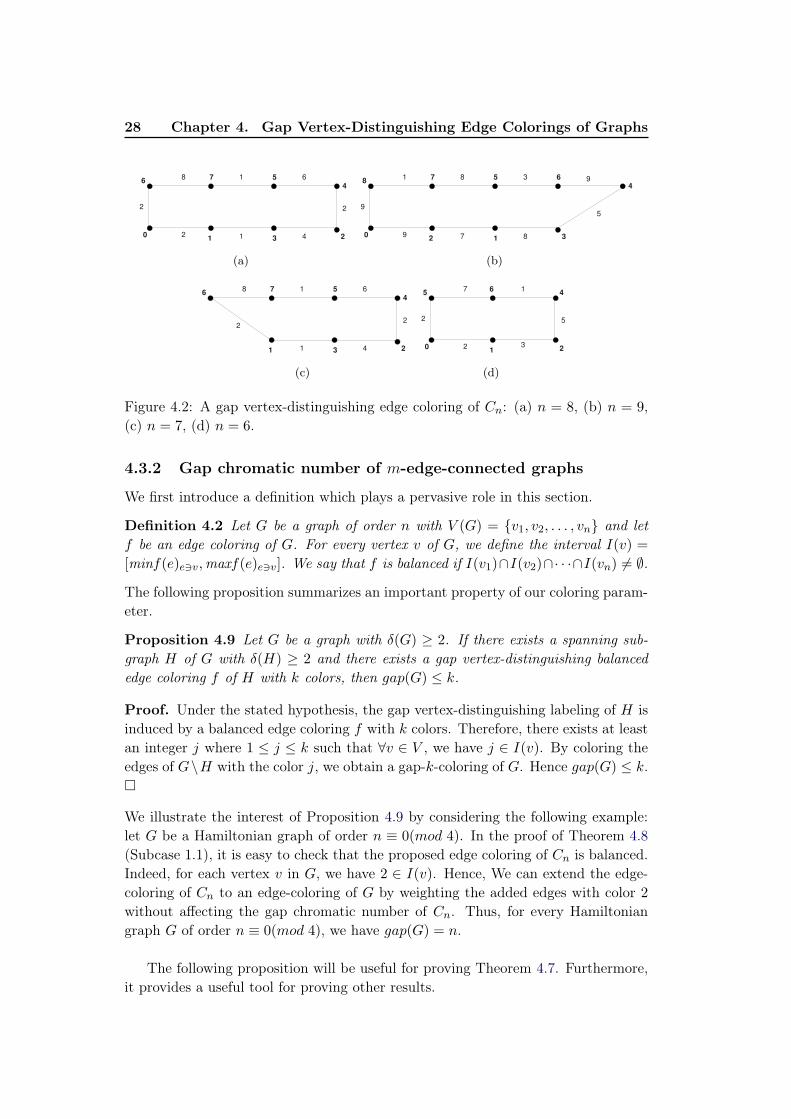
28 Chapter 4. Gap Vertex-Distinguishing Edge Colorings of Graphs
(a) (b)
(c) (d)
Figure 4.2: A gap vertex-distinguishing edge coloring of Cn: (a) n = 8, (b) n = 9,
(c) n = 7, (d) n = 6.
4.3.2 Gap chromatic number of m-edge-connected graphs
We first introduce a definition which plays a pervasive role in this section.
Definition 4.2 Let G be a graph of order n with V (G) = {v1, v2, . . . , vn} and letf be an edge coloring of G. For every vertex v of G, we define the interval I(v) =[minf(e)e∋v,maxf(e)e∋v]. We say that f is balanced if I(v1)∩I(v2)∩· · ·∩I(vn) 6= ∅.
The following proposition summarizes an important property of our coloring param-
eter.
Proposition 4.9 Let G be a graph with δ(G) ≥ 2. If there exists a spanning sub-graph H of G with δ(H) ≥ 2 and there exists a gap vertex-distinguishing balancededge coloring f of H with k colors, then gap(G) ≤ k.
Proof. Under the stated hypothesis, the gap vertex-distinguishing labeling of H is
induced by a balanced edge coloring f with k colors. Therefore, there exists at least
an integer j where 1 ≤ j ≤ k such that ∀v ∈ V , we have j ∈ I(v). By coloring the
edges of G\H with the color j, we obtain a gap-k-coloring of G. Hence gap(G) ≤ k.
�
We illustrate the interest of Proposition 4.9 by considering the following example:
let G be a Hamiltonian graph of order n ≡ 0(mod 4). In the proof of Theorem 4.8
(Subcase 1.1), it is easy to check that the proposed edge coloring of Cn is balanced.
Indeed, for each vertex v in G, we have 2 ∈ I(v). Hence, We can extend the edge-
coloring of Cn to an edge-coloring of G by weighting the added edges with color 2
without affecting the gap chromatic number of Cn. Thus, for every Hamiltonian
graph G of order n ≡ 0(mod 4), we have gap(G) = n.
The following proposition will be useful for proving Theorem 4.7. Furthermore,
it provides a useful tool for proving other results.
4.3. Gap chromatic number of graphs with minimum degree at leasttwo 29
Proposition 4.10 If G = (V,E) is an m-edge-connected graph of order n (withm ≥ 2), different from a cycle of length ≡ 1, 2 or 3(mod 4), then for every in-teger a ≥ 0, there exists an (a + n)-edge-coloring f which induces a gap vertex-distinguishing labeling l : V → {a, a+ 1, . . . , a+ n− 1}.
Proof. The proof of this proposition is done by giving a polynomial-time coloring
algorithm. Let us begin with some definitions and notations. For every subset S of
V , let NS denote the set of neighboring vertices of S, not included in S.
NS = {u ∈ V \ S : ∃v ∈ S for which (v, u) ∈ E}
For every two adjacent vertices u and v of G such that v ∈ S and u ∈ NS , let P (v, u)
be a function which returns a path (or cycle) from v to a vertex w ∈ S that passes
through u, such that the set of vertices between v and w does not belong to S.
Let f be an edge coloring of G. For every subgraph R of G, let g(R) be a function
defined on the set E(R) as follows:
g(R) = min{f(E(R) \ {1, 2}}
We denote by Q the set of all graphs that are isomorphic to a cycle of order multiple
of 4 or to two cycles having at least one vertex in common.
Observation Every m-edge-connected graph G (with m ≥ 2), different from a cycle
of length ≡ 1, 2 or 3(mod 4) contains at least one subgraph H ∈ Q.
It is clear that if G is a 2-edge-connected graph, different from a cycle, then
△(G) ≥ 3. Hence, the subgraph H can always be obtained from G. The basic idea
of our algorithm is to find a balanced (a+ n)-edge-coloring f of a 2-edge-connected
spanning subgraph G′ = (V ′, E′) of G. Initially, both sets V ′ and E′ are empty.
During the algorithm, the updating of V ′ and E′ is done gradually through a specific
edge coloring procedure (which is explained in more detail below). When an edge
of G is colored by this procedure it is inserted into E′. A vertex v ∈ V is inserted
into V ′ if and only if it is incident with at least two colored edges (e, s ∈ E′). Note
that when a vertex v is inserted in V ′, we set the label l(v) as l(v) = |f(e) − f(s)|
and the interval I(v) at [min(f(e), f(s)),max(f(e), f(s))]. Such an edge coloring
will ensure that for every interval I(v), we have 2 ∈ I(v).
In more details, the proposed algorithm starts by coloring the edges of a subgraph
H ∈ Q of G of order k which induces a gap vertex-distinguishing labeling of H, where
the vertices of H are labeled by distinct numbers ranging from n+a−k to n+a−1.
We can easily establish this labeling structure for every subgraph H of G which is
isomorphic to a member of Q. Then, we propose four edge-coloring functions to
color the set of edges which constructs a cycle that has an unique vertex in V ′ or
a path between two vertices of V ′. This last step is iterated until all vertices are
labeled (i.e., |V ′| = |V | ).

30 Chapter 4. Gap Vertex-Distinguishing Edge Colorings of Graphs
In order to color the subgraph H, we need to define several edge-coloring func-
tions. For a proper understanding of our algorithm, we are going to present the
algorithm for a graph G which contains at least one cycle of length multiple of
4. Otherwise, all other edge-coloring functions of H are described in detail in the
Appendix of [TDK12]. The different steps of the algorithm are illustrated in the
example of Figure 4.3, where a = 12.
Algorithm 1
Input: An integer a ≥ 0 and a m-edge-connected graph G = (V,E) of order n, such
that m ≥ 2 and G is not isomorphic to a cycle of length ≡ 1, 2 or 3(mod 4).
Output: A balanced (a + n)-edge-coloring f of G which induces a gap vertex-
distinguishing function l : V → {a, a+ 1, . . . , a+ n− 1}.
Begin of Algorithm
Step 1: V ′ ← ∅, E′ ← ∅. Let an index t = 2.
Step 2: Take any subgraph H = R1 ∈ Q of G.
2.1 If (R1 is a cycle of length k ≡ 0(mod 4)) Then
Let H = (v1, v2, . . . , vk, vk+1 = v1). For each integer i with 1 ≤ i ≤ k, let
ei = vivi+1. A mapping f from E(R1) to {1, 2, . . . , a+n} is defined as follows:
For 1 ≤ i ≤ k, f(ei) =
n+ a− i+ 1 if i is odd
1 if i ≡ 2(mod 4)
2 if i ≡ 0(mod 4)
This mapping induces the following vertex labeling of R1:
For 1 ≤ i ≤ k, l(vi) =
n+ a− i+ 1 if i ≡ 2(mod 4)
n+ a− i if i ≡ 0, 3(mod 4)
n+ a− i− 1 if i ≡ 1(mod 4)
Then, it is easy to check that l is a bijection from the vertex set of R1 to the
set {n+ a− 1, n+ a− 2, . . . , n+ a− k}.
Otherwise all other edge-coloring functions of R1 are described in detail in
the Appendix of [TDK12].
2.2 V ′ ← V (R1), E′ ← E(R1) and set z = g(R1).
Step 3: While ( V ′ 6= V ) do
Begin while
3.1 Take any two adjacent vertices u and v such that v ∈ V ′ and u ∈ NV ′ .
3.2 Let Rt = P (v, u), we represent the obtained subgraph Rt by the walk
(v1 = v, v2 = u, . . . , vk−1, vk). For each integer i with 1 ≤ i ≤ k − 1, let

4.3. Gap chromatic number of graphs with minimum degree at leasttwo 31
ei = vivi+1. We now define an edge coloring f of Rt. Four cases are considered
according to the value of k mod 4.
Case 1: k ≡ 0(mod 4). A mapping f from E(Rt) to {1, 2, . . . , a + n} is
defined as follows: f(ek−1) = z − k + 2 and
For 1 ≤ i ≤ k − 2, f(ei) =
z − i if i is odd
1 if i ≡ 0(mod 4)
2 if i ≡ 2(mod 4)
This mapping induces the following gap vertex labeling of Rt: l(vk−1) = z− k
and
For 2 ≤ i ≤ k − 2, l(vi) =
z − i− 1 if i ≡ 1, 2(mod 4)
z − i− 2 if i ≡ 3(mod 4)
z − i if i ≡ 0(mod 4)
Case 2: k ≡ 2(mod 4). A mapping f from E(Rt) to {1, 2, . . . , a + n} is
defined as follows:
For 1 ≤ i ≤ k − 1, f(ei) =
z − i if i is even
1 if i ≡ 3(mod 4)
2 if i ≡ 1(mod 4)
This mapping induces the following gap vertex labeling of Rt.
For 2 ≤ i ≤ k − 1, l(vi) =
z − i− 1 if i ≡ 0, 1(mod 4)
z − i− 2 if i ≡ 2(mod 4)
z − i if i ≡ 3(mod 4)
Case 3: k ≡ 1(mod 4). A mapping f from E(Rt) to {1, 2, . . . , a + n} is
defined as follows: f(e1) = z − 2 and
For 2 ≤ i ≤ k − 1, f(ei) =
z − i if i is odd
1 if i ≡ 2(mod 4)
2 if i ≡ 0(mod 4)
This mapping induces the following gap vertex labeling of Rt: l(v2) = z − 3
and
For 3 ≤ i ≤ k − 1, l(vi) =
z − i− 1 if i ≡ 0, 3(mod 4)
z − i− 2 if i ≡ 1(mod 4)
z − i if i ≡ 2(mod 4)
Case 4: k ≡ 3(mod 4). A mapping f from E(Rt) to {1, 2, . . . , a + n} is
defined as follows: f(ek−1) = z − k + 2 and
For 1 ≤ i ≤ k − 2, f(ei) =
z − i if i is even
1 if i ≡ 3(mod 4)
2 if i ≡ 1(mod 4)
32 Chapter 4. Gap Vertex-Distinguishing Edge Colorings of Graphs
This mapping induces the following gap vertex labeling of Rt: l(vk−1) = z−k,
and
For 2 ≤ i ≤ k − 2, l(vi) =
z − i− 1 if i ≡ 0, 1(mod 4)
z − i− 2 if i ≡ 2(mod 4)
z − i if i ≡ 3(mod 4)
Observation: In the previous four cases, it is easy to check that l is a bijec-
tion from the vertex set V (Rt)− {v1, vk} to {z − 3, z − 4, . . . , z − k}.
2.3 V ′ ← V ′ ∪ V (Rt), E′ ← E′ ∪ E(Rt). Set z = g(Rt) and t = t+ 1.
End while
Step 4: For all edges e ∈ E \ E′, set f(e) = 2.
End of algorithm.
We now present the proof of correctness of the above algorithm. We first show that
this algorithm achieves its goal without blocking, i.e., both actions in Step 3 (3.1
and 3.2) satisfy the following assertions:
If |V ′| < |V | then NV ′ 6= ∅. (4.1)
For every vertex u ∈ NV ′ there exists a path
from u to a vertex v ∈ V ′of order at least 2.(4.2)
The assertion (1) follows from the connectivity hypothesis on G. For a vertex
u ∈ NV ′ there exists, at last, an edge (u, v) ∈ E such that v ∈ V ′. The 2-edge-
connectivity hypothesis of G implies that every edge of G belongs to a cycle, then the
two vertices u and v belong to the same cycle. Therefore, the assertion (2) also holds.
We now prove that our coloring algorithm gives a gap vertex-distinguishing func-
tion l : V ′ → {a, a+ 1, . . . , a+ n− 1} of G′ induced by a balanced edge coloring f
with a + n colors. At the end of the loop of Step 3, we obtain a bijection l from
the set V ′ to the set {a, a+1, ..., a+ n− 1}, i.e., for any two vertices u, v of V ′, we
have l(u) 6= l(v). It then remains to show that f is a balanced edge-coloring and
for every vertex v of V ′, we have l(v) equal to maxe∋v f(e)−mine∋v f(e) in G′. By
considering the degree in G′ of each vertex v, we have two cases.
Case 1. d(v) = 2: from the algorithm, it is clear that the label of each vertex v of
degree 2 which is incident with two edges e and s of E′ is equal to |f(e)− f(s)|.
Case 2. d(v) > 2: let R(v) = {Rd1 , Rd2 , . . . , Rdp} denote the set of all subgraphs
having a common vertex v, where d1 ≤ d2 ≤ · · · ≤ dp. From the algorithm, we can
observe that (see Figure 4.3(g)):
• for any two subgraphs Ri and Rj of R(v), we have E(Ri) ∩ E(Rj) = ∅.
• v is incident with exactly two edges ed1 and sd1 of E(Rd1). Let f(ed1) ≥ f(sd1),
then the label of v is fixed as l(v) = f(ed1)− f(sd1).
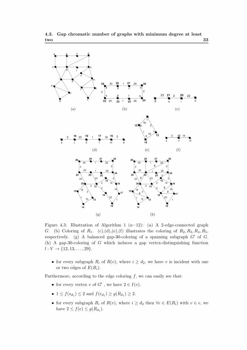
4.3. Gap chromatic number of graphs with minimum degree at leasttwo 33
(a) (b) (c)
(d) (e) (f)
(g) (h)
Figure 4.3: Illustration of Algorithm 1 (a=12): (a) A 2-edge-connected graph
G. (b) Coloring of R1. (c),(d),(e),(f) illustrates the coloring of R2, R3, R4, R5,
respectively. (g) A balanced gap-30-coloring of a spanning subgraph G′ of G.
(h) A gap-30-coloring of G which induces a gap vertex-distinguishing function
l : V → {12, 13, . . . , 29}.
• for every subgraph Ri of R(v), where i ≥ d2, we have v is incident with one
or two edges of E(Ri).
Furthermore, according to the edge coloring f , we can easily see that:
• for every vertex v of G′ , we have 2 ∈ I(v).
• 1 ≤ f(sd1) ≤ 2 and f(ed1) ≥ g(Rd1) ≥ 2.
• for every subgraph Ri of R(v), where i ≥ d2 then ∀e ∈ E(Ri) with v ∈ e, we
have 2 ≤ f(e) ≤ g(Rd1).
34 Chapter 4. Gap Vertex-Distinguishing Edge Colorings of Graphs
From these observations we can conclude the following:
• the edge-coloring f is balanced.
• for every vertex v of V ′, maxe∋v f(e) = f(ed1) and mine∋v f(e) = f(sd1).
At Step 4 of the algorithm, we know that the obtained edge coloring f of G′ is
balanced. Hence, we can extend G′ to G by coloring the added edges with color 2
without affecting the vertex labeling function l : V → {a, a+ 1, . . . , a+ n− 1}. �
Now, we can state the proof of Theorem 4.7. To proceed, we introduce the following
result.
Theorem 4.11 For every m-edge-connected graph G of order n (with m ≥ 2),different from a cycle of length n ≡ 2 or 3(mod 4), we have
gap(G) = n
Proof. By Lemma 4.2, we have gap(G) ≥ n. It then suffices to prove that G
admits a gap-n-coloring. We know by Theorem 4.8 that if G is a cycle of length
n ≡ 0, 1(mod 4), then gap(G) = n. Otherwise, it is clear by Proposition 4.10 that
if we set the integer parameter a at 0, we obtain a gap-n-coloring of G induced by
a balanced edge coloring. Hence gap(G) = n. �
We can now conclude that the result of Theorem 4.7 is a direct consequence of
Theorem 4.8 and Theorem 4.11.
Here we generalize the previous results to a special case of disconnected graphs as
follows:
Theorem 4.12 If G is a graph of order n with connected components G1, . . . , Gt,such that for every component Gi of G, Gi is different from a cycle of length ≡1, 2, 3(mod 4) and the edge connectivity of each component of G is at least 2, then
gap(G) = n
Proof. Let ni be the order of Gi (1 ≤ i ≤ t). The proof is essentially due to
Proposition 4.10. The idea is to provide a gap vertex distinguishing edge coloring for
each component of Gi according to the parameter a of Proposition 4.10 as follows: by
applying this proposition in sequence to G1, G2, . . . , Gt, we can obtain the labeling
function l : V (Gi) → {a, a + 1, . . . , a+ ni − 1} induced by an edge coloring f with
a + ni colors such that a = n −∑i
j=1 nj . From this, it is easy to check that l is a
bijection from the vertex set of G to the set {0, 1, 2, . . . , n− 1}. Thus gap(G) = n.
�
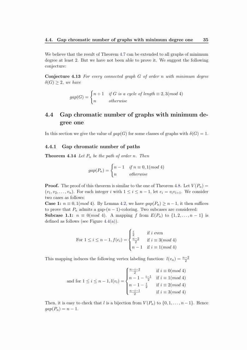
4.4. Gap chromatic number of graphs with minimum degree one 35
We believe that the result of Theorem 4.7 can be extended to all graphs of minimum
degree at least 2. But we have not been able to prove it. We suggest the following
conjecture:
Conjecture 4.13 For every connected graph G of order n with minimum degreeδ(G) ≥ 2, we have
gap(G) =
{
n+ 1 if G is a cycle of length ≡ 2, 3(mod 4)
n otherwise
4.4 Gap chromatic number of graphs with minimum de-
gree one
In this section we give the value of gap(G) for some classes of graphs with δ(G) = 1.
4.4.1 Gap chromatic number of paths
Theorem 4.14 Let Pn be the path of order n. Then
gap(Pn) =
{
n− 1 if n ≡ 0, 1(mod 4)
n otherwise
Proof. The proof of this theorem is similar to the one of Theorem 4.8. Let V (Pn) =
(v1, v2, . . . , vn). For each integer i with 1 ≤ i ≤ n− 1, let ei = vivi+1. We consider
two cases as follows:
Case 1: n ≡ 0, 1(mod 4). By Lemma 4.2, we have gap(Pn) ≥ n− 1, it then suffices
to prove that Pn admits a gap-(n− 1)-coloring. Two subcases are considered:
Subcase 1.1: n ≡ 0(mod 4). A mapping f from E(Pn) to {1, 2, . . . , n − 1} is
defined as follows (see Figure 4.4(a)).
For 1 ≤ i ≤ n− 1, f(ei) =
i2 if i evenn−22 if i ≡ 3(mod 4)
n− 1 if i ≡ 1(mod 4)
This mapping induces the following vertex labeling function: l(vn) =n−22
and for 1 ≤ i ≤ n− 1, l(vi) =
n−i−22 if i ≡ 0(mod 4)
n− 1− i−12 if i ≡ 1(mod 4)
n− 1− i2 if i ≡ 2(mod 4)
n−i−12 if i ≡ 3(mod 4)
Then, it is easy to check that l is a bijection from V (Pn) to {0, 1, . . . , n− 1}. Hence
gap(Pn) = n− 1.
36 Chapter 4. Gap Vertex-Distinguishing Edge Colorings of Graphs
Subcase 1.2: n ≡ 1(mod 4). A mapping f from E(Pn) to {1, 2, . . . , n − 1} is
defined as follows (see Figure 4.4(b)).
For 1 ≤ i ≤ n− 1, f(ei) =
i2 if i evenn−12 if i ≡ 3(mod 4)
n− 1 if i ≡ 1(mod 4)
This mapping induces the following vertex labeling function:
and for 1 ≤ i ≤ n− 1, l(vi) =
n−1−i2 if i ≡ 0(mod 4)
n− 1− i−12 if i ≡ 1(mod 4)
n− 1− i2 if i ≡ 2(mod 4)
n−i2 if i ≡ 3(mod 4)
Then, it is easy to check that l is a bijection from V (Pn) to {0, 1, . . . , n− 1}. Hence
gap(Pn) = n− 1.
Case 2: n ≡ 2, 3(mod 4). We first prove that gap(Pn) > n− 1. Let f : V (Pn) −→
{1, 2, . . . , n−1} be any edge-coloring of Pn which induces a gap vertex-distinguishing
labeling l. We note that:
n∑
i=1
l(vi) = f(e1) + f(en−1) +
n−1∑
i=2
| f(ei)− f(ei−1) |=n(n− 1)
2
In this formula, each term f(ei) appears twice with opposite (or same) signs, hencen(n−1)
2 is even. But this latter value is odd if n ≡ 2, 3(mod 4), which is a contradic-
tion. Thus, gap(Pn) ≥ n. It then remains to show that gap(Pn) ≤ n. Two subcases
are considered according to whether n mod 4 = 2 or 3.
Subcase 2.1: n ≡ 3(mod 4). We know that Pn+1 admits a gap-n-coloring. Neces-
sarily Pn+1 must contain two successive edges of same color j where 1 ≤ j ≤ n. By
merging these two edges into a single edge colored by j, we obtain a gap-n-coloring
of Pn (see Figure 4.4(c)).
Subcase 2.2: n ≡ 2(mod 4) In this subcase, we define an edge coloring f from
E(Pn) to {1, 2, . . . , n} (see Figure 4.4(d)) by f(en−1) = n− 1 and
For 1 ≤ i ≤ n− 2, f(ei) =
i2 + 1 if i evenn2 if i ≡ 3(mod 4)
n if i ≡ 1(mod 4)
This mapping induces the following gap vertex distinguishing labeling: l(v1) = n,
l(vn−1) =n2 − 1,l(vn) = n− 1 and
for 2 ≤ i ≤ n− 2, l(vi) =
n−i2 − 1 if i ≡ 0(mod 4)
n− i+12 if i ≡ 1(mod 4)
n− i2 − 1 if i ≡ 2(mod 4)
n−i−12 if i ≡ 3(mod 4)
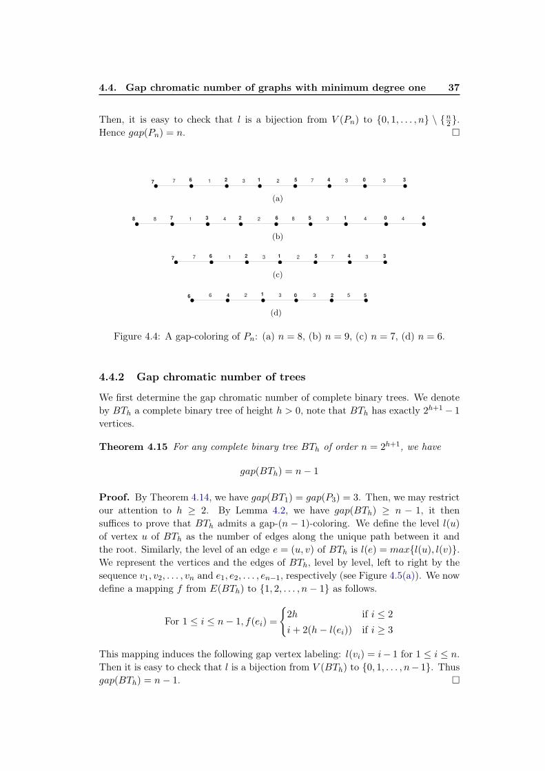
4.4. Gap chromatic number of graphs with minimum degree one 37
Then, it is easy to check that l is a bijection from V (Pn) to {0, 1, . . . , n} \ {n2 }.
Hence gap(Pn) = n. �
(a)
(b)
(c)
(d)
Figure 4.4: A gap-coloring of Pn: (a) n = 8, (b) n = 9, (c) n = 7, (d) n = 6.
4.4.2 Gap chromatic number of trees
We first determine the gap chromatic number of complete binary trees. We denote
by BTh a complete binary tree of height h > 0, note that BTh has exactly 2h+1 − 1
vertices.
Theorem 4.15 For any complete binary tree BTh of order n = 2h+1, we have
gap(BTh) = n− 1
Proof. By Theorem 4.14, we have gap(BT1) = gap(P3) = 3. Then, we may restrict
our attention to h ≥ 2. By Lemma 4.2, we have gap(BTh) ≥ n − 1, it then
suffices to prove that BTh admits a gap-(n − 1)-coloring. We define the level l(u)
of vertex u of BTh as the number of edges along the unique path between it and
the root. Similarly, the level of an edge e = (u, v) of BTh is l(e) = max{l(u), l(v)}.
We represent the vertices and the edges of BTh, level by level, left to right by the
sequence v1, v2, . . . , vn and e1, e2, . . . , en−1, respectively (see Figure 4.5(a)). We now
define a mapping f from E(BTh) to {1, 2, . . . , n− 1} as follows.
For 1 ≤ i ≤ n− 1, f(ei) =
{
2h if i ≤ 2
i+ 2(h− l(ei)) if i ≥ 3
This mapping induces the following gap vertex labeling: l(vi) = i− 1 for 1 ≤ i ≤ n.
Then it is easy to check that l is a bijection from V (BTh) to {0, 1, . . . , n− 1}. Thus
gap(BTh) = n− 1. �
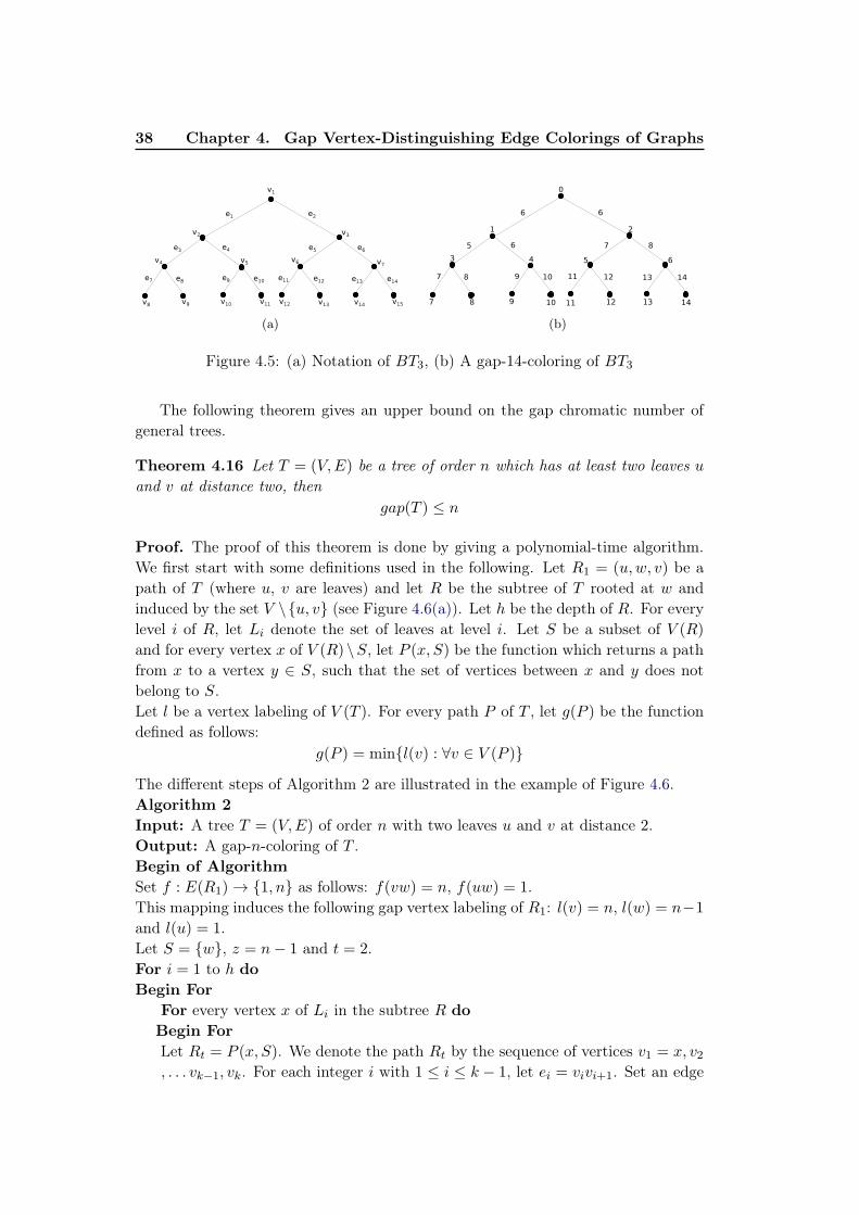
38 Chapter 4. Gap Vertex-Distinguishing Edge Colorings of Graphs
(a) (b)
Figure 4.5: (a) Notation of BT3, (b) A gap-14-coloring of BT3
The following theorem gives an upper bound on the gap chromatic number of
general trees.
Theorem 4.16 Let T = (V,E) be a tree of order n which has at least two leaves u
and v at distance two, thengap(T ) ≤ n
Proof. The proof of this theorem is done by giving a polynomial-time algorithm.
We first start with some definitions used in the following. Let R1 = (u,w, v) be a
path of T (where u, v are leaves) and let R be the subtree of T rooted at w and
induced by the set V \{u, v} (see Figure 4.6(a)). Let h be the depth of R. For every
level i of R, let Li denote the set of leaves at level i. Let S be a subset of V (R)
and for every vertex x of V (R) \S, let P (x, S) be the function which returns a path
from x to a vertex y ∈ S, such that the set of vertices between x and y does not
belong to S.
Let l be a vertex labeling of V (T ). For every path P of T , let g(P ) be the function
defined as follows:
g(P ) = min{l(v) : ∀v ∈ V (P )}
The different steps of Algorithm 2 are illustrated in the example of Figure 4.6.
Algorithm 2
Input: A tree T = (V,E) of order n with two leaves u and v at distance 2.
Output: A gap-n-coloring of T .
Begin of Algorithm
Set f : E(R1)→ {1, n} as follows: f(vw) = n, f(uw) = 1.
This mapping induces the following gap vertex labeling of R1: l(v) = n, l(w) = n−1
and l(u) = 1.
Let S = {w}, z = n− 1 and t = 2.
For i = 1 to h do
Begin For
For every vertex x of Li in the subtree R do
Begin For
Let Rt = P (x, S). We denote the path Rt by the sequence of vertices v1 = x, v2, . . . vk−1, vk. For each integer i with 1 ≤ i ≤ k − 1, let ei = vivi+1. Set an edge
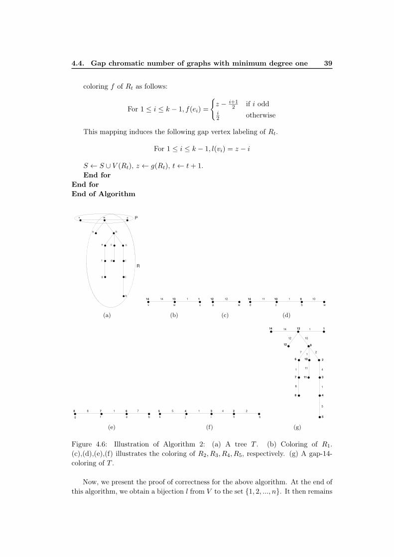
4.4. Gap chromatic number of graphs with minimum degree one 39
coloring f of Rt as follows:
For 1 ≤ i ≤ k − 1, f(ei) =
{
z − i+12 if i odd
i2 otherwise
This mapping induces the following gap vertex labeling of Rt.
For 1 ≤ i ≤ k − 1, l(vi) = z − i
S ← S ∪ V (Rt), z ← g(Rt), t← t+ 1.
End for
End for
End of Algorithm
(a) (b) (c) (d)
(e) (f) (g)
Figure 4.6: Illustration of Algorithm 2: (a) A tree T . (b) Coloring of R1.
(c),(d),(e),(f) illustrates the coloring of R2, R3, R4, R5, respectively. (g) A gap-14-
coloring of T .
Now, we present the proof of correctness for the above algorithm. At the end of
this algorithm, we obtain a bijection l from V to the set {1, 2, ..., n}. It then remains
40 Chapter 4. Gap Vertex-Distinguishing Edge Colorings of Graphs
to show the property of our coloring parameter. By considering the degree of each
vertex v of T , we have three cases:
Case 1. d(v) = 1: from the algorithm, it is clear that l(v) = f(e)e∋v.
Case 2. d(v) = 2: from the algorithm, it is clear that the label of vertex v of degree
2 which is incident with two edges e and s of E equals |f(e)− f(s)|.
Case 3. d(v) > 2: let R(v) = {Rd1 , Rd2 , . . . , Rdp} denote the set of all paths having
the vertex v in common, where d1 ≤ d2 ≤ · · · ≤ dp. We represent the distance
between two vertices x, y ∈ V by dist(x, y). From the algorithm, we can observe
that:
• every path Ri of R(v) contains a leaf li of T which is an endpoint of Ri. We
can see that dist(v, ld1) ≤ dist(v, ld2) ≤ · · · ≤ dist(v, ldp).
• for any two paths Ri and Rj of R(v), E(Ri) ∩ E(Rj) = ∅.
• the vertex v is incident with exactly two edges ed1 and sd1 of E(Rd1). Let
f(ed1) ≥ f(sd1), then the label of v is fixed as l(v) = f(ed1)− f(sd1).
• for every path Ri of R(v), where i ≥ d2, the vertex v is incident to exactly
one edge ei of E(Ri).
Furthermore, according to the edge-coloring f , we can see that:
• f(sd1) = ⌈dist(v,ld1 )
2 ⌉.
• for every path Ri of R(v), where i ≥ d2, we consider two cases for the value
of f(ei) (with v ∈ ei) according to the distance between v and li:
• dist(v, li) is even. We have f(ei) = dist(v,li)2 . Hence f(sd1) ≤ f(ei) ≤
g(Rd1) ≤ f(ed1).
• dist(v, li) is odd. We have f(ei) = g(Ri) +dist(v,li)−1
2 . Hence f(sd1) ≤
f(ei) ≤ g(Rd1) ≤ f(ed1).
From these observations, we can conclude that for every vertex v of V , f(ed1) =
maxe∋v f(e) and f(sd1) = mine∋v f(e). Hence, T admits a gap-n-coloring. �
4.5 Conclusion
In this chapter, we studied a new variant of graph edge coloring that induces a
vertex distinguishing labeling. Exact results are given for paths, cycles, some trees
and all m-edge-connected graphs with m ≥ 2. Our results are summarized in the
follwoing table.
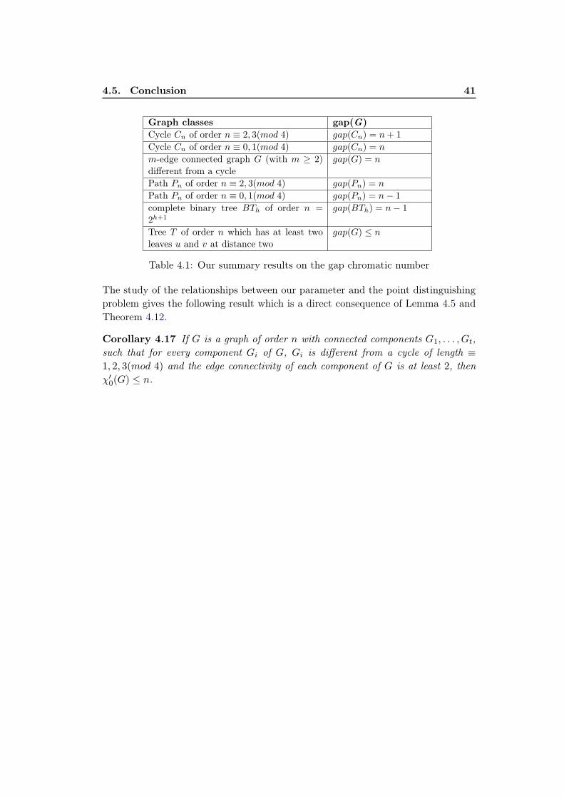
4.5. Conclusion 41
Graph classes gap(G)
Cycle Cn of order n ≡ 2, 3(mod 4) gap(Cn) = n+ 1
Cycle Cn of order n ≡ 0, 1(mod 4) gap(Cn) = n
m-edge connected graph G (with m ≥ 2)
different from a cycle
gap(G) = n
Path Pn of order n ≡ 2, 3(mod 4) gap(Pn) = n
Path Pn of order n ≡ 0, 1(mod 4) gap(Pn) = n− 1
complete binary tree BTh of order n =
2h+1
gap(BTh) = n− 1
Tree T of order n which has at least two
leaves u and v at distance two
gap(G) ≤ n
Table 4.1: Our summary results on the gap chromatic number
The study of the relationships between our parameter and the point distinguishing
problem gives the following result which is a direct consequence of Lemma 4.5 and
Theorem 4.12.
Corollary 4.17 If G is a graph of order n with connected components G1, . . . , Gt,such that for every component Gi of G, Gi is different from a cycle of length ≡1, 2, 3(mod 4) and the edge connectivity of each component of G is at least 2, thenχ′0(G) ≤ n.

Part II
Graph Packing Problem

Chapter 5
Labeled Packing of Graphs
Contents
5.1 Packing and embedding of unlabeled graphs . . . . . . . . . 45
5.1.1 Basic definitions . . . . . . . . . . . . . . . . . . . . . . . . . 45
5.1.2 Packing of graphs of small size in a complete graph . . . . . . 47
5.1.3 Packing graphs with bounded maximum degree and bounded
girth in a complete graph . . . . . . . . . . . . . . . . . . . . 49
5.1.4 Graph packing and permutation structure . . . . . . . . . . 50
5.1.5 Our observations . . . . . . . . . . . . . . . . . . . . . . . . . 52
5.2 Labeled Packing Problem . . . . . . . . . . . . . . . . . . . . 52
5.2.1 Definitions and general results . . . . . . . . . . . . . . . . . 52
5.2.2 Labeled-packing of k copies of cycles with order at least 4k . 56
5.2.3 Labeled packing of k copies of cycles of order at most 4k − 1 62
5.2.4 Summary and concluding remarks . . . . . . . . . . . . . . . 65
5.3 Conclusion . . . . . . . . . . . . . . . . . . . . . . . . . . . . . 67
In this chapter, we focus on graph packing problems, which are a well-known
field of graph theory for over 30 years. We start in Section 5.1 by presenting a variety
of results, some quite recent, concerning the packing of unlabeled graphs. We then
discuss the relationship between the embedding of graphs and the structure of the
embedding permutations. In Section 5.2, we introduce and study a new variant of
the graph packing problem, called the labeled packing of graphs. In particular, we
present some results and conjectures about cycles.
5.1 Packing and embedding of unlabeled graphs
5.1.1 Basic definitions
We here consider only finite simple graphs and use standard terminology notation
from Chapter 2 except when indicated. We recall that if a graph G has order n and
size m, we say that G is an (n,m)-graph. For more brevity, we will call an unlabeled
graph simply a graph.
A permutation σ is an one-to-one mapping of a set S into itself. We say that
an element e of S is a fixed point of a given permutation σ if σ(e) = e. Then, a
permutation σ is called fixed-point-free if σ has no fixed point. Any permutation σ of
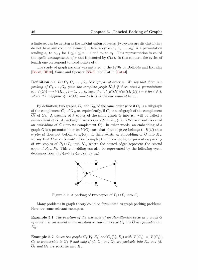
46 Chapter 5. Labeled Packing of Graphs
a finite set can be written as the disjoint union of cycles (two cycles are disjoint if they
do not have any common element). Here, a cycle (a1, a2, . . . , an) is a permutation
sending ai to ai+1 for 1 ≤ i ≤ n − 1 and an to a1. This representation is called
the cyclic decomposition of σ and is denoted by C(σ). In this context, the cycles of
length one correspond to fixed points of σ.
The study of graph packing was initiated in the 1970s by Bollobás and Eldridge
[Bol78, BE78], Sauer and Spencer [SS78], and Catlin [Cat74].
Definition 5.1 Let G1, G2, . . . , Gk be k graphs of order n. We say that there is apacking of G1, . . . , Gk (into the complete graph Kn) if there exist k permutationsσi : V (Gi) −→ V (Kn), i = 1, . . . , k, such that σ∗
i (E(Gi))∩σ∗j (E(Gj)) = ∅ for i 6= j,
where the mapping σ∗i : E(Gi) −→ E(Kn) is the one induced by σi.
By definition, two graphs, G1 and G2, of the same order pack if G1 is a subgraph
of the complement G2 of G2, or, equivalently, if G2 is a subgraph of the complement
G1 of G1. A packing of k copies of the same graph G into Kn will be called a
k-placement of G. A packing of two copies of G in Kn (i.e., a 2-placement) is called
an embedding of G (into its complement G). In other words, an embedding of a
graph G is a permutation σ on V (G) such that if an edge vu belongs to E(G) then
σ(v)σ(u) does not belong to E(G). If there exists an embedding of G into Kn,
we say that G is embeddable. For example, the following figure presents a packing
of two copies of P4 ∪ P3 into K7, where the dotted edges represent the second
copie of P4 ∪ P3. This embedding can also be represented by the following cyclic
decomposition: (x2)(x7)(x4)(x1, x6)(x3, x5).
x2
x3
x1
x4
x5
x6
x7
Figure 5.1: A packing of two copies of P4 ∪ P3 into K7.
Many problems in graph theory could be formulated as graph packing problems.
Here are some relevant examples.
Example 5.1 The question of the existence of an Hamiltonian cycle in a graph G
of order n is equivalent to the question whether the cycle Cn and G are packable intoKn.
Example 5.2 Given two graphs G1(V1, E1) and G2(V2, E2) with |V (G1)| = |V (G2)|,G1 is isomorphic to G2 if and only if (1) G1 and G2 are packable into Kn and (2)G1 and G2 are packable into Kn.
5.1. Packing and embedding of unlabeled graphs 47
Example 5.3 The independence number α(G) (α(G) represents the size of thelargest independent set of G) of a graph G of order n is at least p if and only ifG and the graph Kp ∪ (n− p)K1 (i.e., the graph consisting of the k-clique and n− p
isolated vertices) are packable into Kn.
In 1959, Erdős and Gallai [EG59] proved that every graph G with n vertices and
more than n(k−1)2 edges contains a path of length k. Motivated by this result, Erdős
and Sós made the following conjecture in 1963.
Conjecture 5.1 If G is a graph of order n and E(G) > n(k−1)2 , then G contains
every tree T of size k.
Example 5.4 We can easily see that if |E(G)| > n(k−1)2 then |E(G)| < n(n−k)
2 .Thus, Conjecture 5.1 can be formulated as follows: let G be a graph of order n andT any tree of order k, with k < n. If |E(G)| < n(n−k)
2 then there exists a packing ofG and T into Kn.
Packing of graphs is a heavily studied subject having many applications in com-
puter science (see e.g. [BE78, Haj91]). The reader can find a good survey on packing
of graphs in [Woz04] and [Yap88]. In general, the review of existing literature identi-
fies three different lines of research. The first one is about packing of general graphs
having small size in Kn(e.g. (n,m)-graphs with m ≤ n). The second one deals
with packing of graphs with bounded maximum degree and bounded girth in Kn.
The last one considers some additional properties of permutations in the packing
construction. We present in the following some important results in these areas.
5.1.2 Packing of graphs of small size in a complete graph
In 1978, Bollobás and Eldridge [BE78] made the following conjecture about the
existence of a k-packing of graphs of small size, which is generally considered to be
one of the most important open problems in graph packing theory.
Conjecture 5.2 ([BE78]) Let G1, G2 . . . Gk be k graphs of order n. If |E(Gi)| ≤
n− k, i = 1, 2, . . . k, then G1, G2, . . . Gk are packable into Kn.
So far only the cases k = 2 and k = 3 of this conjecture were proved in [SS78]
and [KMSW01], respectively. This shows the hardness of the problem and motivates
future research. In what follows, we survey some of the well known results relative
to the number of graphs to pack.
Packing of two graphs
The following theorem was independently proposed in [Bol78, BS77, SS78].
Theorem 5.3 ([Bol78, BS77, SS78]) Let G = (V,E) be a graph of order n. If|E(G)| ≤ n− 2 then G can be embedded in its complement.
48 Chapter 5. Labeled Packing of Graphs
The example of the star Sn shows that Theorem 5.3 cannot be improved by raising
the size of G even in the case when G is a tree. However, in this case we have the
following theorem, proved in [BS78], which completely characterizes the embedding
of (n, n− 1) graphs.
Theorem 5.4 ([BS78]) Let G = (V,E) be a graph of order n. If |E(G)| ≤ n − 1
then either G is embeddable in its complement or G is isomorphic to one of thefollowing graphs: K1,n−1,K1,n−4 ∪ K3 with n ≥ 8, K1 ∪ K3, K2 ∪ K3, K1 ∪ 2K3,K1 ∪ C4.
Among the exceptions mentioned in this theorem, the star K1,n−1 is the only
graph which is connected. Therefore, we have the following immediate consequence
(proved also in [HHS81]).
Theorem 5.5 ([HHS81]) Let T be a tree of order n, T 6= K1,n−1. Then T iscontained in its own complement.
These results has been improved in many ways. In Section 5.1.4, we are inter-
ested in improvements that deal with some additional properties of the permutation
structure.
Packing of three graphs
We are now going to consider the problem of packing of three graphs. We begin with
a theorem about the 3-placement of (n, n−2)-graphs, proved in [WW93], which can
be considered as an extension of Theorem 5.3.
Theorem 5.6 ([WW93]) Let G = (V,E) be a graph of order n. If |E(G)| ≤ n−2
then either there exists a 3-placement of G or G is isomorphic to K3 ∪ 2K1 or toK4 ∪ 4K1.
The following theorem refines Theorem 5.6 by specifying the permutation struc-
ture of the 3-placement of G (see [Woz94]).
Theorem 5.7 ([Woz94]) Let G = (V,E) be a graph of order n, G 6= K3 ∪
2K1,K4 ∪ 4K1. If |E(G)| ≤ n− 2, then there exists a permutation σ on V (G) suchthat σ1, σ2, σ3 define a 3-placement of G. Moreover, all cycles of σ have length 3,except for 1 of length one if n ≡ 1(mod 3) or two of length 1 if n ≡ 2(mod 3).
Now, consider the packing of three copies of a tree. Obviously, if there is a
packing of three copies of T into Kn, then we have
3(n− 1) ≤n(n− 1)
2
which implies n ≥ 6. Furthermore, since every vertex v of T with degree d(v) =
△(T ) must be mapped with two other vertices with degree at least one, then, we
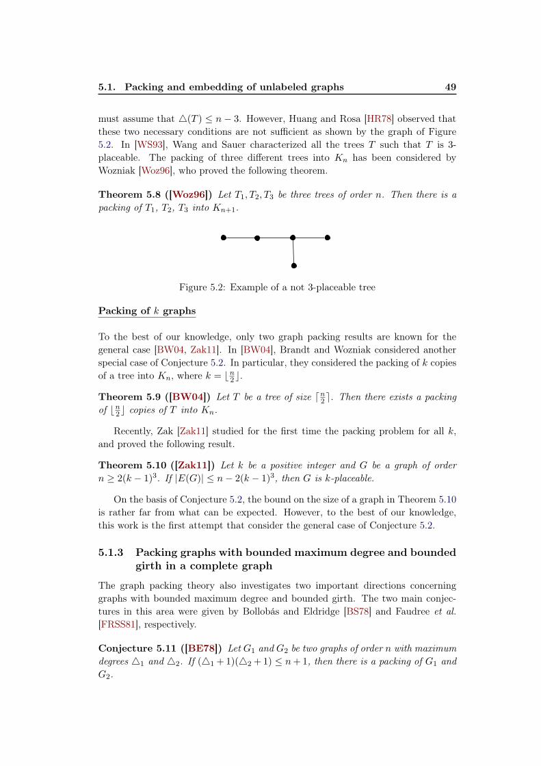
5.1. Packing and embedding of unlabeled graphs 49
must assume that △(T ) ≤ n− 3. However, Huang and Rosa [HR78] observed that
these two necessary conditions are not sufficient as shown by the graph of Figure
5.2. In [WS93], Wang and Sauer characterized all the trees T such that T is 3-
placeable. The packing of three different trees into Kn has been considered by
Wozniak [Woz96], who proved the following theorem.
Theorem 5.8 ([Woz96]) Let T1, T2, T3 be three trees of order n. Then there is apacking of T1, T2, T3 into Kn+1.
Figure 5.2: Example of a not 3-placeable tree
Packing of k graphs
To the best of our knowledge, only two graph packing results are known for the
general case [BW04, Zak11]. In [BW04], Brandt and Wozniak considered another
special case of Conjecture 5.2. In particular, they considered the packing of k copies
of a tree into Kn, where k = ⌊n2 ⌋.
Theorem 5.9 ([BW04]) Let T be a tree of size ⌈n2 ⌉. Then there exists a packingof ⌊n2 ⌋ copies of T into Kn.
Recently, Zak [Zak11] studied for the first time the packing problem for all k,
and proved the following result.
Theorem 5.10 ([Zak11]) Let k be a positive integer and G be a graph of ordern ≥ 2(k − 1)3. If |E(G)| ≤ n− 2(k − 1)3, then G is k-placeable.
On the basis of Conjecture 5.2, the bound on the size of a graph in Theorem 5.10
is rather far from what can be expected. However, to the best of our knowledge,
this work is the first attempt that consider the general case of Conjecture 5.2.
5.1.3 Packing graphs with bounded maximum degree and bounded
girth in a complete graph
The graph packing theory also investigates two important directions concerning
graphs with bounded maximum degree and bounded girth. The two main conjec-
tures in this area were given by Bollobás and Eldridge [BS78] and Faudree et al.[FRSS81], respectively.
Conjecture 5.11 ([BE78]) Let G1 and G2 be two graphs of order n with maximumdegrees △1 and △2. If (△1 +1)(△2 +1) ≤ n+1, then there is a packing of G1 andG2.
50 Chapter 5. Labeled Packing of Graphs
Conjecture 5.12 ([FRSS81]) If a graph G is a non-star graph without cycles oflength m ≤ 4, then G is embeddable.
If Conjecture 5.11 is true, then Conjecture 5.11 would be sharp, and considered
as an extension of the Hajnal-Szemerédi theorem [HS70] on equitable colorings. In-
deed, the Hajnal-Szemerédi theorem is a special case of Conjecture 5.11 when G2
is the disjoint union of cliques of the same size. This conjecture has been proved
in the case △1 ≤ 2 by Aigner and Brandt [AB93], and independently by Alon and
Fischer [AF96]. The case when △1 = 3 and n is huge has been proved by Csaba etal. in [CSS03]. Bollobás et al. [BKN08] proved a strengthening of the conjecture
when G1 is d-degenerate and d < △1
40 . Eaton [Eat00] showed that under the given
condition, there is a near-packing of degree 1 of G1 and G2, that is, an embedding
of the two graphs into a common vertex set such that the maximum degree of the
subgraph defined by the edges common to both copies is at most 1. Recently, Kaul
et al. [KKY08] proved Conjecture 5.11 for graphs with large maximum degrees.
They proved in particular that for △1,△2 ≥ 300, if (△1 + 1)(△2 + 1) ≤ 0.6n + 1,
then G1 and G2 pack.
In [FRSS81], Conjecture 5.12 was proved for every graph G with n vertices and
no more than 65n− 2 edges. Wozniak [Woz91] proved that a graph G without cycles
of length at most 7 is embeddable. This result was improved later by Brandt [Bur95]
who showed that a graph G without cycles of length at most 6 is embeddable. Re-
cently, Görlich and Zak [GZ09] proved that a graph G without cycles of length at
most 5 is embeddable.
5.1.4 Graph packing and permutation structure
In this section, we review some results concerning the relationship between the
embedding of graphs and the structure of the embedding permutations. This study
allows us to obtain some results concerning our graph packing problem which will
be introduced in Section 5.2. Let us start by the permutations with no fixed point.
In [Sch78], Schuster proved the following theorem.
Theorem 5.13 ([Sch78]) Let G = (V,E) be a graph of order n. If |E(G)| ≤ n−2
then there exists an embedding σ of G such that σ has no fixed point.
The above theorem cannot be improved by increasing the number of edges as shown
by the graphs K1,2∪K3 and K1,3∪K3. However, all the other (n, n−1)-graphs that
are contained in their complements can be embedded without fixed points. More
precisely, we have the following theorem (proved also in [Sch78]).
Theorem 5.14 ([Sch78]) Let G = (V,E) be a graph of order n with E(G) ≤ n−1.If (i) G is not an exceptional graph of Theorem 5.4 and (ii) G 6= K1,2 ∪ K3 andG 6= K1,3 ∪K3, then there exists a fixed-point-free embedding of G.

5.1. Packing and embedding of unlabeled graphs 51
Other work deal with the study of families of embeddable graphs such that the
corresponding permutation is cyclic. First of all, we formulate some results proved
in [Woz99] in the following theorem.
Theorem 5.15 ([Woz99]) The following graphs are cyclically embeddable:
1. non-star trees.
2. (n, n− 2) graphs.
3. cycles Cn for n ≥ 6.
4. unicyclic graphs, except graphs that are not embeddable at all (See [FRSS81])and five graphs given in Figure 5.3.
(a) (b) (c) (d) (e)
Figure 5.3: Five embeddable unicyclic graphs which are not cyclically embeddable.
Theorem 5.16 ([Woz99]) Let G be a graph of order n with |E(G)| ≤ n − 1 andsuch that (i) G is not an exceptional graph of Theorem 5.4 and (ii) G 6= K1,2 ∪
K3,K1,3 ∪K3,K1 ∪ C5. Then there exists a cyclic embedding of G.
Assume that an embedding σ of G is expressed as the product of disjoint cycles
(consedring σ as a permutation). The previous results can be improved in another
direction by specifying the size and the number of cycles occurring in the embedding
permutation. We begin with a theorem about embedding of (n, n−1)-graphs, proved
in [BW85], which can be considered as an improvement of Theorem 5.14.
Theorem 5.17 ([BW85]) Let G = (V,E) be a graph of order n, n ≡ 0, 1(mod4).If E(G) ≤ n − 1 then either there exists an embedding σ of G having all its cyclesof length 4, except for one of length 1 if n is odd, or G is isomorphic to one of thefollowing graphs: K1,n−1,K1,n−4 ∪K3, n ≥ 8, K1 ∪ C4, K1 ∪K3, K2 ∪K3.
The other cases (where n ≡ 2, 3(mod 4)) have been investigated by Wozniak in
[Woz94]. Another possibility for improvement of Theorem 5.13 is the following
theorem proved in [Woz94].
Theorem 5.18 ([Woz94]) Let G = (V,E) be a graph of order n, n ≥ 3. If|E(G)| ≤ n − 2 then there exists an embedding σ of G such that each cycle ofσ has length 3 except for one of length 1 if n ≡ 1(mod 3) or two of length 1 ifn ≡ 2(mod 3).
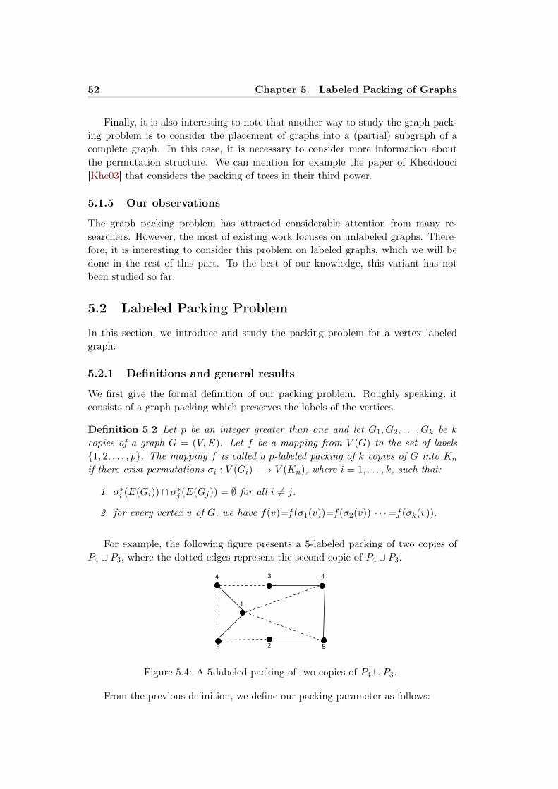
52 Chapter 5. Labeled Packing of Graphs
Finally, it is also interesting to note that another way to study the graph pack-
ing problem is to consider the placement of graphs into a (partial) subgraph of a
complete graph. In this case, it is necessary to consider more information about
the permutation structure. We can mention for example the paper of Kheddouci
[Khe03] that considers the packing of trees in their third power.
5.1.5 Our observations
The graph packing problem has attracted considerable attention from many re-
searchers. However, the most of existing work focuses on unlabeled graphs. There-
fore, it is interesting to consider this problem on labeled graphs, which we will be
done in the rest of this part. To the best of our knowledge, this variant has not
been studied so far.
5.2 Labeled Packing Problem
In this section, we introduce and study the packing problem for a vertex labeled
graph.
5.2.1 Definitions and general results
We first give the formal definition of our packing problem. Roughly speaking, it
consists of a graph packing which preserves the labels of the vertices.
Definition 5.2 Let p be an integer greater than one and let G1, G2, . . . , Gk be k
copies of a graph G = (V,E). Let f be a mapping from V (G) to the set of labels{1, 2, . . . , p}. The mapping f is called a p-labeled packing of k copies of G into Kn
if there exist permutations σi : V (Gi) −→ V (Kn), where i = 1, . . . , k, such that:
1. σ∗i (E(Gi)) ∩ σ∗
j (E(Gj)) = ∅ for all i 6= j.
2. for every vertex v of G, we have f(v)=f(σ1(v))=f(σ2(v)) · · ·=f(σk(v)).
For example, the following figure presents a 5-labeled packing of two copies of
P4 ∪ P3, where the dotted edges represent the second copie of P4 ∪ P3.
2
4 3
1
5
4
5
Figure 5.4: A 5-labeled packing of two copies of P4 ∪ P3.
From the previous definition, we define our packing parameter as follows:
5.2. Labeled Packing Problem 53
Definition 5.3 The maximum positive integer p for which G admits a p-labeledpacking of k copies of G is called the k-labeled packing number of G and is denotedby λk(G).
Naturally, the existence of a packing of k copies of a graph G is a necessary and
sufficient condition for the existence of a p-labeled packing of k copies of G (where
p ≥ 1). Indeed, it suffices to choose the mapping f : V (G) −→ {1}. Then, we
obtain the following proposition.
Proposition 5.19 For every graph G, if there exists a k-placement of G into Kn,then
λk(G) ≥ 1.
The following lemma is a direct consequence of Definition 5.2.
Lemma 5.20 Let G be a graph of order n and let H be a spanning subgraph of G.If there exists a packing of k copies of G into Kn, then
λk(H) ≥ λk(G).
Let us introduce the following notations: let G be a graph of order n and f be
a mapping from V (G) to {1, 2, . . . , p}. We define S(f) as the subset of labels that
occur only once in f(V (G)) and let VS(f) consist of the vertices colored with the
labels of S(f). Thus it is obvious that |VS(f)| = |S(f)|. Throughout this part, a
labeled packing of two copies of G will be called a labeled embedding of G.
The following lemma gives an upper bound on the labeled embedding number
λ2(G).
Lemma 5.21 Let G be a graph of order n and let I be a maximum independent setof G. If there exists an embedding of G, then
λ2(G) ≤ |I|+ ⌊n− |I|
2⌋
Proof. Let f be a mapping from V (G) to {1, 2 . . . , p} corresponding to a p-labeledembedding of G with p maximum, (i.e., p = λ2(G)). A necessary condition for the
existence of a p-labeled embedding of G is that for every two adjacent vertices of G,
one of their labels must occur at least twice in f(V (G)). Hence, it is easy to see
that all vertices of VS(f) form an independent set in G. Then, we have |VS(f)| ≤ |I|
and p ≤ |VS(f)|+ ⌊n−|VS(f)|
2 ⌋. Since g(x) = x+ ⌊n−x2 ⌋ is an increasing function of x,
it follows that p ≤ |I|+ ⌊n−|I|2 ⌋, giving the desired result. �
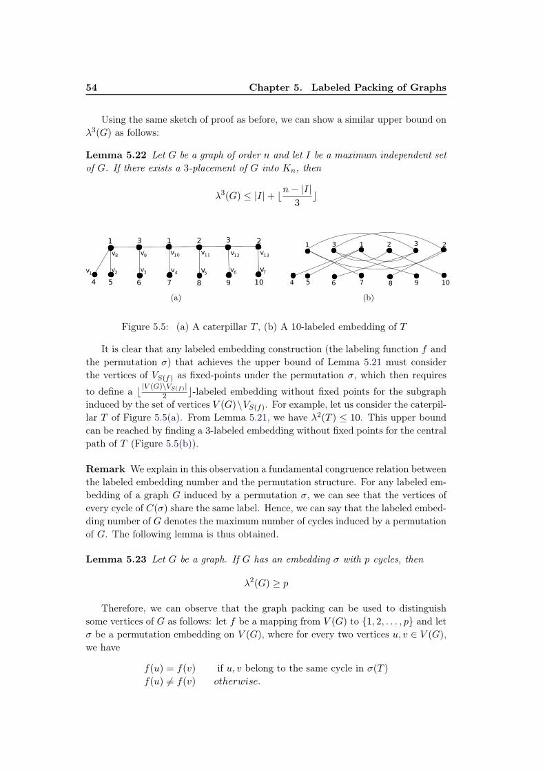
54 Chapter 5. Labeled Packing of Graphs
Using the same sketch of proof as before, we can show a similar upper bound on
λ3(G) as follows:
Lemma 5.22 Let G be a graph of order n and let I be a maximum independent setof G. If there exists a 3-placement of G into Kn, then
λ3(G) ≤ |I|+ ⌊n− |I|
3⌋
(a) (b)
Figure 5.5: (a) A caterpillar T , (b) A 10-labeled embedding of T
It is clear that any labeled embedding construction (the labeling function f and
the permutation σ) that achieves the upper bound of Lemma 5.21 must consider
the vertices of VS(f) as fixed-points under the permutation σ, which then requires
to define a ⌊|V (G)\VS(f)|
2 ⌋-labeled embedding without fixed points for the subgraph
induced by the set of vertices V (G)\VS(f). For example, let us consider the caterpil-
lar T of Figure 5.5(a). From Lemma 5.21, we have λ2(T ) ≤ 10. This upper bound
can be reached by finding a 3-labeled embedding without fixed points for the central
path of T (Figure 5.5(b)).
Remark We explain in this observation a fundamental congruence relation between
the labeled embedding number and the permutation structure. For any labeled em-
bedding of a graph G induced by a permutation σ, we can see that the vertices of
every cycle of C(σ) share the same label. Hence, we can say that the labeled embed-
ding number of G denotes the maximum number of cycles induced by a permutation
of G. The following lemma is thus obtained.
Lemma 5.23 Let G be a graph. If G has an embedding σ with p cycles, then
λ2(G) ≥ p
Therefore, we can observe that the graph packing can be used to distinguish
some vertices of G as follows: let f be a mapping from V (G) to {1, 2, . . . , p} and let
σ be a permutation embedding on V (G), where for every two vertices u, v ∈ V (G),
we have
f(u) = f(v) if u, v belong to the same cycle in σ(T )
f(u) 6= f(v) otherwise.
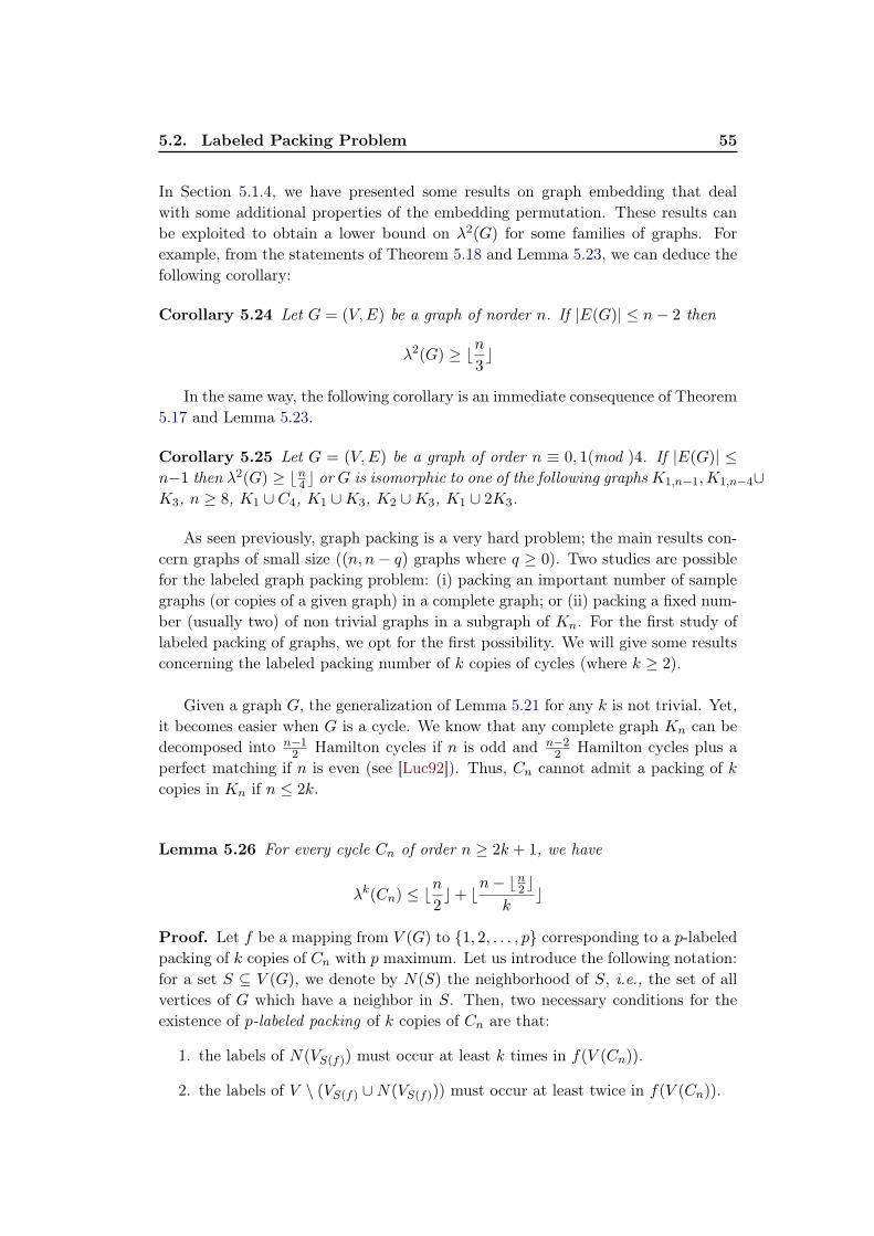
5.2. Labeled Packing Problem 55
In Section 5.1.4, we have presented some results on graph embedding that deal
with some additional properties of the embedding permutation. These results can
be exploited to obtain a lower bound on λ2(G) for some families of graphs. For
example, from the statements of Theorem 5.18 and Lemma 5.23, we can deduce the
following corollary:
Corollary 5.24 Let G = (V,E) be a graph of norder n. If |E(G)| ≤ n− 2 then
λ2(G) ≥ ⌊n
3⌋
In the same way, the following corollary is an immediate consequence of Theorem
5.17 and Lemma 5.23.
Corollary 5.25 Let G = (V,E) be a graph of order n ≡ 0, 1(mod )4. If |E(G)| ≤
n−1 then λ2(G) ≥ ⌊n4 ⌋ or G is isomorphic to one of the following graphs K1,n−1,K1,n−4∪
K3, n ≥ 8, K1 ∪ C4, K1 ∪K3, K2 ∪K3, K1 ∪ 2K3.
As seen previously, graph packing is a very hard problem; the main results con-
cern graphs of small size ((n, n− q) graphs where q ≥ 0). Two studies are possible
for the labeled graph packing problem: (i) packing an important number of sample
graphs (or copies of a given graph) in a complete graph; or (ii) packing a fixed num-
ber (usually two) of non trivial graphs in a subgraph of Kn. For the first study of
labeled packing of graphs, we opt for the first possibility. We will give some results
concerning the labeled packing number of k copies of cycles (where k ≥ 2).
Given a graph G, the generalization of Lemma 5.21 for any k is not trivial. Yet,
it becomes easier when G is a cycle. We know that any complete graph Kn can be
decomposed into n−12 Hamilton cycles if n is odd and n−2
2 Hamilton cycles plus a
perfect matching if n is even (see [Luc92]). Thus, Cn cannot admit a packing of k
copies in Kn if n ≤ 2k.
Lemma 5.26 For every cycle Cn of order n ≥ 2k + 1, we have
λk(Cn) ≤ ⌊n
2⌋+ ⌊
n− ⌊n2 ⌋
k⌋
Proof. Let f be a mapping from V (G) to {1, 2, . . . , p} corresponding to a p-labeled
packing of k copies of Cn with p maximum. Let us introduce the following notation:
for a set S ⊆ V (G), we denote by N(S) the neighborhood of S, i.e., the set of all
vertices of G which have a neighbor in S. Then, two necessary conditions for the
existence of p-labeled packing of k copies of Cn are that:
1. the labels of N(VS(f)) must occur at least k times in f(V (Cn)).
2. the labels of V \ (VS(f) ∪N(VS(f))) must occur at least twice in f(V (Cn)).
56 Chapter 5. Labeled Packing of Graphs
Hence, we have
p ≤ |VS(f)|+ ⌊|N(VS(f))|
k⌋+ ⌊
n− |VS(f)| − |N(VS(f))|
2⌋
Since k ≥ 2, the maximum value p is obtained when |VS(f)| = ⌊n2 ⌋ and |N(VS(f))| =
n− ⌊n2 ⌋, giving the desired result. �
5.2.2 Labeled-packing of k copies of cycles with order at least 4k
In this section, we determine the exact value of the labeled packing number of k
copies of cycles of order n ≥ 4k. It is done by proving that the upper bound of
Lemma 5.26 is reached for all n 6= 4k + x, where k > 2 and x mod 4 = 2.
Theorem 5.27 For every cycle Cn of order n = 2km + x, where k,m ≥ 2 andx < 2k, we have
λk(Cn) =
n2 + 1 if (x mod 4,m) = (2, 2) and k > 2.
⌊n2 ⌋+m+ 1 if x = 2k − 1.
⌊n2 ⌋+m otherwise.
Proof. Several cases are considered in this proof according to the values of x and
m. In Figure 5.6, we outline the general scheme of our proof.
Figure 5.6: Proof structure.
Case 1 : x mod 4 6= 2. Let Cn = (v1, v2, . . . , vn) be a cycle of order n, where
n ≥ 4k. From Lemma 5.26, we have λk(Cn) ≤ ⌊n2 ⌋ + ⌊
n−⌊n2⌋
k ⌋, it then suffices to
prove that Cn admits a (⌊n2 ⌋ + ⌊n−⌊n
2⌋
k ⌋)-labeled packing of k copies. In order to
simplify our proof, we consider three subcases according to the values of m and x
as follows:
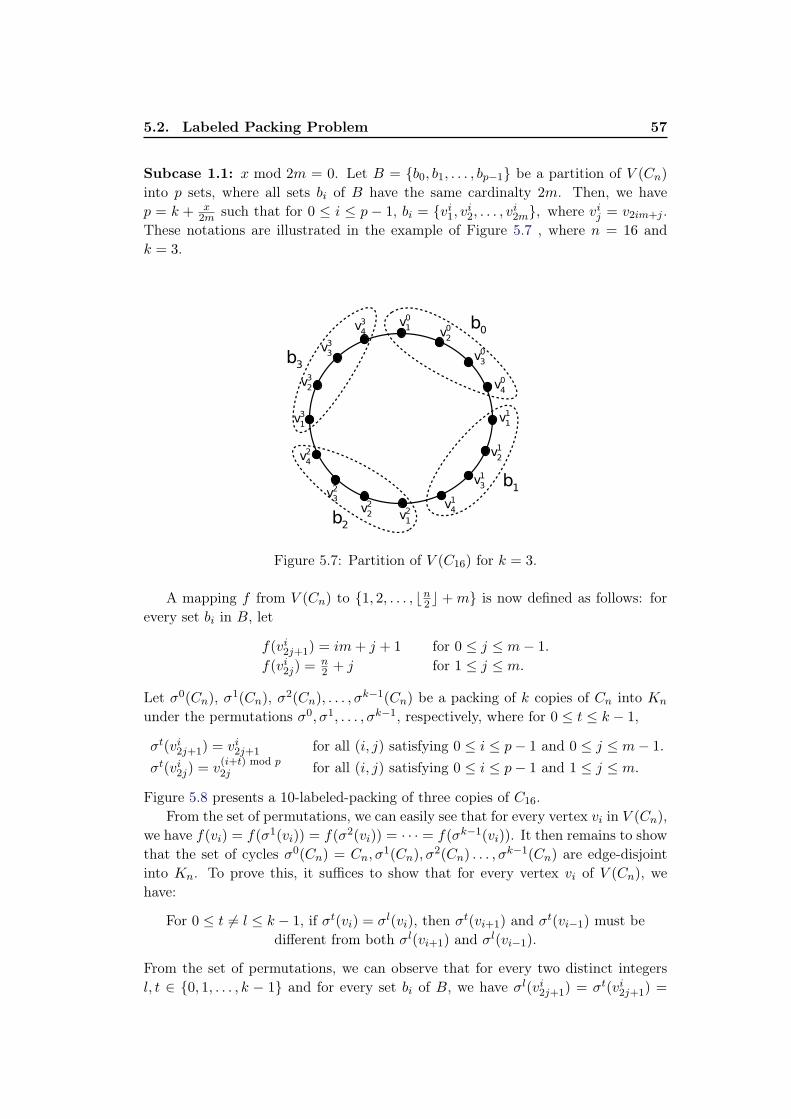
5.2. Labeled Packing Problem 57
Subcase 1.1: x mod 2m = 0. Let B = {b0, b1, . . . , bp−1} be a partition of V (Cn)
into p sets, where all sets bi of B have the same cardinalty 2m. Then, we have
p = k + x2m such that for 0 ≤ i ≤ p − 1, bi = {v
i1, v
i2, . . . , v
i2m}, where vij = v2im+j .
These notations are illustrated in the example of Figure 5.7 , where n = 16 and
k = 3.
Figure 5.7: Partition of V (C16) for k = 3.
A mapping f from V (Cn) to {1, 2, . . . , ⌊n2 ⌋ +m} is now defined as follows: for
every set bi in B, let
f(vi2j+1) = im+ j + 1 for 0 ≤ j ≤ m− 1.
f(vi2j) =n2 + j for 1 ≤ j ≤ m.
Let σ0(Cn), σ1(Cn), σ
2(Cn), . . . , σk−1(Cn) be a packing of k copies of Cn into Kn
under the permutations σ0, σ1, . . . , σk−1, respectively, where for 0 ≤ t ≤ k − 1,
σt(vi2j+1) = vi2j+1 for all (i, j) satisfying 0 ≤ i ≤ p− 1 and 0 ≤ j ≤ m− 1.
σt(vi2j) = v(i+t) mod p2j for all (i, j) satisfying 0 ≤ i ≤ p− 1 and 1 ≤ j ≤ m.
Figure 5.8 presents a 10-labeled-packing of three copies of C16.
From the set of permutations, we can easily see that for every vertex vi in V (Cn),
we have f(vi) = f(σ1(vi)) = f(σ2(vi)) = · · · = f(σk−1(vi)). It then remains to show
that the set of cycles σ0(Cn) = Cn, σ1(Cn), σ
2(Cn) . . . , σk−1(Cn) are edge-disjoint
into Kn. To prove this, it suffices to show that for every vertex vi of V (Cn), we
have:
For 0 ≤ t 6= l ≤ k − 1, if σt(vi) = σl(vi), then σt(vi+1) and σt(vi−1) must be
different from both σl(vi+1) and σl(vi−1).
From the set of permutations, we can observe that for every two distinct integers
l, t ∈ {0, 1, . . . , k − 1} and for every set bi of B, we have σl(vi2j+1) = σt(vi2j+1) =
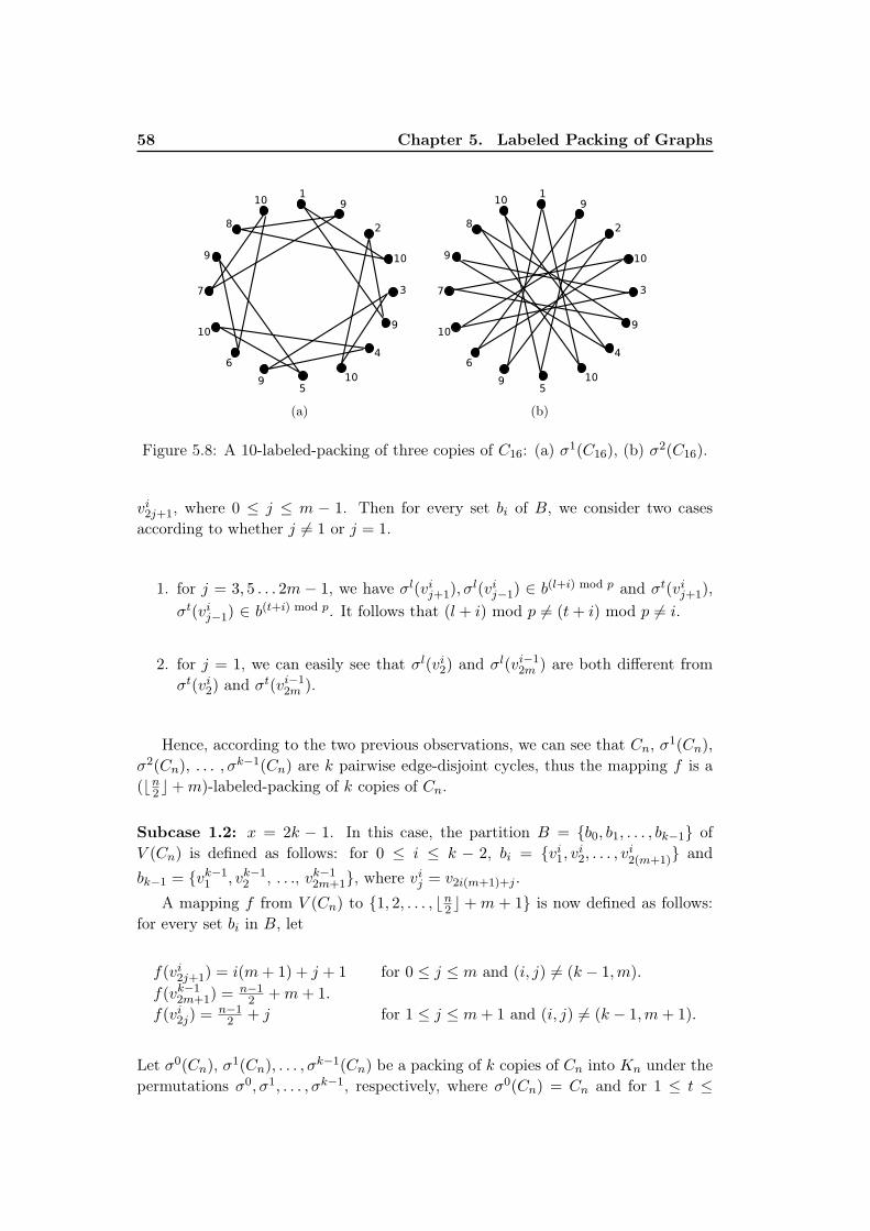
58 Chapter 5. Labeled Packing of Graphs
(a) (b)
Figure 5.8: A 10-labeled-packing of three copies of C16: (a) σ1(C16), (b) σ2(C16).
vi2j+1, where 0 ≤ j ≤ m − 1. Then for every set bi of B, we consider two cases
according to whether j 6= 1 or j = 1.
1. for j = 3, 5 . . . 2m − 1, we have σl(vij+1), σl(vij−1) ∈ b(l+i) mod p and σt(vij+1),
σt(vij−1) ∈ b(t+i) mod p. It follows that (l + i) mod p 6= (t+ i) mod p 6= i.
2. for j = 1, we can easily see that σl(vi2) and σl(vi−12m ) are both different from
σt(vi2) and σt(vi−12m ).
Hence, according to the two previous observations, we can see that Cn, σ1(Cn),
σ2(Cn), . . . , σk−1(Cn) are k pairwise edge-disjoint cycles, thus the mapping f is a
(⌊n2 ⌋+m)-labeled-packing of k copies of Cn.
Subcase 1.2: x = 2k − 1. In this case, the partition B = {b0, b1, . . . , bk−1} of
V (Cn) is defined as follows: for 0 ≤ i ≤ k − 2, bi = {vi1, vi2, . . . , v
i2(m+1)} and
bk−1 = {vk−11 , vk−1
2 , . . ., vk−12m+1}, where vij = v2i(m+1)+j .
A mapping f from V (Cn) to {1, 2, . . . , ⌊n2 ⌋ +m + 1} is now defined as follows:
for every set bi in B, let
f(vi2j+1) = i(m+ 1) + j + 1 for 0 ≤ j ≤ m and (i, j) 6= (k − 1,m).
f(vk−12m+1) =
n−12 +m+ 1.
f(vi2j) =n−12 + j for 1 ≤ j ≤ m+ 1 and (i, j) 6= (k − 1,m+ 1).
Let σ0(Cn), σ1(Cn), . . . , σ
k−1(Cn) be a packing of k copies of Cn into Kn under the
permutations σ0, σ1, . . . , σk−1, respectively, where σ0(Cn) = Cn and for 1 ≤ t ≤
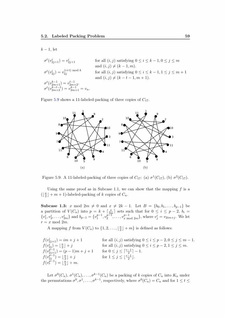
5.2. Labeled Packing Problem 59
k − 1, let
σt(vi2j+1) = vi2j+1 for all (i, j) satisfying 0 ≤ i ≤ k − 1, 0 ≤ j ≤ m
and (i, j) 6= (k − 1,m).
σt(vi2j) = v(i+t) mod k2j for all (i, j) satisfying 0 ≤ i ≤ k − 1, 1 ≤ j ≤ m+ 1
and (i, j) 6= (k − t− 1,m+ 1).
σt(vk−12m+1) = vt−1
2m+2.
σt(vk−t−12m+2 ) = vk−1
2m+1 = vn.
Figure 5.9 shows a 11-labeled-packing of three copies of C17.
(a) (b)
Figure 5.9: A 11-labeled-packing of three copies of C17: (a) σ1(C17), (b) σ2(C17).
Using the same proof as in Subcase 1.1, we can show that the mapping f is a
(⌊n2 ⌋+m+ 1)-labeled-packing of k copies of Cn.
Subcase 1.3: x mod 2m 6= 0 and x 6= 2k − 1. Let B = {b0, b1, . . . , bp−1} be
a partition of V (Cn) into p = k + ⌈ x2m⌉ sets such that for 0 ≤ i ≤ p − 2, bi =
{vi1, vi2, . . . , v
i2m} and bp−1 = {v
p−11 , vp−1
2 , . . . , vp−1x mod 2m}, where vij = v2im+j . We let
r = x mod 2m.
A mapping f from V (Cn) to {1, 2, . . . , ⌊n2 ⌋+m} is defined as follows:
f(vi2j+1) = im+ j + 1 for all (i, j) satisfying 0 ≤ i ≤ p− 2, 0 ≤ j ≤ m− 1.
f(vi2j) = ⌊n2 ⌋+ j for all (i, j) satisfying 0 ≤ i ≤ p− 2, 1 ≤ j ≤ m.
f(vp−12j+1) = (p− 1)m+ j + 1 for 0 ≤ j ≤ ⌈ r−1
2 ⌉ − 1.
f(vp−12j ) = ⌊n2 ⌋+ j for 1 ≤ j ≤ ⌊ r−1
2 ⌋.
f(vp−1r ) = ⌊n2 ⌋+m.
Let σ0(Cn), σ1(Cn), . . . , σ
k−1(Cn) be a packing of k copies of Cn into Kn under
the permutations σ0, σ1, . . . , σk−1, respectively, where σ0(Cn) = Cn and for 1 ≤ t ≤
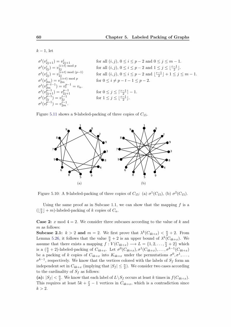
60 Chapter 5. Labeled Packing of Graphs
k − 1, let
σt(vi2j+1) = vi2j+1 for all (i, j), 0 ≤ i ≤ p− 2 and 0 ≤ j ≤ m− 1.
σt(vi2j) = v(i+t) mod p2j for all (i, j), 0 ≤ i ≤ p− 2 and 1 ≤ j ≤ ⌊ r−1
2 ⌋.
σt(vi2j) = v(i+t) mod (p−1)2j for all (i, j), 0 ≤ i ≤ p− 2 and ⌊ r−1
2 ⌋+ 1 ≤ j ≤ m− 1.
σt(vi2m) = v(i+t) mod p2m for 0 ≤ i 6= p− t− 1 ≤ p− 2.
σt(vp−t−12m ) = vp−1
r = vn.
σt(vp−12j+1) = vp−1
2j+1 for 0 ≤ j ≤ ⌈ r−12 ⌉ − 1.
σt(vp−12j ) = vt−1
2j for 1 ≤ j ≤ ⌊ r−12 ⌋.
σt(vp−1r ) = vt−1
2m .
Figure 5.11 shows a 9-labeled-packing of three copies of C15.
(a) (b)
Figure 5.10: A 9-labeled-packing of three copies of C15: (a) σ1(C15), (b) σ2(C15).
Using the same proof as in Subcase 1.1, we can show that the mapping f is a
(⌊n2 ⌋+m)-labeled-packing of k copies of Cn.
Case 2: x mod 4 = 2. We consider three subcases according to the value of k and
m as follows:
Subcase 2.1: k > 2 and m = 2. We first prove that λk(C4k+x) <n2 + 2. From
Lemma 5.26, it follows that the value n2 + 2 is an upper bound of λk(C4k+x). We
assume that there exists a mapping f : V (C4k+x) −→ L = {1, 2, . . . , n2 + 2} which
is a (n2 + 2)-labeled-packing of C4k+x. Let σ0(C4k+x), σ1(C4k+x), . . . , σ
k−1(C4k+x)
be a packing of k copies of C4k+x into K4k+x under the permutations σ0, σ1, . . . ,
σk−1, respectively. We know that the vertices colored with the labels of Sf form an
independent set in C4k+x (implying that |Sf | ≤n2 ). We consider two cases according
to the cardinality of Sf as follows:
(a): |Sf | <n2 . We know that each label of L\Sf occurs at least k times in f(C4k+x).
This requires at least 5k + x2 − 1 vertices in C4k+x, which is a contradiction since
k > 2.
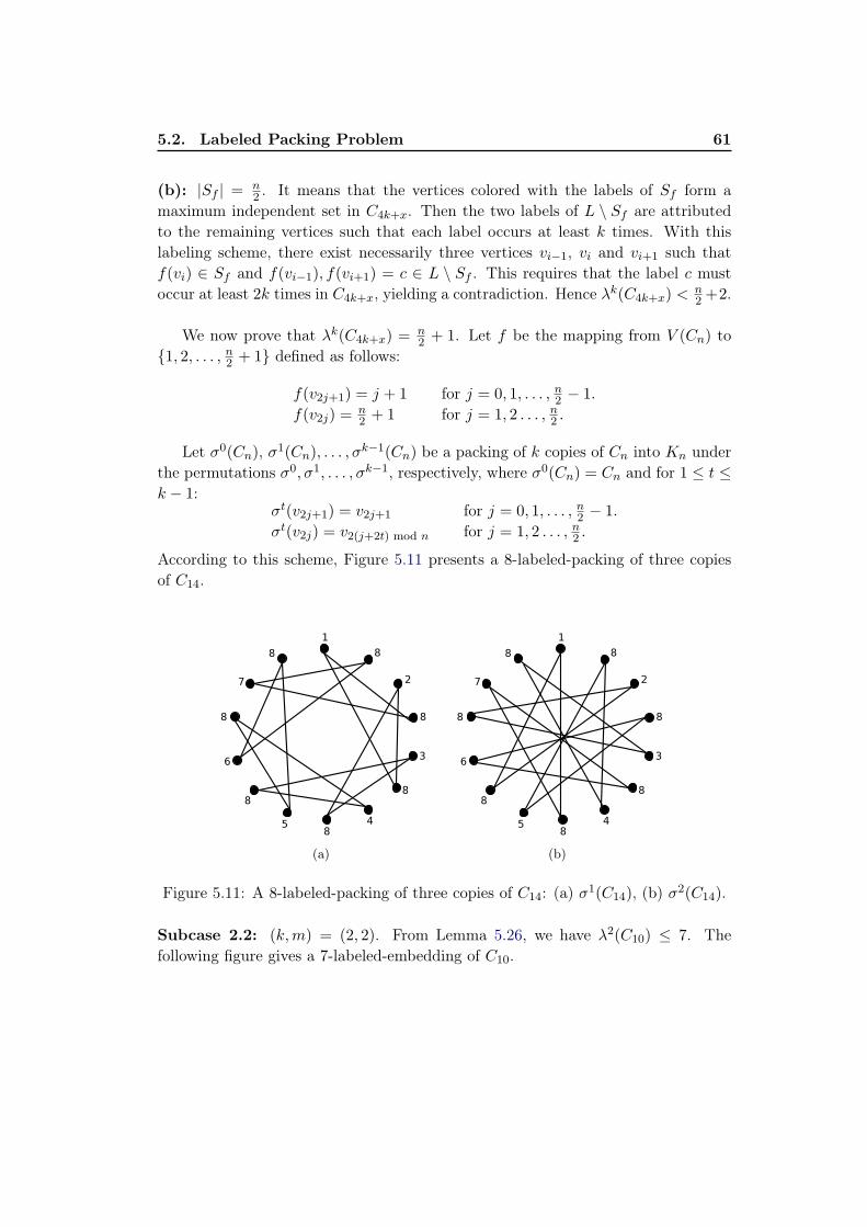
5.2. Labeled Packing Problem 61
(b): |Sf | =n2 . It means that the vertices colored with the labels of Sf form a
maximum independent set in C4k+x. Then the two labels of L \ Sf are attributed
to the remaining vertices such that each label occurs at least k times. With this
labeling scheme, there exist necessarily three vertices vi−1, vi and vi+1 such that
f(vi) ∈ Sf and f(vi−1), f(vi+1) = c ∈ L \ Sf . This requires that the label c must
occur at least 2k times in C4k+x, yielding a contradiction. Hence λk(C4k+x) <n2 +2.
We now prove that λk(C4k+x) =n2 + 1. Let f be the mapping from V (Cn) to
{1, 2, . . . , n2 + 1} defined as follows:
f(v2j+1) = j + 1 for j = 0, 1, . . . , n2 − 1.
f(v2j) =n2 + 1 for j = 1, 2 . . . , n2 .
Let σ0(Cn), σ1(Cn), . . . , σ
k−1(Cn) be a packing of k copies of Cn into Kn under
the permutations σ0, σ1, . . . , σk−1, respectively, where σ0(Cn) = Cn and for 1 ≤ t ≤
k − 1:σt(v2j+1) = v2j+1 for j = 0, 1, . . . , n2 − 1.
σt(v2j) = v2(j+2t) mod n for j = 1, 2 . . . , n2 .
According to this scheme, Figure 5.11 presents a 8-labeled-packing of three copies
of C14.
(a) (b)
Figure 5.11: A 8-labeled-packing of three copies of C14: (a) σ1(C14), (b) σ2(C14).
Subcase 2.2: (k,m) = (2, 2). From Lemma 5.26, we have λ2(C10) ≤ 7. The
following figure gives a 7-labeled-embedding of C10.
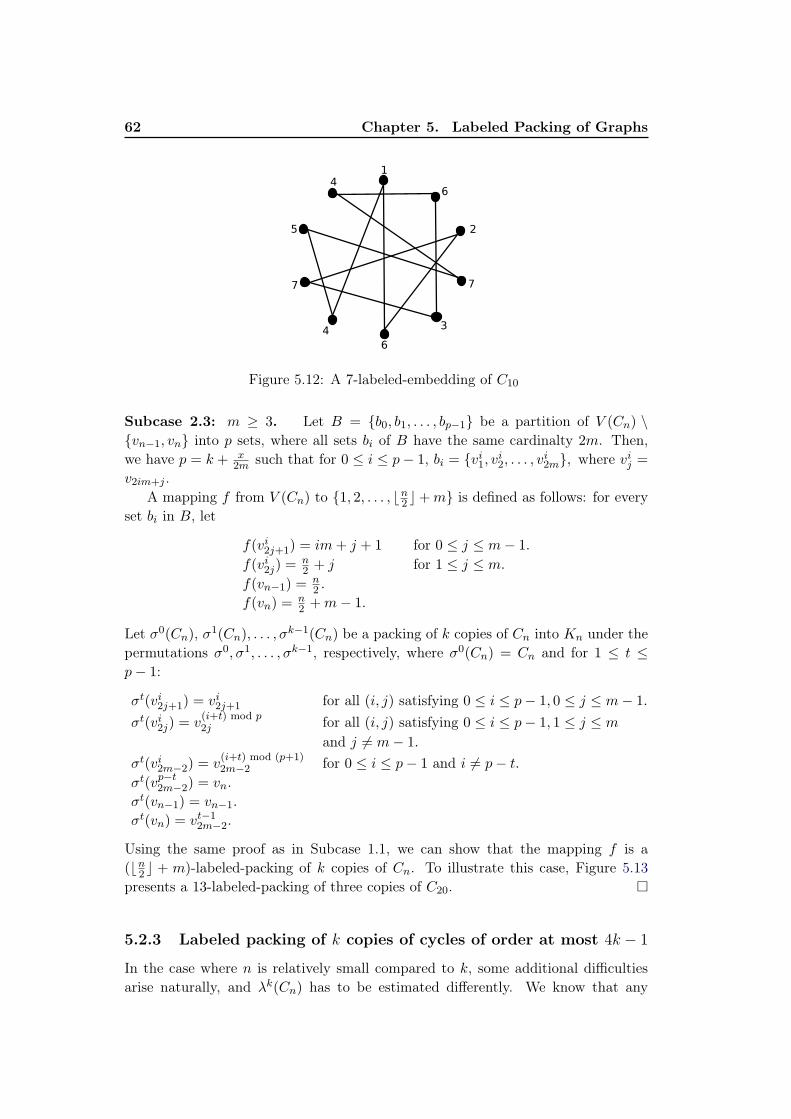
62 Chapter 5. Labeled Packing of Graphs
Figure 5.12: A 7-labeled-embedding of C10
Subcase 2.3: m ≥ 3. Let B = {b0, b1, . . . , bp−1} be a partition of V (Cn) \
{vn−1, vn} into p sets, where all sets bi of B have the same cardinalty 2m. Then,
we have p = k + x2m such that for 0 ≤ i ≤ p− 1, bi = {v
i1, v
i2, . . . , v
i2m}, where vij =
v2im+j .
A mapping f from V (Cn) to {1, 2, . . . , ⌊n2 ⌋+m} is defined as follows: for every
set bi in B, let
f(vi2j+1) = im+ j + 1 for 0 ≤ j ≤ m− 1.
f(vi2j) =n2 + j for 1 ≤ j ≤ m.
f(vn−1) =n2 .
f(vn) =n2 +m− 1.
Let σ0(Cn), σ1(Cn), . . . , σ
k−1(Cn) be a packing of k copies of Cn into Kn under the
permutations σ0, σ1, . . . , σk−1, respectively, where σ0(Cn) = Cn and for 1 ≤ t ≤
p− 1:
σt(vi2j+1) = vi2j+1 for all (i, j) satisfying 0 ≤ i ≤ p− 1, 0 ≤ j ≤ m− 1.
σt(vi2j) = v(i+t) mod p2j for all (i, j) satisfying 0 ≤ i ≤ p− 1, 1 ≤ j ≤ m
and j 6= m− 1.
σt(vi2m−2) = v(i+t) mod (p+1)2m−2 for 0 ≤ i ≤ p− 1 and i 6= p− t.
σt(vp−t2m−2) = vn.
σt(vn−1) = vn−1.
σt(vn) = vt−12m−2.
Using the same proof as in Subcase 1.1, we can show that the mapping f is a
(⌊n2 ⌋ + m)-labeled-packing of k copies of Cn. To illustrate this case, Figure 5.13
presents a 13-labeled-packing of three copies of C20. �
5.2.3 Labeled packing of k copies of cycles of order at most 4k − 1
In the case where n is relatively small compared to k, some additional difficulties
arise naturally, and λk(Cn) has to be estimated differently. We know that any

5.2. Labeled Packing Problem 63
(a) (b)
Figure 5.13: A 13-labeled-packing of three copies of C20: (a) σ1(C20), (b) σ2(C20).
complete graph Kn can be decomposed into n−12 Hamilton cycles if n is odd and
n−22 Hamilton cycles plus a perfect matching if n is even. Thus, Cn cannot admit a
packing of k copies if n ≤ 2k. After deep analysis, we raise the following conjecture.
Conjecture 5.28 For every cycle Cn of order n = 2k + x, where k ≥ 2 and 1 ≤
x ≤ 2k − 1, then
λk(Cn) =
{
2 if x = 1 and k is even.
x+ 2 otherwise .
This conjecture asserts that the upper bound of Lemma 5.26 is reached for all
n = 4k − 1, 4k − 2 and 4k − 3, where (k, n) 6= (2, 5). We report in the following the
results of our attempt to give some support to Conjecture 5.28 for some particular
cases.
Theorem 5.29 For every cycle Cn of order n = 2k+x, where k ≥ 2, 2k−3 ≤ x ≤
2k − 1 and (k, n) 6= (2, 5), we have
λk(Cn) = x+ 2
Proof. Let Cn = (v1, v2, . . . , vn) be a cycle of order n = 2k + x, where 2k − 3 ≤
x ≤ 2k − 1 and (k, n) 6= (2, 5). We know that a maximum independent set of Cn
has size ⌊n2 ⌋. Then, from Lemma 5.26, we have λk(Cn) ≤ ⌊n2 ⌋+ ⌊
n−⌊n2⌋
k ⌋ = x+2, it
then suffices to prove that Cn admits a (x+2)-labeled packing of k copies. In what
follows, we give the proof only for the case x = 2k− 1, since the proofs of the other
cases are similar.
Assume that x = 2k − 1 and let B = {b0, b1, . . . , bk−1} be a partition of
V (Cn) into k sets, such that for 0 ≤ i ≤ k − 2, bi = {vi1, vi2, v
i3, v
i4}, and bk−1 =
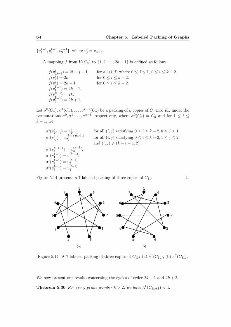
64 Chapter 5. Labeled Packing of Graphs
{vk−11 , vk−1
2 , vk−13 }, where vij = v4i+j .
A mapping f from V (Cn) to {1, 2, . . . , 2k + 1} is defined as follows:
f(vi2j+1) = 2i+ j + 1 for all (i, j) where 0 ≤ j ≤ 1, 0 ≤ i ≤ k − 2.
f(vi2) = 2k for 0 ≤ i ≤ k − 2.
f(vi4) = 2k + 1 for 0 ≤ i ≤ k − 2.
f(vk−11 ) = 2k − 1.
f(vk−12 ) = 2k.
f(vk−13 ) = 2k + 1.
Let σ0(Cn), σ1(Cn), . . . , σ
k−1(Cn) be a packing of k copies of Cn into Kn under the
permutations σ0, σ1, . . . , σk−1, respectively, where σ0(Cn) = Cn and for 1 ≤ t ≤
k − 1, let
σt(vi2j+1) = vi2j+1 for all (i, j) satisfying 0 ≤ i ≤ k − 2, 0 ≤ j ≤ 1.
σt(vi2j) = v(i+t) mod k2j for all (i, j) satisfying 0 ≤ i ≤ k − 2, 1 ≤ j ≤ 2.
and (i, j) 6= (k − t− 1, 2).
σt(vk−t−14 ) = v
(k−1)3 .
σt(vk−11 ) = v
(k−1)1 .
σt(vk−12 ) = v
(t−1)2 .
σt(vk−13 ) = v
(t−1)4 .
Figure 5.14 presents a 7-labeled packing of three copies of C11. �
(a) (b)
Figure 5.14: A 7-labeled packing of three copies of C11: (a) σ1(C11), (b) σ2(C11).
We now present our results concerning the cycles of order 2k + 1 and 2k + 2.
Theorem 5.30 For every prime number k > 2, we have λk(C2k+1) < 4.
5.2. Labeled Packing Problem 65
Proof. Let C2k+1 = (v1, v2, . . . , v2k+1, v2k+1 = v1). We assume that there exists a
mapping f : V (C2k+1) −→ L = {1, 2, 3, 4} which is a 4-labeled packing of C2k+1.
Let σ0(C2k+1), σ1(C2k+1), . . . , σ
k−1(C2k+1) be a packing of k copies of C2k+1 into
K2k+1 under the permutations σ0, σ1, . . . , σk−1, respectively. We consider two cases
according to the cardinality of Sf (which is defined in Section 5.2.1).
Case 1. |Sf | = 0. In this case, each label occurs at least twice in f(V (Cn)). Let us
introduce the following notation: for every label i of L, let Vi be the subset of vertices
with color i. We know that σ0(C2k+1) ∪ σ1(C2k+1) ∪ · · · ∪ σk−1(C2k+1) = K2k+1.
We know that all vertices of the complete graph are neighbors. Then, for every
label i of L, the number of edges in the subgraph of K2k+1 induced by the set Vi
is |Vi|(|Vi|−1)2 . Then, for every cycle σi(C2k+1) of the packing, we must have exactly
|Vi|(|Vi|−1)2k = pi edges between the vertices colored with i in the cycle σi(C2k+1).
Hence, the following system of equations must have at least one solution.
{
|Vi|(|Vi| − 1) = 2kpi for 1 ≤ i ≤ 4 (1)
|V1|+ |V2|+ |V3|+ |V4| = 2k + 1 (2)
From hypothesis, it is clear that the equation (1) has a solution if and only if
|Vi| or |Vi| − 1 are multiples of k (where 1 ≤ i ≤ 4) since k is prime. Then we have
|V1|+ |V2|+ |V3|+ |V4| > 2k + 1, therefore this system of equations has no solution
which is a contradiction for k > 2.
Case 2. |Sf | ≥ 1. Let vi be any vertex of VS(f). Then we consider two cases
according to the labels of the neighbors vertices of vi.
Subcase 1. f(vi−1) = f(vi+1) = c. In this case, we must have at least 2k vertices
colored with c. This requires at least 2k+3 vertices in C2k+1, which is a contradic-
tion.
Subcase 2. f(vi−1) 6= f(vi+1). From hypothesis, each of the two labels f(vi−1)
and f(vi+1) must occur at least k times. This requires at least 2k + 2 vertices in
C2k+1. Hence, we also reached a contradiction and the theorem is proved. �
Using the same proof as in the above theorem, we obtain the following results.
Theorem 5.31 For every even number k ≥ 2, where k is a power of 2, we haveλk(C2k+1) = 2.
Theorem 5.32 For every even number k ≥ 2, we have λk(C2k+2) < 5.
5.2.4 Summary and concluding remarks
In this section, we have proved the exact value of λk(Cn) for all k ≥ 2 and n ≥ 4k−3.
Our results are summarized in the follwoing table.
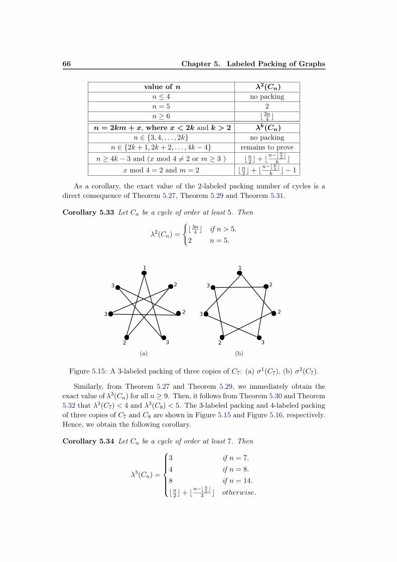
66 Chapter 5. Labeled Packing of Graphs
value of n λ2(Cn)
n ≤ 4 no packing
n = 5 2
n ≥ 6 ⌊3n4 ⌋
n = 2km + x, where x < 2k and k > 2 λk(Cn)
n ∈ {3, 4, . . . , 2k} no packing
n ∈ {2k + 1, 2k + 2, . . . , 4k − 4} remains to prove
n ≥ 4k − 3 and (x mod 4 6= 2 or m ≥ 3 ) ⌊n2 ⌋+ ⌊n−⌊n
2⌋
k ⌋
x mod 4 = 2 and m = 2 ⌊n2 ⌋+ ⌊n−⌊n
2⌋
k ⌋ − 1
As a corollary, the exact value of the 2-labeled packing number of cycles is a
direct consequence of Theorem 5.27, Theorem 5.29 and Theorem 5.31.
Corollary 5.33 Let Cn be a cycle of order at least 5. Then
λ2(Cn) =
{
⌊3n4 ⌋ if n > 5.
2 n = 5.
(a) (b)
Figure 5.15: A 3-labeled packing of three copies of C7: (a) σ1(C7), (b) σ2(C7).
Similarly, from Theorem 5.27 and Theorem 5.29, we immediately obtain the
exact value of λ3(Cn) for all n ≥ 9. Then, it follows from Theorem 5.30 and Theorem
5.32 that λ3(C7) < 4 and λ3(C8) < 5. The 3-labeled packing and 4-labeled packing
of three copies of C7 and C8 are shown in Figure 5.15 and Figure 5.16, respectively.
Hence, we obtain the following corollary.
Corollary 5.34 Let Cn be a cycle of order at least 7. Then
λ3(Cn) =
3 if n = 7.
4 if n = 8.
8 if n = 14.
⌊n2 ⌋+ ⌊n−⌊n
2⌋
3 ⌋ otherwise.
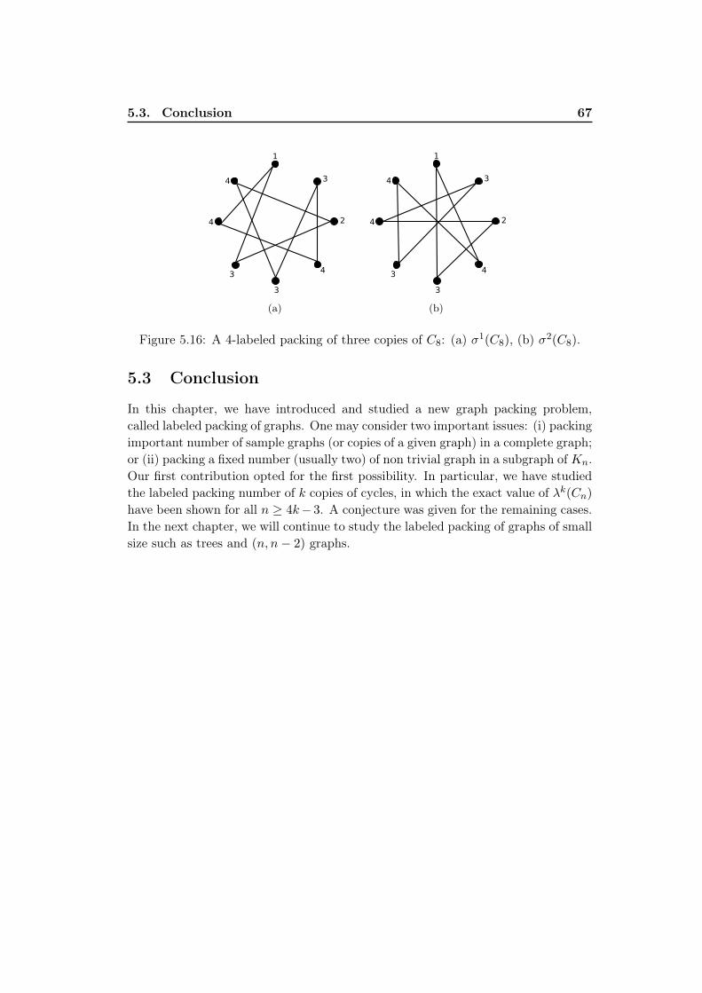
5.3. Conclusion 67
(a) (b)
Figure 5.16: A 4-labeled packing of three copies of C8: (a) σ1(C8), (b) σ2(C8).
5.3 Conclusion
In this chapter, we have introduced and studied a new graph packing problem,
called labeled packing of graphs. One may consider two important issues: (i) packing
important number of sample graphs (or copies of a given graph) in a complete graph;
or (ii) packing a fixed number (usually two) of non trivial graph in a subgraph of Kn.
Our first contribution opted for the first possibility. In particular, we have studied
the labeled packing number of k copies of cycles, in which the exact value of λk(Cn)
have been shown for all n ≥ 4k− 3. A conjecture was given for the remaining cases.
In the next chapter, we will continue to study the labeled packing of graphs of small
size such as trees and (n, n− 2) graphs.

Chapter 6
Labeled Embedding of Trees and
(n, n− 2)-graphs
Contents
6.1 Labeled fixed-point-free embedding of graphs . . . . . . . . 69
6.1.1 Labeled-embedding and labeled fixed-point-free embedding of
paths . . . . . . . . . . . . . . . . . . . . . . . . . . . . . . . 70
6.1.2 Labeled embedding of caterpillars . . . . . . . . . . . . . . . 73
6.2 Labeled embedding of trees . . . . . . . . . . . . . . . . . . . 78
6.3 Labeled embedding of (n, n− 2) graphs . . . . . . . . . . . . . 84
6.4 Conclusion . . . . . . . . . . . . . . . . . . . . . . . . . . . . . 87
This chapter deals with the labeled embedding of trees and (n, n−2)-graphs. In
Section 6.1, we will introduce a new labeled embedding problem called labeled fixed-point-free embedding of graphs (i.e., a labeled embedding without fixed vertices).
Then we will show that the correlation between this problem and the labeled em-
bedding problem allows to derive some results on λ2(G). In Section 6.2, we present
some results on the labeled embedding number of a tree. Finally, in Section 6.3, an
upper bound on the labeled embedding number of (n, n− 2)-graphs is proposed.
6.1 Labeled fixed-point-free embedding of graphs
In correlation with the labeled embedding number, we introduce a new embedding
problem called labeled fixed-point-free embedding of graphs.
Definition 6.1 Let f be a mapping from V (G) to L = {1, 2, . . . , p}, which is alabeled embedding of G with p labels under the permutation σ. We say that f is alabeled fixed-point-free embedding if σ is a fixed-point-free permutation.
The maximum positive integer p for which G admits a labeled fixed-point-free
embedding of G is called the labeled fixed-point-free embedding number and is de-
noted by α2(G).
The following lemma shows an upper bound on α2(G).
70 Chapter 6. Labeled Embedding of Trees and (n, n− 2)-graphs
Lemma 6.1 Let G be a graph of order n. If there exists an embedding of G intoKn, then
α2(G) ≤ ⌊n
2⌋.
Proof. We can easily verify that a necessary condition for the existence of p-labeledfixed-point-free embedding of G is that every label of L occurs at least twice in G,
i.e., the upper bound of α2(G) is reached if and only if we find an embedding of G
having all its cycles of length two (except one of length three if n is odd). Hence,
α2(G) ≤ ⌊n2 ⌋. �
Given a graph G, the following lemma shows a lower bound on λ2(G) in terms of
α2(G) as follows:
Lemma 6.2 Let G be a graph of order n and let X be any set of end vertices of G.If there exists a fixed-point-free embedding of G[V \X] with p labels into Kn, then
λ2(G) ≥ |X|+ p
Proof. By hypothesis, there exists a permutation σ′ on V (T ) such that σ′ is a
fixed-point-free embedding with p labels. This permutation can be extended to a
permutation σ on G as follows:
σ(x) = x for all x ∈ X and σ(y) = σ′(y) for all y ∈ V \X
From this permutation function, it is clear that for every edge xy ∈ E(G) such that
x ∈ X and y ∈ V \X, we have σ(x)σ(y) /∈ E(G). Hence λ2(G) ≥ |X|+ p. �
We can conclude that the correlation between the two parameters λ2(G) and α2(G)
allows to reach the upper bound of Lemma 5.21 if there is a maximum independent
set in G with only vertices of degree 1.
As we have seen in Lemma 5.23, we can obtain the following lower bound on
α2(G) which is related to the permutation structure.
Lemma 6.3 Let G be a graph. If G has a fixed-point-free embedding σ with p cycles,then
α2(G) ≥ p.
We note that the parameter α2(G) will be used frequently to prove the main results
of the next section.
6.1.1 Labeled-embedding and labeled fixed-point-free embedding
of paths
We first determine the exact value of the labeled embedding number of paths. It
is done by proving that the upper bound of Lemma 5.21 is reached for all paths of
order at least 5.
6.1. Labeled fixed-point-free embedding of graphs 71
Theorem 6.4 Let Pn be a path of order at least 4. Then
λ2(Pn) =
⌊3n4 ⌋ if n mod 4 = 0, 2, 3 and n > 4,
⌊3n4 ⌋+ 1 if n mod 4 = 1 and n > 5,
3 if n = 5,
1 if n = 4.
Proof. Let Pn = (v1, v2, . . . , vn) be a path of order n where n ≥ 4. We consider
four cases as follows:
Case 1: n mod 4 = 0, 2, 3 and n > 4. From Lemma 5.21, we have λ2(Pn) ≤ ⌊3n4 ⌋,
it then suffices to prove that Pn admits a ⌊3n4 ⌋-labeled embedding. Since Pn is a
spanning subgraph of Cn, By putting together Lemma 5.20 and Corollary 5.33, we
get λ2(Pn) ≥ λ2(Cn) = ⌊3n4 ⌋.
Case 2: n = 4m+ 1 and m ≥ 2. A mapping f : V (Pn) −→ {1, 2, . . . , ⌊3n4 ⌋+ 1} is
defined as follows:
f(v2i+1) = i+ 1 for i = 0 . . . 2m.
f(v2i) = 2m+ i+ 1 for i = 1 . . .m.
f(v2i) = m+ i+ 1 for i = m+ 1 . . . 2m.
Let σ(Pn) be the embedding of Pn in Kn under the permutation σ where
σ(v2i+1) = v2i+1 for i = 0 . . . 2m.
σ(v2i) = v2(m+i) for i = 1 . . .m.
σ(v2i) = v2(i−m) for i = m+ 1 . . . 2m.
This permutation induces the following path:
σ(Pn) = v1, v2m+2, v3, v2m+4 . . . v2m+1, v2, v2m+3, v4, v2m+5 . . . v2m, v4m+1
According to the permutation σ, it is clear that for every vertex vi in V (Pn), we
have f(vi) = f(σ(vi)). It now remains to show that Pn and σ(Pn) are edge-disjoint.
To do so, it suffices to show that:
for every vertex vi of Pn, if σ(vi) = vi then σ(vi+1) /∈ {vi−1, vi+1}.
From the permutation σ, we have σ(vi) = vi if and only if i is odd. Then we
consider four cases for the vertices σ(vi+1) and σ(vi−1):
1. for i = 1, we have σ(v2) = v2m+2.
2. for i = 3, 5, . . . 2m−1, we have vi−1, vi+1 ∈ {v2, v4, . . . , v2m} and σ(vi−1), σ(vi+1) ∈
{v2m+2, v2m+4, . . . , v4m}.
3. for i = 2m+ 1, we have σ(v2m) = v4m and σ(v2m+2) = v2.

72 Chapter 6. Labeled Embedding of Trees and (n, n− 2)-graphs
4. for i = 2m+3, . . . 4m−3, we have vi−1, vi+1 ∈ {v2m+2, v2m+4, . . . , v4m−2} and
σ(vi−1), σ(vi+1) ∈ {v2, v4, . . . , v2m−2}.
5. for i = 4m− 1, we have σ(v4m) = v2m.
According to the previous observations, we get that E(Pn) ∩ E(σ(Pn)) = ∅ for
m ≥ 2, thus the mapping f is a (⌊3n4 ⌋+ 1)-labeled-embedding of Pn.
Case 3: n = 5. We first prove that λ2(P5) < 4. We assume that there ex-
ists a mapping f : V (P5) −→ L = {1, 2, 3, 4} which is 4-labeled embedding of
P5. We can easily see that the existence of this 4-labeled embedding requires the
existence of three independent vertices v1, v3 and v5 colored with three different
labels {c1, c2, c3} ⊂ L, then the two vertices v2 and v4 are colored with the same
label of L \ {c1, c2, c3}. We can easily see that this coloring scheme is not 4-labeled
embedding of P5 which is a contradiction with the hypothesis. We conclude that
λ2(Pn) < 4. It then remains to show that λ2(P5) = 3. This is proved by Figure 6.1.
Figure 6.1: A 3-labeled embedding of P5.
Case 4: n = 4. We can easily see that there is an unique embedding of P4 into
K4 (Figure 6.2). This embedding scheme gives λ2(P4) = 1. �
Figure 6.2: A 1-labeled embedding of P4.
We now study the labeled fixed-point-free embedding number of paths. This
result is crucial for the proof of our result in the next section.
Theorem 6.5 Let Pn be a path of order at least 4, then
α2(Pn) =
{
⌊n2 ⌋ if n > 5,
1 if n = 4, 5.
Proof. Let Pn = (v1, v2, . . . , vn) be a path of order n where n ≥ 4. We consider
two cases depending on whether n > 5 or n ≤ 5.
Case 1: n > 5. From Lemma 6.1, we know that α(Pn) ≤ ⌊n2 ⌋. It now suffices to
prove that Pn admits a ⌊n2 ⌋-labeled fixed-point-free embedding into Kn. We consider
two subcases as follows:
Subcase 1: n is even. We divide P into three subpaths as follows:
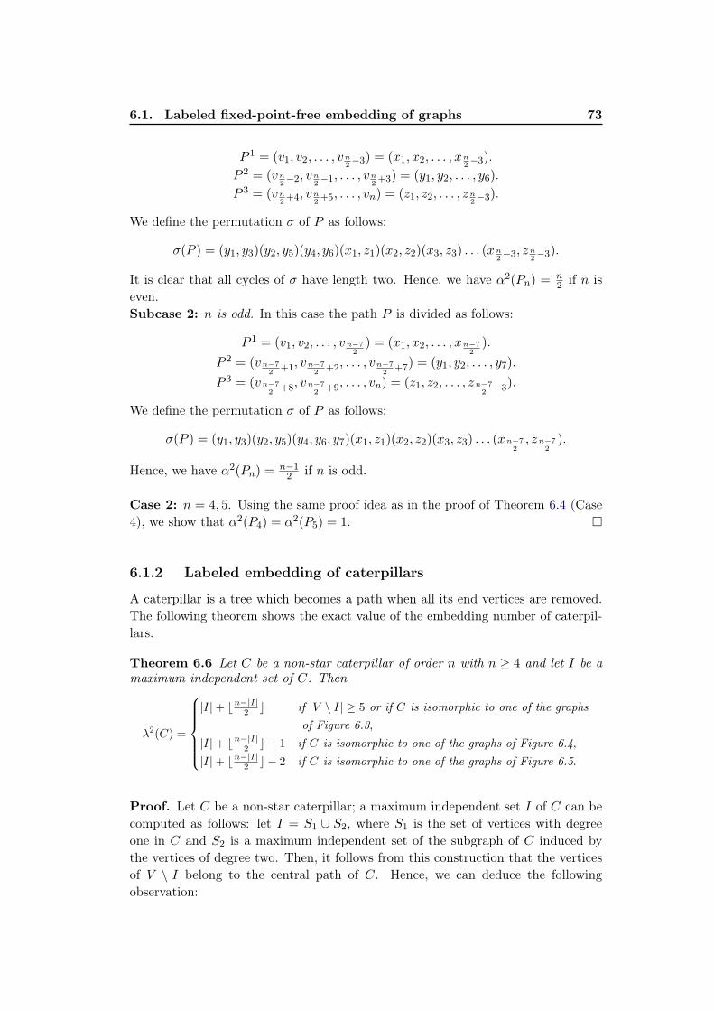
6.1. Labeled fixed-point-free embedding of graphs 73
P 1 = (v1, v2, . . . , vn2−3) = (x1, x2, . . . , xn
2−3).
P 2 = (vn2−2, vn
2−1, . . . , vn
2+3) = (y1, y2, . . . , y6).
P 3 = (vn2+4, vn
2+5, . . . , vn) = (z1, z2, . . . , zn
2−3).
We define the permutation σ of P as follows:
σ(P ) = (y1, y3)(y2, y5)(y4, y6)(x1, z1)(x2, z2)(x3, z3) . . . (xn2−3, zn
2−3).
It is clear that all cycles of σ have length two. Hence, we have α2(Pn) =n2 if n is
even.
Subcase 2: n is odd. In this case the path P is divided as follows:
P 1 = (v1, v2, . . . , vn−72) = (x1, x2, . . . , xn−7
2).
P 2 = (vn−72
+1, vn−72
+2, . . . , vn−72
+7) = (y1, y2, . . . , y7).
P 3 = (vn−72
+8, vn−72
+9, . . . , vn) = (z1, z2, . . . , zn−72
−3).
We define the permutation σ of P as follows:
σ(P ) = (y1, y3)(y2, y5)(y4, y6, y7)(x1, z1)(x2, z2)(x3, z3) . . . (xn−72, zn−7
2).
Hence, we have α2(Pn) =n−12 if n is odd.
Case 2: n = 4, 5. Using the same proof idea as in the proof of Theorem 6.4 (Case
4), we show that α2(P4) = α2(P5) = 1. �
6.1.2 Labeled embedding of caterpillars
A caterpillar is a tree which becomes a path when all its end vertices are removed.
The following theorem shows the exact value of the embedding number of caterpil-
lars.
Theorem 6.6 Let C be a non-star caterpillar of order n with n ≥ 4 and let I be amaximum independent set of C. Then
λ2(C) =
|I|+ ⌊n−|I|2⌋ if |V \ I| ≥ 5 or if C is isomorphic to one of the graphs
of Figure 6.3,
|I|+ ⌊n−|I|2⌋ − 1 if C is isomorphic to one of the graphs of Figure 6.4,
|I|+ ⌊n−|I|2⌋ − 2 if C is isomorphic to one of the graphs of Figure 6.5.
Proof. Let C be a non-star caterpillar; a maximum independent set I of C can be
computed as follows: let I = S1 ∪ S2, where S1 is the set of vertices with degree
one in C and S2 is a maximum independent set of the subgraph of C induced by
the vertices of degree two. Then, it follows from this construction that the vertices
of V \ I belong to the central path of C. Hence, we can deduce the following
observation:

74 Chapter 6. Labeled Embedding of Trees and (n, n− 2)-graphs
(a)
(b)
(c)
(d)
>0 >=0
v2v
3 v4 v5
>0v1
(e)
(f) (g)
>0
v1v
2 v3 v4
>0>0v5
(h)
Figure 6.3: Caterpillars with λ2(G) = |I|+ ⌊n−|I|2 ⌋
Observation 6.7 The induced subgraph G[V \ I] is a set of paths.
Let f be a vertex labeling of C and let σ(C) be an embedding of C into Kn
under the permutation σ. We distinguish three cases according to the cardinality
of V \ I as follows:
Case 1: |V \ I| ≥ 5 or C is isomorphic to one of the graphs of Figure. 6.3. From
Lemma 5.21, we have λ2(C) ≤ |I|+ ⌊n−|I|2 ⌋, it then suffices to prove that C admits
a (|I|+ ⌊n−|I|2 ⌋)-labeled embedding. Three subcases are considered as follows:
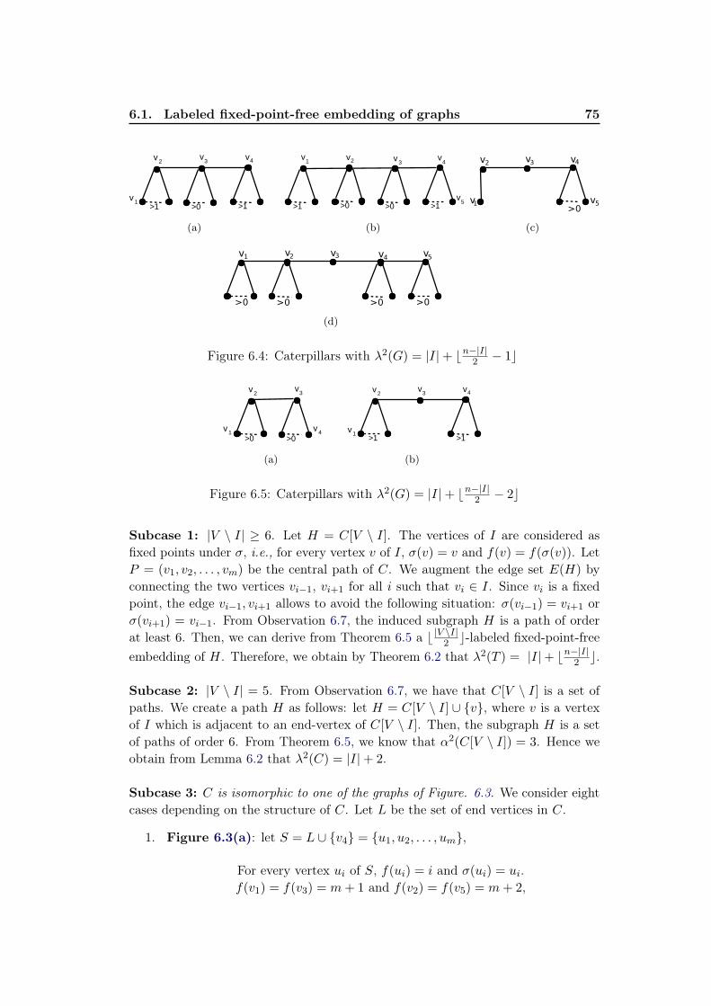
6.1. Labeled fixed-point-free embedding of graphs 75
>1 >0
v2v
3 v4
>1v1
(a)
>1
v1 v2 v3
>0
v4
>1>0v
5
(b) (c)
(d)
Figure 6.4: Caterpillars with λ2(G) = |I|+ ⌊n−|I|2 − 1⌋
>0 >0
v2v
3
v1 v4
(a)
>1 >1
v2v
3 v4
v1
(b)
Figure 6.5: Caterpillars with λ2(G) = |I|+ ⌊n−|I|2 − 2⌋
Subcase 1: |V \ I| ≥ 6. Let H = C[V \ I]. The vertices of I are considered as
fixed points under σ, i.e., for every vertex v of I, σ(v) = v and f(v) = f(σ(v)). Let
P = (v1, v2, . . . , vm) be the central path of C. We augment the edge set E(H) by
connecting the two vertices vi−1, vi+1 for all i such that vi ∈ I. Since vi is a fixed
point, the edge vi−1, vi+1 allows to avoid the following situation: σ(vi−1) = vi+1 or
σ(vi+1) = vi−1. From Observation 6.7, the induced subgraph H is a path of order
at least 6. Then, we can derive from Theorem 6.5 a ⌊ |V \I|2 ⌋-labeled fixed-point-free
embedding of H. Therefore, we obtain by Theorem 6.2 that λ2(T ) = |I|+ ⌊n−|I|2 ⌋.
Subcase 2: |V \ I| = 5. From Observation 6.7, we have that C[V \ I] is a set of
paths. We create a path H as follows: let H = C[V \ I] ∪ {v}, where v is a vertex
of I which is adjacent to an end-vertex of C[V \ I]. Then, the subgraph H is a set
of paths of order 6. From Theorem 6.5, we know that α2(C[V \ I]) = 3. Hence we
obtain from Lemma 6.2 that λ2(C) = |I|+ 2.
Subcase 3: C is isomorphic to one of the graphs of Figure. 6.3. We consider eight
cases depending on the structure of C. Let L be the set of end vertices in C.
1. Figure 6.3(a): let S = L ∪ {v4} = {u1, u2, . . . , um},
For every vertex ui of S, f(ui) = i and σ(ui) = ui.
f(v1) = f(v3) = m+ 1 and f(v2) = f(v5) = m+ 2,
76 Chapter 6. Labeled Embedding of Trees and (n, n− 2)-graphs
σ(v1) = v3, σ(v3) = v1, σ(v2) = v5 and σ(v5) = v2.
2. Figure 6.3(b): let S = L ∪ {v3, v5} = {u1, u2, . . . , um},
For every vertex ui of S, f(ui) = i and σ(ui) = ui.
f(v1) = f(v4) = m+ 1 and f(v2) = f(v6) = m+ 2.
σ(v1) = v4, σ(v4) = v1, σ(v2) = v6 and σ(v6) = v2.
3. Figure 6.3(c): let S = L ∪ {v2, v4, v6} = {u1, u2, . . . , um},
For every vertex ui of S, f(ui) = i and σ(ui) = ui.
f(v1) = f(v5) = m+ 1 and f(v3) = f(v7) = m+ 2.
σ(v1) = v5, σ(v5) = v1, σ(v3) = v7 and σ(v7) = v3.
4. Figure 6.3(d): let S = L ∪ {v2, v5} = {u1, u2, . . . , um},
For every vertex ui of S, f(ui) = i and σ(ui) = ui.
f(v1) = f(v4) = m+ 1, f(v3) = f(v6) = m+ 2 .
σ(v1) = v4, σ(v4) = v1, σ(v3) = v6 and σ(v6) = v3.
5. Figure 6.3(e): let S = (L \ {v1}) ∪ {v4} = {u1, u2, . . . , um},
For every vertex ui of S, f(ui) = i and σ(ui) = ui.
f(v1) = f(v3) = m+ 1 and f(v2) = f(v5) = m+ 2.
σ(v1) = v3, σ(v3) = v1, σ(v2) = v5 and σ(v5) = v2.
6. Figure 6.3(f): let S = L ∪ {v4} = {u1, u2, . . . , um},
For every vertex ui of S, f(ui) = i and σ(ui) = ui.
f(v1) = f(v3) = m+ 1 and f(v2) = f(v5) = m+ 2.
σ(v1) = v3, σ(v3) = v1, σ(v2) = v5, and σ(v5) = v2.
7. Figure 6.3(g): let S = (L \ {v1, v5}) ∪ {v4} = {u1, u2, . . . , um},
For every vertex ui of S, f(ui) = i and σ(ui) = ui.
f(v1) = f(v3) = m+ 1 and f(v2) = f(v5) = m+ 2.
σ(v1) = v3, σ(v3) = v1 ,σ(v2) = v5, and σ(v5) = v2.
8. Figure 6.3(h): let S = (L \ {v5}) ∪ {v4} = {u1, u2, . . . , um},

6.1. Labeled fixed-point-free embedding of graphs 77
For every vertex ui of S, f(ui) = i and σ(ui) = ui.
f(v1) = f(v3) = m+ 1 and f(v2) = f(v5) = m+ 2.
σ(v1) = v3, σ(v2) = v5, σ(v3) = v1 and σ(v5) = v2.
Case 2: C is isomorphic to one of the graphs of Figure 6.4. We can easily check
that λ2(C) ≤ |I|+⌊n−|I|2 ⌋−1. It then suffices to prove that λ2(C) ≥ |I|+⌊n−|I|
2 ⌋−1
for every graph of Figure 6.4.
1. Figure 6.4(a): let S = L \ {v1} = {u1, u2, . . . , um},
For every vertex ui of S, f(ui) = i and σ(ui) = ui.
f(v1) = f(v2) = f(v3) = f(v4) = m+ 1.
σ(v1) = v3, σ(v2) = v1, σ(v3) = v4 and σ(v4) = v2.
2. Figure 6.4(b): let S = L{u1, u2, . . . , um},
For every vertex ui of S, f(ui) = i and σ(ui) = ui.
f(v1) = f(v2) = f(v3) = f(v4) = m+ 1.
σ(v1) = v3, σ(v2) = v1, σ(v3) = v4 and σ(v4) = v2.
3. Figure 6.4(c): let S = (L ∪ {v1, v5}) ∪ {v2} = {u1, u2, . . . , um},
For every vertex ui of S, f(ui) = i and σ(ui) = ui.
f(v1) = f(v4) = m+ 1, f(v3) = f(v5) = m+ 2.
σ(v1) = v4, σ(v4) = v1, σ(v3) = v5 and σ(v5) = v3.
4. Figure 6.4(d): let S = (L \ ∪{v3} = {u1, u2, . . . , um},
For every vertex ui of S, f(ui) = i and σ(ui) = ui.
f(v1) = f(v2) = f(v3) = f(v4) = m+ 1.
σ(v1) = v3, σ(v2) = v1, σ(v3) = v4 and σ(v4) = v2.
Case 3: C is isomorphic to one of the graphs of Figure 6.5. In this case, we can
also check that λ2(C) ≤ |I| + ⌊n−|I|2 ⌋ − 2. It then suffices to prove that λ2(T ) ≥
|I|+ ⌊n−|I|2 ⌋ − 2 for every graph of Figure 6.5.
1. Figure 6.5(a): let S = L \ {v1, v4} = {u1, u2, . . . , um},
For every vertex ui of S, f(ui) = i and σ(ui) = ui.
f(v1) = f(v2) = f(v3) = f(v4) = m+ 1.
σ(v1) = v2, σ(v2) = v4, σ(v3) = v1 and σ(v4) = v3.
78 Chapter 6. Labeled Embedding of Trees and (n, n− 2)-graphs
2. Figure 6.5(b): let S = L \ {v1} = {u1, u2, . . . , um},
For every vertex ui of S, f(ui) = i and σ(ui) = ui.
f(v1) = f(v2) = f(v3) = f(v4) = m+ 1.
σ(v1) = v2, σ(v2) = v4, σ(v3) = v1 and σ(v4) = v3.
�
6.2 Labeled embedding of trees
In this section, we intend to prove a lower bound on the labeled embedding number
of general trees.
Theorem 6.8 Let T be a non-star tree of order n and let X be the set of end-verticesof T , then
λ2(T ) ≥ max(|X|+ ⌊n−|X|2 ⌋ − 1, ⌊3n4 ⌋ − 2) if T \X 6= K1,n−1,
λ2(T ) ≥ ⌊3n4 ⌋ − 2 otherwise.
The lower bound of the previous theorem relies on two main theorems (Theorem
6.10 and Theorem 6.11). We first introduce the following notation to simplify our
proofs. Let T = (V,E) be a graph of order n. For a vertex v ∈ V , let d(v) denote
its degree and let diam(T ) denote the diameter of T . A permutation σ of V (T ) will
be called good for T if and only if:
1. σ is an embedding of T .
2. σ has at least ⌊3n4 ⌋ − 2 cycles.
3. for every pair of end-vertices (u, v) in T , we have σ(u) 6= v and σ(v) 6= u.
Thus, to prove that λ2(T ) ≥ ⌊3n4 ⌋ − 2, it suffices to show that T admits a good
permutation. Finally, for a vertex v of T , let Tv be the subtree rooted at v and let
V (Tv) denote the set of vertices of Tv. At the beginning, we prove the following
theorem which will be useful for the proof of Theorem 6.10.
Theorem 6.9 Let T be a tree of order n and diameter 4, then there exists anembedding σ of T such that σ is good.
Proof. If T is a caterpillar, then we have by Theorem 6.6 that λ2(T ) ≥ ⌊3n4 ⌋ − 2.
In the other case, the level 2 of T contains at least three vertices of degree greater
than 1 (see Figure 6.6). Let U = {u1, u2, . . . , um} be the set of vertices of T with
degree at least 2 except x and y. Let σ(T ) be an embedding of T into Kn under the
permutation σ where
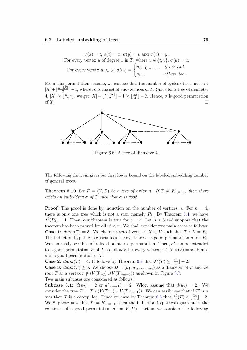
6.2. Labeled embedding of trees 79
σ(x) = t, σ(t) = x, σ(y) = v and σ(v) = y.
For every vertex u of degree 1 in T , where u /∈ {t, v}, σ(u) = u.
For every vertex ui ∈ U , σ(ui) =
{
u(i+1) mod m if i is odd ,
ui−1 otherwise.
From this permutation scheme, we can see that the number of cycles of σ is at least
|X|+⌊n−|X|2 ⌋−1, where X is the set of end-vertices of T . Since for a tree of diameter
4, |X| ≥ ⌊n−12 ⌋, we get |X|+ ⌊n−|X|
2 ⌋− 1 ≥ ⌊3n4 ⌋− 2. Hence, σ is good permutation
of T . �
Figure 6.6: A tree of diameter 4.
The following theorem gives our first lower bound on the labeled embedding number
of general trees.
Theorem 6.10 Let T = (V,E) be a tree of order n. If T 6= K1,n−1, then thereexists an embedding σ of T such that σ is good.
Proof. The proof is done by induction on the number of vertices n. For n = 4,
there is only one tree which is not a star, namely P4. By Theorem 6.4, we have
λ2(P4) = 1. Then, our theorem is true for n = 4. Let n ≥ 5 and suppose that the
theorem has been proved for all n′ < n. We shall consider two main cases as follows:
Case 1: diam(T ) = 3. We choose a set of vertices X ⊂ V such that T \X = P4.
The induction hypothesis guarantees the existence of a good permutation σ′ on P4.
We can easily see that σ′ is fixed-point-free permutation. Then, σ′ can be extended
to a good permutation σ of T as follows: for every vertex x ∈ X,σ(x) = x. Hence
σ is a good permutation of T .
Case 2: diam(T ) = 4. It follows by Theorem 6.9 that λ2(T ) ≥ ⌊3n4 ⌋ − 2.
Case 3: diam(T ) ≥ 5. We choose D = (u1, u1, . . . , um) as a diameter of T and we
root T at a vertex r /∈ (V (Tu2) ∪ V (Tum−1)) as shown in Figure 6.7.
Two main subcases are considered as follows:
Subcase 3.1: d(u2) = 2 or d(um−1) = 2. Wlog, assume that d(u2) = 2. We
consider the tree T ′ = T \ (V (Tu2) ∪ V (Tum−1)). We can easily see that if T ′ is a
star then T is a caterpillar. Hence we have by Theorem 6.6 that λ2(T ) ≥ ⌊3n4 ⌋ − 2.
We Suppose now that T ′ 6= K1,m−1, then the induction hypothesis guarantees the
existence of a good permutation σ′ on V (T ′). Let us we consider the following
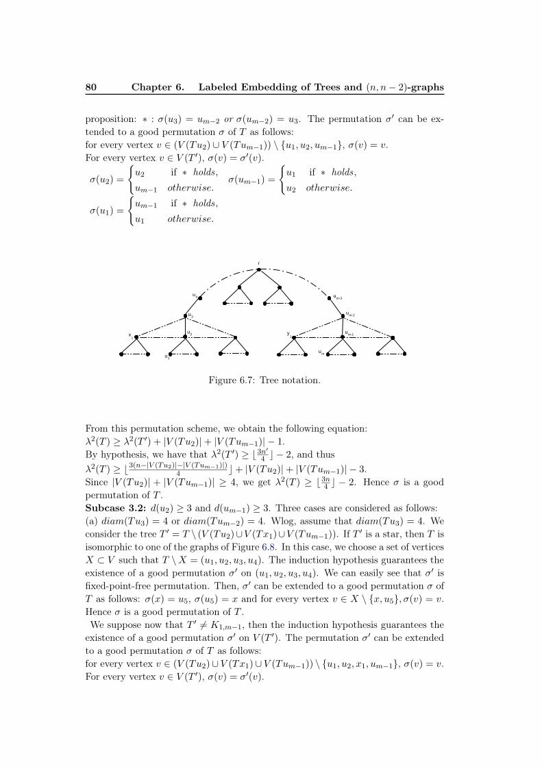
80 Chapter 6. Labeled Embedding of Trees and (n, n− 2)-graphs
proposition: ∗ : σ(u3) = um−2 or σ(um−2) = u3. The permutation σ′ can be ex-
tended to a good permutation σ of T as follows:
for every vertex v ∈ (V (Tu2) ∪ V (Tum−1)) \ {u1, u2, um−1}, σ(v) = v.
For every vertex v ∈ V (T ′), σ(v) = σ′(v).
σ(u2) =
{
u2 if ∗ holds,
um−1 otherwise.σ(um−1) =
{
u1 if ∗ holds,
u2 otherwise.
σ(u1) =
{
um−1 if ∗ holds,
u1 otherwise.
um-2
um-1
um
u3
u2
u1
x1
u4 um-3
r
y1
Figure 6.7: Tree notation.
From this permutation scheme, we obtain the following equation:
λ2(T ) ≥ λ2(T ′) + |V (Tu2)|+ |V (Tum−1)| − 1.
By hypothesis, we have that λ2(T ′) ≥ ⌊3n′
4 ⌋ − 2, and thus
λ2(T ) ≥ ⌊3(n−|V (Tu2)|−|V (Tum−1)|)4 ⌋+ |V (Tu2)|+ |V (Tum−1)| − 3.
Since |V (Tu2)| + |V (Tum−1)| ≥ 4, we get λ2(T ) ≥ ⌊3n4 ⌋ − 2. Hence σ is a good
permutation of T .
Subcase 3.2: d(u2) ≥ 3 and d(um−1) ≥ 3. Three cases are considered as follows:
(a) diam(Tu3) = 4 or diam(Tum−2) = 4. Wlog, assume that diam(Tu3) = 4. We
consider the tree T ′ = T \ (V (Tu2)∪V (Tx1)∪V (Tum−1)). If T ′ is a star, then T is
isomorphic to one of the graphs of Figure 6.8. In this case, we choose a set of vertices
X ⊂ V such that T \X = (u1, u2, u3, u4). The induction hypothesis guarantees the
existence of a good permutation σ′ on (u1, u2, u3, u4). We can easily see that σ′ is
fixed-point-free permutation. Then, σ′ can be extended to a good permutation σ of
T as follows: σ(x) = u5, σ(u5) = x and for every vertex v ∈ X \ {x, u5}, σ(v) = v.
Hence σ is a good permutation of T .
We suppose now that T ′ 6= K1,m−1, then the induction hypothesis guarantees the
existence of a good permutation σ′ on V (T ′). The permutation σ′ can be extended
to a good permutation σ of T as follows:
for every vertex v ∈ (V (Tu2)∪ V (Tx1)∪ V (Tum−1)) \ {u1, u2, x1, um−1}, σ(v) = v.
For every vertex v ∈ V (T ′), σ(v) = σ′(v).
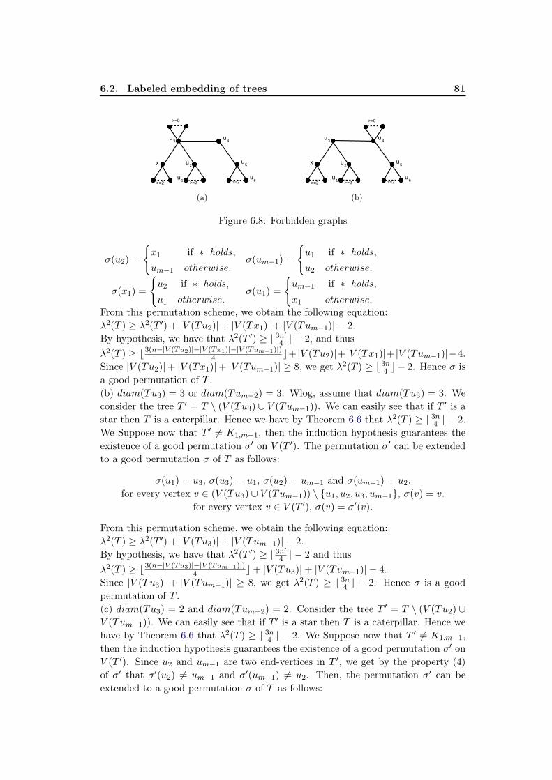
6.2. Labeled embedding of trees 81
>=2>=2 >=2
>=0
u1
u2
u3
u4
u5
u6
x
(a)
>=2>=2 >=2u
1
u2
u3
u4
u5
u6
>=0
x
(b)
Figure 6.8: Forbidden graphs
σ(u2) =
{
x1 if ∗ holds,
um−1 otherwise.σ(um−1) =
{
u1 if ∗ holds,
u2 otherwise.
σ(x1) =
{
u2 if ∗ holds,
u1 otherwise.σ(u1) =
{
um−1 if ∗ holds,
x1 otherwise.From this permutation scheme, we obtain the following equation:
λ2(T ) ≥ λ2(T ′) + |V (Tu2)|+ |V (Tx1)|+ |V (Tum−1)| − 2.
By hypothesis, we have that λ2(T ′) ≥ ⌊3n′
4 ⌋ − 2, and thus
λ2(T ) ≥ ⌊3(n−|V (Tu2)|−|V (Tx1)|−|V (Tum−1)|)4 ⌋+ |V (Tu2)|+ |V (Tx1)|+ |V (Tum−1)|−4.
Since |V (Tu2)|+ |V (Tx1)|+ |V (Tum−1)| ≥ 8, we get λ2(T ) ≥ ⌊3n4 ⌋ − 2. Hence σ is
a good permutation of T .
(b) diam(Tu3) = 3 or diam(Tum−2) = 3. Wlog, assume that diam(Tu3) = 3. We
consider the tree T ′ = T \ (V (Tu3) ∪ V (Tum−1)). We can easily see that if T ′ is a
star then T is a caterpillar. Hence we have by Theorem 6.6 that λ2(T ) ≥ ⌊3n4 ⌋ − 2.
We Suppose now that T ′ 6= K1,m−1, then the induction hypothesis guarantees the
existence of a good permutation σ′ on V (T ′). The permutation σ′ can be extended
to a good permutation σ of T as follows:
σ(u1) = u3, σ(u3) = u1, σ(u2) = um−1 and σ(um−1) = u2.
for every vertex v ∈ (V (Tu3) ∪ V (Tum−1)) \ {u1, u2, u3, um−1}, σ(v) = v.
for every vertex v ∈ V (T ′), σ(v) = σ′(v).
From this permutation scheme, we obtain the following equation:
λ2(T ) ≥ λ2(T ′) + |V (Tu3)|+ |V (Tum−1)| − 2.
By hypothesis, we have that λ2(T ′) ≥ ⌊3n′
4 ⌋ − 2 and thus
λ2(T ) ≥ ⌊3(n−|V (Tu3)|−|V (Tum−1)|)4 ⌋+ |V (Tu3)|+ |V (Tum−1)| − 4.
Since |V (Tu3)| + |V (Tum−1)| ≥ 8, we get λ2(T ) ≥ ⌊3n4 ⌋ − 2. Hence σ is a good
permutation of T .
(c) diam(Tu3) = 2 and diam(Tum−2) = 2. Consider the tree T ′ = T \ (V (Tu2) ∪
V (Tum−1)). We can easily see that if T ′ is a star then T is a caterpillar. Hence we
have by Theorem 6.6 that λ2(T ) ≥ ⌊3n4 ⌋ − 2. We Suppose now that T ′ 6= K1,m−1,
then the induction hypothesis guarantees the existence of a good permutation σ′ on
V (T ′). Since u2 and um−1 are two end-vertices in T ′, we get by the property (4)
of σ′ that σ′(u2) 6= um−1 and σ′(um−1) 6= u2. Then, the permutation σ′ can be
extended to a good permutation σ of T as follows:
82 Chapter 6. Labeled Embedding of Trees and (n, n− 2)-graphs
σ(u2) = um−1 and σ(um−1) = u2.
for every vertex v ∈ (V (Tu2) ∪ V (Tum−1)) \ {u2, um−1}, σ(v) = v.
for every vertex v ∈ V (T ′), σ(v) = σ′(v).
From this permutation scheme, we obtain the following equation:
λ2(T ) ≥ λ2(T ′) + |V (Tu2)|+ |V (Tum−1)| − 1.
By hypothesis, we have that λ2(T ′) ≥ ⌊3n′
4 ⌋ − 2 and thus
λ2(T ) ≥ ⌊3(n−|V (Tu2)|−|V (Tum−1)|4 ⌋+ |V (Tu2)|+ |V (Tum−1)| − 3.
Since |V (Tu2)| + |V (Tum−1)| ≥ 6, we get λ2(T ) ≥ ⌊3n4 ⌋ − 2. So σ is a good
permutation of T . �
We now give a second lower bound on λ2(T ) that depends on the number of end-
vertices of T .
Theorem 6.11 Let T be a tree of order n and let X be the set of end-vertices ofT . If T \X 6= K1,n−1, then
λ2(T ) ≥ |X|+ ⌊n− |X|
2⌋ − 1.
We can clearly see that Theorem 6.11 can be proved as a consequence of Lemma
6.2 and the following theorem.
Theorem 6.12 Let T = (V,E) be a non star tree of order n, then
α2(T ) ≥ ⌊n
2⌋ − 1.
In the following, a permutation σ of V (T ) will be called good for T if and only if:
1. σ is an fixed-point-free embedding of T .
2. σ has at least ⌊n2 ⌋ − 1 cycles.
Using the same proof technique as in Theorem 6.9, we can show the following:
Theorem 6.13 Let T be a tree of order n and diameter 4, then
α2(T ) ≥ ⌊n
2⌋ − 1.
Proof of Theorem 6.12. The proof is done by induction on the number of ver-
tices n. The theorem is true for n = 4, 5. Let n ≥ 6 and suppose that the theorem
has been proved for all n′ < n. We shall consider four main cases as follows:
Case 1: diam(T ) = 3. We use the notation of Figure 6.9 which represents a double
star with two non leaf vertices. Three subcases are considered as follows:
Subcase 1: d(v2) ≥ 4 or d(v3) ≥ 4. Wlog, assume that d(v2) ≥ 4. Then, let x1and x2 be two end-vertices adjacent to v2. Consider the tree T ′ = T \ {x1, x2}.
Thus, the induction hypothesis guarantees the existence of a good permutation σ′
on V (T ′). This permutation can be extended to a good permutation σ of T as
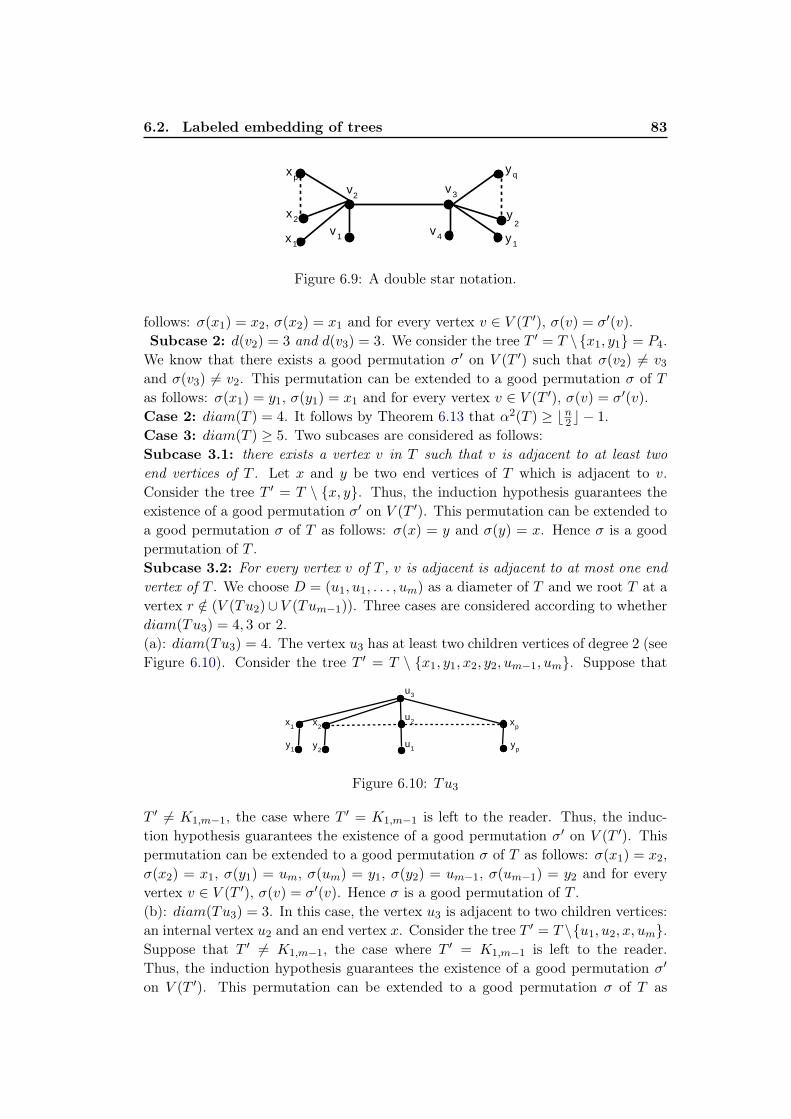
6.2. Labeled embedding of trees 83
v4
v2
v1
v3
x1
xp
y1
yq
x2 y2
Figure 6.9: A double star notation.
follows: σ(x1) = x2, σ(x2) = x1 and for every vertex v ∈ V (T ′), σ(v) = σ′(v).
Subcase 2: d(v2) = 3 and d(v3) = 3. We consider the tree T ′ = T \{x1, y1} = P4.
We know that there exists a good permutation σ′ on V (T ′) such that σ(v2) 6= v3and σ(v3) 6= v2. This permutation can be extended to a good permutation σ of T
as follows: σ(x1) = y1, σ(y1) = x1 and for every vertex v ∈ V (T ′), σ(v) = σ′(v).
Case 2: diam(T ) = 4. It follows by Theorem 6.13 that α2(T ) ≥ ⌊n2 ⌋ − 1.
Case 3: diam(T ) ≥ 5. Two subcases are considered as follows:
Subcase 3.1: there exists a vertex v in T such that v is adjacent to at least twoend vertices of T . Let x and y be two end vertices of T which is adjacent to v.
Consider the tree T ′ = T \ {x, y}. Thus, the induction hypothesis guarantees the
existence of a good permutation σ′ on V (T ′). This permutation can be extended to
a good permutation σ of T as follows: σ(x) = y and σ(y) = x. Hence σ is a good
permutation of T .
Subcase 3.2: For every vertex v of T , v is adjacent is adjacent to at most one endvertex of T . We choose D = (u1, u1, . . . , um) as a diameter of T and we root T at a
vertex r /∈ (V (Tu2)∪ V (Tum−1)). Three cases are considered according to whether
diam(Tu3) = 4, 3 or 2.
(a): diam(Tu3) = 4. The vertex u3 has at least two children vertices of degree 2 (see
Figure 6.10). Consider the tree T ′ = T \ {x1, y1, x2, y2, um−1, um}. Suppose that
x1
u3
u2
u1y1
x2
y2
xp
yp
Figure 6.10: Tu3
T ′ 6= K1,m−1, the case where T ′ = K1,m−1 is left to the reader. Thus, the induc-
tion hypothesis guarantees the existence of a good permutation σ′ on V (T ′). This
permutation can be extended to a good permutation σ of T as follows: σ(x1) = x2,
σ(x2) = x1, σ(y1) = um, σ(um) = y1, σ(y2) = um−1, σ(um−1) = y2 and for every
vertex v ∈ V (T ′), σ(v) = σ′(v). Hence σ is a good permutation of T .
(b): diam(Tu3) = 3. In this case, the vertex u3 is adjacent to two children vertices:
an internal vertex u2 and an end vertex x. Consider the tree T ′ = T \{u1, u2, x, um}.
Suppose that T ′ 6= K1,m−1, the case where T ′ = K1,m−1 is left to the reader.
Thus, the induction hypothesis guarantees the existence of a good permutation σ′
on V (T ′). This permutation can be extended to a good permutation σ of T as
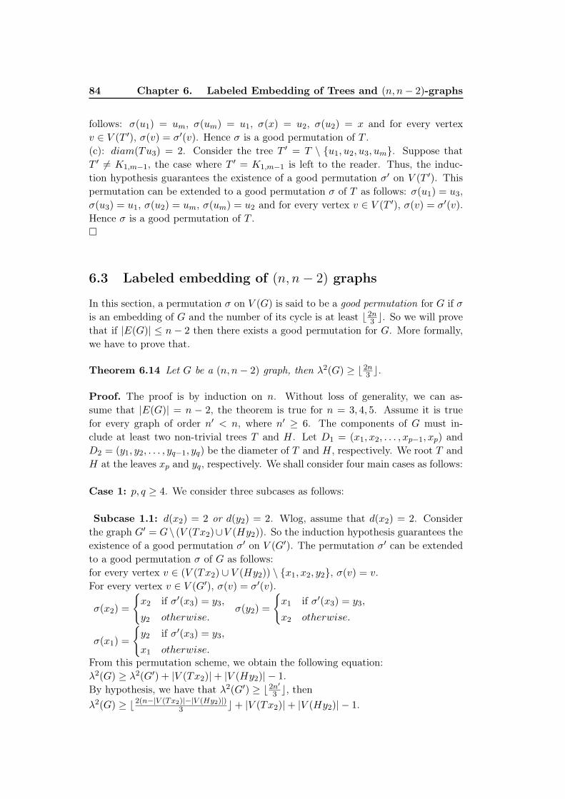
84 Chapter 6. Labeled Embedding of Trees and (n, n− 2)-graphs
follows: σ(u1) = um, σ(um) = u1, σ(x) = u2, σ(u2) = x and for every vertex
v ∈ V (T ′), σ(v) = σ′(v). Hence σ is a good permutation of T .
(c): diam(Tu3) = 2. Consider the tree T ′ = T \ {u1, u2, u3, um}. Suppose that
T ′ 6= K1,m−1, the case where T ′ = K1,m−1 is left to the reader. Thus, the induc-
tion hypothesis guarantees the existence of a good permutation σ′ on V (T ′). This
permutation can be extended to a good permutation σ of T as follows: σ(u1) = u3,
σ(u3) = u1, σ(u2) = um, σ(um) = u2 and for every vertex v ∈ V (T ′), σ(v) = σ′(v).
Hence σ is a good permutation of T .
�
6.3 Labeled embedding of (n, n− 2) graphs
In this section, a permutation σ on V (G) is said to be a good permutation for G if σ
is an embedding of G and the number of its cycle is at least ⌊2n3 ⌋. So we will prove
that if |E(G)| ≤ n− 2 then there exists a good permutation for G. More formally,
we have to prove that.
Theorem 6.14 Let G be a (n, n− 2) graph, then λ2(G) ≥ ⌊2n3 ⌋.
Proof. The proof is by induction on n. Without loss of generality, we can as-
sume that |E(G)| = n − 2, the theorem is true for n = 3, 4, 5. Assume it is true
for every graph of order n′ < n, where n′ ≥ 6. The components of G must in-
clude at least two non-trivial trees T and H. Let D1 = (x1, x2, . . . , xp−1, xp) and
D2 = (y1, y2, . . . , yq−1, yq) be the diameter of T and H, respectively. We root T and
H at the leaves xp and yq, respectively. We shall consider four main cases as follows:
Case 1: p, q ≥ 4. We consider three subcases as follows:
Subcase 1.1: d(x2) = 2 or d(y2) = 2. Wlog, assume that d(x2) = 2. Consider
the graph G′ = G\ (V (Tx2)∪V (Hy2)). So the induction hypothesis guarantees the
existence of a good permutation σ′ on V (G′). The permutation σ′ can be extended
to a good permutation σ of G as follows:
for every vertex v ∈ (V (Tx2) ∪ V (Hy2)) \ {x1, x2, y2}, σ(v) = v.
For every vertex v ∈ V (G′), σ(v) = σ′(v).
σ(x2) =
{
x2 if σ′(x3) = y3,
y2 otherwise.σ(y2) =
{
x1 if σ′(x3) = y3,
x2 otherwise.
σ(x1) =
{
y2 if σ′(x3) = y3,
x1 otherwise.From this permutation scheme, we obtain the following equation:
λ2(G) ≥ λ2(G′) + |V (Tx2)|+ |V (Hy2)| − 1.
By hypothesis, we have that λ2(G′) ≥ ⌊2n′
3 ⌋, then
λ2(G) ≥ ⌊2(n−|V (Tx2)|−|V (Hy2)|)3 ⌋+ |V (Tx2)|+ |V (Hy2)| − 1.
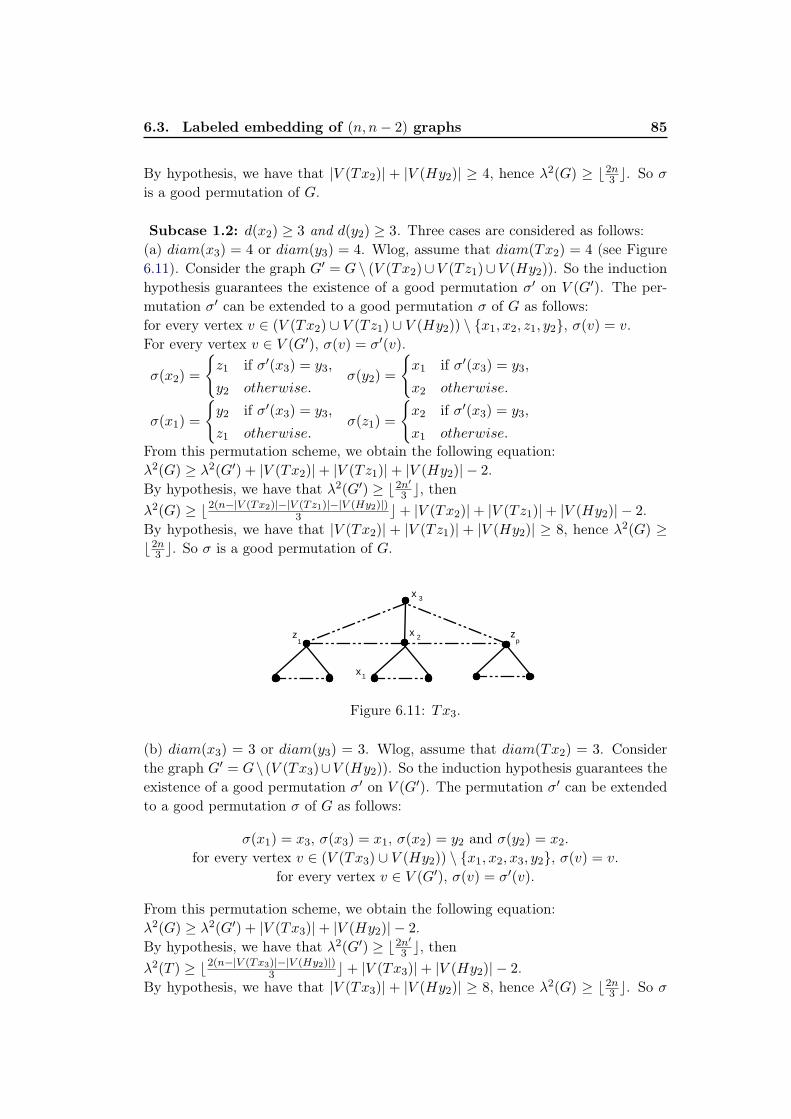
6.3. Labeled embedding of (n, n− 2) graphs 85
By hypothesis, we have that |V (Tx2)| + |V (Hy2)| ≥ 4, hence λ2(G) ≥ ⌊2n3 ⌋. So σ
is a good permutation of G.
Subcase 1.2: d(x2) ≥ 3 and d(y2) ≥ 3. Three cases are considered as follows:
(a) diam(x3) = 4 or diam(y3) = 4. Wlog, assume that diam(Tx2) = 4 (see Figure
6.11). Consider the graph G′ = G \ (V (Tx2)∪ V (Tz1)∪ V (Hy2)). So the induction
hypothesis guarantees the existence of a good permutation σ′ on V (G′). The per-
mutation σ′ can be extended to a good permutation σ of G as follows:
for every vertex v ∈ (V (Tx2) ∪ V (Tz1) ∪ V (Hy2)) \ {x1, x2, z1, y2}, σ(v) = v.
For every vertex v ∈ V (G′), σ(v) = σ′(v).
σ(x2) =
{
z1 if σ′(x3) = y3,
y2 otherwise.σ(y2) =
{
x1 if σ′(x3) = y3,
x2 otherwise.
σ(x1) =
{
y2 if σ′(x3) = y3,
z1 otherwise.σ(z1) =
{
x2 if σ′(x3) = y3,
x1 otherwise.
From this permutation scheme, we obtain the following equation:
λ2(G) ≥ λ2(G′) + |V (Tx2)|+ |V (Tz1)|+ |V (Hy2)| − 2.
By hypothesis, we have that λ2(G′) ≥ ⌊2n′
3 ⌋, then
λ2(G) ≥ ⌊2(n−|V (Tx2)|−|V (Tz1)|−|V (Hy2)|)3 ⌋+ |V (Tx2)|+ |V (Tz1)|+ |V (Hy2)| − 2.
By hypothesis, we have that |V (Tx2)| + |V (Tz1)| + |V (Hy2)| ≥ 8, hence λ2(G) ≥
⌊2n3 ⌋. So σ is a good permutation of G.
x 3
x 2
x1
z1
zp
Figure 6.11: Tx3.
(b) diam(x3) = 3 or diam(y3) = 3. Wlog, assume that diam(Tx2) = 3. Consider
the graph G′ = G\ (V (Tx3)∪V (Hy2)). So the induction hypothesis guarantees the
existence of a good permutation σ′ on V (G′). The permutation σ′ can be extended
to a good permutation σ of G as follows:
σ(x1) = x3, σ(x3) = x1, σ(x2) = y2 and σ(y2) = x2.
for every vertex v ∈ (V (Tx3) ∪ V (Hy2)) \ {x1, x2, x3, y2}, σ(v) = v.
for every vertex v ∈ V (G′), σ(v) = σ′(v).
From this permutation scheme, we obtain the following equation:
λ2(G) ≥ λ2(G′) + |V (Tx3)|+ |V (Hy2)| − 2.
By hypothesis, we have that λ2(G′) ≥ ⌊2n′
3 ⌋, then
λ2(T ) ≥ ⌊2(n−|V (Tx3)|−|V (Hy2)|)3 ⌋+ |V (Tx3)|+ |V (Hy2)| − 2.
By hypothesis, we have that |V (Tx3)| + |V (Hy2)| ≥ 8, hence λ2(G) ≥ ⌊2n3 ⌋. So σ
86 Chapter 6. Labeled Embedding of Trees and (n, n− 2)-graphs
is a good permutation of G.
(c) diam(x3) = 2 and diam(y3) = 2. consider the graph G′ = G\(V (Tx3)∪V (Hy3)).
So the induction hypothesis guarantees the existence of a good permutation σ′ on
V (G′). The permutation σ′ can be extended to a good permutation σ of G as
follows:
σ(x3) = y1, σ(y1) = x3, σ(x1) = y3 and σ(y3) = x1.
for every vertex v ∈ (V (Tx3) ∪ V (Hy3)) \ {x1, x3, y1, y3}, σ(v) = v.
for every vertex v ∈ V (G′), σ(v) = σ′(v).
From this permutation scheme, we obtain the following equation:
λ2(G) ≥ λ2(G′) + |V (Tx3)|+ |V (Hy3)| − 2.
By hypothesis, we have that λ2(G′) ≥ ⌊2n′
3 ⌋, then
λ2(G) ≥ ⌊2(n−|V (Tx3)|−|V (Hy3)|)3 ⌋+ |V (Tx3)|+ |V (Hy3)| − 2.
By hypothesis, we have that |V (Tx3)| + |V (Hy3)| ≥ 8, hence λ2(G) ≥ ⌊2n3 ⌋. So σ
is a good permutation of G.
Case 2: (p = 3 and q ≥ 3) or (p ≥ 3 and q = 3). Wlog, assume that p = 3. Two
subcases are considered as follows:
Subcase 2.1: d(x2) = 2 or d(y2) = 2. This case follows easily using the same
induction scheme as in Subcase 1.1.
Subcase 2.2: d(x2) ≥ 3 and d(y2) ≥ 3. Consider the graph G′ = G\ (T ∪{y1, y2}).
So the induction hypothesis guarantees the existence of a good permutation σ′ on
V (G′). The permutation σ′ can be extended to a good permutation σ of G as
follows:
σ(x3) = x1, σ(x1) = x3, σ(x2) = y2 and σ(y2) = x2.
for every vertex v ∈ V (T ) \ {x1, x2, x3, y1, y2}, σ(v) = v.
for every vertex v ∈ V (G′), σ(v) = σ′(v).
From this permutation scheme, we obtain the following equation:
λ2(G) ≥ λ2(G′) + |V (T )|.
By hypothesis, we have that λ2(G′) ≥ ⌊2n′
3 ⌋, then
λ2(G) ≥ ⌊2(n−|V (T )|−2)3 ⌋+ |V (T )|.
By hypothesis, we have that |V (T )| ≥ 5, hence λ2(G) ≥ ⌊2n3 ⌋. So σ is a good
permutation of G.
Case 3: G has a star Sm. Let v be the root vertex of Sm and let u 6= v be a vertex
of degree 2 of G. Consider the graph G′ = G \ (V (Sm) ∪ {u}). Then there exists a
good permutation for G′, say σ′. Putting σ(u) = v, σ(v) = u, for every leaf vertex
x ∈ V (Sm), σ(x) = x and for x ∈ V (G′), σ(x) = σ′(x) we get a good permutaion
for G.
6.4. Conclusion 87
Case 4: all previous cases are not satisfied. In this case G contains only isolated
vertices (at least two) and non-tree components. Two subcases are considered as
follows:
Subcase 4.1: G has a vertex x of degree at least 3. Let u, v be two isolated vertices
of G. Consider the graph G′ = G \ {u, v, x}). Then there exists a good permuta-
tion for G′, say σ′. Putting σ(u) = u, σ(v) = x, σ(x) = v and for y ∈ V (G′),
σ(y) = σ′(y) we get a good permutaion for G.
Subcase 4.2: all the components of G are cycles and isolated vertices. In this case
we can easily show that G has a good permutation.
From the proof above, we can conclude that λ2(G) ≥ ⌊2n3 ⌋. �
To improve Theorem 6.14, we propose the following conjecture which is probably
true but it seems difficult to prove it!
Conjecture 6.15 Let G be a graph of order n, if |E(G)| ≤ n− 2, then
λ2(G) ≥ ⌊3n
4⌋ − 2
6.4 Conclusion
In this chapter, we have studied the labeled embedding of trees and (n, n−2) graphs.
In particular, we have proved the exact value of the labeled embedding number of
paths and caterpillars. We have also shown the interest to study the fixed-point-free
labeled embedding in order to improve the lower bound of the labeled embedding
number of general trees and (n, n− 2) graphs.
We end this part by reflecting on the applicability of labeled packing to the
graph matching problem. If we consider the example of XML documents that are
modeled as ordered labeled trees, we can see that querying an XML document is
equivalent to searching an embedding of the query in the data tree. Therefore,
it would be interesting to exploit tree embedding techniques in order to define a
coherent similarity measure between two labeled trees. The XML pattern matching
is the subject of the next part of this thesis.

Part III
XML Tree Pattern Matching
Problem

Chapter 7
Tree Matching and XML Retrieval
Contents
7.1 Querying XML Data: Key points . . . . . . . . . . . . . . . . 92
7.1.1 Tree representation of XML documents . . . . . . . . . . . . 92
7.1.2 Query languages . . . . . . . . . . . . . . . . . . . . . . . . . 94
7.2 Algorithms for exact tree pattern matching . . . . . . . . . 96
7.2.1 Notation and terminology . . . . . . . . . . . . . . . . . . . . 96
7.2.2 Algorithms . . . . . . . . . . . . . . . . . . . . . . . . . . . . 96
7.3 Exact tree pattern matching for XML retrieval . . . . . . . 98
7.3.1 Structural join approaches . . . . . . . . . . . . . . . . . . . . 98
7.3.2 Holistic twig join approaches . . . . . . . . . . . . . . . . . . 99
7.3.3 Sequence matching approaches . . . . . . . . . . . . . . . . . 102
7.3.4 Other important exact XML tree algorithms . . . . . . . . . 103
7.3.5 Summary . . . . . . . . . . . . . . . . . . . . . . . . . . . . . 104
7.4 Conclusion . . . . . . . . . . . . . . . . . . . . . . . . . . . . . 104
Among all the available formats used to represent information (from text to
video or audio), the XML (eXtensible Markup Language) [W3C98b] format is now
extensively used. The simple, self-description nature of the XML standard promises
to enable a broad suite of next-generation Internet applications, ranging from intel-
ligence Web searching and querying to e-commerce.
The growing number of XML documents leads to the need for appropriate re-
trieval methods which are able to exploit the specific features of this type of
documents. Indeed, in XML documents, textual content (data) is hierarchically
structured with tags. As opposed to other markup languages (like HTML for ex-
ample), tags are used to specify semantic information about the content, and not
for presentation purposes. Although structure allows to organize content in XML
documents, it is not always used with the same intent. XML documents can be
either data-oriented, where structure is intensively used to organize data, and
where XML components can be seen as database records, or text-oriented, where
structure is irregular and documents are designed to be used by humans.
Many approaches have been proposed in the literature for XML retrieval. How-
ever, most of them propose ab nihilo solutions, whereas the use of graph theoretical
92 Chapter 7. Tree Matching and XML Retrieval
concepts could be of interest. Indeed, the underlying data model of XML docu-
ments allows to consider them as a particular kind of graphs, i.e., trees [W3C98a].
More precisely, they can be considered as labeled trees of element nodes, where each
element can be either an atomic data item or a composite data collection consisting
of references (represented as edges) to child elements in the XML tree. The same
representation can be used for structured queries. Considering this data model for
retrieval, the retrieval process can thus be seen as a matching problem between
query and document trees.
In this chapter, we aim at studying and discussing what are the solutions pro-
posed by graph theory for the tree-matching problem in a general perspective, and
how they have been exploited in XML retrieval. In particular, we will focus our
attention on the exact tree matching problem.
7.1 Querying XML Data: Key points
Before giving some algorithms used in graph theory for tree matching, it seems
of great importance to recall some background about XML documents and query
languages, and to detail issues behind the retrieval of XML information.
7.1.1 Tree representation of XML documents
In XML documents, tags are used to hierarchically and semantically organize infor-
mation. In the document presented in Figure 7.1 for example, content is organized
within a header and a body tag. The body tag contains section elements, which are
in turn composed of title and paragraph elements, etc.
An element begins with an opening tag <tag> and ends with a closing tag
</tag>. It may contain atomic data (as for example author element), other ele-
ments (as for example one of the section elements) or a mixture of both (one talk
about mixed content). Elements are also called components.
Thanks to this data model, XML documents can be represented as labeled trees
[W3C98a]. In an XML tree, the whole document is represented by the root node,elements are represented by internal nodes (i.e., non terminal nodes) and the con-
tent itself is in leaf nodes (i.e., terminal nodes). These nodes are linked with edges
showing their hierarchical relations. The tree representation of the document in
Figure 7.1 is given in Figure 7.2.
As previously mentioned, XML documents can be classified into two groups of
documents: data-oriented documents or text-oriented documentsDocuments of the first category have a fine granularity, are highly structured and
do not contain mixed contents. The order of the children of a given element is often
without any importance. Elements can be considered as database records, there are
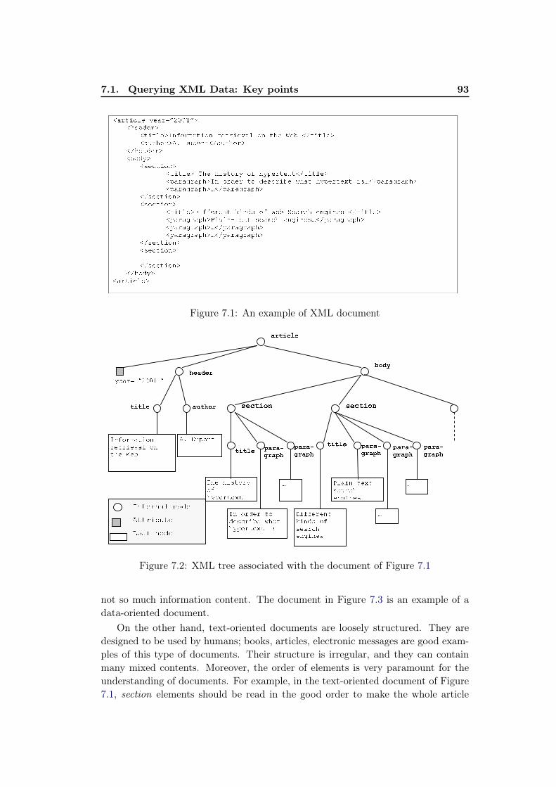
7.1. Querying XML Data: Key points 93
�✁✂✄☎✆✝✞ ✟✞✁✂✠✡☛☞☞✌✡✍
�✎✞✁✏✞✂✍
�✄☎✄✝✞✍✑✒✓✔✂✕✁✄☎✔✒ ✂✞✄✂☎✞✖✁✝ ✔✒ ✄✎✞ ✗✞✘ �✙✄☎✄✝✞✍
�✁✚✄✎✔✂✍✛✜ ✢✚✣✔✒✄�✙✁✚✄✎✔✂✍
�✙✎✞✁✏✞✂✍
�✘✔✏✟✍
�✤✞✆✄☎✔✒✍
�✄☎✄✝✞✍ ✥✎✞ ✎☎✤✄✔✂✟ ✔✓ ✎✟✣✞✂✄✞✦✄�✙✄☎✄✝✞✍
�✣✁✂✁✧✂✁✣✎✍✑✒ ✔✂✏✞✂ ✄✔ ✏✞✤✆✂☎✘✞ ★✎✁✄ ✎✟✣✞✂✄✞✦✄ ☎✤✩�✙✣✁✂✁✧✂✁✣✎✍
�✣✁✂✁✧✂✁✣✎✍✩�✙✣✁✂✁✧✂✁✣✎✍
�✙✤✞✆✄☎✔✒✍
�✤✞✆✄☎✔✒✍
�✄☎✄✝✞✍✢☎✓✓✞✂✞✒✄ ✪☎✒✏✤ ✔✓ ✗✞✘ ✫✞✁✂✆✎ ✞✒✧☎✒✞✤ �✙✄☎✄✝✞✍
�✣✁✂✁✧✂✁✣✎✍✬✝✁☎✒✭✄✞✦✄ ✤✞✁✂✆✎ ✞✒✧☎✒✞✤✩�✙✣✁✂✁✧✂✁✣✎✍
�✣✁✂✁✧✂✁✣✎✍✩�✙✣✁✂✁✧✂✁✣✎✍
�✣✁✂✁✧✂✁✣✎✍✩�✙✣✁✂✁✧✂✁✣✎✍
�✙✤✞✆✄☎✔✒✍
�✤✞✆✄☎✔✒✍
✩
�✙✤✞✆✄☎✔✒✍
�✙✘✔✏✟✍
�✁✂✄☎✆✝✞✍
Figure 7.1: An example of XML document
�✁✂✄☎✆✝✞✟✄✁
☎✠✞☎✟✠✡✝☛ ✄✁
✞☞✠ ✌✠✍
✖✠✝☎✗ ✘✙✙✚
✧☞✠ ☞✟★✞✄☎✖
✄✂
�✁ ✄☎✪✠☎ ✞✄
✪✠★✫☎✟✍✠ ✬☞✝✞
☞✖✦✠☎✞✠✩✞ ✟★
✤✟✂✂✠☎✠✁✞
✭✟✁✪★ ✄✂
★✠✝☎✫☞
✠✁✮✟✁✠★
✰☛✝✟✁✱✞✠✩✞
★✠✝☎✫☞
✿✏✎✽✛
❀❁❂❃❄❁❅❆ ❁❇❈❃
❉❂❂❄❊❋●❂❃
❍❃❅■ ❁❇❈❃
✿✏✎✽✛ ✿✏✎✽✛ ✿✏✎✽✛ ✿✏✎✽✛
Figure 7.2: XML tree associated with the document of Figure 7.1
not so much information content. The document in Figure 7.3 is an example of a
data-oriented document.
On the other hand, text-oriented documents are loosely structured. They are
designed to be used by humans; books, articles, electronic messages are good exam-
ples of this type of documents. Their structure is irregular, and they can contain
many mixed contents. Moreover, the order of elements is very paramount for the
understanding of documents. For example, in the text-oriented document of Figure
7.1, section elements should be read in the good order to make the whole article
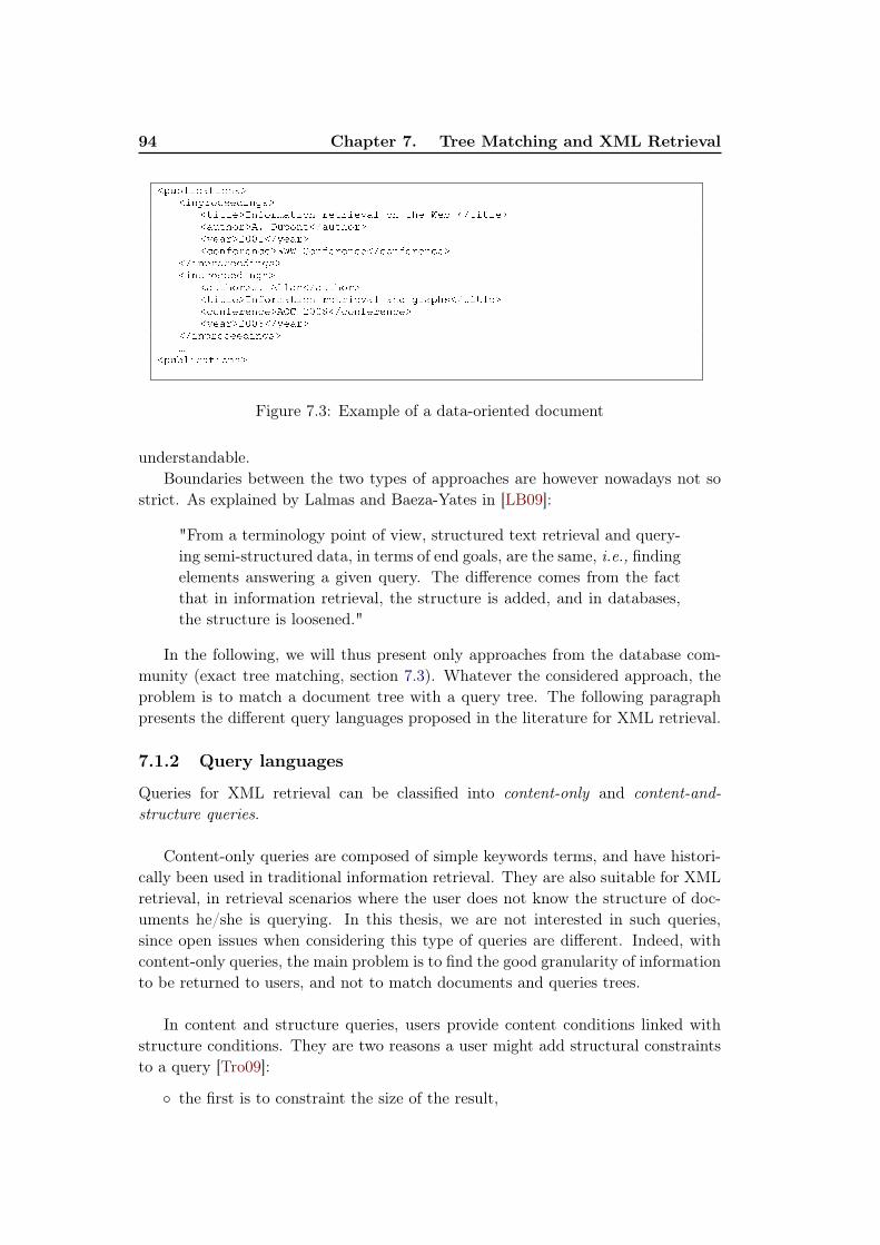
94 Chapter 7. Tree Matching and XML Retrieval
�✁✂✄☎✆✝✞✟✆✠✡☛☞
�✆✡✁✌✠✝✍✍✎✆✡✏☛☞
�✟✆✟☎✍☞✑✡✒✠✌✓✞✟✆✠✡ ✌✍✟✌✆✍✔✞☎ ✠✡ ✟✕✍ ✖✍✄ �✗✟✆✟☎✍☞
�✞✂✟✕✠✌☞✘✙ ✚✂✁✠✡✟�✗✞✂✟✕✠✌☞
�✛✍✞✌☞✜✢✢✣�✗✛✍✞✌☞
�✝✠✡✒✍✌✍✡✝✍☞✖✖✖ ✤✠✡✒✍✌✍✡✝✍�✗✝✠✡✒✍✌✍✡✝✍☞
�✗✆✡✁✌✠✝✍✍✎✆✡✏☛☞
�✆✡✁✌✠✝✍✍✎✆✡✏☛☞
�✞✂✟✕✠✌☞✥✙ ✘☎☎✞✡�✗✞✂✟✕✠✌☞
�✟✆✟☎✍☞✑✡✒✠✌✓✞✟✆✠✡ ✌✍✟✌✆✍✔✞☎ ✞✡✎ ✏✌✞✁✕☛�✗✟✆✟☎✍☞
�✝✠✡✒✍✌✍✡✝✍☞✘✦✤ ✜✢✢✧�✗✝✠✡✒✍✌✍✡✝✍☞
�✛✍✞✌☞✜✢✢✧�✗✛✍✞✌☞
�✗✆✡✁✌✠✝✍✍✎✆✡✏☛☞
★
�✁✂✄☎✆✝✞✟✆✠✡☛☞
Figure 7.3: Example of a data-oriented document
understandable.
Boundaries between the two types of approaches are however nowadays not so
strict. As explained by Lalmas and Baeza-Yates in [LB09]:
"From a terminology point of view, structured text retrieval and query-
ing semi-structured data, in terms of end goals, are the same, i.e., finding
elements answering a given query. The difference comes from the fact
that in information retrieval, the structure is added, and in databases,
the structure is loosened."
In the following, we will thus present only approaches from the database com-
munity (exact tree matching, section 7.3). Whatever the considered approach, the
problem is to match a document tree with a query tree. The following paragraph
presents the different query languages proposed in the literature for XML retrieval.
7.1.2 Query languages
Queries for XML retrieval can be classified into content-only and content-and-structure queries.
Content-only queries are composed of simple keywords terms, and have histori-
cally been used in traditional information retrieval. They are also suitable for XML
retrieval, in retrieval scenarios where the user does not know the structure of doc-
uments he/she is querying. In this thesis, we are not interested in such queries,
since open issues when considering this type of queries are different. Indeed, with
content-only queries, the main problem is to find the good granularity of information
to be returned to users, and not to match documents and queries trees.
In content and structure queries, users provide content conditions linked with
structure conditions. They are two reasons a user might add structural constraints
to a query [Tro09]:
◦ the first is to constraint the size of the result,
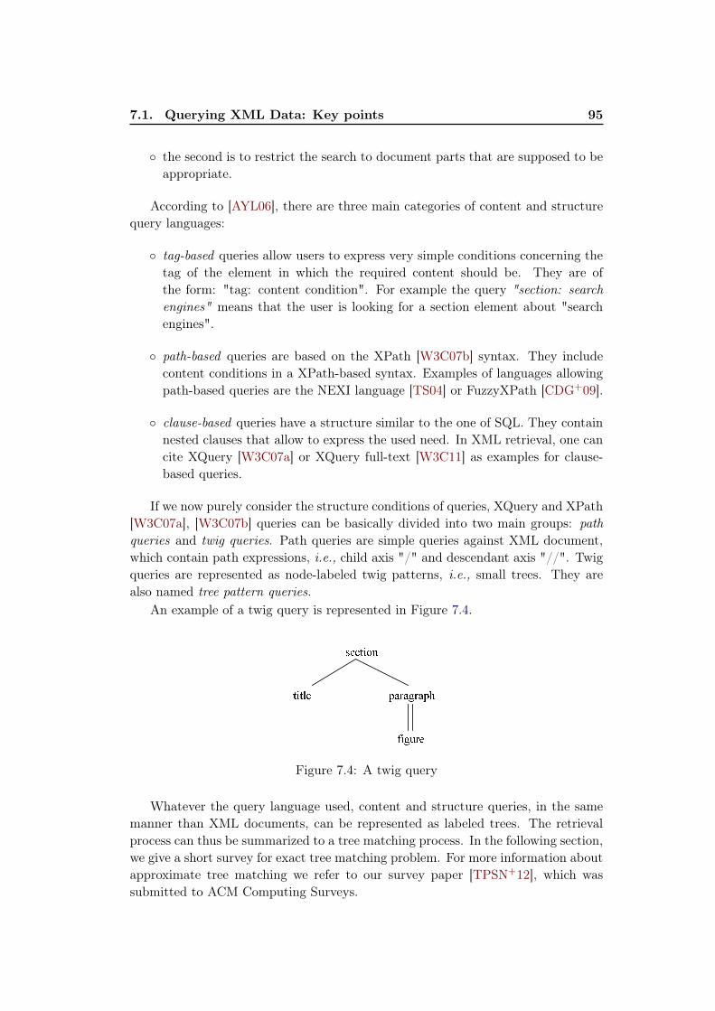
7.1. Querying XML Data: Key points 95
◦ the second is to restrict the search to document parts that are supposed to be
appropriate.
According to [AYL06], there are three main categories of content and structure
query languages:
◦ tag-based queries allow users to express very simple conditions concerning the
tag of the element in which the required content should be. They are of
the form: "tag: content condition". For example the query "section: searchengines" means that the user is looking for a section element about "search
engines".
◦ path-based queries are based on the XPath [W3C07b] syntax. They include
content conditions in a XPath-based syntax. Examples of languages allowing
path-based queries are the NEXI language [TS04] or FuzzyXPath [CDG+09].
◦ clause-based queries have a structure similar to the one of SQL. They contain
nested clauses that allow to express the used need. In XML retrieval, one can
cite XQuery [W3C07a] or XQuery full-text [W3C11] as examples for clause-
based queries.
If we now purely consider the structure conditions of queries, XQuery and XPath
[W3C07a], [W3C07b] queries can be basically divided into two main groups: pathqueries and twig queries. Path queries are simple queries against XML document,
which contain path expressions, i.e., child axis "/" and descendant axis "//". Twig
queries are represented as node-labeled twig patterns, i.e., small trees. They are
also named tree pattern queries.An example of a twig query is represented in Figure 7.4.
Figure 7.4: A twig query
Whatever the query language used, content and structure queries, in the same
manner than XML documents, can be represented as labeled trees. The retrieval
process can thus be summarized to a tree matching process. In the following section,
we give a short survey for exact tree matching problem. For more information about
approximate tree matching we refer to our survey paper [TPSN+12], which was
submitted to ACM Computing Surveys.
96 Chapter 7. Tree Matching and XML Retrieval
7.2 Algorithms for exact tree pattern matching
This section describes state-of-the-art algorithms for exact tree matching. In order
to state the problem, the terminology of labeled tree and their components has to
be defined first.
7.2.1 Notation and terminology
A rooted labeled tree is denoted by T = (V,E, r, µ), where V = {v1, v2, . . . , vn}
is a finite set of nodes, E ⊆ {(u, v)|u, v ∈ V } is a set of edges. The node r is a
distinguished node called the root, and µ is a labeling function which maps each
node of T to a label in a finite set L = {l1, l2, ..., lk}. For brevity, in the remaining
of this chapter, we call a rooted labeled tree simply a tree. We denote the level
of a vertex v by l(v). We recall that an ordered tree is a rooted tree for which an
ordering is specified for the children of every node, and it is unordered otherwise.
We give below the formal definition of the exact tree matching problem.
Definition 7.1 Let target T1 = (V1, E1, r1, µ1) and pattern T2 = (V2, E2, r2, µ2) betwo ordered labeled trees. T2 matches T1 at node x1 6= r1 if there exists a one-to-oneinjective function from the nodes of T2 into the nodes of T1 such that:
1. the root of T2 maps to x1,
2. if v2 ∈ V2 maps to v1 ∈ V1, then µ1(v1) = µ2(v2),
3. if v2 ∈ V2 maps to v1 ∈ V1 and v1 is not a leaf, then each child of v2 maps tosome child of v1.
Figure 7.5 shows an example of a tree pattern matching between pattern tree
P and target tree T , where the one-to-one mappings is represented by dotted lines.
The tree pattern matching problem has been largely studied and has many impor-
tant applications such as term rewriting systems, transformational programming
systems, code-generator generators, theorem provers, and a variety of functional
languages with equational function definitions (see [HO82]). The following is a brief
overview of general exact tree pattern matching algorithms.
7.2.2 Algorithms
Given a tree pattern P and a target T of order m and n, respectively, where m ≤ n,
a naive tree pattern matching algorithm takes O(mn) in the worst case. The basic
idea is to visit all nodes of T in a pre-order walk, for each visited node a special
recursive procedure is applied to check for possible occurrence of P at that node v.
The matching procedure is terminated as soon as a mismatch is detected.
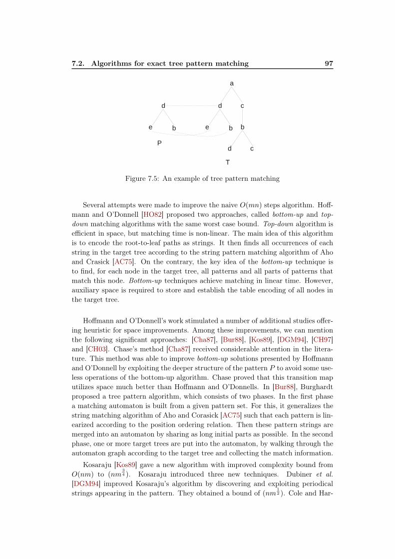
7.2. Algorithms for exact tree pattern matching 97
Figure 7.5: An example of tree pattern matching
Several attempts were made to improve the naive O(mn) steps algorithm. Hoff-
mann and O’Donnell [HO82] proposed two approaches, called bottom-up and top-down matching algorithms with the same worst case bound. Top-down algorithm is
efficient in space, but matching time is non-linear. The main idea of this algorithm
is to encode the root-to-leaf paths as strings. It then finds all occurrences of each
string in the target tree according to the string pattern matching algorithm of Aho
and Crasick [AC75]. On the contrary, the key idea of the bottom-up technique is
to find, for each node in the target tree, all patterns and all parts of patterns that
match this node. Bottom-up techniques achieve matching in linear time. However,
auxiliary space is required to store and establish the table encoding of all nodes in
the target tree.
Hoffmann and O’Donnell’s work stimulated a number of additional studies offer-
ing heuristic for space improvements. Among these improvements, we can mention
the following significant approaches: [Cha87], [Bur88], [Kos89], [DGM94], [CH97]
and [CH03]. Chase’s method [Cha87] received considerable attention in the litera-
ture. This method was able to improve bottom-up solutions presented by Hoffmann
and O’Donnell by exploiting the deeper structure of the pattern P to avoid some use-
less operations of the bottom-up algorithm. Chase proved that this transition map
utilizes space much better than Hoffmann and O’Donnells. In [Bur88], Burghardt
proposed a tree pattern algorithm, which consists of two phases. In the first phase
a matching automaton is built from a given pattern set. For this, it generalizes the
string matching algorithm of Aho and Corasick [AC75] such that each pattern is lin-
earized according to the position ordering relation. Then these pattern strings are
merged into an automaton by sharing as long initial parts as possible. In the second
phase, one or more target trees are put into the automaton, by walking through the
automaton graph according to the target tree and collecting the match information.
Kosaraju [Kos89] gave a new algorithm with improved complexity bound from
O(nm) to (nm34 ). Kosaraju introduced three new techniques. Dubiner et al.
[DGM94] improved Kosaraju’s algorithm by discovering and exploiting periodical
strings appearing in the pattern. They obtained a bound of (nm12 ). Cole and Har-
98 Chapter 7. Tree Matching and XML Retrieval
iharan [CH97] introduced and gave an efficient algorithm for the subset Matchingproblem. The goal of this problem is to find all occurrences of a pattern string P of
length m in a text string T of length n. Then the tree pattern matching has been
reduced to a number of instances of the subset matching problem. Combining this
reduction with the subset matching algorithm take an O(n log3m) time randomized
algorithm for the tree pattern matching problem. Later the same authors improved
the reduction time complexity [CH03]. They obtained an O(n log2m + m) time
deterministic algorithm and an O(n log n+m) time Monte Carlo algorithm for the
tree pattern matching problem.
7.3 Exact tree pattern matching for XML retrieval
As we have seen in Section 7.1, XML uses a tree-structured model for representing
data and twig patterns for expressing queries. Finding all occurrences of such a
twig pattern in an XML database is clearly a core operation in XML query process-
ing. There has been a great deal of interest in recent years to overcome efficiently
this problem. Most of the proposed approaches in the literature are interested in
structural properties of queries and can be classified into four groups:
◦ structural join approaches,
◦ holistic twig join approaches,
◦ sequence matching approaches,
◦ other important exact XML tree matching algorithms.
In the following, we present an overview of the main algorithms and results available
in each group.
7.3.1 Structural join approaches
In this section, we review the join based approach, a very important native
idea, which usually includes three parts: (1) decomposition, (2) matching and (3)
merging. Firstly, a twig pattern is decomposed into a set of basic parent-child and
ancestor-descendant relationships between pairs of nodes. In the second phase, each
binary relationship is separately executed using structural join techniques and its
intermediate results are stored for further processing. The final result is formed by
merging the intermediate results. We describe in the following the two main struc-
tural join algorithms proposed in the literature.
(i) Multi-predicate merge join algorithm
The key to the efficiency of this algorithm is in the use of a containment labelingscheme [ZND+01] that encodes each element in an XML database by its positional
7.3. Exact tree pattern matching for XML retrieval 99
information. The main purpose of this representation is that the structural relation-
ship between two vertices u, v can be determined easily without knowledge of the
intermediate nodes on the path between u, v. For more information, this labeling
scheme (called also region encoding) will be described in detail in the next chapter.
Based on the containment labeling scheme, Zhang et al. [ZND+01] proposed
the multi-predicate merge join (MPMGJN ) algorithm, which is the first structural
join to find all occurrences of the basic structural relationships. This mechanism
is an extension of the classical merge-join algorithm developed in relational query
optimizers for equi-joins. The results of Zhang showed that for many XML queries,
MPMGJN is more than an order-of-magnitude faster than the standard Relational
Database Management System (RDBMS) join implementations.
(ii) Tree-Merge and Stack-Tree algorithm:
Al-Khalifa et al. [AJK+02] took advantage of the containment labeling scheme
of XML elements to decrease the time of join processing. They developed two algo-
rithms for matching parent-child and ancestor-descendant structural relationships
efficiently: Tree-Merge and Tree-Stack.The behavior of these two algorithms is explained by analytical results. In
particular, the Stack-Tree algorithm was shown to be both I/O and CPU optimal,
and practically as efficient as Tree-Merge family for evaluating containment queries.
7.3.2 Holistic twig join approaches
Until now, the holistic twig join approach was regarded as the most efficient
family in the literature. Bruno et al. [BKS02] proposed the first holistic XML twig
pattern matching algorithm to avoid producing large intermediate results. This ap-
proach constituted the major attempt for several subsequent works in order to make
the twig pattern matching very efficient. In the following, we present an overview
of the basic ideas and results of the main holistic twig join algorithms available in
the literature.
(i) TwigStack algorithm
The main disadvantage of twig query decomposition into multiple binary re-
lationships is that this approach generates a large amount of intermediate query
results even when the input and output size are more manageable. Frequently, such
intermediate results cannot be held in main memory and must be stored on disk.
This will result in high disk I/O cost. In order to overcome this weakness, Bruno etal. [BKS02] proposed a novel holistic twig join algorithm, called TwigStack, wherein
no large intermediate results are created.
The idea behind this approach is to use a chain of linked stacks to compactly
represent partial results of individual query root-to-leaf paths, which are then com-
posed to produce the final solutions. This decomposition method avoids computing
100 Chapter 7. Tree Matching and XML Retrieval
large redundant intermediate results. This algorithm will be described in detail in
the next chapter. The main advantage of this approach is to avoid storing interme-
diate results unless they contribute to the final results when the query twig has only
ancestor-descendant edges. The analytical results of this approach demonstrate that
TwigStack is I/O and CPU optimal among all sequential algorithms that read the
entire input. This analysis is confirmed by experimental results on a range of real
synthetic data and query twig patterns. The experimental results suggest that the
holistic approach has more than six-fold faster query processing performance than
the Stack-Tree approach coupled with the optimal join order.
(ii) Improvements on TwigStack
The idea of holistic twig join has been adopted in several works in order to make
the structural join algorithm very efficient. This section is devoted to a structured
review of these advances.
Improvement 1: efficient processing of parent-child edge query. As men-
tioned before, when all edges in query patterns are ancestor-descendant queries,
TwigStack ensures that each root-to-leaf intermediate solution contributes to the
final results. However, this algorithm still cannot control a large number of interme-
diate results for parent-child edge query. In the first improvement attempt, many
efficient algorithms for XML twig pattern have been proposed to efficiently handle
twig queries with parent-child relationships. Among them, Lu et al. [LCL04] ex-
tended TwigStack by proposing TwigStackList algorithm. This algorithm has the
same performance than TwigStack for query patterns with only ancestor-descendant
edges, but also produces much less useless intermediate solutions than TwigStackfor queries with parent-child relationships. The main technique of TwigStackListalgorithm is to look-ahead read more elements in the input streams and saves some
of them (only those that might contribute to final answers) into lists in the main
memory, so that we can make a more accurate decision to determine whether an el-
ement can contribute to the final solution or not. The experimental results obtained
by authors demonstrate the significant superiority of TwigStackList on TwigStackaccording to the size of intermediate results for queries with parent-child edges.
Chen et al. [CLL05] suggested another algorithm, called iTwigJoin, which can be
used on various data streaming strategies (e.g. Tag+Level Streaming and PrefixPath Streaming). Tag+Level streaming can be optimal for both ancestor-descendant
and parent-child only twig patterns whereas Prefix Path streaming could be optimal
for ancestor-descendant only, parent-child relationship only. The experiments in
[CLL05] show that Tag+Level streaming guarantees very few useless intermediate
solutions in most case tested. None of the previous algorithms can avoid useless in-
termediate solutions completely. Li and Wang [LW08b] proposed the first algorithm,
called TwigBuffer that completely avoids the useless partial solutions for arbitrary
twig patterns. TwigBuffer use the same idea of buffering like TwigStackList to
buffers some elements from the input streams in order to check the parent-child
7.3. Exact tree pattern matching for XML retrieval 101
relationships. The experimental results show that TwigStackList and TwigBufferhave the same performance when the queries that do not have parent-child edges
or parent-child edges happen under non-branching nodes. However TwigBuffer per-
forms better than TwigStackList when the queries have parent-child edges under
branching nodes.
Improvement 2: elimination of redundant computations. The existing holis-
tic twig join algorithms may perform many redundant checks of XML elements.
Indeed, an improvement strategy consists in avoiding these unnecessary computa-
tions. TSGeneric+ [JWLY03] makes improvements on TwigStack by using XR-Treeto effectively skip some useless elements that do not contribute to the final results.
The motivation to use XR-tree is that, the ancestors (or descendants) of any XML
element indexed by an XR-tree can be derived with optimal worst case I/O cost.
However, TSGeneric+ may still output many useless intermediate path solutions
like TwigStack for queries with parent-child relationship. Guoliang et al. [LFZZ07]
proposed the TJEssential algorithm based on three optimization rules to avoid some
unnecessary computations. They presented two algorithms incorporated with these
optimization rules to effectively answer twig patterns in leaf-to-root combining with
root-to-leaf way. A novel holistic twig join algorithm, called TwigStack+ is proposed
in [ZXM07], it is based on holistic twig join guided by extended solution extension to
avoid many redundant computations. It significantly improves the query processing
cost, simply because it can check whether other elements can be processed together
with current one.
Improvement 3: eliminate the merging phase. Another improvement con-
sists in reducing the cost of queries execution. Indeed there exist very interest-
ing approaches that eliminate the second phase of merging of individual solutions
[CLT+06], [QYD07], [JLH+07], [LW08a]. However, these algorithms need to load
the entire document tree in memory. Chen et al. [CLT+06] proposed the first tree
pattern solution, called Twig2Stack that avoids any post path join. Twig2Stackalgorithm uses a hierarchical-stack to capture the ancestor-descendant relationships
for the elements in the same query node. In this way, Twig2Stack can process path
matching efficiently without a redundant relationships checking. Twig2Stack algo-
rithm has shown a better performance in query processing than TwigStack and TJ-Fast [LLCC05] (see below). However, maintaining the hierarchical structure among
stacks in Twig2Stack algorithm has a critical impact on the performance processing
of twig query. Aiming to avoid this complex hierarchical-stacks, Qin et al. [QYD07]
proposed an algorithm, called TwigList, which is a refined version of Twig2Stack. In
fact, the main difference between both methods is that TwigList has only changed
the complicated stacks used in Twig2Stack to simple list structures. The experi-
mental studies of Qin et al. [QYD07] show that TwigList algorithm outperforms
Twig2Stack as well as TwigStack. In the same context a novel algorithm, called
HolisticTwigStack was developed in [JLH+07]. The authors proposed a novel com-
plex stack structure like Twig2Stack to preserve the holisticity of the twig matches,
102 Chapter 7. Tree Matching and XML Retrieval
without generating intermediate solutions. However, a considerable amount of time
is taken to maintain the stack structure. HolisticTwigStack were evaluated better
than both TwigStack and Twig2Stack in terms of time complexity, memory space
and I/O. complexity. Dao and Gao [DC08] reviewed and analyzed both of the Holis-ticTwigStack and TwigList algorithm on processing for XML twig pattern matching.
The statistics from this analysis clearly indicate that the TwigList algorithm seems
to be significantly more efficient in the most tested cases.
Improvement 4: benefit the properties of some labeling schemes. Most
of the existing holistic twig join algorithms are based on region encoding scheme
(which will be explained in detail in the following chapter) to capture the struc-
tural relationship between XML elements. However, there exist other approaches
which exploit others labeling scheme. Among them, Dewey labeling scheme has
been widely used in XML query processing. A Dewey label of a node v represents
the path from the document root to v. Based on the Dewey labeling, Lu et al.[LLCC05] proposed TJFast algorithm which uses a new encoding scheme, called the
extended Dewey code, which allows to combine effectively the types and identifiers of
elements in a label. The main advantage of this labeling is that, the ancestors of any
XML element can be derived from its label alone. Thus, TJFast typically access
much less elements than algorithms based on region encoding and can efficiently
process queries with wildcards in internal nodes. More recently, based on the pre-
liminary idea of extended Dewey labeling scheme and TJFast algorithm, Lu et al.[LML11] proposed three novel holistic twig join algorithms GTJFast, TJFastTL and
GTJFastTL. The first algorithm GTJFast allows to compactly represent the inter-
mediate matching solutions and avoid the output of non-return nodes to reduce the
I/O cost. Both TJFastTL and GTJFastTL algorithms are proposed by extending
TJFast and GTJFast algorithm based on tag +level streaming scheme. In tag +levelstreaming, XML elements with the same label but different level numbers have been
separated to different streams. This level information is used to prune some useless
streams. The authors proved that TJFastTL and GTJFastTL guarantee the I/O op-
timality for queries with only parent-child relationships. The experimental results
reported in [LML11] show that these algorithms are superior to existing approaches
in terms of the number of scanned elements, the size of intermediate solutions and
query performance.
7.3.3 Sequence matching approaches
As opposed to the holistic twig join algorithm, the sequence matching approaches
use an indexing method to transform both XML documents and queries into se-
quences and evaluate queries based on sequence matching. Querying XML data is
equivalent to find subsequence matches. In [ZMM04] and [ZADR03], the authors
use the pre-order and post-order ranks to linearize the tree structures and apply
the sequence inclusion algorithms for strings. They proposed a novel strategy that
include three parts. Firstly, a query decomposition process is applied to transform

7.3. Exact tree pattern matching for XML retrieval 103
the query twig into a set of root-to-leaf paths so that the ordered tree inclusion can
be safely applied. It has to be evaluated against the data signature in the second
phase. Finally, the set of answers is determined by joining compatible intermediate
solutions. The experiments in [ZADR03] demonstrate the efficiency of the decom-
position approach, which is especially advantages for the large query trees, and for
trees with highly selective predicates.
Two other sequence matching algorithms, ViST [WPFY03] and PRIX [RM04]
were proposed to avoid expensive join operations. ViST method represents a major
departure from previous XML indexing approaches. In fact, unlike classical index
methods that decompose a query into multiple sub-queries, and then join the solu-
tions of these sub-queries to provide the final answers, ViST uses tree structures as
the basic unit of query to avoid expensive join operations. This method introduced
a new sequential representation that transforms XML data trees and twig queries
into structure-encoded sequences. ViST performs efficient subsequence matching
algorithms on the structure-encoded sequences to find twig patterns in XML doc-
uments. However, the query processing in ViST may result in false alarms and
false dismissals (these two problems are explained in more detail in [WM05]). In
[RM04], Rao and Moon proposed a new indexing XML documents and process-
ing twig patterns in an XML database. This indexing approach transforms XML
documents and twig query into sequences by prüfer method that constructs an one-
to-one correspondence between trees and sequences. Based on this transformation,
a query execution system, called PRIX (Prüfer sequences for indexing XML) is
developed for indexing XML documents and processing twig queries. The matching
phase is achieved by applying subsequence matching on the set of sequences in XML
database.
7.3.4 Other important exact XML tree algorithms
In this section, we take a quick look over some other well-known query tree
pattern processing algorithms which have been developed in recent years. Among
them, some approaches have benefited from fundamental progress in node labeling
schemes of XML documents (for a survey, see [HL09]).
In [WL08], a twig pattern matching algorithm, called TwigVersion is proposed.
the key idea of this approach is to compress both structural index and number-
ing schemes technique. TwigVersion is based on new version-labeling scheme that
encodes all repetitive structures in XML documents. The identification of these
repetitive structures matching allows to avoid a large amount of unnecessary com-
putations. The experimental results reported in [WL08] show that TwigVersionsignificantly outperforms TwigStack, TJFast and Twig2Stack algorithms.
Recently, Izadi et al. [IHH09] proposed a novel method, called S3, which can
selectively process the document nodes. In S3, unlike all previous methods, path ex-
104 Chapter 7. Tree Matching and XML Retrieval
pressions are not directly executed on the XML document, but they first evaluated
against a guidance structure, called QueryGuide. The information extracted from
the QueryGuide is an abstraction of the XML document. It describes the struc-
ture of XML document by its paths, such as the nodes of XML data are labeled
by Dewey labeling scheme. The experimental results of [IHH09] confirm that S3
substantially outperforms TwigStack , TJFast, and TwigList in terms of response
time, I/O overhead, and memory consumption-critical parameters.
7.3.5 Summary
Table 7.1 depicts the various approaches presented in this section. These approaches
are categorized into four classes by considering three basic features: the decompo-
sition technique, the labeling technique, and a boolean parameter which indicates
whether the merging phase is used in the query processing or not.
7.4 Conclusion
Much research effort has been devoted on efficient XML query processing. As a core
operation in XML data, finding all occurrences of a query pattern in XML docu-
ments attracted more and more attention. In this chapter, we gave a structured
overview of the numerous recent advances in the exact tree matching for querying
XML data. As mentioned before, a very large volume of algorithms were proposed
in the literature, and it seems nearly impossible to consider all related works. It is
however difficult to decide what is the best algorithm that performs the query pro-
cessing efficiently. For example, the one-phase holistic twig join algorithm eliminates
completely the second phase of merging at the expense of huge memory requirement.
Of course, holistic twig join algorithms are good candidates for physical operators
supporting query evaluation in XDBMSs. Therefore, the development of new struc-
tural join algorithms is still valuable, the next chapter follows this line of research,
In particular, we will propose a new efficient holistic twig join algorithm, called
TwigStack++, which can greatly improves query processing performance of XML
documents.
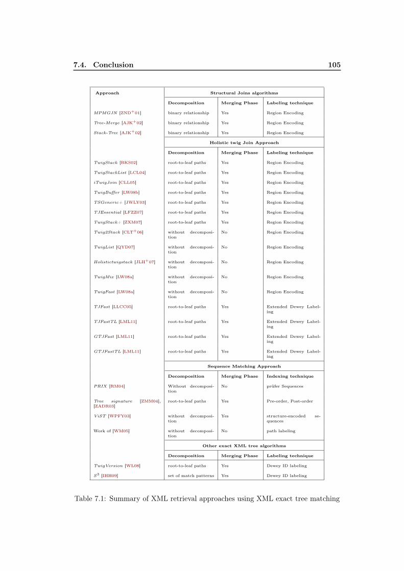
7.4. Conclusion 105
Approach Structural Joins algorithms
Decomposition Merging Phase Labeling technique
MPMGJN [ZND+01] binary relationship Yes Region Encoding
Tree-Merge [AJK+02] binary relationship Yes Region Encoding
Stack-Tree [AJK+02] binary relationship Yes Region Encoding
Holistic twig Join Approach
Decomposition Merging Phase Labeling technique
TwigStack [BKS02] root-to-leaf paths Yes Region Encoding
TwigStackList [LCL04] root-to-leaf paths Yes Region Encoding
iTwigJoin [CLL05] root-to-leaf paths Yes Region Encoding
TwigBuffer [LW08b] root-to-leaf paths Yes Region Encoding
TSGeneric+ [JWLY03] root-to-leaf paths Yes Region Encoding
TJEssential [LFZZ07] root-to-leaf paths Yes Region Encoding
TwigStack+ [ZXM07] root-to-leaf paths Yes Region Encoding
Twig2Stack [CLT+06] without decomposi-tion
No Region Encoding
TwigList [QYD07] without decomposi-tion
No Region Encoding
Holistictwigstack [JLH+07] without decomposi-tion
No Region Encoding
TwigMix [LW08a] without decomposi-tion
No Region Encoding
TwigFast [LW08a] without decomposi-tion
No Region Encoding
TJFast [LLCC05] root-to-leaf paths Yes Extended Dewey Label-ing
TJFastTL [LML11] root-to-leaf paths Yes Extended Dewey Label-ing
GTJFast [LML11] root-to-leaf paths Yes Extended Dewey Label-ing
GTJFastTL [LML11] root-to-leaf paths Yes Extended Dewey Label-ing
Sequence Matching Approach
Decomposition Merging Phase Indexing technique
PRIX [RM04] Without decomposi-tion
No prüfer Sequences
Tree signature [ZMM04],[ZADR03]
root-to-leaf paths Yes Pre-order, Post-order
ViST [WPFY03] without decomposi-tion
Yes structure-encoded se-quences
Work of [WM05] without decomposi-tion
No path labeling
Other exact XML tree algorithms
Decomposition Merging Phase Labeling technique
TwigVersion [WL08] root-to-leaf paths Yes Dewey ID labeling
S3 [IHH09] set of match patterns Yes Dewey ID labeling
Table 7.1: Summary of XML retrieval approaches using XML exact tree matching

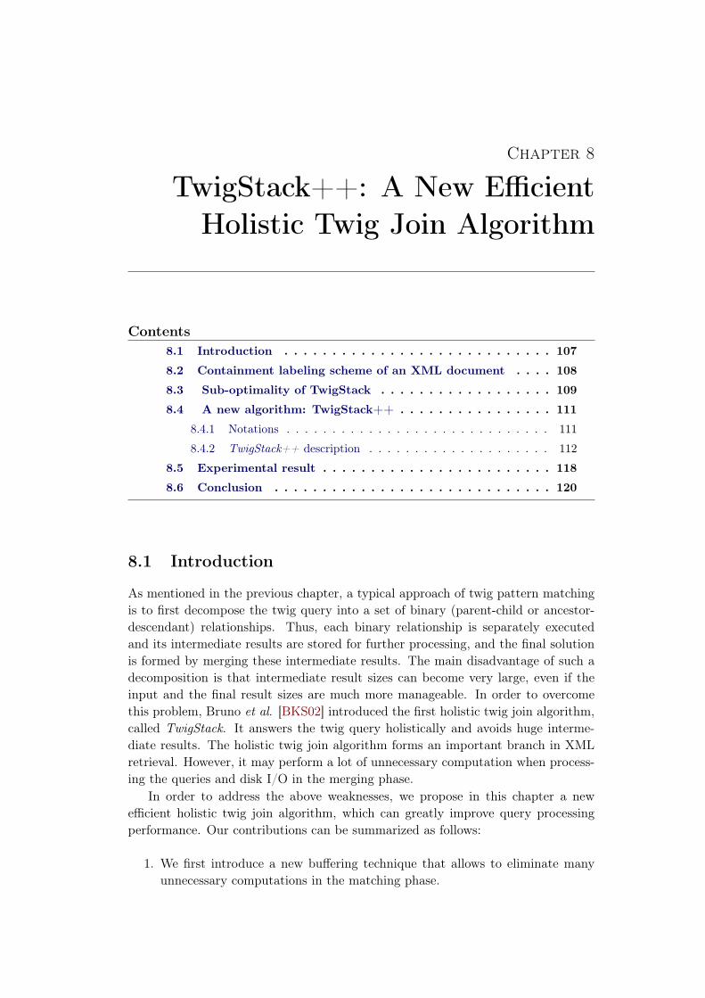
Chapter 8
TwigStack++: A New Efficient
Holistic Twig Join Algorithm
Contents
8.1 Introduction . . . . . . . . . . . . . . . . . . . . . . . . . . . . 107
8.2 Containment labeling scheme of an XML document . . . . 108
8.3 Sub-optimality of TwigStack . . . . . . . . . . . . . . . . . . 109
8.4 A new algorithm: TwigStack++ . . . . . . . . . . . . . . . . 111
8.4.1 Notations . . . . . . . . . . . . . . . . . . . . . . . . . . . . . 111
8.4.2 TwigStack++ description . . . . . . . . . . . . . . . . . . . . 112
8.5 Experimental result . . . . . . . . . . . . . . . . . . . . . . . . 118
8.6 Conclusion . . . . . . . . . . . . . . . . . . . . . . . . . . . . . 120
8.1 Introduction
As mentioned in the previous chapter, a typical approach of twig pattern matching
is to first decompose the twig query into a set of binary (parent-child or ancestor-
descendant) relationships. Thus, each binary relationship is separately executed
and its intermediate results are stored for further processing, and the final solution
is formed by merging these intermediate results. The main disadvantage of such a
decomposition is that intermediate result sizes can become very large, even if the
input and the final result sizes are much more manageable. In order to overcome
this problem, Bruno et al. [BKS02] introduced the first holistic twig join algorithm,
called TwigStack. It answers the twig query holistically and avoids huge interme-
diate results. The holistic twig join algorithm forms an important branch in XML
retrieval. However, it may perform a lot of unnecessary computation when process-
ing the queries and disk I/O in the merging phase.
In order to address the above weaknesses, we propose in this chapter a new
efficient holistic twig join algorithm, which can greatly improve query processing
performance. Our contributions can be summarized as follows:
1. We first introduce a new buffering technique that allows to eliminate many
unnecessary computations in the matching phase.
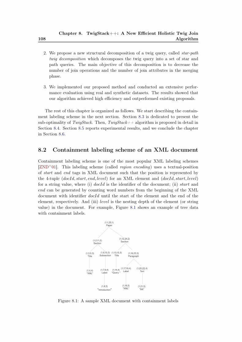
108Chapter 8. TwigStack++: A New Efficient Holistic Twig Join
Algorithm
2. We propose a new structural decomposition of a twig query, called star-pathtwig decomposition which decomposes the twig query into a set of star and
path queries. The main objective of this decomposition is to decrease the
number of join operations and the number of join attributes in the merging
phase.
3. We implemented our proposed method and conducted an extensive perfor-
mance evaluation using real and synthetic datasets. The results showed that
our algorithm achieved high efficiency and outperformed existing proposals.
The rest of this chapter is organized as follows. We start describing the contain-
ment labeling scheme in the next section. Section 8.3 is dedicated to present the
sub-optimality of TwigStack. Then, TwigStack++ algorithm is proposed in detail in
Section 8.4. Section 8.5 reports experimental results, and we conclude the chapter
in Section 8.6.
8.2 Containment labeling scheme of an XML document
Containment labeling scheme is one of the most popular XML labeling schemes
[ZND+01]. This labeling scheme (called region encoding) uses a textual-position
of start and end tags in XML document such that the position is represented by
the 4-tuple (docId, start, end, level) for an XML element and (docId, start, level)
for a string value, where (i) docId is the identifier of the document; (ii) start and
end can be generated by counting word numbers from the beginning of the XML
document with identifier docId until the start of the element and the end of the
element, respectively. And (iii) level is the nesting depth of the element (or string
value) in the document. For example, Figure 8.1 shows an example of tree data
with containment labels.
Figure 8.1: A sample XML document with containment labels
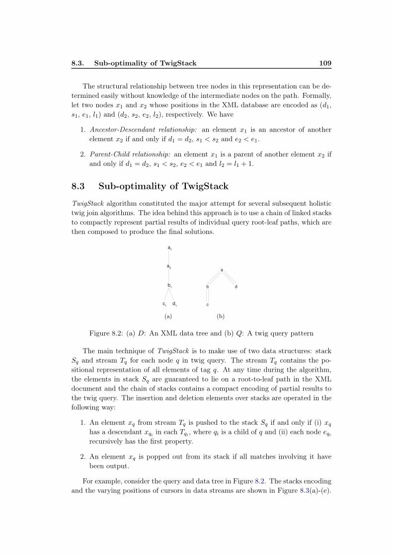
8.3. Sub-optimality of TwigStack 109
The structural relationship between tree nodes in this representation can be de-
termined easily without knowledge of the intermediate nodes on the path. Formally,
let two nodes x1 and x2 whose positions in the XML database are encoded as (d1,
s1, e1, l1) and (d2, s2, e2, l2), respectively. We have
1. Ancestor-Descendant relationship: an element x1 is an ancestor of another
element x2 if and only if d1 = d2, s1 < s2 and e2 < e1.
2. Parent-Child relationship: an element x1 is a parent of another element x2 if
and only if d1 = d2, s1 < s2, e2 < e1 and l2 = l1 + 1.
8.3 Sub-optimality of TwigStack
TwigStack algorithm constituted the major attempt for several subsequent holistic
twig join algorithms. The idea behind this approach is to use a chain of linked stacks
to compactly represent partial results of individual query root-leaf paths, which are
then composed to produce the final solutions.
(a) (b)
Figure 8.2: (a) D: An XML data tree and (b) Q: A twig query pattern
The main technique of TwigStack is to make use of two data structures: stack
Sq and stream Tq for each node q in twig query. The stream Tq contains the po-
sitional representation of all elements of tag q. At any time during the algorithm,
the elements in stack Sq are guaranteed to lie on a root-to-leaf path in the XML
document and the chain of stacks contains a compact encoding of partial results to
the twig query. The insertion and deletion elements over stacks are operated in the
following way:
1. An element xq from stream Tq is pushed to the stack Sq if and only if (i) xqhas a descendant xqi in each Tqi , where qi is a child of q and (ii) each node eqirecursively has the first property.
2. An element xq is popped out from its stack if all matches involving it have
been output.
For example, consider the query and data tree in Figure 8.2. The stacks encoding
and the varying positions of cursors in data streams are shown in Figure 8.3(a)-(e).
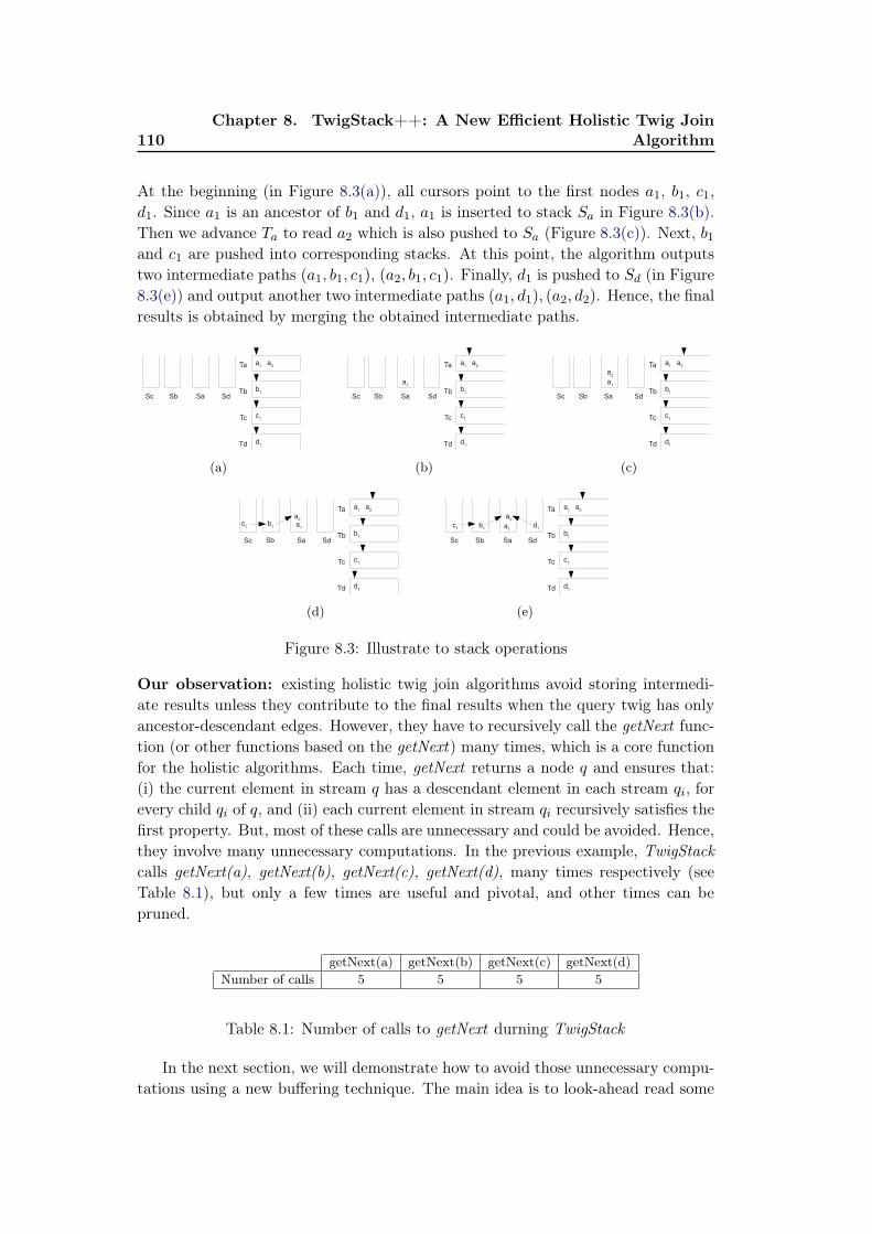
110Chapter 8. TwigStack++: A New Efficient Holistic Twig Join
Algorithm
At the beginning (in Figure 8.3(a)), all cursors point to the first nodes a1, b1, c1,
d1. Since a1 is an ancestor of b1 and d1, a1 is inserted to stack Sa in Figure 8.3(b).
Then we advance Ta to read a2 which is also pushed to Sa (Figure 8.3(c)). Next, b1and c1 are pushed into corresponding stacks. At this point, the algorithm outputs
two intermediate paths (a1, b1, c1), (a2, b1, c1). Finally, d1 is pushed to Sd (in Figure
8.3(e)) and output another two intermediate paths (a1, d1), (a2, d2). Hence, the final
results is obtained by merging the obtained intermediate paths.
(a) (b) (c)
(d) (e)
Figure 8.3: Illustrate to stack operations
Our observation: existing holistic twig join algorithms avoid storing intermedi-
ate results unless they contribute to the final results when the query twig has only
ancestor-descendant edges. However, they have to recursively call the getNext func-
tion (or other functions based on the getNext) many times, which is a core function
for the holistic algorithms. Each time, getNext returns a node q and ensures that:
(i) the current element in stream q has a descendant element in each stream qi, for
every child qi of q, and (ii) each current element in stream qi recursively satisfies the
first property. But, most of these calls are unnecessary and could be avoided. Hence,
they involve many unnecessary computations. In the previous example, TwigStackcalls getNext(a), getNext(b), getNext(c), getNext(d), many times respectively (see
Table 8.1), but only a few times are useful and pivotal, and other times can be
pruned.
getNext(a) getNext(b) getNext(c) getNext(d)
Number of calls 5 5 5 5
Table 8.1: Number of calls to getNext durning TwigStack
In the next section, we will demonstrate how to avoid those unnecessary compu-
tations using a new buffering technique. The main idea is to look-ahead read some
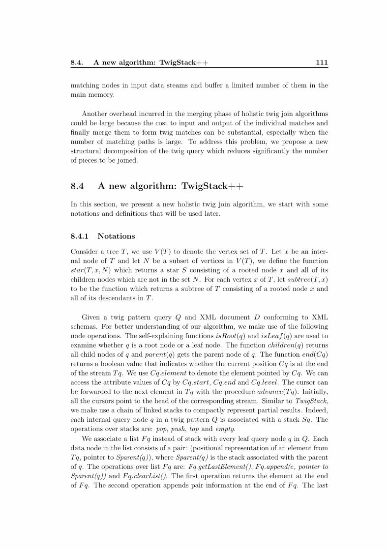
8.4. A new algorithm: TwigStack++ 111
matching nodes in input data steams and buffer a limited number of them in the
main memory.
Another overhead incurred in the merging phase of holistic twig join algorithms
could be large because the cost to input and output of the individual matches and
finally merge them to form twig matches can be substantial, especially when the
number of matching paths is large. To address this problem, we propose a new
structural decomposition of the twig query which reduces significantly the number
of pieces to be joined.
8.4 A new algorithm: TwigStack++
In this section, we present a new holistic twig join algorithm, we start with some
notations and definitions that will be used later.
8.4.1 Notations
Consider a tree T , we use V (T ) to denote the vertex set of T . Let x be an inter-
nal node of T and let N be a subset of vertices in V (T ), we define the function
star(T, x,N) which returns a star S consisting of a rooted node x and all of its
children nodes which are not in the set N . For each vertex x of T , let subtree(T, x)
to be the function which returns a subtree of T consisting of a rooted node x and
all of its descendants in T .
Given a twig pattern query Q and XML document D conforming to XML
schemas. For better understanding of our algorithm, we make use of the following
node operations. The self-explaining functions isRoot(q) and isLeaf(q) are used to
examine whether q is a root node or a leaf node. The function children(q) returns
all child nodes of q and parent(q) gets the parent node of q. The function end(Cq)
returns a boolean value that indicates whether the current position Cq is at the end
of the stream Tq. We use Cq.element to denote the element pointed by Cq. We can
access the attribute values of Cq by Cq.start, Cq.end and Cq.level. The cursor can
be forwarded to the next element in Tq with the procedure advance(Tq). Initially,
all the cursors point to the head of the corresponding stream. Similar to TwigStack,we make use a chain of linked stacks to compactly represent partial results. Indeed,
each internal query node q in a twig pattern Q is associated with a stack Sq. The
operations over stacks are: pop, push, top and empty.We associate a list Fq instead of stack with every leaf query node q in Q. Each
data node in the list consists of a pair: (positional representation of an element from
Tq, pointer to Sparent(q)), where Sparent(q) is the stack associated with the parent
of q. The operations over list Fq are: Fq.getLastElement(), Fq.append(e, pointer toSparent(q)) and Fq.clearList(). The first operation returns the element at the end
of Fq. The second operation appends pair information at the end of Fq. The last
112Chapter 8. TwigStack++: A New Efficient Holistic Twig Join
Algorithm
operation removes all elements from Fq.
The main technique of TwigStack++ is to make use of buffer Lq for each node
q in twig pattern query. For each node q, the operations over Lq are Lq.remove and
Lq.append(e). The first operation removes and returns the element at the end of Lq
and the last operation appends element e at the end of Lq.
8.4.2 TwigStack++ description
We now present our algorithm TwigStack++ for processing twig pattern matching
queries. TwigStack++ preserves the main idea of TwigStack. The objective here is
to reduce the amount of I/O and CPU cost by introducing two major improvements
as follows.
Star-path decomposition
As a first improvement, we propose a new structural decomposition of a twig query,
called star-path twig decomposition, which decomposes the twig query into a set
of star and path queries. This decomposition strategy is shown in Algorithm 1
given below, which takes as input a twig query Q. The variable SP is used to save
progressively the set of components to be generated from Q. Initially, the forest SP
is a null graph (a graph which has no vertices). For example, the structural star-pathdecomposition corresponding to the query of Figure 8.4(a) is shown in Figure 8.4(b).
Our decomposition algorithm consists of two main steps as follows: for every vertex
u of degree greater than 2:
1. path decomposition: at line 3-6 in Algorithm 1, the algorithm provides a path
for every edge (u, v) where v has degree 2. Then from Figure 8.4(a), we can
see that only one path P = (a, b, c, d) is returned for the edge (a, b).
2. star decomposition: at line 7-9, only one star is generated if and only if the
vertex u has at least one child node with degree 6= 2. Then from Figure 8.4(a),
two stars are generated for the vertices a and d.
The following theorem shows the advantage of our decomposition approach com-
pared to the root-to-leaf paths decomposition of classical holistic twig join algo-
rithms.
Theorem 8.1 The total number of join operations required for star-path twig de-composition is less than or equal to the number of join operations of the root-to-leafpaths decomposition.
Proof. In TwigStack, a (k -1)-way merge is performed in the merging phase, where
k is the number of leaf nodes in the twig query. From Algorithm 1, we can see that
for every node u of degree at least 3, we have:
8.4. A new algorithm: TwigStack++ 113
(a) (b)
Figure 8.4: (a) Tree pattern, (b) Structural star-path decomposition
Algorithm 1 Decomposition
Input: twig pattern query Q.
Output: star-path twig decomposition of Q.
1: Forest SP =null graph;
2: for every node u with degree more than 2 in Q do
3: for every child v of u with degree exactly 2 do
4: Let P = u, v, x1, · · · , xm be an induced path of Q where the nodes from x1to xm−1 has degree 2 in Q and the degree of xm is different from 2.
5: SP = SP ∪ {P}.
6: end for
7: if u has at least one child of degree 6= 2 then
8: SP = SP ∪ {star(Q, u, V (SP ))}.
9: end if
10: end for
11: return SP .
1. star-path twig decomposition approach provides a path for every edge (u, v)
where v has degree 2.
2. only one star is generated if and only if the vertex v has at least one child
node with degree 6= 2 (at line 7-9).
According to these two observations, we can see that the number of generated com-
ponents passing through the node u is less or equal to the number of children of u
which is less than or equal to the number of leaf nodes of subtree(Q, u). Therefore,
the total number of join operations of star-path twig decomposition is less than or
equal to the number of leaf nodes of any tree, giving the desired result. �
From Algorithm 1, we can easily obtain the following theorem.
Theorem 8.2 For every two different components C1 and C2 of SP , we have
|V (C1) ∩ V (C2)| ≤ 1
114Chapter 8. TwigStack++: A New Efficient Holistic Twig Join
Algorithm
Merging individual query solutions to form twig matches is simple, at least, con-
ceptually, but it may turn out to be a very expensive process in reality since the
number of join operations can be very large, rendering the merge phase cumbersome
and time consuming. By reducing the number of join operations, the performance
of XML query processing can be greatly improved. Note that our structural decom-
position will not only reduce the number of join operations but will also allow us to
decrease a large number of join attributes in the merging phase. So from Theorem
8.2, we can see that the number of join attributes is restricted to one attribute.
Improvement of getNext function
Our second improvement consists essentially in rewriting of TwigStack to elimi-
nate many unnecessary computations in the matching phase. As mentioned earlier,
TwigStack works by recursively calling a method called getNext to efficiently filter
useless elements in order to return the next node for processing. The existing holis-
tic twig join algorithms may perform many redundant checks in the calls to getNext.
We propose here a new strategy guided by containment labeling scheme to avoid
the redundant function calls. TwigStack++ changes the getNext to getNextSet func-
tion (Algorithm 2 given below). Implicitly, the getNextSet function does not return
only one node (like getNext) but a set of nodes at once. The core of this procedure
is more complex than the original algorithm but gives much better results.
In what follows, we first explain the getNextSet function and then present the
main algorithm in details. getNextSet(q) is a procedure called in the main algorithm
of TwigStack++. It updates the list Lq and returns a query node q′ (possibly q = q′)
with the following properties: at every point during computation:
1. the elements in sequence Lq (from the beginning of Lq to the end) are guar-
anteed to lie on a root-to-leaf path in the XML document.
2. for all ancestor-descendant pairs (q//q′) in the twig query, we have
∀(eq, eq′) ∈ Lq × Lq′, then eq′ is descendant of eq in XML data tree.
3. the number of buffered elements in any list is bounded by the depth of the
data tree. Note that the maximal depth of XML documents is usually very
limited.
At line 6-18 in Algorithm 2, we recursively invoke getNextSet(qi) for each qi ∈
children(q). In this computation step, we can avoid many unnecessary computa-
tions. Unlike TwigStack, it is unnecessary to recursively check whether qi and their
corresponding descendants have solution extensions if one of the following conditions
holds (this is because, the query node qi is processed already).
1. The existing top element of Sqi is decendant of the current element in the
data stream of node q.
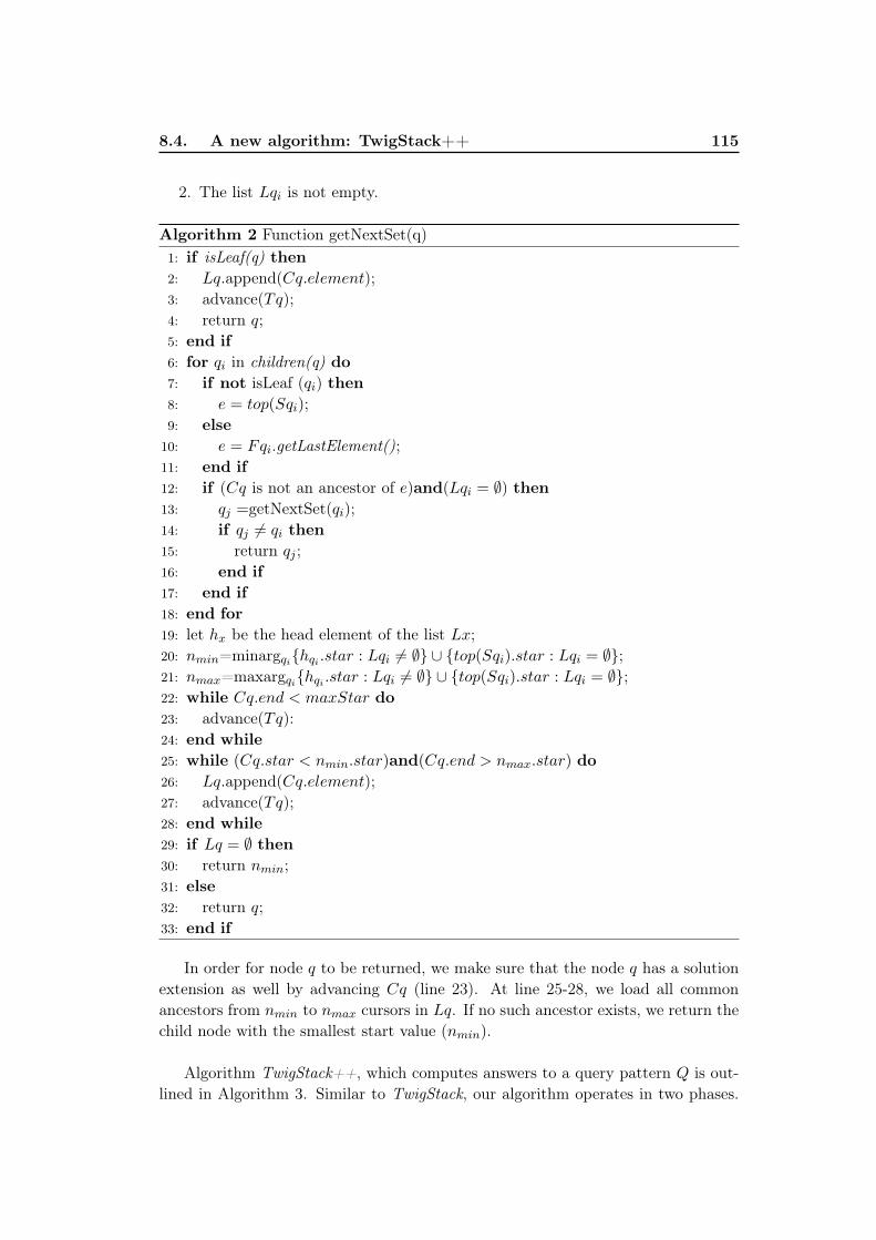
8.4. A new algorithm: TwigStack++ 115
2. The list Lqi is not empty.
Algorithm 2 Function getNextSet(q)
1: if isLeaf(q) then
2: Lq.append(Cq.element);
3: advance(Tq);
4: return q;
5: end if
6: for qi in children(q) do
7: if not isLeaf (qi) then
8: e = top(Sqi);
9: else
10: e = Fqi.getLastElement();11: end if
12: if (Cq is not an ancestor of e)and(Lqi = ∅) then
13: qj =getNextSet(qi);
14: if qj 6= qi then
15: return qj ;
16: end if
17: end if
18: end for
19: let hx be the head element of the list Lx;
20: nmin=minargqi{hqi .star : Lqi 6= ∅} ∪ {top(Sqi).star : Lqi = ∅};
21: nmax=maxargqi{hqi .star : Lqi 6= ∅} ∪ {top(Sqi).star : Lqi = ∅};
22: while Cq.end < maxStar do
23: advance(Tq):
24: end while
25: while (Cq.star < nmin.star)and(Cq.end > nmax.star) do
26: Lq.append(Cq.element);
27: advance(Tq);
28: end while
29: if Lq = ∅ then
30: return nmin;
31: else
32: return q;
33: end if
In order for node q to be returned, we make sure that the node q has a solution
extension as well by advancing Cq (line 23). At line 25-28, we load all common
ancestors from nmin to nmax cursors in Lq. If no such ancestor exists, we return the
child node with the smallest start value (nmin).
Algorithm TwigStack++, which computes answers to a query pattern Q is out-
lined in Algorithm 3. Similar to TwigStack, our algorithm operates in two phases.
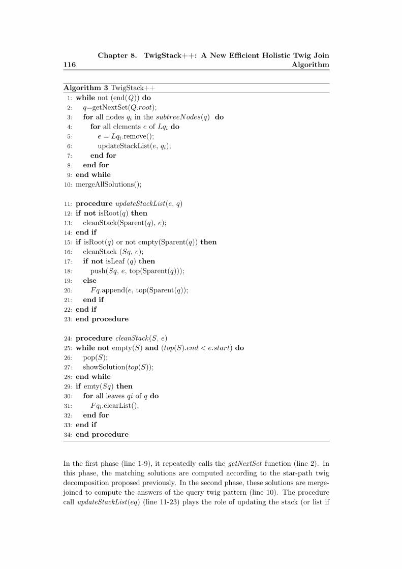
116Chapter 8. TwigStack++: A New Efficient Holistic Twig Join
Algorithm
Algorithm 3 TwigStack++
1: while not (end(Q)) do
2: q=getNextSet(Q.root);
3: for all nodes qi in the subtreeNodes(q) do
4: for all elements e of Lqi do
5: e = Lqi.remove();
6: updateStackList(e, qi);
7: end for
8: end for
9: end while
10: mergeAllSolutions();
11: procedure updateStackList(e, q)12: if not isRoot(q) then
13: cleanStack(Sparent(q), e);
14: end if
15: if isRoot(q) or not empty(Sparent(q)) then
16: cleanStack (Sq, e);
17: if not isLeaf (q) then
18: push(Sq, e, top(Sparent(q)));
19: else
20: Fq.append(e, top(Sparent(q));
21: end if
22: end if
23: end procedure
24: procedure cleanStack(S, e)
25: while not empty(S) and (top(S).end < e.start) do
26: pop(S);
27: showSolution(top(S));
28: end while
29: if emty(Sq) then
30: for all leaves qi of q do
31: Fqi.clearList();
32: end for
33: end if
34: end procedure
In the first phase (line 1-9), it repeatedly calls the getNextSet function (line 2). In
this phase, the matching solutions are computed according to the star-path twig
decomposition proposed previously. In the second phase, these solutions are merge-
joined to compute the answers of the query twig pattern (line 10). The procedure
call updateStackList(eq) (line 11-23) plays the role of updating the stack (or list if
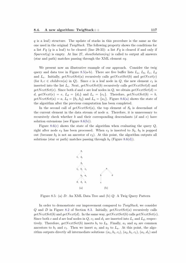
8.4. A new algorithm: TwigStack++ 117
q is a leaf) structure. The update of stacks in this procedure is the same as the
one used in the original TwigStack. The following property shows the conditions for
a list Fq (q is a leaf) to be cleared (line 29-33): a list Fq is cleared if and only if
Sparent(q) is empty. At line 27, showSolution(eq) is called to output all answers
(star and path) matches passing through the XML element eq.
We present now an illustrative example of our approach. Consider the twig
query and data tree in Figure 8.5(a-b). There are five buffer lists La, Lb, Lc, Ld
and Le. Initially, getNextSet(a) recursively calls getNextSet(b) and getNext(c)
(for b, c ∈ children(a) in Q). Since c is a leaf node in Q, the new element c1 is
inserted into the list Lc. Next, getNextSet(b) recursively calls getNextSet(d) and
getNextSet(e). Since both d and e are leaf nodes in Q, we obtain getNextSet(d) =
d, getNext(e) = e, Ld = {d1} and Le = {e1}. Therefore, getNextSet(b) = b,
getNextSet(a) = a, Lb = {b1, b2} and La = {a1}. Figure 8.6(a) shows the state of
the algorithm after the previous computation has been completed.
In the second call of getNextSet(a), the top element of Sb is descendant of
the current element in the data stream of node a. Therefore, it is unnecessary to
recursively check whether b and their corresponding descendants (d and e) have
solution extensions (see Figure 8.6(b)).
Figure 8.6(c) shows the state of the algorithm when evaluating the query Q,
right after node e2 has been processed. When e2 is inserted to S2, b2 is popped
out (because b2 is not an ancestor of e2). At this point, the algorithm outputs all
solutions (star or path) matches passing through b2 (Figure 8.6(d)).
(a) (b)
Figure 8.5: (a) D: An XML Data Tree and (b) Q: A Twig Query Pattern
In order to demonstrate our improvement compared to TwigStack, we consider
Q and D in Figure 8.2 of Section 8.3. Initially, getNextSet(a) recursively calls
getNextSet(b) and getNext(d). In the same way, getNextSet(b) calls getNextSet(c).
Since both c and d are leaf nodes in Q, c1 and d1 are inserted into Lc and Ld, respec-
tively. Therefore, getNextSet(b) inserts b1 to Lb. Finally, a1 and a2 are common
ancestors to b1 and c1. Then we insert a1 and a2 to La. At this point, the algo-
rithm outputs directly all intermediate solutions :(a1, b1, c1), (a2, b1, c1), (a1, d1) and
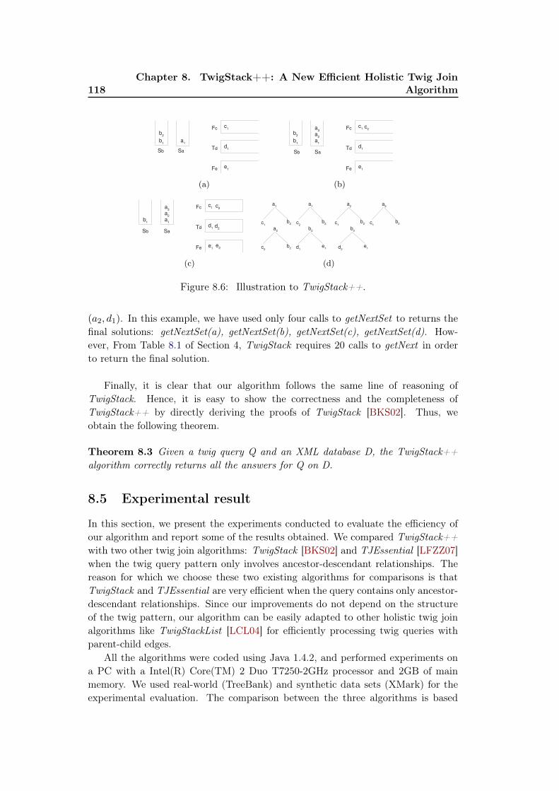
118Chapter 8. TwigStack++: A New Efficient Holistic Twig Join
Algorithm
(a) (b)
(c) (d)
Figure 8.6: Illustration to TwigStack++.
(a2, d1). In this example, we have used only four calls to getNextSet to returns the
final solutions: getNextSet(a), getNextSet(b), getNextSet(c), getNextSet(d). How-
ever, From Table 8.1 of Section 4, TwigStack requires 20 calls to getNext in order
to return the final solution.
Finally, it is clear that our algorithm follows the same line of reasoning of
TwigStack. Hence, it is easy to show the correctness and the completeness of
TwigStack++ by directly deriving the proofs of TwigStack [BKS02]. Thus, we
obtain the following theorem.
Theorem 8.3 Given a twig query Q and an XML database D, the TwigStack++algorithm correctly returns all the answers for Q on D.
8.5 Experimental result
In this section, we present the experiments conducted to evaluate the efficiency of
our algorithm and report some of the results obtained. We compared TwigStack++with two other twig join algorithms: TwigStack [BKS02] and TJEssential [LFZZ07]
when the twig query pattern only involves ancestor-descendant relationships. The
reason for which we choose these two existing algorithms for comparisons is that
TwigStack and TJEssential are very efficient when the query contains only ancestor-
descendant relationships. Since our improvements do not depend on the structure
of the twig pattern, our algorithm can be easily adapted to other holistic twig join
algorithms like TwigStackList [LCL04] for efficiently processing twig queries with
parent-child edges.
All the algorithms were coded using Java 1.4.2, and performed experiments on
a PC with a Intel(R) Core(TM) 2 Duo T7250-2GHz processor and 2GB of main
memory. We used real-world (TreeBank) and synthetic data sets (XMark) for the
experimental evaluation. The comparison between the three algorithms is based
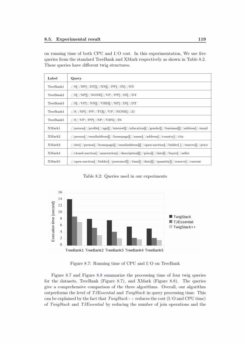
8.5. Experimental result 119
on running time of both CPU and I/O cost. In this experimentation, We use five
queries from the standard TreeBank and XMark respectively as shown in Table 8.2.
These queries have different twig structures.
Label Query
TreeBank1 //S[//NP[//DT][//NN]]//PP[//IN]//NN
TreeBank2 //S[//NP][//NONE]//VP//PP[//IN]//DT
TreeBank3 //S[//VP[//NN][//VBD]]//NP[//IN]//DT
TreeBank4 //S//NP[//PP//TO][//VP//NONE]//JJ
TreeBank5 //S//VP//PP[//NP//VBN]//IN
XMark1 //person[//profile[//age][//interest][//education][//gender][//business]][//address]//email
XMark2 //person[//emailaddress][//homepage][//name]//address[//country]//city
XMark3 //site[//person[//homepage][//emailaddress]][//open-auction[//bidder] [//reserve]]//price
XMark4 //closed-auction[//annotation[//description]][//price][//date][//buyer]//seller
XMark5 //open-auction[//bidder[//personref][//time][//date]][//quantity][//reserve]//current
Table 8.2: Queries used in our experiments
Figure 8.7: Running time of CPU and I/O on TreeBank
Figure 8.7 and Figure 8.8 summarize the processing time of four twig queries
for the datasets, TreeBank (Figure 8.7), and XMark (Figure 8.8). The queries
give a comprehensive comparison of the three algorithms. Overall, our algorithm
outperforms the level of TJEssential and TwigStack in query processing time. This
can be explained by the fact that TwigStack++ reduces the cost (I/O and CPU time)
of TwigStack and TJEssential by reducing the number of join operations and the

120Chapter 8. TwigStack++: A New Efficient Holistic Twig Join
Algorithm
Figure 8.8: Running time of CPU and I/O on XMark
number of join attributes in the merging phase and the unnecessary computations
in the matching phase.
8.6 Conclusion
In this chapter, we have proposed a new holistic twig join algorithm, called TwigStack++to efficiently process XML twig patterns. Our approach is based on two main im-
provements in the matching and merging phase. Experimental results show that
our approach achieves high efficiency and outperforms existing proposals.
Chapter 9
Conclusion and Future Work
In this thesis, we discussed three graph theory problems applied to different classes
of labeled graphs. In this chapter, we present several open questions and directions
for future research in these areas.
******
Over the years, several vertex-distinguishing edge coloring variants have been de-
fined in the literature. We gave in Chapter three a survey of various methods,
recent results and open conjectures from this area of research. In particular, we
have detailed the vertex-distinguishing edge coloring problem by sets and multisets.
Originally motivated by these two variants, we investigated in Chapter four a new
variant of edge coloring that induces a vertex distinguishing labeling where the label
of each vertex is given by the difference between the highest and the lowest colors
of its adjacent edges. In view of our results, we observed that our parameter can
be used to get a bound on the detection number. In addition, several results have
been obtained for various classes of graphs.
As future works, we plan to focus on the following three issues.
1. We left as an open question to show that the gap chromatic number of a graph
of order n is always in {n− 1, n, n+ 1}.
2. The computational complexity of the gap chromatic number is still an open
problem (this is the case of most variants of vertex distinguishing problems
derived from an improper edge coloring).
3. As for the other distinguishing parameters, it would be interesting to consider
the variant of the gap coloring problem that distinguishes adjacent vertices
only.
******
The purpose of the second part of this thesis was to study the graph packing problem
for labeled graphs. Much work has been done on the unlabeled graph packing prob-
lem and we felt that investigating the labeled case might yield interesting results.
The first section of Chapter five was dedicated to giving the reader an introduc-
tion to some relevant results on the packing of unlabeled graphs. Then, we studied
122 Chapter 9. Conclusion and Future Work
the labeled graph packing problems for k copies of cycles in which we have proved
the exact value of λk(G) for all n ≥ 4k − 3. In Chapter six, we computed upper
bounds for the labeled embedding number of trees and (n, n−2)-graphs. From these
results, we can consider several directions for future work:
1. We would like to prove Conjecture 5.28 (in Chapter 5) that deals with the
labeled packing of k copies of cycles of order n, where 2k + 1 ≤ n ≤ 4k − 3.
2. we hope that the work in Chapter 6 provides a helpful beginning to the study
of the labeled packing of three copies of trees and (n, n− 2)-graphs.
3. Characterize all trees T for which the labeled embedding number of T reaches
the upper bound of Lemma 5.21.
4. We would also like to improve the lower bound of the labeled embedding
number of (n, n − 2)-graphs from ⌊2n3 ⌋ to ⌊3n4 ⌋ − 2 (as shown in Conjecture
6.15).
******
The last part of this thesis addresses the problem of query processing in XML
databases, namely XML twig queries. An XML twig query, represented as a la-
beled tree, is essentially a complex selection on the structure of an XML document.
Thus, XML tree patten matching is widely regarded as a new challenge for efficient
XML query processing. Until now, the holistic twig join approach was regarded
as the most efficient family in the literature. In Chapter seven, we provided a
comprehensive survey of the basic ideas and results of the main holistic twig join
algorithms available in the literature. In Chapter eight, we proposed a novel
holistic twig join algorithm, called TwigStack++. This algorithm is based on two
main improvements in the decomposition and matching phases. We analytically
and experimentally shown that TwigStack++ can efficiently avoid many unneces-
sary computation and I/O cost. While this part has proposed an efficient algorithm
for XML tree pattern matching, a number of issues need to be further investigated.
1. We would like to combine our decomposition technique with other efficient
holistic twig join algorithms. Furthermore it would also be interesting to
study the parallelism of these algorithms on a multi-core system in order to
maximize the computing performance of query processing in a large XML
database.
2. In the literature, quantum algorithms have attracted considerable attention
in the theoretical computer science community because of the considerable
speed up over classical algorithms they achieve. For a practical perspective
of tree matching problem, several aspects remains to be investigated. Indeed,
quantum versions of matching approaches based on decomposition and com-
binatorics on words can be developed. Nevertheless, the formalization of such
123
solutions may be very difficult, but very promising. One can address that in
the future.
3. As mentioned in Part two, the graph matching problem can be naturally
stated as a packing of labeled graphs. Therefore, it would be interesting to
exploit tree packing techniques in order to define a coherent similarity measure
between XML query and tree data.

Bibliography
[AADR05] L. Addario-Berry, R. E. L. Aldred, K. Dalal, and B. A. Reed. Vertex
colouring edge partitions. J. Combin. Theory (B), 94:237–244, 2005.
(Cited on page 18.)
[AB93] M. Aigner and S. Brandt. Embedding arbitrary graphs of maximum
degree two. J. London Math. Soc, 48:39–51, 1993. (Cited on page 50.)
[AC75] A. V. Aho and M. J. Corasick. Efficient string matching: An aid to
bibliographic search. Commun. ACM, pages 333–340, 1975. (Cited on
page 97.)
[AC96] M. Albertson and K. Collins. Symmetry breaking in graphs. ElectronicJournal of Combinatorics, 3:43–55, 1996. (Cited on page 16.)
[AF96] N. Alon and E. Fischer. 2-factors in dense graphs. Discrete Math, 152:1–
3, 1996. (Cited on page 50.)
[AJK+02] S. Al-Khalifa, H. V. Jagadish, N. Koudas, J. M. Patel, D. Srivastava,
and Y. Wu. Structural joins: a primitive for efficient XML query pattern
matching. In Proceedings of the 18th International Conference on DataEngineering, San Jose: IEEE, pages 141–152, 2002. (Cited on pages 99
and 105.)
[ATT92] M. Aigner, E. Triesch, and Z. Tuza. Irregular assignments and vertex-
distinguishing edge colorings of graphs. Combinatorics ’90, Proc. Conf.,Gaeta/Italy 1990, Elsevier Science Pub., New York, pages 1–9, 1992.
(Cited on pages 17, 18 and 20.)
[AYL06] S. Amer-Yahia and M. Lalmas. XML search: languages, INEX and
scoring. ACM SIGMOD Rec., 35(4):16–23, 2006. (Cited on page 95.)
[BBLW99] C. Bazgan, A. H. Benhamdine, H. Li, and M. Wozniak. On the vertex-
distinguishing proper edge-colorings of graphs. J. Combin. Theory Ser.B, 75(2):288–301, 1999. (Cited on page 18.)
[BBLW01] C. Bazgan, A. H. Benhamdine, H. Li, and M. Wozniak. A note on
the vertex-distinguishing proper coloring of graphs with large minimum
degree. Discrete Math, 236:37–42, 2001. (Cited on page 19.)
[BBS02] P. N. Balister, B. Bollobas, and R. H Schelp. Vertex distinguishing
colorings of graphs with △(g) = 2. Discrete Math, 252:17–29, 2002.
(Cited on page 18.)
126 Bibliography
[BE78] B. Bollobás and S.E. Eldridge. Packing of graphs and applications to
computational complexity. J. Comb. Theory Ser, B, 25:105–124, 1978.
(Cited on pages 46, 47 and 49.)
[Beh65] M. Behzad. Graphs and their chromatic numbers. Ph.D. Thesis, Michi-gan State University, 1965. (Cited on page 16.)
[Ber60] C. Berge. Les problèmes de coloration en théorie des graphes. Publicationde l’Institut de Statistique de l’Université de Paris 9, pages 123–160,
1960. (Cited on page 15.)
[Ber61] C. Berge. Färbung von graphen, deren sämtliche bzw, deren ungerade
kreise starr sind. In Wissenschaftliche Zeitschrift. Martin Luther Uni-versitat Halle Wittenberg 10, pages 114–115, 1961. (Cited on page 15.)
[BKN08] B. Bollobás, A. Kostochka, and K. Nakprasit. Packing d-degenerate
graphs. J. Comb. Theory, Ser. B, 98(1):85–94, 2008. (Cited on page 50.)
[BKS02] N. Bruno, N. Koudas, and D. Srivastava. Holistic twig joins: optimal
XML pattern matching. In Proceedings of the 2002 ACM SIGMOD inter-national conference on Management of data, Madison, Wisconsin, USA,
SIGMOD ’02, pages 310–321, New York, NY, USA, 2002. ACM. (Cited
on pages 99, 105, 107 and 118.)
[BKT05] L. Baril, H. Kheddouci, and O. Togni. The irregularity strength of cir-
culant graphs. Discrete Math, 304(1-3):1–10, 2005. (Cited on page 17.)
[Bol78] B. Bollobás. Extremal Graph Theory. Academic Press, London, 1978.
(Cited on pages 46 and 47.)
[Bro41] R. L. Brooks. On colouring the nodes of a network. Proc. CambridgePhilos. Soc, 37:194–197, 1941. (Cited on page 14.)
[BS77] D. Burns and S. Schuster. Every (p, p − 2)-graph is contained in its
complement. J. Graph Theory, pages 277–f279, 1977. (Cited on page 47.)
[BS78] D. Burns and S. Schuster. Embedding (n, n− 1)-graphs in their comple-
ments. Israel J. Math, 30:313–320, 1978. (Cited on pages 48 and 49.)
[BS97] A. C. Burris and R. H. Schelp. Vertex-distinguishing proper edge color-
ings. J. Graph Theory, 26:73–82, 1997. (Cited on pages 17 and 18.)
[Bur88] J. Burghardt. A tree pattern matching algorithm with reasonable space
requirements. In CAAP’88, pages 1–15, 1988. (Cited on page 97.)
[Bur93] A. C. Burris. Vertex-distinguishing edge-colorings. Ph.D. Dissertation,Memphis State University, 1993. (Cited on page 17.)
[Bur94] A. C. Burris. On graphs with irregular coloring number 2. Congr. Nu-merantium, 100:129–140, 1994. (Cited on page 20.)
Bibliography 127
[Bur95] A. C. Burris. The irregular coloring number of a tree. Discrete Math,
141:279–283, 1995. (Cited on pages 17, 20 and 50.)
[BW85] A. Benhocine and A.P. Wojda. On self-complementation. J. GraphTheory, 8:85–91, 1985. (Cited on page 51.)
[BW04] S. Brandt and M. Wozniak. On cyclic packing of a tree. Graphs andCombinatorics, 20(4):435–442, 2004. (Cited on page 49.)
[Cat74] P. A. Catlin. Subgraphs of graphs. Discrete Math, 10:225–233, 1974.
(Cited on page 46.)
[CDG+09] A. Campi, E. Damiani, S. Guinea, S. Marrara, G. Pasi, and P. Spoletini.
A fuzzy extension of the XPath query language. Journal of IntelligentInformation Systems, 33(3):285–305, 2009. (Cited on page 95.)
[CEOZ06] G. Chartrand, H. Escuadro, F. Okamota, and P. Zhang. Detectable
colorings of graphs. Utilitas Mathematica, 69:13–32, 2006. (Cited on
pages 17 and 20.)
[CH90] F. C. Chow and J. L. Hennessy. The priority-based coloring approach
to register allocation. Proc. Cambridge Philos. Soc, 12(4):501–536, 1990.
(Cited on page 14.)
[CH97] R. Cole and R. Hariharan. Tree pattern matching and subset matching
in randomized o(nlog3m) time. In Proceedings of the twenty-ninth annualACM symposium on Theory of computing, pages 66–75, New York, NY,
USA, 1997. ACM. (Cited on pages 97 and 98.)
[CH03] R. Cole and R. Hariharan. Tree pattern matching to subset matching
in linear time. In SIAM J. Computing, 32:1056–1066, 2003. (Cited on
pages 97 and 98.)
[Cha87] D. R. Chase. An improvement to bottom-up tree pattern matching. In
POPL’87, pages 168–177, 1987. (Cited on page 97.)
[CHS96] J. Cerny, M. Hornak, and R. Sotak. Observability of a graph. Math.Slovaca, 46:21–31, 1996. (Cited on pages 17 and 18.)
[CJL+88] G. Chartrand, M. S. Jacobson, J. Lehel, O. R. Oellermann, S. Ruiz, and
F. Saba. Irregular networks. Congr. Numerantium, 64:187–192, 1988.
(Cited on pages 17 and 18.)
[CLL05] T. Chen, J. Lu, and T. W. Ling. On boosting holism in XML twig
pattern matching using structural indexing techniques. In SIGMOD 05,
pages 455–466, 2005. (Cited on pages 100 and 105.)
128 Bibliography
[CLT+06] S. Chen, H. G. Li, J. Tatemura, W. P. Hsiung, D. Agrawal, and K. S.
Candan. Twig2Stack: bottom-up processing of generalized-tree-pattern
queries over XML documents. In Proceedings of the 32nd internationalconference on Very large data bases, VLDB ’06, pages 283–294, 2006.
(Cited on pages 101 and 105.)
[CSS03] B. Csaba, A. Shokoufandeh, and E. Szemerédi. Proof of a conjecture of
bollobás and eldridge for graphs of maximum degree three. Combinator-ica, 23:35–72, 2003. (Cited on page 50.)
[CZ05] G. Chartrand and P. Zhang. Introduction to graph theory. McGraw-Hill,
New York, 2005. (Cited on page 5.)
[CZ08] G. Chartrand and P. Zhang. Chromatic Graph Theory. Chapman and
Hall/CRC. Press, Boca Raton, 2008. (Cited on page 17.)
[DC08] D.B. Dao and J. Cao. A glance on current XML twig pattern matching
algorithms. In ICCSA (2)’08, pages 307–321, 2008. (Cited on page 102.)
[DGM94] M. Dubiner, Z. Galil, and E. Magen. Faster tree pattern matching. J.ACM, 41:205–213, 1994. (Cited on page 97.)
[Eat00] N. Eaton. A near packing of two graphs. J. Comb. Theory Ser. B,
80:98–103, 2000. (Cited on page 50.)
[EG59] P. Erdős and T. Gallai. On maximal paths and circuits of graphs. ActaMath. Acad. Sci. Hungar, 10:337–356, 1959. (Cited on page 47.)
[EG74] R. C. Entringer and L. D. Gassman. Line-critical point determining
and point distinguishing graphs. Discrete Mathematics, 10:43–55, 1974.
(Cited on page 16.)
[EP05] H. Escuadro and Z. Ping. On detectable colorings of graphs. MathematicaBohemica, 130:427–445, 2005. (Cited on page 20.)
[Eul41] L. Euler. Solutio problematis ad geometriam situs pertinentis. AcademiaeSci. I. Petropolitanae, 8:128–140, 1741. (Cited on page 1.)
[FMP+12] E. Flandrin, A. Marczyk, J. Przybylo, J. F. Sacló, and M. Wozniak.
Neighbor sum distinguishing index. Graphs and Combinatorics, pages
1–8, 2012. (Cited on page 18.)
[FRSS81] R. J. Faudree, C.C. Rousseau, R.H. Schelp, and S. Schuster. Embedding
graphs in their complements. Czechoslovak Math. J, 31(106):53–62, 1981.
(Cited on pages 49, 50 and 51.)
[Gam86] A. Gamst. Some lower bounds for a class of frequency assignment prob-
lems. IEEE Transactions on Vehicular Technology, 35(1):8–14, 1986.
(Cited on page 14.)
Bibliography 129
[GHPW08] E. Györi, M. Hornák, C. Palmer, and M. Wozniak. General neighbour-
distinguishing index of a graph. Discrete Mathematics, pages 827–831,
2008. (Cited on page 18.)
[GJ79] M. Garey and D. Johnson. Computers and Intractability: A Guide to theTheory of NP-Completeness. W.H. Freman and Company, New York,
1979. (Cited on page 14.)
[GLS84] M. Grötschel, L. Lovàsz, and A. Schrijver. Polynomial algorithms for
perfect graphs. Annals of Discrete Mathematic, 21:169–197, 1984. (Cited
on page 15.)
[GZ09] G. Görlich and A. Zak. A note on packing graphs without cycles of length
up to five. Electr. J. Comb, 16(1), 2009. (Cited on page 50.)
[Haj91] P. Hajnal. An ω(n43 ) lower bound on the randomized decision tree com-
plexity of graph properties. Combinatorica, 11:131–143, 1991. (Cited on
page 47.)
[Har69] F. Harary. Graph Theory. Addison-Wesley Publishing Company, Read-
ing, Massachusetts, 1969. (Cited on page 5.)
[Har96] F. Harary. Survey of methods of automorphism destruction in
graphs. Invited address, Eighth Quadrennial International Conferenceon Graph Theory, Combinatorics, Algorithms and Applications, Kala-mazoo, Michigan, 1996. (Cited on page 16.)
[Har01] F. Harary. Methods of destroying the symmetries of a graph. Bull.Malaysian Math. Sci. Soc, 24(2):183–191, 2001. (Cited on page 16.)
[HHS81] S.M. Hedetuiemi, S.T. Hedetniemi, and P.J. Slater. A note on packing
two trees into kn. Ars Combin, 11:149–153, 1981. (Cited on page 48.)
[HK86] S. L. Hakimi and O. Kaziv. On a generalization of edge-coloring in
graphs. Journal of Graph Theory, pages 139–154, 1986. (Cited on
page 16.)
[HL09] S. C. Haw and C. S. Lee. Node labeling schemes in XML query opti-
mization: A survey and trends. IETE Technical Review, 26(2):88–100,
2009. (Cited on page 103.)
[HM76] F. Harary and R. A. Melter. On the metric dimension of a graph. ArsCombin, 2:191–195, 1976. (Cited on page 16.)
[HO82] C. M. Hoffman and M. J. O’Donnell. Pattern matching in trees. J. ACM,
pages 68–95, 1982. (Cited on pages 96 and 97.)
[Hol81] I. Holyer. The np-completeness of edge-colouring. SIAM J. Comput,10(4):718–720, 1981. (Cited on page 15.)
130 Bibliography
[HP85] F. Harary and M. Plantholt. The point-distinguishing chromatic index.
Graphs and Applications. Wiley, New York, pages 147–162, 1985. (Cited
on pages 17, 18, 20 and 21.)
[HR78] C. Huang and A. Rosa. Decomposition of complete graphs into trees.
Ars Combin, 5:26–63, 1978. (Cited on page 49.)
[HS70] A. Hajnal and E. Szemerédi. Proof of conjecture of erdos. in: Combi-natorial Theory and its Applications (P. Erdos, A. Renyi and V. T. SosEditors), North-Holland, pages 601–623, 1970. (Cited on page 50.)
[HS97] M. Hornak and R. Sotak. Localization of jumps of the point-
distinguishing chromatic index of kn,m. Discuss. Math. Graph Theory,17:243–251, 1997. (Cited on page 20.)
[HS06] M. Hornak and N. Zagaglia Salvi. On the point-distinguishing chromatic
index of complete bipartite graphs. Ars Combinatoria, 80:75–85, 2006.
(Cited on page 20.)
[HW82] A. J. W. Hilton and D. de Werra. Sufficient conditions for balanced and
for equitable edge-colorings of graphs. O. R. Working paper 82/3, Déptof Math., École Polytechnique Fédérate de Lansanne, Switzerland, 1982.
(Cited on page 16.)
[IHH09] S. K. Izadi, T. Harder, and M. S. Haghjoo. S3: Evaluation of tree-pattern
XML queries supported by structural summaries. In Proceedings of Dataand Knowledge Engineering, pages 126–145, 2009. (Cited on pages 103,
104 and 105.)
[JLH+07] Z. Jiang, C. Luo, W. C. Hou, Q. Zhu, and D. Che. Efficient processing
of XML twig pattern: A novel one-phase holistic solution. In DEXA 07,
pages 87–97, 2007. (Cited on pages 101 and 105.)
[JWLY03] H. Jiang, W. Wang, H. Lu, and J. X. Yu. Holistic twig joins on indexed
XML documents. In Proceedings of VLDB, pages 273–284, 2003. (Cited
on pages 101 and 105.)
[JY12] Z. Jun-qiao and B. Yue-hua. Upper bounds on vertex distinguishing
chromatic index of some halin graphs. Discrete Mathematics, 27(3):329–
334, 2012. (Cited on page 19.)
[Kaz12] J. S. Kaziów. Multiplicative vertex-colouring weightings of graphs. In-formation Processing Letters, 112:191–194, 2012. (Cited on pages 17
and 18.)
[Khe03] H. Kheddouci. A note on packing of two copies of some trees into their
third power. Applied Mathematics Letters, 16:1115–1121, 2003. (Cited
on page 52.)
Bibliography 131
[KKY08] H. Kaul, A. Kostochka, and G. Yu. On a graph packing conjecture by
bollobás, eldridge and catlin. Combinatorica, 28(4):469–485, 2008. (Cited
on page 50.)
[KLT04] M. Karoóski, T. Luczak, and A. Thomason. Edge weights and vertex
colours. J. Combin. Theory Ser. B, 91(1):151–157, 2004. (Cited on
page 18.)
[KMSW01] H. Kheddouci, S. Marshall, J. F. Saclé, and M. Wozniak. On the packing
of three graphs. Discrete Mathematics, 236((1-3)):197–225, 2001. (Cited
on page 47.)
[Kos89] S. R. Kosaraju. Efficient tree pattern matching. In Proceedings of the 30thAnnual Symposium on Foundations of Computer Science, pages 178–
183, Washington, DC, USA, 1989. IEEE Computer Society. (Cited on
page 97.)
[L7́2] L. László. Normal hypergraphs and the perfect graph conjecture. DiscreteMathematics, 2(3):253–267, 1972. (Cited on page 15.)
[LB09] M. Lalmas and R. Baeza-Yates. Structured document retrieval. In En-cyclopedia of Database Systems, pages 2867–2868. Springer, 2009. (Cited
on page 94.)
[LCL04] J. Lu, T. Chen, and T. W. Ling. Efficient processing of XML twig pat-
terns with parent child edges: a look-ahead approach. In Proceedings ofthe 13th ACM international Conference on Information and KnowledgeManagement (CIKM), Washington D.C., USA, pages 533–542, 2004.
(Cited on pages 100, 105 and 118.)
[Lei79] F. T. Leighton. A graph coloring algorithm for large sceduling problems.
Journal of Research of the National Bureau of Standards, 84(6):489–503,
1979. (Cited on page 14.)
[LFZZ07] G. Li, J. Feng, Y. Zhang, and L. Zhou. Efficient holistic twig joins
in leaf-to-root combining with root-to-leaf way. In DASFAA, Bangkok,Thailand, pages 834–849, 2007. (Cited on pages 101, 105 and 118.)
[LLCC05] J. Lu, T. W. Ling, C. Y. Chan, and T. Chen. From region encoding to
extended Dewey: On efficient processing of XML twig pattern matching.
In Proceedings of the 31st International Conference on Very Large DataBases (VLDB), Trondheim, Norway, pages 193–204, 2005. (Cited on
pages 101, 102 and 105.)
[LML11] J. Lu, X. Meng, and T. W. Ling. Indexing and querying XML using
extended dewey labeling scheme. Data Knowl. Eng., 70:35–59, 2011.
(Cited on pages 102 and 105.)
132 Bibliography
[Luc92] D. E. Lucas. Récréations mathématiques. Gauthiers Villars, Paris, 2,
1892. (Cited on page 55.)
[LW08a] J. Li and J. Wang. Fast matching of twig patterns. In Proceedings of the19th international conference on Database and Expert Systems Applica-tions, DEXA ’08, pages 523–536, 2008. (Cited on pages 101 and 105.)
[LW08b] J. Li and J. Wang. Twigbuffer: avoiding useless intermediate solutions
completely in twig joins. In Proceedings of the 13th international confer-ence on Database systems for advanced applications, DASFAA’08, pages
554–561, 2008. (Cited on pages 100 and 105.)
[NNS88] S. Nakano, T. Nishizeki, and N. Saito. On the f -coloring of multigraphs.
IEEE Trans. Circuit and Syst, 35(3):345–353, 1988. (Cited on page 16.)
[QYD07] Lu Qin, Jeffrey Xu Yu, and Bolin Ding. Twiglist: make twig pattern
matching fast. In Proceedings of the 12th international conference onDatabase systems for advanced applications (DASFAA), DASFAA’07,
pages 850–862, Berlin, Heidelberg, 2007. (Cited on pages 101 and 105.)
[RM04] P. Rao and B. Moon. Prix: Indexing and querying XML using prüfer se-
quences. In ICDE’04, pages 288–300, 2004. (Cited on pages 103 and 105.)
[RS08] J. Rudasov and R. Sotak. Vertex-distinguishing proper edge colourings
of some regular graphs. Discrete Mathematics, 308(5-6):795–802, 2008.
(Cited on page 18.)
[SA89] A. Sánchez-Arroyo. Determining the total coloring number is np-hard.
Discrete Math, 78:315–319, 1989. (Cited on page 16.)
[Sal90] N. Zagaglia Salvi. On the value of the point-distinguishing chromatic
index of kn,n. Ars Combin, 29(B):235–244, 1990. (Cited on page 20.)
[Sch78] S. Schuster. Fixed-point-free embeddings of graphs in their complements.
Internat. J. Math. Math. Sci, 1:335–338, 1978. (Cited on page 50.)
[Sey90] P. D. Seymour. Colouring series-parallel graphs. Combinatorica, 10:345–
353, 1990. (Cited on page 16.)
[SS78] N. Sauer and J. Spencer. Edge disjoint placement of graphs. J. Combin.Theory Ser. B, 25:295–302, 1978. (Cited on pages 46 and 47.)
[Sum73] D. P. Sumner. Point determination in graphs. Discrete Mathematics,5:179–187, 1973. (Cited on page 16.)
[SZ01] D. P. Sanders and Y. Zhao. Planar graphs of maximum degree seven are
class 1. Combinatorial Theory, Series B, 8(2):201–212, 2001. (Cited on
page 15.)
Bibliography 133
[TDK12] M. A. Tahraoui, E. Duchêne, and H. Kheddouci. Gap vertex-
distinguishing edge colorings of graphs. Discrete Mathematics,312(20):3011â3025, 2012. (Cited on page 30.)
[TPSN+12] M. A. Tahraoui, K. Pinel-Sauvagnat, L. Ning, C. Laitang,
M. Boughanem, and H. Kheddouci. A survey on tree matching and
xml retrieval. Computer Science Review, accepted with minor revision,
2012. (Cited on page 95.)
[Tro09] A. Trotman. Processing structural constraints. In Encyclopedia ofDatabase Systems, pages 2191–2195. Springer, 2009. (Cited on page 94.)
[TS04] A. Trotman and B. Sigurbjornsson. Narrowed EXtended Xpath I
(NEXI). In Proceedings of the 3rd Workshop of the INitiative for the Eval-uation of XML retrieval (INEX), pages 16–40, 2004. (Cited on page 95.)
[Viz64] V. G. Vizing. On an estimate of the chromatic class of a p-graph. Diskret.Analiz, 3:25–30, 1964. (Cited on page 15.)
[Viz65] V. G. Vizing. Critical graphs with given chromatic class. Metody Diskret.Analiz, 5:9–17, 1965. (Cited on pages 15 and 16.)
[W3C98a] W3C. DOM level 1 (Document Object Model). Technical report, World
Wide Web Consortium (W3C), Recommendation, October 1998. (Cited
on page 92.)
[W3C98b] W3C. EXtensible Markup Language (XML) 1.0. Technical report, World
Wide Web Consortium (W3C), Recommendation, February 1998. (Cited
on page 91.)
[W3C07a] W3C. XQuery 1.0 : An XML query language. Technical report, World
Wide Web Consortium (W3C), Recommendation, January 2007 2007.
(Cited on page 95.)
[W3C07b] W3C. XML Path Language (XPath) 2.0. Technical report, World Wide
Web Consortium (W3C), Recommendation, January 2007 2007. (Cited
on page 95.)
[W3C11] W3C. XQuery 1.0 and XPath 2.0 Full-Text 1.0. Technical report, World
Wide Web Consortium (W3C), Note, January 2001 2011. (Cited on
page 95.)
[Wer74] D. de Werra. Some results in chromatic scheduling. Zeitschrift fur Op-erations Research, 18:167–175, 1974. (Cited on page 16.)
[Wer75] D. de Werra. A few remarks on chromatic scheduling, in combinato-
rial programming. Methods and Applications (Ed., B. Roy), D. Reidel,Dordrecht, Holland, pages 337–342, 1975. (Cited on page 16.)
134 Bibliography
[Wer85] D. de Werra. An introduction to timetabling. European Journal of Op-erational Research, 19:151–162, 1985. (Cited on page 14.)
[Wes96] D.B. West. An Introduction to Graph Theory. Prentice-Hall, 1996. (Cited
on page 5.)
[WH89] D. de Werra and A. Hertz. Graph Colouring and Variations. Annals of
Discrete Mathematics (Hardcover), 1989. (Cited on page 15.)
[WL08] X. Wu and G.Q. Liu. XML twig pattern matching using version tree.
Data and Knowledge Engineering, 64:580–599, 2008. (Cited on pages 103
and 105.)
[WM05] H. Wang and X. Meng. On the sequencing of tree structures for XML in-
dexing. In Proceeding of ICDE, pages 372–383, 2005. (Cited on pages 103
and 105.)
[Woz91] M. Wozniak. A note on embedding raphs without short cycles. Colloq.Math. Soc. Janos Bolyai, 60:727–732, 1991. (Cited on page 50.)
[Woz94] M. Wozniak. Embedding graphs of small size. Discrete Appl. Math.,51(1-2):233–241, 1994. (Cited on pages 48 and 51.)
[Woz96] M. Wozniak. Packing three trees. Discrete Math, 150:393–402, 1996.
(Cited on page 49.)
[Woz99] M. Wozniak. On cyclically embeddable graphs. Discuss. Math. GraphTheory, 19:241–248, 1999. (Cited on page 51.)
[Woz04] M. Wozniak. Packing of graphs and permutations−a survey. DiscreteMathematics, 276(1-3):379–391, 2004. (Cited on page 47.)
[WPFY03] H. Wang, S. Park, W. Fan, and . S. Yu. Vist: A dynamic index method
for querying XML data by tree structures. In SIGMOD Conference’03,
pages 110–121, 2003. (Cited on pages 103 and 105.)
[WS93] H. Wang and N. Saner. Packing three copies of a tree into complete
graph. European J. Combin, 14:137–142, 1993. (Cited on page 49.)
[WSW02] T. K. Woo, S. Y. W. Su, and R. N. Wolfe. Resource allocation in a
dynamically partitionable bus network using a graph coloring algorithm.
IEEE Trans. Commun, 39(12):1794–1801, 2002. (Cited on page 14.)
[WW93] M. Wozniak and A. P. Wojda. Triple placement of graphs. GraphsCombin, 9:85–91, 1993. (Cited on page 48.)
[Yap88] H. P. Yap. Packing of graphs−a survey. Discrete Mathematics, 72:395–
404, 1988. (Cited on page 47.)
Bibliography 135
[ZADR03] P. Zezula, G. Amato, F. Debole, and F. Rabitti. Tree signatures for
XML querying and navigation. In Xsym’03, pages 149–163, 2003. (Cited
on pages 102, 103 and 105.)
[Zak11] A. Zak. A note on k-placeable graphs. Discrete Mathematics,311(22):2634–2636, 2011. (Cited on page 49.)
[Zha00] L. Zhang. Every planar graph with maximum degree 7 is class 1. Graphsand combinatorics, 16(4):467–495, 2000. (Cited on page 15.)
[ZLW02] Z. Zhang, L. Liu, and J. Wang. Adjacent strong edge coloring of graphs.
Appl. Math. Lett, 15:623–626, 2002. (Cited on page 18.)
[ZMM04] P. Zezula, F. Mandreoli, and R. Martoglia. Tree signatures and un-
ordered XML pattern matching. In SOFSEM 2004: Theory and Practiceof Computer Science, 30th Conference on Current Trends in Theory andPractice of Computer Science, Merin, Czech Republic, pages 122–139,
2004. (Cited on pages 102 and 105.)
[ZND+01] C. Zhang, J. Naughton, D. Dewitt, Q. Luo, and G. Lohman. On sup-
porting containment queries in relational database management systems.
In Proceedings of the 2001 ACM SIGMOD international conference onManagement Of Data, Santa Barbara, California, USA, pages 425–426,
2001. (Cited on pages 98, 99, 105 and 108.)
[ZXM07] J. Zhou, M. Xie, and X. Meng. Twigstack+: Holistic twig join pruning
using extended solution extension. Wuhan University Journal of NaturalSciences (WUJNS), 12(5):855–860, 2007. (Cited on pages 101 and 105.)
Coloring, Packing and Embedding of graphs
Abstract: In this thesis, we investigate some problems in graph theory, namely
the graph coloring problem, the graph packing problem and tree pattern matching
for XML query processing. The common point between these problems is that they
use labeled graphs.
In the first part, we study a new coloring parameter of graphs called the gapvertex-distinguishing edge coloring. It consists in an edge-coloring of a graph G which
induces a vertex distinguishing labeling of G such that the label of each vertex is
given by the difference between the highest and the lowest colors of its adjacent
edges. The minimum number of colors required for a gap vertex-distinguishing edge
coloring of G is called the gap chromatic number of G and is denoted by gap(G).
We will compute this parameter for a large set of graphs G of order n and we even
prove that gap(G) ∈ {n− 1, n, n+ 1}.
In the second part, we focus on graph packing problems, which is an area of
graph theory that has grown significantly over the past several years. However, the
majority of existing works focuses on unlabeled graphs. In this thesis, we introduce
for the first time the packing problem for a vertex labeled graph. Roughly speaking,
it consists of graph packing which preserves the labels of the vertices. We study
the corresponding optimization parameter on several classes of graphs, as well as
finding general bounds and characterizations.
The last part deal with the query processing of a core subset of XML query lan-
guages: XML twig queries. An XML twig query, represented as a small query tree,
is essentially a complex selection on the structure of an XML document. Matching a
twig query means finding all the occurrences of the query tree embedded in the XML
data tree. Many holistic twig join algorithms have been proposed to match XML
twig pattern. Most of these algorithms find twig pattern matching in two steps. In
the first one, a query tree is decomposed into smaller pieces, and solutions against
these pieces are found. In the second step, all of these partial solutions are joined
together to generate the final solutions. In this part, we propose a novel holistic
twig join algorithm, called TwigStack++, which features two main improvements
in the decomposition and matching phase. The proposed solutions are shown to be
efficient and scalable, and should be helpful for the future research on efficient query
processing in a large XML database.
Keywords: graph theory, labeled graph, vertex-distinguishing edge coloring,
labeled packing of graphs, XML tree pattern matching.
Coloration, Placement and Plongement de graphes
Résumé:
Cette thèse se situe dans le domaine de graphes et de leurs applications, Elle
est constitué de trois grandes parties, la première est consacrée à l’étude d’un
nouveau type de coloration sommets distinguantes, les arête-colorations sommets-
distinguantes par écarte. Il consiste de trouver une valuation des arêtes qui permette
de distinguer les sommets de graphes telle que chaque sommet v du graphe est iden-
tifié de façon unique par la différence entre la plus grande et la plus petite des valeurs
incidentes à v. Le plus entier pour lequel le graphe G admet une arête-coloration
sommets-distinguantes par écarte est le nombre chromatique par écart de G, noté
gap(G). Nous avons étudié ce paramètre pour diverses familles de graphes. Une
conjecture intéressante, proposée dans cette partie, suggère que le nombre chroma-
tique par écart de tout graphe connexe d’ordre n > 2 vaut n − 1, n ou n + 1.
La deuxième partie du manuscrit concerne le problème du placement de graphes.
Nous proposons un état de l’art des problèmes de placement de graphes, puis nous
introduisons la nouvelle notion de placement de graphes étiquetés. Il s’agit d’un
placement de graphes qui préserve les étiquettes des sommets. Ensuite, nous pro-
posons des encadrements de ce nouveau paramètre pour plusieurs classes de graphes.
La troisième partie de la thèse s’intéresse au problème d’appariement d’arbres dans
le cadre de la recherche d’information dans des documents structurés de type XML.
Les algorithmes holistique de jointure structurelle est l’une des premières méthodes
proposées pour résoudre l’appariement exact des documents XML. Ces algorithmes
sont souvent divisés en deux grandes étapes. La première étape permet de décom-
poser l’arbre de la requête en un ensemble de petites composantes connexes. Ensuite,
des solutions intermédiaires pour chaque composante de la requête sont trouvées, ces
résultats intermédiaires sont joints pour obtenir la solution finale. Nous proposons
dans cette partie un nouvel algorithme appelé TwigStack++ qui vise principalement
à diminuer le coût de la jointure et le calcule inutile recherche. Notre algorithme
obtient de meilleurs résultats en comparaison avec deux autres méthodes de l’état
de l’art.
Keywords: théorie des graphes, graphes étiquetés, colorations sommets distin-
guantes, placement de graphes étiquetés, l’appariement exact des documents XML.


![A SEQUENTIAL ELIMINATION ALGORITHM FOR ...alainh/Decomposition.pdfon DIMACS instances [9] show that embedding a graph coloring heuristic (i.e., h(G) is an upper bound on χ(G) produced](https://img.pdfslide.net/doc/110x75/60f77ceb90130c3fb47f9c80/a-sequential-elimination-algorithm-for-alainh-on-dimacs-instances-9-show.jpg)