Column Subset Selection, Matrix Factorization,and Eigenvalue Optimization

Joel A. Tropp∗

26 June 2008. Revised 2 October 2008.

Abstract

Given a fixed matrix, the problem of column subset selec-

tion requests a column submatrix that has favorable spec-

tral properties. Most research from the algorithms and

numerical linear algebra communities focuses on a variant

called rank-revealing QR, which seeks a well-conditioned

collection of columns that spans the (numerical) range of

the matrix. The functional analysis literature contains

another strand of work on column selection whose algo-

rithmic implications have not been explored. In particu-

lar, a celebrated result of Bourgain and Tzafriri demon-

strates that each matrix with normalized columns con-

tains a large column submatrix that is exceptionally well

conditioned. Unfortunately, standard proofs of this result

cannot be regarded as algorithmic. This paper presents

a randomized, polynomial-time algorithm that produces

the submatrix promised by Bourgain and Tzafriri. The

method involves random sampling of columns, followed by

a matrix factorization that exposes the well-conditioned

subset of columns. This factorization, which is due to

Grothendieck, is regarded as a central tool in modern

functional analysis. The primary novelty in this work

is an algorithm, based on eigenvalue minimization, for

constructing the Grothendieck factorization. These ideas

also result in an approximation algorithm for the (∞, 1)

norm of a matrix, which is generally NP-hard to compute

exactly. As an added bonus, this work reveals a surprising

connection between matrix factorization and the famous

maxcut semidefinite program.

1 Introduction.

Column subset selection refers to the challenge ofextracting from a matrix a column submatrix thathas some distinguished property. These propertiescommonly involve conditions on the spectrum of thesubmatrix. The most familiar example is probablyrank-revealing QR, which seeks a well-conditionedcollection of columns that spans the (numerical)

∗JAT is with Applied and Computational Mathematics, MC

217-50, California Inst. Technology, Pasadena, CA 91125-5000.

E-mail: jtropp@acm.caltech.edu. Supported in part by ONRaward no. N00014-08-1-0883.

range of the matrix [GE96].The literature on geometric functional analysis

contains several fundamental theorems on columnsubset selection that have not been discussed by thealgorithms community or the numerical linear algebracommunity. These results are phrased in terms of thestable rank of a matrix:

st. rank(A) =‖A‖2F‖A‖2

where ‖·‖F is the Frobenius norm and ‖·‖ is thespectral norm. The stable rank can be viewed asan analytic surrogate for the algebraic rank. Indeed,we may express the two norms in terms of singularvalues to obtain the relation

st. rank(A) ≤ rank(A).

In this bound, equality occurs (for example) whenthe columns of A are identical or when the columnsof A are orthonormal. As we will see, the stable rankis tightly connected with the number of (strongly)linearly independent columns we can extract from amatrix.

Before we continue, let us instate some regula-tions. For simplicity we work with real matrices;the complex case requires only minor changes. Wesay that a matrix is standardized when its columnshave unit `2 norm. The jth column of a matrix Ais denoted by aj . For a subset τ of column indices,we write Aτ for the column submatrix indexed byτ . Likewise, given a square matrix H, the notationHτ×τ refers to the principal submatrix whose rowsand columns are listed in τ . The pseudoinverse D†

of a diagonal matrix D is formed by reciprocatingthe nonzero entries. As usual, we write ‖·‖p for the`p vector norm. The condition number of a matrix isthe quantity

κ(A) = max‖Ax‖2‖Ay‖2

: ‖x‖2 = ‖y‖2 = 1.

Finally, upright letters (c,C,K, . . . ) refer to positive,universal constants that may change from appearanceto appearance.

978 Copyright © by SIAM. Unauthorized reproduction of this article is prohibited.

The first theorem, due to Kashin and Tzafriri,shows that each matrix with standardized columnscontains a large column submatrix that has smallspectral norm [Ver01, Thm. 2.5].

Theorem 1.1. (Kashin–Tzafriri) Suppose A isstandardized. Then there is a set τ of column indicesfor which

|τ | ≥ st. rank(A) and ‖Aτ‖ ≤ C.

In fact, much more is true. Combining Theo-rem 1.1 with the celebrated restricted invertibility re-sult of Bourgain and Tzafriri [BT87, Thm. 1.2], wefind that every standardized matrix contains a largecolumn submatrix whose condition number is small.

Theorem 1.2. (Bougain–Tzafriri) Suppose A isstandardized. Then there is a set τ of column indicesfor which

|τ | ≥ c · st. rank(A) and κ(Aτ ) ≤√

3.

Theorem 1.2 yields the best general result [BT91,Thm. 1.1] on the Kadison–Singer conjecture, a majoropen question in operator theory. To display itsstrength, let us consider two extreme examples.

1. When A has identical columns, every collec-tion of two or more columns is singular. Theo-rem 1.2 guarantees a well-conditioned submatrixAτ with |τ | = 1, which is optimal.

2. When A has n orthonormal columns, the fullmatrix is perfectly conditioned. Theorem 1.2guarantees a well-conditioned submatrix Aτ

with |τ | ≥ cn, which lies within a constant factorof optimal.

Theorem 1.2 uses the stable rank to interpolatebetween the two extremes. Subsequent research hasestablished that the stable rank is intrinsic to theproblem of finding well-conditioned submatrices. Wepostpone a more detailed discussion of this point untilSection 6.

1.1 Contributions. Although Theorems 1.1and 1.2 would be very useful in computationalapplications, we cannot regard current proofs asconstructive. The goal of this paper is to establishthe following novel algorithmic claim.

Theorem 1.3. There are randomized, polynomial-time algorithms for producing the sets guaranteed byTheorem 1.1 and by Theorem 1.2.

This result is significant because no known algo-rithm for column subset selection is guaranteed toproduce a submatrix whose condition number hasconstant order. See [BDM08] for a recent overviewof that literature. The present work has other rami-fications with independent interest.

• We develop algorithms for computing the ma-trix factorizations of Pietsch and Grothendieck,which are regarded as basic instruments in mod-ern functional analysis [Pis86].

• The methods for computing these factorizationslead to approximation algorithms for two NP-hard matrix norms. (See Remarks 3.1 and 5.1.)

• We identify an intriguing connection betweenPietsch factorization and the maxcut semidefi-nite program [GW95].

1.2 Overview. We focus on the algorithmic ver-sion of the Kashin–Tzafriri theorem because it high-lights all the essential concepts while minimizing ir-relevant details. Section 2 outlines a proof of thisresult, emphasizing where new algorithmic machin-ery is required. The missing link turns out to be acomputational method for producing a certain matrixfactorization. Section 3 reformulates the factorizationproblem as an eigenvalue minimization, which can becompleted with standard techniques. In Section 4,we exhibit a randomized algorithm that delivers thesubmatrix promised by Kashin–Tzafriri. In Section 5,we traverse a similar route to develop an algorithmicversion of Bourgain–Tzafriri. Section 6 provides moredetails about the stable rank and describes directionsfor future work.

2 The Kashin–Tzafriri Theorem.

The proof of the Kashin–Tzafriri theorem proceeds intwo steps. First, we select a random set of columnswith appropriate cardinality. Second, we use a ma-trix factorization to identify and remove redundantcolumns that inflate the spectral norm. The proofgives strong hints about how a computational proce-dure might work, even though it is not constructive.

2.1 Intuitions. We would like to think that arandom submatrix inherits its share of the norm ofthe entire matrix. In other words, if we were to selecta tenth of the columns, we might hope to reduce thenorm by a factor of ten. Unfortunately, this intuitionis meretricious.

Indeed, random selection does not necessarilyreduce the spectral norm at all. The essential reasonemerges when we consider the “double identity,” the

979 Copyright © by SIAM. Unauthorized reproduction of this article is prohibited.

m × 2m matrix A =[I | I

]. Suppose we draw s

random columns from A without replacement. Theprobability that all s columns are distinct is

2m− 22m− 1

×2m− 42m− 2

× · · · × 2m− 2(s− 1)2m− (s− 1)

≤∏s−1

j=0

(1− j

2m

)≈ exp

−∑s−1

j=0

j

2m

≈ e−s

2/4m.

Therefore, when s = Ω(√m), sampling almost always

produces a submatrix with at least one duplicatedcolumn. A duplicated column means that the normof the submatrix is

√2, which equals the norm of the

full matrix, so no reduction takes place.Nevertheless, a randomly chosen set of columns

from a standardized matrix typically contains a largeset of columns that has small norm. We will see thatthe desired subset is exposed by factoring the randomsubmatrix. This factorization, which was invented byPietsch, is regarded as a basic instrument in modernfunctional analysis.

2.2 The (∞, 2) operator norm. Although sam-pling does not necessarily reduce the spectral norm,it often reduces other matrix norms. Define the nat-ural norm on linear operators from `∞ to `2 via theexpression

‖B‖∞→2 = max‖Bx‖2 : ‖x‖∞ = 1.

An immediate consequence is that ‖B‖∞→2 ≤√s ‖B‖ for each matrix B with s columns. Equality

can obtain in this bound.The exact calculation of the (∞, 2) opera-

tor norm is computationally difficult. Results ofRohn [Roh00] imply that there is a class of positivesemidefinite matrices for which it is NP-hard to esti-mate ‖·‖∞→2 within an absolute tolerance. Neverthe-less, we will see that the norm can be approximatedin polynomial time up to a small relative error. (SeeRemark 3.1.)

As we have intimated, the (∞, 2) norm can oftenbe reduced by random selection. The following the-orem requires some heavy lifting, which we delegateto the technical report [Tro08].

Theorem 2.1. Suppose A is a standardized matrixwith n columns. Choose

s ≤ d2 st. rank(A)e,

and draw a uniformly random subset σ with cardinal-ity s from 1, 2, . . . , n. Then

E ‖Aσ‖∞→2 ≤ 7√s.

In particular, ‖Aσ‖∞→2 ≤ 8√s with probability at

least 1/8.

2.3 Pietsch factorization. We cannot exploitthe bound in Theorem 2.1 unless we have a way toconnect the (∞, 2) norm with the spectral norm. Tothat end, let us recall one of the landmark theoremsof functional analysis.

Theorem 2.2. (Pietsch Factorization) Eachmatrix B can be factorized as B = TD where

• D is a nonnegative, diagonal matrix withtrace(D2) = 1, and

• ‖B‖∞→2 ≤ ‖T ‖ ≤ KP ‖B‖∞→2.

This result follows from the little Grothendiecktheorem [Pis86, Sec. 5b] and the Pietsch factoriza-tion theorem [Pis86, Cor. 1.8]. The standard proofproduces the factorization using an abstract separa-tion argument that offers no algorithmic insight. Thevalue of the constant is available.

• When the scalar field is real, we have KP(R) =√π/2 ≈ 1.25.

• When the scalar field is complex, we haveKP(C) =

√4/π ≈ 1.13.

A major application of Pietsch factorization is toidentify a submatrix with controlled spectral norm.The following proposition describes the procedure.

Proposition 2.1. Suppose B is a matrix with scolumns. Then there is a set τ of column indicesfor which

|τ | ≥ s

2and ‖Bτ‖ ≤ KP

√2s‖B‖∞→2 .

Proof. Consider a Pietsch factorization B = TD,and define

τ = j : d2jj ≤ 2/s.

Since∑d2jj = 1, Markov’s inequality implies that

|τ | ≥ s/2. We may calculate that

‖Bτ‖ = ‖TDτ‖ ≤ ‖T ‖ · ‖Dτ‖ ≤ KP ‖B‖∞→2

√2/s.

This completes the proof.

2.4 Proof of Kashin–Tzafriri. With these re-sults at hand, we easily complete the proof of theKashin–Tzafriri theorem. Suppose A is a stan-dardized matrix with n columns. We assume thatst. rank(A) ≤ n/2. Otherwise, the spectral norm‖A‖ ≤

√2, so we may select τ = 1, 2, . . . , n.

980 Copyright © by SIAM. Unauthorized reproduction of this article is prohibited.

According to Theorem 2.1, there is a subset σ ofcolumn indices for which

|σ| ≥ 2 st. rank(A) and ‖Aσ‖∞→2 ≤ 8√|σ|.

Apply Proposition 2.1 to the matrix B = Aσ toobtain a subset τ inside σ for which

|τ | ≥ |σ|2

and ‖Bτ‖ ≤ KP

√2|σ|‖B‖∞→2 .

Since Bτ = Aτ and KP ≤√π/2, these bounds reveal

the advertised conclusion:

|τ | ≥ st. rank(A) and ‖Aτ‖ < 15.

At this point, we take a step back and noticethat this proof is nearly algorithmic. It is straight-forward to perform the random selection described inTheorem 2.1. Provided that we know a Pietsch fac-torization of the matrix B, we can easily carry outthe column selection of Proposition 2.1. Therefore,we need only develop an algorithm for computing thePietsch factorization to reach an effective version ofthe Kashin–Tzafriri theorem.

3 Pietsch Factorization via ConvexOptimization.

The main novelty is to demonstrate that we can pro-duce a Pietsch factorization by solving a convex pro-gramming problem. Remarkably, the resulting opti-mization is the dual of the famous maxcut semidef-inite program [GW95], for which many polynomial-time algorithms are available.

3.1 Pietsch and eigenvalues. The next theorem,which serves as the basis for our computationalmethod, demonstrates that Pietsch factorizationshave an intimate relationship with the eigenvaluesof a related matrix. In the sequel, we reservethe letter D for a nonnegative, diagonal matrixwith trace(D2) = 1, and we write λmax for thealgebraically maximal eigenvalue of an Hermitianmatrix.

Theorem 3.1. The factorization B = TD satisfies‖T ‖ ≤ α if and only if D satisfies

λmax(B∗B − α2D2) ≤ 0.

In particular, if no D verifies this bound, then nofactorization B = TD admits ‖T ‖ ≤ α.

Proof. Assume B has a factorization B = TD with

‖T ‖ ≤ α. We have the chain of implications

B = TD =⇒ ‖Bx‖22 = ‖TDx‖22 ∀x

=⇒ ‖Bx‖22 ≤ α2 ‖Dx‖22 ∀x

=⇒ x∗B∗Bx ≤ α2x∗D2x ∀x=⇒ x∗(B∗B − α2D2)x ≤ 0 ∀x=⇒ B∗B − α2D2 4 0,

where 4 denotes the semidefinite, or Lowner, order-ing on Hermitian matrices.

Conversely, assume we are provided the inequal-ity

(3.1) B∗B − α2D2 4 0.

First, we claim that any zero entry in D correspondswith a zero column of B. To check this point, supposethat djj = 0 for an index j. The relation (3.1)requires that

0 ≥ (B∗B − α2D2)jj = b∗jbj .

This inequality is impossible unless bj = 0. Tocontinue, set T = BD†, and observe that B = TDbecause the zero entries of D correspond with zerocolumns of B. Therefore, we may factor the diagonalmatrix out from (3.1) to reach

D∗(T ∗T − α2I)D 4 0.

Sylvester’s theorem on inertia [HJ85, Thm. 4.5.8]ensures that T ∗T − α2I 4 0. We conclude that‖T ‖ ≤ α.

3.2 Factorization via optimization. Recallthat the maximum eigenvalue is a convex functionon the space of Hermitian matrices, so it can beminimized in polynomial time [LO96]. We are led toconsider the convex program

(3.2) min λmax(B∗B − α2F ) subject totrace(F ) = 1, F diagonal, and F ≥ 0.

Owing to Theorem 3.1, there exists a factorizationB = TD with ‖T ‖ ≤ α if and only if the value of(3.2) is nonpositive.

Now, if F is a feasible point of (3.2) with anonpositive objective value, we can factorize

B = TD with

D = F 1/2, T = BD†, and ‖T ‖ ≤ α.

In fact, it is not necessary to solve (3.2) to optimality.Suppose B has s columns, and assume we have iden-tified a feasible point F with a (positive) objectivevalue η. That is,

λmax(B∗B − α2F ) ≤ η.

981 Copyright © by SIAM. Unauthorized reproduction of this article is prohibited.

Rearranging this relation, we reach

λmax

[B∗B − (α2 + ηs)F

]≤ 0 where

F =1

α2 + ηs(α2F + ηI).

Since F is positive and diagonal with trace(F ) = 1,we obtain the factorization

B = TD with D = F 1/2,

T = BD−1, and ‖T ‖ ≤√α2 + ηs.

To select a target value for the parameter α, welook to the proof of the Kashin–Tzafriri theorem. IfB has s columns, then α = 8KP

√s is an appropriate

choice. Furthermore, since the argument only usesthe bound ‖T ‖ = O(

√s), it suffices to solve (3.2)

with precision η = O(1).

3.3 Other formulations. In a general setting, atarget value for α is not likely to be available. Let usexhibit an alternative formulation of (3.2) that avoidsthis inconvenience:

(3.3) min λmax(B∗B −E) + trace(E)subject to E diagonal, E ≥ 0.

Suppose α? is the minimal value of ‖T ‖ achievablein any Pietsch factorization B = TD. It can beshown that α2

? is the value of (3.3) and that eachoptimizer E? satisfies trace(E?) = α2

?. As such, wecan construct an optimal Pietsch factorization froma minimizer:

B = TD with D = (E?/ trace(E?))1/2,

T = BD†, and ‖T ‖ = α?.

The dual of (3.3) is the semidefinite program

(3.4) max 〈B∗B, Z〉subject to diag(Z) = I and Z < 0.

This is the famous maxcut semidefinite pro-gram [GW95]. We find an unexpected connectionbetween Pietsch factorization and the problem of par-titioning nodes of a graph.

Given a dual optimum, we can easily constructa primal optimum by means of the complementaryslackness condition [Ali95, Thm. 2.10]. Indeed, eachfeasible optimal pair (E?,Z?) satisfies Z?(B∗B −E?) = 0. Examining the diagonal elements of thismatrix equation, we find that

E? = diag(E?) = diag(ZE?) = diag(Z?B∗B)

owing to the constraint diag(Z?) = I. Obtaininga dual optimum from a primal optimum, however,requires more ingenuity.

Remark 3.1. According to Theorem 2.2 and the dis-cussion here, the optimal value of (3.3) overestimates‖B‖2∞→2 by a multiplicative factor no greater thanKP

2. As a result, the optimization problem (3.3)can be used to design an approximation algorithm for(∞, 2) norms.

3.4 Algorithmic aspects. The purpose of thispaper is not to rehash methods for solving a stan-dard optimization problem, so we keep this discus-sion brief. It is easy to see that (3.2) can be framedas a (nonsmooth) convex optimization over the prob-ability simplex. The technical report [Tro08] outlinesan elegant technique, called Entropic Mirror Descent[BT03], designed specifically for this class of prob-lems. Although the EMD algorithm is (theoretically)not the most efficient approach to (3.2), preliminaryexperiments suggest that its empirical performancerivals more sophisticated techniques.

For a concrete time bound, we refer to Alizadeh’swork on primal–dual potential reduction methodsfor semidefinite programming [Ali95]. When B hasdimension m× s, the cost of forming B∗B is at mostO(s2m). Then the cost of solving (3.4) is no morethan O(s3.5), where the tilde indicates that log-likefactors are suppressed.

4 An Algorithm for Kashin–Tzafriri.

At this point, we have amassed the materiel neces-sary to deploy an algorithm that constructs the set τpromised by the Kashin–Tzafriri theorem. The pro-cedure appears as Algorithm 1. The following resultdescribes its performance.

Theorem 4.1. Suppose A is an m× n standardizedmatrix. With probability at least 4/5, Algorithm 1produces a set τ = τ? of column indices for which

|τ | ≥ st. rank(A) and ‖Aτ‖ ≤ 15.

The computational cost is bounded by O(|τ |2m +|τ |3.5).

Remarkably, Algorithm 1 is sublinear in thesize of the matrix when st. rank(A) = o(n1/3.5).Better methods for solving (3.2) would strengthenthis bound.

Proof. According to Section 2, the procedure Norm-Reduce has failure probability less than 7/8 whens ≤ 2 st. rank(A). The probability the inner loop

982 Copyright © by SIAM. Unauthorized reproduction of this article is prohibited.

fails to produce an acceptable set τ? of size s/2 is atmost (7/8)8 log2(s). So the probability the algorithmfails before s > 2 st. rank(A) is at most

∑∞

j=2(7/8)8j =

(7/8)16

1− (7/8)8< 0.2.

With constant probability, we obtain a set τ? withcardinality at least st. rank(A).

The cost of the procedure Norm-Reduce isdominated by the cost of the Pietsch factorization,which is O(s2m+ s3.5) for a fixed s. Summing over sand k, we find that the total cost of all the invocationsof Norm-Reduce is dominated (up to logarithmicfactors) by the cost of the final invocation, duringwhich the parameter s ≤ 2 |τ?|.

An estimate of the spectral norm of Aτ can beobtained as a by-product of solving (3.2). Indeed,Proposition 2.1 and the discussion in Section 3.2 showthat we can bound the spectral norm in terms of theparameter α and the objective value obtained in (3.2).

Algorithm 1: Constructive version of Kashin–Tzafriri theorem

KT(A)Input: Standardized matrix A with n columnsOutput: A subset τ? of 1, 2, . . . , nDescription: Produces τ? such that |τ?| ≥st. rank(A) and ‖Aτ‖ ≤ 15 w.p. 4/5

1 τ? = 12 for s = 4, 8, 16, . . . , n3 for k = 1, 2, 3, . . . , 8 log2 s4 τ = Norm-Reduce(A, s)5 if ‖Aτ‖ ≤ 15 then τ? = τ and

break6 if |τ?| < s then exit

Norm-Reduce(A, s)Input: Standardized matrix A with n columns,a positive integer sOutput: A subset τ of 1, 2, . . . , n

1 Draw a uniformly random set σ with cardi-nality s from 1, 2, . . . , n

2 Solve (3.2) with B = Aσ and α = 8KP√s

to obtain a factorization B = TD3 Return τ = j ∈ σ : d2

jj ≤ 2/s

5 The Bourgain–Tzafriri Theorem.

Our proof of the Bourgain–Tzafriri theorem is almostidentical in structure with the proof of the Kashin–Tzafriri theorem. This streamlined argument ap-

pears to be simpler than all previously published ap-proaches, but it contains no significant conceptual in-novations. Our discussion culminates in an algorithmremarkably similar to Algorithm 1.

5.1 Preliminary results. Suppose A is a stan-dardized matrix with n columns. We will work in-stead with a related matrix H = A∗A − I, whichis called the hollow Gram matrix. The advantage ofconsidering the hollow Gram matrix is that we canperform column selection on A simply by reducingthe norm of H.

Proposition 5.1. Suppose A is a standardized ma-trix with hollow Gram matrix H. If τ is a setof column indices for which ‖Hτ×τ‖ ≤ 0.5, thenκ(Aτ ) ≤

√3.

Proof. The hypothesis ‖Hτ×τ‖ ≤ 0.5 implies thatthe eigenvalues of Hτ×τ lie in the range [−0.5, 0.5].Since Hτ×τ = A∗τAτ − I, the eigenvalues of A∗τAτ

fall in the interval [0.5, 1.5]. An equivalent conditionis that 0.5 ≤ ‖Aτx‖22 ≤ 1.5 whenever ‖x‖2 = 1. Weconclude that

κ(Aτ ) = max‖Aτx‖2‖Aτy‖2

: ‖x‖2 = ‖y‖2 = 1

≤√

1.50.5

=√

3.

Thus, a norm bound for Hτ×τ yields a conditionnumber bound for Aτ .

As we mentioned before, random selection mayreduce other norms even if it does not reduce thespectral norm. Define the natural norm on linearmaps from `∞ to `1 by the formula

‖G‖∞→1 = max‖Gx‖1 : ‖x‖∞ = 1.

This norm is closely related to the cut norm, whichplays a starring role in graph theory [AN04]. For ageneral s × s matrix G, the best inequality betweenthe (∞, 1) norm and the spectral norm is ‖G‖∞→1 ≤s ‖G‖. Rohn [Roh00] has established that there isa class of positive semidefinite, integer matrices forwhich it is NP-hard to determine the (∞, 1) normwithin an absolute tolerance of 1/2. Nevertheless, itcan be approximated within a small relative factor inpolynomial time [AN04].

The (∞, 1) norm decreases when we randomlysample a principal submatrix. The following result,established in [Tro08] is a direct consequence ofRudelson and Vershynin’s work on the cut norm ofrandom submatrices [RV07, Thm. 1.5].

983 Copyright © by SIAM. Unauthorized reproduction of this article is prohibited.

Theorem 5.1. Suppose A is an n-column standard-ized matrix with hollow Gram matrix H. Choose

s ≤ dc · st. rank(A)e,

and draw a uniformly random subset σ with cardinal-ity s from 1, 2, . . . , n. Then

E ‖Hσ×σ‖∞→1 ≤s

9.

In particular, ‖Hσ×σ‖∞→1 ≤ s/8 with probability atleast 1/9.

To connect the (∞, 1) norm with the spectralnorm, we call on the celebrated factorization ofGrothendieck [Pis86, p. 56].

Theorem 5.2. (Grothendieck Factorization)Each matrix G can be factorized as G = D1TD2

where

1. Di is a nonnegative, diagonal matrix withtrace(D2

i ) = 1 for i = 1, 2, and

2. ‖G‖∞→1 ≤ ‖T ‖ ≤ KG ‖G‖∞→1.

When G is Hermitian, we may take D1 = D2.

The precise value of the Grothendieck constantKG remains an outstanding open question, but it isknown to depend on the scalar field [Pis86, Sec. 5e].

• When the scalar field is real, 1.57 ≤ π/2 ≤KG(R) ≤ π/(2 log(1 +

√2)) ≤ 1.79.

• When the scalar field is complex, 1.33 ≤KG(C) ≤ 1.41.

For positive semidefinite G, the real (resp., com-plex) Grothendieck constant equals the square ofthe real (resp., complex) Pietsch constant because‖B∗B‖∞→1 = ‖B‖2∞→2.

The following proposition describes the role ofthe Grothendieck factorization in the selection ofsubmatrices with controlled spectral norm.

Proposition 5.2. Suppose G is an s× s Hermitianmatrix. There is a set τ of column indices for which

|τ | ≥ s

2and ‖Gτ×τ‖ ≤

2KG

s‖G‖∞→1 .

Proof. Consider a Grothendieck factorization G =DTD, and identify τ = j : d2

jj ≤ s/2. Theremaining details echo the proof of Proposition 2.1.

5.2 Proof of Bourgain–Tzafriri. Suppose A isa standardized matrix with n columns, and considerits hollow Gram matrix H. Theorem 5.1 provides aset σ for which

|σ| ≥ c · st. rank(A) and ‖Hσ×σ‖∞→1 ≤s

8.

Apply Proposition 5.2 to the s×s matrix G = Hσ×σto obtain a further subset τ inside σ with

|τ | ≥ s

2and ‖Gτ×τ‖ ≤

2KG

s‖G‖∞→1 .

Since 2KG < 4 and Hτ×τ = Gτ×τ , we determinethat

|τ | ≥ c2· st. rank(A) and ‖Hτ×τ‖ ≤ 0.5.

In view of Proposition 5.1, we conclude κ(Aτ ) ≤√

3.Now, take another step back and notice that

this argument is nearly algorithmic. The randomselection of σ can easily be implemented in practice,even though the proof does not specify the value ofc. Given a Grothendieck factorization G = DTD,it is straightforward to identify the subset τ . Thechallenge, as before, is to produce the factorization.

5.3 Grothendieck factorization via convexoptimization. As with the Pietsch factorization,the Grothendieck factorization can be identified fromthe solution to a convex program.

Theorem 5.3. Suppose G is Hermitian. The fac-torization G = DTD satisfies ‖T ‖ ≤ α if and onlyif D satisfies

(5.5) λmax

[−αD2 G

G −αD2

]≤ 0.

In particular, if no D verifies this bound, then nofactorization G = DTD admits ‖T ‖ ≤ α.

Proof. To check the forward implication, we essen-tially repeat the argument we used in Theorem 3.1for the Pietsch case. This reasoning yields the pair ofrelations

G− αD2 4 0 and −G− αD2 4 0.

Together, these two relations are equivalent with (5.5)because[−αD2 G

G −αD2

]=

12

[I I−I I

]∗ [G− αD2

−G− αD2

] [I I−I I

].

984 Copyright © by SIAM. Unauthorized reproduction of this article is prohibited.

To prove the reverse implication, we assumethat (5.5) holds. First, we must check that djj = 0implies that gj = 0. To verify this claim, observethat

0 ≥[αgj

]∗ [ 0 g∗jgj −αD2

] [αgj

]= α

(2 ‖gj‖22 − g∗jD

2gj

)≥ α ‖gj‖22

because trace(D2) = 1. Therefore, we may constructa Grothendieck factorization G = DTD with ‖T ‖ ≤α by setting T = D†GD†.

This discussion leads us to frame the eigenvalueminimization problem

(5.6) min λmax

[−αF G

G −αF

]subject to

trace(F ) = 1, F diagonal, F ≥ 0.

Owing to Theorem 5.3, there is a factorization G =DTD with ‖T ‖ ≤ α if and only if the value of (5.6)is nonpositive.

As in Section 3.2, we can easily constructGrothendieck factorizations from (imprecise) solu-tions to the problem (5.6). The proof of Bourgain–Tzafriri suggests that an appropriate value for theparameter α = s/4. Furthermore, we do not need tosolve (5.6) to optimality to obtain the required infor-mation. Indeed, it suffices to produce a feasible pointwith an objective value of O(1).

To solve (5.6) in practice, we again proposethe Entropic Mirror Descent algorithm [BT03]. Toprovide a concrete bound on the computational cost,we remark that, when Aτ has dimension m × s,forming G = A∗τAτ − I costs at most O(s2m),and Alizadeh’s interior-point method [Ali95] requiresO(s3.5) time.

Remark 5.1. For symmetric G, Theorem 5.2 showsthat the norm ‖G‖∞→1 is approximated within a fac-tor KG by the least α for which (5.6) has a nonpositivevalue. A natural reformulation of (5.6) can iden-tify this value of α automatically (cf. Section 3.3).For nonsymmetric G, similar optimization problemsarise. These ideas yield approximation algorithms forthe (∞, 1) norm.

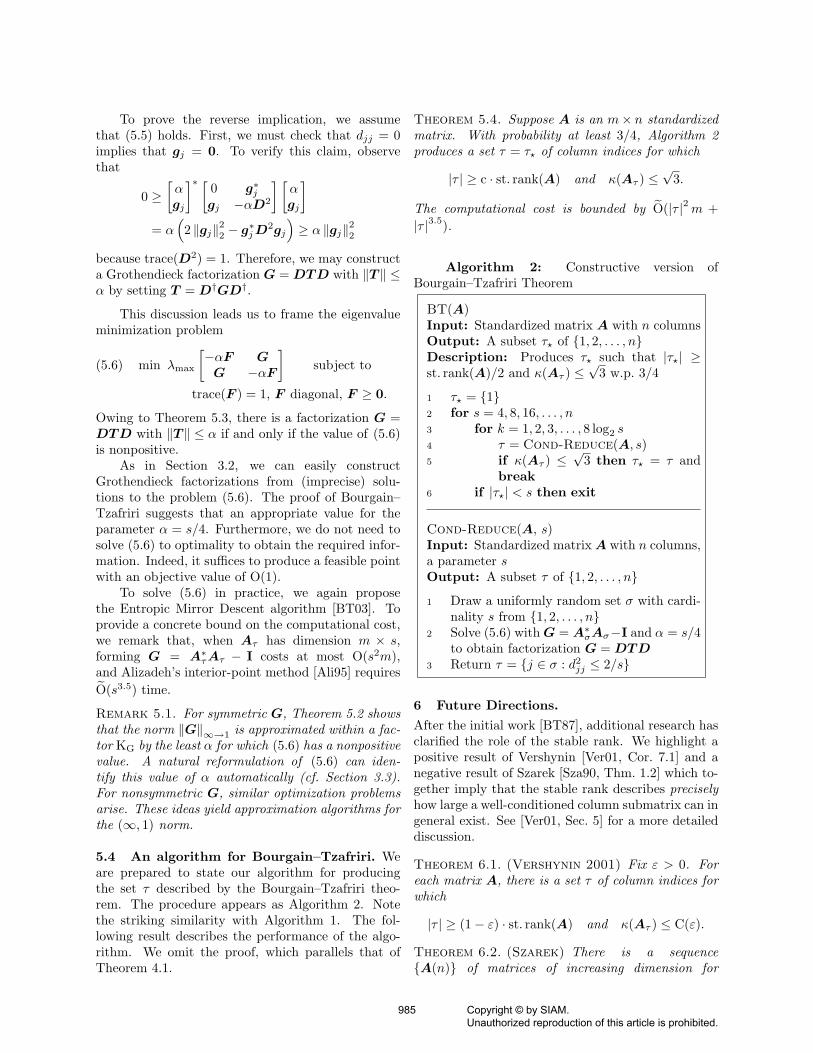
5.4 An algorithm for Bourgain–Tzafriri. Weare prepared to state our algorithm for producingthe set τ described by the Bourgain–Tzafriri theo-rem. The procedure appears as Algorithm 2. Notethe striking similarity with Algorithm 1. The fol-lowing result describes the performance of the algo-rithm. We omit the proof, which parallels that ofTheorem 4.1.

Theorem 5.4. Suppose A is an m× n standardizedmatrix. With probability at least 3/4, Algorithm 2produces a set τ = τ? of column indices for which

|τ | ≥ c · st. rank(A) and κ(Aτ ) ≤√

3.

The computational cost is bounded by O(|τ |2m +|τ |3.5).

Algorithm 2: Constructive version ofBourgain–Tzafriri Theorem

BT(A)Input: Standardized matrix A with n columnsOutput: A subset τ? of 1, 2, . . . , nDescription: Produces τ? such that |τ?| ≥st. rank(A)/2 and κ(Aτ ) ≤

√3 w.p. 3/4

1 τ? = 12 for s = 4, 8, 16, . . . , n3 for k = 1, 2, 3, . . . , 8 log2 s4 τ = Cond-Reduce(A, s)5 if κ(Aτ ) ≤

√3 then τ? = τ and

break6 if |τ?| < s then exit

Cond-Reduce(A, s)Input: Standardized matrix A with n columns,a parameter sOutput: A subset τ of 1, 2, . . . , n

1 Draw a uniformly random set σ with cardi-nality s from 1, 2, . . . , n

2 Solve (5.6) with G = A∗σAσ−I and α = s/4to obtain factorization G = DTD

3 Return τ = j ∈ σ : d2jj ≤ 2/s

6 Future Directions.

After the initial work [BT87], additional research hasclarified the role of the stable rank. We highlight apositive result of Vershynin [Ver01, Cor. 7.1] and anegative result of Szarek [Sza90, Thm. 1.2] which to-gether imply that the stable rank describes preciselyhow large a well-conditioned column submatrix can ingeneral exist. See [Ver01, Sec. 5] for a more detaileddiscussion.

Theorem 6.1. (Vershynin 2001) Fix ε > 0. Foreach matrix A, there is a set τ of column indices forwhich

|τ | ≥ (1− ε) · st. rank(A) and κ(Aτ ) ≤ C(ε).

Theorem 6.2. (Szarek) There is a sequenceA(n) of matrices of increasing dimension for

985 Copyright © by SIAM. Unauthorized reproduction of this article is prohibited.

which

|τ | = st. rank(A) =⇒ κ(Aτ ) = ω(1).

Vershynin’s proof constructs the set τ in Theo-rem 6.1 with a complicated iteration that interleavesthe Kashin–Tzafriri theorem and the Bourgain–Tzafriri theorem. We believe that the argument canbe simplified substantially and developed into a col-umn selection algorithm. This achievement mightlead to a new method for performing rank-revealingfactorizations, which could have a significant impacton the practice of numerical linear algebra.

Acknowledgments.

The author thanks Ben Recht for valuable discussionsabout eigenvalue minimization.

References

[Ali95] F. Alizadeh. Interior-point methods in semidefi-nite programming with applications to combinato-rial optimization. SIAM J. Optimization, 5(1):13–51, Feb. 1995.

[AN04] N. Alon and A. Naor. Approximating the cutnorm via Grothendieck’s inequality. In Proc. 36thAnn. ACM Symposium on Theory of Computing(STOC), pages 72–80, Chicago, 2004.

[BDM08] C. Boutsidis, P. Drineas, and M. Mahoney.On selecting exactly k columns from a matrix.Submitted for publication, 2008.

[BT87] J. Bourgain and L. Tzafriri. Invertibility of“large” submatrices with applications to the geom-etry of Banach spaces and harmonic analysis. IsraelJ. Math, 57(2):137–224, 1987.

[BT91] J. Bourgain and L. Tzafriri. On a problem ofKadison and Singer. J. reine angew. Math., 420:1–43, 1991.

[BT03] A. Beck and M. Teboulle. Mirror descent andnonlinear projected subgradient methods for convexoptimization. Operations Res. Lett., 31:167–175,2003.

[GE96] M. Gu and S. Eisenstat. Efficient algorithms forcomputing a strong rank-revealing QR factorization.SIAM J. Sci. Comput., 17(4):848–869, Jul. 1996.

[GW95] M. X. Goemans and D. P. Williamson. Improvedapproximation algorithms for maximum cut and sat-isfiability problems using semidefinite programming.J. Assoc. Comput. Mach., 42:1115–1145, 1995.

[HJ85] R. A. Horn and C. R. Johnson. Matrix Analysis.Cambridge Univ. Press, 1985.

[LO96] A. S. Lewis and M. L. Overton. Eigenvalueoptimization. Acta Numerica, 5:149–190, 1996.

[Pis86] G. Pisier. Factorization of linear operators andgeometry of Banach spaces. Number 60 in CBMSRegional Conference Series in Mathematics. AMS,Providence, 1986. Reprinted with corrections, 1987.

[Roh00] J. Rohn. Computing the norm ‖A‖∞,1 is NP-hard. Linear and Multilinear Algebra, 47:195–204,2000.

[RV07] M. Rudelson and R. Vershynin. Sampling fromlarge matrices: An approach through geomet-ric functional analysis. J. Amer. Comput. Soc.,54(4):Article 21, pp. 1–19, Jul. 2007.

[Sza90] S. Szarek. Spaces with large distance from `n∞

and random matrices. Amer. J. Math., 112(6):899–942, Dec. 1990.

[Tro08] J. A. Tropp. Column subset selection, matrixfactorization, and eigenvalue optimization. ACMTechnical Report 2008-02, California Institute ofTechnology, 2008.

[Ver01] R. Vershynin. Johns decompositions: Selecting alarge part. Israel J. Math., 122:253–277, 2001.

986 Copyright © by SIAM. Unauthorized reproduction of this article is prohibited.