Embed Size (px)
Citation preview
Combinatorial complexes, Bruhat intervals and
reflection distances
Axel Hultman
Stockholm 2003
Doctoral DissertationRoyal Institute of TechnologyDepartment of Mathematics

Akademisk avhandling som med tillstand av Kungl Tekniska Hogskolan framlag-ges till offentlig granskning for avlaggande av teknisk doktorsexamen tisdagen den21 oktober 2003 kl 15.15 i sal E2, Huvudbyggnaden, Kungl Tekniska Hogskolan,Lindstedtsvagen 3, Stockholm.
ISBN 91-7283-591-5TRITA-MAT-03-MA-16ISSN 1401-2278ISRN KTH/MAT/DA--03/07--SE
c© Axel Hultman, September 2003
Universitetsservice US AB, Stockholm 2003
Abstract
The various results presented in this thesis are naturally subdivided into three differ-ent topics, namely combinatorial complexes, Bruhat intervals and expectedreflection distances. Each topic is made up of one or several of the altogethersix papers that constitute the thesis. The following are some of our results, listedby topic:
Combinatorial complexes:
• Using a shellability argument, we compute the cohomology groups of the com-plements of polygraph arrangements. These are the subspace arrangementsthat were exploited by Mark Haiman in his proof of the n! theorem. We alsoextend these results to Dowling generalizations of polygraph arrangements.
• We consider certain B- and D-analogues of the quotient complex ∆(Πn)/Sn,i.e. the order complex of the partition lattice modulo the symmetric group,and some related complexes. Applying discrete Morse theory and an improvedversion of known lexicographic shellability techniques, we determine theirhomotopy types.
• Given a directed graph G, we study the complex of acyclic subgraphs of G aswell as the complex of not strongly connected subgraphs of G. Known resultsin the case of G being the complete graph are generalized.
Bruhat intervals:We list the (isomorphism classes of) posets that appear as intervals of length 4
in the Bruhat order on some Weyl group. In the special case of symmetric groups,we list all occuring intervals of lengths 4 and 5.
Expected reflection distances:Consider a random walk in the Cayley graph of the complex reflection group
G(r, 1, n) with respect to the generating set of reflections. We determine the ex-pected distance from the starting point after t steps. The symmetric group case(r = 1) has bearing on the biologist’s problem of computing evolutionary distancesbetween different genomes. More precisely, it is a good approximation of the ex-pected reversal distance between a genome and the genome with t random reversalsapplied to it.
ISBN 91-7283-591-5 • TRITA-MAT-03-MA-16 • ISSN 1401-2278 • ISRN KTH/MAT/DA--03/07--SE
iii

iv
Preface
If you are a mathematician, then you know all too well the following question: “But,what does a mathematician really do?”. Luckily, thanks to Pal Erdos, we all knowthe proper answer: mathematicians convert coffee into theorems. However, somepeople are rather persistent and keep going: “But, what is a theorem anyway?”.The answer is, of course, that a theorem is a tautology, a way to rephrase something.It doesn’t say anything new! Thus, mathematics is basically the art of convertingcoffee into nothing, which is, clearly, to violate the first law of thermodynamics.This, of course, must never be told to the people that fund us.
During my graduate studies, a range of helpful people have guided and aidedmy attempts to violate the first law of thermodynamics. Among them are thefollowing:
• Anders Bjorner has been a superb advisor. Being an enormously rich sourceof advice and hints, of answers and questions, of ideas and suggestions, hehas provided the best possible support a graduate student can hope for.
• Kimmo Eriksson helped me excellently through the first part of my graduatestudies, while Anders was ill. He also carefully read the article which hasbecome Paper 5 of this thesis.
• After Kimmo had left for Malardalen University, Dmitry Kozlov was kindenough to take his place. Apart from being ever helpful, he guided me throughwriting my first paper, which forms Paper 2 of this thesis.
• Through a large portion of my time as a graduate student, Niklas Eriksenwas the only other combinatorics student at the department. We had manyinteresting discussions, and we wrote two articles together. They form Papers5 and 6 of this thesis. Niklas also filled the important position as organizerof the department’s weekly floorball matches.
• Niklas and I tried for some time to prove a crucial result (Theorem 5.5.1)without success. We then asked Richard Stanley of MIT for advice. Hereplied with the solution virtually before we had even asked the question.
v

vi Preface
• The entire staff of the department has provided a helpful and friendly envi-ronment suitable to work in.
• Finally, the people who have helped me the most (although the majoritycouldn’t care less about mathematics!), and without whom I would neverhave had the opportunity nor the energy to work on this thesis, are my ever-supportive family and friends. You know who you are.
Contents
Introduction 10.1 Combinatorial complexes . . . . . . . . . . . . . . . . . . . . . . . 1
0.1.1 Subspace arrangements and shellability . . . . . . . . . . . 20.1.2 Boolean cell complexes . . . . . . . . . . . . . . . . . . . . . 30.1.3 Graph complexes . . . . . . . . . . . . . . . . . . . . . . . . 4
0.2 Bruhat intervals . . . . . . . . . . . . . . . . . . . . . . . . . . . . 40.3 Expected reflection distances . . . . . . . . . . . . . . . . . . . . . 50.4 Overview of the papers . . . . . . . . . . . . . . . . . . . . . . . . . 6
I Combinatorial complexes 9
Paper 1. Polygraph arrangements. 11
1.1 Introduction . . . . . . . . . . . . . . . . . . . . . . . . . . . . . . . 111.2 Tools for investigation of subspace arrangements . . . . . . . . . . 121.2.1 The Goresky-MacPherson formula . . . . . . . . . . . . . . 121.2.2 Lexicographic shellings . . . . . . . . . . . . . . . . . . . . . 13
1.3 Polygraph arrangements . . . . . . . . . . . . . . . . . . . . . . . . 131.4 An EL-labelling of L(Q,P ) . . . . . . . . . . . . . . . . . . . . . . 141.5 A Dowling generalization . . . . . . . . . . . . . . . . . . . . . . . 18
1.5.1 Dowling lattices . . . . . . . . . . . . . . . . . . . . . . . . 181.5.2 Dowling analogues of L(Q, P ) . . . . . . . . . . . . . . . . . 19
Paper 2. Quotient complexes and lexicographic shellability. 252.1 Introduction . . . . . . . . . . . . . . . . . . . . . . . . . . . . . . . 252.2 Basic definitions and notation . . . . . . . . . . . . . . . . . . . . . 26
2.2.1 Shelling cell complexes of boolean type . . . . . . . . . . . . 262.2.2 Discrete Morse theory . . . . . . . . . . . . . . . . . . . . . 272.2.3 Quotient complexes . . . . . . . . . . . . . . . . . . . . . . 27
2.3 Lexicographic shellability of balanced boolean cell complexes . . . 282.4 The objects of study . . . . . . . . . . . . . . . . . . . . . . . . . . 312.5 Describing ∆n,k,h using trees . . . . . . . . . . . . . . . . . . . . . 32
vii
viii Contents
2.5.1 The trees . . . . . . . . . . . . . . . . . . . . . . . . . . . . 332.5.2 The deletion operator . . . . . . . . . . . . . . . . . . . . . 342.5.3 A description of ∆n,k,h . . . . . . . . . . . . . . . . . . . . . 34
2.6 The homotopy type of ∆n,k,h . . . . . . . . . . . . . . . . . . . . . 342.6.1 The Dn,k case . . . . . . . . . . . . . . . . . . . . . . . . . . 352.6.2 The Bn,k,h case . . . . . . . . . . . . . . . . . . . . . . . . . 36
Paper 3. Directed subgraph complexes. 413.1 Introduction . . . . . . . . . . . . . . . . . . . . . . . . . . . . . . . 413.2 Basic topological combinatorics . . . . . . . . . . . . . . . . . . . . 423.3 Acyclic subgraphs . . . . . . . . . . . . . . . . . . . . . . . . . . . 433.4 Not strongly connected subgraphs . . . . . . . . . . . . . . . . . . 44
II Bruhat intervals 49
Paper 4. Bruhat intervals of length 4 in Weyl groups. 514.1 Introduction . . . . . . . . . . . . . . . . . . . . . . . . . . . . . . . 514.2 Foundations . . . . . . . . . . . . . . . . . . . . . . . . . . . . . . . 524.3 Classifying the intervals of length 4 . . . . . . . . . . . . . . . . . . 55
4.3.1 Crown indices . . . . . . . . . . . . . . . . . . . . . . . . . . 554.3.2 Cell decompositions of the 2-sphere . . . . . . . . . . . . . . 564.3.3 The classification . . . . . . . . . . . . . . . . . . . . . . . . 58
4.4 A completely computerized approach . . . . . . . . . . . . . . . . . 65
Complement. Bruhat intervals of length 5 in symmetric groups 674.5 More computer calculations . . . . . . . . . . . . . . . . . . . . . . 67
III Expected reflection distances 73
Paper 5. Estimating the expected reversal distance after t randomreversals. 755.1 Introduction . . . . . . . . . . . . . . . . . . . . . . . . . . . . . . . 755.2 Preliminaries . . . . . . . . . . . . . . . . . . . . . . . . . . . . . . 76
5.2.1 The cycle graph . . . . . . . . . . . . . . . . . . . . . . . . 775.3 The analogy . . . . . . . . . . . . . . . . . . . . . . . . . . . . . . . 795.4 The Markov chain approach . . . . . . . . . . . . . . . . . . . . . . 805.5 Decomposing the length function . . . . . . . . . . . . . . . . . . . 83
5.5.1 Proof of Theorem 5.4.3 . . . . . . . . . . . . . . . . . . . . 855.5.2 Computing the variance . . . . . . . . . . . . . . . . . . . . 85
5.6 Experimental results . . . . . . . . . . . . . . . . . . . . . . . . . . 865.6.1 Predicting the true reversal distance . . . . . . . . . . . . . 86
5.7 Conclusions . . . . . . . . . . . . . . . . . . . . . . . . . . . . . . . 87
Contents ix
Paper 6. Expected reflection distance in G(r, 1, n) after t randomreflections. 896.1 Introduction . . . . . . . . . . . . . . . . . . . . . . . . . . . . . . . 896.2 The group G(r, 1, n) and its reflection graph . . . . . . . . . . . . . 906.3 Irreducible characters and “symmetric functions” . . . . . . . . . . 916.4 The Markov chain . . . . . . . . . . . . . . . . . . . . . . . . . . . 926.5 The eigenvalues of the adjacency matrices . . . . . . . . . . . . . . 956.6 Decomposing the distance function . . . . . . . . . . . . . . . . . . 976.7 Proof of Theorem 6.4.2 . . . . . . . . . . . . . . . . . . . . . . . . . 101

x
Introduction
This thesis consists of six different papers. There are ways to tie all of themtogether. For instance, the symmetric group and its relatives play important rolesin all of the papers. However, a less artificial and more natural point of view isprobably to divide the papers into three different categories:
• Combinatorial complexes. This category includes the first three papers,which all deal with topological properties of combinatorially defined cell com-plexes.
• Bruhat intervals. Paper 4 and a complement to it are the only members ofthis category. They address the problem of characterizing those posets thatoccur as intervals in Bruhat orders of Weyl groups.
• Expected reflection distances. The remainder of the thesis, Papers 5and 6, concern expected distances after random walks on Cayley graphs ofreflection groups.
Any of the above categories is mostly independent of the others. Below, we thusgive an independent introduction to each. We will assume some knowledge ofcombinatorics, topology, Coxeter groups and complex reflection groups. We referto [69], [62], [50] and [67], respectively, for more on these subjects.
0.1 Combinatorial complexes
Among the various classes of cell complexes, the most fundamental and importantis probably the class of simplicial complexes. Viewing a simplicial complex as anabstract complex, i.e. as a collection of sets which is closed under taking subsets, itis clear that simplicial complexes are indeed very combinatorial by nature. On theother hand, viewing a complex as its geometric realization, it has a distinct topo-logical flavour. Exploiting this connection between topology and combinatorics,the following question has often turned out to be highly interesting: “What are thetopological properties of this combinatorially defined simplicial complex?”.
A fundamental construction in this area is the order complex ∆(P ) of a posetP . It is the simplicial complex whose faces are the chains in P . Thus, to any
1
2 Introduction
poset we may associate topological properties. Moreover, the topological propertiesare closely connected to the combinatorics of the poset. The Mobius function ofan interval, for instance, coincides with the reduced Euler characteristic of theorder complex of the interval with 0 and 1 removed. (As is customary, we use theconvention that the unique maximal and minimal elements of a poset are denoted0 and 1, respectively, if they exist.)
0.1.1 Subspace arrangements and shellability
One nice application of order complexes belongs to the theory of subspace arrange-ments. A (real) subspace arrangement is a collection of linear subspaces of Euclideanspace Rn. To an arrangement A, one associates the intersection lattice L(A). Itconsists of all possible intersections of subsets of A ordered by reverse inclusion.An interesting topological space related to A is its complement MA = Rn \ ∪A.Goresky and MacPherson [39] showed that the cohomology groups of MA can becomputed from the homology groups of the open lower intervals of L(A):
Theorem 0.1.1 (The Goresky-MacPherson formula). For all i,
Hi(MA;Z) ∼=⊕
x∈L(A)\0HcodimR(x)−i−2(∆((0, x));Z)
In order to apply Theorem 0.1.1, one clearly has to get a grip on the homologyof the order complexes of various posets, namely the open lower intervals in theintersection lattice. If this lattice is well-behaved enough, it may be worthwhile totry one of the various lexicographic shellability techniques. We now describe themost commonly used of them, namely EL-shellability. It was introduced in [6] forgraded posets and generalized to non-graded posets in [16].
A bounded poset is one equipped with 0 and 1. We also use the notation P =P \ 0, 1 to denote the proper part of P if P is bounded. Similarly, if P is anyposet, then P denotes the bounded poset obtained by adjoining a top and a bottomelement, 0 and 1, to P .
We write x → y if y covers x in P , and let R(P ) denote the covering relation,which can be thought of as the set of edges in the Hasse diagram of P . Therefore,a map λ : R(P ) → Λ is called an edge labelling of P . Here, Λ is a poset whoseelements we think of as labels.
Given an edge labelling λ, a saturated chain x = (x0 → x1 → · · · → xk) isrising if λ(xi−1 → xi) < λ(xi → xi+1) for all i ∈ [k − 1]. It is falling if, instead,λ(xi−1 → xi) 6< λ(xi → xi+1) for all i. Letting λ(x) denote the sequence (λ(x0 →x1), . . . , λ(xk−1 → xk)), we compare two saturated chains x and y with commonendpoints using the lexicographic partial order induced by Λ on the sequences λ(x)and λ(y).
Definition 0.1.2. Suppose that P is bounded. An edge labelling λ : R(P ) → Λ iscalled an EL-labelling if the following two conditions hold for all pairs p < q in P .

0.1. Combinatorial complexes 3
• There is a unique rising saturated chain from p to q.
• The unique rising chain is lexicographically smaller than every other saturatedchain from p to q.
If P has an EL-labelling, then P is called EL-shellable.
If P is EL-shellable, then so is, clearly, every interval in P . The followingtheorem thus provides the information needed to apply the Goresky-MacPhersonformula if the intersection lattice is EL-shellable.
Theorem 0.1.3 (see [6, 16]). If P is EL-shellable, then ∆(P ) is homotopy equiv-alent to a wedge of spheres. The number of i-dimensional spheres in the wedgeequals the number of maximal chains in P that have exactly i + 3 elements.
In [42], Haiman introduced a class of subspace arrangements, called polygrapharrangements, whose algebraic properties he exploited in his proof of the celebratedn! theorem. In Paper 1, we apply the Goresky-MacPherson formula to computethe cohomology of the complement of these and some more general arrangements.We achieve this by showing that their intersection lattices are EL-shellable.
0.1.2 Boolean cell complexes
To a regular CW complex ∆, we associate the face poset P (∆). It consists of thefaces of ∆ ordered by inclusion. If ∆ is simplicial, then every interval in P (∆) is aboolean algebra. In fact, a poset, equipped with 0, whose every interval is a booleanalgebra is called a simplicial poset. The class of complexes with simplicial posetsas face posets is, however, a little broader; such complexes are called cell complexesof boolean type, or boolean cell complexes for short, and were introduced by Bjorner[8] and by Garsia and Stanton [36]. Note that in a boolean cell complex, severalcells may share the same set of vertices.
An interesting way to construct boolean cell complexes is the following. Supposethat G is a group which acts order-preservingly on a poset P . Then, we canconstruct the quotient complex ∆(P )/G. It is a boolean cell complex whose cellsare the G-orbits of faces in ∆(P ). One reason to be interested in this complex isits connection to representation theory. More precisely, it follows e.g. from Bredon[19], that the multiplicity of the trivial character in the induced G-representationon the ith homology group of ∆(P ) equals the rank of the ith homology group of∆(P )/G (unless we have coefficients in a field of “bad” positive characteristic).
Kozlov [56] studied the quotient construction for the case of the symmetricgroup Sn acting on the (proper part of the) partition lattice Πn as well as on moregeneral lattices. He showed that the resulting quotient complex is collapsible. InCoxeter group terminology, this quotient complex can be thought of as a type Aconstruction. In Paper 2, we obtain B- and D-analogues of Kozlov’s results. In theprocess, we describe and use a new lexicographic shellability technique for a classof boolean cell complexes. It generalizes the non-pure CL-shellability of Bjorner
4 Introduction
and Wachs [16] beyond posets. It is very closely related to the technique for pureboolean cell complexes developed by Hersh [45].
0.1.3 Graph complexes
So far, the “combinatoriality” of the combinatorial complexes that we have con-sidered has been inherited from some underlying poset. A different class of con-structions has to do with graph properties. A property of (directed or undirected)graphs is called monotone if it is preserved under deletion of edges. For instance,the property “forest” is monotone, whereas the property “tree” is not. Given n ∈ Nand a monotone graph property P , we may define a simplicial complex ∆P
n . Itssimplices are the edge sets of graphs on vertex set [n] that satisfy P . We refer to∆P
n as the complex of graphs satisfying P .In a recent upsurge of activity in this area, this construction has been studied
for numerous properties P . Examples include complexes of not i-connected graphs[2, 53, 74], i-colorable graphs [58], directed forests [18, 55], matchings [75], graphsof bounded degree [24, 75], and so on.
Fixing P and a graph G, a more general construction than ∆Pn is obtained by
letting ∆PG be the complex of all subgraphs of G that satisfy P . In Paper 3, we
study directed subgraph complexes of this type using the properties acyclicity andstrong non-connectivity. Bjorner and Welker [18] did this in the case of all graphs,and basically we adapt their techniques in order to generalize their results.
0.2 Bruhat intervals
The Bruhat order is a partial order defined on any Coxeter group. It arises in amultitude of contexts; for example, it records the incidences between closed Schu-bert cells for a reductive algebraic group over an algebraically closed field. It maybe defined, though, in a highly combinatorial manner.
Let (W,S) be a Coxeter system with reflection set T and length function `.
Definition 0.2.1. The Bruhat order on W is the partial order defined by
u ≤ w iff there exist t1, . . . , tj ∈ T such that w = ut1 . . . tj
and `(ut1 . . . ti) < `(ut1 . . . ti+1) for all i.
Although not obvious from Definition 0.2.1, the Bruhat order is a graded posetwith ` as rank function. It is well-known (see e.g. [12]) that there are infinitely manyranked posets of length 3 that appear as intervals in Bruhat orders on infiniteCoxeter groups. In [7], on the other hand, Bjorner asked if only finitely manyposets of each fixed length are Bruhat intervals in finite Coxeter groups. Dyer [28]answered Bjorner’s question affirmatively. Thus, the following problem is natural:“List the posets, of each fixed length, that are Bruhat intervals in finite Coxetergroups.”. The answers for lengths 2 and 3 follow e.g. from [15] together with any
0.3. Expected reflection distances 5
table of Kazhdan-Lusztig polynomials, for instance [38]. In length 2, the “diamond-shaped” poset is the only possibility, whereas in length 3, the face posets of k-gons,k ∈ 2, 3, 4, 5, are the four available options (see Figure 4.3).
In Paper 4, we list the Bruhat intervals of length 4 that appear in Weyl groups,and in a complement to Paper 4 we list the Bruhat intervals of length 5 thatappear in symmetric groups. Our method is to find the intervals that occur inWeyl groups of rank at most 4 through a combination of computer calculations andtheoretical arguments. We also do the same thing using an independent, completelycomputerized, approach, which we (in the aforementioned complement) also applyto the symmetric group A5. This suffices since, by a result of Dyer [28] and ourLemma 4.2.6, if a poset is a Bruhat interval of length i in a particular class ofCoxeter groups, then it must occur already in a group of rank at most i in the sameclass. The applicable classes include finite Coxeter groups, Weyl groups, simply-laced Weyl groups and direct products of symmetric groups.
0.3 Expected reflection distances
Consider the Cayley graph of the symmetric group Sn with respect to the generatingset of transpositions. A random walker starts walking from the identity. At eachstep, he moves along one of the edges incident to his current position, randomlychosen with equal probability. How far away from the identity do we expect himto be after t steps?
One motivation to study this problem comes from computational biology. Onemodel for evolution among biologists is that genomes are subject to reversals, mu-tations that modify genomes in a prescribed fashion. Thus, applying random re-versals to a genome is thought to simulate evolution. As we justify in Paper 5,a random walk in the Cayley graph described above is for many purposes a goodapproximation.
Together with Niklas Eriksen, we present a solution to our problem in the papercited above. In other words, we give a formula for the expected transpositiondistance of a product of t random transpositions in Sn. It turns out that, usingresults of Ito [51] and some manipulations, our problem is equivalent to finding theexplicit decomposition of the class function ` (which sends an integer partition toits number of parts) into irreducible Sn-characters. Generously aided by RichardStanley, we apply tools from the theory of symmetric functions to determine thisdecomposition.
The symmetric group Sn is the r = 1 member of the family G(r, 1, n) of complexreflection groups. (Another way to view G(r, 1, n) is as the wreath product Zr oSn,where Zr is the cyclic group on r elements.) The transpositions in Sn are thenreplaced by the (complex) reflections in G(r, 1, n). Again together with NiklasEriksen, we generalize the mathematical results of Paper 5 from Sn to G(r, 1, n)in Paper 6. In particular, when r = 2, we provide B-analogues. Our approach is
6 Introduction
basically the same as in Paper 5, although the representation theory of G(r, 1, n),when r > 1, provides some additional obstacles.
0.4 Overview of the papers
Here, we give a brief overview of the six papers that constitute this thesis.
1. Polygraph arrangements.(Based on [47], published in European Journal of Combinatorics.)
A class of subspace arrangements, Z(n,m), known as polygraph arrangementswas exploited by Haiman in order to prove the n! theorem. By showing thattheir intersection lattices, L(Z(n,m)), are EL-shellable, we determine thecohomology groups of the complements of the arrangements. Moreover, wegeneralize the shellability results to a class of lattices which deserve to becalled Dowling generalizations of L(Z(n,m)). As a consequence, we obtainthe cohomology groups of the complements of certain Dowling analogues ofpolygraph arrangements.
2. Quotient complexes and lexicographic shellability.(Based on [46], published in Journal of Algebraic Combinatorics.)
Let Πn,k,k and Πn,k,h, h < k, denote the intersection lattices of the k-equalsubspace arrangement of type Dn and the k, h-equal subspace arrangementof type Bn respectively. Denote by SB
n the group of signed permutations. Weshow that ∆(Πn,k,k)/SB
n is collapsible. For ∆(Πn,k,h)/SBn , h < k, we show
the following. If n ≡ 0 (mod k), then it is homotopy equivalent to a sphere ofdimension 2n
k −2. If n ≡ h (mod k), then it is homotopy equivalent to a sphereof dimension 2n−h
k −1. Otherwise, it is contractible. Immediate consequencesfor the multiplicity of the trivial characters in the representations of SB
n onthe homology groups of ∆(Πn,k,k) and ∆(Πn,k,h) are stated.
The collapsibility of ∆(Πn,k,k)/SBn is established using a discrete Morse func-
tion. The same method is used to show that ∆(Πn,k,h)/SBn , h < k, is ho-
motopy equivalent to a certain subcomplex. The homotopy type of this sub-complex is calculated by showing that it is shellable. To do this, we are ledto introduce a lexicographic shelling condition for balanced cell complexes ofboolean type. This extends to the non-pure case work of Hersh [45] and spe-cializes to the CL-shellability of Bjorner and Wachs [16] when the cell complexis an order complex of a poset.
3. Directed subgraph complexes.(Based on [48], unpublished.)
0.4. Overview of the papers 7
Let G be a directed graph, and let ∆ACYG be the simplicial complex whose sim-
plices are the edge sets of acyclic subgraphs of G. Similarly, we define ∆NSCG
to be the simplicial complex with the edge sets of not strongly connected sub-graphs of G as simplices. We show that ∆ACY
G is homotopy equivalent to the(n−1−k)-dimensional sphere if G is a disjoint union of k strongly connectedgraphs. Otherwise, it is contractible. If G belongs to a certain class of graphs,the homotopy type of ∆NSC
G is shown to be a wedge of (2n− 4)-dimensionalspheres. The number of spheres can easily be read off the chromatic polyno-mial of a certain associated undirected graph.
4. Bruhat intervals of length 4 in Weyl groups.(Based on [49], published in Journal of Combinatorial Theory, Series A.)
We determine all isomorphism classes of intervals of length 4 in the Bruhatorder on the Weyl groups A4, B4, D4 and F4. It turns out that there are 24of them (some of which are dual to each other). Work of Dyer allows us toconclude that these are the only intervals of length 4 that can occur in theBruhat order on any Weyl group. We also determine the intervals that arisealready in the smaller classes of simply-laced Weyl groups and symmetricgroups.
Our method combines theoretical arguments and computer calculations. Wealso present an independent, completely computerized, approach.
Complement. (Not included in [49].) The completely computerized ap-proach is applied to find all intervals of length 5 in A5. The 25 posets thatare found are the only intervals of length 5 that appear in Bruhat orders onsymmetric groups.
5. Estimating the expected reversal distance after t random reversals.(With N. Eriksen, based on [31], accepted for publication in Advances inApplied Mathematics.)
We address the problem of computing the expected reversal distance of agenome with n genes obtained by applying t random reversals to the identitygenome. A good approximation is the expected transposition distance of aproduct of t random transpositions in Sn. Computing the latter turns outto be equivalent to computing the coefficients of the length function (i.e. theclass function returning the number of parts in an integer partition) whenwritten as a linear combination of the irreducible characters of Sn. Usingsymmetric functions theory, we compute these coefficients, thus obtaining aformula for the expected transposition distance. We also briefly sketch howto compute the variance.

8 Introduction
6. Expected reflection distance in G(r, 1, n) after t random reflections.(With N. Eriksen, based on [32], unpublished.)
Extending to r > 1 the formula for the expected transposition distance men-tioned above, we compute the expected reflection distance of a product oft random reflections in the complex reflection group G(r, 1, n). The resultrelies on an explicit decomposition of the reflection distance function intoirreducible G(r, 1, n)-characters and on the eigenvalues of certain adjacencymatrices.

Part I
Combinatorial complexes
9

10
Paper 1.
Polygraph arrangements
1.1 Introduction
Macdonald [59] introduced a family of polynomials known as Macdonald polynomi-als. They constitute a basis of the algebra of symmetric functions in the variablesx1, x2, . . . with coefficients in the field of fractions of Q[y, z]. Transformation to thebasis of Schur functions gives rise to transition coefficients that are called Kostka-Macdonald coefficients. Until recently, the conjecture that the Kostka-Macdonaldcoefficients in fact are polynomials in y and z with nonnegative integer coefficientswas open. This conjecture was known as the Macdonald positivity conjecture.
Garsia and Haiman [35] conjectured that the Kostka-Macdonald coefficientsare multiplicities of graded characters of certain Sn-modules. An equivalent (seeHaiman [42]) formulation of this has become known as the n! conjecture, sinceit asserts that the said modules are of dimension n!. This implies the positivityconjecture.
Recently, Haiman [41] proved the n! conjecture. The proof relies on the fact thata class of subspace arrangements in (C2)n+m, called polygraph arrangements, havecoordinate rings that are free modules over the polynomial ring in one coordinateset on (C2)n.
In this paper, we show that certain lattices, which deserve to be called Dowlinggeneralizations of the intersection lattices of the polygraph arrangements, are EL-shellable. Via the Goresky-MacPherson formula, this allows us to determine thecohomology groups of the complements of the polygraph arrangements as well asof Dowling analogues of these arrangements. In particular, it turns out that thecohomology is free and vanishing in “most” dimensions.
The structure of this paper is as follows. After briefly reviewing basic definitionsand tools in Section 1.2, we deal with the case of ordinary polygraph arrangementsin Sections 1.3 and 1.4. In Section 1.5, we give Dowling generalizations of theresults in Section 1.4.
11
12 Paper 1. Polygraph arrangements
The proofs of Section 1.5 certainly specialize to proofs of the theorems in Section1.4. However, they do not quite specialize to the proofs given in Section 1.4; thelatter are simpler and more transparent. This is the reason why we treat ordinarypolygraph arrangements and their Dowling generalizations separately.
Acknowledgement. The author is grateful to his advisor Anders Bjorner whosuggested the study of polygraph arrangements. Moreover, his careful reading andremarks have led to substantial improvements in the paper.
1.2 Tools for investigation of subspace arrange-ments
We give a brief survey of the techniques that are used in this paper. For basiccombinatorial and topological concepts, the reader is referred to the textbooksby Stanley [68] and Munkres [62]. For more on subspace arrangements, see e.g.Bjorner’s survey article [9].
A subspace arrangement is a collection A = A1, . . . , An of affine subspacesof km, where k is some field. In case k ∈ R,C, one is often interested in thetopological features of the complement MA := km \ (
⋃ni=1 Ai).
1.2.1 The Goresky-MacPherson formula
To any poset P , we associate the order complex ∆(P ). This is the simplicial complexhaving the chains of P as simplices. If P has a bottom and/or a top element, thenthe symbols 0 and 1 will be used to denote them, respectively. The proper part Pis the poset P \ 0, 1.
The intersection semi-lattice L(A) of A is the meet semi-lattice of all nonemptyintersections of subsets of A ordered by reverse inclusion. It is a lattice iff
⋂ni=1 Ai 6=
∅. In case k ∈ R,C, the following result of Goresky and MacPherson [39] relatesthe reduced cohomology groups of MA and the reduced homology of the lowerintervals of L(A):
Theorem 1.2.1. (The Goresky-MacPherson formula) Let A be a real subspacearrangement (i.e. k = R). Then, for all i,
Hi(MA;Z) ∼=⊕
x∈L(A)\0HcodimR(x)−i−2(∆([0, x]);Z).
Note that we can apply Theorem 1.2.1 to complex arrangements by identifyingC with R2. Then codimR(·) is replaced by 2codimC(·).
1.3. Polygraph arrangements 13
1.2.2 Lexicographic shellings
If we are interested in the cohomology of MA, then Theorem 1.2.1 leaves us withthe task of determining the homology of L(A) and its lower intervals. To thisend, the technique of EL-shellability described below will be useful to us. It wasintroduced for ranked posets by Bjorner [6] and later extended to arbitrary posetsby Bjorner and Wachs [16].
For a ranked poset P , let P denote the poset obtained by adding an additionaltop element 1 and an additional bottom element 0 to P . Let R(P ) ⊂ P 2 denotethe covering relation of P . We write x → y if y covers x. An edge-labelling ofP is a map λ : R(P ) → Λ, where Λ is some poset of labels. A saturated chainc = c1 → . . . → ct ⊆ P is rising if λ(c1 → c2) < · · · < λ(ct−1 → ct). Thechain c is falling if, instead, λ(c1 → c2) 6< · · · 6< λ(ct−1 → ct). Given an interval[x, y] ⊆ P , we compare two saturated chains c = x = c1 → . . . → ct = y andd = x = d1 → . . . → dt = y using the lexicographic order induced by Λ on thesequences λ(c1 → c2), . . . , λ(ct−1 → ct) and λ(d1 → d2), . . . , λ(dt−1 → dt).
Definition 1.2.2. λ : R(P ) → Λ is an EL-labelling of P if every P -intervalcontains a unique rising saturated chain and this chain is lexicographically smallerthan every other saturated chain in the interval. If P admits an EL-labelling, thenP is called EL-shellable.
Clearly, if P is EL-shellable, then so is every interval of P . Moreover, thehomotopy type of ∆(P ) can be read off the labelling:
Theorem 1.2.3. Suppose P is ranked of length i. If P has an EL-labelling, then∆(P ) is homotopy equivalent to a wedge of (i−2)-dimensional spheres. The spheresin the wedge are indexed by the falling maximal chains.
1.3 Polygraph arrangements
Now we describe our main objects of study. Let V be a d-dimensional vector spaceover k. For m,n ∈ N and a function f : [m] → [n], we let
Wf = (xf(1), . . . , xf(m), x1, . . . , xn) ∈ V m+n | xi ∈ V ∀i ∈ [n].This is a linear subspace of V m+n. The polygraph arrangement, ZV (n,m), is thecollection of all such subspaces:
ZV (n, m) := Wf | f : [m] → [n].Often, the choice of V (and k) is not important. Therefore, we frequently writeZ(n, m) instead of ZV (n, m). To avoid confusion, we mention that Haiman [41] letsZ(n, m) denote the union, not just the collection, of all Wf .
Note that ZV (n,m) is an arrangement of nm subspaces of dimension nd in the(m + n)d-dimensional vector space V m+n. The dimensions of all intersections ofsuch subspaces are divisible by d.
14 Paper 1. Polygraph arrangements
We need a combinatorial description of the intersection lattice L(Z(n,m)). Fromnow on, we let P = p1 < · · · < pm and Q = q1 < · · · < qn be fixed disjointordered sets. For a subset S ⊆ P ∪ Q, we use the notation SP := S ∩ P andSQ := S ∩ Q, so that S = SP ∪ SQ. Consider the following lattice, which is ajoin-subsemilattice of the partition lattice ΠP∪Q.
L(Q,P ) :=π1| . . . |πt ∈ ΠP∪Q | πPi = ∅ ⇒ |πQ
i | = 1
and πPi 6= ∅ ⇒ πQ
i 6= ∅ ∀i ∈ [t] ∪ 0.
Proposition 1.3.1. L(Z(n,m)) and L(Q,P ) are isomorphic.
Proof. Pick a subset F ⊆ f : [m] → [n]. The element⋂
f∈F Wf ∈ L(Z(n,m))can be represented by a bipartite graph GF = (P ∪ Q,E), where pi, qj ∈ E ifff(i) = j for some f ∈ F . Two such graphs represent the same subspace of V m+n
precisely if they have the same connected components. Clearly, all bipartite graphson P ∪Q in which deg(pi) ≥ 1 for all i ∈ [m] occur in this way. Thus, L(Z(n,m))is isomorphic to the lattice of partitions of P ∪ Q whose non-minimal elementscorrespond to connected components in bipartite graphs on P ∪Q with no isolatedvertices in P . This is precisely L(Q,P ).
Corollary 1.3.2. The intersection lattice L(Z(n,m)) is ranked of length n.
1.4 An EL-labelling of L(Q, P )
We will give an edge-labelling λ of L(Q,P ). It will turn out to be an EL-labelling.Our poset Λ of labels consists of four different types of labels: Ax-, Bx- and Cx-labels are ordered internally with respect to their indices. The fourth type is theset [n]m which is ordered lexicographically. The order on the different types isA < B < [n]m < C. More explicitly, we define
Λ = A2 < · · · < An < B1 < · · · < Bn < 11 . . . 11︸ ︷︷ ︸m
< 11 . . . 12︸ ︷︷ ︸m
< · · · < nn . . . n︸ ︷︷ ︸m
<
C2 < · · · < Cn.
The labelling λ : R(L(Q, P )) → Λ is defined by:
• λ(π → τ) = Ax if two non-singleton blocks, πi and πj , in π are merged in τ
and qx = max(πQi ∪ πQ
j ).
• λ(π → τ) = Bx if a singleton, qx, and a non-singleton block, πi, in π aremerged in τ and qx < max(πQ
i ).
• λ(π → τ) = Cx if a singleton, qx, and a non-singleton block, πi, in π aremerged in τ and qx > max(πQ
i ).
1.4. An EL-labelling of L(Q,P ) 15
• λ(0 → τ) = f(1)f(2) . . . f(m) (juxtapositioning) if τ corresponds to the sub-space Wf .
Theorem 1.4.1. The labelling λ is an EL-labelling of L(Q,P ).
Proof. Pick an interval I = [π, τ ] ⊆ L(Q, P ). We must verify that I contains aunique rising chain and that this chain is lexicographically least in I.
Suppose, to begin with, that π 6= 0. If there are non-singleton blocks in π whichare merged in τ , then any rising chain must begin with the merging of these blocks.This gives rise to A-labels, and for the subscripts of these labels to form a risingsequence, the order in which to merge the blocks is unique. Next, all singletonsqi that are to be merged with non-singleton blocks containing some qj > qi mustbe so. This gives rise to B-labels, and again there is a unique way to make theirsubscripts form a rising sequence. Finally, the remaining singletons that are largerthan all Q-elements in their blocks in τ are to be merged, this giving rise to C-labels.Once again, there is a unique order in which to do this within a rising chain. Thus,we have constructed the unique rising chain in I. Note that if we had replacedthe word rising with the phrase lexicographically least, then the above constructionwould give us the unique lexicographically least chain. Hence, it coincides with therising chain.
Now, suppose that π = 0. Note that I contains exactly one atom af , corre-sponding to the subspace Wf , with the property that [af , τ ] contains a chain withonly C-labels. The function f sends i ∈ [m] to the least j ∈ [n] such that pi andqj are in the same block in τ . As before, the C-labels occur with rising subscriptsin exactly one chain in [af , τ ]. Note that λ(0 → af ) < λ(0 → a) for all atomsa ∈ I \ af. Hence, the rising chain is again lexicographically least in I.
Remark. Let r = (r1, . . . , rm) ∈ [n]m. Haiman [43] has considered the subar-rangement Z(n,m, r) ⊆ Z(n,m) which consists of those Wf that satisfy f(i) ≤ ri
for all i ∈ [m]. It is not difficult to see that, with straightforward modifications, theproof of Theorem 1.4.1 goes through for the appropriate subsemilattice L(Q, P, r)of L(Q, P ).
Theorem 1.2.3 tells us that ∆(L(Q,P )) is homotopy equivalent to a wedge ofspheres in top dimension, the spheres being indexed by the falling chains in L(Q, P )under the labelling λ. In order to calculate the number of spheres in the wedge, wedefine an easily counted set of combinatorial objects which is in 1-1 correspondencewith the set of falling chains in L(Q,P ).
Consider the set C(Q, P ) of ordered partitions (π1, . . . , πk) of P ∪Q such thatqn ∈ π1, πP
i 6= ∅ and πQi 6= ∅ for all i ∈ [k], k arbitrary. Define Γ(n,m) := |C(Q,P )|.
Clearly,
Γ(n,m) =min(n,m)∑
k=1
S(n, k)S(m, k)k!(k − 1)!,
where the S(i, j) are Stirling numbers of the second kind.
16 Paper 1. Polygraph arrangements
Now we establish the bijection mentioned above.
Theorem 1.4.2. ∆(L(Q,P )) is homotopy equivalent to a wedge of (n− 2)-dimen-sional spheres. The number of spheres in the wedge is
min(n,m)∑
k=1
S(n, k)S(m, k)k!(k − 1)!.
Proof. We construct a bijection φ : falling chains in L(Q,P ) → C(Q,P ) asfollows. Let c = 0 → c1 → . . . → cn = 1 ⊆ L(Q,P ) be a falling chain. Then,for some j, all ci, i < j, contain singleton blocks whereas all ci, i ≥ j, do not. Theblocks in cj are the blocks in φ(c). Let π1 be the block in cj which contains qn. Sincec is falling, cj+1 is obtained by merging π1 with some other block which we call π2.Then cj+2 is obtained by merging π1∪π2 with a block which we denote π3 and so on,until finally 1 is obtained from cn−1 by merging π1 ∪ · · · ∪πn−j with the only otherblock, which is then given the name πn−j+1. We define φ(c) := (π1, . . . , πn−j+1).
To check injectivity of φ, consider two distinct falling chains c = 0 → c1 →. . . → cn = 1 and d = 0 → d1 → . . . → dn = 1 in L(Q,P ). Let j be the smallestindex such that cj 6= dj .
If j = 1, then c1 and d1 correspond to different functions fc, fd : [m] → [n].Note that qi ∈ Q | i ∈ fc([m]) is the set of maximal Q-elements in blocks inφ(c), since no falling chain possesses C-labels. An analogous statement holds forfd. Therefore, if fc([m]) 6= fd([m]), then φ(c) 6= φ(d). If, on the other hand,fc([m]) = fd([m]), then we can pick i ∈ [m] such that fc(i) 6= fd(i) and both fc(i)and fd(i) are maximal Q-elements in blocks in both φ(c) and φ(d). Therefore, pi
and qfc(i) belong to the same block in φ(c) but to different blocks in φ(d). Hence,φ(c) 6= φ(d).
Now suppose j > 1. If λ(cj−1 → cj) = Bx, for some x, then λ(dj−1 → dj) = Bx,too. Since cj 6= dj , this means that the block containing x in φ(c) is different fromthe block containing x in φ(d). This implies φ(c) 6= φ(d).
The only case left is λ(cj−1 → cj) = λ(dj−1 → dj) = An. This implies that theset of blocks in φ(c) is equal to the set of blocks in φ(d). Since c 6= d, φ(c) mustdiffer from φ(d) in the order of the blocks. Hence φ(c) 6= φ(d) in this case too, andφ is injective.
To establish surjectivity, choose π = (π1, . . . , πk) ∈ C(Q,P ). We will constructa falling chain c ⊆ L(Q,P ) such that φ(c) = π. Let f : P → Q be the functionmapping all elements in πP
i to max(πQi ) for all i ∈ [k]. Define f : [m] → [n] to be
the corresponding function on the indices, i.e. by requiring that f(pi) = qf(i) forall i ∈ [m]. The atom of L(Q,P ) corresponding to Wf is c1. The chain 0 → c1 →. . . → cn−k+1 = π1| . . . |πk is produced by merging the singletons in c1 one by onewith their corresponding non-singleton blocks in the only possible way which endswith π1| . . . |πk while giving rise to a falling sequence of B-labels. For l ∈ [k − 1],let cn−k+l = π1 ∪ · · · ∪ πl|πl+1| . . . |πk. Now, c = 0 → c1 → . . . → cn−1 → 1 ismapped to π by φ, so φ is surjective.
1.4. An EL-labelling of L(Q,P ) 17
Note that Γ(n,m) = Γ(m,n). This implies an unsuspected numerical relation-ship between the combinatorially very distinct arrangements Z(n,m) and Z(m,n).
The cohomology groups of the complement MZRd (n,m) are determined by theGoresky-MacPherson formula (Theorem 1.2.1) and the following corollary:
Corollary 1.4.3. Let π = π1| . . . |πk ∈ L(Q,P ). Then ∆([0, π]) is homotopyequivalent to a wedge of (n − 1 − k)-dimensional spheres. The number of spheresin the wedge is
∏kj=1 Γ(|πQ
j |, |πPj |).
Proof. [0, π] is ranked, and it is EL-shellable since L(Q,P ) is. Hence, by Theorem1.2.3, ∆([0, π]) is homotopy equivalent to a wedge of spheres in top dimension.The number of spheres in the wedge is the absolute value |µ(0, π)| of the Mobiusfunction. Note that [0, π] ∼= L(πQ
1 , πP1 ) × · · · × L(πQ
k , πPk ). The Mobius function
is multiplicative, so µ(0, π) =∏k
j=1 µj(0, πj), where µj is the Mobius function ofL(πQ
j , πPj ). The corollary now follows from Theorem 1.4.2.
In general dimension, the expression for the cohomology of the complement,although determined by Corollary 1.4.3, is not pretty. In the following theorem werestrict ourselves to weaker, readable, information. As before, the complex case isobtained by identifying C and R2.
Theorem 1.4.4. For all i, Hi(MZRd (n,m);Z) is free. Let βi denote its rank. Wehave
1. βi = 0, unless i = d(m− 1) + j(d− 1) for some j ∈ [n].
2. βdm−1 = nm, if d ≥ 2.
3. βd(m+n−1)−n = Γ(n,m), if d ≥ 2.
Proof. Each cohomology group is free since, by Theorem 1.2.3 and the Goresky-MacPherson formula, it is the direct sum of free groups.
For π ∈ L(P, Q), let codim(π) denote the real codimension of the correspondingelement in the intersection lattice of ZRd(n, m). Then codim(π) = d(m+n− b(π)),where b(·) denotes the number of blocks. Since ∆([0, π]) is homotopy equivalent to awedge of (n−1−b(π))-spheres, π gives a contribution to βi only if codim(π)−i−2 =n− 1− b(π), i.e. if i = (d− 1)(n− b(π) + 1) + d(m− 1). Hence,
βi =∑
π1|...|πn−j+1∈L(Q,P )
n−j+1∏
k=1
Γ(|πQi |, |πP
i |),
if i = j(d − 1) + d(m − 1) for j ∈ [n]. Otherwise, βi = 0. This shows the firstassertion. For the second and third, let j = 1 and j = n, respectively.

18 Paper 1. Polygraph arrangements
Remark. Unlike its complement, the union ∪A of an arrangement of linear sub-spaces is topologically not very exciting; it is a cone with apex in the origin. A moreinteresting object is the link, lk(A) := Sl−1 ∩ (∪A), where l is the dimension of thespace in which the arrangement is embedded. From Ziegler and Zivaljevic [79, Thm.2.4], it follows that the link of a real linear subspace arrangement with shellableintersection lattice has the homotopy type of a wedge of spheres. In particular, thisapplies to the polygraph arrangements ZRd(n,m).
1.5 A Dowling generalization
1.5.1 Dowling lattices
Let G be a finite group and n a positive integer. G acts on the set ([n]×G) ∪ 0by 0g := 0 and (i, h)g := (i, hg) for i ∈ [n] and g, h ∈ G. For a subset S ⊆([n] × G) ∪ 0, we define Sg := xg | x ∈ S. A partition π = π1| . . . |πt of([n] × G) ∪ 0 is G-symmetric if πig ∈ π for all g ∈ G and i ∈ [t]. The block πi
is called g-symmetric, for g ∈ G, if πig = πi. If the identity element is the onlyg ∈ G which makes πi g-symmetric, then πi is called simple. Note that if π isG-symmetric, then the block containing 0 is necessarily g-symmetric for all g ∈ G.
Definition 1.5.1. Let G be a finite group. The Dowling lattice ΠGn is the lattice of
all G-symmetric partitions π of ([n]×G) ∪ 0 such that all blocks not containing0 are simple. The block containing 0 is called the null block of π.
Note that Πen∼= Πn+1. Thus, Dowling lattices constitute a generalization of
the partition lattice. They were first introduced by Dowling [26]. Two more specialcases are worth mentioning. The lattice ΠZ2
n is isomorphic to the partition latticeof type B, i.e. the intersection lattice of the arrangement of reflecting hyperplanesof the Coxeter group Bn. This is a special case of ΠZr
n , which is isomorphic tothe intersection lattice of the Dowling arrangement, i.e. the arrangement in Cn
of complex hyperplanes given by the equations xi = ζkxj and xl = 0, wherei < j ∈ [n], k ∈ [r], l ∈ [n] and ζ is a primitive r:th root of unity.
For obvious reasons, the notation tends to get horrible when dealing with Dowl-ing lattices. We agree on some conventions to simplify it. We write ig := (i, g) fori ∈ [n] and g ∈ G. The G-orbit of a simple block in π ∈ ΠG
n has cardinality |G|and is of course completely determined by any representative. When we write outπ, we therefore often omit all but one (arbitrary) block in every orbit of a simpleblock. Thus, π = π1| . . . |πt ∈ ΠG
n should be interpreted as an element with t G-orbits of blocks; hence with (t− 1)|G|+1 blocks (since the null block is alone in itsorbit). When the G-elements in the superscripts are irrelevant, namely in the nullblock and in singletons, we omit them, too. For example, we write 02|4|1031 for theelement 0(2, 0)(2, 1)(2, 2)|(4, 0)|(4, 1)|(4, 2)|(1, 0)(3, 1)|(1, 1)(3, 2)|(1, 2)(3, 0) in ΠZ3
4 .We view an element in ΠG
n as a “signed” partition of [n] ∪ 0, where G isthe group of “signs”. Sometimes we wish to disregard the signs. Therefore, for
1.5. A Dowling generalization 19
S ⊆ ([n] ×G) ∪ 0, we define S := i ∈ [n] | ig ∈ S for some g ∈ G ∪ S0, whereS0 := 0 if 0 ∈ S and S0 := ∅ otherwise. With this, we can define the absolutevalue π ∈ Π[n]∪0 of π = π1| . . . |πt ∈ ΠG
n by π := π1| . . . |πt. If πi is the null blockof π, then we say that πi is the null block of π.
1.5.2 Dowling analogues of L(Q, P )
Recall that x is a modular element in a ranked lattice L if rank(x) + rank(y) =rank(x∨y)+rank(x∧y) for all y ∈ L. Bjorner [11] observed that the lattice L(Q, P )can be constructed in the following way, which suggests possible generalizations ofthe results in Section 1.3. Consider the modular element π = p1| . . . |pm|Q in thepartition lattice ΠP∪Q. Note that the set of complements Co(π) := τ ∈ ΠP∪Q |τ ∧ π = 0 and τ ∨ π = 1 is precisely the set of atoms in L(Q,P ), so that L(Q, P )is the lattice join-generated by Co(π).
Now, let G be a finite group and consider the element π = 0Q|p1| . . . |pm inthe Dowling lattice ΠG
P∪Q (meaning that we replace [n] with P ∪ Q in Definition1.5.1). By [26, Theorem 4], π is modular. Let LG(Q,P ) be the lattice which isjoin-generated by Co(π). Note that Co(π) consists of the elements in which everysimple block contains exactly one Q × G-element and the null block contains noQ×G-elements. Therefore, LG(Q,P ) consists of those elements in ΠG
P∪Q in whichevery singleton is either 0 or from Q×G and every non-singleton intersects P ×G.In other words, for π ∈ ΠG
P∪Q, we have π ∈ LG(Q, P ) iff π ∈ L(Q ∪ 0, P ).We have Le(Q, P ) ∼= L(Q ∪ 0, P ). The cases G = Z2 and G = Zr are also
interesting. As before, let V be a vector space over k, and let r be a positive integer.
Definition 1.5.2. Suppose that char(k) 6= 2. The polygraph arrangement of typeB, ZB
V (n,m), is the collection of all subspaces of the form
(τ1xf(1), . . . , τmxf(m), x1, . . . , xn) ∈ V m+n | xi ∈ V ∀i ∈ [n]
over all f : [m] → [n] and (τ1, . . . , τm) ∈ −1, 0, 1m.
Definition 1.5.3. Suppose that k contains a primitive r:th root of unity. TheDowling polygraph arrangement, Zr
V (n,m), is the collection of all subspaces of theform
(τ1xf(1), . . . , τmxf(m), x1, . . . , xn) ∈ V m+n | xi ∈ V ∀i ∈ [n]over all f : [m] → [n] and (τ1, . . . , τm) ∈ 0, ζ, ζ2, . . . , ζr = 1m, where ζ is aprimitive rth root of unity.
As before, we frequently suppress the vector space in the subscript. It is clearthat L(ZB(n,m)) ∼= LZ2(Q,P ) and L(Zr(n,m)) ∼= LZr (Q, P ).
We will show that LG(Q,P ) is EL-shellable. To this end, we define an edge-labelling ω : R(LG(Q, P )) → Ω. This time, Ω contains labels of six different types:αx-, βx-, Ax-, Bx- and Cx-types are ordered internally according to the indices.
20 Paper 1. Polygraph arrangements
The sixth type is the set ([n]∪0)m which is ordered lexicographically. The orderon the types is α < A < B < ([n] ∪ 0)m < β < C. More explicitly, we have
Ω = α1 < · · · < αn < A2 < · · · < An < B1 < · · · < Bn < 00 . . . 00︸ ︷︷ ︸m
<
00 . . . 01︸ ︷︷ ︸m
< · · · < nn . . . n︸ ︷︷ ︸m
< β1 < · · · < βn < C2 < · · · < Cn
To simplify notation, we agree that from now on, the term block means a blockwhich is neither a singleton nor a null block. Bearing this in mind, we define ω asfollows:
• ω(π → τ) = αx if a block, πi, and the null block in π are merged in τ andqx = max(πi
Q).
• ω(π → τ) = βx if a singleton, qx, and the null block in π are merged in τ .
• ω(π → τ) = Ax if two blocks, πi and πj , in π are merged in τ and qx =max(πi
Q ∪ πjQ).
• ω(π → τ) = Bx if a singleton, qx, and a block, πi, in π are merged in τ andqx < max(πi
Q).
• ω(π → τ) = Cx if a singleton, qx, and a block, πi, in π are merged in τ andqx > max(πi
Q).
• ω(0 → τ) = f(1)f(2) . . . f(m) (juxtapositioning), where f is the functionf : [m] → [n]∪0 which satisfies that qf(i) is the unique element in Q∪q0sharing block (or null block) with pi in τ . (Here, q0 := 0.)
Given an atom a ∈ LG(Q,P ), we define fa : [m] → [n] ∪ 0 by requiring thatfa(1) . . . fa(m) = ω(0 → a).
The reader may wish just to read the statement of the following theorem; itsproof is along the same lines as (although it does not specialize to) the proof ofTheorem 1.4.1.
Theorem 1.5.4. ω is an EL-labelling of LG(Q,P ).
Proof. Consider the interval I = [π, τ ] ⊆ LG(Q,P ). Suppose, to begin with, thatπ 6= 0. If π contains blocks that are merged with the null block in τ , then theymust be merged (in unique order) in the beginning of any increasing chain, therebyproducing α-labels. The argument which shows that the next segment of any in-creasing chain is a unique sequence which produces A- and B-labels can be recycledfrom the proof of Theorem 1.4.1. We are left with a partition which differs from τonly by containing some singletons qg
i that are merged with blocks containing onlysmaller Q-elements (i.e. elements qg′
j with j < i) or with the null block in τ . Anincreasing chain must proceed by merging singletons with the null block in unique
1.5. A Dowling generalization 21
order. This produces β-labels. Thereafter, the singletons that are to be mergedwith blocks must be so, again in unique order, and this process creates C-labels. Asin the proof of Theorem 1.4.1, if we had replaced the word rising with the phraselexicographically least, then the above construction would work just as well. Hence,the unique rising chain constructed above coincides with the lexicographically leastchain.
If π = 0, then there is a unique atom a ∈ I with the property that a differsfrom τ only by containing some singletons that are merged with blocks containingonly smaller Q-elements or with the null block in τ . Specifically, a is the followingatom: its null block contains 0 and precisely those pg
i , i ∈ [m], g ∈ G, that are inthe null block of τ . If pg
i is not in the null block, then the unique qhj sharing block
with pgi is determined by qj = minq ∈ Q | q and pi share block in τ. (Note that
h is unique, given that a < τ .) Any increasing chain must contain a, and aboveit was shown that [a, τ ] contains a unique increasing chain, so the same holds for[0, τ ]. By definition of Ω, ω(0 → a) < ω(0 → a′) for all atoms a′ ∈ I \ a. Hence,the rising chain in [0, τ ] is indeed lexicographically least there.
As in Section 1.4, we may exploit the EL-labelling ω to calculate the homotopytype of ∆(LG(Q,P )). We divide the problem of counting falling chains into partsthat can be conquered separately.
Lemma 1.5.5. Let R be the set of elements in LG(Q,P ) that contain no non-zerosingletons. Fix an atom a ∈ LG(Q,P ). Define φG
a to be the number of ω-fallingchains c = 0 → a = c1 → . . . → ct+1 such that ct+1 ∈ R and ω(cj → cj+1) is aB-label for all j ∈ [t]. Then,
φGa = |G|n−|fa([m])\0| ∏
i∈[n]\fa([m])
|j ∈ fa([m]) | j > i|.
Proof. If a ∈ R, then fa([m]) \ 0 = [n], and the assertion is clear. Otherwise, acontains some singletons qg
i1, . . . , qg
it(and the rest of their G-orbits), where ij > ij+1
for j ∈ [t − 1]. Let c be as in the statement of the lemma. Since ω(cj → cj+1) isa B-label, cj+1 must be obtained from cj by merging qg
ijwith a block τ 3 qg′
kjfor
some kj > ij (and, consequently, merging all qghij
with τh for h ∈ G). There are|G| · |k ∈ fa([m]) | k > ij| such blocks. Therefore, φG
a is the product of the factors|G| · |k ∈ fa([m]) | k > ij| over all G-orbits of singletons qg
ijin a. This proves the
lemma.
We define ψ : 2[n] → N by ψ(S) =∏
i∈[n]\S |j ∈ S | j > i|, so that φGa =
|G|n−|fa([m])\0|ψ(fa([m]) \ 0). The Stirling numbers are related to ψ in thefollowing way:
Lemma 1.5.6. We have: ∑
S∈([n]k )
ψ(S) = S(n, k).
22 Paper 1. Polygraph arrangements
Proof. ψ(S) counts all partitions π = π1| . . . |π|S| of [n] with the property thatS = max(πi) | i ∈ [|S|].Lemma 1.5.7. Let S ⊆ [n] be fixed. Let ΛS be the set of atoms a ∈ LG(Q, P ) suchthat fa([m]) \ 0 = S. Then
|ΛS | = |S|!m−|S|∑
j=0
(m
j
)S(m− j, |S|)|G|m−j .
Proof. Suppose that S = s1, . . . , sk. For any T ⊆ [m], define PT := pi | i ∈ T.We construct an atom a which satisfies the condition in the statement of the lemmaand the additional condition that the null block of a contains exactly j P -elementsby first choosing this j-subset of P in one of
(mj
)ways, then choosing the ordered
partition (Pf−1a (s1)
, . . . , Pf−1a (sk)) of the remaining P -elements in S(m−j, k)k! ways.
After assigning a G-element to each of these (m − j) P -elements, a is completelydetermined, and this assignment can be done in |G|m−j ways. Altogether, we have(mj
)S(m − j, k)k!|G|m−j atoms from which to pick a. Summing over j yields the
desired result.
Lemma 1.5.8. Let Rk be the set of elements ρ in LG(Q, P ) such that ρ consists ofa null block, k blocks and no non-zero singletons. Define φG
↓ (k) to be the number ofω-falling chains c = 0 → c1 → . . . → ct+1 such that ct+1 ∈ Rk and ω(ci → ci+1)is a B-label for all i ∈ [t]. Then
φG↓ (k) = S(n, k)k!
m−k∑
j=0
(m
j
)S(m− j, k)|G|m+n−j−k.
In particular, this number only depends on k.
Proof. Let c be as in the statement of the lemma. Since all ci, i ∈ [t], have thesame number of blocks, k, we obtain
φG↓ (k) =
∑S∈([n]
k )∑
a∈ΛSφG
a =
(1)=
∑S∈([n]
k )∑
a∈ΛS|G|n−kψ(S) =
=∑
S∈([n]k ) |ΛS | · |G|n−kψ(S) =
(2)= |G|n−kS(n, k)|ΛS | =(3)= |G|n−kS(n, k)k!
∑m−kj=0
(mj
)S(m− j, k)|G|m−j .
Here, (1) follows from Lemma 1.5.5, (2) follows from Lemma 1.5.6 and (3) followsfrom Lemma 1.5.7.
1.5. A Dowling generalization 23
Lemma 1.5.9. Suppose ρ ∈ Rk. Then the number of ω-falling chains in [ρ, 1] isφG↑ (k), where
φG↑ (k) := (1 + |G|)(1 + 2|G|) . . . (1 + (k − 1)|G|).
In particular, this number only depends on k.
Proof. There is a natural isomorphism between [ρ, 1] and the Dowling lattice ΠGk
obtained by identifying the blocks of ρ with the set [k]×G and the null block of ρ
with 0. Hence, ω induces an EL-labelling of ΠGk . As then follows from Dowling’s
[26] computation of the Mobius function of ΠGk , ∆(ΠG
k ) is homotopy equivalent toa wedge of φG
↑ (k) spheres (of top dimension). Therefore, by Theorem 1.2.3, φ↑(k)must be the number of ω-falling chains in [ρ, 1].
Now, we are ready to count the falling chains in LG(Q,P ).
Theorem 1.5.10. ∆(LG(Q,P )) is homotopy equivalent to a wedge of (n − 1)-dimensional spheres. Let ΓG(n,m) denote the number of spheres in the wedge.Then,
ΓG(n,m) =min(n,m)∑
k=1
S(n, k)k!m−k∑
j=0
(m
j
)S(m− j, k)|G|m+n−j−k
k−1∏
i=1
(1 + i|G|).
Proof. It is clear that the number of falling chains in LG(Q,P ) under ω is
min(n,m)∑
k=0
φG↓ (k)φG
↑ (k).
The theorem now follows from Lemma 1.5.8, Lemma 1.5.9 and Theorem 1.2.3.
Below, let α = min(n+1, m). We check that Theorem 1.5.10 indeed generalizesTheorem 1.4.2. Note that
Γe(n,m) =∑min(n,m)
k=1 S(n, k)k!∑m−k
j=0
(mj
)S(m− j, k)k! =
=∑min(n,m)
k=1 S(n, k)S(m + 1, k + 1)(k!)2 =
=∑α
k=1 S(n, k)S(m + 1, k + 1)(k!)2 =
=∑α
k=1S(n+1,k)−S(n,k−1)
k (S(m, k) + (k + 1)S(m, k + 1))(k!)2 =
= Γ(n + 1,m)−∑αk=1 S(n, k − 1)S(m, k)k!(k − 1)!+
+∑α
k=1 S(n, k)S(m, k + 1)(k + 1)!k! =
24 Paper 1. Polygraph arrangements
(∗)= Γ(n + 1,m)− S(n, 0)S(m, 1)1!0! + S(n, α)S(m,α + 1)(α + 1)!α! =
= Γ(n + 1,m),
as required. The identity (∗) follows from substituting j = k − 1 in the first sumon the left hand side.
Corollary 1.5.11. Pick π ∈ LG(Q,P ). Suppose that π = 0π0|π1|π2| . . . |πt. Then,∆([0, π]) is homotopy equivalent to a wedge of top-dimensional spheres. The numberof spheres in the wedge is
ΓG(|πQ0 |, |πP
0 |) ·t∏
i=1
Γ(|πQi |, |πP
i |).
Proof. Note that [0, π] ∼= LG(πQ0 , πP
0 ) × L(πQ1 , πP
1 ) × · · · × L(πQt , πP
t ). The rest ofthe proof is analogous to the proof of Corollary 1.4.3.
As in Section 1.4, Corollary 1.5.11 provides the information needed to calcu-late the cohomology groups of MZr(n,m) using the Goresky-MacPherson formula,thereby obtaining a generalization of Theorem 1.4.4. We omit the details.
Paper 2.
Quotient complexes andlexicographic shellability
2.1 Introduction
Kozlov [56] studied the complex ∆(Πn)/Sn, i.e. the order complex of the partitionlattice modulo the symmetric group, and showed that it is collapsible. The partitionlattice occurs in a variety of combinatorial subjects. Of interest here is that it is(isomorphic to) the intersection lattice L(An) of the braid arrangement. This is thearrangement of reflecting hyperplanes of a Coxeter group of type An−1 (for Coxetergroup terminology, see Humphreys [50]). In fact, Kozlov used a larger collectionof subspace arrangements, including the k-equal braid arrangement An,k. It seemsnatural to consider complexes originating from other Coxeter groups.
The aim of this paper is to determine the homotopy type of two families ofquotient complexes ∆(L(H))/G, namely when H = Dn,k, the k-equal subspacearrangement of type Dn, and whenH = Bn,k,h, the k, h-equal subspace arrangementof type Bn. In particular, the arrangements of reflecting hyperplanes of Coxetergroups of types Bn and Dn are special cases (Bn,2,1 and Dn,2 respectively). In ourcase, G will be the group of signed permutations, SB
n , which has a natural actionon these arrangements.
To establish our results we proceed in two steps. First, we apply discrete Morsetheory to show that there is a sequence of elementary collapses leading from ouroriginal complexes to certain subcomplexes. In the type D case, these subcomplexesare just simplices, and the collapsibility result follows. This is very similar to whatKozlov did in [56]. In the type B case, however, the remaining subcomplexesare more difficult to understand. We determine their homotopy type by provingthat they are shellable. To facilitate this, we introduce a lexicographic shellabilitycondition for balanced (pure or non-pure) cell complexes of boolean type. This
25
26 Paper 2. Quotient complexes and lexicographic shellability
technique generalizes to the non-pure case a method which recently was introducedby Hersh [45].
It should be pointed out that the original complexes themselves are in generalnot shellable; a construction of Hersh [45] can easily be modified to show this. Thus,we provide a model (in the type B case) for how one can use discrete Morse theoryin conjunction with lexicographic shellability where it is not clear how to proceedsolely by either method.
The material is organized as follows. After reviewing some necessary notationand tools in Section 2.2, we introduce the aforementioned lexicographic shellingcondition in Section 2.3. In Section 2.4, we define the complexes we wish to study,and they are described using a combinatorial model in terms of trees in Section 2.5.This model is then used to establish the main results in Section 2.6; we determinethe homotopy type of ∆(L(Dn,k))/SB
n and ∆(L(Bn,k,h))/SBn . Following the beaten
track and work of e.g. Babson and Kozlov [3], Hersh [45] and Kozlov [56], we usethese results to draw conclusions concerning representations of SB
n .
Acknowledgement. I am indebted to Dmitry Kozlov for suggesting the problemand for providing valuable comments. I would also like to thank an anonymousreferee for the numerous suggestions that have improved this paper.
2.2 Basic definitions and notation
In this section we collect basic definitions and agree on notation. For anything notexplained here, we refer to the standard textbooks by Stanley [69] (combinatorics)and Munkres [62] (topology).
2.2.1 Shelling cell complexes of boolean type
A cell complex of boolean type, or boolean cell complex for short, is a regular cellcomplex whose face poset is a simplicial poset, i.e. a poset, equipped with a minimalelement, in which every interval is a boolean algebra. Hence, a boolean cell complexis almost a simplicial complex, except that several simplices may share the samevertex set. Cell complexes of boolean type were introduced by Bjorner [8] and byGarsia and Stanton [36]. Boolean cell complexes and simplicial posets have sincereceived considerable attention e.g. from Stanley [68], Reiner [64], Duval [25] andHersh [45].
A cell complex is pure if all its facets, i.e. inclusion-maximal cells, are equidi-mensional. Bjorner [8] defined shellability for pure regular cell complexes. Thenatural translation to non-pure complexes was given by Bjorner and Wachs [17].Specializing to boolean cell complexes gives the following definition.
Definition 2.2.1. An ordering F1, . . . , Ft of the facets of a boolean cell complex∆ is a shelling order of ∆ if Fj ∩ (∪α<jFα) is pure of codimension 1 in Fj for all2 ≤ j ≤ t. If there exists a shelling order of ∆, then ∆ is shellable.
2.2. Basic definitions and notation 27
We think of a shelling order as a way of putting together ∆ facet by facet.Therefore we say that Fj attaches over Fj ∩ (∪α<jFα). If ∆ is shellable, then ithas the homotopy type of a wedge of spheres, the spheres of dimension i beingindexed by the i-dimensional facets that attach over their entire boundary. In thepure case, this was proven by Bjorner [8], and the proof can easily be modified tothe non-pure case.
2.2.2 Discrete Morse theory
Let ∆ be a regular cell complex. A matching on the face poset P (∆) is a partitionof P (∆) into three sets X, Y and Z, such that there exists a bijection φ : Y → Xwith the property that y is covered by φ(y) for all y ∈ Y . The remaining set Z iscalled the critical set of the matching. The matching is acyclic if there exists nosequence y1, . . . , yq ∈ Y such that yq = y1, yi 6= yi+1 and φ(yi) covers yi+1 for alli ∈ [q − 1].
From Forman’s work [34], the next result follows. See also Kozlov [56] for adirect combinatorial proof. We formulate the result in terms of matchings ratherthan discrete Morse functions. The connection between the two points of view isgiven by Chari [22].
Theorem 2.2.2. Suppose we have an acyclic matching on P (∆) with critical setZ. If Z is a subcomplex of ∆, then Z can be obtained from ∆ by a sequence ofelementary collapses. In particular, Z and ∆ are homotopy equivalent.
Remark. We wish to emphasize the requirement of Theorem 2.2.2 that Z be asubcomplex of ∆. This ensures that the incidences between the simplices in Z areleft unchanged during the collapsing, and this is vital for our applications.
2.2.3 Quotient complexes
Throughout we will assume that all posets we consider are finite. We will notmake any notational distinctions between a simplicial complex and its geometricrealization. Given a poset P equipped with a maximal element 1 and a minimalelement 0, we let P denote the proper part P \ 0, 1. The order complex ∆(P ) isthe simplicial complex having the chains of P as simplices. If G is a group acting onP in an order-preserving way, we may define ∆(P )/G as the boolean cell complexwhose simplices are the G-orbits of simplices of ∆(P ). In general, ∆(P )/G is nota simplicial complex, since there may be more than one simplex on the same set ofvertices. Babson and Kozlov [3] give conditions under which ∆(P )/G ∼= ∆(P/G).Earlier, Welker [77] had given specific examples of posets and groups with thisproperty.
28 Paper 2. Quotient complexes and lexicographic shellability
2.3 Lexicographic shellability of balanced booleancell complexes
A d-dimensional boolean cell complex ∆ is balanced if there exists a colouringf : vert(∆) → [d + 1] := 1, . . . , d + 1 of the vertices of ∆ whose restrictionsto all simplices are injective. An order complex ∆(P ) of a poset P is balanced(define f(v) to be the maximal cardinality of a P -chain with v as maximal element).Furthermore, if a group G acts on P order-preservingly, then this balancing isinherited by ∆(P )/G.
In [45], Hersh gave a lexicographic shelling condition for pure balanced booleancell complexes. In this section we extend her work to the non-pure case.
Consider a simplex c in a balanced boolean cell complex with colouring f .Suppose that f(vert(c)) = f0 < · · · < fr. To shorten notation, we let ci→j ,−1 ≤ i < j ≤ r + 1, denote the unique simplex contained in c with coloursf0, . . . , fi, fj , . . . , fr. We also use the expressions ci→ := ci→r+1, ci := ci−1→i+1
and ci1→j1,...,im→jm := (. . . (cim→jm) . . . )i1→j1 .For a d-dimensional boolean cell complex ∆, let ∆ denote the complex whose
facets are F ∪ 0, 1 | F is a facet in ∆. This is the join of ∆ and the one-dimensional simplex on 0, 1 (see e.g. Bjorner [10, Section 9]). If ∆ is balancedby f : vert(∆) → [d + 1], we extend the balancing to ∆ by defining f(0) = 0 andf(1) = d + 2.
Suppose that F1, . . . , Ft is the set of facets in ∆. A root simplex of ∆ is asimplex of the form F i→
α for some α, i ≥ 1. (In particular, all facets are rootsimplices.) Furthermore, a rooted interval is determined by a simplex of the formc = F i→j,j→
α , i + 2 ≤ j. It consists of all minimal root simplices that contain c.Let R(∆) be the set of root simplices of ∆. A chain labelling of ∆ is a map
λ : R(∆) → Λ, where Λ is some poset of labels.Pick a root simplex c = F r→
α ∈ R(∆). Given a chain labelling λ, we define thedescent set of c to be D(c) := i ∈ [r − 1] | λ(ci→) 6≤ λ(ci+1→). Consider therooted interval given by ci→j,j→ for some i + 2 ≤ j < r. We say that c is falling onthis interval if D(c) ⊇ i + 1, . . . , j − 1. If, instead, D(c) ∩ i + 1, . . . , j − 1 = ∅,then c is rising on the interval.
If two distinct root simplices, b1 and b2 contain ci→j,j→, then we compare themon the rooted interval of ci→j,j→ using the lexicographic order, i.e. b1 <lex b2 iffλ(bt→
1 ) < λ(bt→2 ), where t is the smallest index such that i < t ≤ j and λ(bt→
1 ) 6=λ(bt→
2 ). If no such t exists, then b1 and b2 are incomparable on the interval.Note that the the notions of rising and falling, as well as the lexicographic order,
are defined in the context of a rooted interval. When we apply them to facets of ∆without referring to a specific interval, we have the interval determined by 0, 1in mind.
We now give a lexicographic shelling condition for balanced boolean cell com-plexes. Although stated differently, the most significant difference being in the
2.3. Lexicographic shellability of balanced boolean cell complexes 29
formulation of Condition 4 below, it implies the CL-version of [45, Definition 2.4]in the pure case.
Definition 2.3.1. A balanced boolean cell complex ∆ is CL-shellable if there existsa chain labelling of ∆ such that the following four conditions are fulfilled:
1. Every rooted interval contains a unique simplex which is rising on the interval.
2. In every rooted interval, the rising simplex is lexicographically smaller thanall other simplices.
In 3 and 4, let F1, . . . , Ft be an ordering of the facets of ∆ which is a linear extensionof the lexicographic order.
3. Let c be a maximal simplex in Fp∩Fr, for p < r. Write c = F s1→t1,...,sm→tmr ,
where si ≤ ti − 2 and ti−1 ≤ si for all i. (There is a unique way to do this.)Let j ∈ [m] be maximal such that Fr is rising on all rooted intervals given byF si→ti,ti→
r , i < j. Then, for some q < r and i ≤ j, we have F si→tir ⊆ Fq∩Fr.
4. Let c be a maximal simplex in Fq ∩ (∪α<qFα). Suppose c = F s→tq and that Fq
is rising on the rooted interval given by F s→t,t→q . Then codimFq
(c) = 1.
Remark. If ∆ is the (simplicial) order complex of a poset P , then a chain labellingof ∆ is just a chain-edge labelling of P := P ∪ 0, 1 in the sense of Bjorner andWachs [16]. In this case, Conditions 3 and 4 are trivially satisfied and Definition2.3.1 defines ordinary CL-shellability (see [16, Definition 5.2]) for P . Condition3 is satisfied since if two maximal P -chains c1 <lex c2 differ on several intervals,then one can find a chain d <lex c2 which only differs from c2 on the first of thoseintervals (simply by replacing this interval in c2 with the rising chain). Condition4 follows since no such c can exist without Condition 1 to be violated.
Theorem 2.3.2. If a balanced boolean cell complex ∆ is CL-shellable, then it isshellable.
Proof. Adjusted to fit our formulation of Definition 2.3.1, the proof of [45, Theorem2.1] goes through in the non-pure case, too. We sketch it using our notation. Letthe ordering F1, . . . , Ft be as in Definition 2.3.1. Condition 3 of Definition 2.3.1ensures that a maximal simplex c in Fj ∩ (∪α<jFα) can be written c = F l→m
j . IfFj is rising on the rooted interval of F l→m,m→
j , then codimFj (c) = 1 by Condition4. Otherwise, by Conditions 1 and 2, there is a facet preceding Fj which containsF p,p+1→
j but not F p+1→j for some l < p < m. By Condition 3, F p
j ⊂ Fi, for somei < j. Hence c = F p
j , and we are done.
The following result is reminiscent of [45, Proposition 2.1]. It will be of use tous later.
30 Paper 2. Quotient complexes and lexicographic shellability
Proposition 2.3.3. Let G be a group acting on the poset P in an order preservingway. Then ∆ = ∆(P )/G is CL-shellable if and only if it has a chain labelling sat-isfying Conditions 1 and 2 of Definition 2.3.1 together with the following condition:
3′. Let F1, . . . , Ft be an ordering of the facets of ∆ which is a linear extensionof the lexicographic order. Let c be a simplex in Fr ∩ (∪α<rFα). Write c =F s1→t1,...,sm→tm
r , where si ≤ ti − 2 and ti−1 ≤ si for all i. (Again, thereis a unique way to do this.) Suppose Fr is rising on all rooted intervalsgiven by F si→ti,ti→
r . Then c ⊆ b ⊆ Fr ∩ (∪α<rFα) for some simplex b withcodimFr
(b) = 1.
Proof. The only if direction follows immediately from Theorem 2.3.2 and the defi-nition of shellability.
Now suppose that we have a chain labelling of ∆ satisfying Conditions 1, 2 and3′. Then Condition 4 is immediate. Let c and Fr be as in Condition 3. If Fr isrising on all rooted intervals given by F si→ti,ti→
r , then Condition 3 follows since cis contained in a codimension 1 simplex in Fr ∩ (∪α<rFα). Otherwise, Condition 3follows via an argument similar to Hersh’s proof of [45, Proposition 2.1].
As with simplicial complexes, if a boolean cell complex ∆ is shellable, then itis homotopy equivalent to a wedge of spheres. Just as in lexicographic shellings ofposets, the falling facets correspond to simplices attached over their entire bound-aries. However, unlike the ordinary case, there may exist other simplices that attachover their entire boundaries. Consider, e.g., two facets, F and G, on the same ver-tex set. Even if, say, 1 /∈ D(F )∪D(G), we may still have F 1 = G1. Hence, the lastattached of F and G will be attached over the boundary simplex F 1 = G1 eventhough 1 is not a descent. For an example, see the proof of Theorem 2.6.5 and theillustration in Figure 2.2. This motivates the following definition:
Definition 2.3.4. Let F1, . . . , Ft be an ordering of the facets of ∆ which is a linearextension of the lexicographic order. We say that Fj has a topological descent at iif F i
j ⊂ ∪α<jFα. Otherwise, i is a topological ascent.
The concepts topologically falling and topologically rising facets are defined inthe obvious way. Our definitions are tailor-made for the following proposition tohold:
Proposition 2.3.5. If a balanced boolean cell complex ∆ is CL-shellable, then itis homotopy equivalent to a wedge of spheres. For all i, its (reduced) Betti numberssatisfy
βi(∆) = #topologically falling facets on i + 1 vertices.
Remark. If “rising” is replaced by “topologically rising” in Definition 2.3.1 andTheorem 2.3.2 (and Proposition 2.3.3), one obtains a shellability criterion which in
2.4. The objects of study 31
the pure case is virtually identical to the CC-shellability introduced by Hersh [45].The reason for the name is that it is modelled after the CC-shellability for posetsthat was introduced by Kozlov [54]. It has the advantage of making Proposition2.3.5 less artificial. For our applications, though, CL-shellability is sufficient.
2.4 The objects of study
Throughout the rest of the paper we will frequently encounter the triple (n, k, h).Whenever these integers appear, it will be assumed that 1 ≤ h ≤ k ≤ n and thatk ≥ 2 if nothing else is explicitly stated.
Definition 2.4.1. The k-equal subspace arrangement of type Dn, Dn,k, is thecollection of all linear subspaces of the form
(x1, . . . , xn) ∈ Rn | τ1xi1 = · · · = τkxik
for 1 ≤ i1 < · · · < ik ≤ n and τi ∈ −1, 1 for all i.
Definition 2.4.2. For h < k, we define Bn,k,h, the k, h-equal subspace arrange-ment of type Bn, to be the union of Dn,k and the collection of linear subspaces ofthe form
(x1, . . . , xn) ∈ Rn | xi1 = · · · = xih= 0
for 1 ≤ i1 < · · · < ih ≤ n.
These arrangements were introduced by Bjorner and Sagan [14]. The specialcases Bn = Bn,2,1 and Dn = Dn,2 are the ordinary hyperplane arrangements of typesBn and Dn respectively.
Zaslavsky’s work [78] provides a nice description of the intersection latticesL(Bn,k,h) and L(Dn,k) in terms of lattices of signed graphs. We will, however,only briefly consider the structure of these lattices, so we settle for a more naivedescription of L(Bn,k,h) and L(Dn,k). For more on subspace arrangements andintersection lattices we refer to Bjorner [9].
Definition 2.4.3. Let Πn,k,h be the lattice of set partitions of the set −1, 1,−2, 2, . . . ,−n, n such that the following conditions hold:
1. The partitions are sign-symmetric, i.e. if all plus and minus signs are inter-changed, then the partition is unchanged.
2. There is at most one self-symmetric block, i.e. block containing both −a anda for some a ∈ [n].
3. The non-singleton non-self-symmetric blocks have size at least k.
4. The self-symmetric block has size at least 2h, if it exists.
32 Paper 2. Quotient complexes and lexicographic shellability
With the obvious interpretation τsxs = τtxt iff τss and τtt are in the same block(in particular, xs = 0 iff ±s belong to the self-symmetric block), we see that Πn,k,h,h < k, is isomorphic to L(Bn,k,h) and that Πn,k,k is isomorphic to L(Dn,k).
Note that “most” of the lattices Πn,k,h are not graded. It is straightforward tocheck that when k > 2, Πn,k,h is graded if and only if n < k +h and k ∈ h, h+1.In the hyperplane case k = 2, Πn,k,h is always graded.
To shorten notation, we introduce ∆n,k,h := ∆(Πn,k,h)/SBn . These are the
objects we will study. Here, SBn is the group of signed permutations, which acts in a
natural way on Πn,k,h. It is a Coxeter group of type Bn. For our purposes, it sufficesto view SB
n as the group of permutations π of the set −1, 1,−2, 2, . . . ,−n, n suchthat π(a) = −π(−a) for all a ∈ [n].
A more thorough analysis of the simplex structure of ∆n,k,h takes place inSection 2.5. Here we will only describe the vertices, vert(∆n,k,h), of ∆n,k,h. Giventwo partitions π, τ ∈ Πn,k,h, it is clear that there exists a g ∈ SB
n such that gτ = πif and only if there is a bijection between the blocks of τ and the blocks of π whichrespects block size and commutes with the operation of interchanging all plus andminus signs.
To avoid confusion, the elements of an integer partition will be denoted parts, asopposed to the blocks of a set partition. Let Nn denote the set of integer partitionsof n in which we allow at most one part, the null part, to be distinguished. Definethe nullity, null(λ), of λ to be the size of the null part of λ, or zero, if λ has nonull part. Order Nn by the rule: λ ≤ κ if λ refines κ as an integer partition andnull(λ) ≤ null(κ).
Definition 2.4.4. We let Nn,k,h denote the subposet of Nn induced by the elementsλ with null(λ) 6∈ [h − 1] in which all non-null parts are either singletons or havesize at least k.
Consider the map type : vert(∆n,k,h) → Nn,k,h defined as follows. Pick v ∈vert(∆n,k,h) and τv ∈ Πn,k,h such that orb(τv) = v, where orb(·) denotes SB
n -orbit. A size 2s self-symmetric block in τv gives rise to a size s null part intype(v). The other blocks in τv occur in sign-reflected pairs. Each such pair ofblocks of size s gives rise to a size s (non-null) part in type(v). For example, with(n, k, h) = (4, 2, 1), we have type(orb(−1, 1, −2, 3, 4, 2,−3, −4)) =1, 2, 1, where the bar indicates null part. Obviously, in the light of the discussionabove, type is well-defined and bijective. Hereafter, we will consider the vertices of∆n,k,h to be elements of Nn,k,h.
2.5 Describing ∆n,k,h using trees
In this section we give a description of the simplices of ∆n,k,h in terms of a certainkind of trees. With modifications, we follow Kozlov’s [57, Section 4] description ofsome complexes related to the order complex of the partition lattice modulo thesymmetric group.
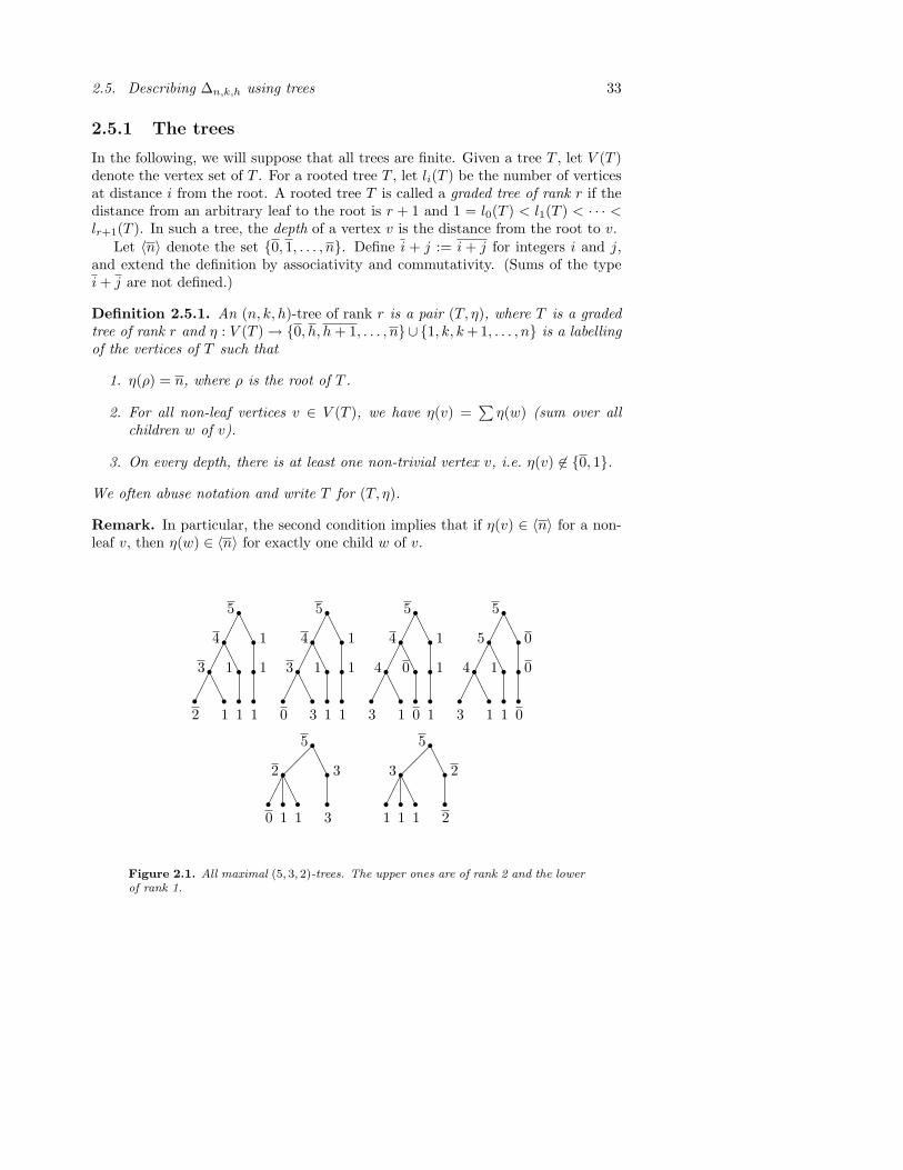
2.5. Describing ∆n,k,h using trees 33
2.5.1 The trees
In the following, we will suppose that all trees are finite. Given a tree T , let V (T )denote the vertex set of T . For a rooted tree T , let li(T ) be the number of verticesat distance i from the root. A rooted tree T is called a graded tree of rank r if thedistance from an arbitrary leaf to the root is r + 1 and 1 = l0(T ) < l1(T ) < · · · <lr+1(T ). In such a tree, the depth of a vertex v is the distance from the root to v.
Let 〈n〉 denote the set 0, 1, . . . , n. Define i + j := i + j for integers i and j,and extend the definition by associativity and commutativity. (Sums of the typei + j are not defined.)
Definition 2.5.1. An (n, k, h)-tree of rank r is a pair (T, η), where T is a gradedtree of rank r and η : V (T ) → 0, h, h + 1, . . . , n∪ 1, k, k +1, . . . , n is a labellingof the vertices of T such that
1. η(ρ) = n, where ρ is the root of T .
2. For all non-leaf vertices v ∈ V (T ), we have η(v) =∑
η(w) (sum over allchildren w of v).
3. On every depth, there is at least one non-trivial vertex v, i.e. η(v) 6∈ 0, 1.
We often abuse notation and write T for (T, η).
Remark. In particular, the second condition implies that if η(v) ∈ 〈n〉 for a non-leaf v, then η(w) ∈ 〈n〉 for exactly one child w of v.
rrr
r r rr r r r
¢¢
AA
¢¢
AA
¢¢
AA
5
4
3
2 1 1 1
1
11
rrr
r r rr r r r
¢¢
AA
¢¢
AA
¢¢
AA
5
4
3
0 3 1 1
1
11
rrr
r r rr r r r
¢¢
AA
¢¢
AA
¢¢
AA
5
4
4
3 1 0 1
1
10
rrr
r r rr r r r
¢¢
AA
¢¢
AA
¢¢
AA
5
5
4
3 1 1 0
0
01
rrr
r r r r
¡¡
AA
¢¢
AA
5
2 3
0 1 1 3
rrr
r r r r
¡¡
AA
¢¢
AA
5
3 2
1 1 1 2
Figure 2.1. All maximal (5, 3, 2)-trees. The upper ones are of rank 2 and the lowerof rank 1.
34 Paper 2. Quotient complexes and lexicographic shellability
Let T rn,k,h denote the set of (n, k, h)-trees of rank r (we will not distinguish
between isomorphic trees), and let Tn,k,h be the set of all (n, k, h)-trees so that, inparticular, Tn,k,h = ∪rT
rn,k,h.
2.5.2 The deletion operator
For an integer i, 0 < i ≤ r+1, we define the deletion operator δi : T rn,k,h → T r−1
n,k,h byδi((T, η)) := (T i, ηi), where T i is the tree obtained from T by deleting all verticesof depth i and letting the grandchildren of the depth i − 1 vertices be their newchildren. The labelling ηi is the restriction of η to V (T i). For convenience, weintroduce δi→j := δi+1 δi+2 · · · δj−1 for i < j +1. We will also use the notationδi→ := δi+1 δi+2 · · · δr+1.
2.5.3 A description of ∆n;k;h
Recall from Section 2.4 the description of the vertices of ∆n,k,h in terms of theelements of Nn,k,h. Note that each level, i.e. set of vertices of some fixed depth, ofT ∈ Tn,k,h can be viewed as an element λ ∈ Nn,k,h. The (labelled) vertices of Tcorrespond to parts in λ. A vertex v such that η(v) ∈ 〈n〉 corresponds to a nullpart. (We interpret η(v) = 0 as the non-existence of a null part.)
Let ∆rn,k,h be the set of r-dimensional simplices in ∆n,k,h. We describe a map-
ping ψ : ∆rn,k,h → T r
n,k,h as follows:Take a simplex c ∈ ∆r
n,k,h and let the chain π = πr+1 < πr · · · < π1 ⊆ Πn,k,h
be a representative of c. We construct ψ(c) level by level. The (labelled) verticesat depth i of ψ(c) are the parts in orb(πi) ∈ Nn,k,h. We put an edge between twovertices a and b, of depths i and i+1 respectively, if the block in πi+1 correspondingto b is contained in the block in πi corresponding to a. Finally, we add the rootn and put edges from it to all vertices of depth 1. It follows immediately fromthe construction that ψ is well-defined, i.e. ψ(c) does not depend on the choice ofrepresentative of c.
The following result is analogous to [57, Theorem 4.4], and the same straight-forward proof applies with obvious modifications. It allows us to use Tn,k,h as amodel of ∆n,k,h.
Proposition 2.5.2. The mapping ψ : ∆rn,k,h → T r
n,k,h is bijective. Furthermore,under ψ, inclusion in ∆n,k,h corresponds to deletion in Tn,k,h. In other words, fortwo simplices c1, c2 ∈ ∆n,k,h we have c1 ⊆ c2 iff ψ(c1) = δi1 · · · δit(ψ(c2)) forsome i1, . . . , it.
2.6 The homotopy type of ∆n,k,h
In the following we will need two projection maps µ, ν : Nn,k,h → Nn,k,h.
2.6. The homotopy type of ∆n,k,h 35
Definition 2.6.1. Let λ ∈ Nn,k,h be given. Recall that null(λ) is the size of thenull part of λ.
1. Define µ(λ) to be the maximal element µ ≤ λ such that null(µ) = 0 and allnon-singleton parts of µ have size k.
2. Define ν(λ) to be the maximal element ν ≤ λ such that null(ν) = null(λ) andall non-singleton non-null parts of ν have size k.
3. We say that λ is µ-like (ν-like) if λ is fixed by µ (ν).
For example, with n = 7 and k = 2, µ(3, 3, 1) = 2, 2, 1, 1, 1, which is a µ-likepartition, and ν(3, 3, 1) = 3, 2, 1, 1, which is ν-like.
Note that λ ∈ Nn,k,h is µ-like iff null(λ) = 0 and all non-singleton parts of λhave size k. Similarly, λ is ν-like iff all non-singleton non-null parts of λ have sizek.
2.6.1 The Dn;k case
Theorem 2.6.2. The complex ∆n,k,k is collapsible.
Proof. The idea is the same as in Kozlov’s proof of [56, Theorem 4.1]. We will givean acyclic matching on the face poset P (∆n,k,k). In view of Proposition 2.5.2, wewill consider the elements of P (∆n,k,k) to be (n, k, k)-trees. Recall from Section2.5.3 that the levels of a tree T ∈ P (∆n,k,k) are viewed as elements of Nn,k,k. Letλi(T ) ∈ Nn,k,k denote the element obtained from depth i in T .
P (∆n,k,k) is partitioned into the sets X, Y and Z in the following way. Pick atree T ∈ P (∆n,k,k). If λi(T ) is µ-like for all i, then T belongs to Z. Otherwise, leti be the largest index such that λi(T ) is not µ-like. If µ(λi(T )) = λi+1(T ), then Tbelongs to X. If, on the other hand, µ(λi(T )) 6= λi+1(T ), then T belongs to Y .
Let T ∈ Y be given, and let i be the largest index such that λi(T ) is not µ-like.It is easily seen that there is a unique way (up to tree-isomorphisms) to insert anew level corresponding to µ(λi(T )) directly beneath level i in T . The tree T thusobtained covers T (since δi+1(T ) = T ) and belongs to X. Conversely, given T ∈ X,we construct T ∈ Y uniquely by deleting the level below the deepest not µ-like levelin T . Hence we have a bijection ˜ : Y → X such that T covers T .
It remains to show that our matching is acyclic. To this end, suppose T1, T2 ∈ Y ,T1 6= T2 and that T1 covers T2. Since T2 6= T1, T2 must be obtained from T1 bydeleting some other level than the one below the deepest not µ-like level. This otherlevel must in fact be the deepest not µ-like level; otherwise we would have T2 ∈ X.Hence the number of µ-like levels in T2 is one larger than in T1. Repeating thisargument shows the non-existence of a sequence T1, . . . , Tt ∈ Y such that T1 = Tt,Ti 6= Ti+1 and Ti covers Ti+1 for i ∈ [t− 1]. Hence the matching is acyclic.
Since the property that all levels are µ-like is preserved under deletion of levels,Z is a subcomplex of ∆n,k,k. Theorem 2.2.2 shows that there is a sequence ofelementary collapses transforming ∆n,k,k to Z. This subcomplex consists of the
36 Paper 2. Quotient complexes and lexicographic shellability
(n, k, k)-trees in which every level is µ-like. There is obviously exactly one maximalsuch tree. Hence, the subcomplex given by Z is a simplicial complex generated byone simplex and thus collapsible.
2.6.2 The Bn;k;h case
When h < k, the proof of Theorem 2.6.2 fails. The reason is that for h ≤ i < k, wehave µ(i, 1, 1, . . . , 1) = 1, 1, . . . , 1 which is not in the proper part of Nn,k,h. Toovercome this, we will use ν instead of µ. As before, we will use simplices of ∆n,k,h
and their tree representations interchangeably.
Definition 2.6.3. Let Un,k,h be the subcomplex of ∆n,k,h consisting of the (n, k, h)-trees in which every level is ν-like.
Lemma 2.6.4. The complexes ∆n,k,h and Un,k,h are homotopy equivalent.
Proof. Except for the last two sentences, the proof of Theorem 2.6.2 goes throughwith obvious modifications if we replace µ with ν.
Theorem 2.6.5. Let h < k. If n ≡ 0 (mod k), then ∆n,k,h is homotopy equivalentto a sphere of dimension 2n
k − 2. If n ≡ h (mod k), then ∆n,k,h is homotopyequivalent to a sphere of dimension 2n−h
k − 1. Otherwise, ∆n,k,h is contractible.
Proof. In the light of Lemma 2.6.4, we restrict our attention to Un,k,h. We let P bethe set of ν-like elements in Nn,k,h and we choose to order them in reverse fashion toNn,k,h. That is, κ ≤P λ if λ refines κ as number partitions and null(λ) ≤ null(κ).The map f : vert(Un,k,h) → [dim(Un,k,h)+1], where f(v) is the maximal cardinalityof a P -chain with v as largest element clearly balances Un,k,h. We identify 0 = nand 1 = 1, 1, . . . , 1 in Un,k,h.
We give a chain-labelling of Un,k,h which induces a CL-shelling. Our poset oflabels is Λ = A < B < C1 < · · · < Cn−1 < D. The label of a root simplex cin Un,k,h is determined by the refinement taking place between level r = rank(Tc)and the leaves of its corresponding tree Tc = ψ(c \ 0). (If c contains 1, and henceis a facet, we let Tc be the tree ψ(c \ 0, 1) to which we have attached a leaf-levelcorresponding to 1 in the obvious way.) Let x = λr(Tc) and y = λr+1(Tc) (notationas in the proof of Theorem 2.6.2). Define the labelling ω : R(Un,k,h) → Λ by:
• ω(c) = A, if null(x) = null(y) + 1, i.e. if y is obtained from x by cutting asingleton off the null part.
• ω(c) = B, if h > 1, null(x) = h and null(y) = 0, i.e. if the null part in x is ofsize h and is split into singletons in y.
• ω(c) = Ci, if a non-null k-part in x is split into singletons in y and the k-partfirst appeared at depth i in Tc. By this we mean that the k-part was cut offthe null part in the refinement process between depth i− 1 and depth i in Tc.
2.6. The homotopy type of ∆n,k,h 37
• ω(c) = D, if null(x) = null(y) + k, i.e. if y is obtained from x by cutting ak-part off the null part.
Remark. If h = 1, then label B is never used. However, A plays its role in this case.
The simplices determining root intervals in Un,k,h correspond to trees which aresaturated except between some level r and the leaves. It is not hard to see, thatin every rooted interval there is a unique rising simplex and that this simplex islexicographically least on the interval. Hence, the first and second conditions ofDefinition 2.3.1 are fulfilled.
In the following, we will not make distinctions between simplices and theircorresponding trees. Let F1, . . . , Ft be the lexicographic ordering of the facets ofUn,k,h. To verify Condition 3′ of Proposition 2.3.3, pick c in Fj ∩ (∪α<jFα). Writec = δa1→b1 · · · δam→bm(Fj) for some appropriate ax, bx with ax + 2 ≤ bx andbx−1 ≤ ax. Choose Fi, i < j, such that c = δa′1→b′1 · · · δa′m→b′m(Fi) for somea′x, b′x such that a′x + 2 ≤ b′x and b′x−1 ≤ a′x. (Since Un,k,h possibly is nonpure, wedo not necessarily have ax = a′x and bx = b′x.) Suppose that Fj is rising on everyrooted interval given by δax→bx δbx→(Fj). We must show that c is contained insome simplex b ⊆ Fj ∩ (∪α<jFα) with codimFj (b) = 1.
Let a be minimal such that ω(δa→(Fj)) 6= ω(δa→(Fi)). We cannot have ax <a < bx for any x, because this would imply δax→(Fj) = δax→(Fi) and δbx→(Fj) 6=δb′x→(Fi), which is impossible since i < j and Fj is rising on the rooted intervalof δax→bx δbx→(Fj) = δax→b′x δb′x→(Fi). Thus, the refinement process whichdetermines ω(δa→(Fj)) occurs within c ⊆ Fi ∩ Fj . By the definition of ω, thisimplies ω(δa→(Fj)) = Cxj and ω(δa→(Fi)) = Cxi for some xi < xj . Moreover, weknow that ax < xi < xj < bx for some x and that ω(δxi→(Fj)) = ω(δxi+1→(Fj)) =· · · = ω(δxj→(Fj)) = D; otherwise Cxi and Cxj would correspond to differentrefinement processes within c. The label Cxj precedes Cxi in the sequence of labelsof Fj , so there is some xs such that xi ≤ xs < xs + 1 ≤ xj and Cxs+1 precedesCxs in this sequence. Now create the facet Fs which has every ω-label in commonwith Fj except that Cxs and Cxs+1 are interchanged. Then s < j and δxs(Fs) =δxs(Fj) ⊇ c. Thus c is contained in a simplex of codimension 1. Hence Un,k,h isCL-shellable.
In order to determine the homotopy type of Un,k,h, we will identify the topolog-ically falling facets in the described shelling. The homotopy type is then given byProposition 2.3.5. To this end, consider a facet F and its boundary simplex δi(F ).Let ωi and ωi+1 denote the labels of the root simplices δi→(F ) and δi+1→(F ) re-spectively. If i is a descent, i.e. ωi > ωi+1 (since Λ is a total ordering), then itis also a topological descent. Now suppose ωi ≤ ωi+1. If ωi 6= D, then no facetpreceding F contains δi(F ). This is because all labels below depth i depend onlyon refinement processes within δi(F ) in this case. The only case left to check isthus ωi = ωi+1 = D. As above, it is seen that δi(F ) is contained in some facetpreceding F if and only if the label Ci+1 precedes the label Ci, or, in other words,if the (unique) root simplex contained in F with label Ci+1 is contained in the one
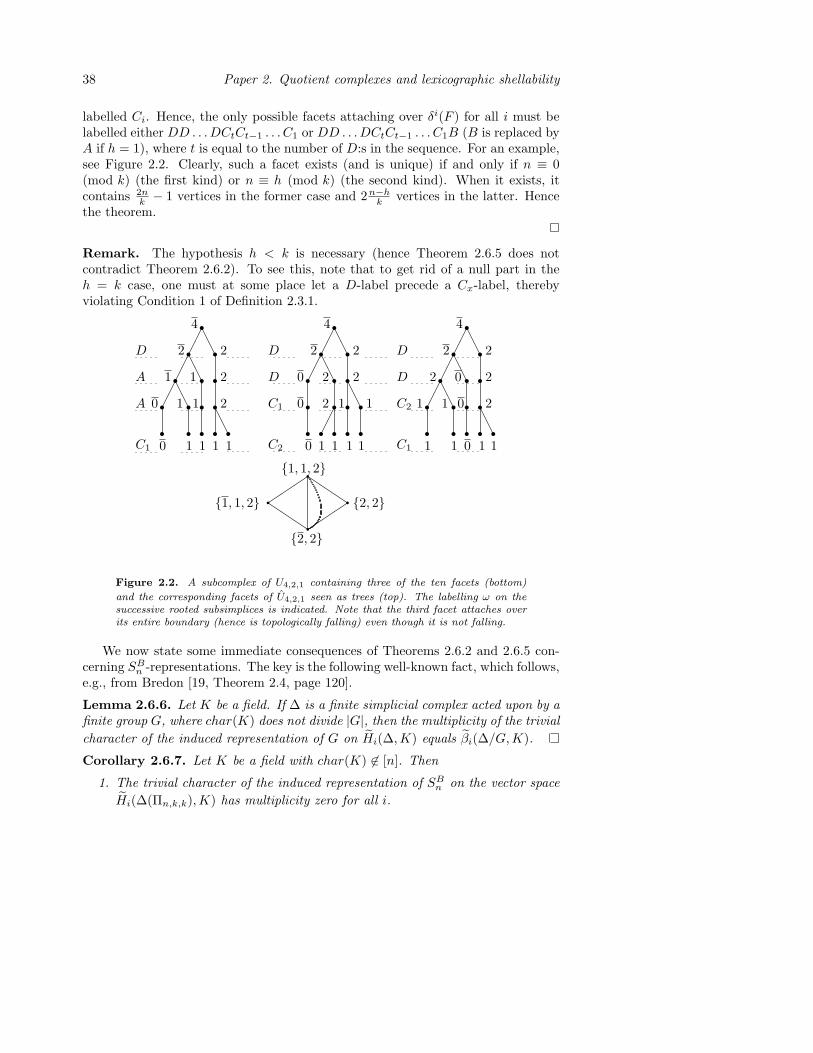
38 Paper 2. Quotient complexes and lexicographic shellability
labelled Ci. Hence, the only possible facets attaching over δi(F ) for all i must belabelled either DD . . .DCtCt−1 . . . C1 or DD . . . DCtCt−1 . . . C1B (B is replaced byA if h = 1), where t is equal to the number of D:s in the sequence. For an example,see Figure 2.2. Clearly, such a facet exists (and is unique) if and only if n ≡ 0(mod k) (the first kind) or n ≡ h (mod k) (the second kind). When it exists, itcontains 2n
k − 1 vertices in the former case and 2n−hk vertices in the latter. Hence
the theorem.
Remark. The hypothesis h < k is necessary (hence Theorem 2.6.5 does notcontradict Theorem 2.6.2). To see this, note that to get rid of a null part in theh = k case, one must at some place let a D-label precede a Cx-label, therebyviolating Condition 1 of Definition 2.3.1.
rrr
r r rr r r rr r r r r
¢¢
AA
¢¢
AA
¢¢
AA
AA
4
2 2
1 1 2
0 1 1 2
0 1 1 1 1
rrr
r r rr r r rr r r r r
¢¢
AA
¢¢
AA
AA
¢¢
4
2 2
0 2 2
0 2 1 1
0 1 1 1 1
rrr
r r rr r r rr r r r r
¢¢
AA
¢¢
AA
¢¢
AA
AA
4
2 2
2 0 2
1 1 0 2
1 1 0 1 1C1
A
A
D
C2
C1
D
D
C1
C2
D
D
´´
´Q
Q´
´´
1, 1, 2
2, 21, 1, 2
2, 2
Figure 2.2. A subcomplex of U4,2,1 containing three of the ten facets (bottom)
and the corresponding facets of U4,2,1 seen as trees (top). The labelling ω on thesuccessive rooted subsimplices is indicated. Note that the third facet attaches overits entire boundary (hence is topologically falling) even though it is not falling.
We now state some immediate consequences of Theorems 2.6.2 and 2.6.5 con-cerning SB
n -representations. The key is the following well-known fact, which follows,e.g., from Bredon [19, Theorem 2.4, page 120].
Lemma 2.6.6. Let K be a field. If ∆ is a finite simplicial complex acted upon by afinite group G, where char(K) does not divide |G|, then the multiplicity of the trivialcharacter of the induced representation of G on Hi(∆,K) equals βi(∆/G,K).
Corollary 2.6.7. Let K be a field with char(K) 6∈ [n]. Then
1. The trivial character of the induced representation of SBn on the vector space
Hi(∆(Πn,k,k),K) has multiplicity zero for all i.
2.6. The homotopy type of ∆n,k,h 39
2. Let h < k. The trivial character of the induced representation of SBn on
the vector space Hi(∆(Πn,k,h),K) has multiplicity one if n ≡ 0 (mod k) andi = 2n
k −2 or if n ≡ h (mod k) and i = 2n−hk −1. Otherwise it has multiplicity
zero.
Proof. Note that |SBn | = 2nn!. The corollary now follows from Theorem 2.6.2,
Theorem 2.6.5 and Lemma 2.6.6.

40
Paper 3.
Directed subgraph complexes
3.1 Introduction
A monotone property of a (directed or undirected) graph is one which is preservedunder deletion of edges. Hence, the set of all graphs on a particular vertex set, [n]say, that satisfy a monotone property form a simplicial complex whose vertex setis the set of edges of the graphs. In numerous recent papers, see e.g. [2, 18, 24,53, 55, 74, 75], the topological properties of such complexes of graphs have beenstudied. Although most papers have dealt with complexes of all graphs having aparticular property P , it is indeed natural to study the complex of all subgraphsof a given graph that satisfy P . The purpose of this paper is to study directedgraph complexes of this type. The properties that we focus on are acyclicity andstrong non-connectivity. Both were studied by Bjorner and Welker [18] in thecase of all graphs. We adapt their techniques in order to generalize their results.We also consider some consequences related to topics such as finite topologies andhyperplane arrangements.
In Section 3.3 we study acyclic graphs. The homotopy type of the complex ofacyclic subgraphs of any given directed graph is determined. It is either a homo-topy sphere or contractible. Thereafter, in Section 3.4, we focus on not stronglyconnected graphs. More precisely, we compute the homotopy type of the complexof not strongly connected subgraphs of a directed graph, if the graph belongs to aparticular class, which we call 2-dense graphs.
We begin, however, with a brief survey in the next section of the more or lessstandard tools from topological combinatorics that will be made use of later.Acknowledgement. The author is grateful to his advisor Anders Bjorner forsuggesting the study of subgraph complexes.
41
42 Paper 3. Directed subgraph complexes
3.2 Basic topological combinatorics
Here, we briefly review the parts of the topological combinatorics machinery thatwe will use later. For more details we refer to the survey [10].
To any poset P , we associate the order complex ∆(P ). It is the simplicialcomplex whose faces are the chains of P . Similarly, to any simplicial complex Σ,we associate its face poset P (Σ) which consists of the nonempty faces of Σ orderedby inclusion. The complex ∆(P (Σ)) is the barycentric subdivision of Σ, hence it ishomeomorphic to Σ. (We do not distinguish notationally between a complex andits underlying topological space.)
Our first two tools are due to Quillen [63]. In a poset P with an element x ∈ P ,we write P≤x = y ∈ P | y ≤ x.Lemma 3.2.1 (Quillen Fiber Lemma). Let P and Q be posets, and suppose wehave an order-preserving map f : P → Q such that ∆(f−1(Q≤q)) is contractiblefor all q ∈ Q. Then ∆(P ) is homotopy equivalent to ∆(Q).
Lemma 3.2.2 (Closure Lemma). Let P be a poset, and suppose that f : P → Pis a closure operator (i.e. f(p) ≥ p and f2(p) = f(p) for all p ∈ P ). Then ∆(P ) ishomotopy equivalent to ∆(f(P )).
If a poset P has unique minimal and maximal elements, denoted by 0 and 1,respectively, then its proper part is P = P \ 0, 1.
The next result can be found e.g. in [10].
Lemma 3.2.3. Let L be a lattice. Form a simplicial complex Σ whose faces arethose subsets of the atoms of L whose joins are not the top element. Then ∆(L)and Σ are homotopy equivalent.
For simplicial complexes ∆1 and ∆2, let ∆1∗∆2 denote their join. The followinglemma is well-known.
Lemma 3.2.4. Suppose ∆i is homotopy equivalent to a wedge of ni spheres ofdimension di, i = 1, 2. Then ∆1 ∗ ∆2 is homotopy equivalent to a wedge of n1n2
spheres of dimension d1 + d2 + 1.
Finally, we need a convenient collapsibility lemma stated by Bjorner and Welker[18]. For a simplicial complex ∆ on the vertex set [n], a face F ∈ ∆ and a vertexi ∈ [n], define a map ∆ → ∆ by
F 7→ F ± i =
F ∪ i if i 6∈ F ,F \ i if i ∈ F .
Lemma 3.2.5. If ∆1 ⊆ ∆2 are simplicial complexes on the vertex set [n] and thereexist vertices i, j ∈ [n] such that F ± i maps ∆2 \∆1 to itself and F ± j maps ∆1
to itself, then ∆2 is contractible (and so is ∆1).
3.3. Acyclic subgraphs 43
3.3 Acyclic subgraphs
From now on, let G be a fixed directed graph on vertex set [n]. Like all graphs inthis paper (directed and undirected), G will be assumed to have no loops or multipleedges. Our first object of study is the complex ∆ACY
G of all acyclic subgraphs ofG. More precisely, with E(G) denoting the edge set of G, we define
∆ACYG = F ⊆ E(G) | ([n], F ) has no directed cycle.
Let Tr(·) denote transitive closure. Define PosG to be the following subset of allpartial orders on [n]: a poset belongs to PosG iff its comparability graph is Tr(H)for some subgraph H of G. Under inclusion, PosG is a poset. We denote its uniqueminimal element, the empty relation, by 0. In the following lemma, the case of Gbeing the complete graph is [18, Lemma 2.1].
Lemma 3.3.1. The complexes ∆(PosG \0) and ∆ACYG are homotopy equivalent.
Proof. The map H 7→ Tr(H)∩G is a closure operator on P (∆ACYG ). We claim that
its image is isomorphic to PosG \ 0. To show this, it suffices to check that Tr(H)can be reconstructed from Tr(H)∩G; it can, since Tr(H) = Tr(Tr(H)∩(G)). Thus,by Lemma 3.2.2, the barycentric subdivision of ∆ACY
G is homotopy equivalent to∆(PosG \ 0).
Recall that the vertices of any directed graph can be partitioned into stronglyconnected components: x and y belong to the same component iff there exist directedpaths from x to y and from y to x. If every vertex belongs to the same component,then the graph is strongly connected.
Bjorner and Welker stated the following theorem in the case of G being thecomplete graph only. However, it is straightforward to check that their proof goesthrough in the more general case, too.
Theorem 3.3.2 (See Theorem 2.2 in [18]). If G is strongly connected, then∆(PosG \ 0) is homotopy equivalent to the (n− 2)-sphere.
It is now straightforward to prove the main result of this section.
Theorem 3.3.3. If G is a disjoint union of k strongly connected components,then ∆ACY
G is homotopy equivalent to the (n− 1− k)-sphere. Otherwise, ∆ACYG is
contractible.
Proof. If G is not a disjoint union of strongly connected components, then G hasan edge e which is not included in any cycle. Thus, ∆ACY
G is a cone with apex e.Now suppose that G is a disjoint union of k strongly connected components. If
k = 1, then we are done by Theorem 3.3.2 and Lemma 3.3.1. Otherwise, ∆ACYG is a
44 Paper 3. Directed subgraph complexes
join of k complexes of this type. Applying Lemma 3.2.4 (k− 1) times, we concludethat ∆ACY
G is homotopy equivalent to the sphere of dimension
k∑
i=1
(ai − 2) + k − 1 = n− k − 1,
where ai is the number of vertices in the ith component of G.
Recall that a quasiorder is a reflexive and transitive relation. The poset (actuallya lattice) of quasiorders on [n] is a well-studied object (see e.g. [33]), mainly sincequasiorders on [n] correspond in a 1-1 fashion to topologies on [n]. The subposetPosn of partial orders on [n] then corresponds to the topologies that satisfy the T0
separation axiom. Thus, the next corollary can be thought of as a statement aboutfinite topologies.
For a quasiorder R on [n], let PosRn be the poset of all posets that are contained
in R.
Corollary 3.3.4. Let R be a quasiorder on [n]. If R is in fact an equivalencerelation with k equivalence classes, then ∆(PosR
n \ 0) is homotopy equivalent tothe (n− 1− k)-sphere. Otherwise, ∆(PosR
n \ 0) is contractible.
Proof. There is an obvious correspondence between quasiorders and transitivelyclosed directed graphs. Applying Theorem 3.3.3 with the graph corresponding toR yields the result via Lemma 3.3.1.
3.4 Not strongly connected subgraphs
In this section we turn our attention to ∆NSCG , the complex of subgraphs of G that
are not strongly connected. More precisely,
∆NSCG = F ⊆ E(G) | ([n], F ) is not strongly connected.
Again, the case of G being the complete graph was analysed in [18].Let ΠG be the subposet of the partition lattice Πn consisting of the possible
partitions into strongly connected components of subgraphs of G. The partitioncorresponding to a graph H is denoted by π(H). Clearly, if π(H), π(H ′) ∈ ΠG, thentheir join (in Πn) belongs to ΠG. Since 0 ∈ ΠG, we conclude that ΠG is a lattice,although it is easy to construct an example showing that ΠG is not a sublattice ofΠn.
By a minimal cyclic set of G, we mean an inclusion-minimal subset S ⊆ [n]with the property that some directed G-cycle has S as vertex set. Clearly, suchsets correspond to atoms of ΠG. We let G denote the hypergraph on [n] whoseedges are precisely the minimal cyclic sets of G.
Directed graphs whose minimal cyclic sets all have cardinality two will be im-portant to us. We call such graphs 2-dense. Thus, G is 2-dense iff every cycle
3.4. Not strongly connected subgraphs 45
contains two vertices that themselves form a cycle in G, i.e. iff G is an ordinarygraph.
Recall that to any (undirected) graph H = ([n], E), one associates the graphicalarrangement AH . This is a hyperplane arrangement in Rn containing |E| differenthyperplanes, each given by a coordinate equation xi = xj for i, j ∈ E. Itsintersection lattice, L(AH), is the lattice of all possible intersections of collectionsof such hyperplanes, ordered by reverse inclusion.
Theorem 3.4.1. Suppose that G is 2-dense. If G is connected, the order complexes∆(ΠG) and ∆(L(A bG)) are homotopy equivalent. If G is disconnected, then ∆(ΠG)is contractible.
Proof. Suppose that G is 2-dense and denote the edge set of G by E(G). Let Σdenote the simplicial complex on the vertex set E(G) whose simplices are given bythe disconnected subgraphs of G. By Lemma 3.2.3, we have ∆(ΠG) ' Σ.
If G is disconnected, then Σ is just a simplex, and therefore contractible.Now suppose that G is connected. Taking transitive closure and then intersect-
ing with G yields a closure operator on P (Σ). Its image is isomorphic to the posetof all partitions of [n] that arise as sets of connected components in nonempty dis-connected subgraphs of G. Clearly, this poset is isomorphic to L(A bG). By Lemma3.2.2, the theorem follows.
Remark. Requiring G to be 2-dense is not necessary in the above theorem. If Gis not 2-dense, then A bG should be interpreted as the hypergraph subspace arrange-ment given by G. This generalization will not, however, be useful to us later inthis paper. For more on hypergraph arrangements and subspace arrangements ingeneral, we refer to the survey [9].
Bjorner’s and Welker’s proof of [18, Lemma 3.1] goes through to prove themore general statement below. We state it here to be able to point out where the2-density assumption is being used. Below, P ⊕Q denotes ordinal sum of posets.
Lemma 3.4.2 (See Lemma 3.1 in [18]). If G is 2-dense, then ∆NSCG and
∆(PosG \ 0 ⊕ΠG) are homotopy equivalent.
Proof. For convenience, let Q = PosG \ 0 ⊕ ΠG. Consider the natural order-preserving surjection ϕ : P (∆NSC
G ) → Q given by
ϕ(H) =
Tr(H) ∈ PosG \ 0 if H is acyclic,π(H) ∈ ΠG otherwise.
In order to use Lemma 3.2.1, we study the inverse images of ϕ.To begin with, we pick p ∈ PosG\0. Clearly, ϕ−1(Q≤p) has a unique maximal
element, namely the intersection of G and (the comparability graph of) p. Thiselement is a cone point, and ∆(ϕ−1(Q≤p)) is contractible.
46 Paper 3. Directed subgraph complexes
Now choose τ ∈ ΠG. Since G is 2-dense, any non-singleton block of τ containsa directed G-cycle of length two. Without loss of generality, suppose that 1 and 2form such a cycle. Let ∆2 = ∆(ϕ−1(Q≤τ )) and let ∆1 ⊆ ∆2 be the subcomplexcomprising the graphs that contain no directed path from 1 to 2 except possiblythe edge (1, 2). Now observe that adding the edge (2, 1) to H ∈ ∆1 affects thepartition into strongly connected components at worst by merging the part whichcontains 1 with that which contains 2. This shows that H 7→ H ± (2, 1) maps ∆1
into itself. Similarly, H 7→ H ± (1, 2) maps ∆2 \∆1 into itself. Thus, by Lemma3.2.5, ∆(ϕ−1(Q≤τ )) is contractible, and we are done.
Using χ bG(t) to denote the chromatic polynomial of G, we are now in positionto state the main theorem. Note that the case of G being not strongly connectedis uninteresting since ∆NSC
G is just a simplex in this case.
Theorem 3.4.3. If G is 2-dense and strongly connected, then ∆NSCG is homotopy
equivalent to a wedge of (2n − 4)-dimensional spheres. The number of spheres is|χ′bG(0)|.
Proof. By Lemma 3.4.2 and the definition of ordinal sums, ∆NSCG ' ∆(PosG\0)∗
∆(ΠG).If G is disconnected, ∆NSC
G is contractible by Theorem 3.4.1. In this case, thelinear term of χ bG(t), and thus its absolute value |χ′bG(0)|, vanishes as desired. We
may therefore assume that G is connected.It is well-known, see e.g. Rota [65], that the characteristic polynomial of L(A bG)
and the chromatic polynomial of G coincide, i.e.
χ bG(t) =∑
x∈L(A bG)
µ(0, x)tdim(x),
where µ is the Mobius function of L(A bG). Moreover, by a theorem of Bjorner[6], ∆(L(A bG)) has the homotopy type of a wedge of |µ(0, 1)| spheres of dimensioncodim(1) − 2. Since the top element has dimension one in our case, we concludethat ∆(L(A bG)), and therefore ∆(ΠG), has the homotopy type of a wedge of (n−3)-dimensional spheres and that the number of spheres is the absolute value of thelinear term of χ bG(t).
Theorem 3.3.3 shows that ∆(PosG \ 0) ' Sn−2, so, by Lemma 3.2.4, we aredone.
Remark. The number of spheres above, i.e. the absolute value of the linear termof the chromatic polynomial of G, has a nice interpretation due to Greene andZaslavsky [40]. It is the number of acyclic orientations of G having a unique fixedsink. See also [37].
3.4. Not strongly connected subgraphs 47
Corollary 3.4.4 (Theorem 1.2 in [18]). The complex of all not strongly con-nected directed graphs on [n] is homotopy equivalent to a wedge of (n− 1)! spheresof dimension 2n− 4.
Proof. If G is the complete directed graph, then G is the complete undirected graph.The linear term in its chromatic polynomial is (−1)n−1(n− 1)!.

48

Part II
Bruhat intervals
49

50
Paper 4.
Bruhat intervals of length 4in Weyl groups
4.1 Introduction
The Bruhat ordering of Coxeter groups appears in a wide variety of mathematicalcontexts. As an example (perhaps the most prominent), suppose that G is a simplyconnected semisimple algebraic group over an algebraically closed field with Borelsubgroup B. Then the incidences between the closed Schubert cells in the Bruhatdecomposition of the flag variety G/B are governed by the Bruhat order on thecorresponding Weyl group.
Answering a question of Bjorner [7], Dyer [28] showed that (up to isomorphism)only finitely many posets of each length n occur as intervals in the Bruhat orderon finite Coxeter groups. It is natural to ask which posets. Work of Bjorner andWachs [15] yields as a byproduct the solution for n = 2, 3.
In this paper we solve the classification problem when n = 4 for Weyl groups(i.e. finite Coxeter groups whose Coxeter graphs contain only labels from 2, 3, 4, 6)and for the smaller classes of simply-laced Weyl groups (with labels from 2, 3)and symmetric groups.
Our strategy is as follows. Relying on the results in [28], we need only inspecta small number (four) of particular Weyl groups. Using a computer, it is possibleto single out all occurring isomorphism types in these groups by brute force; wereport on such a search at the end of the paper. Most of the paper, however, isoccupied by another approach, which we now describe. To each interval a so-calledcrown index is associated. Basically, it records some of the valencies in the Hassediagram. Thus, it is much easier to compute than the entire isomorphism type ofthe interval. Aided by computer, we list all crown indices that occur in the fourgroups. Using the interpretation of Bruhat intervals as regular cell decompositions
51
52 Paper 4. Bruhat intervals of length 4 in Weyl groups
of spheres given in [8] and the bearing of the crown index on this decomposition,we determine which isomorphism types occur within each crown index class.
Why not just be satisfied with the first method and leave all work to the com-puter? There are several reasons. First of all, there is always some uncertaintyassociated with computer-based proofs. For instance, are there bugs? Althoughour methods both rely on extensive computer calculations, they are independentof each other. Their agreement vastly diminishes the probability of error. Anotherreason is that the second method provides combinatorial insight. Structural state-ments such as Lemmata 4.3.3 and 4.3.4, Proposition 4.3.5 and the proof of Theorem4.3.6 explain some of what is going on from a theoretical viewpoint. Also, the crownindex approach may conceivably be possible to generalize to larger Bruhat intervals.
The rest of the paper is organized in the following way. We begin with a briefreview of some important properties of the Bruhat order and the aforementionedresults of Bjorner and Wachs and Dyer. Then, in Section 4.3, we perform the actualclassification. The crown indices are defined and calculated in the first subsection.In the second subsection, the connection between Bruhat intervals of length 4, theirinterpretation as cell complexes and their crown index is stated to pave the wayfor the main theorem in the third subsection. Finally, in Section 4.4, we present abrute force computer calculation in agreement with the previous results.
Acknowledgement. The author would like to thank his advisor Anders Bjornerfor the numerous suggestions that have aided and improved this work. An anony-mous referee has also been very helpful.
4.2 Foundations
We will assume familiarity with basic Coxeter group theory. See e.g. Humphreys [50]for anything not explained here. We will also use basic notions from combinatorialtopology regarding regular CW complexes and their face posets. We refer the readerto Bjorner [10] for details.
Throughout the paper, (W,S) will be a Coxeter system. Denote its set ofreflections by T and let ` : W → N be the length function.
Definition 4.2.1. The Bruhat order on W , denoted Br(W ), is the poset (W,≤),where ≤ is defined by:
w ≤ w′ iff there exist t1, . . . , ti ∈ T such that w′ = wt1 . . . ti
and `(wt1 . . . tj−1) < `(wt1 . . . tj) for all j ≤ i.
Although not obvious from the definition, it is a fact that Br(W ) is a rankedposet with ` as rank function. Important to us is that the operation of takingdirect products carries over from Coxeter groups to Bruhat order, i.e. Br(W×W ′) ∼=Br(W )×Br(W ′). This reduces the interval classification problem to one concerningirreducible groups only. Another important property is that if W is finite, then
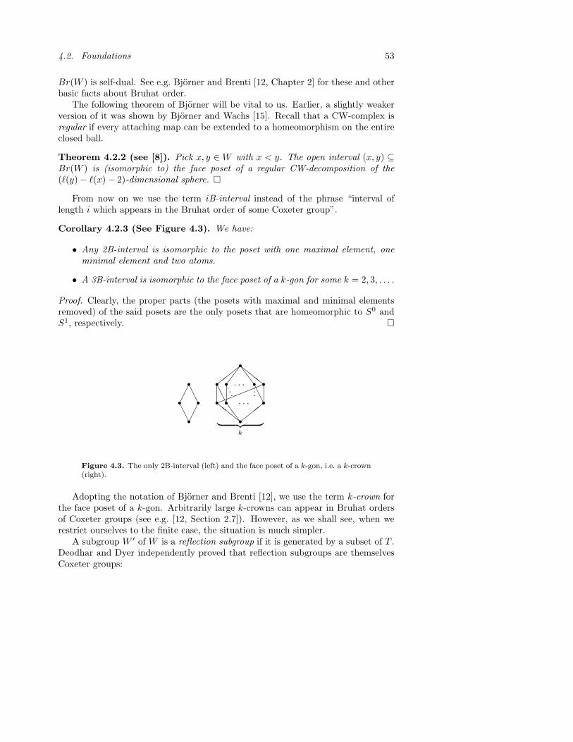
4.2. Foundations 53
Br(W ) is self-dual. See e.g. Bjorner and Brenti [12, Chapter 2] for these and otherbasic facts about Bruhat order.
The following theorem of Bjorner will be vital to us. Earlier, a slightly weakerversion of it was shown by Bjorner and Wachs [15]. Recall that a CW-complex isregular if every attaching map can be extended to a homeomorphism on the entireclosed ball.
Theorem 4.2.2 (see [8]). Pick x, y ∈ W with x < y. The open interval (x, y) ⊆Br(W ) is (isomorphic to) the face poset of a regular CW-decomposition of the(`(y)− `(x)− 2)-dimensional sphere. ¤
From now on we use the term iB-interval instead of the phrase “interval oflength i which appears in the Bruhat order of some Coxeter group”.
Corollary 4.2.3 (See Figure 4.3). We have:
• Any 2B-interval is isomorphic to the poset with one maximal element, oneminimal element and two atoms.
• A 3B-interval is isomorphic to the face poset of a k-gon for some k = 2, 3, . . . .
Proof. Clearly, the proper parts (the posets with maximal and minimal elementsremoved) of the said posets are the only posets that are homeomorphic to S0 andS1, respectively.
rr r
rAA
¢¢
¢¢
AA
r r r rr r r
r
rccc
SS
###
###
¶¶
ccc
SS
AA
AA!!!!!p p p ppp
. . .
. . .
︸ ︷︷ ︸k
Figure 4.3. The only 2B-interval (left) and the face poset of a k-gon, i.e. a k-crown(right).
Adopting the notation of Bjorner and Brenti [12], we use the term k-crown forthe face poset of a k-gon. Arbitrarily large k-crowns can appear in Bruhat ordersof Coxeter groups (see e.g. [12, Section 2.7]). However, as we shall see, when werestrict ourselves to the finite case, the situation is much simpler.
A subgroup W ′ of W is a reflection subgroup if it is generated by a subset of T .Deodhar and Dyer independently proved that reflection subgroups are themselvesCoxeter groups:
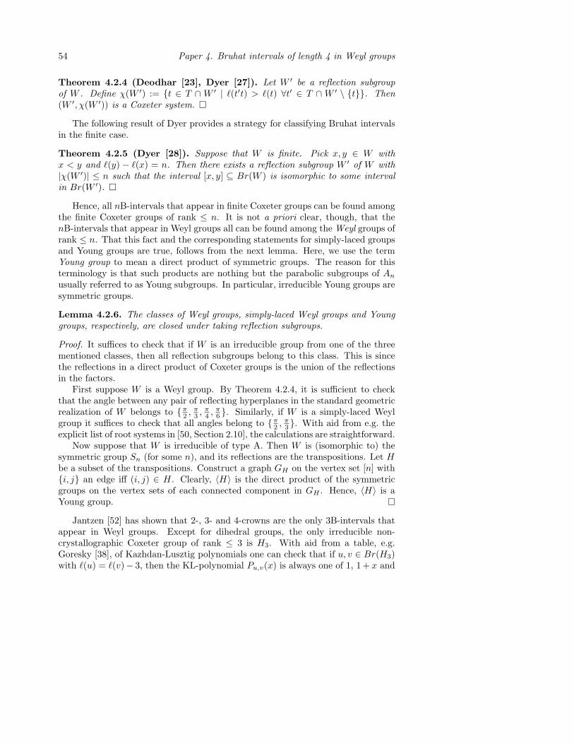
54 Paper 4. Bruhat intervals of length 4 in Weyl groups
Theorem 4.2.4 (Deodhar [23], Dyer [27]). Let W ′ be a reflection subgroupof W . Define χ(W ′) := t ∈ T ∩ W ′ | `(t′t) > `(t) ∀t′ ∈ T ∩ W ′ \ t. Then(W ′, χ(W ′)) is a Coxeter system. ¤
The following result of Dyer provides a strategy for classifying Bruhat intervalsin the finite case.
Theorem 4.2.5 (Dyer [28]). Suppose that W is finite. Pick x, y ∈ W withx < y and `(y) − `(x) = n. Then there exists a reflection subgroup W ′ of W with|χ(W ′)| ≤ n such that the interval [x, y] ⊆ Br(W ) is isomorphic to some intervalin Br(W ′). ¤
Hence, all nB-intervals that appear in finite Coxeter groups can be found amongthe finite Coxeter groups of rank ≤ n. It is not a priori clear, though, that thenB-intervals that appear in Weyl groups all can be found among the Weyl groups ofrank ≤ n. That this fact and the corresponding statements for simply-laced groupsand Young groups are true, follows from the next lemma. Here, we use the termYoung group to mean a direct product of symmetric groups. The reason for thisterminology is that such products are nothing but the parabolic subgroups of An
usually referred to as Young subgroups. In particular, irreducible Young groups aresymmetric groups.
Lemma 4.2.6. The classes of Weyl groups, simply-laced Weyl groups and Younggroups, respectively, are closed under taking reflection subgroups.
Proof. It suffices to check that if W is an irreducible group from one of the threementioned classes, then all reflection subgroups belong to this class. This is sincethe reflections in a direct product of Coxeter groups is the union of the reflectionsin the factors.
First suppose W is a Weyl group. By Theorem 4.2.4, it is sufficient to checkthat the angle between any pair of reflecting hyperplanes in the standard geometricrealization of W belongs to π
2 , π3 , π
4 , π6 . Similarly, if W is a simply-laced Weyl
group it suffices to check that all angles belong to π2 , π
3 . With aid from e.g. theexplicit list of root systems in [50, Section 2.10], the calculations are straightforward.
Now suppose that W is irreducible of type A. Then W is (isomorphic to) thesymmetric group Sn (for some n), and its reflections are the transpositions. Let Hbe a subset of the transpositions. Construct a graph GH on the vertex set [n] withi, j an edge iff (i, j) ∈ H. Clearly, 〈H〉 is the direct product of the symmetricgroups on the vertex sets of each connected component in GH . Hence, 〈H〉 is aYoung group.
Jantzen [52] has shown that 2-, 3- and 4-crowns are the only 3B-intervals thatappear in Weyl groups. Except for dihedral groups, the only irreducible non-crystallographic Coxeter group of rank ≤ 3 is H3. With aid from a table, e.g.Goresky [38], of Kazhdan-Lusztig polynomials one can check that if u, v ∈ Br(H3)with `(u) = `(v)− 3, then the KL-polynomial Pu,v(x) is always one of 1, 1 + x and
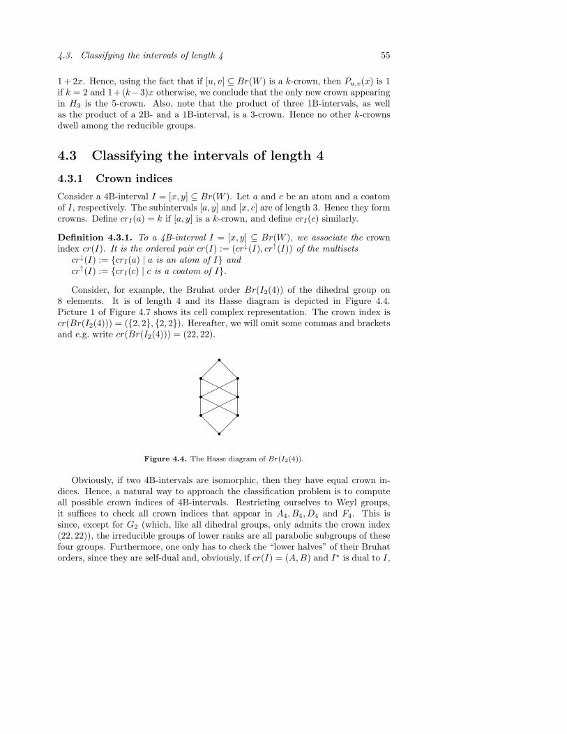
4.3. Classifying the intervals of length 4 55
1 + 2x. Hence, using the fact that if [u, v] ⊆ Br(W ) is a k-crown, then Pu,v(x) is 1if k = 2 and 1+(k−3)x otherwise, we conclude that the only new crown appearingin H3 is the 5-crown. Also, note that the product of three 1B-intervals, as wellas the product of a 2B- and a 1B-interval, is a 3-crown. Hence no other k-crownsdwell among the reducible groups.
4.3 Classifying the intervals of length 4
4.3.1 Crown indices
Consider a 4B-interval I = [x, y] ⊆ Br(W ). Let a and c be an atom and a coatomof I, respectively. The subintervals [a, y] and [x, c] are of length 3. Hence they formcrowns. Define crI(a) = k if [a, y] is a k-crown, and define crI(c) similarly.
Definition 4.3.1. To a 4B-interval I = [x, y] ⊆ Br(W ), we associate the crownindex cr(I). It is the ordered pair cr(I) := (cr↓(I), cr↑(I)) of the multisets
cr↓(I) := crI(a) | a is an atom of I andcr↑(I) := crI(c) | c is a coatom of I.Consider, for example, the Bruhat order Br(I2(4)) of the dihedral group on
8 elements. It is of length 4 and its Hasse diagram is depicted in Figure 4.4.Picture 1 of Figure 4.7 shows its cell complex representation. The crown index iscr(Br(I2(4))) = (2, 2, 2, 2). Hereafter, we will omit some commas and bracketsand e.g. write cr(Br(I2(4))) = (22, 22).
rr rr rr r
r
@@
¡¡
©©©©
HHHH HHHH
©©©©¡¡
@@
Figure 4.4. The Hasse diagram of Br(I2(4)).
Obviously, if two 4B-intervals are isomorphic, then they have equal crown in-dices. Hence, a natural way to approach the classification problem is to computeall possible crown indices of 4B-intervals. Restricting ourselves to Weyl groups,it suffices to check all crown indices that appear in A4, B4, D4 and F4. This issince, except for G2 (which, like all dihedral groups, only admits the crown index(22, 22)), the irreducible groups of lower ranks are all parabolic subgroups of thesefour groups. Furthermore, one only has to check the “lower halves” of their Bruhatorders, since they are self-dual and, obviously, if cr(I) = (A, B) and I? is dual to I,
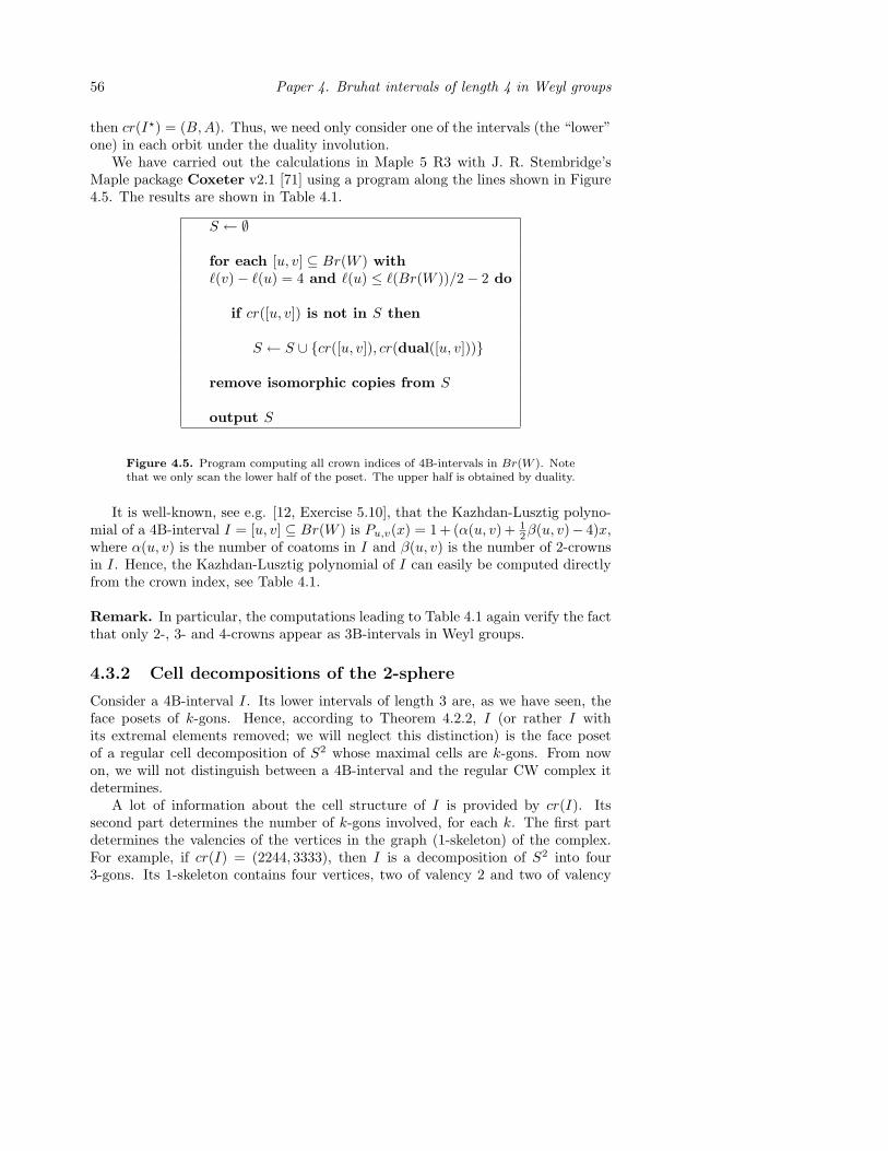
56 Paper 4. Bruhat intervals of length 4 in Weyl groups
then cr(I?) = (B, A). Thus, we need only consider one of the intervals (the “lower”one) in each orbit under the duality involution.
We have carried out the calculations in Maple 5 R3 with J. R. Stembridge’sMaple package Coxeter v2.1 [71] using a program along the lines shown in Figure4.5. The results are shown in Table 4.1.
S ← ∅
for each [u, v] ⊆ Br(W ) with`(v)− `(u) = 4 and `(u) ≤ `(Br(W ))/2− 2 do
if cr([u, v]) is not in S then
S ← S ∪ cr([u, v]), cr(dual([u, v]))
remove isomorphic copies from S
output S
Figure 4.5. Program computing all crown indices of 4B-intervals in Br(W ). Notethat we only scan the lower half of the poset. The upper half is obtained by duality.
It is well-known, see e.g. [12, Exercise 5.10], that the Kazhdan-Lusztig polyno-mial of a 4B-interval I = [u, v] ⊆ Br(W ) is Pu,v(x) = 1 + (α(u, v) + 1
2β(u, v)− 4)x,where α(u, v) is the number of coatoms in I and β(u, v) is the number of 2-crownsin I. Hence, the Kazhdan-Lusztig polynomial of I can easily be computed directlyfrom the crown index, see Table 4.1.
Remark. In particular, the computations leading to Table 4.1 again verify the factthat only 2-, 3- and 4-crowns appear as 3B-intervals in Weyl groups.
4.3.2 Cell decompositions of the 2-sphere
Consider a 4B-interval I. Its lower intervals of length 3 are, as we have seen, theface posets of k-gons. Hence, according to Theorem 4.2.2, I (or rather I withits extremal elements removed; we will neglect this distinction) is the face posetof a regular cell decomposition of S2 whose maximal cells are k-gons. From nowon, we will not distinguish between a 4B-interval and the regular CW complex itdetermines.
A lot of information about the cell structure of I is provided by cr(I). Itssecond part determines the number of k-gons involved, for each k. The first partdetermines the valencies of the vertices in the graph (1-skeleton) of the complex.For example, if cr(I) = (2244, 3333), then I is a decomposition of S2 into four3-gons. Its 1-skeleton contains four vertices, two of valency 2 and two of valency

4.3. Classifying the intervals of length 4 57
# crown index K-L A4 B4 D4 F4
1. (22, 22) 1 -√
-√
2. (233, 233) 1√ √ √ √
3. (334, 2233) 1 + x√ √ √ √
4. (2233, 334) 1√ √ √ √
5. (2334, 2334) 1 + x -√
-√
6. (3333, 2244) 1 + x -√
-√
7. (2244, 3333) 1 + x -√
-√
8. (3333, 3333) 1√ √ √ √
9. (33334, 33334) 1 + x√ √ √ √
10. (333333, 33444) 1 + x√ √ √ √
11. (33444, 333333) 1 + 2x√ √ √ √
12. (333344, 333344) 1 + 2x -√
-√
13. (334444, 3333334) 1 + 3x -√
-√
14. (3333334, 334444) 1 + 2x -√
-√
15. (3333444, 3333444) 1 + 3x -√ √ √
16. (33333333, 444444) 1 + 2x -√ √ √
17. (444444, 33333333) 1 + 4x -√ √ √
18. (3344444, 33333344) 1 + 4x - - -√
19. (33333344, 3344444) 1 + 3x - - -√
20. (33334444, 33334444) 1 + 4x - - -√
Table 4.1. All crown indices appearing in A4, B4, D4 and F4, and the correspondingKazhdan-Lusztig (K-L) polynomials.
4. Consequently, there are 6 edges (1-cells). As will be seen, there is exactly onesuch decomposition, so that the crown index actually characterizes an isomorphismclass in this case.
Recall that a graph is 2-connected if it is connected and cannot be made discon-nected by deleting a vertex together with all its incident edges. Any embedding ofa planar loop-free 2-connected graph in the plane determines a unique cell decom-position of S2; its 2-cells are the regions that the graph cuts out in the one-pointcompactification of the plane. We include a proof of the following straightforwardlemma for the sake of completeness.
Lemma 4.3.2. The cell decomposition of S2 determined by an embedding of aplanar loop-free 2-connected graph in the plane is regular.
Proof. Let G be such a graph, and embed it in the plane. Since G is loop-free, the1-skeleton of the cell decomposition is regular. Suppose the cell decomposition isnot regular. Then there is an open 2-cell c whose boundary, the subgraph ∂c, isnot homeomorphic to S1. Hence, ∂c contains a vertex v of valency greater than 2.Take an open disc D such that vert(G) ∩ D = v. Now D ∩ c is disconnected.Since c is arcwise connected, we can pick a closed simple loop γ ⊂ c ∪ v passing

58 Paper 4. Bruhat intervals of length 4 in Weyl groups
through v. By the Jordan Curve Theorem, it cuts the plane into two regions.Both regions contain part of G, i.e. deleting v makes G disconnected, contradicting2-connectivity.
Similarly, given a regular cell decomposition of S2, an embedding of its 1-skeleton (which, by regularity, is loop-free and 2-connected) in the plane is con-structed as follows. Imagine that the 2-cells are transparent while the 1-skeleton isnot. Put your eye outside the sphere close to the interior of any 2-cell, look intothe sphere and draw what you see. Note that the 2-cell which corresponds to theunbounded region in the plane (the one you put your eye next to) can be chosenat will. We will repeatedly make use of this fact.
4.3.3 The classification
The following two lemmata substantially reduce the number of cell decompositionsof S2 that we need to consider.
Lemma 4.3.3. Let I be any 4B-interval. If cr(I) contains only the numbers 3 and4, then the 1-skeleton of I has no multiple edges.
Proof. We will prove the lemma by contradiction, so assume that there are multipleedges. Since cr(I) does not contain 2, we can construct a planar embedding of the1-skeleton of I (in the way described above) such that no edge-pair closes off a2-gon. Pick vertices v1 and v2 which are endpoints of a pair of multiple edges e1
and e2.Let C denote the (open) inner region bounded by e1 and e2, and let D be the
outer one. There is at least one edge going from each vi into C by 2-connectivityand the fact that C contains at least one vertex. The same holds for D. Hence,since the maximal valency is 4, exactly one edge goes from each vi into each of Cand D. Call these edges eC
i and eDi , respectively. Denote the other endpoint of eD
i
by wi, i = 1, 2. (Possibly, w1 = w2.) The situation is depicted in Figure 4.6.Note that, since no additional edges emanate from v1 or v2, the path eD
1 , e1, eD2
forms part of the boundary of a 2-cell in I. The same is true for the path eD1 , e2, e
D2 .
Since only 3-gons and 4-gons are allowed, at most one more edge is involved in eachboundary; exactly one if w1 6= w2, none otherwise.
If there is a single edge, f , between w1 and w2, or if w1 = w2, then the cycleseD1 , e1, e
D2 (, f) and eD
1 , e2, eD2 (, f) both form the boundaries of 2-cells. Moreover,
these 2-cells are the only ones that contain eD1 and eD
2 (and f). Thus, w1 and w2
are contained in no more edges, so they have valency 2, a contradiction.We conclude that there must be two edges, f1 and f2, between w1 and w2.
Now, by symmetry, the other endpoints of the eCi , call them ui, must also be the
endpoints of a pair of multiple edges. Moreover, all paths between the ui and the wi
pass through some vi. Recycling our arguments with wi replacing vi, fi replacing ei
and so on, we produce an infinite path . . . , u1, v1, w1, . . . through distinct vertices,contradicting the well-known fact that I is finite.
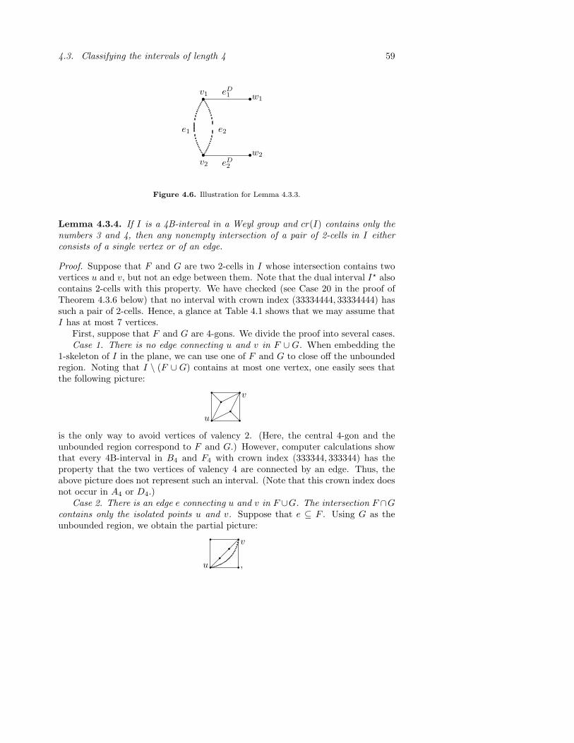
4.3. Classifying the intervals of length 4 59
r
r
r
r
v1
v2
e1 e2
eD1
eD2
w1
w2
Figure 4.6. Illustration for Lemma 4.3.3.
Lemma 4.3.4. If I is a 4B-interval in a Weyl group and cr(I) contains only thenumbers 3 and 4, then any nonempty intersection of a pair of 2-cells in I eitherconsists of a single vertex or of an edge.
Proof. Suppose that F and G are two 2-cells in I whose intersection contains twovertices u and v, but not an edge between them. Note that the dual interval I? alsocontains 2-cells with this property. We have checked (see Case 20 in the proof ofTheorem 4.3.6 below) that no interval with crown index (33334444, 33334444) hassuch a pair of 2-cells. Hence, a glance at Table 4.1 shows that we may assume thatI has at most 7 vertices.
First, suppose that F and G are 4-gons. We divide the proof into several cases.Case 1. There is no edge connecting u and v in F ∪ G. When embedding the
1-skeleton of I in the plane, we can use one of F and G to close off the unboundedregion. Noting that I \ (F ∪ G) contains at most one vertex, one easily sees thatthe following picture:
u
v
q q
q qq
q@
@
¢¢
©©
¢¢
©©
is the only way to avoid vertices of valency 2. (Here, the central 4-gon and theunbounded region correspond to F and G.) However, computer calculations showthat every 4B-interval in B4 and F4 with crown index (333344, 333344) has theproperty that the two vertices of valency 4 are connected by an edge. Thus, theabove picture does not represent such an interval. (Note that this crown index doesnot occur in A4 or D4.)
Case 2. There is an edge e connecting u and v in F ∪G. The intersection F ∩Gcontains only the isolated points u and v. Suppose that e ⊆ F . Using G as theunbounded region, we obtain the partial picture:
u
v
q q
q qq
q¡
¡¡
,
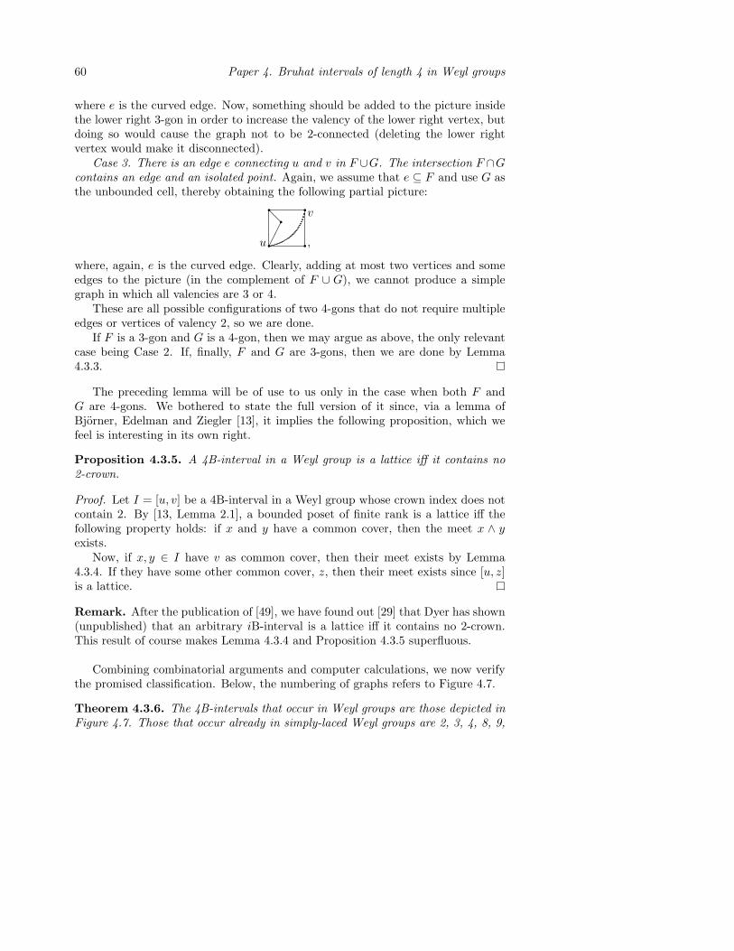
60 Paper 4. Bruhat intervals of length 4 in Weyl groups
where e is the curved edge. Now, something should be added to the picture insidethe lower right 3-gon in order to increase the valency of the lower right vertex, butdoing so would cause the graph not to be 2-connected (deleting the lower rightvertex would make it disconnected).
Case 3. There is an edge e connecting u and v in F ∪G. The intersection F ∩Gcontains an edge and an isolated point. Again, we assume that e ⊆ F and use G asthe unbounded cell, thereby obtaining the following partial picture:
u
v
q q
q qq
¢¢
@
,
where, again, e is the curved edge. Clearly, adding at most two vertices and someedges to the picture (in the complement of F ∪ G), we cannot produce a simplegraph in which all valencies are 3 or 4.
These are all possible configurations of two 4-gons that do not require multipleedges or vertices of valency 2, so we are done.
If F is a 3-gon and G is a 4-gon, then we may argue as above, the only relevantcase being Case 2. If, finally, F and G are 3-gons, then we are done by Lemma4.3.3.
The preceding lemma will be of use to us only in the case when both F andG are 4-gons. We bothered to state the full version of it since, via a lemma ofBjorner, Edelman and Ziegler [13], it implies the following proposition, which wefeel is interesting in its own right.
Proposition 4.3.5. A 4B-interval in a Weyl group is a lattice iff it contains no2-crown.
Proof. Let I = [u, v] be a 4B-interval in a Weyl group whose crown index does notcontain 2. By [13, Lemma 2.1], a bounded poset of finite rank is a lattice iff thefollowing property holds: if x and y have a common cover, then the meet x ∧ yexists.
Now, if x, y ∈ I have v as common cover, then their meet exists by Lemma4.3.4. If they have some other common cover, z, then their meet exists since [u, z]is a lattice.
Remark. After the publication of [49], we have found out [29] that Dyer has shown(unpublished) that an arbitrary iB-interval is a lattice iff it contains no 2-crown.This result of course makes Lemma 4.3.4 and Proposition 4.3.5 superfluous.
Combining combinatorial arguments and computer calculations, we now verifythe promised classification. Below, the numbering of graphs refers to Figure 4.7.
Theorem 4.3.6. The 4B-intervals that occur in Weyl groups are those depicted inFigure 4.7. Those that occur already in simply-laced Weyl groups are 2, 3, 4, 8, 9,
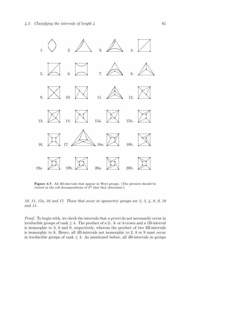
4.3. Classifying the intervals of length 4 61
1.
q
q 2. q
q
q
JJ
JJ 3. q
q
q
JJ
JJ 4. q q
q q
¡¡
¡
5. q q
q q
¡¡
¡
6. q q
q q
7. q
q
JJ
JJ©© HH 8. q
q
JJ
JJ½½
ZZ
9. q q
q qq
¡¡ @@
@@ ¡¡
10. q q
q qq
q@
@
@
¢¢
¢¢
11. q
q
qqq
JJ
JJ©©¡¡
HH@@
12. q q
q qq
q@
@
@
¢¢
¢¢
©©
13. q q
q qq
q@
@
@
¢¢
©©
¢¢
©©
14. q q
q qq
q q@
@
@ ¡
¢¢
15a. q q
q qq
¡
@ ¢¢
©©
@@
15b. q q
q qq
q q©©@
@ ©©
¢¢
¡
16. q q
q qq qq q
¡ @
¡@
17. q
q
qqq q
¶¶
¶¶S
SS
S½½
³³³Z
ZPPP
LLL
¯¯H©
18a. q q
q qq
q q¢¢
©©
@HH¡¢¢@ 18b. q q
q qq
q q©©
@ ¡©©
@AA@
19a. q q
q qq qq q
¡©©
@ ©©
AA
19b. q q
q qq qq q
¡©©
AA
©©
AA
20a. q q
q qq qq q
¡
@
©©
AA
©©
AA
20b. q q
q qq qq q
¡ @
¡@
©©
HH
Figure 4.7. All 4B-intervals that appear in Weyl groups. (The pictures should beviewed as the cell decompositions of S2 that they determine.)
10, 11, 15a, 16 and 17. Those that occur in symmetric groups are 2, 3, 4, 8, 9, 10and 11.
Proof. To begin with, we check the intervals that a priori do not necessarily occur inirreducible groups of rank ≤ 4. The product of a 2-, 3- or 4-crown and a 1B-intervalis isomorphic to 2, 8 and 9, respectively, whereas the product of two 2B-intervalsis isomorphic to 8. Hence, all 4B-intervals not isomorphic to 2, 8 or 9 must occurin irreducible groups of rank ≤ 4. As mentioned before, all 4B-intervals in groups

62 Paper 4. Bruhat intervals of length 4 in Weyl groups
of rank < 4 also appear in groups of rank 4. It remains to check the 4B-intervalsin A4, B4, D4 and F4.
For each crown index in Table 4.1, we classify the 4B-intervals that give rise toit. We omit the cases 4, 7, 11, 14, 17 and 19, since they are obtained by dualityfrom 3, 6, 10, 13, 16 and 18, respectively.
1. cr(I) = (22, 22):Clearly, 1 is the only decomposition of S2 into two 2-gons.
2. cr(I) = (233, 233):Choosing a 3-cycle to close off the unbounded region, 2 is the only possible way toembed in the plane a graph with the prescribed valencies.
3. cr(I) = (334, 2233):Again, choosing a 3-cycle to close off the unbounded region, the only possible loop-free graph is 3.
5. cr(I) = (2334, 2334):Pick a 4-cycle v1, v2, v3, v4, v1 to close off the unbounded region. There is one ver-tex, say v1, with valency 4. The two remaining edges emanating from it end atdifferent vertices (otherwise we would have another valency 4 vertex). If these werev2 and v4, the crown index would be (2334, 2244). Hence, v3 has valency 3, making5 the only possible picture.
6. cr(I) = (3333, 2244):Let a 4-cycle close off the unbounded region. Each vertex is contained in one moreedge. No diagonal edges can occur; this would force edges to cross. Hence, 6 is theremaining possibility.
In the remaining cases, we will implicitly use that there can be no multiple edgesas ensured by Lemma 4.3.3.
8. cr(I) = (3333, 3333):The underlying graph must be the complete graph K4. The only way to embed itin the plane is 8.
9. cr(I) = (33334, 33334):Choose a 4-cycle to close off the unbounded region. No diagonal edges in the 4-cycleare possible since they would force the “isolated” vertex to have valency 2. Hencethe remaining four edges must all have one endpoint in the middle vertex. Theresult is 9.
10. cr(I) = (333333, 33444):

4.3. Classifying the intervals of length 4 63
Close off the unbounded region with a 4-cycle. Since all vertices have valency 3and there are 5 remaining edges, the middle vertices must be connected by an edge.The remaining two edges from each middle vertex must end in adjacent edges onthe outer 4-cycle; otherwise a vertex in the outer 4-cycle would be forced to havevalency 2. The only possibility left is 10.
12. cr(I) = (333344, 333344):Pick a 4-cycle to close off the unbounded region. There is one other 4-gon andtwo more vertices. Hence, the intersection of the two 4-gons must be an edge, byLemma 4.3.4. Now, 12 is the only possibility.
13. cr(I) = (334444, 3333334):As usual, let the unbounded region be a 4-gon. Vertices of valency 4 on the outer4-cycle necessarily have edges to both inner vertices. Therefore, two vertices thatare adjacent on the outer 4-cycle cannot both have valency 4; this would mean thatone of the inner vertices must have valency 2 or (if the inner vertices are connectedby an edge) that one of the remaining vertices on the outer 4-cycle must have va-lency 2. Hence, the four vertices of valency 4 are two diagonal vertices on the outer4-cycle and both inner vertices, forcing the situation to be as in 13.
15. cr(I) = (3333444, 3333444):There are seven vertices, so each pair of 4-gons has nonempty intersection. ByLemma 4.3.4, either each such pair intersects in an edge, or there is a pair of 4-gonsthat intersect in a single vertex.
First suppose that every 4-gon pair intersects in an edge. Let the unboundedregion be a 4-gon. Then the two edges that intersect the other 4-gons are are eitherdisjoint or not. The former case implies this appearance:
q q
q qqq
q¡
¡¢¢
@HH ¢¢@ .
In the latter case, we have the following partial picture:
q q
q qq qq
¡ @
@
.
The only way to fill in three more edges without destroying one of the 4-gons orgetting forbidden valencies is 15a.
Now suppose that there is a pair of 4-gons intersecting in a single vertex. Usingone of them as the unbounded region, we get the partial picture:
q q
q qq
q q¢¢
©© .
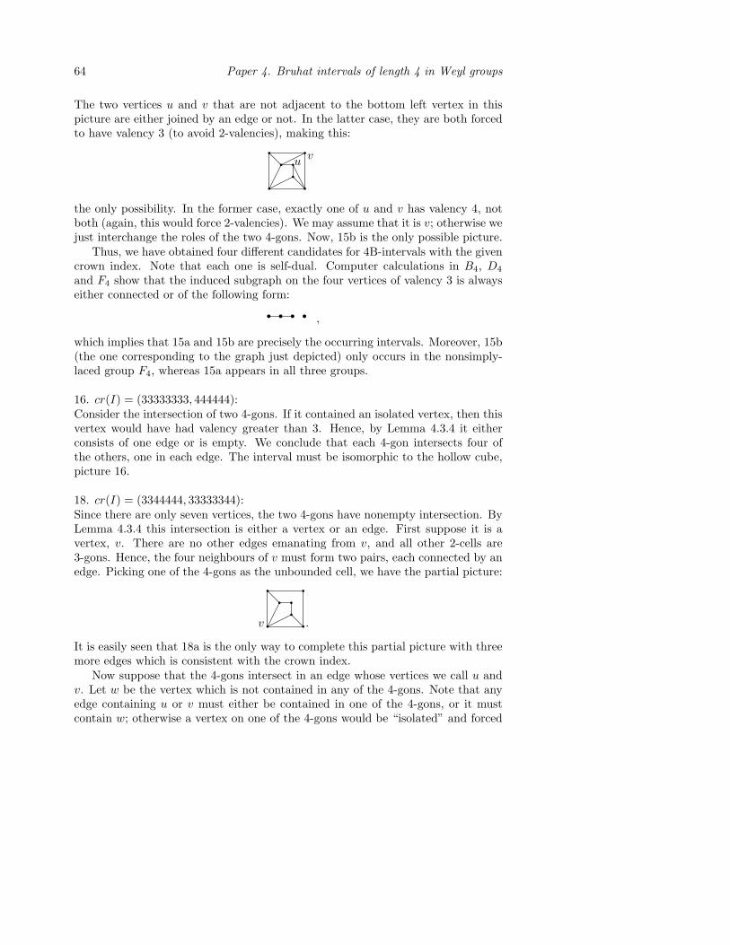
64 Paper 4. Bruhat intervals of length 4 in Weyl groups
The two vertices u and v that are not adjacent to the bottom left vertex in thispicture are either joined by an edge or not. In the latter case, they are both forcedto have valency 3 (to avoid 2-valencies), making this:
vu
q q
q qq
q q¢¢
©©
@ ©©
@AA
the only possibility. In the former case, exactly one of u and v has valency 4, notboth (again, this would force 2-valencies). We may assume that it is v; otherwise wejust interchange the roles of the two 4-gons. Now, 15b is the only possible picture.
Thus, we have obtained four different candidates for 4B-intervals with the givencrown index. Note that each one is self-dual. Computer calculations in B4, D4
and F4 show that the induced subgraph on the four vertices of valency 3 is alwayseither connected or of the following form:
r r r r ,
which implies that 15a and 15b are precisely the occurring intervals. Moreover, 15b(the one corresponding to the graph just depicted) only occurs in the nonsimply-laced group F4, whereas 15a appears in all three groups.
16. cr(I) = (33333333, 444444):Consider the intersection of two 4-gons. If it contained an isolated vertex, then thisvertex would have had valency greater than 3. Hence, by Lemma 4.3.4 it eitherconsists of one edge or is empty. We conclude that each 4-gon intersects four ofthe others, one in each edge. The interval must be isomorphic to the hollow cube,picture 16.
18. cr(I) = (3344444, 33333344):Since there are only seven vertices, the two 4-gons have nonempty intersection. ByLemma 4.3.4 this intersection is either a vertex or an edge. First suppose it is avertex, v. There are no other edges emanating from v, and all other 2-cells are3-gons. Hence, the four neighbours of v must form two pairs, each connected by anedge. Picking one of the 4-gons as the unbounded cell, we have the partial picture:
v q q
q qq
q q¢¢
©©
@
@ .
It is easily seen that 18a is the only way to complete this partial picture with threemore edges which is consistent with the crown index.
Now suppose that the 4-gons intersect in an edge whose vertices we call u andv. Let w be the vertex which is not contained in any of the 4-gons. Note that anyedge containing u or v must either be contained in one of the 4-gons, or it mustcontain w; otherwise a vertex on one of the 4-gons would be “isolated” and forced
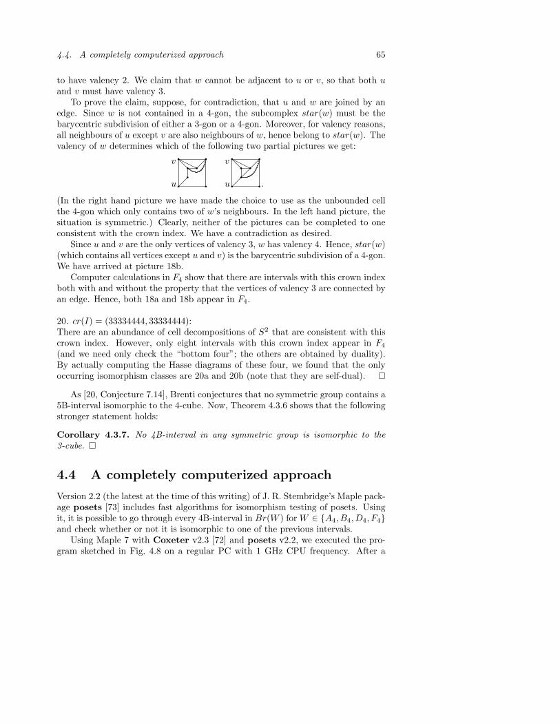
4.4. A completely computerized approach 65
to have valency 2. We claim that w cannot be adjacent to u or v, so that both uand v must have valency 3.
To prove the claim, suppose, for contradiction, that u and w are joined by anedge. Since w is not contained in a 4-gon, the subcomplex star(w) must be thebarycentric subdivision of either a 3-gon or a 4-gon. Moreover, for valency reasons,all neighbours of u except v are also neighbours of w, hence belong to star(w). Thevalency of w determines which of the following two partial pictures we get:
v
u q q
q qqq q
¡
@HH¡ v
u q q
q qqq q
¡
@HH¡¡
.
(In the right hand picture we have made the choice to use as the unbounded cellthe 4-gon which only contains two of w’s neighbours. In the left hand picture, thesituation is symmetric.) Clearly, neither of the pictures can be completed to oneconsistent with the crown index. We have a contradiction as desired.
Since u and v are the only vertices of valency 3, w has valency 4. Hence, star(w)(which contains all vertices except u and v) is the barycentric subdivision of a 4-gon.We have arrived at picture 18b.
Computer calculations in F4 show that there are intervals with this crown indexboth with and without the property that the vertices of valency 3 are connected byan edge. Hence, both 18a and 18b appear in F4.
20. cr(I) = (33334444, 33334444):There are an abundance of cell decompositions of S2 that are consistent with thiscrown index. However, only eight intervals with this crown index appear in F4
(and we need only check the “bottom four”; the others are obtained by duality).By actually computing the Hasse diagrams of these four, we found that the onlyoccurring isomorphism classes are 20a and 20b (note that they are self-dual).
As [20, Conjecture 7.14], Brenti conjectures that no symmetric group contains a5B-interval isomorphic to the 4-cube. Now, Theorem 4.3.6 shows that the followingstronger statement holds:
Corollary 4.3.7. No 4B-interval in any symmetric group is isomorphic to the3-cube. ¤
4.4 A completely computerized approach
Version 2.2 (the latest at the time of this writing) of J. R. Stembridge’s Maple pack-age posets [73] includes fast algorithms for isomorphism testing of posets. Usingit, it is possible to go through every 4B-interval in Br(W ) for W ∈ A4, B4, D4, F4and check whether or not it is isomorphic to one of the previous intervals.
Using Maple 7 with Coxeter v2.3 [72] and posets v2.2, we executed the pro-gram sketched in Fig. 4.8 on a regular PC with 1 GHz CPU frequency. After a

66 Paper 4. Bruhat intervals of length 4 in Weyl groups
for each W in A4, D4, B4, F4 do
S ← ∅
for each [u, v] ⊆ Br(W ) with`(v)− `(u) = 4 and `(u) ≤ `(Br(W ))/2− 2 do
if [u, v] is not isomorphic to any I in S then
S ← S ∪ [u, v],dual([u, v])
remove isomorphic copies from S
output S
Figure 4.8. Sketch of the program used to compute all 4B-intervals in A4, B4, D4
and F4. As usual, we only go through the lower half of each Bruhat order, obtainingthe upper by duality.
few days of running time, we obtained the following output. The program found7, 10, 17 and 24 different intervals in A4, D4, B4 and F4, respectively, in completeagreement with Theorem 4.3.6.
Although beyond the scope of this article, we note that it could well be possibleto perform an exhaustive search along the lines just described also for 5B-intervals.In this case, the relevant groups of rank 5 are A5, B5 and D5. One would also haveto check F4, since it is not contained in the others as a parabolic subgroup.
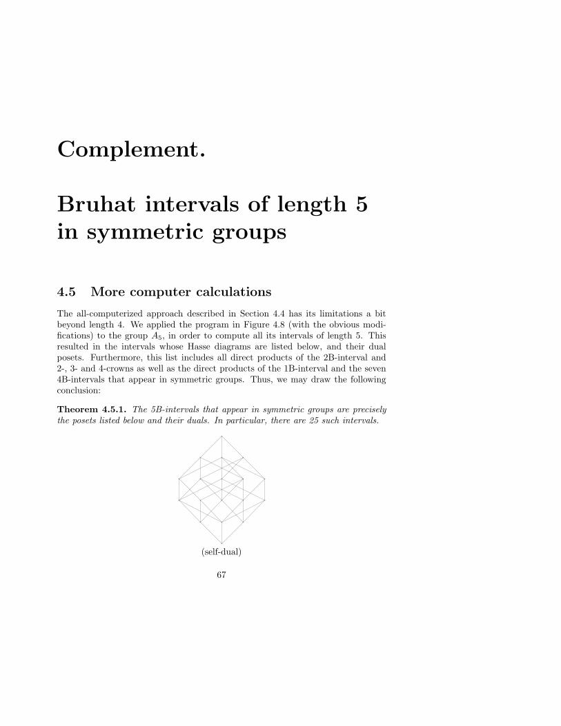
Complement.
Bruhat intervals of length 5in symmetric groups
4.5 More computer calculations
The all-computerized approach described in Section 4.4 has its limitations a bitbeyond length 4. We applied the program in Figure 4.8 (with the obvious modi-fications) to the group A5, in order to compute all its intervals of length 5. Thisresulted in the intervals whose Hasse diagrams are listed below, and their dualposets. Furthermore, this list includes all direct products of the 2B-interval and2-, 3- and 4-crowns as well as the direct products of the 1B-interval and the seven4B-intervals that appear in symmetric groups. Thus, we may draw the followingconclusion:
Theorem 4.5.1. The 5B-intervals that appear in symmetric groups are preciselythe posets listed below and their duals. In particular, there are 25 such intervals.
(self-dual)
67
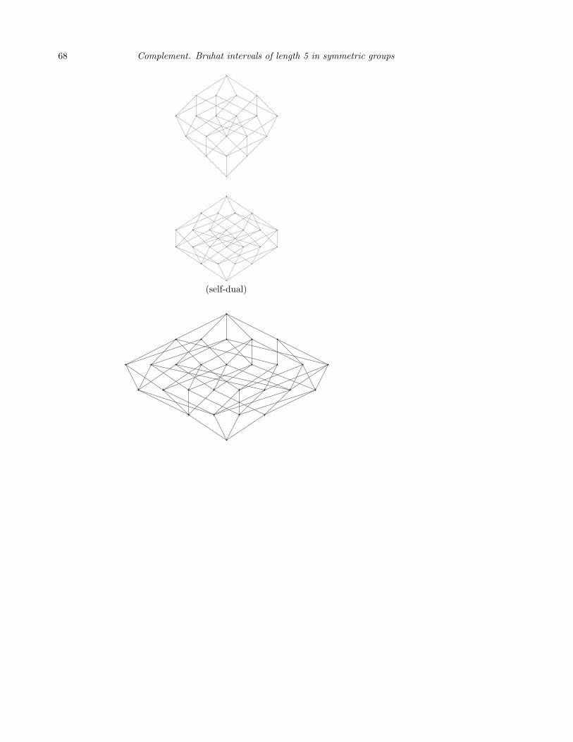
68 Complement. Bruhat intervals of length 5 in symmetric groups
(self-dual)
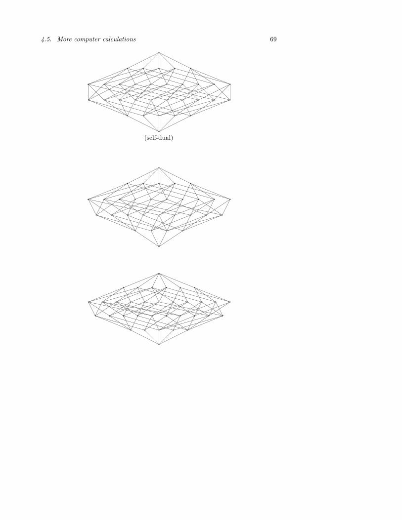
4.5. More computer calculations 69
(self-dual)
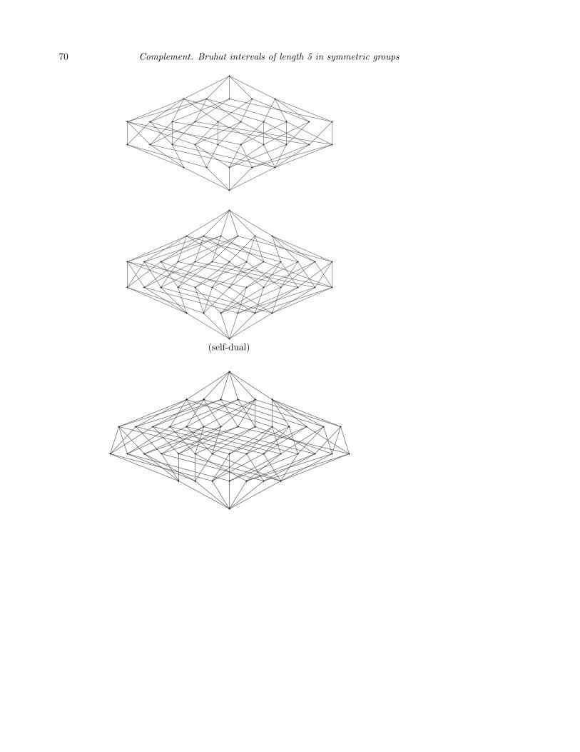
70 Complement. Bruhat intervals of length 5 in symmetric groups
(self-dual)
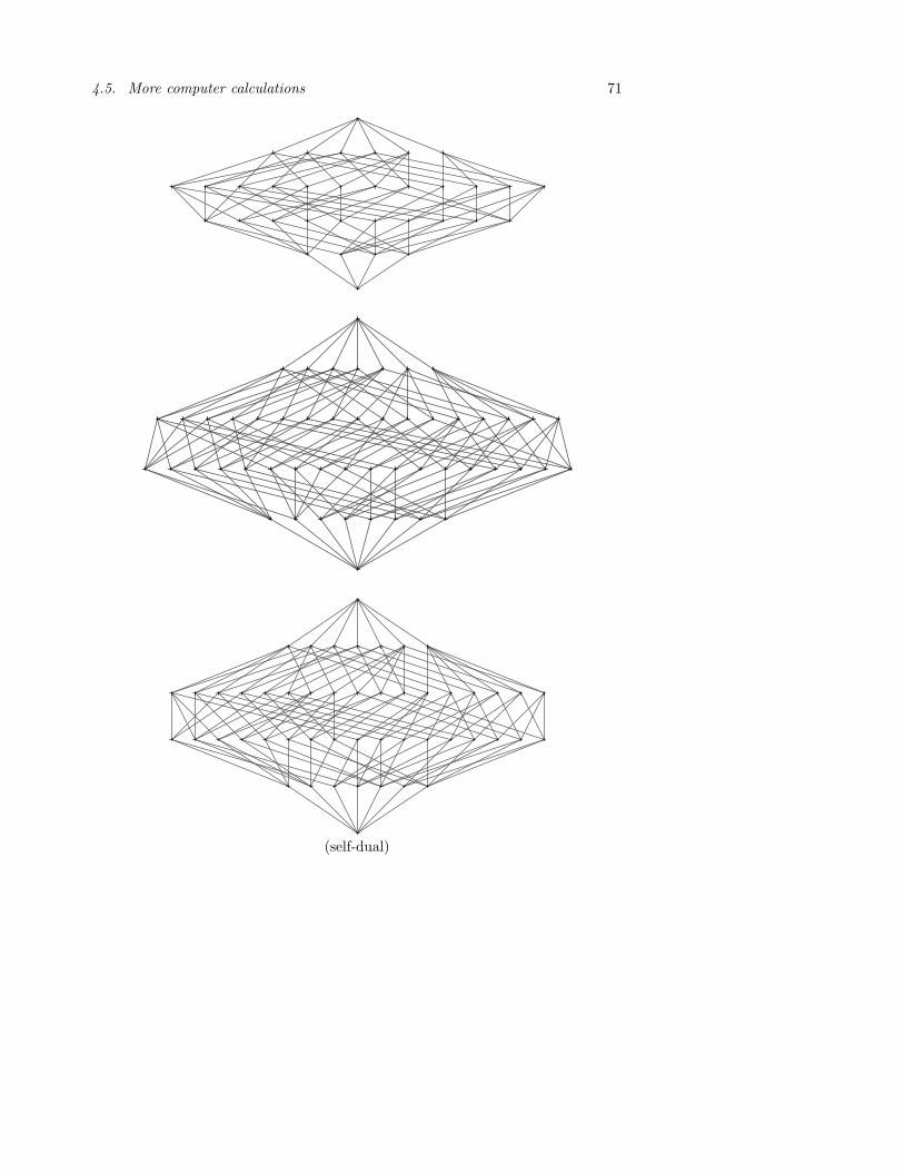
4.5. More computer calculations 71
(self-dual)
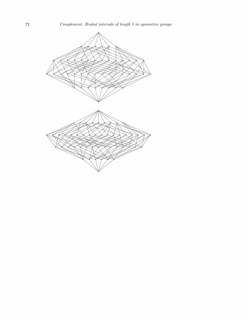
72 Complement. Bruhat intervals of length 5 in symmetric groups
Part III
Expected reflection distances
73

74
Paper 5.
Estimating the expectedreversal distance after trandom reversals
5.1 Introduction
Over the last decade, the computational biology community has been looking at theproblem of estimating evolutionary distances between taxa from their gene order.The probably most common, and by far most studied, evolutionary operation inthis context is the reversal: a segment (that is a sequence of consecutive genes)of the genome is taken out and inserted at the same place, but in reversed order.In 1995, Hannenhalli and Pevzner [44] presented a formula for the minimal num-ber of reversals needed to transform one sequence of distinct genes into a givenpermutation of them.
For distant genomes, the true evolutionary distance is in general much longerthan the shortest distance. In order to find a better estimate of the true distance,we may instead look at the expected distance. Such attempts have been made byWang [76] and Eriksen [30], providing bounds for, and an approximation of, theexpected reversal distance given the number of breakpoints between two genomes πand τ . (There is a breakpoint between two genes in π if they are adjacent in π butnot in τ .)
The reversal distance “contains more information” than the breakpoint distance,so if we could find the expected reversal distance, we would probably obtain abiologically more relevant formula. For the same reasons, we would also expectthis problem to be harder. The inverse problem seems to be of more reasonabledifficulty:
75
76 Paper 5. Estimating the expected reversal distance after t random reversals
Problem 5.1.1. Compute the expected reversal distance after t random reversals,taken independently from a uniform distribution.
In this paper (Section 5.3), we find an analogy between certain cycles used byHannenhalli and Pevzner, and the ordinary cycles in the symmetric group. Wereach the conclusion that one can obtain a good estimate to the expected reversaldistance by solving the following analogous problem:
Problem 5.1.2. Compute the expected transposition distance in the symmetricgroup after t random transpositions.
In Sections 5.4 and 5.5 we find the solution to Problem 5.1.2 to be the followingformula:
Etrp(n, t) = n−n∑
k=1
1k
+n−1∑p=1
min(p,n−p)∑q=1
apq
((p2
)+
(q−12
)− (n−p−q+2
2
)(n2
))t
, (5.1)
where
apq = (−1)n−p−q+1 (p− q + 1)2
(n− q + 1)2(n− p)
(n− p− 1
q − 1
)(n
p
).
Finally, in Section 5.6 we show how the inverse of (5.1) can be used as an estimatefor the expected evolutionary reversal distance and investigate numerically how wellthis formula behaves compared to previous methods when it comes to predictingthe true evolutionary distance.
It should be noted that “expected reversal distances” have been studied as earlyas in 1996 [4]. That paper, however, dealt with the expected reversal distance of alinear, unsigned genome taken from the uniform distribution.
Remark. In [32], we use analogous, but somewhat more involved, methods to solveProblem 5.1.2 for the complex reflection groups G(r, 1, n). The symmetric groupis then the special case r = 1. For r > 1, there are no immediate applications tocomputational biology.
Acknowledgement. The authors are most grateful to Richard Stanley for point-ing out a way to prove Theorem 5.5.1. We also thank Kimmo Eriksson for hiscareful reading of this article.
5.2 Preliminaries
Let Sn be the symmetric group on n elements and let dtrp(π) be the minimaltransposition distance from a permutation π to the identity permutation, i.e. theminimal i such that π is a product of i transpositions. It is well-known since Cayleythat dtrp(π) = n− ctrp(π), where ctrp(π) is the number of cycles in π.
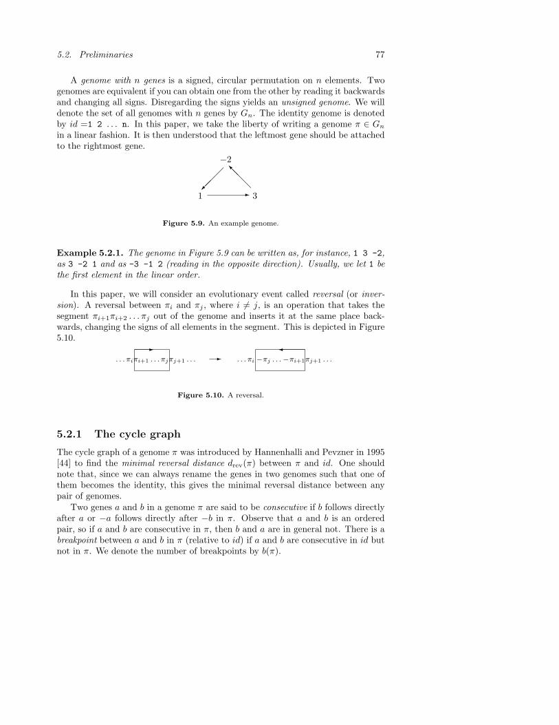
5.2. Preliminaries 77
A genome with n genes is a signed, circular permutation on n elements. Twogenomes are equivalent if you can obtain one from the other by reading it backwardsand changing all signs. Disregarding the signs yields an unsigned genome. We willdenote the set of all genomes with n genes by Gn. The identity genome is denotedby id =1 2 . . . n. In this paper, we take the liberty of writing a genome π ∈ Gn
in a linear fashion. It is then understood that the leftmost gene should be attachedto the rightmost gene.
1 3
−2
-
¡¡¡ª @
@@I
Figure 5.9. An example genome.
Example 5.2.1. The genome in Figure 5.9 can be written as, for instance, 1 3 -2,as 3 -2 1 and as -3 -1 2 (reading in the opposite direction). Usually, we let 1 bethe first element in the linear order.
In this paper, we will consider an evolutionary event called reversal (or inver-sion). A reversal between πi and πj , where i 6= j, is an operation that takes thesegment πi+1πi+2 . . . πj out of the genome and inserts it at the same place back-wards, changing the signs of all elements in the segment. This is depicted in Figure5.10.
. . . πiπi+1 . . . πjπj+1 . . . - . . . πi −πj . . .−πi+1πj+1 . . .
- ¾
Figure 5.10. A reversal.
5.2.1 The cycle graph
The cycle graph of a genome π was introduced by Hannenhalli and Pevzner in 1995[44] to find the minimal reversal distance drev(π) between π and id. One shouldnote that, since we can always rename the genes in two genomes such that one ofthem becomes the identity, this gives the minimal reversal distance between anypair of genomes.
Two genes a and b in a genome π are said to be consecutive if b follows directlyafter a or −a follows directly after −b in π. Observe that a and b is an orderedpair, so if a and b are consecutive in π, then b and a are in general not. There is abreakpoint between a and b in π (relative to id) if a and b are consecutive in id butnot in π. We denote the number of breakpoints by b(π).
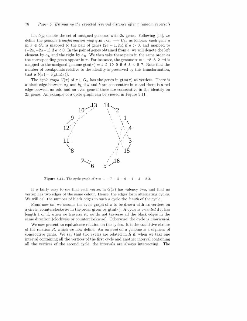
78 Paper 5. Estimating the expected reversal distance after t random reversals
Let U2n denote the set of unsigned genomes with 2n genes. Following [44], wedefine the genome transformation map gtm : Gn −→ U2n as follows: each gene ain π ∈ Gn is mapped to the pair of genes (2a − 1, 2a) if a > 0, and mapped to(−2a,−2a−1) if a < 0. In the pair of genes obtained from a, we will denote the leftelement by aL and the right by aR. We then take these pairs in the same order asthe corresponding genes appear in π. For instance, the genome π = 1 -5 3 2 -4 ismapped to the unsigned genome gtm(π) = 1 2 10 9 5 6 3 4 8 7. Note that thenumber of breakpoints relative to the identity is preserved by this transformation,that is b(π) = b(gtm(π)).
The cycle graph G(π) of π ∈ Gn has the genes in gtm(π) as vertices. There isa black edge between aR and bL if a and b are consecutive in π and there is a rededge between an odd and an even gene if these are consecutive in the identity on2n genes. An example of a cycle graph can be viewed in Figure 5.11.
142
1
4
109
12
15
567
8
11
16
3
13
Figure 5.11. The cycle graph of π = 1 − 7 − 5 − 6 − 4 − 3 − 8 2.
It is fairly easy to see that each vertex in G(π) has valency two, and that novertex has two edges of the same colour. Hence, the edges form alternating cycles.We will call the number of black edges in such a cycle the length of the cycle.
From now on, we assume the cycle graph of π to be drawn with its vertices ona circle, counterclockwise in the order given by gtm(π). A cycle is oriented if it haslength 1 or if, when we traverse it, we do not traverse all the black edges in thesame direction (clockwise or counterclockwise). Otherwise, the cycle is unoriented.
We now present an equivalence relation on the cycles. It is the transitive closureof the relation R, which we now define. An interval on a genome is a segment ofconsecutive genes. We say that two cycles are related in R if, when we take oneinterval containing all the vertices of the first cycle and another interval containingall the vertices of the second cycle, the intervals are always intersecting. The

5.3. The analogy 79
equivalence classes are called components. A component is oriented if it containsat least one oriented cycle and unoriented otherwise.
If there is an interval that contains (the vertices of) an unoriented componentτ , but no other unoriented components, then τ is known as a hurdle. If there isan interval which contains exactly two unoriented components and possibly someoriented ones, and exactly one of these unoriented components is a hurdle, thenthis hurdle is a super hurdle. Finally, if a cycle graph contains an odd number ofhurdles, all of which are super hurdles, then this graph is known as a fortress.
For π ∈ Gn, we define crev(π) to be the number of cycles in G(π). Similarly, h(π)is its number of hurdles. Finally, f(π) is one if G(π) is a fortress, zero otherwise.Using these functions, we can formulate the theorem of Hannenhalli and Pevzner.
Theorem 5.2.2 ([44]). The minimal reversal distance is given by
drev(π) = n− crev(π) + h(π) + f(π).
It follows from Caprara [21] that genomes containing hurdles are very rare. Forinstance, for genomes of length 8, less than one percent of these contain hurdles,and for genomes of length 100, only one in 105 contains a hurdle. Thus, there islittle harm in using the approximation drev(π) ≈ n − crev(π), observing that thisformula is very similar to the one governing transposition distance in Sn.
5.3 The analogy
We shall now explore the analogy between unsigned transpositions and signed re-versals. If we apply a transposition τ = (a b) to a permutation π ∈ Sn, one of thefollowing things will happen.
• If a and b belong to different cycles in π, the number of cycles will decreaseby one.
• If a and b belong the same cycle in π, the number of cycles will increase byone.
Thus, applying a transposition to π will change the transposition distance by one.On the other hand, if we apply the reversal a . . . b to π ∈ Gn, one of the following
things will happen.
• If aL and bR belong to different cycles in gtm(π), the number of cycles willdecrease by one.
• If aL and bR belong to the same cycle and the black edges connected to aL
and bR are traversed in different directions when we traverse this cycle, thenumber of cycles will increase by one.
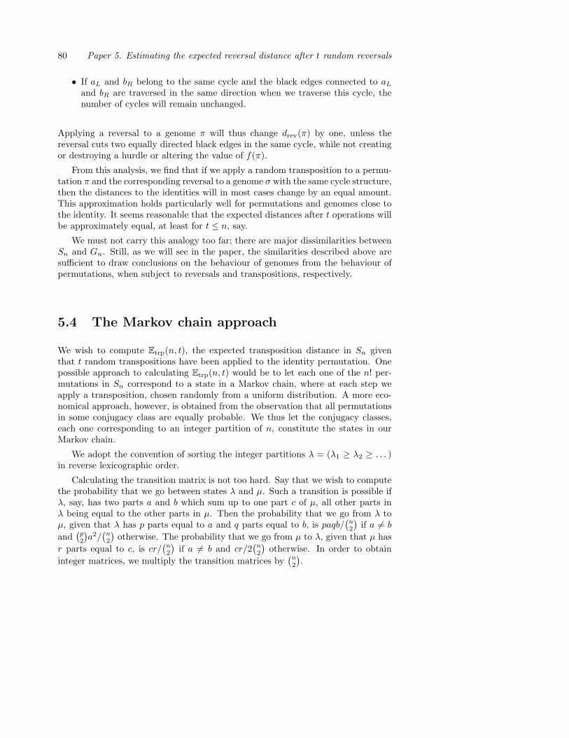
80 Paper 5. Estimating the expected reversal distance after t random reversals
• If aL and bR belong to the same cycle and the black edges connected to aL
and bR are traversed in the same direction when we traverse this cycle, thenumber of cycles will remain unchanged.
Applying a reversal to a genome π will thus change drev(π) by one, unless thereversal cuts two equally directed black edges in the same cycle, while not creatingor destroying a hurdle or altering the value of f(π).
From this analysis, we find that if we apply a random transposition to a permu-tation π and the corresponding reversal to a genome σ with the same cycle structure,then the distances to the identities will in most cases change by an equal amount.This approximation holds particularly well for permutations and genomes close tothe identity. It seems reasonable that the expected distances after t operations willbe approximately equal, at least for t ≤ n, say.
We must not carry this analogy too far; there are major dissimilarities betweenSn and Gn. Still, as we will see in the paper, the similarities described above aresufficient to draw conclusions on the behaviour of genomes from the behaviour ofpermutations, when subject to reversals and transpositions, respectively.
5.4 The Markov chain approach
We wish to compute Etrp(n, t), the expected transposition distance in Sn giventhat t random transpositions have been applied to the identity permutation. Onepossible approach to calculating Etrp(n, t) would be to let each one of the n! per-mutations in Sn correspond to a state in a Markov chain, where at each step weapply a transposition, chosen randomly from a uniform distribution. A more eco-nomical approach, however, is obtained from the observation that all permutationsin some conjugacy class are equally probable. We thus let the conjugacy classes,each one corresponding to an integer partition of n, constitute the states in ourMarkov chain.
We adopt the convention of sorting the integer partitions λ = (λ1 ≥ λ2 ≥ . . . )in reverse lexicographic order.
Calculating the transition matrix is not too hard. Say that we wish to computethe probability that we go between states λ and µ. Such a transition is possible ifλ, say, has two parts a and b which sum up to one part c of µ, all other parts inλ being equal to the other parts in µ. Then the probability that we go from λ toµ, given that λ has p parts equal to a and q parts equal to b, is paqb/
(n2
)if a 6= b
and(p2
)a2/
(n2
)otherwise. The probability that we go from µ to λ, given that µ has
r parts equal to c, is cr/(n2
)if a 6= b and cr/2
(n2
)otherwise. In order to obtain
integer matrices, we multiply the transition matrices by(n2
).
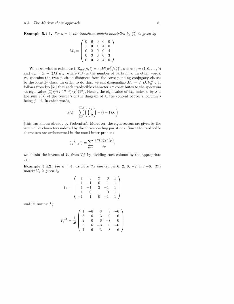
5.4. The Markov chain approach 81
Example 5.4.1. For n = 4, the transition matrix multiplied by(n2
)is given by
M4 =
0 6 0 0 01 0 1 4 00 2 0 0 40 3 0 0 30 0 2 4 0
What we wish to calculate is Etrp(n, t) = e1MtnwT
n /(n2
)t, where e1 = (1, 0, . . . , 0)and wn = (n − `(λ))λ`n, where `(λ) is the number of parts in λ. In other words,wn contains the transposition distances from the corresponding conjugacy classesto the identity class. In order to do this, we can diagonalize Mn = VnDnV −1
n . Itfollows from Ito [51] that each irreducible character χλ contributes to the spectruman eigenvalue
(n2
)χλ(2, 1n−2)/χλ(1n), Hence, the eigenvalue of Mn indexed by λ is
the sum c(λ) of the contents of the diagram of λ, the content of row i, column jbeing j − i. In other words,
c(λ) =`(λ)∑
i=1
((λi
2
)− (i− 1)λi
)
(this was known already by Frobenius). Moreover, the eigenvectors are given by theirreducible characters indexed by the corresponding partitions. Since the irreduciblecharacters are orthonormal in the usual inner product
〈χλ, χν〉 =∑
µ`n
χλ(µ)χν(µ)zµ
,
we obtain the inverse of Vn from V Tn by dividing each column by the appropriate
zλ.
Example 5.4.2. For n = 4, we have the eigenvalues 6, 2, 0, −2 and −6. Thematrix V4 is given by
V4 =
1 3 2 3 1−1 −1 0 1 1
1 −1 2 −1 11 0 −1 0 1
−1 1 0 −1 1
and its inverse by
V −14 =
14!
1 −6 3 8 −63 −6 −3 0 62 0 6 −8 03 6 −3 0 −61 6 3 8 6

82 Paper 5. Estimating the expected reversal distance after t random reversals
With this information, we find that
e1MtnwT
n =∑
λ`n
χλ(1n)
(c(λ)(
n2
))t ∑
µ`n
χλ(µ)wµ
zµ
Theorem 5.4.3. If λ3 ≥ 2, then∑
µ`n
χλ(µ)wµ
zµ= 0.
Otherwise, let λ = (p, q, 1n−p−q). Then, for p, q ≥ 1,∑
µ`n
χλ(µ)wµ
zµ= (−1)n−p−q+1 p− q + 1
(n− q + 1)(n− p),
and, for p = n, q = 0,∑
µ`n
χ(n)(µ)wµ
zµ= n−
n∑
k=1
1k
.
We postpone the proof of this theorem to Subsection 5.5.1. Using it, we cangive a closed formula for the expected transposition distance after t random trans-positions in Sn.
Corollary 5.4.4. The expected transposition distance after t random transpositionsin Sn is given by
n−n∑
k=1
1k
+n−1∑p=1
min(p,n−p)∑q=1
apq
((p2
)+
(q−12
)− (n−p−q+2
2
)(n2
))t
,
where
apq = (−1)n−p−q+1 (p− q + 1)2
(n− q + 1)2(n− p)
(n− p− 1
q − 1
)(n
p
).
Proof. The character χλ(1n) is given (see [60] or [70]) by the hook-length formula
χλ(1n) =n!∏
c∈λ hc
For λ = (p, q, 1n−p−q), this yields
χλ(1n) =n!(p− q + 1)
(q − 1)!(n− p− q)!(n− p)(n− q + 1)p!
=(p− q + 1)(n− q + 1)
(n− p− 1
q − 1
)(n
p
).
Since the sum of the contents of such a partition is(
p
2
)+
(q − 1
2
)−
(n− p− q + 2
2
),
the corollary follows.
5.5. Decomposing the length function 83
Of interest is the behaviour of the expected distance as t grows (keeping n fixed).Depending on the parity of t, one of two limits is approached. It is not surprisingthat what we obtain for even (odd) t is exactly the expected distance of a randomlychosen even (odd) permutation of [n] from a uniform distribution. We leave theverification of this statement to the reader.
Corollary 5.4.5. We have
limt→∞
Etrp(n, 2t) = n−n∑
k=1
1k
+ (−1)n−1 1n(n− 1)
and
limt→∞
Etrp(n, 2t + 1) = n−n∑
k=1
1k
+ (−1)n 1n(n− 1)
.
Proof. As t grows, all terms but one in the double sum of Corollary 5.4.4 tendto zero, the exception being given by p = q = 1. This term is (−1)t+n−1 1
n(n−1) .Substituting 2t and 2t + 1, respectively, for t yields the result.
5.5 Decomposing the length function
Recall that the length, `(λ), of a partition λ is its number of parts. In this sectionwe will use elements of symmetric functions theory in order to prove our maintechnical tool: a decomposition formula for `. To this end, we briefly review thematerial we need. For terminology not explained here, we refer the reader e.g. toMacdonald [60] or Stanley [70, Chapter 7].
Let Rn be the vector space (over Q, say) of class functions, i.e. functionsf : Pn −→ Q, where Pn is the set of integer partitions of n. The irreducibleSn-characters, χλλ`n form an orthonormal basis of Rn with respect to the innerproduct defined by 〈f, g〉 = 1
n!
∑π∈Sn
f(type(π))g(type(π)). As a vector space, Rn
is isomorphic to the space Λn of symmetric functions of degree n via the character-istic map, chn : Rn −→ Λn, defined by f 7→ ∑
λ`npλ
zλf(λ). Here, n!
zλis the number
of permutations of cycle type λ in Sn and pλλ`n is the Λn-basis of power sums.We will use one more basis of Λn. The Schur function sλ is the image of χλ underchn, hence the Schur functions form a basis.
If λ and µ are two partitions such that the Ferrers diagram of λ is contained inthat of µ, then µ/λ denotes the part of the µ-diagram not contained in λ. We callµ/λ a border strip if it is connected (meaning that we can walk from any square toany other without crossing corners) and contains no 2 × 2 subsquare. The height,ht(µ/λ), of the border strip µ/λ is one less than the number of rows in its diagram.
Richard Stanley pointed out to us the usefulness of the following two equationsto proving Theorem 5.5.1 below. Letting the first t y-variables be equal to one and
84 Paper 5. Estimating the expected reversal distance after t random reversals
the rest be zero in [70, 7.20], then differentiating with respect to t, putting t = 1and considering only terms of degree n yields
∑
λ`n
`(λ)zλ
pλ =n∑
k=1
1k
s(n−k)p(k). (5.2)
The following is a special case of [70, 7.72]. The sum is over all λ ` n such thatλ/(n− k) is a border strip.
s(n−k)p(k) =∑
λ
(−1)ht(λ/(n−k))sλ. (5.3)
We are now ready to prove the theorem.
Theorem 5.5.1. Let λ ` n. We have `(λ) =∑
µ`n cµχµ(λ), where
cµ =
∑nk=1
1k if µ = (n),
(−1)n−p−q p−q+1(n−q+1)(n−p) if µ = (p, q, 1n−p−q),
0 otherwise.
Proof. Living in Rn, ` can be written uniquely as a linear combination of theχµµ`n. Hence, ` =
∑cµχµ for some coefficients cµ. Passing to Λn yields
∑
µ`n
cµsµ =∑
µ`n
pµ
zµ`(µ).
Using (5.2), we get∑
µ`n
cµsµ =n∑
k=1
1k
s(n−k)p(k),
which, with the aid of (5.3), turns into
∑
µ`n
cµsµ =n∑
k=1
∑µ
1k
(−1)ht(µ/(n−k))sµ,
so thatcµ =
∑ 1k
(−1)ht(µ/(n−k)),
where the sum now is over all k such that µ/(n − k) is a border strip. Thisimmediately shows that cµ = 0 unless µ = (n) or µ = (p, q, 1n−p−q) for some p ≥q ≥ 1. Now, (n)/(n− k) is always a border strip of height zero, so c(n) =
∑nk=1
1k .
Finally, (p, q, 1n−p−q)/(n − k) is a border strip if and only if q = n − k + 1 orp = n− k. Thus,
c(p,q,1n−p−q) = (−1)n−p−q+1 1n− q + 1
+ (−1)n−p−q 1n− p
= (−1)n−p−q p− q + 1(n− q + 1)(n− p)
.
5.5. Decomposing the length function 85
5.5.1 Proof of Theorem 5.4.3
Now we show that Theorem 5.4.3 is a consequence of Theorem 5.5.1. Note thatµ 7→ wµ is a class function and that for fixed λ ` n we have
∑
µ`n
χλ(µ)wµ
zµ= 〈χλ, w•〉.
Hence,∑
µ`nχλ(µ)wµ
zµis the coefficient of χλ when the class function w• is written
as a linear combination of the irreducible Sn-characters. Now, wµ = n − `(µ).Hence, with cµ as in Theorem 5.5.1, the coefficient of the trivial character χ(n) isn − c(n), whereas the coefficient of χµ, µ 6= (n), is −cµ. This concludes the proofof Theorem 5.4.3.
5.5.2 Computing the variance
The methods used above apply not only to computing the expected transpositiondistance given n and t, but also to computing the variance. The formulae in thiscase are messier and we confine ourselves to briefly sketching the computations.
Since variance and expectation are related according to V (X) = E(X2)−E(X)2,what we need to compute is the expected value of the square of the transpositiondistance. Applying our Markov chain machinery, this amounts to computing thecoefficients when the class function µ 7→ (n − `(µ))2 = n2 − 2n`(µ) + `(µ)2 iswritten as a linear combination of the irreducible Sn-characters. Passing to thespace of symmetric functions, what we need to compute are the coefficients dµ inthe expansion
∑µ`n
pµ
zµ`(µ)2 =
∑µ`n dµsµ.
Again, we need two equations. The first is obtained in the same way as (5.2)except that we differentiate twice instead of once with respect to t.
∑
λ`n
pλ
zλ`(λ)(`(λ)− 1) =
n−1∑
j=1
n−j∑
k=1
1jk
s(n−j−k)p(j)p(k) (5.4)
The other equation we need is a special case of [70, Theorem 7.17.3]. The firstsum is over all λ ` n such that λ/(n−j−k) is a border strip, and the second sum isover all border strip tableaux of shape λ/(n− j − k) and type (max(j, k),min(j, k))(see [70] for definitions).
s(n−j−k)p(j)p(k) =∑
λ
∑
T
(−1)ht(T )sλ. (5.5)
Combining (5.4) and (5.5), we obtain
dµ = cµ +n−1∑
j=1
n−j∑
k=1
1jk
∑
T
(−1)ht(T ),
86 Paper 5. Estimating the expected reversal distance after t random reversals
where the second sum is over all border strip tableaux of shape µ/(n− j − k) andtype (max(j, k), min(j, k)). In particular, dµ = 0 unless µ4 ≤ 2.
5.6 Experimental results
We have deduced a closed formula for the expected transposition distance after ttranspositions. We shall now use it as an approximation for the expected reversaldistance after t reversals. By taking the inverse, we obtain an estimate for theexpected number of reversals applied in creating a genome with some given reversaldistance.
5.6.1 Predicting the true reversal distance
By computing the inverse of Etrp numerically, we may use it in experiments. Wehave performed 10000 simulations of evolutionary processes, in which genomes oflength 400 have had between 200 and 600 reversals applied to them. We havethen used three methods to estimate this evolutionary distance from the resultinggenome:
Expected transposition distance. This is of course the method presented inthis paper.
Expected reversal distance given breakpoint distance. The method presen-ted in Eriksen [30]. It is fairly accurate, but considers breakpoints only.
Minimal reversal distance. The by now classical method of Hannenhalli andPevzner. This is exact, but really measures something different from what wewant to measure.
Figure 5.12 shows that the estimated evolutionary distance depends approximatelylinearly on the true evolutionary distance if we use any of the first two estimationmethods, but not the third. We also see that we should probably not use any of thesemethods for more distant genomes than those in our experiments, since the resultsare getting unreliable at the right end of the diagram. This is only natural, sincethe distribution of genomes after t reversals will approach the uniform distributionas t grows.
Turning to Table 5.2, we have gathered the mean absolute error and standarddeviation obtained using these three methods. As expected, the minimal rever-sal distance estimates the true evolutionary distance quite poorly. The other twomethods are better and quite at par with each other. Looking at the absolute er-ror, the expected transposition distance seems a better choice than the expectedreversal distance given breakpoints. Looking at standard deviations, the situationis the opposite. Also note that their arithmetical mean is a slight improvement overboth these estimates taken separately. It is an interesting question whether a moresophisticated use of these two methods will give further improvements.

5.7. Conclusions 87
Expected reversal distance given breakpoints The is the method pre-sented in Eriksen [4]. It is fairly accurate, but considers breakpoints only.
Reversal distance The by now classical method of Hannenhalli and Pevzner.This is exact, but really measures something different from what we wantto measure.
Figure 4 shows that the estimated evolutionary distance depends approxi-mately linearly on the true evolutionary distance if we use any of the firsttwo estimation methods, but not the third. We also see that we should prob-ably not use any of these methods for more distant genomes than those inour experiments, since the results are getting unreliable at the right end ofthe diagram. This is only natural, since the distribution of genomes after treversals will approach the uniform distribution as t grows.
Figure 4. Results from using three different methods of obtaining the evolutionaryreversal distance in 300 of our simulations. The circles come from Etrp, the dotsfrom Erev and the crosses from the reversal distance. The two former methods keeptheir linearity throughout this range, whereas the reversal distance estimate is farfrom linear.
200 250 300 350 400 450 500 550 600100
200
300
400
500
600
700
800
True reversal distance
Est
imat
ed r
ever
sal d
ista
nce
Table 1The mean absolute error and the standard deviation obtained from using four meth-ods to estimate the evolutionary reversal distance in simulations. The genomes hadlength 400, the evolutionary reversal distances were between 200 and 600 and thenumber of simulations was 500.
Etrp Erevtrp+ rev
2 drev
Mean abs 16.2 18.0 15.8 83.5
St. d. 25.8 24.2 23.0 108.4
Turning to Table 1, we have gathered the mean absolute error and standarddeviation obtained using these three methods. As expected, the reversal dis-tance estimates the true evolutionary distance quite poorly. The other twomethods are better and quite at par with each other. Looking at the abso-lute error, the expected transposition distance seems a better choice than the
14
Figure 5.12. Results from using three different methods to obtain the evolutionaryreversal distance in 300 of our simulations. The circles come from Etrp, the dots fromErevand the crosses from the minimal reversal distance. The two former methodskeep their linearity throughout this range, whereas the minimal reversal distanceestimate is far from linear.
Etrp ErevEtrp+Erev
2 drev
Mean abs 16.2 18.0 15.8 83.5St. d. 25.8 24.2 23.0 108.4
Table 5.2. The mean absolute error and the standard deviation obtained fromusing four methods to estimate the evolutionary reversal distance in simulations.The genomes had length 400, the evolutionary reversal distances were between 200and 600 and the number of simulations was 500.
5.7 Conclusions
In computational biology, one has to find the fine balance between models that arerelevant and models that facilitate computation. For gene order rearrangements,the “reversals only” model has met both criteria as far as regarding minimal dis-

88 Paper 5. Estimating the expected reversal distance after t random reversals
tances, but computation has proved harder for expected distances. With this inmind, it seems natural to look for models with similar behaviour to the reversalsmodel, but with properties better suited for computation.
One such model is ordinary permutations with transpositions. The symmetricgroup has been well studied over the years and its computational accessibility isundisputed. The interesting question is whether it is suited as a model in thebiological context.
In this paper we have seen that as far as expected distances go, we get resultsthat compare well to the best results obtained through other methods. This shouldencourage us to look for further areas where we could benefit from this model.
One related problem is the reversal median problem: determine a genome G (amedian) which minimizes the sum of the reversal distances from G to three givengenomes. This problem is NP-hard, but attempts to use the reversal median havemet with some success [5, 61]. The use of transpositions is new to this area, and wehope that it can be useful in the future, for instance by studying the transpositionmedian.
Paper 6.
Expected reflection distancein G(r, 1, n) after t randomreflections
6.1 Introduction
Consider the graph G′1n with the symmetric group Sn as vertex set and an edgeπ, τ if and only if π = τt for some transposition t. In [31], the authors computedthe expected distance (in the graph-theoretic sense) from the identity after a ran-dom walk on G′1n with a fixed number of steps. The motivation was that a randomwalk on G′1n is a good approximation of a random walk on a graph originating fromcomputational biology: its vertices are the genomes with n genes and its edges cor-respond to evolutionary events called reversals. Thus, a random walk on the lattergraph is thought to simulate evolution. Solving the inverse problem, to computethe expected number of steps given a fixed distance, would then provide a measurefor how closely related two taxa are.
In this paper we generalize the mathematical results of [31]. More precisely,we solve the problem described above with Sn replaced by the complex reflectiongroup G(r, 1, n) and the transpositions replaced by the set of reflections.
Our approach is analogous to that in [31]. We view the random walk as aMarkov process with a certain transition matrix. This yields an expression forthe expected distance which involves two unknown parts, namely the eigenvaluesof the said matrix and the inner product of certain (virtual) G(r, 1, n)-characters.The eigenvalues are computed using the Murnaghan-Nakayama type formula forG(r, 1, n) given by Ariki and Koike [1]. The inner product is computed usingelements of the “symmetric functions” theory of G(r, 1, n)-representations, therebygeneralizing the corresponding result in [31] to G(r, 1, n).
89
90 Paper 6. Expected reflection distance in G(r, 1, n) after t random reflections
The paper is organised as follows. In Section 6.2 we review some material aboutthe groups G(r, 1, n) and define the appropriate graphs. Thereafter, in Section 6.3,we give a brief sketch of the symmetric functions-like theory that governs G(r, 1, n)-representations. We then describe the Markov chain approach and state the maintheorem in Section 6.4. We do not prove it until in Section 6.7, though, since theproof relies on computation of the eigenvalues and inner product described above;these computations take place in Sections 6.5 and 6.6, respectively.
6.2 The group G(r, 1, n) and its reflection graph
Choose positive integers r and n. Let ζ be a primitive rth root of unity in C. We willview G(r, 1, n) as the group of permutations π of the set ζij | i ∈ [r], j ∈ [n] suchthat π(ζij) = ζiπ(j) for all i ∈ [r], j ∈ [n]. The special cases r = 1 and r = 2 yieldthe symmetric group Sn and the hyperoctahedral group Bn, respectively. Both arereal reflection groups. In general, G(r, 1, n) is a complex reflection group, namelythe symmetry group of the regular complex polytope known as the generalizedcross-polytope βr
n (see [66]). Also note that G(r, 1, n) is isomorphic to the wreathproduct Zr o Sn.
An r-partition λ of n, written λ `r n, is an r-tuple of integer partitions λ =(λ1, . . . , λr) such that n =
∑ |λi|. Consider π ∈ G(r, 1, n). It gives rise to anr-partition type(π) = (λ1, . . . , λr) `r n as follows. Write down the disjoint cycledecomposition of π and consider only the absolute values of the entries. This causessome cycles to coincide; those that do belong to the same equivalence class calleda class cycle. Each class cycle c corresponds to a part in λi, i being determined bythe requirement that πk(j) = ζi−1j for the smallest k > 0 such that |πk(j)| = |j|,where j is any entry in (a representative of) c. The size of the part is the number ofentries in c divided by r. It is straightforward to verify that π and τ are conjugateif and only if type(π) = type(τ). Thus, the r-partitions of n index the conjugacyclasses (and, hence, the complex irreducible characters) of G(r, 1, n).
Example 6.2.1. With r = n = 4 and ζ = i =√−1, the element
(1 − 2)(i − 2i)(−1 2)(−i 2i)(3 − 4 − 3 4)(3i − 4i − 3i 4i) ∈ G(r, 1, n)
contains two class cycles and has type ( , ∅, , ∅).
The element π is a reflection if λ1 has exactly n− 1 parts. We let T = T (n, r)denote the set of reflections. Note that T (n, 1) is just the set of transpositions inSn.
Although an arbitrary t ∈ T is not in general conjugate to t−1, we still havet−1 ∈ T . Hence, there is no ambiguity in the definition we now give. We let G′rn
be the graph with the elements of G(r, 1, n) as vertices and an edge x, y if andonly if x = yt for some t ∈ T . We call G′rn the reflection graph of G(r, 1, n).
6.3. Irreducible characters and “symmetric functions” 91
It is well-known that the reflection distance wrn(π), i.e. the graph-theoreticdistance between the identity and π in G′rn, is given by n minus the number ofclass cycles of π that contain exactly r cycles. In other words,
wrn(π) = n− `(λ1). (6.6)
Remark. In case r ∈ 1, 2, the reflection graph is just the undirected version ofthe Bruhat graph on the Coxeter group G(r, 1, n) defined by Dyer [28].
6.3 Irreducible characters and “symmetric func-tions”
In this section, we briefly review some of the theory of G(r, 1, n)-representations,which in many ways resembles the theory of symmetric functions (the r = 1 case).We refer to Macdonald [60, Chapter I, Appendix B] for more details. Some knowl-edge of “ordinary” symmetric functions will be assumed, see e.g. [60] or Stanley[70, Chapter 7].
The irreducible characters of G(r, 1, n) are indexed by the r-partitions of n; wewrite χλ for the character indexed by λ `r n. They form an orthonormal basis ofthe C-vector space Rn(r) of class functions on G(r, 1, n) with respect to the innerproduct
〈f, g〉 =∑
λ`rn
f(λ)g(λ)Zλ
,
where
Zλ = zλ1 . . . zλrr`(λ1)+···+`(λr).
For i ∈ [r], let xi = (xi1, xi2, . . . ). Given λ `r n, we define
Pλ =r∏
i=1
pλi(xi) ∈ C[[x1, . . . , xr]],
where the pµ are the ordinary power sum functions. Let Λn(r) denote the C-spanof Pλλ`rn. It turns out that the characteristic map chn : Rn(r) −→ Λn(r) givenby f 7→ ∑
λ`rnPλ
Zλf(λ) is a vector space isomorphism.
Multiplication of power series turns Λ(r) =⊕
n≥0 Λn(r) into a graded algebra.The same holds for R(r) =
⊕n≥0 Rn(r) (under a suitably defined multiplication
whose nature needs not concern us here). Taking the characteristic map on eachcomponent then yields an isomorphism of graded algebras ch : R(r) −→ Λ(r) whichwe also call the characteristic map.

92 Paper 6. Expected reflection distance in G(r, 1, n) after t random reflections
Now, consider another set of variables: for i ∈ [r], put xi = (xi1, xi2, . . . ). Theconnection between the xi and the xi is governed by the transformation rules
pm(xi) =∑
j∈[r]
1rTi,jpm(xj)
andpm(xi) =
∑
j∈[r]
Tj,ipm(xj),
where T is the character table of Zr = Z/rZ. In particular, adopting the conventionthat the trivial Zr-character corresponds to the first row in T and the (conjugacyclass consisting of the) identity element corresponds to the first column, we haveTi1 = T1i = 1 for all i. Hence,
pm(x1) =∑
j∈[r]
1rpm(xj) (6.7)
andpm(x1) =
∑
j∈[r]
pm(xj). (6.8)
The main reason to care about this second set of variables is the following. Forλ `r n, define
Sλ =∏
i∈[r]
sλi(xi) ∈ C[[x1, x2, . . . ]],
where the sµ are the ordinary Schur functions. Then Sλ is the image of χλ underthe characteristic map.
6.4 The Markov chain
We wish to view the walk on G′rn as a Markov process. We can then use theproperties of the transition matrix to compute the expected reflection distance.Our approach is analogous to the approach in [31].
Associated with the Cayley graph G′rn is its adjacency matrix M ′rn with rows
and columns indexed by the vertices in G′rn and with entries indicating the numberof edges (one or zero) between the corresponding vertices. The probability that arandom walk on G′rn starting in the identity ends up in π depends only on the typeof π. Hence, to reduce the size of the problem, we may group the permutationsinto conjugacy classes, each indexed by its type. We then get the corresponding(multi-) graph Grn with adjacency matrix Mrn = (mij), the number mij denotingthe number of G′rn-edges from some permutation of type i to the set of permutationsof type j.
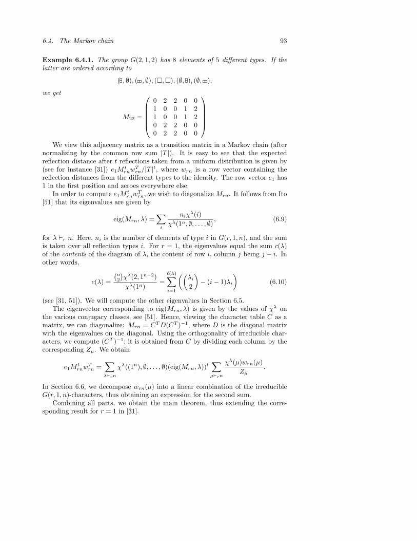
6.4. The Markov chain 93
Example 6.4.1. The group G(2, 1, 2) has 8 elements of 5 different types. If thelatter are ordered according to
( , ∅), ( , ∅), (¤, ¤), (∅, ), (∅, ),
we get
M22 =
0 2 2 0 01 0 0 1 21 0 0 1 20 2 2 0 00 2 2 0 0
We view this adjacency matrix as a transition matrix in a Markov chain (afternormalizing by the common row sum |T |). It is easy to see that the expectedreflection distance after t reflections taken from a uniform distribution is given by(see for instance [31]) e1M
trnwT
rn/|T |t, where wrn is a row vector containing thereflection distances from the different types to the identity. The row vector e1 has1 in the first position and zeroes everywhere else.
In order to compute e1MtrnwT
rn, we wish to diagonalize Mrn. It follows from Ito[51] that its eigenvalues are given by
eig(Mrn, λ) =∑
i
niχλ(i)
χλ(1n, ∅, . . . , ∅) , (6.9)
for λ `r n. Here, ni is the number of elements of type i in G(r, 1, n), and the sumis taken over all reflection types i. For r = 1, the eigenvalues equal the sum c(λ)of the contents of the diagram of λ, the content of row i, column j being j − i. Inother words,
c(λ) =
(n2
)χλ(2, 1n−2)χλ(1n)
=`(λ)∑
i=1
((λi
2
)− (i− 1)λi
)(6.10)
(see [31, 51]). We will compute the other eigenvalues in Section 6.5.The eigenvector corresponding to eig(Mrn, λ) is given by the values of χλ on
the various conjugacy classes, see [51]. Hence, viewing the character table C as amatrix, we can diagonalize: Mrn = CT D(CT )−1, where D is the diagonal matrixwith the eigenvalues on the diagonal. Using the orthogonality of irreducible char-acters, we compute (CT )−1; it is obtained from C by dividing each column by thecorresponding Zµ. We obtain
e1MtrnwT
rn =∑
λ`rn
χλ((1n), ∅, . . . , ∅)(eig(Mrn, λ))t∑
µ`rn
χλ(µ)wrn(µ)Zµ
.
In Section 6.6, we decompose wrn(µ) into a linear combination of the irreducibleG(r, 1, n)-characters, thus obtaining an expression for the second sum.
Combining all parts, we obtain the main theorem, thus extending the corre-sponding result for r = 1 in [31].
94 Paper 6. Expected reflection distance in G(r, 1, n) after t random reflections
Theorem 6.4.2. Assume r, n ∈ N and rn > 1. Then the expected reflectiondistance after t random reflections in G(r, 1, n) is given by
n− 1r
n∑
k=1
1k
+1r
n−1∑p=1
min(p,n−p)∑q=1
apq
(r((
p2
)+
(q−12
)− (n−p−q+2
2
)+ n
)− n
r(n+1
2
)− n
)t
+r − 1
r
n−1∑p=0
n−p∑q=1
bpq
(r((
p2
)+
(q2
)− (n−p−q+1
2
)+ p
)− n
r(n+1
2
)− n
)t
,
where
apq = (−1)n−p−q+1 (p− q + 1)2
(n− q + 1)2(n− p)
(n
p
)(n− p− 1
q − 1
)
and
bpq =(−1)n−p−q+1
n− p
(n
p
)(n− p− 1
q − 1
).
The proof of this theorem is postponed until Section 6.7, since it uses the ma-terial derived in the following two sections.
Example 6.4.3. Returning to the case n = r = 2, M22 diagonalizes as
1 1 2 1 11 −1 0 1 −11 1 0 −1 −11 1 −2 1 11 −1 0 −1 1
4 0 0 0 00 0 0 0 00 0 0 0 00 0 0 0 00 0 0 0 −4
18
1 2 2 1 21 −2 2 1 −22 0 0 −2 01 2 −2 1 −21 −2 −2 1 2
.
We recognize the leftmost matrix in this expression; it is the transpose of the char-acter table of G(2, 1, 2).
Plugging n = r = 2 into Theorem 6.4.2, we get (for t > 0)
2− 34
+12
(−1)2
0t +12
(12· (−1)t − 1
2· 0t − 2 · 0t
)=
54
+(−1)t
4.
The asymptotics are now fairly easy to deal with. For r = 1, 2 we have adependence on the parity of t reflecting the bipartite nature of Grn. For larger r,Grn is no longer bipartite, and this behaviour disappears.
Corollary 6.4.4. As t goes to infinity, the expected reflection distance in G(r, 1, n)approaches
n− 1r
n∑
k=1
1k
+ δ,
6.5. The eigenvalues of the adjacency matrices 95
where
δ =
(−1)n−1
n(n−1) if r = 1 and t is even,(−1)n
n(n−1) if r = 1 and t is odd,(−1)n
2n if r = 2 and t is even,(−1)n+1
2n if r = 2 and t is odd,
0 if r ≥ 3.
Proof. The case r = 1 was carried out in [31], so suppose r ≥ 2. Consider theexpressions inside the large brackets preceded by apq and bpq in Theorem 6.4.2; callthem B1 and B2, respectively. It is easily checked that |B1| < 1 for all p, q. It isequally simple to verify that |B2| < 1 unless p = 0, q = 1, r = 2 in which case wehave B2 = −1. Noting that b01 = (−1)n/n proves the corollary.
6.5 The eigenvalues of the adjacency matrices
To compute the eigenvalues of Mrn, we use the following G(r, 1, n)-version of theMurnaghan-Nakayama formula which can be found in Ariki and Koike [1].
Theorem 6.5.1 ([1]). For fixed i and j, let µij be the jth part of µi in µ =
(µ1, . . . , µr), and let ζ be a primitive rth root of unity in C. Then
χλ(µ) =r∑
p=1
∑
|Γ|=µij
(−1)ht(Γ)ζ(i−1)(p−1)χ(λ1,...,λp−Γ,...,λr)(µ− µij),
where the second sum runs over all rim hooks Γ of size µij in λp and ht(Γ) is one
less than the number of rows in Γ.
From (6.9), it follows that the eigenvalue corresponding to λ `r n is
r(n2
)χλ((2, 1n−2), ∅, . . . , ∅)χλ(1n, ∅, . . . , ∅) +
r∑
i=2
nχλ(1n−1, ∅, . . . , ∅, 1, ∅, . . . , ∅)χλ(1n, ∅, . . . , ∅) , (6.11)
where, in the second sum, the ith argument of χλ is 1.We thus need to compute some entries in the character table of G(r, 1, n).
96 Paper 6. Expected reflection distance in G(r, 1, n) after t random reflections
Lemma 6.5.2. For any λ = (λ1, . . . , λr) `r n, we have
χλ(1n, ∅, . . . , ∅) =(
n
|λ1|, . . . , |λr|) r∏
k=1
χλk
(1|λk|),
χλ((2, 1n−2), ∅, . . . , ∅) =r∑
p=1
(n− 2
|λ1|, . . . , |λp| − 2, . . . , |λr|)
χλp
(2, 1|λp|−2)
∏
k 6=p
χλk
(1|λk|)
and
χλ(1n−1, ∅, . . . , ∅, 1, ∅, . . . , ∅) =r∑
p=1
(n− 1
|λ1|, . . . , |λp| − 1, . . . , |λr|)
ζ(i−1)(p−1)r∏
k=1
χλk
(1|λk|).
(In the last equation, the ith argument of χλ is 1.)
Proof. For µ = (1n, ∅, . . . , ∅), the Murnaghan-Nakayama rule becomes
χλ(1n, ∅, . . . , ∅) =r∑
p=1
∑
χ(λ1,...,λp−,...,λr)(1n−1, ∅, . . . , ∅),
where the inner sum runs over all outer squares of λp. Thus, the character equalsthe number of ways to remove one outer square at a time from the Ferrers’ diagramsof λ. This number is
(n
|λ1|,...,|λr|) ∏r
k=1 χλk
(1|λk|), since χλk
(1|λk|) is the number of
ways to remove one outer square at a time from λk.The two other equations follow similarly. When µ = ((2, 1n−2), ∅, . . . , ∅), we
first remove a rim hook of size 2 from some λp. For µ = (1n−1, ∅, . . . , ∅, 1, ∅, . . . , ∅),we start by removing the square corresponding to µj .
We are now ready to compute the eigenvalues.
Theorem 6.5.3. Let λ = (λ1, . . . , λr) `r n. The eigenvalue of Mrn correspondingto λ is given by
eig(Mrn, λ) = r
r∑p=1
c(λp) + r|λ1| − n.
6.6. Decomposing the distance function 97
Proof. Combining equation (6.11) and Lemma 6.5.2, the eigenvalue becomes
r
r∑p=1
(|λp|2
)χλp
(2, 1|λp|−2)
χλp(1|λp|)+
r∑p=1
|λp|r∑
j=2
ζ(j−1)(p−1).
But(|λp|
2
)χλp
(2, 1|λp|−2)
χλp(1|λp|)= eig(M1|λp|, λp) = c(λp),
andr∑
j=2
ζ(j−1)(p−1) =r∑
j=1
ζ(j−1)(p−1) − 1 =
r − 1 if p = 1,−1 otherwise.
6.6 Decomposing the distance function
Recall from (6.6) the distance function wrn in the reflection graph of G(r, 1, n).Being a class function, it can be written as a linear combination of the irreducibleG(r, 1, n)-characters. In this section, we will make this decomposition explicit usingthe material reviewed in Section 6.3. In [31], the symmetric group case (r = 1) wassettled using a similar approach. However, the fact that xi 6= xi for larger r callsfor greater care.
Before stating the main theorem we need some preliminary results.
Proposition 6.6.1. The complete symmetric functions satisfy
r∏
i=1
∑
n≥0
hn(xi) =
∑
n≥0
hn(x1)
r
.
Proof. Throughout the proof, lower case Greek letters with or without superscripts,such as µ and µi, will denote ordinary integer partitions.
First, we manipulate the left hand side a little to obtain
r∏
i=1
∑
n≥0
hn(xi) =r∏
i=1
∑µ
pµ(xi)zµ
=∑
(µ1,...,µr)
pµ1(x1) . . . pµr (xr)zµ1 . . . zµr
.

98 Paper 6. Expected reflection distance in G(r, 1, n) after t random reflections
Turning to the right hand side, using (6.7), we get∑
n≥0
hn(x1)
r
=
(∑µ
pµ(x1)zµ
)r
=
(∑µ
pµ1(x1) . . . pµ`(µ)(x1)zµ
)r
=
∑
µ
1zµ
`(µ)∏
i=1
pµi(x1) + · · ·+ pµi
(xr)r
r
=∑
(µ1,...,µr)
1zµ1 . . . zµrr`(µ1)+···+`(µr)
r∏
j=1
`(µj)∏
i=1
(pµji(x1) + · · ·+ pµj
i(xr)).
For appropriate coefficients Kµ1,...,µr , this expression can be written as∑
(µ1,...,µr)
Kµ1,...,µrpµ1(x1) . . . pµr (xr).
Fix λ1, . . . , λr. We must show that Kλ1,...,λr = (zλ1 . . . zλr )−1.Consider the last expression for the right hand side above. For a term indexed
by (µ1, . . . , µr), let f ji be the number of parts that equal i in µj . Similarly, let ej
i
be the number of parts that equal i in λj and put Ni =∑
j eji . Clearly, the only
terms that contribute to Kλ1,...,λr are those for which∑
j f ji = Ni for all i. Below,
the sums are over all such µ1, . . . , µr (so that, in particular, `(λ1) + · · · + `(λr) =`(µ1) + · · ·+ `(µr)). We get
Kλ1,...,λr =1
r`(λ1)+···+`(λr)
∑
(µ1,...,µr)
1zµ1 . . . zµr
∏
i≥1
(Ni
e1i , . . . , e
ri
)
=1
r`(λ1)+···+`(λr)
∑
(µ1,...,µr)
∏rk=1(
∏j ek
j !)
zλ1 . . . zλr
∏rk=1(
∏j fk
j !)
∏
i≥1
(Ni
e1i , . . . , e
ri
)
=1
r`(λ1)+···+`(λr)zλ1 . . . zλr
∑
(µ1,...,µr)
∏
i≥1
(Ni
f1i , . . . , fr
i
).
To simplify this sum, consider the following situation: we have r boxes of distin-guishable balls, the ith box containing Ni balls, and we wish to paint the ballsusing (at most) r colours. Of course, colouring the balls one by one, this can bedone in r
PNi = r`(λ1)+···+`(λr) ways. Another way to colour the balls is this: first
choose (µ1, . . . , µr) `r n with∑
j f ji = Ni for all i. In box i, there will be f j
i ballswith colour j; this box can be coloured in
(Ni
f1i ,...,fr
i
)ways. Thus,
Kλ1,...,λr =1
r`(λ1)+···+`(λr)zλ1 . . . zλr
r`(λ1)+···+`(λr) =1
zλ1 . . . zλr
,
as desired.

6.6. Decomposing the distance function 99
Let L ∈ R(r) be the function λ 7→ `(λ1). Sometimes, by abuse of notation, wewill let L denote its restriction to Rn(r).
Lemma 6.6.2. We have
ch(L) =1r
∑
n≥1
1n
pn(x1)r∏
i=1
∑
m≥0
hm(xi)
1r
.
Proof. Again, in this proof symbols such as µ and µi will denote ordinary integerpartitions.
Letting the first t y-variables equal one and the rest be zero in [70, 7.20] yields
∑µ
pµ
zµt`(µ) = exp
∑
n≥1
t
npn
.
Hence, letting ti be independent indeterminates,
r∏
i=1
∑µ
pµ(xi)zµ
t`(µ)i = exp
r∑
i=1
∑
n≥1
tin
pn(xi)
.
Differentiating with respect to t1, we obtain
∑µ
pµ(x1)zµ
`(µ)t`(µ)−11
r∏
i=2
∑ν
pν(xi)zν
t`(ν)i =
∑
n≥1
pn(x1)n
exp
r∑
i=1
∑
m≥1
tim
pm(xi)
,
which, after putting all ti = 1r , becomes
r∑
(µ1,...,µr)
pµ1(x1) . . . pµr (xr)zµ1 . . . zµrr`(µ1)+···+`(µr)
`(µ1) =∑
n≥1
pn(x1)n
exp
1
r
r∑
i=1
∑
m≥1
pm(xi)m
.
Now, the left hand side is in fact rch(L). The fact that exp(∑
m≥1pm
m
)=∑
m≥0 hm concludes the proof.
We are now in position to state and prove the main result of this section.
Theorem 6.6.3. For all λ `r n, L(λ) =∑
µ`rn cµχµ(λ), where
cµ =
∑nk=1
1rk if µ1 = (n),
(−1)n−p−q p−q+1r(n−q+1)(n−p) if µ1 = (p, q, 1n−p−q),
(−1)n−p−q
r(n−p) if µ1 = (p) and µi = (q, 1n−p−q) for some i,
0 otherwise.
100 Paper 6. Expected reflection distance in G(r, 1, n) after t random reflections
Proof. Passing to Λn(r), we want to compute the coefficients cµ in the expressionchn(L) =
∑µ`rn cµSµ.
Combining Lemma 6.6.2 and Proposition 6.6.1 yields
ch(L) =1r
∑
n≥1
1n
pn(x1)∑
m≥0
hm(x1),
which, with the aid of (6.8), becomes
ch(L) =1r
∑
n≥1
1n
r∑
i=1
pn(xi)∑
m≥0
hm(x1).
Now, define coefficients ciµ by writing
∑
m≥0
hm(x1)∑
n≥1
1n
pn(xi) =∑
n
∑
µ`rn
ciµSµ,
so that rcµ =∑r
i=1 ciµ. For the rest of this proof, we let µ `r n be fixed.
First, we consider the case i = 1. Using [70, 7.72], it is not difficult to show that
c1µ =
∑nk=1
1k if µ1 = (n),
(−1)n−p−q p−q+1(n−q+1)(n−p) if µ1 = (p, q, 1n−p−q),
0 otherwise;
see the proof of [31, Theorem 3] for the details.Now, pick i > 1. It is well-known that
pn =n∑
q=1
(−1)n−qs(q,1n−q).
Hence, recalling that sm = hm, we obtain
ciµ =
(−1)n−p−q
n−p if µ1 = (p) and µi = (q, 1n−p−q),0 otherwise.
The result follows.
What we really need is the decomposition of the distance function wrn, not L.It is now easily obtained.
Corollary 6.6.4. For all λ `r n, wrn(λ) =∑
µ`rn dµχµ(λ), where
dµ =
n−∑n
k=11rk if µ1 = (n),
−cµ otherwise.
Here, cµ is as in Theorem 6.6.3.
Proof. We know that wrn = nχtriv − L, where χtriv is the trivial character. Sincethe trivial character is indexed by (n, ∅, . . . , ∅), the result follows.
6.7. Proof of Theorem 6.4.2 101
6.7 Proof of Theorem 6.4.2
We now turn to the proof of our main theorem. We have already shown that theexpected reflection distance after t random reflections is given by
∑
λ`rn
χλ(1n, ∅, . . . , ∅)(
eig(Mrn, λ)|T |
)t ∑
µ`rn
χλ(µ)wrn(µ)Zµ
=∑
λ`rn
χλ(1n, ∅, . . . , ∅)(
eig(Mrn, λ)|T |
)t
〈χλ, wrn〉.
If we decompose wrn(µ) =∑
λ`rn dλχλ(µ) and use that the number of reflectionsis |T | = r
(n+1
2
)− n, we obtain
∑
λ`rn
dλχλ(1n, ∅, . . . , ∅)(
eig(Mrn, λ)r(n+1
2
)− n
)t
.
The coefficients dλ are zero for most λ, the exceptions being λ1 = (n), λ1 =(p, q, 1n−p−q) and λ = (p, ∅, . . . , ∅, (q, 1n−p−q), ∅, . . . , ∅).
If λ1 = (n), we have dλ = n − ∑nk=1
1rk , χλ(1n, ∅, . . . , ∅) = 1 (since χλ is the
trivial character) and eig(Mrn, λ) = r(n2
)+ (r − 1)n = r
(n+1
2
)− n, so we get
dλχλ(1n, ∅, . . . , ∅)(
eig(Mrn, λ)r(n+1
2
)− n
)t
= n−n∑
k=1
1rk
.
Similarily, if λ1 = (p, q, 1n−p−q), we obtain dλ = (−1)n−p−q+1 p−q+1r(n−q+1)(n−p) ,
χλ(1n, ∅, . . . , ∅) =n!(p− q + 1)
(q − 1)!(n− p− q)!(n− p)(n− q + 1)p!
=(p− q + 1)(n− q + 1)
(n− p− 1
q − 1
)(n
p
)
and eig(Mrn, λ) = rc(p, q, 1n−p−q) + (r − 1)n.Finally, if λ1 = (p) and λi = (q, 1n−p−q), we have dλ = (−1)n−p−q+1
r(n−p) ,
χλ(1n, ∅, . . . , ∅) =(
n
p
)χ(p)(1p)χ(q,1n−p−q)(1n−p) =
(n
p
)(n− p− 1
q − 1
)
and
eig(Mrn, λ) = r
((p
2
)+
(q
2
)−
(n− p− q + 1
2
)+ p
)− n.
Putting it all together yields the theorem.

102
Bibliography
[1] S. Ariki and K. Koike, A Hecke algebra of (Z/rZ) oSn and construction of itsirreducible representations, Adv. Math. 106 (1994), 216–243.
[2] E. Babson, A. Bjorner, S. Linusson, J. Shareshian and V. Welker, Complexesof not i-connected graphs, Topology 38 (1999), 271–299.
[3] E. Babson and D. Kozlov, Group actions on posets, preprint, 2001.
[4] V. Bafna and P. Pevzner, Genome rearrangements and sorting by reversals,SIAM J. Comput. 25 (1996), 272–289.
[5] G. Bourque and P. Pevzner, Genome-scale evolution: Reconstructing geneorders in the ancestral species, Genome Research 12 (2002), 26–36.
[6] A. Bjorner, Shellable and Cohen-Macaulay partially ordered sets, Trans. Amer.Math. Soc. 1 (1980), 159–183.
[7] A. Bjorner, Orderings of Coxeter groups, in “Combinatorics and algebra (Boul-der, Colo. 1983)”, 175–195, Contemp. Math. 34, Amer. Math. Soc., Provi-dence, R. I., 1984.
[8] A. Bjorner, Posets, regular CW-complexes and Bruhat order, European J.Combin. 5 (1984), 7–16.
[9] A. Bjorner, Subspace arrangements, First European Congress of Math., Paris,1992 (A. Joseph et al., eds.), 321–370, Progr. Math 119, Birkhauser, Basel,1994.
[10] A. Bjorner, Topological methods, in Handbook of Combinatorics (R. Graham,M. Grotschel and L. Lovasz, eds.), North-Holland, 1995, 1819–1872.
[11] A. Bjorner, personal communication, 2001.
[12] A. Bjorner and F. Brenti, Combinatorics of Coxeter groups, Graduate Textsin Mathematics, Springer Verlag, to appear.
103
104 Bibliography
[13] A. Bjorner, P. H. Edelman and G. M. Ziegler, Hyperplane arrangements witha lattice of regions, Discrete Comput. Geom. 5 (1990), 263–288.
[14] A. Bjorner and B. Sagan, Subspace arrangements of type Bn and Dn, J. Al-gebraic Combin. 5 (1996), 291–314.
[15] A. Bjorner and M. Wachs, Bruhat order of Coxeter groups and shellability,Adv. in Math. 43 (1982), 87–100.
[16] A. Bjorner and M. Wachs, Shellable nonpure complexes and posets I, Trans.Amer. Math. Soc. 4 (1996), 1299–1327.
[17] A. Bjorner and M. Wachs, Shellable nonpure complexes and posets II, Trans.Amer. Math. Soc. 10 (1997), 3945–3975.
[18] A. Bjorner and V. Welker, Complexes of directed graphs, SIAM J. DiscreteMath. 12 (1999), 413–424.
[19] G. E. Bredon Introduction to compact transformation groups, Academic Press,1972.
[20] F. Brenti, Kazhdan-Lusztig and R-polynomials from a combinatorial point ofview, Selected papers in honour of Adriano Garsia (Taormina, 1994), DiscreteMath. 193 (1998), 93–116.
[21] A. Caprara, On the tightness of the alternating-cycle lower bound for sortingby reversals, J. Comb. Optim. 3 (1999), 149–182.
[22] M. Chari, On discrete Morse functions and combinatorial decompositions, Dis-crete Math. 217 (2000), 101-113.
[23] V. Deodhar, A note on the subgroups generated by reflections in Coxetergroups, Arch. Math. (Basel) 53 (1989), 543–546.
[24] X. Dong, Topology of bounded-degree graph complexes, J. Algebra 262 (2003),287–312.
[25] A. Duval, Free resolutions of simplicial posets, J. Algebra 188 (1997), 363-399.
[26] T. A. Dowling, A class of geometric lattices based on finite groups, J. Combin.Theory Ser. B 14 (1973), 61–86.
[27] M. Dyer, Reflection subgroups of Coxeter systems, J. Algebra 135 (1990),57–73.
[28] M. Dyer, On the “Bruhat graph” of a Coxeter system, Compositio Math. 78(1991), 185–191.
[29] M. Dyer, personal communication, 2003.
Bibliography 105
[30] N. Eriksen, Approximating the expected number of inversions given the num-ber of breakpoints, Algorithms in Bioinformatics, Proceedings of WABI 2002,LNCS 2452 (2002), 316–330.
[31] N. Eriksen and A. Hultman, Estimating the expected reversal distance after afixed number of reversals, Adv. in Appl. Math., to appear.
[32] N. Eriksen and A. Hultman, Expected reflection distance in G(r, 1, n) after afixed number of reflections, preprint 2002.
[33] M. Erne and J. Reinhold, Intervals in lattices of quasiorders, Order 12 (1995),375–403.
[34] R. Forman, Morse theory for cell complexes, Adv. in Math. 134 (1998), 90–145.
[35] A. M. Garsia and M. Haiman, A graded representation model for Macdonald’spolynomials, Proc. Nat. Acad. Sci. U.S.A. 90 (1993), 3607–3610.
[36] A. Garsia and D. Stanton, Group actions of Stanley-Reisner rings and invari-ants of permutation groups, Adv. in Math. 51 (1984), 107–201.
[37] D. Gebhard and B. Sagan, Sinks in acyclic orientations of graphs, J. Combin.Theory Ser. B 80 (2000), 130–146.
[38] M. Goresky, Kazdhan-Lusztig polynomials for classical groups, NortheasternUniversity, Boston, preprint 1981.
[39] M. Goresky and R. D. MacPherson, Stratified Morse theory, Ergebnisse derMathematik und ihrer Grenzgebiete, vol. 14, Springer-Verlag, Berlin/Heidel-berg/New York, 1988.
[40] C. Greene and T. Zaslavsky, On the interpretation of Whitney numbersthrough arrangements of hyperplanes, zonotopes, non-Radon partitions andorientations of graphs, Trans. Amer. Math. Soc. 280 (1983), 97–126.
[41] M. Haiman, Hilbert schemes, polygraphs, and the Macdonald positivity con-jecture, J. Amer. Math. Soc. 14 (2001), 941–1006.
[42] M. Haiman, Macdonald polynomials and geometry, in New perspectives inalgebraic combinatorics (L. J. Billera et al., eds.), 207–254, Cambridge Univ.Press, 1999.
[43] M. Haiman, personal communication, 2001.
[44] S. Hannenhalli, P. Pevzner, Transforming cabbage into turnip (polynomialalgorithm for sorting signed permutations with reversals), Proceedings of the27th Annual ACM Symposium on the Theory of Computing (1995), 178–189.
106 Bibliography
[45] P. Hersh, Lexicographic shellability for balanced complexes, J. Algebraic Com-bin. 17 (2003), 225–254.
[46] A. Hultman, Quotient complexes and lexicographic shellability, J. AlgebraicCombin. 16 (2002), 83–96.
[47] A. Hultman, Polygraph arrangements, European J. Combin. 23 (2002), 937–948.
[48] A. Hultman, Directed subgraph complexes, preprint 2003.
[49] A. Hultman, Bruhat intervals of length 4 in Weyl groups, J. Combin. Theory,Ser. A 102 (2003), 163–178.
[50] J. E. Humphreys, Reflection groups and Coxeter groups, Cambridge Univ.Press, 1990.
[51] N. Ito, The spectrum of a conjugacy class graph of a finite group, Math. J.Okayama Univ. 26 (1984), 1–10.
[52] J. Jantzen, Moduln mit einem hochsten Gewicht, Lecture Notes in Math., vol.750, Springer-Verlag, Berlin, 1979.
[53] J. Jonsson, On the topology of simplicial complexes related to 3-connected andHamiltonian graphs, preprint 2002.
[54] D. Kozlov, General lexicographic shellability and orbit arrangements, Ann.Comb. 1 (1997), 67–90.
[55] D. Kozlov, Complexes of directed trees, J. Combin. Theory Ser. A 88 (1999),112–122.
[56] D. Kozlov, Collapsibility of ∆(Πn)/Sn and some related CW complexes, Proc.Amer. Math. Soc. 128 (2000), 2253–2259.
[57] D. Kozlov, Rational homology of spaces of complex monic polynomials withmultiple roots, Math. CO/0111167.
[58] S. Linusson and J. Shareshian, Complexes of t-colorable graphs, SIAM J. Dis-crete Math. 16 (2003), 371–389.
[59] I. G. Macdonald, A new class of symmetric functions, Actes du 20e SeminaireLotharingien, vol. 372/S-20, Publications I.R.M.A., Strasbourg, 1988, 131–171
[60] I. G. MacDonald, Symmetric Functions and Hall Polynomials, second ed.,Oxford University Press, Oxford, 1995.
Bibliography 107
[61] B. M. E. Moret, A. C. Siepel, J. Tang and T. Liu, Inversion medians outper-form breakpoint medians in phylogeny reconstruction from gene-order data,Algorithms in Bioinformatics, Proceedings of WABI 2002, LNCS 2452 (2002),521–536.
[62] J. R. Munkres, Elements of algebraic topology, Addison-Wesley, Menlo Park,1984.
[63] D. Quillen, Homotopy properties of the poset of non-trivial p-subgroups of agroup, Adv. in Math. 28 (1978), 101–128.
[64] V. Reiner, Quotients of Coxeter complexes and P-partitions, Memoirs. Amer.Math. Soc. 95, January 1992.
[65] G.-C. Rota, On the foundations of combinatorial theory. I. Theory of Mobiusfunctions, Z. Warsch. Verw. Gebiete 2 (1964) 340–368.
[66] G. C. Shephard, Regular complex polytopes, Proc. London Math. Soc. 2(1952), 82–97.
[67] G. C. Shephard and J. A. Todd, Finite unitary reflection groups, Canadian J.Math. 6 (1954), 274–304.
[68] R. P. Stanley, f -vectors and h-vectors of simplicial posets, J. Pure Appl. Al-gebra 71 (1991), 319–331.
[69] R. P. Stanley, Enumerative Combinatorics, vol. 1, Cambridge Univ. Press 1997.
[70] R. P. Stanley,Enumerative Combinatorics, vol. 2, Cambridge Univ. Press 1999.
[71] J. R. Stembridge, COXETER ver. 2.1, Maple package, 1998.
[72] J. R. Stembridge, COXETER ver. 2.3, Maple package, 2002, see web pagehttp://www.math.lsa.umich.edu/∼jrs/maple.html.
[73] J. R. Stembridge, POSETS ver. 2.2, Maple package, 2002, see web pagehttp://www.math.lsa.umich.edu/∼jrs/maple.html.
[74] V. Turchin, Homologies of complexes of biconnected graphs, Russian Math.Surveys 52 (1997), 426–427.
[75] M. Wachs, Topology of matching, chessboard and general bounded degreegraph complexes, Algebra Universalis, Special issue in memory of Gian-CarloRota, to appear.
[76] L.-S. Wang, Estimating true evolutionary distances between genomes, Proceed-ings of STOC (2001), 637–646.

108 Bibliography
[77] V. Welker, The topology of posets and orbit posets, in Coding theory, designtheory, group theory (Burlington, VT, 1990), Wiley-Intersci. Publ., Wiley, NewYork, 1993, 283–289.
[78] T. Zaslavsky, Signed graphs, Discrete Appl. Math. 4 (1982), 47–74.
[79] G. M. Ziegler and R. T. Zivaljevic, Homotopy types of subspace arrangementsvia diagrams of spaces, Math. Ann. 295 (1993), 527–548.