Embed Size (px)
Citation preview
COMBINATORIAL DIOPHANTINE EQUATIONS AND AREFINEMENT OF A THEOREM ON SEPARATED VARIABLES
EQUATIONS
YURI F. BILU, CLEMENS FUCHS, FLORIAN LUCA, AND AKOS PINTER
Abstract. We look at Diophantine equations arising from equating classical countingfunctions such as perfect powers, binomial coefficients and Stirling numbers of the firstand second kind. The proofs of the finiteness statements that we give use a varietyof methods from modern number theory, such as effective and ineffective tools fromDiophantine approximation. As a tool for one part of the statements we establish atheoretical result that gives a more precise description on the structure of the solutionset in the theorem, due to Bilu and Tichy, on Diophantine equations with separatevariables in the case when infinitely many solutions exist.
1. Introduction and results
Elementary counting functions appear in several areas of mathematics. The study oftheir arithmetical properties has a long history. In this paper, we are interested in studyingthe Diophantine equations which arise when two such counting functions are set to equaleach other. The combinatorial background to this question is quite obvious. The countingfunctions that we are studying are the following:
nk – Perfect powers: giving the number of maps from a set with k elements to a setof n elements, or the number of integer points in a k-dimensional cube with sidelength n and having one of its corners at the origin and the sides parallel to thecoordinate axes;(
nk
)– Binomial coefficients: giving the number of subsets with k elements of a set of n
elements;Snk – Stirling numbers of the second kind: giving the number of partitions in k nonempty
disjoint subsets of a set of n elements;snk – Stirling numbers of the first kind: giving the number of permutations with k dis-
joint cycles of a set with n elements.
For the proofs of our main results, we will use a variety of methods from modern numbertheory, ranging from effective tools provided by Baker’s theory of lower bounds for nonzero
2010 Mathematics Subject Classification. Primary 11D41, 11D61; Secondary 05A19, 11B65, 11B73, 14G05.Key words and phrases: Diophantine equations, counting functions, Stirling numbers, effective and inef-fective methods, Diophantine equations with separate variables.
Research of F. L. was supported in part by Grants SEP-CONACyT 79865, PAPIIT 100508. Researchof A. P. was supported in part by the Hungarian Academy of Sciences, OTKA grants T67580, K75566,K100339, NK101680, NK104208 and the Project TAMOP 4.2.1./B-09/1/KONV-2010-0007 implementedthrough the New Hungary Development Plan co-financed by the European Social Fund and the EuropeanRegional Development Fund. Furthermore, Yu.F. B. and F. L. were supported in part by the joint projectFrance–Mexico 121469 “Linear recurrences, arithmetic functions and additive combinatorics”, and F. L.and A. P. were supported in part by the joint project Hungary-Mexico J.010.106 “Diophantine Equationsand Applications in Cryptography”. Part of this research was done while C. F. visited the Institute ofMathematics of the University of Debrecen in November 2009 and another part while F. L. visited theDepartment of Mathematics at ETH Zurich in March 2010.
1
2 YU.F. BILU, C. FUCHS , F. LUCA, AND A. PINTER
linear forms in logarithms in algebraic numbers, to ineffective methods such as the recentapplications of the subspace theorem a la Corvaja and Zannier, as well as the finitenesstheorem on separated variables equations from [8], see Theorem BT in Section 2.
We mention that in the course of applying Theorem BT the question arose whether onecan get a more precise result on the structure of the solution set of such equations withseparate variables in case that infinitely many solutions exist. This was the point whenthe first author joined in this project and contributed this general theoretical statement.A complete treatment, even in the more general case of rational solutions with boundeddenominator, is given in Section 2 below. Using this new result, which is Theorem 4, onecan rule out several cases immediately making the treatment of our equations via theTheorem BT much simpler. Clearly, this statement will be useful also for future concreteapplications of this method.
Many arithmetical properties of the counting functions introduced above are well-knownand we shall make use of some of these properties. All these numbers satisfy recurrencerelations. For example, if we set S0
0 = 1 and Sn0 = 0 for all n ≥ 1, then the recurrenceSn+1k = Snk−1 + kSnk holds for all n, k ≥ 0. Furthermore, if we set s0
0 = 1 and sn0 = 0 for
all n ≥ 1, then the recurrence sn+1k = snk−1 − nsnk holds for all n, k ≥ 0.
We also have
(1) Sna =1
a!
{an −
(a
1
)(a− 1)n + . . .+ (−1)a−1
(a
a− 1
)1n},
and
(2) Snn−a =
(n
a+ 1
)Sa+1
1 + . . .+
(n
2a
)S2aa ,
where Snk are the associated Stirling numbers of the second kind. These associated Stirling
numbers also have a combinatorial meaning, namely, Snk counts the number of partitionsof a set with n elements into k disjoint parts each having at least 2 elements. While wealso have a similar representation as (2) for the analogous Stirling numbers of the firstkind, namely
(3) snn−a =
(n
a+ 1
)sa+1
1 + . . .+
(n
2a
)s2aa ,
where snk are certain associated Stirling numbers of the first kind, there is no knownformula analogous to (1) in the literature for Stirling numbers of the first kind. From theabove identities, we see that for varying n and fixed a the function Sna is an exponentialpolynomial, or the nth term of a linearly recurrent sequence whose roots are all simpleand given by {1, . . . , a}, whereas the functions Snn−a, s
nn−a are polynomials of degree 2a in
n.In this paper, we study the Diophantine equations resulting from when two such count-
ing functions are set to equal each other. Some of the resulting Diophantine equations areeasy, such as xa = yb for given positive integers a and b where the unknowns are integersx and y. Other equations of this type have already been studied in the literature such as(
x
a
)= yb, or
(x
a
)=
(y
b
),
again for given integers a > 1 and b > 1 with integer solutions (x, y). For the first equation,the complete list of solutions, even with variable a > 1 and b > 1, appears in [21], whichis based on results from [3] and [15]. Assuming that x ≥ 2a, all solutions have a = b = 2except for (x, a, b, y) = (50, 3, 2, 140). For fixed a > b > 1, the second equation has only

COMBINATORIAL DIOPHANTINE EQUATIONS WITH SEPARATED VARIABLES 3
finitely many positive integer solutions (x, y) (see [5]). For a list of solutions of the secondequation for various small values of the parameters a and b, see [11], [30] and [31].
In a similar vein, effective upper bounds for the maximum of positive integers x, y andz > 1 in the equations
Sxx−a = byz, or sxx−a = byz,
where a and b are given positive integers, appear in [10]. All such equations have onlyfinitely many solutions except when z = 2 and a ∈ {1, 3}; in these exceptional cases theequations lead to Pell equations which may have infinitely many solutions. In the samepaper [10], it was shown that the equation
Sxa = byz
with fixed integers a ≥ 2 and b ≥ 1, where x, y, z > 1 are positive integer variables,implies that z is bounded by an effective constant depending only on a and b. The factthat there are only finitely many possibilities for x and y as well was shown in [22].
In [25], it was proved that if positive integers x and y are such that
(4) Sxa = Syb
for some fixed positive integers a and b, then the maximum of x and y is bounded by aneffective constant depending on a and b. It is conjectured in [17] that all the non-trivialsolutions of equation (4) (here, by non-trivial we mean x ≥ a > 1 and y ≥ b > 1) are
S65 = S5
2 = 15 and S9190 = S15
2 = 4095.
This conjecture is known to be true for max{a, b} ≤ 100.Here, we look at several of the remaining cases and we prove finiteness statements. For
small values of the parameters, we give effective results. However, our general statementsare ineffective. The case of snn−k falls somewhat outside of our treatment because we couldnot deduce the desired finiteness result for this counting function out of the arithmeticalinformation available to us on these numbers. The motivation for such equations is quiteobvious. Observe, for example, that the equation Sx2 =
(y2
)can be rewritten as 2x+2 =
(2y − 1)2 + 7, which we recognize as the famous and well-studied Ramanujan-Nagellequation.
The first combinations of equations we are interested in are those in which Sna is involved.Our proof here uses a method introduced by Corvaja and Zannier in [13] which relies onthe Schmidt subspace theorem [28]. This method was already used in [22].
Theorem 1. Let a ≥ 2, b ≥ 2, c 6= 0 and d ≥ 1 be integers. Then the Diophantineequations
(5) Sxa = cyb, Sxa =
(y
b
), Sxa = Syy−d, Sxa = syy−d
each have only finitely many positive integer solutions (x, y).
The next finiteness result deals with the remaining combinations of our classical count-ing functions. Here, the proofs rely on the already mentioned finiteness theorem from [8](in the refined form stated as Theorem 4 below), whose proof in turn rests on results byFried, Schinzel, and a classical result by Siegel.
Theorem 2. Let a and b be positive integers. Then the Diophantine equations
Sxx−a = Syy−b, (a > b > 1),
Sxx−a = syy−b, (a > 1, b > 1),
sxx−a = syy−b, (a > b > 1),
4 YU.F. BILU, C. FUCHS , F. LUCA, AND A. PINTER
Sxx−a =
(y
b
), (a > 1, b > 2),
sxx−a =
(y
b
), (a > 1, b > 2)
each have only finitely positive integer solutions (x, y).
For small values of parameters, we present an effective result whose proof relies on aneffective theorem due to Baker [2] based itself on linear forms in logarithms.
Theorem 3. For fixed a ≥ 2, the Diophantine equation
Sxx−a = Syy−1 = syy−1 =
(y
2
)has only finitely many integer solutions (x, y). Furthermore, they are all effectively comp-utable.
We could not prove the same result as Theorem 3 for the similar equations involvingsxx−a instead of Sxx−a. We leave this as an open problem for the reader.
Remark. Using Runge’s method (see, for example, [23], [26] and [33]), it is easy to solvethe equations Sxx−2 =
(y2
)and sxx−2 =
(y2
)in integers x ≥ 3 and y ≥ 2. We detail this
approach for the first equation only, because for the second equation the entire argumentcan be repeated. It is known that
Sxx−2 =1
24x(x− 1)(x− 2)(3x− 5),
and by the transformation u := 3x and v := 9(2y − 1), the first equation leads to thequartic Diophantine equation
u(u− 3)(u− 5)(u− 6) + 81 = u4 − 14u3 + 63a2 − 90a+ 81 = v2.
The polynomial on the left-hand side of the last equation above is monic and of evendegree, so Runge’s method applies. In fact, some straightforward calculations yield thatfor u ≥ 24 we have
(u2 − 7u+ 7)2 < u4 − 14u3 + 63a2 − 90a+ 81 = v2 < (u2 − 7u+ 8)2.
From these inequalities, we deduce easily that all the solutions of the equation Sxx−2 =(y2
)satisfy x < 8. Testing this small range reveals that the only solution is (x, y) = (3, 2). Ina forthcoming paper, we solve some further special cases of the above equations.
2. Separate variables equations with infinitely many solutions
In [8], the first author and Tichy proved Theorem BT below which basically says thatif an equation of the type f(x) = g(y) has infinitely many positive integer solutions x, y,then, up to certain transformations on the space of polynomials, the pair of polynomials(f(X), g(X)) must belong to one of five well-understood families of pairs of polynomialswhich they called standard. Therefore in concrete applications, as for example to treatthe equations from Theorem 2, all one needs to do is to show that the polynomialsunder consideration are not related in the way the Theorem BT asserts to the pairs ofpolynomials belonging to the standard families.
COMBINATORIAL DIOPHANTINE EQUATIONS WITH SEPARATED VARIABLES 5
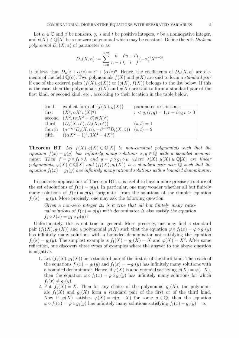
Let α ∈ C and β be nonzero, q, s and t be positive integers, r be a nonnegative integer,and v(X) ∈ Q[X] be a nonzero polynomial which may be constant. Define the nth Dicksonpolynomial Dn(X,α) of parameter α as
Dn(X,α) :=
[n/2]∑i=0
n
n− i
(n− ii
)(−α)iXn−2i.
It follows that Dn(z + α/z) = zn + (α/z)n. Hence, the coefficients of Dn(X,α) are ele-ments of the field Q(α). Two polynomials f(X) and g(X) are said to form a standard pairif one of the ordered pairs (f(X), g(X)) or (g(X), f(X)) belongs to the list below. If thisis the case, then the polynomials f(X) and g(X) are said to form a standard pair of thefirst kind, or second kind, etc., according to their location in the table below.
kind explicit form of {f(X), g(X)} parameter restrictionsfirst (Xq, αXrv(X)q) r < q, (r, q) = 1, r + deg v > 0second (X2, (αX2 + β)v(X)2)third (Ds(X,α
t), Dt(X,αs)) (s, t) = 1
fourth (α−s/2Ds(X,α),−β−t/2Dt(X, β)) (s, t) = 2fifth ((αX2 − 1)3, 3X4 − 4X3) –
Theorem BT. Let f(X), g(X) ∈ Q[X] be non-constant polynomials such that theequation f(x) = g(y) has infinitely many solutions x, y ∈ Q with a bounded denomi-nator. Then f = ϕ ◦ f1 ◦ λ and g = ϕ ◦ g1 ◦ µ where λ(X), µ(X) ∈ Q[X] are linearpolynomials, ϕ(X) ∈ Q[X] and (f1(X), g1(X)) is a standard pair over Q such that theequation f1(x) = g1(y) has infinitely many rational solutions with a bounded denominator.
In concrete applications of Theorem BT, it is useful to have a more precise structure ofthe set of solutions of f(x) = g(y). In particular, one may wonder whether all but finitelymany solutions of f(x) = g(y) “originate” from the solutions of the simpler equationf1(x) = g1(y). More precisely, one may ask the following question:
Given a non-zero integer ∆, is it true that all but finitely many ratio-nal solutions of f(x) = g(y) with denominator ∆ also satisfy the equationf1 ◦ λ(x) = g1 ◦ µ(y)?
Unfortunately, this is not true in general. More precisely, one may find a standardpair (f1(X), g1(X)) and a polynomial ϕ(X) such that the equation ϕ ◦ f1(x) = ϕ ◦ g1(y)has infinitely many solutions with a bounded denominator not satisfying the equationf1(x) = g1(y). The simplest example is f1(X) = g1(X) = X and ϕ(X) = X2. After somereflection, one discovers three types of examples where the answer to the above questionis negative:
1. Let (f1(X), g1(X)) be a standard pair of the first or of the third kind. Then each ofthe equations f1(x) = g1(y) and f1(x) = −g1(y) has infinitely many solutions witha bounded denominator. Hence, if ϕ(X) is a polynomial satisfying ϕ(X) = ϕ(−X),then the equation ϕ ◦ f1(x) = ϕ ◦ g1(y) has infinitely many solutions for whichf1(x) 6= g1(y).
2. Put f1(X) = X. Then for any choice of the polynomial g1(X), the polynomi-als f1(X) and g1(X) form a standard pair of the first or of the third kind.Now if ϕ(X) satisfies ϕ(X) = ϕ(a−X) for some a ∈ Q, then the equationϕ ◦ f1(x) = ϕ ◦ g1(y) has infinitely many solutions satisfying f1(x) + g1(y) = a.
6 YU.F. BILU, C. FUCHS , F. LUCA, AND A. PINTER
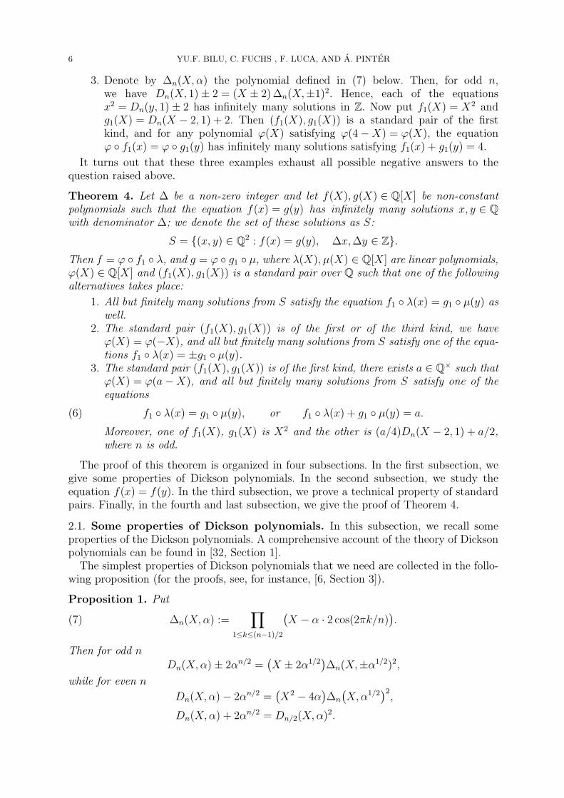
3. Denote by ∆n(X,α) the polynomial defined in (7) below. Then, for odd n,we have Dn(X, 1)± 2 = (X ± 2) ∆n(X,±1)2. Hence, each of the equationsx2 = Dn(y, 1)± 2 has infinitely many solutions in Z. Now put f1(X) = X2 andg1(X) = Dn(X − 2, 1) + 2. Then (f1(X), g1(X)) is a standard pair of the firstkind, and for any polynomial ϕ(X) satisfying ϕ(4−X) = ϕ(X), the equationϕ ◦ f1(x) = ϕ ◦ g1(y) has infinitely many solutions satisfying f1(x) + g1(y) = 4.
It turns out that these three examples exhaust all possible negative answers to thequestion raised above.
Theorem 4. Let ∆ be a non-zero integer and let f(X), g(X) ∈ Q[X] be non-constantpolynomials such that the equation f(x) = g(y) has infinitely many solutions x, y ∈ Qwith denominator ∆; we denote the set of these solutions as S:
S = {(x, y) ∈ Q2 : f(x) = g(y), ∆x,∆y ∈ Z}.Then f = ϕ ◦ f1 ◦ λ, and g = ϕ ◦ g1 ◦ µ, where λ(X), µ(X) ∈ Q[X] are linear polynomials,ϕ(X) ∈ Q[X] and (f1(X), g1(X)) is a standard pair over Q such that one of the followingalternatives takes place:
1. All but finitely many solutions from S satisfy the equation f1 ◦ λ(x) = g1 ◦ µ(y) aswell.
2. The standard pair (f1(X), g1(X)) is of the first or of the third kind, we haveϕ(X) = ϕ(−X), and all but finitely many solutions from S satisfy one of the equa-tions f1 ◦ λ(x) = ±g1 ◦ µ(y).
3. The standard pair (f1(X), g1(X)) is of the first kind, there exists a ∈ Q× such thatϕ(X) = ϕ(a−X), and all but finitely many solutions from S satisfy one of theequations
(6) f1 ◦ λ(x) = g1 ◦ µ(y), or f1 ◦ λ(x) + g1 ◦ µ(y) = a.
Moreover, one of f1(X), g1(X) is X2 and the other is (a/4)Dn(X − 2, 1) + a/2,where n is odd.
The proof of this theorem is organized in four subsections. In the first subsection, wegive some properties of Dickson polynomials. In the second subsection, we study theequation f(x) = f(y). In the third subsection, we prove a technical property of standardpairs. Finally, in the fourth and last subsection, we give the proof of Theorem 4.
2.1. Some properties of Dickson polynomials. In this subsection, we recall someproperties of the Dickson polynomials. A comprehensive account of the theory of Dicksonpolynomials can be found in [32, Section 1].
The simplest properties of Dickson polynomials that we need are collected in the follo-wing proposition (for the proofs, see, for instance, [6, Section 3]).
Proposition 1. Put
(7) ∆n(X,α) :=∏
1≤k≤(n−1)/2
(X − α · 2 cos(2πk/n)
).
Then for odd n
Dn(X,α)± 2αn/2 =(X ± 2α1/2
)∆n(X,±α1/2)2,
while for even n
Dn(X,α)− 2αn/2 =(X2 − 4α
)∆n
(X,α1/2
)2,
Dn(X,α) + 2αn/2 = Dn/2(X,α)2.
COMBINATORIAL DIOPHANTINE EQUATIONS WITH SEPARATED VARIABLES 7
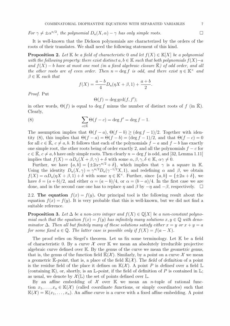
For γ 6= ±αn/2, the polynomial Dn(X,α)− γ has only simple roots. �
It is well-known that the Dickson polynomials are characterized by the orders of theroots of their translates. We shall need the following statement of this kind.
Proposition 2. Let K be a field of characteristic 0 and let f(X) ∈ K[X] be a polynomialwith the following property: there exist distinct a, b ∈ K such that both polynomials f(X)−aand f(X)− b have at most one root (in a fixed algebraic closure K) of odd order, and allthe other roots are of even order. Then n = deg f is odd, and there exist η ∈ K× andβ ∈ K such that
f(X) =a− b
4Dn(ηX + β, 1) +
a+ b
2.
Proof. PutΘ(f) = deg gcd(f, f ′);
in other words, Θ(f) is equal to deg f minus the number of distinct roots of f (in K).Clearly,
(8)∑c∈K
Θ(f − c) = deg f ′ = deg f − 1.
The assumption implies that Θ(f − a), Θ(f − b) ≥ (deg f − 1)/2. Together with iden-tity (8), this implies that Θ(f − a) = Θ(f − b) = (deg f − 1)/2, and that Θ(f − c) = 0for all c ∈ K, c 6= a, b. It follows that each of the polynomials f − a and f − b has exactlyone simple root, the other roots being of order exactly 2, and all the polynomials f − c forc ∈ K, c 6= a, b have only simple roots. Then clearly n = deg f is odd, and [32, Lemma 1.11]implies that f(X) = αDn(X + β, γ) + δ with some α, β, γ, δ ∈ K, αγ 6= 0.
Further, we have {a, b} = {±2αγn/2 + δ}, which implies that γ is a square in K.Using the identity Dn(X, γ) = γn/2Dn(γ−1/2X, 1), and redefining α and β, we obtainf(X) = αDn(ηX + β, 1) + δ with some η ∈ K×. Further, since {a, b} = {±2α + δ}, wehave δ = (a+ b)/2, and either α = (a− b)/4, or α = (b− a)/4. In the first case we aredone, and in the second case one has to replace η and β by −η and −β, respectively. �
2.2. The equation f(x) = f(y). Our principal tool is the following result about theequation f(x) = f(y). It is very probable that this is well-known, but we did not find asuitable reference.
Proposition 3. Let ∆ be a non-zero integer and f(X) ∈ Q[X] be a non-constant polyno-mial such that the equation f(x) = f(y) has infinitely many solutions x, y ∈ Q with deno-minator ∆. Then all but finitely many of these solutions satisfy either x = y or x+ y = afor some fixed a ∈ Q. The latter case is possible only if f(X) = f(a−X).
The proof relies on Siegel’s theorem. Let us fix some terminology. Let K be a fieldof characteristic 0. By a curve X over K we mean an absolutely irreducible projectivealgebraic curve defined over K. By the genus of the curve we mean the geometric genus,that is, the genus of the function field K(X ). Similarly, by a point on a curve X we meana geometric K-point, that is, a place of the field K(X ). The field of definition of a pointis the residue field of the place it defines on K(X ). A point P is defined over a field L(containing K), or, shortly, is an L-point, if the field of definition of P is contained in L;as usual, we denote by X (L) the set of points defined over L.
By an affine embedding of X over K we mean an n-tuple of rational func-tion x1, . . . , xn ∈ K(X ) (called coordinate functions, or simply coordinates) such thatK(X ) = K(x1, . . . , xn). An affine curve is a curve with a fixed affine embedding. A point
8 YU.F. BILU, C. FUCHS , F. LUCA, AND A. PINTER
at infinity of an affine curve is a point which is a pole of at least one of the coordinatefunctions. There are only finitely many points at infinity; all the other points are calledfinite points. Let R be a subring of K; an R-point is a finite point P defined over the quo-tient field of R such that x1(P ), . . . , xn(P ) ∈ R. The set of R-points on an affine curve Xwill be denoted by X (R).
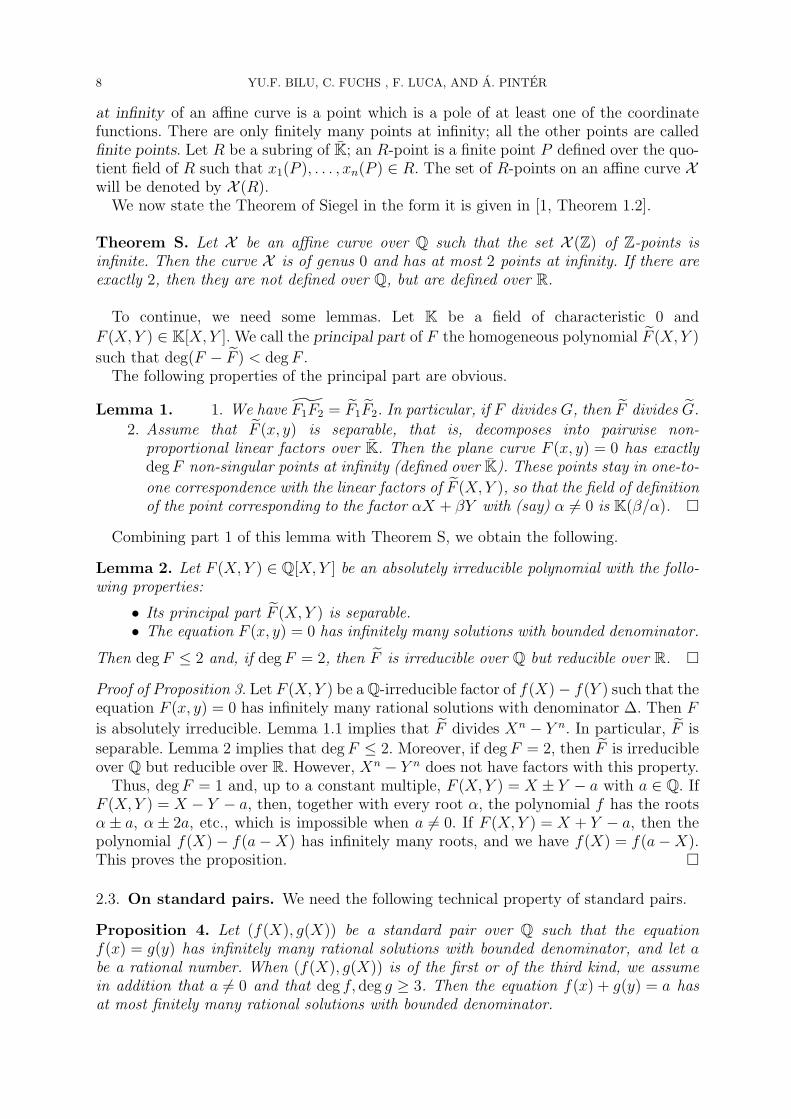
We now state the Theorem of Siegel in the form it is given in [1, Theorem 1.2].
Theorem S. Let X be an affine curve over Q such that the set X (Z) of Z-points isinfinite. Then the curve X is of genus 0 and has at most 2 points at infinity. If there areexactly 2, then they are not defined over Q, but are defined over R.
To continue, we need some lemmas. Let K be a field of characteristic 0 and
F (X, Y ) ∈ K[X, Y ]. We call the principal part of F the homogeneous polynomial F (X, Y )
such that deg(F − F ) < degF .The following properties of the principal part are obvious.
Lemma 1. 1. We have F1F2 = F1F2. In particular, if F divides G, then F divides G.
2. Assume that F (x, y) is separable, that is, decomposes into pairwise non-proportional linear factors over K. Then the plane curve F (x, y) = 0 has exactlydegF non-singular points at infinity (defined over K). These points stay in one-to-
one correspondence with the linear factors of F (X, Y ), so that the field of definitionof the point corresponding to the factor αX + βY with (say) α 6= 0 is K(β/α). �
Combining part 1 of this lemma with Theorem S, we obtain the following.
Lemma 2. Let F (X, Y ) ∈ Q[X, Y ] be an absolutely irreducible polynomial with the follo-wing properties:
• Its principal part F (X, Y ) is separable.• The equation F (x, y) = 0 has infinitely many solutions with bounded denominator.
Then degF ≤ 2 and, if degF = 2, then F is irreducible over Q but reducible over R. �
Proof of Proposition 3. Let F (X, Y ) be a Q-irreducible factor of f(X)− f(Y ) such that theequation F (x, y) = 0 has infinitely many rational solutions with denominator ∆. Then F
is absolutely irreducible. Lemma 1.1 implies that F divides Xn − Y n. In particular, F is
separable. Lemma 2 implies that degF ≤ 2. Moreover, if degF = 2, then F is irreducibleover Q but reducible over R. However, Xn − Y n does not have factors with this property.
Thus, degF = 1 and, up to a constant multiple, F (X, Y ) = X ± Y − a with a ∈ Q. IfF (X, Y ) = X − Y − a, then, together with every root α, the polynomial f has the rootsα± a, α± 2a, etc., which is impossible when a 6= 0. If F (X, Y ) = X + Y − a, then thepolynomial f(X)− f(a−X) has infinitely many roots, and we have f(X) = f(a−X).This proves the proposition. �
2.3. On standard pairs. We need the following technical property of standard pairs.
Proposition 4. Let (f(X), g(X)) be a standard pair over Q such that the equationf(x) = g(y) has infinitely many rational solutions with bounded denominator, and let abe a rational number. When (f(X), g(X)) is of the first or of the third kind, we assumein addition that a 6= 0 and that deg f, deg g ≥ 3. Then the equation f(x) + g(y) = a hasat most finitely many rational solutions with bounded denominator.
COMBINATORIAL DIOPHANTINE EQUATIONS WITH SEPARATED VARIABLES 9
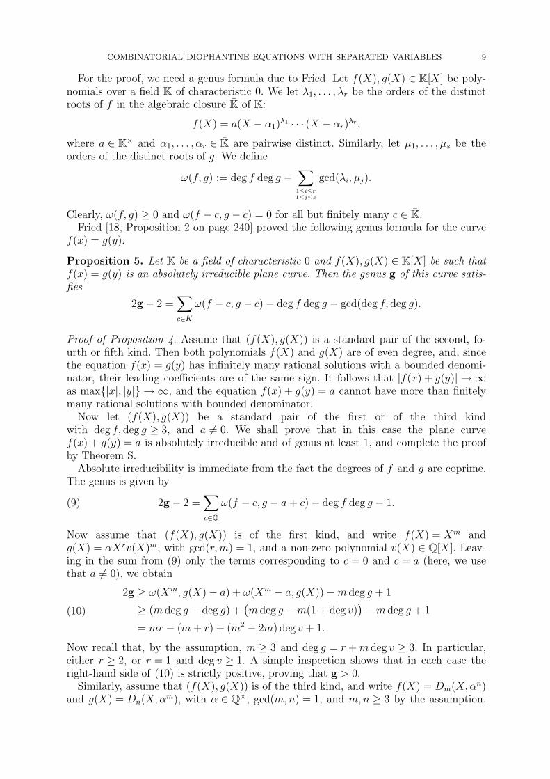
For the proof, we need a genus formula due to Fried. Let f(X), g(X) ∈ K[X] be poly-nomials over a field K of characteristic 0. We let λ1, . . . , λr be the orders of the distinctroots of f in the algebraic closure K of K:
f(X) = a(X − α1)λ1 · · · (X − αr)λr ,
where a ∈ K× and α1, . . . , αr ∈ K are pairwise distinct. Similarly, let µ1, . . . , µs be theorders of the distinct roots of g. We define
ω(f, g) := deg f deg g −∑1≤i≤r1≤j≤s
gcd(λi, µj).
Clearly, ω(f, g) ≥ 0 and ω(f − c, g − c) = 0 for all but finitely many c ∈ K.Fried [18, Proposition 2 on page 240] proved the following genus formula for the curve
f(x) = g(y).
Proposition 5. Let K be a field of characteristic 0 and f(X), g(X) ∈ K[X] be such thatf(x) = g(y) is an absolutely irreducible plane curve. Then the genus g of this curve satis-fies
2g − 2 =∑c∈K
ω(f − c, g − c)− deg f deg g − gcd(deg f, deg g).
Proof of Proposition 4. Assume that (f(X), g(X)) is a standard pair of the second, fo-urth or fifth kind. Then both polynomials f(X) and g(X) are of even degree, and, sincethe equation f(x) = g(y) has infinitely many rational solutions with a bounded denomi-nator, their leading coefficients are of the same sign. It follows that |f(x) + g(y)| → ∞as max{|x|, |y|} → ∞, and the equation f(x) + g(y) = a cannot have more than finitelymany rational solutions with bounded denominator.
Now let (f(X), g(X)) be a standard pair of the first or of the third kindwith deg f, deg g ≥ 3, and a 6= 0. We shall prove that in this case the plane curvef(x) + g(y) = a is absolutely irreducible and of genus at least 1, and complete the proofby Theorem S.
Absolute irreducibility is immediate from the fact the degrees of f and g are coprime.The genus is given by
(9) 2g − 2 =∑c∈Q
ω(f − c, g − a+ c)− deg f deg g − 1.
Now assume that (f(X), g(X)) is of the first kind, and write f(X) = Xm andg(X) = αXrv(X)m, with gcd(r,m) = 1, and a non-zero polynomial v(X) ∈ Q[X]. Leav-ing in the sum from (9) only the terms corresponding to c = 0 and c = a (here, we usethat a 6= 0), we obtain
2g ≥ ω(Xm, g(X)− a) + ω(Xm − a, g(X))−m deg g + 1
≥ (m deg g − deg g) +(m deg g −m(1 + deg v)
)−m deg g + 1
= mr − (m+ r) + (m2 − 2m) deg v + 1.
(10)
Now recall that, by the assumption, m ≥ 3 and deg g = r +m deg v ≥ 3. In particular,either r ≥ 2, or r = 1 and deg v ≥ 1. A simple inspection shows that in each case theright-hand side of (10) is strictly positive, proving that g > 0.
Similarly, assume that (f(X), g(X)) is of the third kind, and write f(X) = Dm(X,αn)and g(X) = Dn(X,αm), with α ∈ Q×, gcd(m,n) = 1, and m,n ≥ 3 by the assumption.
10 YU.F. BILU, C. FUCHS , F. LUCA, AND A. PINTER
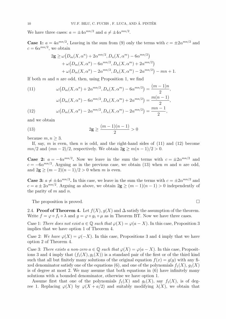
We have three cases: a = ±4αmn/2 and a 6= ±4αmn/2.
Case 1: a = 4αmn/2. Leaving in the sum from (9) only the terms with c = ±2αmn/2 andc = 6αmn/2, we obtain
2g ≥ω(Dm(X,αn) + 2αmn/2, Dn(X,αm)− 6αmn/2
)+ ω
(Dm(X,αn)− 6αmn/2, Dn(X,αm) + 2αmn/2
)+ ω
(Dm(X,αn)− 2αmn/2, Dn(X,αm)− 2αmn/2
)−mn+ 1.
If both m and n are odd, then, using Proposition 1, we find
ω(Dm(X,αn) + 2αmn/2, Dn(X,αm)− 6αmn/2
)=
(m− 1)n
2,(11)
ω(Dm(X,αn)− 6αmn/2, Dn(X,αm) + 2αmn/2
)=m(n− 1)
2,
ω(Dm(X,αn)− 2αmn/2, Dn(X,αm)− 2αmn/2
)=mn− 1
2,(12)
and we obtain
(13) 2g ≥ (m− 1)(n− 1)
2> 0
because m,n ≥ 3.If, say, m is even, then n is odd, and the right-hand sides of (11) and (12) become
mn/2 and (mn− 2)/2, respectively. We obtain 2g ≥ m(n− 1)/2 > 0.
Case 2: a = −4αmn/2. Now we leave in the sum the terms with c = ±2αmn/2 andc = −6αmn/2. Arguing as in the previous case, we obtain (13) when m and n are odd,and 2g ≥ (m− 2)(n− 1)/2 > 0 when m is even.
Case 3: a 6= ±4αmn/2. In this case, we leave in the sum the terms with c = ±2αmn/2 andc = a± 2αmn/2. Arguing as above, we obtain 2g ≥ (m− 1)(n− 1) > 0 independently ofthe parity of m and n.
The proposition is proved. �
2.4. Proof of Theorem 4. Let f(X), g(X) and ∆ satisfy the assumption of the theorem.Write f = ϕ ◦ f1 ◦ λ and g = ϕ ◦ g1 ◦ µ as in Theorem BT. Now we have three cases.
Case 1: There does not exist a ∈ Q such that ϕ(X) = ϕ(a−X). In this case, Proposition 3implies that we have option 1 of Theorem 4.
Case 2: We have ϕ(X) = ϕ(−X). In this case, Propositions 3 and 4 imply that we haveoption 2 of Theorem 4.
Case 3: There exists a non-zero a ∈ Q such that ϕ(X) = ϕ(a−X). In this case, Proposit-ions 3 and 4 imply that (f1(X), g1(X)) is a standard pair of the first or of the third kindsuch that all but finitely many solutions of the original equation f(x) = g(y) with any fi-xed denominator satisfy one of the equations (6), and one of the polynomials f1(X), g1(X)is of degree at most 2. We may assume that both equations in (6) have infinitely manysolutions with a bounded denominator, otherwise we have option 1.
Assume first that one of the polynomials f1(X) and g1(X), say f1(X), is of deg-ree 1. Replacing ϕ(X) by ϕ(X + a/2) and suitably modifying λ(X), we obtain that
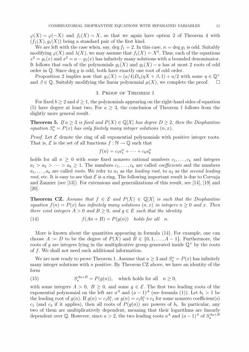
COMBINATORIAL DIOPHANTINE EQUATIONS WITH SEPARATED VARIABLES 11
ϕ(X) = ϕ(−X) and f1(X) = X, so that we again have option 2 of Theorem 4 with(f1(X), g1(X)) being a standard pair of the first kind.
We are left with the case when, say, deg f1 = 2. In this case, n = deg g1 is odd. Suitablymodifying ϕ(X) and λ(X), we may assume that f1(X) = X2. Thus, each of the equationsx2 = g1(x) and x2 = a− g1(x) has infinitely many solutions with a bounded denominator.It follows that each of the polynomials g1(X) and g1(X)− a has at most 2 roots of oddorder in Q. Since deg g is odd, both have exactly one root of odd order.
Proposition 2 implies now that g1(X) = (a/4)Dn(ηX + β, 1) + a/2 with some η ∈ Q×and β ∈ Q. Suitably modifying the linear polynomial µ(X), we complete the proof. �
3. Proof of Theorem 1
For fixed b ≥ 2 and d ≥ 1, the polynomials appearing on the right-hand sides of equation(5) have degree at least two. For a ≥ 3, the conclusion of Theorem 1 follows from theslightly more general result.
Theorem 5. If a ≥ 3 is fixed and P (X) ∈ Q[X] has degree D ≥ 2, then the Diophantineequation Sna = P (x) has only finitely many integer solutions (n, x).
Proof. Let E denote the ring of all exponential polynomials with positive integer roots.That is, E is the set of all functions f : N→ Q such that
f(n) = c1an1 + · · ·+ cka
nk
holds for all n ≥ 0 with some fixed nonzero rational numbers c1, . . . , ck and integersa1 > a2 > · · · > ak ≥ 1. The numbers c1, . . . , ck are called coefficients and the numbersa1, . . . , ak are called roots. We refer to a1 as the leading root, to a2 as the second leadingroot, etc. It is easy to see that E is a ring. The following important result is due to Corvajaand Zannier (see [13]). For extensions and generalizations of this result, see [14], [19] and[20].
Theorem CZ. Assume that f ∈ E and P (X) ∈ Q[X] is such that the Diophantineequation f(n) = P (x) has infinitely many solutions (n, x) in integers n ≥ 0 and x. Thenthere exist integers A > 0 and B ≥ 0, and g ∈ E such that the identity
(14) f(An+B) = P (g(n)) holds for all n.
More is known about the quantities appearing in formula (14). For example, one canchoose A := D to be the degree of P (X) and B ∈ {0, 1, . . . , A − 1}. Furthermore, theroots of g are integers lying in the multiplicative group generated inside Q× by the rootsof f . We shall not need such additional information.
We are now ready to prove Theorem 1. Assume that a ≥ 3 and Sna = P (x) has infinitelymany integer solutions with n positive. By Theorem CZ above, we have an identity of theform
(15) SAn+Ba = P (g(n)), which holds for all n ≥ 0,
with some integers A > 0, B ≥ 0, and some g ∈ E . The first two leading roots of theexponential polynomial on the left are aA and (a − 1)A (see formula (1)). Let b1 > 1 bethe leading root of g(n). If g(n) = c1b
n1 , or g(n) = c1b
n1 + c2 for some nonzero coefficient(s)
c1 (and c2 if it applies), then all roots of P (g(n)) are powers of b1. In particular, anytwo of them are multiplicatively dependent, meaning that their logarithms are linearlydependent over Q. However, since a > 2, the two leading roots aA and (a− 1)A of SAn+B
a
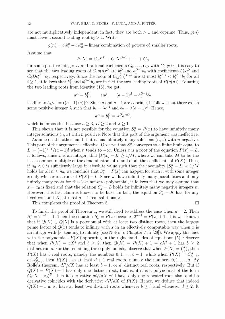
12 YU.F. BILU, C. FUCHS , F. LUCA, AND A. PINTER
are not multiplicatively independent; in fact, they are both > 1 and coprime. Thus, g(n)must have a second leading root b2 > 1. Write
g(n) = c1bn1 + c2b
n2 + linear combination of powers of smaller roots.
Assume that
P (X) = C0XD + C1X
D−1 + · · ·+ CD
for some positive integer D and rational coefficients C0, . . . , CD with C0 6= 0. It is easy tosee that the two leading roots of C0g(n)D are bD1 and bD−1
1 b2 with coefficients C0cD1 and
C0DcD−11 c2, respectively. Since the roots of Cig(n)D−i are at most bD−i1 < bD−1
1 b2 for alli ≥ 1, it follows that bD1 and bD−1
1 b2 are in fact the two leading roots of P (g(n)). Equatingthe two leading roots from identity (15), we get
aA = bD1 , and (a− 1)A = bD−11 b2,
leading to b2/b1 = ((a−1)/a))A. Since a and a−1 are coprime, it follows that there existssome positive integer λ such that b1 = λaA and b2 = λ(a− 1)A. Hence,
aA = bD1 = λDaAD,
which is impossible because a ≥ 3, D ≥ 2 and λ ≥ 1.This shows that it is not possible for the equation Sna = P (x) to have infinitely many
integer solutions (n, x) with n positive. Note that this part of the argument was ineffective.Assume on the other hand that it has infinitely many solutions (n, x) with n negative.
This part of the argument is effective. Observe that Sna converges to a finite limit equal toL := (−1)a−1/(a− 1)! when n tends to −∞. Unless x is a root of the equation P (x) = L,it follows, since x is an integer, that |P (x)− L| ≥ 1/M , where we can take M to be theleast common multiple of the denominators of L and of all the coefficients of P (X). Thus,if n0 < 0 is sufficiently large in absolute value such that the inequality |Sna − L| < 1/Mholds for all n ≤ n0, we conclude that Sna = P (x) can happen for such n with some integerx only when x is a root of P (X)−L. Since we have infinitely many possibilities and onlyfinitely many roots for this last nonzero polynomial, it follows that we may assume thatx = x0 is fixed and that the relation Sna = L holds for infinitely many negative integers n.However, this last claim is known to be false. In fact, the equation Sxa = K has, for anyfixed constant K, at most a− 1 real solutions x.
This completes the proof of Theorem 5. �
To finish the proof of Theorem 1, we still need to address the case when a = 2. ThenSna = 2n−1 − 1. Then the equation Sna = P (x) becomes 2n−1 = P (x) + 1. It is well-knownthat if Q(X) ∈ Q[X] is a polynomial with at least two distinct roots, then the largestprime factor of Q(x) tends to infinity with x in an effectively computable way when x isan integer with |x| tending to infinity (see Notes to Chapter 7 in [29]). We apply this factwith the polynomials P (X) appearing in the right-hand sides of equations (5). Observethat when P (X) = cXb and b ≥ 2, then Q(X) = P (X) + 1 = cXb + 1 has b ≥ 2distinct roots. For the remaining three polynomials, observe that when P (X) =
(Xb
), then
P (X) has b real roots, namely the numbers 0, 1, . . . , b − 1, while when P (X) = SXX−d,or sXX−d, then P (X) has at least d + 1 real roots, namely the numbers 0, 1, . . . , d. ByRolle’s theorem, dP/dX has at least b − 1, or d, distinct real roots, respectively. But ifQ(X) = P (X) + 1 has only one distinct root, that is, if it is a polynomial of the formC0(X − z0)D, then its derivative dQ/dX will have only one repeated root also, and itsderivative coincides with the derivative dP/dX of P (X). Hence, we deduce that indeedQ(X) + 1 must have at least two distinct roots whenever b ≥ 3 and whenever d ≥ 2. It
COMBINATORIAL DIOPHANTINE EQUATIONS WITH SEPARATED VARIABLES 13
remains to study the cases b = 2 and d = 1, for which P (X) =(X2
)= SXX−1 = sXX−1 and
for which P (X) + 1 =(X2
)+ 1 = (X2 − X + 2)/2 has two distinct roots anyway. Note
that this part of the proof is effective.This completes the proof of Theorem 1.
4. Proof of Theorem 2
All equations appearing in Theorem 2 are of the form p(x) = q(y), where p(X), q(X)are certain polynomials in Q[X], and thus we shall apply Theorem 4.
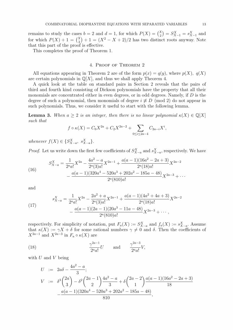
A quick look at the table on standard pairs in Section 2 reveals that the pairs ofthird and fourth kind consisting of Dickson polynomials have the property that all theirmonomials are concentrated either in even degrees, or in odd degrees. Namely, if D is thedegree of such a polynomial, then monomials of degree i 6≡ D (mod 2) do not appear insuch polynomials. Thus, we consider it useful to start with the following lemma.
Lemma 3. When a ≥ 2 is an integer, then there is no linear polynomial κ(X) ∈ Q[X]such that
f ◦ κ(X) = C0X2a + C2X
2a−2 +∑
0≤i≤2a−4
C2a−iXi,
whenever f(X) ∈ {SXX−a, sXX−a}.
Proof. Let us write down the first few coefficients of SXX−a and sXX−a, respectively. We have
SXX−a =1
2aa!X2a − 4a2 − a
2a(3)a!X2a−1 +
a(a− 1)(16a2 − 2a+ 3)
2a(18)a!X2a−2
− a(a− 1)(320a4 − 520a3 + 202a2 − 185a− 48)
2a(810)a!X2a−3 + · · ·
(16)
and
sXX−a =1
2aa!X2a − 2a2 + a
2a(3)a!X2a−1 +
a(a− 1)(4a2 + 4a+ 3)
2a(18)a!X2a−2
− a(a− 1)(2a− 1)(20a3 − 11a− 48)
2a(810)a!X2a−3 + · · · ,
(17)
respectively. For simplicity of notation, put Fa(X) := SXX−a and fa(X) := sXX−a. Assumethat κ(X) := γX + δ for some rational numbers γ 6= 0 and δ. Then the coefficients ofX2a−1 and X2a−3 in Fa ◦ κ(X) are
(18)γ2a−1
2aa!U and
γ2a−3
2aa!V,
with U and V being
U := 2aδ − 4a2 − a3
;
V := δ3
(2a
3
)− δ2
(2a− 1
2
)4a2 − a
3+ δ
(2a− 2
1
)a(a− 1)(16a2 − 2a+ 3)
18
−a(a− 1)(320a4 − 520a3 + 202a2 − 185a− 48)
810,
14 YU.F. BILU, C. FUCHS , F. LUCA, AND A. PINTER
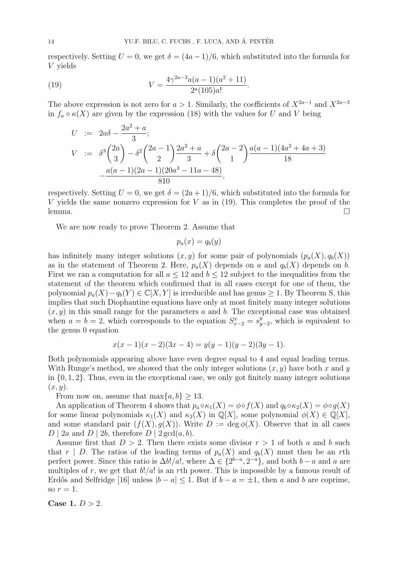
respectively. Setting U = 0, we get δ = (4a− 1)/6, which substituted into the formula forV yields
(19) V =4γ2a−3a(a− 1)(a2 + 11)
2a(105)a!.
The above expression is not zero for a > 1. Similarly, the coefficients of X2a−1 and X2a−3
in fa ◦ κ(X) are given by the expression (18) with the values for U and V being
U := 2aδ − 2a2 + a
3;
V := δ3
(2a
3
)− δ2
(2a− 1
2
)2a2 + a
3+ δ
(2a− 2
1
)a(a− 1)(4a2 + 4a+ 3)
18
−a(a− 1)(2a− 1)(20a3 − 11a− 48)
810,
respectively. Setting U = 0, we get δ = (2a+ 1)/6, which substituted into the formula forV yields the same nonzero expression for V as in (19). This completes the proof of thelemma. �
We are now ready to prove Theorem 2. Assume that
pa(x) = qb(y)
has infinitely many integer solutions (x, y) for some pair of polynomials (pa(X), qb(X))as in the statement of Theorem 2. Here, pa(X) depends on a and qb(X) depends on b.First we ran a computation for all a ≤ 12 and b ≤ 12 subject to the inequalities from thestatement of the theorem which confirmed that in all cases except for one of them, thepolynomial pa(X)−qb(Y ) ∈ C[X, Y ] is irreducible and has genus ≥ 1. By Theorem S, thisimplies that such Diophantine equations have only at most finitely many integer solutions(x, y) in this small range for the parameters a and b. The exceptional case was obtainedwhen a = b = 2, which corresponds to the equation Sxx−2 = syy−2, which is equivalent tothe genus 0 equation
x(x− 1)(x− 2)(3x− 4) = y(y − 1)(y − 2)(3y − 1).
Both polynomials appearing above have even degree equal to 4 and equal leading terms.With Runge’s method, we showed that the only integer solutions (x, y) have both x and yin {0, 1, 2}. Thus, even in the exceptional case, we only got finitely many integer solutions(x, y).
From now on, assume that max{a, b} ≥ 13.An application of Theorem 4 shows that pa◦κ1(X) = φ◦f(X) and qb◦κ2(X) = φ◦g(X)
for some linear polynomials κ1(X) and κ2(X) in Q[X], some polynomial φ(X) ∈ Q[X],and some standard pair (f(X), g(X)). Write D := deg φ(X). Observe that in all casesD | 2a and D | 2b, therefore D | 2 gcd(a, b).
Assume first that D > 2. Then there exists some divisor r > 1 of both a and b suchthat r | D. The ratios of the leading terms of pa(X) and qb(X) must then be an rthperfect power. Since this ratio is ∆b!/a!, where ∆ ∈ {2b−a, 2−a}, and both b− a and a aremultiples of r, we get that b!/a! is an rth power. This is impossible by a famous result ofErdos and Selfridge [16] unless |b− a| ≤ 1. But if b− a = ±1, then a and b are coprime,so r = 1.
Case 1. D > 2.
COMBINATORIAL DIOPHANTINE EQUATIONS WITH SEPARATED VARIABLES 15
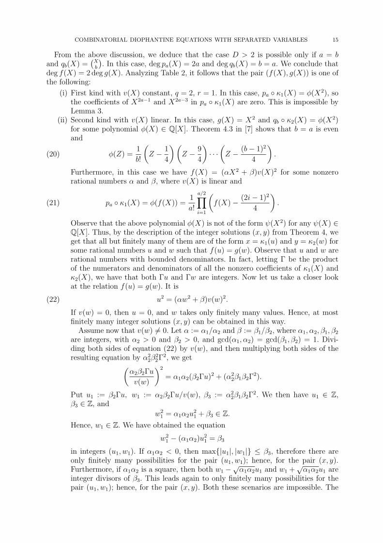
From the above discussion, we deduce that the case D > 2 is possible only if a = band qb(X) =
(Xb
). In this case, deg pa(X) = 2a and deg qb(X) = b = a. We conclude that
deg f(X) = 2 deg g(X). Analyzing Table 2, it follows that the pair (f(X), g(X)) is one ofthe following:
(i) First kind with v(X) constant, q = 2, r = 1. In this case, pa ◦ κ1(X) = φ(X2), sothe coefficients of X2a−1 and X2a−3 in pa ◦ κ1(X) are zero. This is impossible byLemma 3.
(ii) Second kind with v(X) linear. In this case, g(X) = X2 and qb ◦ κ2(X) = φ(X2)for some polynomial φ(X) ∈ Q[X]. Theorem 4.3 in [7] shows that b = a is evenand
(20) φ(Z) =1
b!
(Z − 1
4
)(Z − 9
4
)· · ·(Z − (b− 1)2
4
).
Furthermore, in this case we have f(X) = (αX2 + β)v(X)2 for some nonzerorational numbers α and β, where v(X) is linear and
(21) pa ◦ κ1(X) = φ(f(X)) =1
a!
a/2∏i=1
(f(X)− (2i− 1)2
4
).
Observe that the above polynomial φ(X) is not of the form ψ(X2) for any ψ(X) ∈Q[X]. Thus, by the description of the integer solutions (x, y) from Theorem 4, weget that all but finitely many of them are of the form x = κ1(u) and y = κ2(w) forsome rational numbers u and w such that f(u) = g(w). Observe that u and w arerational numbers with bounded denominators. In fact, letting Γ be the productof the numerators and denominators of all the nonzero coefficients of κ1(X) andκ2(X), we have that both Γu and Γw are integers. Now let us take a closer lookat the relation f(u) = g(w). It is
(22) u2 = (αw2 + β)v(w)2.
If v(w) = 0, then u = 0, and w takes only finitely many values. Hence, at mostfinitely many integer solutions (x, y) can be obtained in this way.
Assume now that v(w) 6= 0. Let α := α1/α2 and β := β1/β2, where α1, α2, β1, β2
are integers, with α2 > 0 and β2 > 0, and gcd(α1, α2) = gcd(β1, β2) = 1. Divi-ding both sides of equation (22) by v(w), and then multiplying both sides of theresulting equation by α2
2β22Γ2, we get(
α2β2Γu
v(w)
)2
= α1α2(β2Γu)2 + (α22β1β2Γ2).
Put u1 := β2Γu, w1 := α2β2Γu/v(w), β3 := α22β1β2Γ2. We then have u1 ∈ Z,
β3 ∈ Z, and
w21 = α1α2u
21 + β3 ∈ Z.
Hence, w1 ∈ Z. We have obtained the equation
w21 − (α1α2)u2
1 = β3
in integers (u1, w1). If α1α2 < 0, then max{|u1|, |w1|} ≤ β3, therefore there areonly finitely many possibilities for the pair (u1, w1); hence, for the pair (x, y).Furthermore, if α1α2 is a square, then both w1 −
√α1α2u1 and w1 +
√α1α2u1 are
integer divisors of β3. This leads again to only finitely many possibilities for thepair (u1, w1); hence, for the pair (x, y). Both these scenarios are impossible. The
16 YU.F. BILU, C. FUCHS , F. LUCA, AND A. PINTER
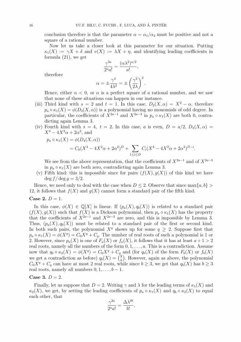
conclusion therefore is that the parameter α = α1/α2 must be positive and not asquare of a rational number.
Now let us take a closer look at this parameter for our situation. Puttingκ1(X) := γX + δ and v(X) := λX + η, and identifying leading coefficients informula (21), we get
γ2a
2aa!=
(αλ2)a/2
a!,
therefore
α = ± γ4
4λ2= ±
(γ2
2λ
)2
.
Hence, either α < 0, or α is a perfect square of a rational number, and we sawthat none of these situations can happen in our instance.
(iii) Third kind with s = 2 and t = 1. In this case, D2(X,α) = X2 − α, thereforepa ◦ κ1(X) = φ(D2(X,α)) is a polynomial having no monomials of odd degree. Inparticular, the coefficients of X2a−1 and X2a−3 in pa ◦ κ1(X) are both 0, contra-dicting again Lemma 3.
(iv) Fourth kind with s = 4, t = 2. In this case, a is even, D = a/2, D4(X,α) =X4 − 4X2α + 2α2, and
pa ◦ κ1(X) = φ(D4(X,α))
= C0(X4 − 4X2α + 2α2)D +∑
1≤i≤D
Ci(X4 − 4X2α + 2α2)D−i.
We see from the above representation, that the coefficients of X2a−1 and of X2a−3
in pa ◦ κ1(X) are both zero, contradicting again Lemma 3.(v) Fifth kind: this is impossible since for pairs (f(X), g(X)) of this kind we have
deg f/ deg g = 3/2.
Hence, we need only to deal with the case when D ≤ 2. Observe that since max{a, b} >12, it follows that f(X) and g(X) cannot form a standard pair of the fifth kind.
Case 2. D = 1.
In this case, φ(X) ∈ Q[X] is linear. If (pa(X), qb(X)) is related to a standard pair(f(X), g(X)) such that f(X) is a Dickson polynomial, then pa ◦ κ1(X) has the propertythat the coefficients of X2a−1 and X2a−3 are zero, and this is impossible by Lemma 3.Thus, (pa(X), qb(X)) must be related to a standard pair of the first or second kind.In both such pairs, the polynomial Xq shows up for some q ≥ 2. Suppose first thatpa ◦ κ1(X) = φ(Xq) = C0X
q + Cq. The number of real roots of such a polynomial is 1 or2. However, since pa(X) is one of Fa(X) or fa(X), it follows that it has at least a+ 1 > 2real roots, namely all the numbers of the form 0, 1, . . . , a. This is a contradiction. Assumenow that qb ◦ κ2(X) = φ(Xq) = C0X
q + Cq and (for qb(X) of the form Fb(X) or fb(X)
we get a contradiction as before) qb(X) =(Xb
). However, again as above, the polynomial
C0Xq + Cq can have at most 2 real roots, while since b ≥ 3, we get that qb(X) has b ≥ 3
real roots, namely all numbers 0, 1, . . . , b− 1.
Case 3. D = 2.
Finally, let us suppose that D = 2. Writing γ and λ for the leading terms of κ1(X) andκ2(X), we get, by setting the leading coefficients of pa ◦ κ1(X) and qb ◦ κ2(X) to equaleach other, that
γ2a
2aa!=
∆λδb
b!,
COMBINATORIAL DIOPHANTINE EQUATIONS WITH SEPARATED VARIABLES 17
where (∆, δ) := (1, 1) if qb(X) =(Xb
), and (∆, δ) := (2−b, 2) if qb(X) is one of Fb(X) and
fb(X). In the first case, since D divides the degree of qb(X), it follows that b is even, whilein the second case δb is even. Thus, in all instances we get that a!/b! is a square or twicetimes a square. Hence, |b− a| ≤ 2, by a result from [16] (see also [4]).
Assume now that (pa(X), qb(X)) is related to a standard pair involving Dickson poly-nomials. Then
pa ◦ κ1(X) = C0Da(X,α)2 + C1Da(X,α) + C2.
Observe that Da(X,α)2 has no monomials of odd order in it. Thus, if a > 3, then 2a−3 >a = deg(Da(X,α)), so that X2a−1 and X2a−3 do not appear in pa ◦ κ1(X), which is incontradiction with Lemma 3. But if a ≤ 3, then b ≤ 5, and this is impossible sincemax{a, b} ≥ 13.
Assume now that (pa(X), qb(X)) is related to one of the standard pairs of first orsecond kind. Say pa(X) = C0x
2q +C1Xq +C2. The derivative of such a polynomial, which
is qXq−1(2C0Xq +C1), has at most three distinct real roots. But pa(X) has a+ 1 distinct
real roots, so the derivative of pa ◦ κ1(X) has at least a distinct real roots by Rolle’stheorem. We get a contradiction for a ≥ 4. But if a ≤ 3, then b ≤ 5, which is not allowed.A similar argument applies when qb(X) = C0X
2q +C1Xq +C2 and qb(X) is one of Fb(X)
or fb(X) (with b ≥ 4), or qb(X) =(Xb
)(with b ≥ 5). But if b ≤ 4, then a ≤ 6, which again
is not allowed.This completes the proof of Theorem 2.
5. Proof of Theorem 3
Our equation can be rewritten as 8Sxx−a+1 = (2y−1)2. In order to prove that it has onlyfinitely many integer solutions (x, y), it suffices, via Baker’s theorem on integral solutionsof hyperelliptic equations (cf. [2]), to prove that the polynomial 8Fa(X) + 1 = 8SXX−a + 1has at least three roots of odd multiplicities. We shall assume that this is not so and arriveat a contradiction. We start with a lemma concerning the size of the roots of 8SXX−a + 1.
Lemma 4. If a ≥ 2 and z ∈ C is a zero of 8SXX−a + 1, then we have |z| < 10a2.
Proof. We know that the sequence {Sa+kk }k=1,...,a is log-concave (see page 81 in [9]). In
particular, the sequence
Sa+kk
Sa+k+1k+1
for k = 1, 2, . . . , a− 1
is increasing with the maximal value being
S2a−1a−1
S2aa
=a− 1
3.
Suppose now that |z| ≥ 10a2 is a root of this polynomial. In particular, |z| > 2a, so that(z)2a = z(z − 1) · · · (z − (2a− 1)) 6= 0. Rewrite the fact that Szz−a = −1/8 as
(23)a−1∑k=1
(2a)!
(a+ k)!
(z)a+k
(z)2a
Sa+kk
S2aa
= −1
8− (2a)!
S2aa (z)2a
.
We take absolute values in equation (23) above and apply the absolute value inequality.Since S2a
a is an integer, |(z)2a| > (10a2− 2a)2a > (8a)2a and (2a)! < (2a)2a, it follows that∣∣∣∣ (2a)!
S2aa (z)2a
∣∣∣∣ ≤ (2a)2a
(8a)2a=
1
42a,
18 YU.F. BILU, C. FUCHS , F. LUCA, AND A. PINTER
therefore the absolute value of the right-hand side of relation (23) above is
≥ 1
8− 1
42a>
1
9
for a ≥ 2. In the left-hand side of relation (23), we apply the absolute value inequalitygetting
(24)a−1∑k=1
(a+ k + 1) · · · (2a)
(|z| − (a+ k)) · · · (|z| − (2a− 1))
Sa+kk
S2aa
>1
9.
Clearly,
(a+ k + 1) · · · (2a) < (2a)a−k;
1
(|z| − (a+ k)) · · · (|z| − (2a− 1))<
(1
10a2 − 2a
)a−k≤ 1
5
(1
2a(a− 1)
)a−k;
Sa+kk
S2aa
=Sa+kk
Sa+k+1k+1
· · ·S2a−1a−1
S2aa
≤(a− 1
3
)a−kfor all k = 1, 2, . . . , a−1. Multiplying the above inequalities, we get that the general termin the sum appearing in the left-hand side of (24) is
(a+ k + 1) · · · (2a)
(|z| − (a+ k)) · · · (|z| − (2a− 1))
Sa+kk
S2aa
<1
5
(1
3
)a−k.
Hence, inequality (24) leads to
1
9<
1
5
a−1∑k=1
(1
3
)a−k<
1
5
∑m≥1
(1
3
)m=
1
10,
which is a contradiction. �
A quick computation of some of the values of its coefficients (see equations (16), forexample) gives us that
8SXX−a + 1 =X2a
2a−3a!− (4a2 − a)X2a−1
2a−3 · 3 · a!+a(a− 1)(16a2 − 2a+ 3)X2a−2
2a−3 · 18 · a!
− a(a− 1)(320a4 − 520a3 + 202a2 − 185a− 48)x2a−3
2a−3 · 810 · a!+ · · ·+ 1
for a ≥ 2. Since it has even degree 2a, it follows that it has an even number of roots ofodd multiplicity. If this even number is 0, we then get that the relation
8SXX−a + 1 = a0f(X)2
holds with some monic polynomial f(X) with rational coefficients, where a0 := 1/(2a−3a!)is the leading coefficient of 8SXX−a + 1. Putting x := 0, we get
f(0)2 =1
a0
= 2a−3a!,
but this is impossible for any a ≥ 3, since by Bertrand’s postulate, the interval (a/2, a]always contains a prime p ≥ 3 for a ≥ 3. Such a prime p has the property that p‖2a−3a!,so 2a−3a! cannot be the square of a rational number when a ≥ 3.
COMBINATORIAL DIOPHANTINE EQUATIONS WITH SEPARATED VARIABLES 19
It remains to deal with the case when 8SXX−a + 1 has two roots of odd multiplicity. Inthis case, we write
(25) 8SXX−a + 1 = a0f(X)g(X)2,
where f(X) := (X − x1)(X − x2). Clearly, f(X) ∈ Q[X], so either x1 and x2 are bothrational, or the quadratic polynomial f(X) is irreducible over Q and then x1 and x2 arequadratic and conjugate. Now let us make some remarks about the polynomial
a−10 (8SXX−a + 1).
It is a monic polynomial. Using formula (2), we get that this polynomial is
(26) (X)2a +a−1∑k=1
(X)a+k2aa!
(a+ k)!Sa+kk + 2a−3a!.
We write the above polynomial (26) as
X2a − (4a2 − n)
3X2a−1 +
a(a− 1)(16a2 − 2a+ 3)X2a−2
18
− a(a− 1)(320a4 − 520a3 + 202a2 − 185a− 48)X2a−3
810+ · · ·+ 2a−3a!
=:2a∑k=0
ckX2a−k.
Let us get a handle on the denominators of the coefficients ck for k = 0, . . . , 2a. Write
2aa!
(a+ k)!Sa+kk :=
aa,kba,k
,
where aa,k and ba,k are coprime integers. We need to understand the numbers ba,k andtheir least common multiple, which we denote by D, as k varies in {1, . . . , a− 1}.
Now a formula from page 222 in [12], tells us that Sa+kk is a multiple of 1 · 3 · · · (2k− 1).
Thus, aa,k/ba,k is an integer multiple of the rational number
2aa! · 1 · 3 · · · (2k − 1)
(a+ k)!=
2aa!(2k)!
2kk!(a+ k)!=
2a−ka!(2k)!
k!(a+ k)!.
Let p be an arbitrary prime with 2 ≤ p < 2a. Let us find an upper bound for its exponentin ba,k. Writing νp(r) for the exponent of p in the factorization of r and using the fact thatthe formula
νp(m!) =∑s≥1
⌊m
ps
⌋holds for all positive integers m, it follows that the exponent of p in ba,k satisfies
(27) νp(ba,k) ≤∑s≥1
(⌊a+ k
ps
⌋−⌊a
ps
⌋)+
(⌊k
ps
⌋−⌊
2k
ps
⌋).
Clearly, ⌊a+ k
ps
⌋−⌊a
ps
⌋∈{⌊
k
ps
⌋,
⌊k
ps
⌋+ 1
},
and ⌊k
ps
⌋−⌊
2k
ps
⌋∈{−⌊k
ps
⌋, −
⌊k
ps
⌋− 1
},
20 YU.F. BILU, C. FUCHS , F. LUCA, AND A. PINTER
together implying that for a fixed s ≥ 1, we have(⌊a+ k
ps
⌋−⌊a
ps
⌋)+
(⌊k
ps
⌋−⌊
2k
ps
⌋)∈ {0,±1}.
Suppose now that a ≥ 1000. Suppose also that p ≥ a/22. Then p2 ≥ a2/222 > 2a. Thus,in formula (27) we have that
νp(ba,k) ≤ 1 for p ≥ a/22 assuming that a ≥ 1000.
For the remaining primes p < a/22, we have that
νp(ba,k) ≤∑s≥1ps≤2a
1 ≤ log(2a)
log p.
Hence, we have that
B :=∏
pap‖lcm[ba,k:1≤k≤a−1]p<a/22
pap ≤∏
p<a/22
plog(2a)/ log p ≤ (2a)π(a/22).
We conclude that
D := lcm[ba,k : 1 ≤ k ≤ a− 1] = BC,
where
(28) B =∏pap
p<a/22
pap < exp(π( a
22
)log(2a)
), and C :=
∏a/22≤p≤2abp∈{0,1}
pbp .
Now let z ∈ {x1, x2} be some root of f(x). We first deal with the case when z is rational.It is clear that the denominator of z divides D but we can do better. Namely, we showthat the denominator of z divides B. Indeed, to see why, assume that p ≥ a/22 dividesthe denominator of z. Since C is squarefree, it follows that pz is a rational number havingboth numerator and denominator coprime to p. Multiplying relation
z2a − (4a2 − a)z2a−1
3+ · · ·+ 2a−3a! = 0
with p2a and regrouping, we get
(29) (pz)2a =p(4a2 − a)
3(pz)2a−1 −
2a∑k=2
pkck(pz)2a−k.
Since p > 3 (because a/22 > 3 for a ≥ 1000), and the denominator of ck is not amultiple of p2 for any k = 2, . . . , 2a, it follows easily that the right-hand side of theabove formula is a rational number whose numerator in reduced form is a multiple ofp, while the left-hand side is a rational number which in reduced form has numeratorcoprime to p. This contradiction shows that the denominator of z is a divisor of B. Wenow write x1 := u1/v1, x2 := u2/v2 with u1, u2, v1 > 0, v2 > 0 integers such thatgcd(u1, v1) = gcd(u2, v2) = 1, and evaluate relation (25) in x := 0 getting
2a−3n! = x1x2g(0)2,
In particular, it follows that u1u2 is a multiple of all primes p ∈ (a/2, a]. Hence,
(30) |u1u2| ≥∏
a/2<p≤a
p >(a
2
)π(a)−π(a/2)
.
COMBINATORIAL DIOPHANTINE EQUATIONS WITH SEPARATED VARIABLES 21
Thus,
(31) |u1u2| ≥(a
2
)π(a)−π(a/2)
.
Assuming say that |u1| ≥ |u2|, we conclude that
|u1| ≥ (|u1u2|)1/2 ≥ exp
(1
2
(π(a)− π
(a2
))log(a
2
)).
Hence, using the fact that v1 | B and estimate (28), we get that
|x1| = |u1|v−11 ≥ |u1|B−1
≥ exp
(1
2
(π(a)− π
(a2
))log(a
2
)− π
( a22
)log(2a)
).
However, Lemma 4 implies that |x1| ≤ 10a2. We thus get the inequality
(32) log(10a2) ≥ 1
2
(π(a)− π
(a2
))log(a
2
)− π
( a22
)log(2a).
Using the inequalitiesx
log x− 0.5< π(x) <
x
log x− 1.5for all x ≥ 67,
(see Theorem 2 in [27]) with x = a, a/2, and a/22 respectively, we get that
(33) log(10a2) ≥ 1
2
(a
log a− 0.5− a
2(log(a/2)− 1.5)
)log(a
2
)− a log(2a)
22(log(a/22)− 1.5)
for a ≥ 1474. The condition a ≥ 1474 arises from the condition a/22 ≥ 67, which isnecessary for Theorem 2 in [27] to apply. On the other hand, the inequality (33) aboveyields a < 1200. This shows that in fact the inequality a < 1474 must hold. Then we alsochecked that the inequality (32) holds for no a ∈ [1000, 1474]. Thus, we must in fact havea < 1000, assuming that one of (hence, both) x1 or x2 is rational.
From now on, we treat the slightly more complicated case of the quadratic roots x1 andx2. As in the previous case, we assume that a ≥ 1000 for this case also.
Let us write
x1,2 =u± v
√d
c,
where u, v, w > 0 and d 6= 1 are integers, with d squarefree. We may also assume thatthere is no common prime factor number dividing all three of u, v and c. Since Dx1,2 arealgebraic integers, it follows easily that c/ gcd(c,D) = 1, 2. The plan is to show that cand C are coprime. This will show that c ≤ 2B. Well, let’s do it. Assume that there issome prime p ≥ a/22 dividing c. We distinguish three possibilities:
(i) p - u2 − dv2;(ii) p | u2 − dv2, and p | u;
(iii) p | u2 − dv2, but p - u.
The first instance is similar to the case in which one of (hence, both) x1 or x2 are rationalwhose denominator is a multiple of p. Indeed, assuming that we are in Case (i) above,relation (29) with z = x1 has the property that the number appearing in its left-hand sideis a quadratic algebraic number whose norm is a rational number having both numeratorand denominator coprime to p. The right-hand side of the same relation however, is theproduct between p and a linear combination (with rational coefficients, the denominatorsof which are not multiples of p) of quadratic algebraic numbers the denominators of which
22 YU.F. BILU, C. FUCHS , F. LUCA, AND A. PINTER
are also coprime to p. Hence, upon taking norms in (29) relative to the quadratic fieldK := Q[x1], the left-hand side evaluates to a rational number having both numerator anddenominator coprime to p, while the right-hand side evaluates to a rational number whichin reduced form has its numerator a multiple of p. This is a contradiction.
A somewhat similar argument works for Case (ii). Here, one notices that with z := x1
we have
(pz)k =
(u+ v
√d
c/p
)k
= pk/2
(u/√p+ v
√d/p
c/p
)k
=: pk/2λk,
where λ := (u/√p+ v
√d/p)/(c/p) is a quadratic or bi-quadratic (depending on whether
d = p, or not) algebraic number, which is the ratio of two algebraic integers u/√p+v
√d/p
and c/p, having norms powers of (u2−dv2)/p and (c/p)2, which are both integers coprimeto p. Thus, relation (29) becomes
pnλ2a = pa(
(4a2 − a)
3p1/2λ2a−1 − a(a− 1)(16a2 − 2a+ 3)2a−2p
18λ2a−2
−2a∑k=3
pk/2ckλ2a−k
)=: paγ.
(34)
Observe that if k ≥ 3, then pk/2ckλ2a−k is the product between p1/2 and some algebraic
number the norm of which has denominator coprime to p. The same is true for k = 2since p ≥ a/22 > 3 (because a ≥ 1000). Thus, simplifying both sides of relation (34)by pa, putting β := γ/p1/2, and then taking norms in L := Q[p1/2, λ] of both sides ofthe resulting identity, we end up with an equality between NL(λ2a), which is a rationalnumber having numerator and denominator coprime to p, and NL(p1/2β) = p`NL(β), with` = 1 or 2, according to whether the degree of L over Q is 2 or 4, where NL(β) is a rationalnumber whose denominator is coprime to p. This is a contradiction.
Finally, let us look at the possible primes occurring in Case (iii). In this case, x1 +x2 =u/c = d1/p, where d1 is some rational number having both numerator and denominatorcoprime to p. Observe also that x1x2 = (u2 − dv2)/c2. We distinguish two cases.
Case (iii).1 p‖u2 − dv2.
In this case,
f(x) = x2 +d1x
p+d2
p,
where d2 is a rational number having numerator and denominator coprime to p. We write
(35) g(x)2 = x2a−2 + e1x2a−3 + e2x
2a−4 + · · ·+ e2a−2,
and prove by induction on m ≥ 1 that em = fm/pm, where fm is a rational number
having numerator and denominator coprime to p. Indeed, multiplying f(x) with g(x)2
and identifying coefficients, we get
f(x)g(x)2 = x2a − (4a2 − a)
3x2a−1 +
a(a− 1)(16a2 − 2a+ 3)
18x2a−2 + · · ·
= x2a +
(d1
p+ e1
)x2a−1 +
(d2
p+d1e1
p+ e2
)x2a−2 + · · · .
Since the denominator of (4a2 − a)/3 is not a multiple of p, we get that e1 = f1/p withf1 a rational number whose numerator and denominator is coprime to p. Thus, indeed e1
COMBINATORIAL DIOPHANTINE EQUATIONS WITH SEPARATED VARIABLES 23
has the desired shape. Now
c2 =d2
p+d1e1
p+ e2 =
d2
p+d1f1
p2+ e2,
and the denominator of c2 is not a multiple of p, showing that e2 = f2/p2, where the
numerator and denominator of f2 are coprime to p. Assuming that ei has the desiredshape fi/p for i = 1, . . . ,m and some 1 < m < 2a − 2, and computing the coefficient ofx2a−(m−1), we get
cm+1 =d2em−1
p+d1emp
+ em+1 =d2fm−1
pm+d1fmpm+1
+ em+1.
Since the denominator of cm+1 is not divisible by p2, we get that indeed em+1 = fm+1/pm+1
for some rational number fm+1 having numerator and denominator both coprime to p.Thus, the last coefficient of f(x)g(x)2 is d2e2a−2/p = d2f2a−2/p
2a−1, which is impossiblesince this coefficient must be the integer 2a−3a!. Hence, this case is impossible.
Case (iii).2 p2 | u2 − dv2.
Part of this case is similar to the previous one. Here, we have
f(x) = x2 +d1x
p+ d2,
where d2 is a rational number whose denominator is coprime to p. In the notation (35),one gets that
f(x)g(x)2 = x2a +
(d1
p+ e1
)x2a−1 +
(d2 +
d1e1
p+ e2
)x2a−2 + · · ·
From the above, we see right away that e1 = f1/p, where f1 is a rational number whosenumerator and denominator are coprime to p, and then that
c2 = d2 +d1e1
p+ e2 = d2 +
d1f1
p2+ e2.
Since the denominator of c2 is not a multiple of p, we get that e2 = f2/p2, where f2 is a
rational number whose numerator and denominator are coprime to p. By induction overm ≥ 1, we get as in the previous case that em = fm/p
m, where fm is a rational numberwhose numerator and denominator are coprime to p. For the induction step, we use theformula
cm+1 = d2em−1 +d1emp
+ em+1 =d2fm−1
pm−1+d1fmpm+1
+ em+1.
By looking at the last coefficients, we have d2e2a−2 = d2f2a−2/p2a−2. Since this last co-
efficient is in fact an integer, it follows that νp(d2) ≥ 2a − 2, which in turn implies thatνp(u
2 − dv2) ≥ 2a.Hence, so far, we conclude that if c has prime factors p in [a/22, 2a], then νp(u
2−dv2) ≥2a. Now write
c = c1C1,
where C1 = gcd(c, C) and c1 | 2B. It then follows that
|u2 − dv2| ≥ C2a1 ,
so that
|x1x2| =∣∣∣∣u2 − dv2
c2
∣∣∣∣ =
∣∣∣∣u2 − dv2
c21C
21
∣∣∣∣ ≥ C2a−21 (2B)−2.
24 YU.F. BILU, C. FUCHS , F. LUCA, AND A. PINTER
Using Lemma 4 and inequality (28) we arrive at
400a4(2a)2π(a/22) > C2a−21 .
Assuming that C1 > 1, and using the trivial fact that π(x) < x, we are led to the inequality
400a4(2a)a/11 >( a
22
)2a−2
,
which is false for any a ≥ 40. So, this case cannot occur either.Hence, we have just shown that c divides 2B. Thus, 4B2|x1x2| is an integer which, by
Lemma 4, is at most as large as
(10a2)2(4B2).
However, since 4B2x1x2 = 4B2f(0) = 4B22a−3a!g(0)−2, it follows easily, that this integeris a multiple of ∏
a/2<p≤a
p >(a
2
)π(a)−π(a/2)
.
So, we get that
400a4B2 >(a
2
)π(a)−π(a/2)
,
which via inequality (28) leads to
400a4 > exp((π(a)− π
(a2
))log(a
2
)− 2π
( a22
)log(2a)
).
Taking square-roots and then logarithms, we get
log(20a2) >1
2
(π(a)− π
(a2
))log(a
2
)− π
( a22
)log(2a).
This last inequality is only slightly worse than (33) and in fact, assuming again thata ≥ 1474 so that the inequalities from [27] hold, it yields to the contradiction a < 1200.Again we checked with Mathematica that in fact the inequality does not hold for anya ∈ [1000, 1474] either.
This argument shows that indeed 8SXX−a + 1 has at least four simple roots for alla ≥ 1000. It remains to check it when a < 1000.
Here is how we checked it. We first used the Principle of Inclusion and Exclusion to getthat
Sa+kk =
k−1∑i=0
(−1)i(a+ k
i
)Sa+k−ik−i .
Thus,
SXX−a =a∑k=1
(X
a+ k
) k−1∑i=0
(−1)i(a+ k
i
)Sa+k−ik−i =
a∑`=1
Sa+``
a∑k=`
(−1)k−`(a+ k
k − `
)(X
a+ k
).
MAPLE simplified the inner sum to(X
2a+ 1
)(−1)a−`+1 a− `+ 1
a+ `−X
(2a+ 1
a+ `
).
Hence,
1 + 8SXX−a = 1 + 8
(X
2a+ 1
) a∑k=1
(−1)a−k+1 a− k + 1
a+ k −X
(2a+ 1
a+ k
)Sa+kk .
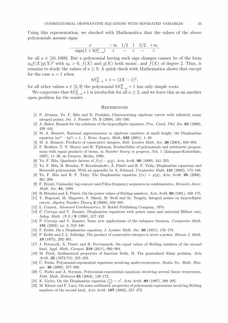
COMBINATORIAL DIOPHANTINE EQUATIONS WITH SEPARATED VARIABLES 25
Using this representation, we checked with Mathematica that the values of the abovepolynomials assume signs
x −∞ 1/2 1 5/2 +∞sign(1 + 8Sxx−a) + − + − +
for all a ∈ [10, 1000]. But a polynomial having such sign changes cannot be of the forma0f(X)g(X)2 with a0 > 0, f(X) and g(X) both monic, and f(X) of degree 2. Thus, itremains to study the values of a ≤ 9. A quick check with Mathematica shows that exceptfor the case a = 1 when
8SXX−1 + 1 = (2X − 1)2,
for all other values a ∈ [2, 9] the polynomial 8SXX−a + 1 has only simple roots.We conjecture that 8SXX−a+1 is irreducible for all a ≥ 2, and we leave this as an another
open problem for the reader.
References
[1] P. Alvanos, Yu. F. Bilu and D. Poulakis, Characterizing algebraic curves with infinitely manyintegral points, Int. J. Number Th. 5 (2009), 585–590.
[2] A. Baker, Bounds for the solutions of the hyperelliptic equation, Proc. Camb. Phil. Soc. 65 (1969),439–444.
[3] M. A. Bennett, Rational approximation to algebraic numbers of small height: the Diophantineequation |axn − byn| = 1, J. Reine Angew. Math. 535 (2001), 1–49.
[4] M. A. Bennett, Products of consecutive integers, Bull. London Math. Soc. 36 (2004), 683–694.[5] F. Beukers, T. N. Shorey and R. Tijdeman, Irreducibility of polynomials and arithmetic progres-
sions with equal products of terms, in Number theory in progress, Vol. 1 (Zakopane-Koscielisko,1997), 11–26, de Gruyter, Berlin, 1999.
[6] Yu. F. Bilu, Quadratic factors of f(x)− g(y), Acta Arith. 90 (1999), 341–355.[7] Yu. F. Bilu, B. Brindza, P. Kirschenhofer, A. Pinter and R. F. Tichy, Diophantine equations and
Bernoulli polynomials. With an appendix by A. Schinzel, Compositio Math. 131 (2002), 173–188.[8] Yu. F. Bilu and R. F. Tichy, The Diophantine equation f(x) = g(y), Acta Arith. 95 (2000),
261–288.[9] F. Brenti, Unimodal, log-concave and Polya frequency sequences in combinatorics, Memoirs Amer.
Math. Soc. 81, 1989.[10] B. Brindza and A. Pinter, On the power values of Stirling numbers, Acta Arith. 60 (1991), 169–175.[11] Y. Bugeaud, M. Mignotte, S. Siksek, M. Stoll and Sz. Tengely, Integral points on hyperelliptic
curves, Algebra Number Theory 2 (2008), 859–885.[12] L. Comtet, Advanced Combinatorics, D. Reidel Publishing Company, 1974.[13] P. Corvaja and U. Zannier, Diophantine equations with power sums and universal Hilbert sets,
Indag. Math. (N.S.) 9 (1998), 317–332.[14] P. Corvaja and U. Zannier, Some new applications of the subspace theorem, Compositio Math.
131 (2002), no. 3, 319–340.[15] P. Erdos, On a Diophantine equation, J. London Math. Soc. 26 (1951), 176–178.[16] P. Erdos and J. L. Selfridge, The product of consecutive integers is never a power, Illinois J. Math.
19 (1975), 292–301.[17] J. Ferenczik, A. Pinter and B. Porvazsnyik. On equal values of Stirling numbers of the second
kind, Appl. Math. Comput. 218 (2011), 980–984.[18] M. Fried, Arithmetical properties of function fields. II. The generalized Schur problem, Acta
Arith. 25 (1973/74), 225–258.[19] C. Fuchs, Polynomial-exponential equations involving multi-recurrences, Studia Sci. Math. Hun-
gar. 46 (2009), 377–398.[20] C. Fuchs and A. Scremin, Polynomial-exponential equations involving several linear recurrences,
Publ. Math. Debrecen 65 (2004), 149–172.[21] K. Gyory, On the Diophantine equation
(nk
)= xl, Acta Arith. 80 (1997), 289–295.
[22] M. Klazar and F. Luca, On some arithmetic properties of polynomial expressions involving Stirlingnumbers of the second kind, Acta Arith. 107 (2003), 357–372.
26 YU.F. BILU, C. FUCHS , F. LUCA, AND A. PINTER
[23] D. W. Masser, Polynomial bounds for diophantine equations, Amer. Math. Monthly 93 (1986),486–488.
[24] M. Mignotte, A note on the equation axn − byn = c, Acta Arith. 75 (1996), 287–295.[25] A. Pinter, On a Diophantine problem concerning Stirling numbers, Acta Math. Hungar. 65 (1994),
361–364.[26] D. Poulakis, A simple method for solving the diophantine equation Y 2 = X4+aX3+bX2+cX+d,
Elem. Math. 54 (1999), 32–36.[27] J. B. Rosser and L. Schoenfeld, Approximate formulas for some functions of prime numbers, Illinois
J. Math. 6 (1962), 64–94.[28] W. M. Schmidt, Diophantine approximations and Diophantine equations, Lecture Notes in Ma-
thematics 1467, Springer-Verlag, Berlin, 1991.[29] T. N. Shorey and R. Tijdeman, Exponential diophantine equations, Cambridge Tracts in Mathe-
matics 87, Cambridge University Press, Cambridge, 1986.[30] Th. Stoll, R. F. Tichy, The Diophantine equation α
(xm
)+ β
(yn
)= γ, Publ. Math. Debrecen 64
(2004), 155–165.[31] R. J. Stroeker and B. M. M. de Weger, Elliptic binomial Diophantine equations, Math. Comp. 68
(1999), 1257–1281.[32] G. Turnwald, On Schur’s conjecture, J. Austral. Math. Soc. 58 (1995), 312–357.[33] P. G. Walsh, A quantitative version of Runge’s theorem on Diophantine equations, Acta Arith.
62 (1992), 157–172; Correction to: A quantitative version of Runge’s theorem on Diophantineequations, Acta Arith. 73 (1995), 397–398.
Yuri F. BiluIMBUniversite Bordeaux 1351 cours de la Libration33405 TalenceFranceEmail: [email protected]
Clemens FuchsDepartment of MathematicsETH ZurichRamistrasse 1018092 ZurichSwitzerlandEmail: [email protected]
Florian LucaMathematical InstituteUNAMAp. Postal 61-3 (Xangari)CP 58 089 Morelia, MichoacanMexicoEmail: [email protected]
Akos PinterInstitute of Mathematics, MTA-DE Research Group ”Equations, Functions and Curves”Hungarian Academy of Sciences and University of DebrecenP. O. Box 12, H-4010 Debrecen, HungaryEmail: [email protected]