Embed Size (px)
Citation preview
COMBINATORICS OF KP SOLITONS FROM THE REAL GRASSMANNIAN
YUJI KODAMA AND LAUREN WILLIAMS
Abstract. Given a point A in the real Grassmannian, it is well-known that one can construct asoliton solution uA(x, y, t) to the KP equation. The contour plot of such a solution provides a tropicalapproximation to the solution when the variables x, y, and t are considered on a large scale and thetime t is fixed. In this paper we give an overview of our work on the combinatorics of such contourplots. Using the positroid stratification and the Deodhar decomposition of the Grassmannian (and inparticular the combinatorics of Go-diagrams), we completely describe the asymptotics of these contourplots when y or t go to ±∞. Other highlights include: a surprising connection with total positivity andcluster algebras; results on the inverse problem; and the characterization of regular soliton solutions– that is, a soliton solution uA(x, y, t) is regular for all times t if and only if A comes from the totally
non-negative part of the Grassmannian.
とき超えて碁石が証す波文様
Arrangements of stonesreveal patterns in the wavesas space-time expands K.W.
Contents
1. Introduction 12. Background on the Grassmannian and its totally non-negative part 33. A Deodhar decomposition of the Grassmannian 64. Deodhar components in the Grassmannian and Go-diagrams 95. Soliton solutions to the KP equation and their contour plots 126. Unbounded line-solitons at y ≫ 0 and y ≪ 0 157. Soliton graphs and generalized plabic graphs 178. The contour plot for t≪ 0 189. Total positivity, regularity, and cluster algebras 2110. The inverse problem for soliton graphs 25References 26
1. Introduction
The main purpose of this paper is to give an exposition of our recent work [18, 19, 20], which foundsurprising connections between soliton solutions of the KP equation and the combinatorics of the realGrassmannian. The KP equation is a two-dimensional nonlinear dispersive wave equation which wasproposed by Kadomtsev and Peviashvili in 1970 to study the stability problem of the soliton solutionof the Korteweg-de Vries (KdV) equation [13]. The equation has a rich mathematical structure, and is
Date: May 4, 2012.The first author was partially supported by NSF grants DMS-0806219 and DMS-1108813. The second author was
partially supported by an NSF CAREER award and an Alfred Sloan Fellowship.
1
2 YUJI KODAMA AND LAUREN WILLIAMS
now considered to be the prototype of an integrable nonlinear dispersive wave equation with two spatialdimensions (see for example [24, 1, 9, 23, 12]). The KP equation can also be used to describe shallowwater wave phenomena, including resonant interactions.
An important breakthrough in the KP theory was made by Sato [26], who realized that solutionsof the KP equation could be written in terms of points on an infinite-dimensional Grassmannian. Thepresent paper, which gives an overview of most of our results of [19] and [20], deals with a real, finite-dimensional version of the Sato theory. In particular, we are interested in soliton solutions, that is,solutions that are localized along certain rays in the xy plane called line-solitons. Such a solution canbe constructed from a point A of the real Grassmannian. More specifically, one can apply the Wronskianform [26, 27, 11, 12] to A to produce a certain sum of exponentials called a τ-function τA(x, y, t), andfrom the τ -function one can construct a solution uA(x, y, t) to the KP equation.
Recently several authors have studied the soliton solutions uA(x, y, t) which come from points A of thetotally non-negative part of the Grassmannian (Grk,n)≥0, that is, those points of the real GrassmannianGrk,n whose Plucker coordinates are all non-negative [3, 16, 2, 5, 7, 18, 19]. These solutions are regular,and include a large variety of soliton solutions which were previously overlooked by those using theHirota method of a perturbation expansion [12].
A main goal of [20] was to understand the soliton solutions uA(x, y, t) coming from arbitrary points Aof the real Grassmannian, not just the totally non-negative part. In general such solutions are no longerregular – they may have singularities along rays in the xy plane – but it is possible, nevertheless, tounderstand a great deal about the asymptotics of such solutions, when the absolute value of the spatialvariable y goes to infinity, and also when the absolute value of the time variable t goes to infinity.
Two related decompositions of the real Grassmannian are useful for understanding the asymptoticsof soliton solutions uA(x, y, t). The first is Postnikov’s positroid stratification of the Grassmannian [25],whose strata are indexed by various combinatorial objects including decorated permutations and
Γ-
diagrams. This decomposition determines the asympototics of soliton solutions when |y| ≫ 0, and ourresults here extend work of [2, 5, 7, 18, 19] from the setting of the non-negative part of the Grassmannianto the entire real Grassmannian. The second decomposition, which we call the Deodhar decomposition[20], is the projection to the Grassmannian of a decomposition of the flag variety due to Deodhar.The Deodhar decomposition refines the positroid stratification, and its components may be indexed bycertain tableaux filled with black and white stones called Go-diagrams, which generalize
Γ
-diagrams.This decomposition determines the asymptotics of soliton solutions when |t| ≫ 0. More specifically, itallows us to compute the contour plots at |t| ≫ 0 of such solitons, which are tropical approximationsto the solution when x, y, and t are on a large scale [20].
By using our results on the asymptotics of soliton solutions when t≪ 0, one may give a characteri-zation of the regular soliton solutions coming from the real Grassmannian. More specifically, a solitonsolution uA(x, y, t) coming from a point A of the real Grassmannian is regular for all times t if and onlyif A is a point of the totally non-negative part of the Grassmannian [20].
The regularity theorem above provides an important motivation for studying soliton solutions comingfrom (Grk,n)≥0. Indeed, as we showed in [19], such soliton solutions have an even richer combinatorialstructure than those coming from Grk,n. For example, (generic) contour plots coming from the totallypositive part (Grk,n)>0 of the Grassmannian give rise to clusters for the cluster algebra associated tothe Grassmannian. And up to a combinatorial equivalence, the contour plots coming from (Gr2,n)>0
are in bijection with triangulations of an n-gon. Finally, if either A ∈ (Grk,n)>0, or A ∈ (Grk,n)≥0 andt ≪ 0, then one may solve the inverse problem for uA(x, y, t): that is, given the contour plot Ct(uA)and the time t, one may reconstruct the element A ∈ (Grk,n)≥0. And therefore one may reconstructthe entire evolution of this soliton solution over time [19].
The structure of this paper is as follows. In Section 2 we provide background on the Grassmannianand some of its decompositions, including the positroid stratification. In Section 3 we describe the
COMBINATORICS OF KP SOLITONS FROM THE REAL GRASSMANNIAN 3
Deodhar decomposition of the complete flag variety and its projection to the Grassmannian, whilein Section 4 we explain how to index Deodhar components in the Grassmannian by Go-diagrams.Subsequent sections provide applications of the previous results to soliton solutions of the KP equation.In Section 5 we explain how to produce a soliton solution to the KP equation from a point of the realGrassmannian, and then define the contour plot associated to a soliton solution at a fixed time t. InSection 6 we use the positroid stratification to describe the unbounded line-solitons in contour plots ofsoliton solutions at y ≫ 0 and y ≪ 0. In Section 7 we define the more combinatorial notions of solitongraph and generalized plabic graph. In Section 8 we use the Deodhar decomposition to describe contourplots of soliton solutions for t≪ 0. In Section 9 we describe the significance of total positivity to solitonsolutions, by discussing the regularity problem, as well as the connection to cluster algebras. Finally inSection 10, we give results on the inverse problem for soliton solutions coming from (Grk,n)≥0.
2. Background on the Grassmannian and its totally non-negative part
The real Grassmannian Grk,n is the space of all k-dimensional subspaces of Rn. An element of Grk,n
can be viewed as a full-rank k× n matrix modulo left multiplication by nonsingular k× k matrices. Inother words, two k × n matrices represent the same point in Grk,n if and only if they can be obtained
from each other by row operations. Let(
[n]k
)
be the set of all k-element subsets of [n] := 1, . . . , n. For
I ∈(
[n]k
)
, let ∆I(A) be the Plucker coordinate, that is, the maximal minor of the k×n matrix A located
in the column set I. The map A 7→ (∆I(A)), where I ranges over(
[n]k
)
, induces the Plucker embedding
Grk,n → RP(n
k)−1. The totally non-negative part of the Grassmannian (Grk,n)≥0 is the subset of Grk,n
such that all Plucker coordinates are non-negative.We now describe several useful decompositions of the Grassmannian: the matroid stratification, the
Schubert decomposition, and the positroid stratification. When one restricts the positroid stratificationto (Grk,n)≥0, one gets a cell decomposition of (Grk,n)≥0 into positroid cells.
2.1. The matroid stratification of Grk,n.
Definition 2.1. A matroid of rank k on the set [n] is a nonempty collection M ⊂(
[n]k
)
of k-elementsubsets in [n], called bases ofM, that satisfies the exchange axiom:For any I, J ∈M and i ∈ I there exists j ∈ J such that (I \ i) ∪ j ∈ M.
Given an element A ∈ Grk,n, there is an associated matroid MA whose bases are the k-subsetsI ⊂ [n] such that ∆I(A) 6= 0.
Definition 2.2. Let M⊂(
[n]k
)
be a matroid. The matroid stratum SM is defined to be
SM = A ∈ Grk,n | ∆I(A) 6= 0 if and only if I ∈ M.
This gives a stratification of Grk,n called the matroid stratification, or Gelfand-Serganova stratification.The matroidsM with nonempty strata SM are called realizable over R.
2.2. The Schubert decomposition of Grk,n. Recall that the partitions λ ⊂ (n−k)k are in bijectionwith k-element subset I ⊂ [n]. The boundary of the Young diagram of such a partition λ forms a latticepath from the upper-right corner to the lower-left corner of the rectangle (n− k)k. Let us label the nsteps in this path by the numbers 1, . . . , n, and define I = I(λ) as the set of labels on the k verticalsteps in the path. Conversely, we let λ(I) denote the partition corresponding to the subset I.
Definition 2.3. For each partition λ ⊂ (n− k)k, one can define the Schubert cell Ωλ by
Ωλ = A ∈ Grk,n | I(λ) is the lexicographically minimal base of MA.
4 YUJI KODAMA AND LAUREN WILLIAMS
As λ ranges over the partitions contained in (n − k)k, this gives the Schubert decomposition of theGrassmannian Grk,n, i.e.
Grk,n =⊔
λ⊂(n−k)k
Ωλ.
We now define the shifted linear order <i (for i ∈ [n]) to be the total order on [n] defined by
i <i i + 1 <i i + 2 <i · · · <i n <i 1 <i · · · <i i− 1.
One can then define cyclically shifted Schubert cells as follows.
Definition 2.4. For each partition λ ⊂ (n− k)k and i ∈ [n], the cyclically shifted Schubert cell Ωiλ is
Ωiλ = A ∈ Grk,n | I(λ) is the lexicographically minimal base of MA with respect to <i.
2.3. The positroid stratification of Grk,n. The positroid stratification of the real GrassmannianGrk,n is obtained by taking the simultaneous refinement of the n Schubert decompositions with respectto the n shifted linear orders <i. This stratification was first considered by Postnikov [25], who showedthat the strata are conveniently described in terms of Grassmann necklaces, as well as decorated per-mutations, (equivalence classes of) plabic graphs, and
Γ
-diagrams. Postnikov coined the terminologypositroid because the intersection of the positroid stratification with (Grk,n)≥0 gives a cell decomposi-tion of (Grk,n)≥0 (whose cells are called positroid cells).
Definition 2.5. [25, Definition 16.1] A Grassmann necklace is a sequence I = (I1, . . . , In) of subsetsIr ⊂ [n] such that, for i ∈ [n], if i ∈ Ii then Ii+1 = (Ii \ i) ∪ j, for some j ∈ [n]; and if i /∈ Ir thenIi+1 = Ii. (Here indices i are taken modulo n.) In particular, we have |I1| = · · · = |In|, which is equalto some k ∈ [n]. We then say that I is a Grassmann necklace of type (k, n).
Example 2.6. (1257, 2357, 3457, 4567, 5678, 6789, 1789, 1289, 1259) is a Grassmann necklace of type (4, 9).
Lemma 2.7. [25, Lemma 16.3] Given A ∈ Grk,n, let I(A) = (I1, . . . , In) be the sequence of subsets in
[n] such that, for i ∈ [n], Ii is the lexicographically minimal subset of(
[n]k
)
with respect to the shiftedlinear order <i such that ∆Ii
(A) 6= 0. Then I(A) is a Grassmann necklace of type (k, n).
If A is in the matroid stratum SM, we also use IM to denote the sequence (I1, . . . , In) defined above.This leads to the following description of the positroid stratification of Grk,n.
Definition 2.8. Let I = (I1, . . . , In) be a Grassmann necklace of type (k, n). The positroid stratum SI
is defined to be
SI = A ∈ Grk,n | I(A) = I
=n⋂
i=1
Ωiλ(Ii)
.
The second equality follows from Definition 2.8 and Definition 2.4. Note that each positroid stratumis an intersection of n cyclically shifted Schubert cells.
Definition 2.9. [25, Definition 13.3] A decorated permutation π: = (π, col) is a permutation π ∈ Sn
together with a coloring function col from the set of fixed points i | π(i) = i to 1,−1. So a decoratedpermutation is a permutation with fixed points colored in one of two colors. A weak excedance of π: isa pair (i, πi) such that either π(i) > i, or π(i) = i and col(i) = 1. We call i the weak excedance position.If π(i) > i (respectively π(i) < i) then (i, πi) is called an excedance (respectively, nonexcedance).
Example 2.10. The decorated permutation (written in one-line notation) (6, 7, 1, 2, 8, 3, 9, 4, 5) has nofixed points, and four weak excedances, in positions 1, 2, 5 and 7.
COMBINATORICS OF KP SOLITONS FROM THE REAL GRASSMANNIAN 5
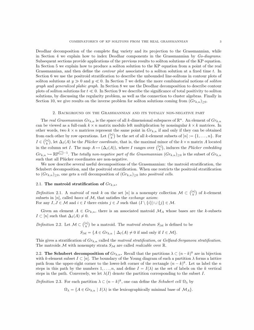
Definition 2.11. A plabic graph is a planar undirected graph G drawn inside a disk with n boundaryvertices 1, . . . , n placed in counterclockwise order around the boundary of the disk, such that eachboundary vertex i is incident to a single edge.1 Each internal vertex is colored black or white. See theleft of Figure 1 for an example.
Definition 2.12. [25, Definition 6.1] Fix k, n. If λ is a partition, let Yλ denote its Young diagram. A
Γ
-diagram (λ, D)k,n of type (k, n) is a partition λ contained in a k × (n− k) rectangle together with afilling D : Yλ → 0, + which has the
Γ
-property: there is no 0 which has a + above it and a + to itsleft.2 (Here, “above” means above and in the same column, and “to its left” means to the left and inthe same row.) See the right of Figure 1 for an example.
1 2
34
5
+ +
+ +
+
+
+
+
+
+ + + ++
+ + + +
+ +
0
0 0 0 0 0 0 0 00 0 0 0 0 0
000 00
0 0 0
k
n - k
λ = (10, 9, 9, 8, 5, 2)
k = 6, n = 16
Figure 1. A plabic graph and a Le-diagram L = (λ, D)k,n.
We now review some of the bijections among these objects.
Definition 2.13. [25, Section 16] Given a Grassmann necklace I, define a decorated permutation π: =π:(I) by requiring that
(1) if Ii+1 = (Ii \ i) ∪ j, for j 6= i, then π:(j) = i. 3
(2) if Ii+1 = Ii and i ∈ Ii then π(i) = i is colored with col(i) = 1.(3) if Ii+1 = Ii and i /∈ Ii then π(i) = i is colored with col(i) = −1.
As before, indices are taken modulo n.
If π: = π:(I), then we also use the notation Sπ: to refer to the positroid stratum SI .
Example 2.14. Definition 2.13 carries the Grassmann necklace of Example 2.6 to the decorated permu-tation of Example 2.10.
Lemma 2.15. [25, Lemma 16.2] The map I → π:(I) is a bijection from Grassmann necklaces I =(I1, . . . , In) of size n to decorated permutations π:(I) of size n. Under this bijection, the weak excedancesof π:(I) are in positions I1.
One particularly nice class of positroid cells is the TP or totally positive Schubert cells.
Definition 2.16. A totally positive Schubert cell is the intersection of a Schubert cell with (Grk,n)≥0.
TP Schubert cells are indexed by
Γ
-diagrams such that all boxes are filled with a +.
1The convention of [25] was to place the boundary vertices in clockwise order.2This forbidden pattern is in the shape of a backwards L, and hence is denoted
Γ
and pronounced “Le.”3Actually Postnikov’s convention was to set π:(i) = j above, so the decorated permutation we are associating is the
inverse one to his.
6 YUJI KODAMA AND LAUREN WILLIAMS
3. A Deodhar decomposition of the Grassmannian
In this section we review Deodhar’s decomposition of the flag variety G/B [8], and the parameteriza-tions of the components due to Marsh and Rietsch [22]. We then give a Deodhar decomposition of theGrassmannian by projecting the usual Deodhar decomposition of the flag variety to the Grassmannian.
3.1. The flag variety. In this paper we fix the group G = SLn = SLn(R), a maximal torus T , andopposite Borel subgroups B+ and B−, which consist of the diagonal, upper-triangular, and lower-triangular matrices, respectively. We let U+ and U− be the unipotent radicals of B+ and B−; theseare the subgroups of upper-triangular and lower-triangular matrices with 1’s on the diagonals. For each1 ≤ i ≤ n− 1 we have a homomorphism φi : SL2 → SLn such that
φi
(
a bc d
)
=
1. . .
a bc d
. . .
1
∈ SLn,
that is, φi replaces a 2 × 2 block of the identity matrix with
(
a bc d
)
. Here a is at the (i + 1)st
diagonal entry counting from the southeast corner.4 We use this to construct 1-parameter subgroupsin G (landing in U+ and U−, respectively) defined by
xi(m) = φi
(
1 m0 1
)
and yi(m) = φi
(
1 0m 1
)
, where m ∈ R.
Let W denote the Weyl group NG(T )/T , where NG(T ) is the normalizer of T . The simple reflections
si ∈ W are given explicitly by si := siT where si := φi
(
0 −11 0
)
and any w ∈ W can be expressed
as a product w = si1si2 . . . simwith m = ℓ(w) factors. We set w = si1 si2 . . . sim
. For G = SLn, we haveW = Sn, the symmetric group on n letters, and si is the transposition exchanging i and i + 1.
We can identify the flag variety G/B with the variety B of Borel subgroups, via
gB ←→ g ·B+ := gB+g−1.
We have two opposite Bruhat decompositions of B:
B =⊔
w∈W
B+w · B+ =⊔
v∈W
B−v ·B+.
We define the Richardson variety
Rv,w := B+w ·B+ ∩B−v ·B+,
the intersection of opposite Bruhat cells. This intersection is empty unless v ≤ w, in which case it issmooth of dimension ℓ(w) − ℓ(v), see [15, 21].
4Our numbering differs from that in [22] in that the rows of our matrices in SLn are numbered from the bottom.
COMBINATORICS OF KP SOLITONS FROM THE REAL GRASSMANNIAN 7
3.2. Distinguished expressions. We now provide background on distinguished and positive distin-guished subexpressions, as in [8] and [22]. We will assume that the reader is familiar with the (strong)Bruhat order < on the Weyl group W = Sn, and the basics of reduced expressions, as in [4].
Let w := si1 . . . simbe a reduced expression for w ∈ W . A subexpression v of w is a word obtained
from the reduced expression w by replacing some of the factors with 1. For example, consider a reducedexpression in S4, say s3s2s1s3s2s3. Then s3s2 1 s3s2 1 is a subexpression of s3s2s1s3s2s3. Given asubexpression v, we set v(k) to be the product of the leftmost k factors of v, if k ≥ 1, and v(0) = 1.
Definition 3.1. [22, 8] Given a subexpression v of a reduced expression w = si1si2 . . . sim, we define
Jv
:= k ∈ 1, . . . , m | v(k−1) < v(k),
J
v:= k ∈ 1, . . . , m | v(k−1) = v(k),
J•v
:= k ∈ 1, . . . , m | v(k−1) > v(k).
The expression v is called non-decreasing if v(j−1) ≤ v(j) for all j = 1, . . . , m, e.g. J•v
= ∅.
Definition 3.2 (Distinguished subexpressions). [8, Definition 2.3] A subexpression v of w is calleddistinguished if we have
(3.1) v(j) ≤ v(j−1) sijfor all j ∈ 1, . . . , m.
In other words, if right multiplication by sijdecreases the length of v(j−1), then in a distinguished
subexpression we must have v(j) = v(j−1)sij.
We write v ≺ w if v is a distinguished subexpression of w.
Definition 3.3 (Positive distinguished subexpressions). We call a subexpression v of w a positive dis-tinguished subexpression (or a PDS for short) if
(3.2) v(j−1) < v(j−1)sijfor all j ∈ 1, . . . , m.
In other words, it is distinguished and non-decreasing.
Lemma 3.4. [22] Given v ≤ w and a reduced expression w for w, there is a unique PDS v+ for v in w.
3.3. Deodhar components in the flag variety. We now describe the Deodhar decomposition of theflag variety. This is a further refinement of the decomposition of G/B into Richardson varieties Rv,w.Marsh and Rietsch [22] gave explicit parameterizations for each Deodhar component, identifying eachone with a subset in the group.
Definition 3.5. [22, Definition 5.1] Let w = si1 . . . simbe a reduced expression for w, and let v be a
distinguished subexpression. Define a subset Gv,w in G by
(3.3) Gv,w :=
g = g1g2 · · · gm
∣
∣
∣
∣
∣
∣
gℓ = xiℓ(mℓ)s
−1iℓ
if ℓ ∈ J•v,
gℓ = yiℓ(pℓ) if ℓ ∈ J
v,
gℓ = siℓif ℓ ∈ J
v,
for pℓ ∈ R∗, mℓ ∈ R.
.
There is an obvious map (R∗)|Jv| × R|J•
v| → Gv,w defined by the parameters pℓ and mℓ in (3.3). For
v = w = 1 we define Gv,w = 1.
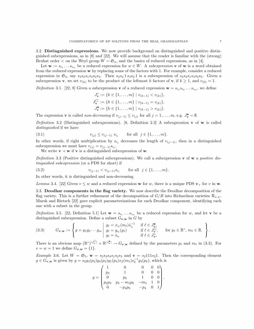
Example 3.6. Let W = S5, w = s2s3s4s1s2s3 and v = s2111s21. Then the corresponding elementg ∈ Gv,w is given by g = s2y3(p2)y4(p3)y1(p4)x2(m5)s
−12 y3(p6), which is
g =
1 0 0 0 0p3 1 0 0 00 p6 1 0 0
p2p3 p2 −m5p6 −m5 1 00 −p4p6 −p4 0 1
.
8 YUJI KODAMA AND LAUREN WILLIAMS
The following result from [22] gives an explicit parametrization for the Deodhar component Rv,w.We will take the description below as the definition of Rv,w.
Proposition 3.7. [22, Proposition 5.2] The map (R∗)|Jv| × R|J•
v| → Gv,w from Definition 3.5 is an
isomorphism. The set Gv,w lies in U−v∩B+wB+, and the assignment g 7→ g·B+ defines an isomorphism
Gv,w∼−→ Rv,w(3.4)
between the subset Gv,w of the group, and the Deodhar component Rv,w in the flag variety.
Suppose that for each w ∈W we choose a reduced expression w for w. Then it follows from Deodhar’swork (see [8] and [22, Section 4.4]) that
(3.5) Rv,w =⊔
v≺w
Rv,w and G/B =⊔
w∈W
(
⊔
v≺w
Rv,w
)
.
These are called the Deodhar decompositions of Rv,w and G/B.
Remark 3.8. One may define the Richardson variety Rv,w over a finite field Fq. In this setting thenumber of points determine the R-polynomials Rv,w(q) = #(Rv,w(Fq)) introduced by Kazhdan andLusztig [14] to give a formula for the Kazhdan-Lusztig polynomials. This was the original motivation for
Deodhar’s work. Therefore the isomorphisms Rv,w∼= (F∗
q)|J
v × F|J•
v|
q together with the decomposition(3.5) give formulas for the R-polynomials.
3.4. Projections of Deodhar components to the Grassmannian. Now we consider the projec-tion of the Deodhar decomposition to the Grassmannian Grk,n. Let Wk be the parabolic subgroup〈s1, s2, . . . , sn−k, . . . , sn−1〉 of W = Sn, and let W k denote the set of minimal-length coset represen-tatives of W/Wk. Recall that a descent of a permutation π is a position j such that π(j) > π(j + 1).Then W k is the subset of permutations of Sn which have at most one descent; and that descent mustbe in position n− k.
Let πk : G/B → Grk,n be the projection from the flag variety to the Grassmannian. For eachw ∈ W k and v ≤ w, define Pv,w = πk(Rv,w). Then by work of Lusztig [21], πk is an isomorphism onPv,w, and we have a decomposition
(3.6) Grk,n =⊔
w∈W k
⊔
v≤w
Pv,w
.
Definition 3.9. For each reduced decomposition w for w ∈ W k, and each v ≺ w, we define the(projected) Deodhar component Pv,w = πk(Rv,w) ⊂ Grk,n.
Lemma 3.10. [20, Remark 3.12, Lemma 3.13] The decomposition in (3.6) coincides with the positroidstratification from Section 2.3. The appropriate bijection between the strata is defined as follows. LetQk denote the set of pairs (v, w) where v ∈W , w ∈W k, and v ≤ w; let Deck
n denote the set of decoratedpermutations in Sn with k weak excedances. We consider both sets as partially ordered sets, wherethe cover relation corresponds to containment of closures of the corresponding strata. Then there isan order-preserving bijection Φ from Qk to Deck
n which is defined as follows. Let (v, w) ∈ QJ . ThenΦ(v, w) = (π, col) where π = vw−1. We also let π:(v, w) denote Φ(v, w). To define col, we color anyfixed point that occurs in one of the positions w(1), w(2), . . . , w(n−k) with the color −1, and color anyother fixed point with the color 1.
By Lemma 3.10, Pv,w lies in the positroid stratum Sπ: . Note that the strata Pv,w do not depend onthe chosen reduced decomposition of w [19, Proposition 4.16].
COMBINATORICS OF KP SOLITONS FROM THE REAL GRASSMANNIAN 9
Now if for each w ∈ W k we choose a reduced decomposition w, then we have
(3.7) Pv,w =⊔
v≺w
Pv,w and Grk,n =⊔
w∈W k
(
⊔
v≺w
Pv,w
)
.
Proposition 3.7 gives us a concrete way to think about the projected Deodhar components Pv,w.The projection πk : G/B → Grk,n maps each g ∈ Gv,w to the span of its leftmost k columns:
g =
gn,n . . . gn,n−k+1 . . . gn,1
......
...g1,n . . . g1,n−k+1 . . . g1,1
7→ A =
g1,n−k+1 . . . gn,n−k+1
......
g1,n . . . gn,n
.
Alternatively, we may identify A ∈ Grk,n with its image in the Plucker embedding. Let ei denote thecolumn vector in Rn such that the ith entry from the bottom contains a 1, and all other entries are 0,e.g. en = (1, 0, . . . , 0)T , the transpose of the row vector (1, 0, . . . , 0). Then the projection πk maps eachg ∈ Gv,w (identified with g · B+ ∈ Rv,w) to
g · en ∧ . . . ∧ en−k+1 =∑
1≤j1<...<jk≤n
∆j1,...,jk(A)ejk
∧ · · · ∧ ej1 .(3.8)
That is, the Plucker coordinate ∆j1,...,jk(A) is given by
∆j1,...,jk(A) = 〈ejk
∧ · · · ∧ ej1 , g · en ∧ · · · ∧ en−k+1〉,
where 〈·, ·〉 is the usual inner product on ∧kRn.
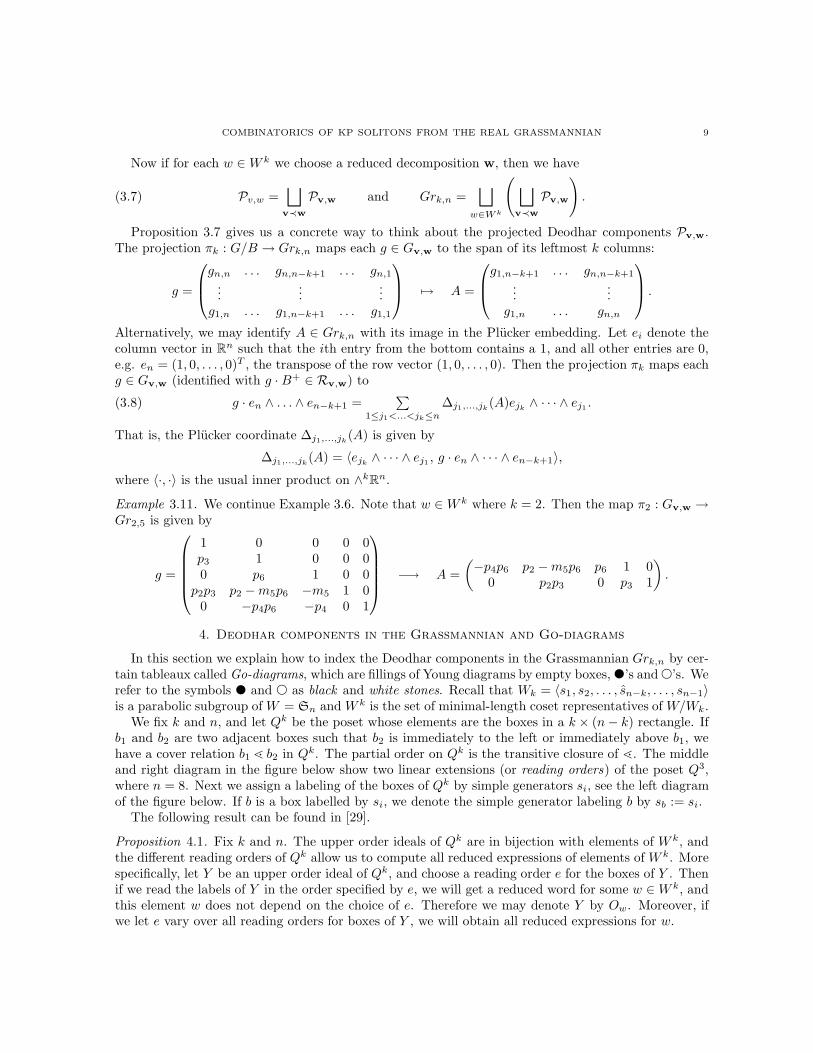
Example 3.11. We continue Example 3.6. Note that w ∈ W k where k = 2. Then the map π2 : Gv,w →Gr2,5 is given by
g =
1 0 0 0 0p3 1 0 0 00 p6 1 0 0
p2p3 p2 −m5p6 −m5 1 00 −p4p6 −p4 0 1
−→ A =
(
−p4p6 p2 −m5p6 p6 1 00 p2p3 0 p3 1
)
.
4. Deodhar components in the Grassmannian and Go-diagrams
In this section we explain how to index the Deodhar components in the Grassmannian Grk,n by cer-tain tableaux called Go-diagrams, which are fillings of Young diagrams by empty boxes, ’s and ’s. Werefer to the symbols and as black and white stones. Recall that Wk = 〈s1, s2, . . . , sn−k, . . . , sn−1〉is a parabolic subgroup of W = Sn and W k is the set of minimal-length coset representatives of W/Wk.
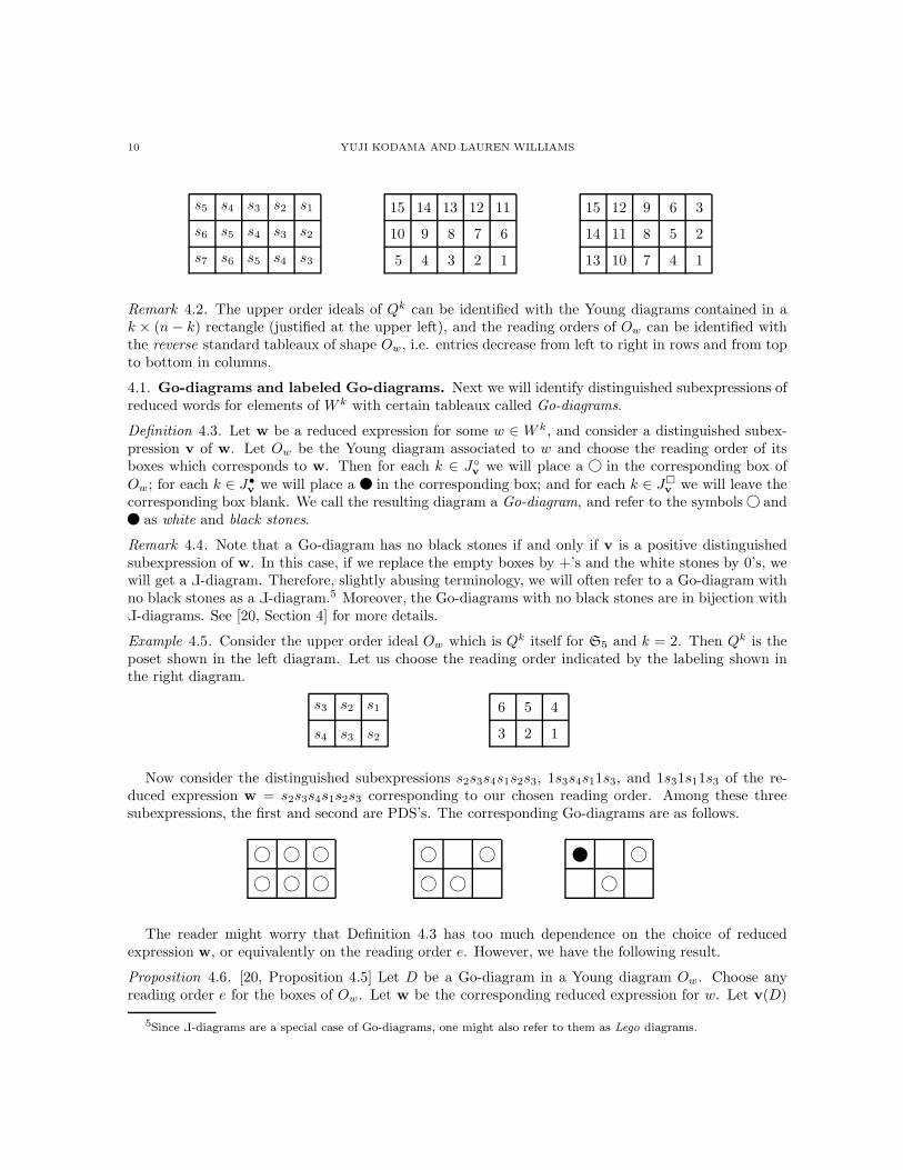
We fix k and n, and let Qk be the poset whose elements are the boxes in a k × (n− k) rectangle. Ifb1 and b2 are two adjacent boxes such that b2 is immediately to the left or immediately above b1, wehave a cover relation b1 ⋖ b2 in Qk. The partial order on Qk is the transitive closure of ⋖. The middleand right diagram in the figure below show two linear extensions (or reading orders) of the poset Q3,where n = 8. Next we assign a labeling of the boxes of Qk by simple generators si, see the left diagramof the figure below. If b is a box labelled by si, we denote the simple generator labeling b by sb := si.
The following result can be found in [29].
Proposition 4.1. Fix k and n. The upper order ideals of Qk are in bijection with elements of W k, andthe different reading orders of Qk allow us to compute all reduced expressions of elements of W k. Morespecifically, let Y be an upper order ideal of Qk, and choose a reading order e for the boxes of Y . Thenif we read the labels of Y in the order specified by e, we will get a reduced word for some w ∈W k, andthis element w does not depend on the choice of e. Therefore we may denote Y by Ow. Moreover, ifwe let e vary over all reading orders for boxes of Y , we will obtain all reduced expressions for w.
10 YUJI KODAMA AND LAUREN WILLIAMS
s5 s4 s3 s2 s1
s6 s5 s4 s3 s2
s7 s6 s5 s4 s3
15 14 13 12 11
10 9 8 7 6
5 4 3 2 1
15 12 9 6 3
14 11 8 5 2
13 10 7 4 1
Remark 4.2. The upper order ideals of Qk can be identified with the Young diagrams contained in ak × (n− k) rectangle (justified at the upper left), and the reading orders of Ow can be identified withthe reverse standard tableaux of shape Ow, i.e. entries decrease from left to right in rows and from topto bottom in columns.
4.1. Go-diagrams and labeled Go-diagrams. Next we will identify distinguished subexpressions ofreduced words for elements of W k with certain tableaux called Go-diagrams.
Definition 4.3. Let w be a reduced expression for some w ∈ W k, and consider a distinguished subex-pression v of w. Let Ow be the Young diagram associated to w and choose the reading order of itsboxes which corresponds to w. Then for each k ∈ J
vwe will place a in the corresponding box of
Ow; for each k ∈ J•v
we will place a in the corresponding box; and for each k ∈ Jv
we will leave thecorresponding box blank. We call the resulting diagram a Go-diagram, and refer to the symbols andas white and black stones.
Remark 4.4. Note that a Go-diagram has no black stones if and only if v is a positive distinguishedsubexpression of w. In this case, if we replace the empty boxes by +’s and the white stones by 0’s, wewill get a
Γ-diagram. Therefore, slightly abusing terminology, we will often refer to a Go-diagram with
no black stones as a
Γ
-diagram.5 Moreover, the Go-diagrams with no black stones are in bijection with
Γ
-diagrams. See [20, Section 4] for more details.
Example 4.5. Consider the upper order ideal Ow which is Qk itself for S5 and k = 2. Then Qk is theposet shown in the left diagram. Let us choose the reading order indicated by the labeling shown inthe right diagram.
s3 s2 s1
s4 s3 s2
6 5 4
3 2 1
Now consider the distinguished subexpressions s2s3s4s1s2s3, 1s3s4s11s3, and 1s31s11s3 of the re-duced expression w = s2s3s4s1s2s3 corresponding to our chosen reading order. Among these threesubexpressions, the first and second are PDS’s. The corresponding Go-diagrams are as follows.
②
The reader might worry that Definition 4.3 has too much dependence on the choice of reducedexpression w, or equivalently on the reading order e. However, we have the following result.
Proposition 4.6. [20, Proposition 4.5] Let D be a Go-diagram in a Young diagram Ow. Choose anyreading order e for the boxes of Ow. Let w be the corresponding reduced expression for w. Let v(D)
5Since
Γ
-diagrams are a special case of Go-diagrams, one might also refer to them as Lego diagrams.
COMBINATORICS OF KP SOLITONS FROM THE REAL GRASSMANNIAN 11
be the subexpression of w obtained as follows: if a box b of D contains a black or white stone thenthe corresponding simple generator sb is present in the subexpression, while if b is empty, we omit thecorresonding simple generator. Then we have the following:
(1) the element v := v(D) is independent of the choice of reading word e.(2) whether v(D) is a PDS depends only on D (and not e).(3) whether v(D) is distinguished depends only on D (and not on e).
Definition 4.7. Let Ow be an upper order ideal of Qk, where w ∈ W k and W = Sn. Consider aGo-diagram D of shape Ow; this is contained in a k × (n − k) rectangle, and the shape Ow givesrise to a lattice path from the northeast corner to the southwest corner of the rectangle. Label thesteps of that lattice path from 1 to n; this gives a natural labeling to every row and column of therectangle. We now let v := v(D), and we define π:(D) to be the decorated permutation (π(D), col)where π = π(D) = vw−1. The fixed points of π correspond precisely to rows and columns of therectangle with no +’s. If there are no +’s in the row (respectively, column) labeled by h, then π(h) = hand this fixed point gets colored with color 1 (respectively, −1.)
Remark 4.8. It follows from Lemma 3.10 that the projected Deodhar component PD corresponding toD is contained in the positroid stratum Sπ:(D).
Remark 4.9. Recall from Remark 3.8 that the isomorphisms Rv,w∼= (F∗
q)|J
v × F|J•
v|
q together withthe decomposition (3.5) give formulas for the R-polynomials. Therefore a good characterization ofGo-diagrams could lead to explicit formulas for the corresponding R-polynomials.
If we choose a reading order of Ow , then we will also associate to a Go-diagram of shape Ow a labeledGo-diagram, as defined below. Equivalently, a labeled Go-diagram is associated to a pair (v,w).
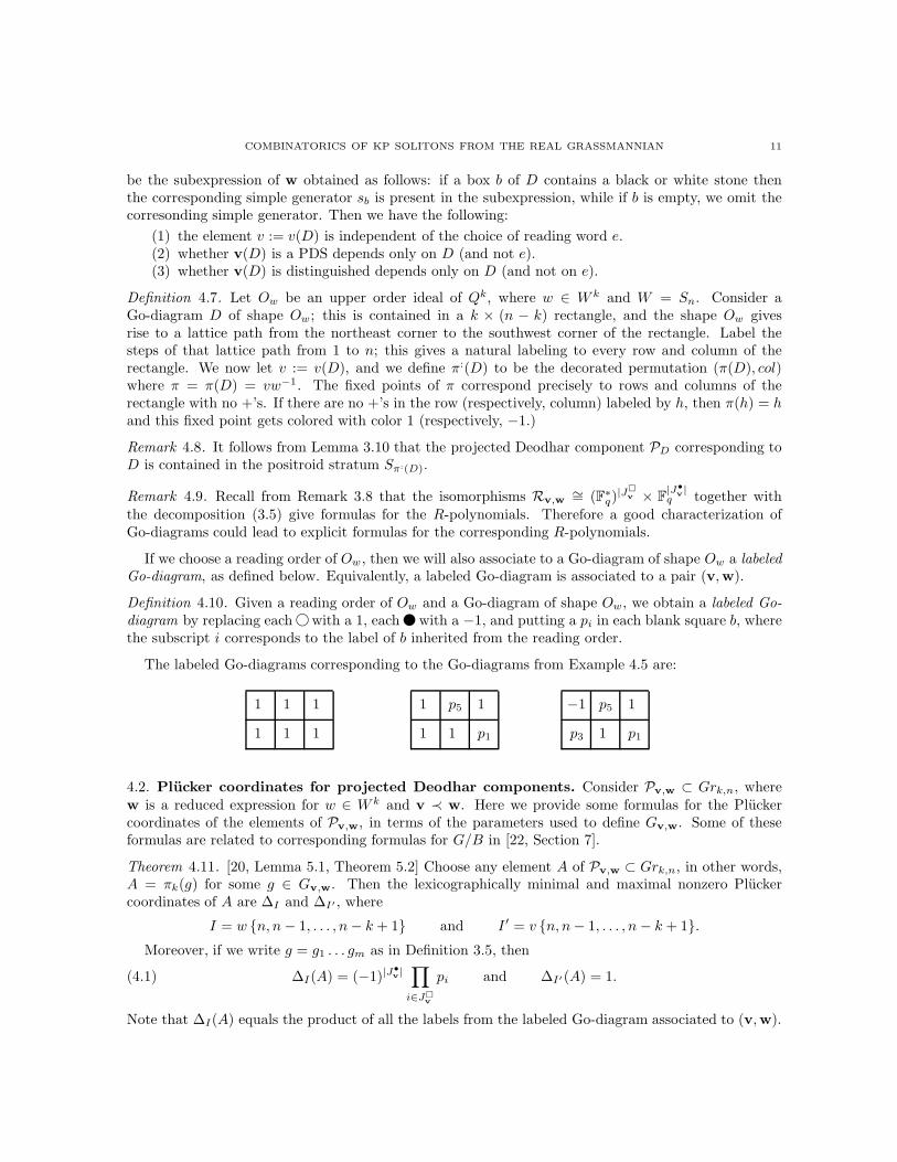
Definition 4.10. Given a reading order of Ow and a Go-diagram of shape Ow, we obtain a labeled Go-diagram by replacing each with a 1, each with a −1, and putting a pi in each blank square b, wherethe subscript i corresponds to the label of b inherited from the reading order.
The labeled Go-diagrams corresponding to the Go-diagrams from Example 4.5 are:
1 1 1
1 1 1
1 p5 1
1 1 p1
−1 p5 1
p3 1 p1
4.2. Plucker coordinates for projected Deodhar components. Consider Pv,w ⊂ Grk,n, wherew is a reduced expression for w ∈ W k and v ≺ w. Here we provide some formulas for the Pluckercoordinates of the elements of Pv,w, in terms of the parameters used to define Gv,w. Some of theseformulas are related to corresponding formulas for G/B in [22, Section 7].
Theorem 4.11. [20, Lemma 5.1, Theorem 5.2] Choose any element A of Pv,w ⊂ Grk,n, in other words,A = πk(g) for some g ∈ Gv,w. Then the lexicographically minimal and maximal nonzero Pluckercoordinates of A are ∆I and ∆I′ , where
I = w n, n− 1, . . . , n− k + 1 and I ′ = v n, n− 1, . . . , n− k + 1.
Moreover, if we write g = g1 . . . gm as in Definition 3.5, then
(4.1) ∆I(A) = (−1)|J•
v|∏
i∈Jv
pi and ∆I′(A) = 1.
Note that ∆I(A) equals the product of all the labels from the labeled Go-diagram associated to (v,w).
12 YUJI KODAMA AND LAUREN WILLIAMS
This theorem can be extended to provide a formula for some other Plucker coordinates. Let b beany box of D. We can choose a linear extension e of the boxes of D which orders the boxes which areweakly southeast of b (the inner boxes) before the rest (the outer boxes). This gives rise to a reducedexpression w and subexpression v, as well as reduced expressions win
b = win, vinb = vin, wout
b = wout,and vout
b = vout, which are obtained by restricting w and v to the inner and outer boxes, respectively.
Theorem 4.12. [20, Theorem 5.6] Let w = si1 . . . simbe a reduced expression for w ∈ W k and v ≺ w,
and let D be the corresponding Go-diagram. Choose any box b of D, and let vin = vinb and win = win
b ,and vout = vout
b and wout = woutb . Let A = πk(g) for any g ∈ Gv,w, and let I = wn, n−1, . . . , n−k+1.
Define Ib = vin(win)−1I ∈(
[n]k
)
. If we write g = g1 . . . gm as in Definition 3.5, then
(4.2) ∆Ib(A) = (−1)|J
•
vout |
∏
i∈J
vout
pi.
Note that ∆Ib(A) equals the product of all the labels in the “out” boxes of the labeled Go-diagram.
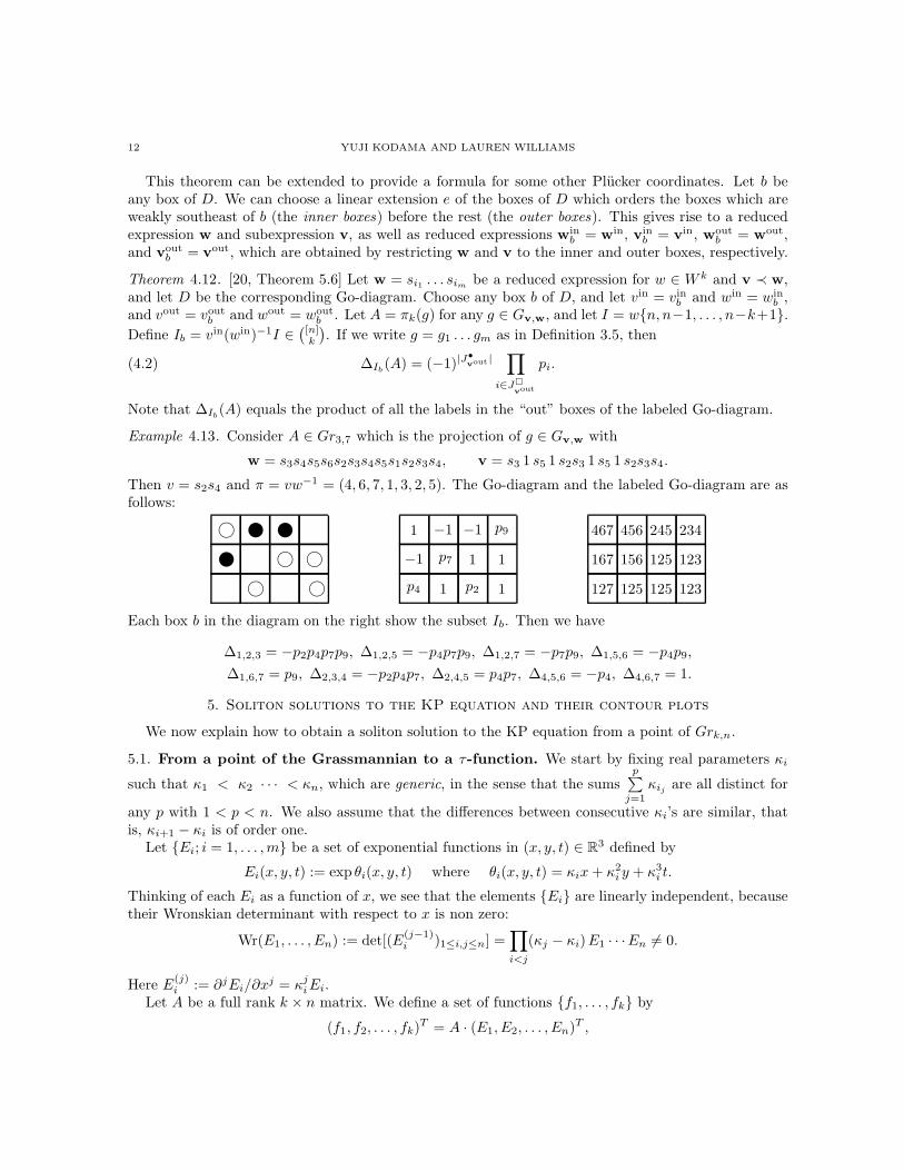
Example 4.13. Consider A ∈ Gr3,7 which is the projection of g ∈ Gv,w with
w = s3s4s5s6s2s3s4s5s1s2s3s4, v = s3 1 s5 1 s2s3 1 s5 1 s2s3s4.
Then v = s2s4 and π = vw−1 = (4, 6, 7, 1, 3, 2, 5). The Go-diagram and the labeled Go-diagram are asfollows:
② ②
②
1 −1 −1 p9
−1 p7 1 1
p4 1 p2 1
467 456 245 234
167 156 125 123
127 125 125 123
Each box b in the diagram on the right show the subset Ib. Then we have
∆1,2,3 = −p2p4p7p9, ∆1,2,5 = −p4p7p9, ∆1,2,7 = −p7p9, ∆1,5,6 = −p4p9,
∆1,6,7 = p9, ∆2,3,4 = −p2p4p7, ∆2,4,5 = p4p7, ∆4,5,6 = −p4, ∆4,6,7 = 1.
5. Soliton solutions to the KP equation and their contour plots
We now explain how to obtain a soliton solution to the KP equation from a point of Grk,n.
5.1. From a point of the Grassmannian to a τ-function. We start by fixing real parameters κi
such that κ1 < κ2 · · · < κn, which are generic, in the sense that the sumsp∑
j=1
κijare all distinct for
any p with 1 < p < n. We also assume that the differences between consecutive κi’s are similar, thatis, κi+1 − κi is of order one.
Let Ei; i = 1, . . . , m be a set of exponential functions in (x, y, t) ∈ R3 defined by
Ei(x, y, t) := exp θi(x, y, t) where θi(x, y, t) = κix + κ2i y + κ3
i t.
Thinking of each Ei as a function of x, we see that the elements Ei are linearly independent, becausetheir Wronskian determinant with respect to x is non zero:
Wr(E1, . . . , En) := det[(E(j−1)i )1≤i,j≤n] =
∏
i<j
(κj − κi)E1 · · ·En 6= 0.
Here E(j)i := ∂jEi/∂xj = κj
iEi.Let A be a full rank k × n matrix. We define a set of functions f1, . . . , fk by
(f1, f2, . . . , fk)T = A · (E1, E2, . . . , En)T ,
COMBINATORICS OF KP SOLITONS FROM THE REAL GRASSMANNIAN 13
where (. . .)T denotes the transpose of the vector (. . .).Since the exponential functions Ei are linearly independent, we identify them as a basis of Rn, and
then f1, . . . , fk spans a k-dimensional subspace. This identification can be seen, more precisely, asEi ↔ (1, κi, . . . , κ
n−1i )T ∈ Rn. This subspace depends only on which point of the Grassmannian Grk,n
the matrix A represents, so we can identify the space of subspaces f1, . . . , fk with Grk,n.The τ-function of A is defined by
(5.1) τA(x, y, t) := Wr(f1, f2, . . . , fk).
For I = i1, . . . , ik ∈(
[n]k
)
, we set
EI(x, y, t) := Wr(Ei1 , Ei2 , . . . , Eik) =
∏
ℓ<m
(κim− κiℓ
)Ei1 · · ·Eik> 0.
Applying the Binet-Cauchy identity to the fact that fj =n∑
i=1
ajiEi, we get
(5.2) τA(x, y, t) =∑
I∈([n]k )
∆I(A)EI(x, y, t).
It follows that if A ∈ (Grk,n)≥0, then τA > 0 for all (x, y, t) ∈ R3.Thinking of τA as a function of A, we note from (5.2) that the τ -function encodes the information
of the Plucker embedding. More specifically, if we identify each function EI with I = i1, . . . , ik withthe wedge product Ei1 ∧ · · · ∧ Eik
(recall the identification Ei ↔ (1, κi, . . . , κn−1i )T ), then the map
τ : Grk,n → RP(n
k)−1, A 7→ τA has the Plucker coordinates as coefficients.
5.2. From the τ-function to solutions of the KP equation. The KP equation for u(x, y, t)
∂
∂x
(
−4∂u
∂t+ 6u
∂u
∂x+
∂3u
∂x3
)
+ 3∂2u
∂y2= 0
was proposed by Kadomtsev and Petviashvili in 1970 [13], in order to study the stability of the solitonsolutions of the Korteweg-de Vries (KdV) equation under the influence of weak transverse perturbations.The KP equation can be also used to describe two-dimensional shallow water wave phenomena (see forexample [17]). This equation is now considered to be a prototype of an integrable nonlinear partialdifferential equation. For more background, see [24, 9, 1, 12, 23].
It is well known (see [12, 5, 6, 7]) that the τ -function defined in (5.1) provides a soliton solution ofthe KP equation,
(5.3) uA(x, y, t) = 2∂2
∂x2ln τA(x, y, t).
It is easy to show that if A ∈ (Grk,n)≥0, then such a solution uA(x, y, t) is regular for all (x, y, t) ∈ R3.For this reason we are interested in solutions uA(x, y, t) of the KP equation which come from points Aof (Grk,n)≥0. Throughout this paper when we speak of a soliton solution to the KP equation, we willmean a solution uA(x, y, t) which has form (5.3).
5.3. Contour plots of soliton solutions. One can visualize a solution uA(x, y, t) to the KP equationby drawing level sets of the solution in the xy-plane, when the coordinate t is fixed. For each r ∈ R,we denote the corresponding level set by
Cr(t) := (x, y) ∈ R2 : uA(x, y, t) = r.
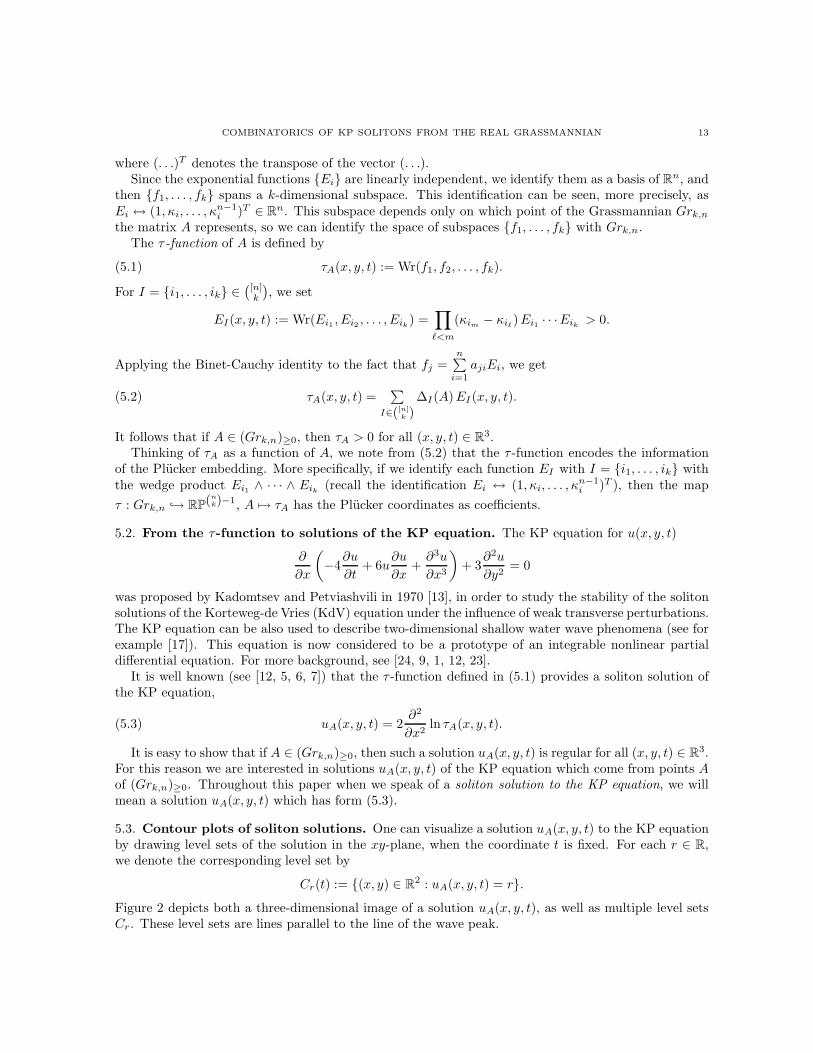
Figure 2 depicts both a three-dimensional image of a solution uA(x, y, t), as well as multiple level setsCr. These level sets are lines parallel to the line of the wave peak.
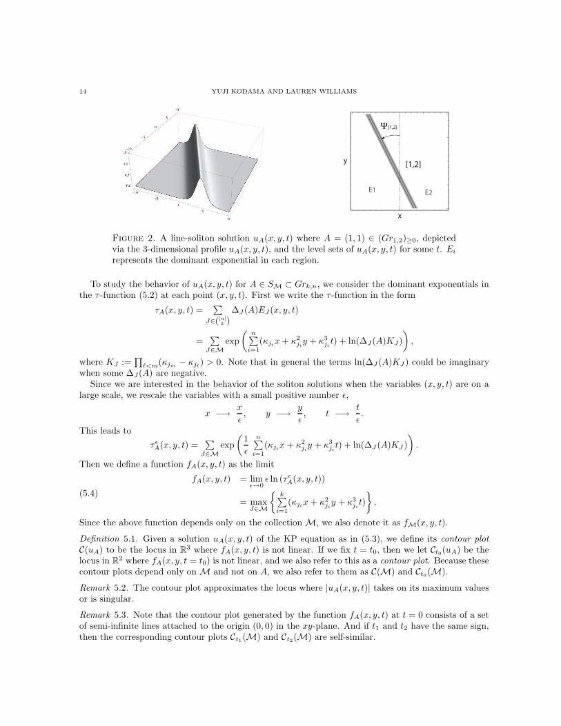
14 YUJI KODAMA AND LAUREN WILLIAMS
[1,2]
Ψ[1,2]
x
y
E1 E2
Figure 2. A line-soliton solution uA(x, y, t) where A = (1, 1) ∈ (Gr1,2)≥0, depictedvia the 3-dimensional profile uA(x, y, t), and the level sets of uA(x, y, t) for some t. Ei
represents the dominant exponential in each region.
To study the behavior of uA(x, y, t) for A ∈ SM ⊂ Grk,n, we consider the dominant exponentials inthe τ -function (5.2) at each point (x, y, t). First we write the τ -function in the form
τA(x, y, t) =∑
J∈([n]k )
∆J (A)EJ (x, y, t)
=∑
J∈M
exp
(
n∑
i=1
(κjix + κ2
jiy + κ3
jit) + ln(∆J (A)KJ)
)
,
where KJ :=∏
ℓ<m(κjm− κjℓ
) > 0. Note that in general the terms ln(∆J (A)KJ ) could be imaginarywhen some ∆J(A) are negative.
Since we are interested in the behavior of the soliton solutions when the variables (x, y, t) are on alarge scale, we rescale the variables with a small positive number ǫ,
x −→x
ǫ, y −→
y
ǫ, t −→
t
ǫ.
This leads to
τ ǫA(x, y, t) =
∑
J∈M
exp
(
1
ǫ
n∑
i=1
(κjix + κ2
jiy + κ3
jit) + ln(∆J (A)KJ )
)
.
Then we define a function fA(x, y, t) as the limit
(5.4)
fA(x, y, t) = limǫ→0
ǫ ln (τ ǫA(x, y, t))
= maxJ∈M
k∑
i=1
(κjix + κ2
jiy + κ3
jit)
.
Since the above function depends only on the collectionM, we also denote it as fM(x, y, t).
Definition 5.1. Given a solution uA(x, y, t) of the KP equation as in (5.3), we define its contour plotC(uA) to be the locus in R3 where fA(x, y, t) is not linear. If we fix t = t0, then we let Ct0(uA) be thelocus in R2 where fA(x, y, t = t0) is not linear, and we also refer to this as a contour plot. Because thesecontour plots depend only onM and not on A, we also refer to them as C(M) and Ct0(M).
Remark 5.2. The contour plot approximates the locus where |uA(x, y, t)| takes on its maximum valuesor is singular.
Remark 5.3. Note that the contour plot generated by the function fA(x, y, t) at t = 0 consists of a setof semi-infinite lines attached to the origin (0, 0) in the xy-plane. And if t1 and t2 have the same sign,then the corresponding contour plots Ct1(M) and Ct2(M) are self-similar.
COMBINATORICS OF KP SOLITONS FROM THE REAL GRASSMANNIAN 15
Also note that because our definition of the contour plot ignores the constant terms ln(∆J (A)KJ ),there are no phase-shifts in our picture, and the contour plot for fA(x, y, t) = fM(x, y, t) does notdepend on the signs of the Plucker coordinates.
It follows from Definition 5.1 that C(uA) and Ct0(uA) are piecewise linear subsets of R3 and R2,respectively, of codimension 1. In fact it is easy to verify the following.
Proposition 5.4. [19, Proposition 4.3] If each κi is an integer, then C(uA) is a tropical hypersurface inR3, and Ct0(uA) is a tropical hypersurface (i.e. a tropical curve) in R2.
The contour plot Ct0(uA) consists of line segments called line-solitons, some of which have finitelength, while others are unbounded and extend in the y direction to ±∞. Each region of the complementof Ct0(uA) in R2 is a domain of linearity for fA(x, y, t), and hence each region is naturally associated toa dominant exponential ∆J (A)EJ (x, y, t) from the τ -function (5.2). We label this region by J or EJ .Each line-soliton represents a balance between two dominant exponentials in the τ -function.
Because of the genericity of the κ-parameters, the following lemma is immediate.
Lemma 5.5. [7, Proposition 5] The index sets of the dominant exponentials of the τ -function in adjacentregions of the contour plot in the xy-plane are of the form i, l2, . . . , lk and j, l2, . . . , lk.
We call the line-soliton separating the two dominant exponentials in Lemma 5.5 a line-soliton of type[i, j]. Its equation is
(5.5) x + (κi + κj)y + (κ2i + κiκj + κ2
j)t = 0.
Remark 5.6. Consider a line-soliton given by (5.5). Compute the angle Ψ[i,j] between the positive y-axisand the line-soliton of type [i, j], measured in the counterclockwise direction, so that the negative x-axishas an angle of π
2 and the positive x-axis has an angle of −π2 . Then tan Ψ[i,j] = κi + κj , so we refer to
κi + κj as the slope of the [i, j] line-soliton (see Figure 2).
In Section 7 we will explore the combinatorial structure of contour plots, that is, the ways in whichline-solitons may interact. Generically we expect a point at which several line-solitons meet to havedegree 3; we regard such a point as a trivalent vertex. Three line-solitons meeting at a trivalent vertexexhibit a resonant interaction (this corresponds to the balancing condition for a tropical curve). See[19, Section 4.2]. One may also have two line-solitons which cross over each other, forming an X-shape:we call this an X-crossing, but do not regard it as a vertex. See Figure 4. Vertices of degree greaterthan 4 are also possible.
Definition 5.7. Let i < j < k < ℓ be positive integers. An X-crossing involving two line-solitons oftypes [i, k] and [j, ℓ] is called a black X-crossing. An X-crossing involving two line-solitons of types [i, j]and [k, ℓ], or of types [i, ℓ] and [j, k], is called a white X-crossing.
Definition 5.8. A contour plot Ct(uA) is called generic if all interactions of line-solitons are at trivalentvertices or are X-crossings.
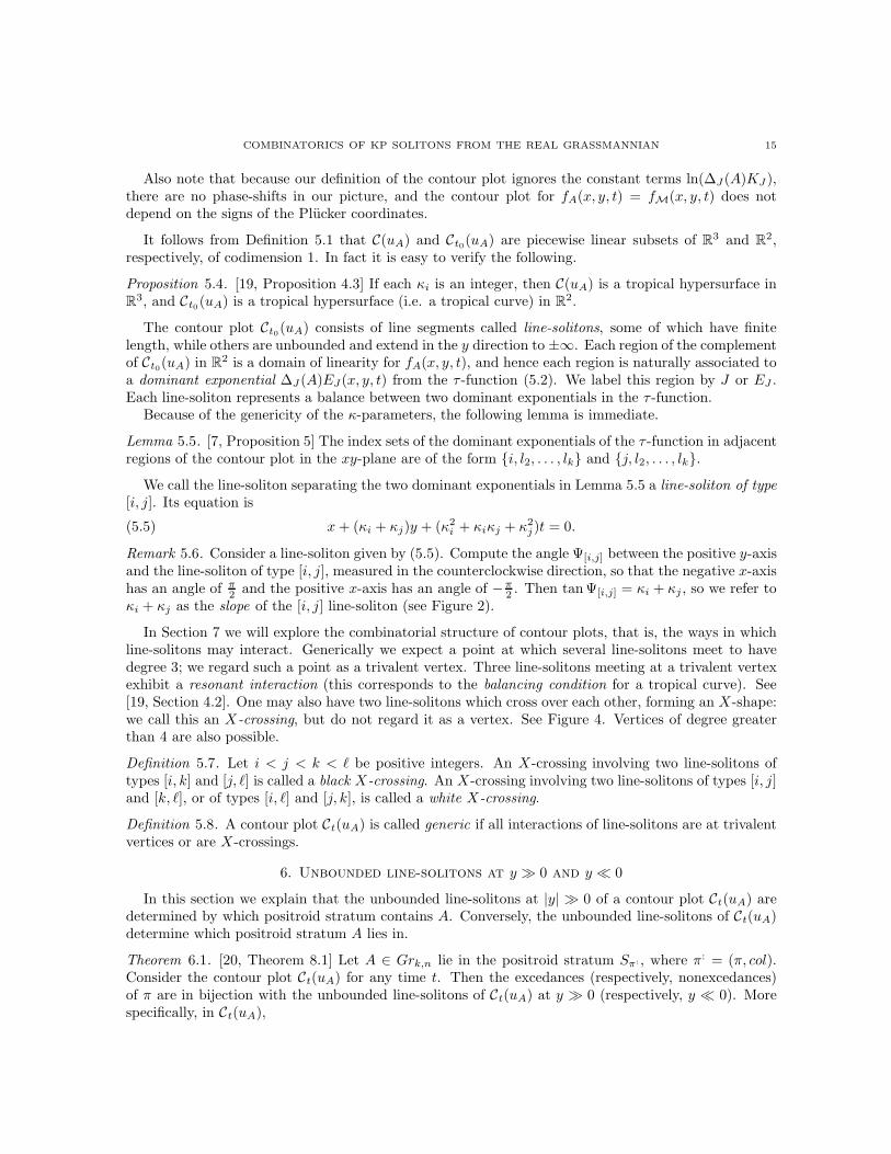
6. Unbounded line-solitons at y ≫ 0 and y ≪ 0
In this section we explain that the unbounded line-solitons at |y| ≫ 0 of a contour plot Ct(uA) aredetermined by which positroid stratum contains A. Conversely, the unbounded line-solitons of Ct(uA)determine which positroid stratum A lies in.
Theorem 6.1. [20, Theorem 8.1] Let A ∈ Grk,n lie in the positroid stratum Sπ: , where π: = (π, col).Consider the contour plot Ct(uA) for any time t. Then the excedances (respectively, nonexcedances)of π are in bijection with the unbounded line-solitons of Ct(uA) at y ≫ 0 (respectively, y ≪ 0). Morespecifically, in Ct(uA),
16 YUJI KODAMA AND LAUREN WILLIAMS
(a) there is an unbounded line-soliton of [i, h]-type at y ≫ 0 if and only if π(i) = h for i < h,(b) there is an unbounded line-soliton of [i, h]-type at y ≪ 0 if and only if π(h) = i for i < h.
Therefore π: determines the unbounded line-solitons at y ≫ 0 and y ≪ 0 of Ct(uA) for any time t.Conversely, given a contour plot Ct(uA) at any time t where A ∈ Grk,n, one can construct π: = (π, col)
such that A ∈ Sπ: as follows. The excedances and nonexcedances of π are constructed as above fromthe unbounded line-solitons. If there is an h ∈ [n] such that h ∈ J for every dominant exponential EJ
labeling the contour plot, then set π(h) = h with col(h) = 1. If there is an h ∈ [n] such that h /∈ J forany dominant exponential EJ labeling the contour plot, then set π(h) = h with col(h) = −1.
Remark 6.2. Chakravarty and Kodama [5, Prop. 2.6 and 2.9] and [7, Theorem 5] associated a derange-ment to each irreducible element A in the totally non-negative part (Grk,n)≥0 of the Grassmannian.Theorem 6.1 generalizes their result by dropping the hypothesis of irreducibility and extending thesetting from (Grk,n)≥0 to Grk,n.
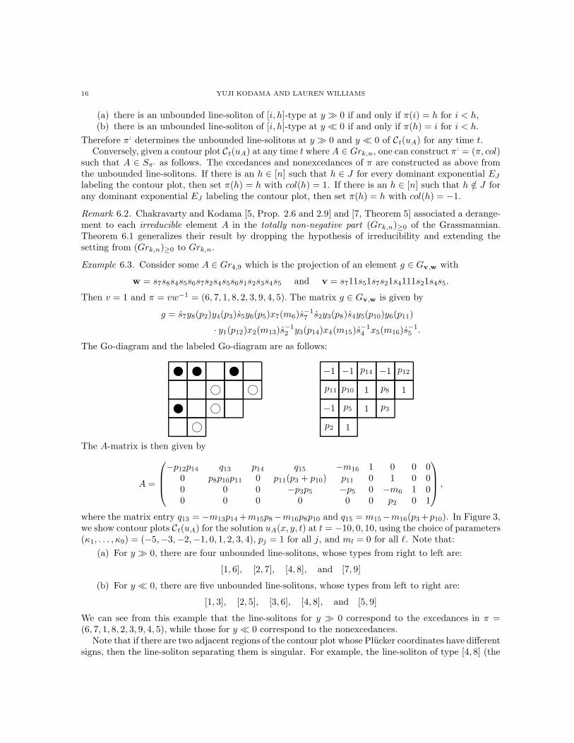
Example 6.3. Consider some A ∈ Gr4,9 which is the projection of an element g ∈ Gv,w with
w = s7s8s4s5s6s7s2s4s5s6s1s2s3s4s5 and v = s711s51s7s21s4111s21s4s5.
Then v = 1 and π = vw−1 = (6, 7, 1, 8, 2, 3, 9, 4, 5). The matrix g ∈ Gv,w is given by
g = s7y8(p2)y4(p3)s5y6(p5)x7(m6)s−17 s2y3(p8)s4y5(p10)y6(p11)
· y1(p12)x2(m13)s−12 y3(p14)x4(m15)s
−14 x5(m16)s
−15 .
The Go-diagram and the labeled Go-diagram are as follows:
② ② ②
②
−1 −1 p14 −1 p12
p11 p10 1 p8 1
−1 p5 1 p3
p2 1
The A-matrix is then given by
A =
−p12p14 q13 p14 q15 −m16 1 0 0 00 p8p10p11 0 p11(p3 + p10) p11 0 1 0 00 0 0 −p3p5 −p5 0 −m6 1 00 0 0 0 0 0 p2 0 1
,
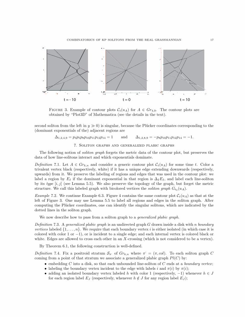
where the matrix entry q13 = −m13p14 +m15p8−m16p8p10 and q15 = m15−m16(p3 +p10). In Figure 3,we show contour plots Ct(uA) for the solution uA(x, y, t) at t = −10, 0, 10, using the choice of parameters(κ1, . . . , κ9) = (−5,−3,−2,−1, 0, 1, 2, 3, 4), pj = 1 for all j, and ml = 0 for all ℓ. Note that:
(a) For y ≫ 0, there are four unbounded line-solitons, whose types from right to left are:
[1, 6], [2, 7], [4, 8], and [7, 9]
(b) For y ≪ 0, there are five unbounded line-solitons, whose types from left to right are:
[1, 3], [2, 5], [3, 6], [4, 8], and [5, 9]
We can see from this example that the line-solitons for y ≫ 0 correspond to the excedances in π =(6, 7, 1, 8, 2, 3, 9, 4, 5), while those for y ≪ 0 correspond to the nonexcedances.
Note that if there are two adjacent regions of the contour plot whose Plucker coordinates have differentsigns, then the line-soliton separating them is singular. For example, the line-soliton of type [4, 8] (the
COMBINATORICS OF KP SOLITONS FROM THE REAL GRASSMANNIAN 17
t = - 10 t = 0 t = 10
Figure 3. Example of contour plots Ct(uA) for A ∈ Gr4,9. The contour plots areobtained by “Plot3D” of Mathematica (see the details in the text).
second soliton from the left in y ≫ 0) is singular, because the Plucker coordinates corresponding to the(dominant exponentials of the) adjacent regions are
∆1,2,4,9 = p3p5p8p10p11p12p14 = 1 and ∆1,2,8,9 = −p8p10p11p12p14 = −1.
7. Soliton graphs and generalized plabic graphs
The following notion of soliton graph forgets the metric data of the contour plot, but preserves thedata of how line-solitons interact and which exponentials dominate.
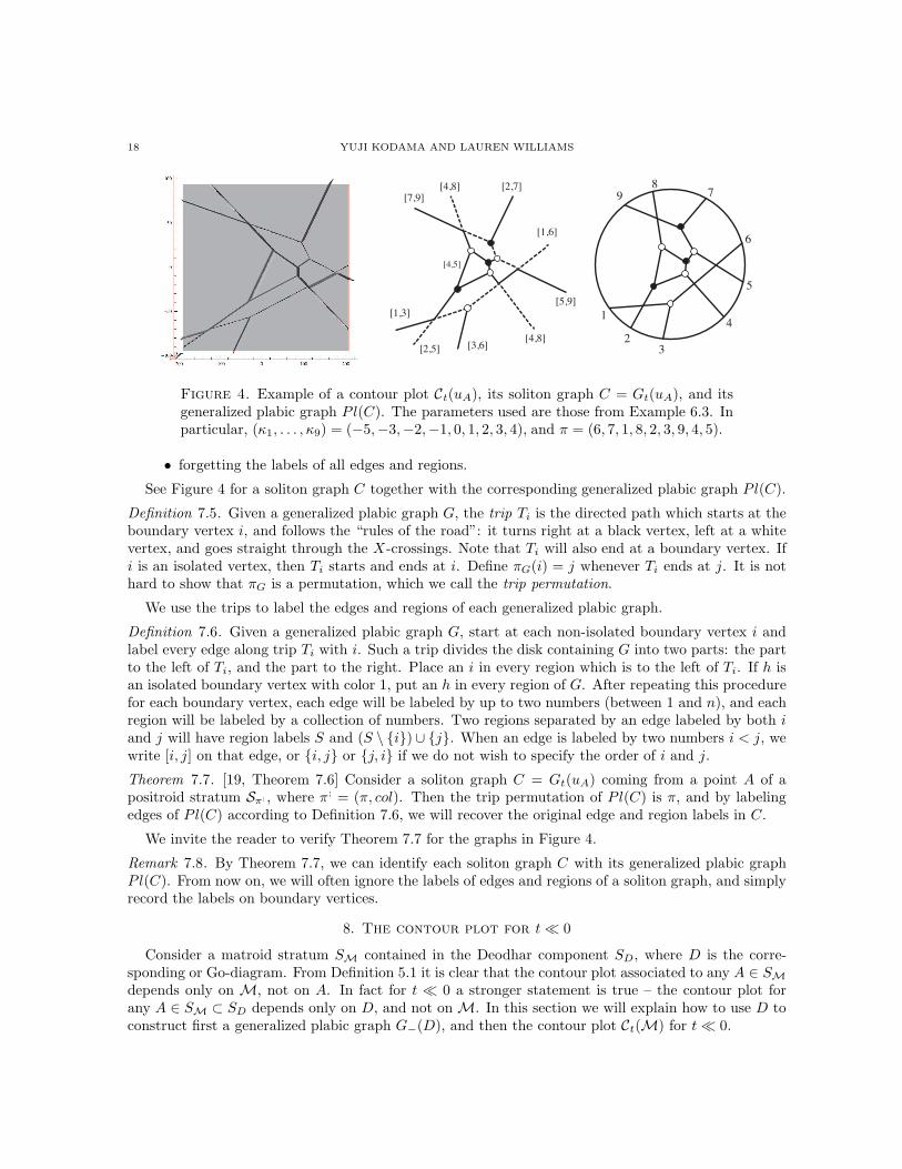
Definition 7.1. Let A ∈ Grk,n and consider a generic contour plot Ct(uA) for some time t. Color atrivalent vertex black (respectively, white) if it has a unique edge extending downwards (respectively,upwards) from it. We preserve the labeling of regions and edges that was used in the contour plot: welabel a region by EI if the dominant exponential in that region is ∆IEI , and label each line-solitonby its type [i, j] (see Lemma 5.5). We also preserve the topology of the graph, but forget the metricstructure. We call this labeled graph with bicolored vertices the soliton graph Gt0(uA).
Example 7.2. We continue Example 6.3. Figure 4 contains the same contour plot Ct(uA) as that at theleft of Figure 3. One may use Lemma 5.5 to label all regions and edges in the soliton graph. Aftercomputing the Plucker coordinates, one can identify the singular solitons, which are indicated by thedotted lines in the soliton graph.
We now describe how to pass from a soliton graph to a generalized plabic graph.
Definition 7.3. A generalized plabic graph is an undirected graph G drawn inside a disk with n boundaryvertices labeled 1, . . . , n. We require that each boundary vertex i is either isolated (in which case it iscolored with color 1 or −1), or is incident to a single edge; and each internal vertex is colored black orwhite. Edges are allowed to cross each other in an X-crossing (which is not considered to be a vertex).
By Theorem 6.1, the following construction is well-defined.
Definition 7.4. Fix a positroid stratum Sπ: of Grk,n where π: = (π, col). To each soliton graph Ccoming from a point of that stratum we associate a generalized plabic graph Pl(C) by:
• embedding C into a disk, so that each unbounded line-soliton of C ends at a boundary vertex ;• labeling the boundary vertex incident to the edge with labels i and π(i) by π(i);• adding an isolated boundary vertex labeled h with color 1 (respectively, −1) whenever h ∈ J
for each region label EJ (respectively, whenever h /∈ J for any region label EJ );
18 YUJI KODAMA AND LAUREN WILLIAMS
[4,8][7,9]
[2,7]
[1,6]
[5,9]
[4,8][3,6]
[1,3]
[2,5]
[4,5]
1
23
4
5
6
78
9
Figure 4. Example of a contour plot Ct(uA), its soliton graph C = Gt(uA), and itsgeneralized plabic graph Pl(C). The parameters used are those from Example 6.3. Inparticular, (κ1, . . . , κ9) = (−5,−3,−2,−1, 0, 1, 2, 3, 4), and π = (6, 7, 1, 8, 2, 3, 9, 4, 5).
• forgetting the labels of all edges and regions.
See Figure 4 for a soliton graph C together with the corresponding generalized plabic graph Pl(C).
Definition 7.5. Given a generalized plabic graph G, the trip Ti is the directed path which starts at theboundary vertex i, and follows the “rules of the road”: it turns right at a black vertex, left at a whitevertex, and goes straight through the X-crossings. Note that Ti will also end at a boundary vertex. Ifi is an isolated vertex, then Ti starts and ends at i. Define πG(i) = j whenever Ti ends at j. It is nothard to show that πG is a permutation, which we call the trip permutation.
We use the trips to label the edges and regions of each generalized plabic graph.
Definition 7.6. Given a generalized plabic graph G, start at each non-isolated boundary vertex i andlabel every edge along trip Ti with i. Such a trip divides the disk containing G into two parts: the partto the left of Ti, and the part to the right. Place an i in every region which is to the left of Ti. If h isan isolated boundary vertex with color 1, put an h in every region of G. After repeating this procedurefor each boundary vertex, each edge will be labeled by up to two numbers (between 1 and n), and eachregion will be labeled by a collection of numbers. Two regions separated by an edge labeled by both iand j will have region labels S and (S \ i)∪ j. When an edge is labeled by two numbers i < j, wewrite [i, j] on that edge, or i, j or j, i if we do not wish to specify the order of i and j.
Theorem 7.7. [19, Theorem 7.6] Consider a soliton graph C = Gt(uA) coming from a point A of apositroid stratum Sπ: , where π: = (π, col). Then the trip permutation of Pl(C) is π, and by labelingedges of Pl(C) according to Definition 7.6, we will recover the original edge and region labels in C.
We invite the reader to verify Theorem 7.7 for the graphs in Figure 4.
Remark 7.8. By Theorem 7.7, we can identify each soliton graph C with its generalized plabic graphPl(C). From now on, we will often ignore the labels of edges and regions of a soliton graph, and simplyrecord the labels on boundary vertices.
8. The contour plot for t≪ 0
Consider a matroid stratum SM contained in the Deodhar component SD, where D is the corre-sponding or Go-diagram. From Definition 5.1 it is clear that the contour plot associated to any A ∈ SM
depends only on M, not on A. In fact for t ≪ 0 a stronger statement is true – the contour plot forany A ∈ SM ⊂ SD depends only on D, and not onM. In this section we will explain how to use D toconstruct first a generalized plabic graph G−(D), and then the contour plot Ct(M) for t≪ 0.
COMBINATORICS OF KP SOLITONS FROM THE REAL GRASSMANNIAN 19
8.1. Definition of the contour plot for t ≪ 0. Recall from (5.4) the definition of fM(x, y, t). Tounderstand how it behaves for t≪ 0, let us rescale everything by t. Define x = x
tand y = y
t, and set
φi(x, y) = κix + κ2i y + κ3
i ,
that is, κix + κ2i y + κ3
i t = tφi(x, y). Note that because t is negative, x and y have the opposite signs ofx and y. This leads to the following definition of the contour plot for t≪ 0.
Definition 8.1. We define the contour plot C−∞(M) to be the locus in R2 where
minJ∈M
k∑
i=1
φji(x, y)
is not linear .
Remark 8.2. After a 180 rotation, C−∞(M) is the limit of Ct(uA) as t → −∞, for any A ∈ SM.Note that the rotation is required because the positive x-axis (respectively, y-axis) corresponds to thenegative x-axis (respectively, y-axis).
Definition 8.3. Define vi,ℓ,m to be the point in R2 where φi(x, y) = φℓ(x, y) = φm(x, y). A simplecalculation yields that the point vi,ℓ,m has the following coordinates in the xy-plane:
vi,ℓ,m = (κiκℓ + κiκm + κℓκm,−(κi + κℓ + κm)).
Some of the points vi,ℓ,m ∈ R2 correspond to trivalent vertices in the contour plots we construct;such a point is the location of the resonant interaction of three line-solitons of types [i, ℓ], [ℓ, m] and[i, m] (see Theorem 8.5 below). Because of our assumption on the genericity of the κ-parameters, thosepoints are all distinct.
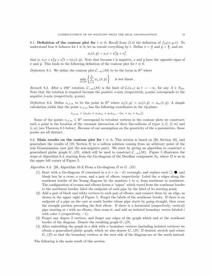
8.2. Main results on the contour plot for t ≪ 0. This section is based on [20, Section 10], andgeneralizes the results of [19, Section 8] to a soliton solution coming from an arbitrary point of thereal Grassmannian (not just the non-negative part). We start by giving an algorithm to construct ageneralized plabic graph G−(D), which will be used to construct C−∞(M). Figure 5 illustrates thesteps of Algorithm 8.4, starting from the Go-diagram of the Deodhar component SD where D is as inthe upper left corner of Figure 5.
Algorithm 8.4. [20, Algorithm 10.4] From a Go-diagram D to G−(D):
(1) Start with a Go-diagram D contained in a k × (n − k) rectangle, and replace each , , andblank box by a cross, a cross, and a pair of elbows, respectively. Label the n edges along thesoutheast border of the Young diagram by the numbers 1 to n, from northeast to southwest.The configuration of crosses and elbows forms n “pipes” which travel from the southeast borderto the northwest border; label the endpoint of each pipe by the label of its starting point.
(2) Add a pair of black and white vertices to each pair of elbows, and connect them by an edge, asshown in the upper right of Figure 5. Forget the labels of the southeast border. If there is anendpoint of a pipe on the east or south border whose pipe starts by going straight, then erasethe straight portion preceding the first elbow. If there is a horizontal (respectively, vertical)pipe starting at i with no elbows, then erase it, and add an isolated boundary vertex labeled iwith color 1 (respectively, −1).
(3) Forget any degree 2 vertices, and forget any edges of the graph which end at the southeastborder of the diagram. Denote the resulting graph G−(D).
(4) After embedding the graph in a disk with n boundary vertices (including isolated vertices) weobtain a generalized plabic graph, which we also denote G−(D). If desired, stretch and rotateG−(D) so that the boundary vertices at the west side of the diagram are at the north instead.
The following is the main result of this section.
20 YUJI KODAMA AND LAUREN WILLIAMS
1
2
34
5
8 7 6
5
7
5
6
8
2 4 3 1 2 4 3 1
5
7
5
6
8
5
7
5
6
8
1
2 34
(1245)
(5678)
(1268)(1258)
(1678)
1
3
4
2
5
76
8
(1245)
(1268)
(1678)
(2345)
(2345)
Figure 5. Construction of the generalized plabic graph G−(D) associated to the Go-diagram D. The labels of the regions of the graph indicate the index sets of thecorresponding Plucker coordinates. Using the notation of Definition 4.7, we haveπ(D) = vw−1 = (5, 7, 1, 6, 8, 3, 4, 2).
Theorem 8.5. [20, Theorem 10.6] Choose a matroid stratum SM and let SD be the Deodhar componentcontaining SM. Recall the definition of π(D) from Definition 4.7. Use Algorithm 8.4 to obtain G−(D).Then G−(D) has trip permutation π(D), and we can use it to explicitly construct C−∞(M) as follows.Label the edges of G−(D) according to the rules of the road. Label by vi,ℓ,m each trivalent vertexwhich is incident to edges labeled [i, ℓ], [i, m], and [ℓ, m], and give that vertex the coordinates (x, y) =(κiκℓ + κiκm + κℓκm,−(κi + κℓ + κm)). Replace each edge labeled [i, j] which ends at a boundaryvertex by an unbounded line-soliton with slope κi + κj . (Each edge labeled [i, j] between two trivalentvertices will automatically have slope κi +κj.) In particular, C−∞(M) is determined by D. Recall fromRemark 8.2 that after a 180 rotation, C−∞(M) is the limit of Ct(uA) as t→ −∞, for any A ∈ SM.
Remark 8.6. Since the contour plot C−∞(M) depends only on D, we also refer to it as C−∞(D).
Remark 8.7. The results of this section may be extended to the case t ≫ 0 by duality considerations(similar to the way in which our previous paper [19] described contour plots for both t≪ 0 and t≫ 0).Note that the Deodhar decomposition of Grk,n depends on a choice of ordered basis (e1, . . . , en). Usingthe ordered basis (en, . . . , e1) instead and the corresponding Deodhar decomposition, one may explicitlydescribe contour plots at t≫ 0.
Remark 8.8. Depending on the choice of the parameters κi, the contour plot C−∞(D) may have aslightly different topological structure than the soliton graph G−(D). While the incidences of line-solitons with trivalent vertices are determined by G−(D), the locations of X-crossings may vary basedon the κi’s. More specifically, changing the κi’s may change the contour plot via a sequence of slides,see [20, Section 11].
COMBINATORICS OF KP SOLITONS FROM THE REAL GRASSMANNIAN 21
8.3. X-crossings in the contour plots. Recall the notions of black and white X-crossings fromDefinition 5.7. In [19, Theorem 9.1], we proved that the presence of X-crossings in contour plots at|t| ≫ 0 implies that there is a two-term Plucker relation.
Theorem 8.9. [19, Theorem 9.1] Suppose that there is an X-crossing in a contour plot Ct(uA) for someA ∈ Grk,n where |t| ≫ 0. Let I1, I2, I3, and I4 be the k-element subsets of 1, . . . , n corresponding tothe dominant exponentials incident to the X-crossing listed in circular order.
• If the X-crossing is white, we have ∆I1(A)∆I3 (A) = ∆I2 (A)∆I4 (A).• If the X-crossing is black, we have ∆I1 (A)∆I3 (A) = −∆I2(A)∆I4 (A).
The following corollary is immediate.
Corollary 8.10. If there is a black X-crossing in a contour plot at t ≪ 0 or t ≫ 0, then among thePlucker coordinates associated to the dominant exponentials incident to that black X-crossing, threemust be positive and one negative, or vice-versa.
Corollary 8.11. Let D be a
Γ
-diagram, that is, a Go-diagram with no black stones. Let A ∈ SD andt≪ 0. Choose any κ1 < · · · < κn. Then the contour plot Ct(uA) can have only white X-crossings.
9. Total positivity, regularity, and cluster algebras
In this paper we have been studying solutions uA(x, y, t) to the KP equation coming from points of thereal Grassmannian. Among these solutions, those coming from the totally non-negative part of Grk,n
are especially nice. In particular, (Grk,n)≥0 parameterizes the regular soliton solutions coming fromGrk,n, see Theorem 9.1. This result provides an important motivation for studying the soliton solutionscoming from (Grk,n)≥0. After discussing the regularity result below, we will discuss positivity tests forelements of the Grassmannian, as well as the connection between soliton solutions from (Grk,n)>0 andthe theory of cluster algebras.
Theorem 9.1. [20, Theorem 12.1] Fix parameters κ1 < · · · < κn and an element A ∈ Grk,n. Considerthe corresponding soliton solution uA(x, y, t) of the KP equation. This solution is regular at t ≪ 0 ifand only if A ∈ (Grk,n)≥0. Therefore this solution is regular for all times t if and only if A ∈ (Grk,n)≥0.
If one is studying total positivity on the Grassmannian, then a natural question is the following: givenA ∈ Grk,n, how many Plucker coordinates, and which ones, must one compute, in order to determinethat A ∈ (Grk,n)≥0? This leads to the following notion of positivity test.
Definition 9.2. Consider the Deodhar component SD ⊂ Grk,n, where D is a Go-diagram. A collectionJ of k-element subsets of 1, 2, . . . , n is called a positivity test for SD if for any A ∈ SD, the conditionthat ∆I(A) > 0 for all I ∈ J implies that A ∈ (Grk,n)≥0.
It turns out that the collection of Plucker coordinates corresponding to dominant exponentials incontour plots at t≪ 0 provide positivity tests for positroid strata.
Theorem 9.3. [20, Theorem 12.9] Let A ∈ SD ⊂ Grk,n, where D is a
Γ
-diagram, and let t ≪ 0. If∆J (A) > 0 for each dominant exponential EJ in the contour plot Ct(uA), then A ∈ (Grk,n)≥0. Inother words, the Plucker coordinates corresponding to the dominant exponentials in Ct(uA) comprise apositivity test for SD.
Remark 9.4. Recall that the Deodhar components SD have non-empty intersection with (Grk,n)≥0
unless D is a
Γ
-diagram. Therefore Theorem 9.3 restricts to the case that D is a
Γ
-diagram.
22 YUJI KODAMA AND LAUREN WILLIAMS
9.1. TP Schubert cells and reduced plabic graphs. In this section we provide a new characteri-zation of the so-called reduced plabic graphs [25, Section 12]. This will allow us to make a connectionto cluster algebras in Section 9.2.
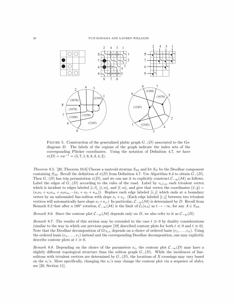
We will always assume that a plabic graph is leafless, i.e. that it has no non-boundary leaves, andthat it has no isolated components. In order to define reduced, we first define some local transformationsof plabic graphs.
(M1) SQUARE MOVE. If a plabic graph has a square formed by four trivalent vertices whose colorsalternate, then we can switch the colors of these four vertices.
(M2) UNICOLORED EDGE CONTRACTION/UNCONTRACTION. If a plabic graph contains anedge with two vertices of the same color, then we can contract this edge into a single vertex with thesame color. We can also uncontract a vertex into an edge with vertices of the same color.
(M3) MIDDLE VERTEX INSERTION/REMOVAL. If a plabic graph contains a vertex of degree 2,then we can remove this vertex and glue the incident edges together; on the other hand, we can alwaysinsert a vertex (of any color) in the middle of any edge.
Figure 6. A square move; a unicolored edge contraction; a middle vertex insertion/ removal
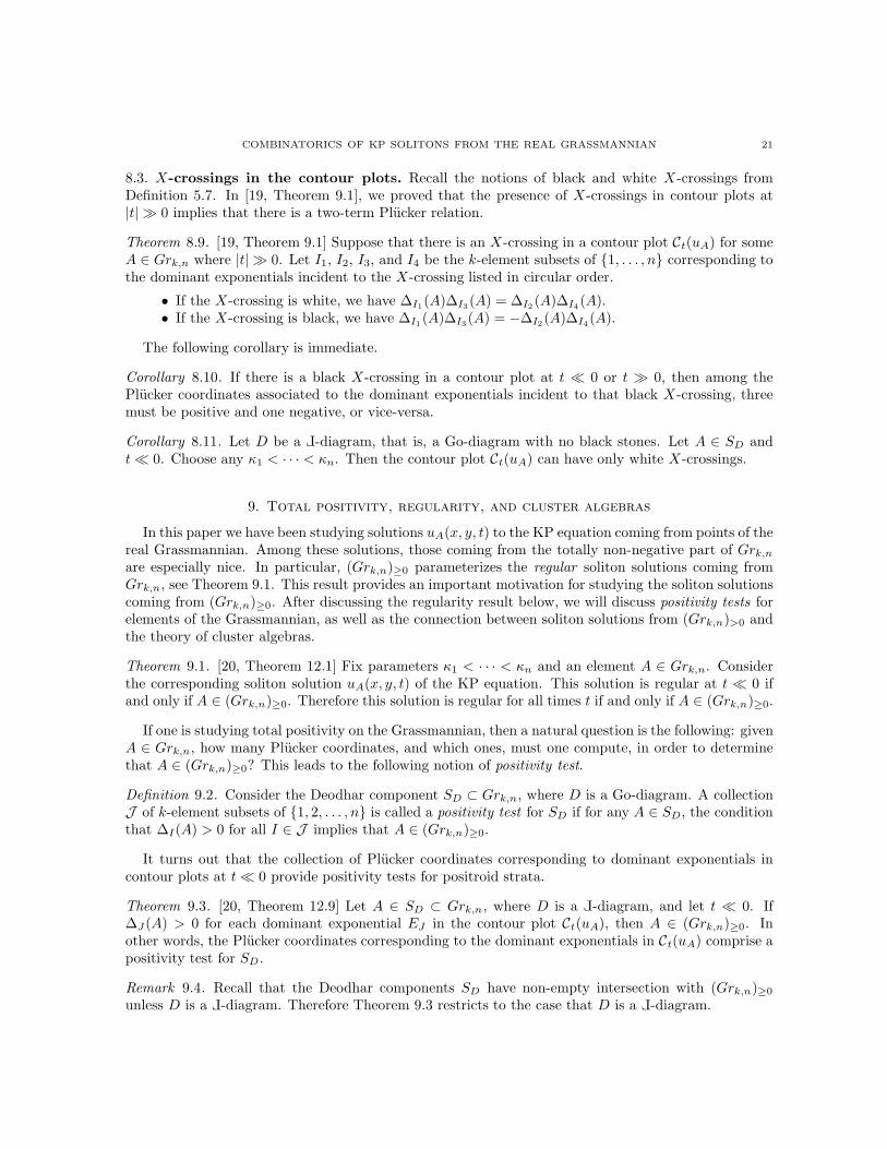
(R1) PARALLEL EDGE REDUCTION. If a network contains two trivalent vertices of differentcolors connected by a pair of parallel edges, then we can remove these vertices and edges, and glue theremaining pair of edges together.
Figure 7. Parallel edge reduction
Definition 9.5. [25] Two plabic graphs are called move-equivalent if they can be obtained from eachother by moves (M1)-(M3). The move-equivalence class of a given plabic graph G is the set of all plabicgraphs which are move-equivalent to G. A leafless plabic graph without isolated components is calledreduced if there is no graph in its move-equivalence class to which we can apply (R1).
Theorem 9.6. [25, Theorem 13.4] Two reduced plabic graphs which each have n boundary vertices aremove-equivalent if and only if they have the same trip permutation.
Our new characterization of reduced plabic graphs is as follows.
Definition 9.7. We say that a (generalized) plabic graph has the resonance property, if after labelingedges via Definition 7.6, the set E of edges incident to a given vertex has the following property:
• there exist numbers i1 < i2 < · · · < im such that when we read the labels of E, we see thelabels [i1, i2], [i2, i3], . . . , [im−1, im], [i1, im] appear in counterclockwise order.
Theorem 9.8. [19, Theorem 10.5]. A plabic graph is reduced if and only if it has the resonance property.6
Corollary 9.9. [19, Corollary 10.9] Suppose that A lies in a TP Schubert cell, and that for some timet, Gt(uA) is generic with no X-crossings. Then Gt(uA) is a reduced plabic graph.
6Recall from Definition 2.11 that our convention is to label boundary vertices of a plabic graph 1, 2, . . . , n in counter-clockwise order. If one chooses the opposite convention, then one must replace the word counterclockwise in Definition9.7 by clockwise.
COMBINATORICS OF KP SOLITONS FROM THE REAL GRASSMANNIAN 23
9.2. The connection to cluster algebras. Cluster algebras are a class of commutative rings, intro-duced by Fomin and Zelevinsky [10], which have a remarkable combinatorial structure. Many coordinaterings of homogeneous spaces have a cluster algebra structure: as shown by Scott [28], the Grassmannianis one such example.
Theorem 9.10. [28] The coordinate ring of (the affine cone over) Grk,n has a cluster algebra structure.Moreover, the set of Plucker coordinates whose indices come from the labels of the regions of a reducedplabic graph for (Grk,n)>0 comprises a cluster for this cluster algebra.
Remark 9.11. In fact [28] used the combinatorics of alternating strand diagrams, not reduced plabicgraphs, to describe clusters. However, alternating strand diagrams are in bijection with reduced plabicgraphs [25].
Theorem 9.12. [19, 10.12] The set of Plucker coordinates labeling regions of a generic trivalent solitongraph for the TP Grassmannian is a cluster for the cluster algebra associated to the Grassmannian.
Conjecturally, every positroid cell Stnnπ of the totally non-negative Grassmannian also carries a
cluster algebra structure, and the Plucker coordinates labeling the regions of any reduced plabic graphfor Stnn
π should be a cluster for that cluster algebra. In particular, the TP Schubert cells shouldcarry cluster algebra structures. Therefore we conjecture that Theorem 9.12 holds with “Schubertcell” replacing “Grassmannian.” Finally, there should be a suitable generalization of Theorem 9.12 forarbitrary positroid cells.
9.3. Soliton graphs for (Gr2,n)>0 and triangulations of an n-gon. In this section we must use aslightly more general setup for τ -functions τA(t1, . . . , tm) and soliton solutions uA(t1, . . . , tm), in whichthe exponential functions Ei and EI are functions of variables t1, . . . , tm, and m ≥ n. Here t1 = x,t2 = y, t3 = t, and the other ti’s are referred to as higher times. See [19, Section 3] for details.
1
2
3 4
5
6
[2,6] [1,5]
[3,5][2,4]
[4,6][1,3]
1
2
3 4
5
6
E16
E12
E23
E34
E45
E56E26
E25
E35
[2,6][1,5]
[3,5][2,4]
[4,6]
[1,3]
Soliton graph Contour plot
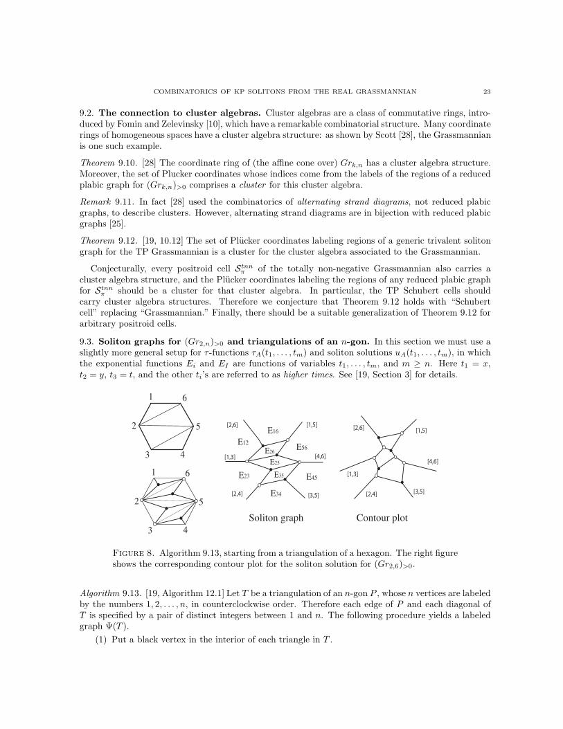
Figure 8. Algorithm 9.13, starting from a triangulation of a hexagon. The right figureshows the corresponding contour plot for the soliton solution for (Gr2,6)>0.
Algorithm 9.13. [19, Algorithm 12.1] Let T be a triangulation of an n-gon P , whose n vertices are labeledby the numbers 1, 2, . . . , n, in counterclockwise order. Therefore each edge of P and each diagonal ofT is specified by a pair of distinct integers between 1 and n. The following procedure yields a labeledgraph Ψ(T ).
(1) Put a black vertex in the interior of each triangle in T .
24 YUJI KODAMA AND LAUREN WILLIAMS
(2) Put a white vertex at each of the n vertices of P which is incident to a diagonal of T ; put ablack vertex at the remaining vertices of P .
(3) Connect each vertex which is inside a triangle of T to the three vertices of that triangle.(4) Erase the edges of T , and contract every pair of adjacent vertices which have the same color.
This produces a new graph G with n boundary vertices, in bijection with the vertices of theoriginal n-gon P .
(5) Add one unbounded ray to each of the boundary vertices of G, so as to produce a new (planar)graph Ψ(T ). Note that Ψ(T ) divides the plane into regions; the bounded regions correspond tothe diagonals of T , and the unbounded regions correspond to the edges of P .
t3 > 0t3 < 0
t4 > 0
t4 < 0
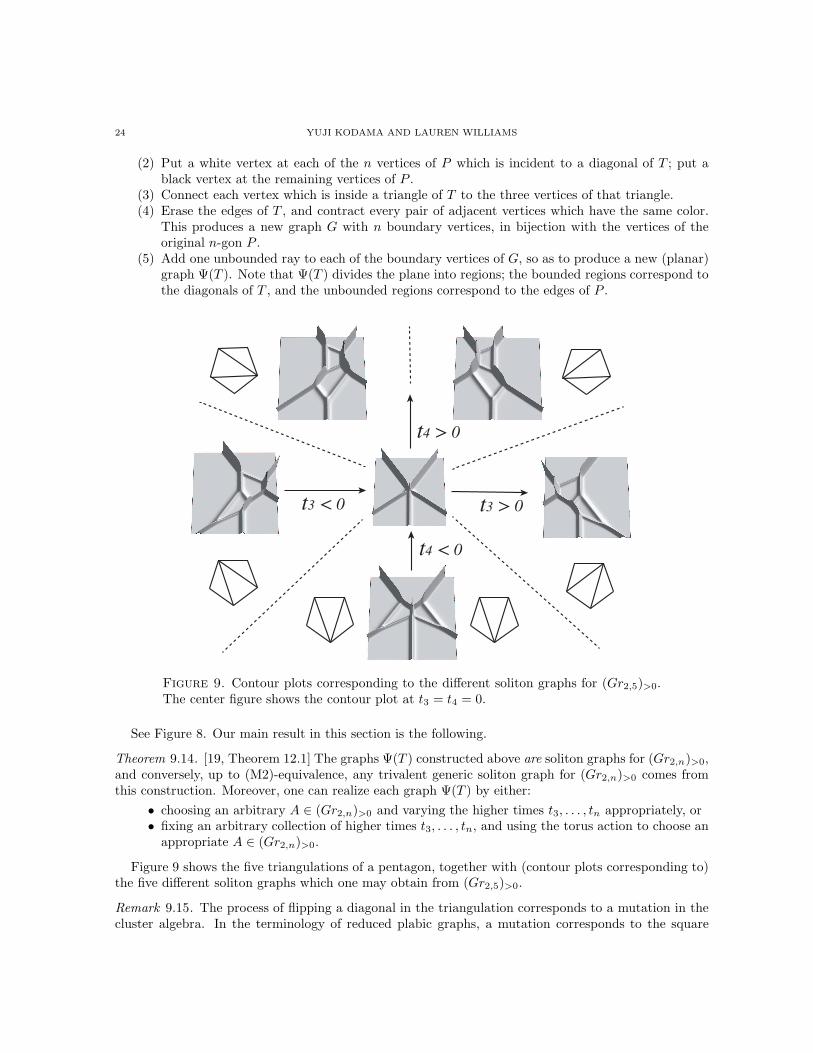
Figure 9. Contour plots corresponding to the different soliton graphs for (Gr2,5)>0.The center figure shows the contour plot at t3 = t4 = 0.
See Figure 8. Our main result in this section is the following.
Theorem 9.14. [19, Theorem 12.1] The graphs Ψ(T ) constructed above are soliton graphs for (Gr2,n)>0,and conversely, up to (M2)-equivalence, any trivalent generic soliton graph for (Gr2,n)>0 comes fromthis construction. Moreover, one can realize each graph Ψ(T ) by either:
• choosing an arbitrary A ∈ (Gr2,n)>0 and varying the higher times t3, . . . , tn appropriately, or• fixing an arbitrary collection of higher times t3, . . . , tn, and using the torus action to choose an
appropriate A ∈ (Gr2,n)>0.
Figure 9 shows the five triangulations of a pentagon, together with (contour plots corresponding to)the five different soliton graphs which one may obtain from (Gr2,5)>0.
Remark 9.15. The process of flipping a diagonal in the triangulation corresponds to a mutation in thecluster algebra. In the terminology of reduced plabic graphs, a mutation corresponds to the square
COMBINATORICS OF KP SOLITONS FROM THE REAL GRASSMANNIAN 25
move (M1). In the setting of KP solitons, each mutation may be considered as an evolution along aparticular flow of the KP hierarchy defined by the symmetries of the KP equation.
Remark 9.16. It is known already that the set of reduced plabic graphs for the TP part of Gr2,n allhave the form given by Algorithm 9.13. And by Corollary 9.9, every generic soliton graph is a reducedplabic graph. Therefore it follows immediately that every soliton graph for the TP part of Gr2,n musthave the form of Algorithm 9.13. To prove Theorem 9.14, one must also show that every outcome ofAlgorithm 9.13 can be realized as a soliton graph.
10. The inverse problem for soliton graphs
The inverse problem for soliton solutions of the KP equation is the following: given a time t togetherwith the contour plot Ct(uA) of a soliton solution, can one reconstruct the point A of Grk,n which gaverise to the solution? Note that solving for A is desirable, because this information would allow us tocompute the entire past and the entire future of the soliton solution.
Using the cluster algebra structure for Grassmannians, we have the following.
Theorem 10.1. [19, Theorem 11.2] Consider a generic contour plot Ct(uA) of a soliton solution which hasno X-crossings, and which comes from a point A of the totally positive Grassmannian at an arbitrarytime t. Then from the contour plot together with t we can uniquely reconstruct the point A.
Using the description of contour plots of soliton solutions when t≪ 0, we have the following.
Theorem 10.2. [19, Theorem 11.3] Fix κ1 < · · · < κn as usual. Consider a generic contour plot Ct(uA)of a soliton solution coming from a point A of a positroid cell Stnn
π , for t ≪ 0. Then from the contourplot together with t we can uniquely reconstruct the point A.
10.1. Non-uniqueness of the evolution of the contour plots for t≫ 0. In contrast to the totallynon-negative case, where the soliton solution can be uniquely determined by the information in thecontour plot at t≪ 0, if we consider arbitrary points A ∈ Grk,n, we cannot solve the inverse problem.
Consider A ∈ SD ⊂ Grk,n. If the contour plot C−∞(D) is topologically identical to G−(D), then thecontour plot has almost no dependence on the parameters mj from the parameterization of SD. Thisis because the Plucker coordinates corresponding to the regions of C−∞(D) (representing the dominantexponentials) are either monomials in the pi’s (see [19, Section 5] and [19, Remark 10.5]), or determinedfrom these by a “two-term” Plucker relation.
Therefore it is possible to choose two different points A and A′ in SD ⊂ Grk,n whose contour plotsfor a fixed κ1 < . . . κn and fixed t≪ 0 are identical (up to some exponentially small difference); we usethe same parameters pi but different parameters mj for defining A and A′. However, as t increases,those contour plots may evolve to give different patterns.
Consider the Deodhar stratum SD ⊂ Gr2,4, corresponding to
w = s2s3s1s2 and v = s211s2.
The Go-diagram and labeled Go-diagram are given by
②
−1 p3
p2 1.
The matrix g is calculated as g = s2y3(p2)y1(p3)x2(m)s−12 , and its projection to Gr2,4 is
A =
(
−p3 −m 1 00 p2 0 1
)
.
26 YUJI KODAMA AND LAUREN WILLIAMS
The τ -function is
τA = −(p2p3E1,2 + p3E1,4 + mE2,4 + p2E2,3 − E3,4),
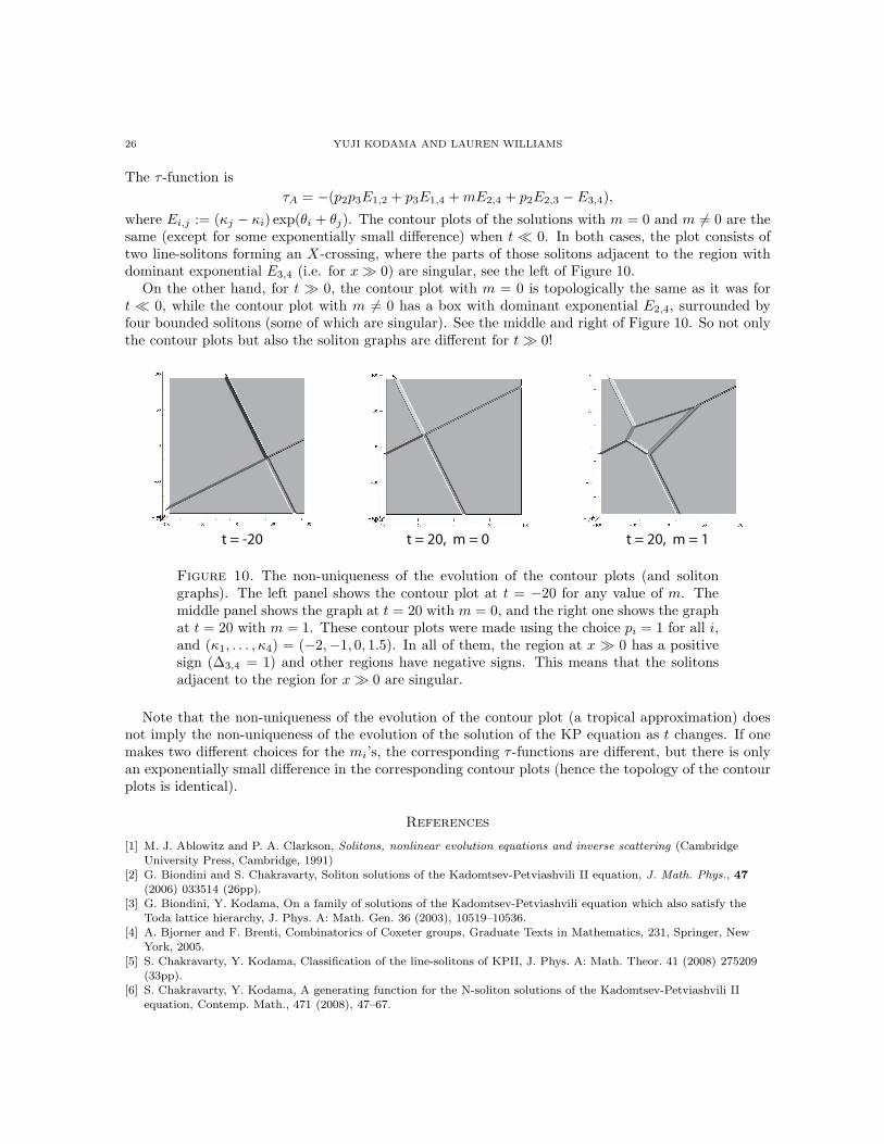
where Ei,j := (κj − κi) exp(θi + θj). The contour plots of the solutions with m = 0 and m 6= 0 are thesame (except for some exponentially small difference) when t ≪ 0. In both cases, the plot consists oftwo line-solitons forming an X-crossing, where the parts of those solitons adjacent to the region withdominant exponential E3,4 (i.e. for x≫ 0) are singular, see the left of Figure 10.
On the other hand, for t ≫ 0, the contour plot with m = 0 is topologically the same as it was fort ≪ 0, while the contour plot with m 6= 0 has a box with dominant exponential E2,4, surrounded byfour bounded solitons (some of which are singular). See the middle and right of Figure 10. So not onlythe contour plots but also the soliton graphs are different for t≫ 0!
t = -20 t = 20, m = 0 t = 20, m = 1
Figure 10. The non-uniqueness of the evolution of the contour plots (and solitongraphs). The left panel shows the contour plot at t = −20 for any value of m. Themiddle panel shows the graph at t = 20 with m = 0, and the right one shows the graphat t = 20 with m = 1. These contour plots were made using the choice pi = 1 for all i,and (κ1, . . . , κ4) = (−2,−1, 0, 1.5). In all of them, the region at x ≫ 0 has a positivesign (∆3,4 = 1) and other regions have negative signs. This means that the solitonsadjacent to the region for x≫ 0 are singular.
Note that the non-uniqueness of the evolution of the contour plot (a tropical approximation) doesnot imply the non-uniqueness of the evolution of the solution of the KP equation as t changes. If onemakes two different choices for the mi’s, the corresponding τ -functions are different, but there is onlyan exponentially small difference in the corresponding contour plots (hence the topology of the contourplots is identical).
References
[1] M. J. Ablowitz and P. A. Clarkson, Solitons, nonlinear evolution equations and inverse scattering (CambridgeUniversity Press, Cambridge, 1991)
[2] G. Biondini and S. Chakravarty, Soliton solutions of the Kadomtsev-Petviashvili II equation, J. Math. Phys., 47
(2006) 033514 (26pp).[3] G. Biondini, Y. Kodama, On a family of solutions of the Kadomtsev-Petviashvili equation which also satisfy the
Toda lattice hierarchy, J. Phys. A: Math. Gen. 36 (2003), 10519–10536.[4] A. Bjorner and F. Brenti, Combinatorics of Coxeter groups, Graduate Texts in Mathematics, 231, Springer, New
York, 2005.
[5] S. Chakravarty, Y. Kodama, Classification of the line-solitons of KPII, J. Phys. A: Math. Theor. 41 (2008) 275209(33pp).
[6] S. Chakravarty, Y. Kodama, A generating function for the N-soliton solutions of the Kadomtsev-Petviashvili IIequation, Contemp. Math., 471 (2008), 47–67.
COMBINATORICS OF KP SOLITONS FROM THE REAL GRASSMANNIAN 27
[7] S. Chakravarty, Y. Kodama, Soliton solutions of the KP equation and applications to shallow water waves, Stud.Appl. Math. 123 (2009) 83–151.
[8] V. Deodhar, On some geometric aspects of Bruhat orderings. I. A finer decomposition of Bruhat cells, Invent. Math.79 (1985), no. 3, 499–511.
[9] L. A. Dickey, Soliton equations and Hamiltonian systems, Advanced Series in Mathematical Physics, Vol. 12, (WorldScientific, Singapore, 1991).
[10] S. Fomin, A. Zelevinsky, Cluster Algebras I: Foundations, J. Amer. Math. Soc. 15 (2002), 497-529.[11] N. Freeman, J. Nimmo, Soliton-solutions of the Korteweg-deVries and Kadomtsev-Petviashvili equations: the
Wronskian technique, Phys. Lett. A 95 (1983), 1–3.[12] R Hirota, The Direct Method in Soliton Theory (Cambridge University Press, Cambridge, 2004)[13] B. B. Kadomtsev and V. I. Petviashvili, On the stability of solitary waves in weakly dispersive media, Sov. Phys. -
Dokl. 15 (1970) 539-541.[14] D. Kazhdan and G. Lusztig, Representations of Coxeter groups and Hecke algebras, Invent. Math. 53 (1979), no. 2,
165–184.[15] D. Kazhdan and G. Lusztig, Schubert varieties and Poincare duality, Geometry of the Laplace operator (Proc.
Sympos. Pure Math., Univ. Hawaii, Honolulu, Hawaii, 1979), Proc. Sympos. Pure Math., XXXVI, Amer. Math.Soc., Providence, R.I., 1980, pp. 185–203. MR 84g:14054
[16] Y. Kodama, Young diagrams and N-soliton solutions of the KP equation, J. Phys. A: Math. Gen., 37 (2004)11169-11190.
[17] Y. Kodama, KP solitons in shallow water, J. Phys. A: Math. Theor. 43 (2010) 434004 (54pp).[18] Y. Kodama, L. Williams, KP solitons, total positivity, and cluster algebras, Proc. Natl. Acad. Sci. USA 108
(2011), no. 22, 8984–8989.[19] Y. Kodama, L. Williams, KP solitons and total positivity for the Grassmannian, arXiv:1106.0023.[20] Y. Kodama, L. Williams, A Deodhar decomposition of the Grassmannian and the regularity of KP solitons,
arXiv:1204.6446.[21] G. Lusztig, Total positivity in partial flag manifolds, Representation Theory, 2 (1998) 70-78.[22] R. Marsh and K. Rietsch, Parametrizations of flag varieties, Representation Theory, 8 (2004).[23] T. Miwa and M. Jimbo and E. Date, Solitons: differential equations, symmetries and infinite-dimensional algebras
(Cambridge University Press, Cambridge, 2000)[24] S. Novikov, S. V. Manakov, L. P. Pitaevskii and V. E. Zakharov, Theory of Solitons: The Inverse Scattering
Method, Contemporary Soviet Mathematics, (Consultants Bureau, New York and London, 1984).[25] A. Postnikov, Total positivity, Grassmannians, and networks, http://front.math.ucdavis.edu/math.CO/0609764.[26] M. Sato, Soliton equations as dynamical systems on an infinite dimensional Grassmannian manifold, RIMS
Kokyuroku (Kyoto University) 439 (1981), 30–46.[27] J. Satsuma, A Wronskian representation of N-soliton solutions of nonlinear evolution equations, J. Phys. Soc.
Japan, 46 (1979) 356-360.[28] J. Scott, Grassmannians and cluster algebras, Proc. London Math. Soc. (3) 92 (2006), 345–380.[29] J. Stembridge, On the Fully Commutative Elements of Coxeter Groups. J. Algebraic Combinatorics 5 (1996),
353–385.
Department of Mathematics, Ohio State University, Columbus, OH 43210
E-mail address: [email protected]
Department of Mathematics, University of California, Berkeley, CA 94720-3840
E-mail address: [email protected]