Embed Size (px)
Citation preview

Combinatorics
Prof. A.G. Thomason
Michaelmas 2007
LATEXed by Sebastian Pancratz

ii
These notes are based on a course of lectures given by Prof. A.G. Thomason in Part III
of the Mathematical Tripos at the University of Cambridge in the academic year 2007�
2008.
These notes have not been checked by Prof. A.G. Thomason and should not be regarded
as o�cial notes for the course. In particular, the responsibility for any errors is mine �
please email Sebastian Pancratz (sfp25) with any comments or corrections.

Contents
1 Antichains 3
2 Saturation 7
3 Shadows 11
4 Intersecting Systems 17
5 Exact Intersections 21
6 Breathtaking Consequences 25
7 Shannon Capacity 29
8 The Lovász θ Function 33


Notation
We denote [n] = {1, . . . , n} and more generally write [m,n] = {m, . . . , n} for m,n ∈ N.Given a set X, we write P(X) = {Y : Y ⊂ X} or sometimes PX for the power set.
Further, we write X(r) = {Y ⊂ X : |Y | = r} and call a family F ⊂ PX r-uniform if
F ⊂ X(r). We say F is uniform if it is r-uniform for some r.


Chapter 1
Antichains
A family A ⊂ PX is a chain if whenever A,B ∈ A then A ⊂ B or B ⊂ A. Similarly,
A ⊂ PX is an antichain if whenever A,B ∈ A then A ⊂ B implies A = B.
1 2 3
1 2
tttt1 3 2 3
JJJJ
1
ttttt2
JJJJJttttt
3
JJJJJ
∅
IIIIIIuuuuuu
How large can a chain be? Trivially, a chain A ⊂ P[n] contains at most one element
from each [n](r) so |A| ≤ n + 1, which is realisable, e.g. ∅, {1}, {1, 2}, {1, 2, 3}, . . . , [n].
How large can an antichain be? Clearly [n](r) is an antichain of size(nr
), which is maximal
when r =⌊
n2
⌋or⌈
n2
⌉. Can we do better?
Theorem 1.1 (Sperner's Lemma). Let A ⊂ P[n] be an antichain. Then
|A| ≤(
n⌊n2
⌋).
Proof. We shall decompose P[n] into(
nbn/2c
)chains which proves the theorem since A
can meet each chain only once.
It su�ces to �nd injections from [n](r) to [n](r+1) so A 7→ B with A ⊂ B for r < n2 , and
from [n](r) to [n](r−1) so A 7→ B with A ⊃ B for r > n2 . The �rst injection corresponds
exactly to a matching of [n](r) to [n](r+1) in the bipartite graph whose vertex classes are
these two sets, with A ∈ [n](r) joined to B ∈ [n](r+1) if A ⊂ B.
Observe each A ∈ [n](r) is joined to n − r vertices in [n](r+1). Each B ∈ [n](r+1) is
joined to r + 1 vertices in [n](r). Let S be a collection of vertices in [n](r) and T be its
neighbours in [n](r+1). Counting the edges between S and T ,
|S|(n− r) = e(S, T ) ≤ |T |(r + 1),
so
|T | ≥ |S|n− r
r + 1≥ |S|.
as r < n2 . By Hall's theorem, the matching exists.
The second injection exists similarly.

4 Antichains
Remark. It is not clear from the proof whether the size(
nbn/2c
)can be achieved other
than in the obvious ways.
De�nition. Given A ⊂ [n](r) the (lower) shadow of A is
∂A = ∂−A = {B ∈ [n](r−1) : B ⊂ A for some A ∈ A}.
Lemma 1.2 (Local LYM). If A ⊂ [n](r) then
|∂A|(n
r−1
) ≥ A(nr
) .Proof. As in the proof of Theorem 1.1,
|A|r = e(A, ∂A) ≤ |∂A|(n− r + 1).
Remark. (i) Equality is attained only if A = ∅ or A = [n](r), since we can get from
A ∈ A to A′ ∈ [n](r) \ A by a sequence of removing and adding elements.
(ii) We can obtain another proof of Sperner's lemma along these lines. Pick r maximal
such that A∩ [n](r) 6= ∅. Replace A∩ [n](r) by its shadow if r > n2 . By Local LYM,
we obtain a larger antichain closer to the middle.
Theorem 1.3 (LYM, Lubell, Yamamoto, Meshalkin, 1966). Let A ⊂ P[n] be an an-
tichain. Thenn∑
r=0
|A ∩ [n](r)|(nr
) ≤ 1.
Proof. Let Ar = A ∩ [n](r) and
Br = Ar ∪ ∂Ar+1 ∪ · · · ∪ ∂n−rAn = Ar ∪ ∂Br+1.
Since A is an antichain, Ar ∩ ∂Br+1 = ∅. So
1 ≥ |B0|(n0
) =|A0|(
n0
) +|∂B1|(
n0
) ≥ |A0|(n0
) +|B1|(
n1
) =|A0|(
n0
) +|A1|(
n1
) +|∂B2|(
n1
)≥ |A0|(
n0
) +|A1|(
n1
) +|B2|(
n2
) ≥ · · · ≥n∑
r=0
|Ar|(nr
) .
Remark. Equality holds in LYM if and only if it holds in Local LYM at every step if
and only if A = [n]r for some r.
Alternative proof. Pick a random maximal chain C, i.e., a sequence A0 ⊂ A1 ⊂ · · · ⊂ An
where |Ar| = r. Given A ∈ [n](r),
P(A ∈ C) =1(nr
)and hence
P(C meets Ar) =|Ar|(
nr
) .
But for 0 ≤ r ≤ n these events are mutually exclusive, so the sum of their probabilities
is at most 1.

5
De�nition. A chain is symmetric if it is of the form
Ak ⊂ Ak+1 ⊂ · · · ⊂ An−k
for some k where Ai ∈ [n](i).
Can we decompose P[n] into symmetric chains? Note there are necessarily(
nbn/2c
)chains,
since each chain has an element of [n](bn/2c).
Theorem 1.4. P[n] has a partition into symmetric chains.
Proof. By induction on n. Take a partition of P[n − 1] into symmetric chains. Let
B = Ak, Ak+1, . . . , An−1−k be a chain in it. Let
B′ = Ak, Ak+1, . . . , An−1−k, An−1−k ∪ {n}B′′ = Ak ∪ {n}, Ak+1 ∪ {n}, . . . , An−2−k ∪ {n}
Notice that B′, B′′ are symmetric chains in P[n] and every element of P[n] is in exactly
one of these chains.
Say what now? We seem to have twice as many chains in P[n] as in P[n − 1] but(n
bn/2c)6= 2(
n−1b(n−1)/2c
)if n is odd. But in this case, n− 1 is even, B can have length one,
and then B′′ = ∅. In fact, the procedure generates
`k(n) =(
n
k
)−(
n
k − 1
)chains of length n− 2k + 1 for 0 ≤ k ≤
⌊n2
⌋because `k(n) = `k(n− 1) + `k−1(n− 1).
Littlewood and O�ord (1943) needed a bound on the number of sums∑
i∈A zi, A ⊂ [n],that lie within distance 1 of each other, where z1, . . . , zn ∈ C, |zi| ≥ 1. Erd®s (1945)
noticed if zi ∈ R then the number is at most(
nbn/2c
), since the sets A∗ = {i ∈ A : zi >
0} ∪ {i 6∈ A : zi < 0} form an antichain.
Theorem 1.5 (Kleitman, 1970). Let x1, . . . , xn ∈ X, where (X, ‖·‖) is a normed space,
with ‖xi‖ ≥ 1. For any A ⊂ [n] let xA =∑
i∈A xi. Let A ⊂ P[n] such that ‖xA−xB‖ < 1for all A,B ∈ A. Then
|A| ≤(
n⌊n2
⌋).
Proof. Call a class C ⊂ P[n] dispersed if ‖xA − xB‖ ≥ 1 for all A,B ∈ C with A 6= B. If
we can partition P[n] into(
nbn/2c
)dispersed classes, we are done.
A partition of P[n] into classes is called quasi-symmetric if it has `k(n) =(nk
)−(
nk−1
)classes of size n−2k +1, 0 ≤ k ≤ bn/2c. Notice that any such partition has
∑k `k(n) =(
nbn/2c
)classes. Notice further that the following procedure produces a quasi-symmetric
partition of P[n] from one of P[n− 1].
For each class C in the partition of P[n− 1] pick A+ ∈ C and let
C′ = C ∪ {A+ ∪ {n}}C′′ = {A ∪ {n} : A ∈ C, A 6= A+}

6 Antichains
This works because `k(n) = `k(n− 1) + `k−1(n− 1).
We need only pick A+ so that if C is dispersed, so are C′ and C′′. Notice C′′ is dispersedbecause
‖xA∪{n} − xB∪{n}‖ = ‖xA − xB‖
for A,B ∈ C′′. Let en = xn/‖xn‖ and pick A+ so that 〈xA+ , en〉 = maxA∈C〈xA, en〉.Then
‖xA+∪{n} − xA‖ ≥ 〈xA+∪{n} − xA, en〉= 〈xA+∪{n}, en〉 − 〈xA, en〉= 〈xn, en〉+ 〈xA+ , en〉 − 〈xA, en〉≥ 〈xn, en〉= ‖xn‖≥ 1.

Chapter 2
Saturation
An r-uniform hypergraph H is a pair H = (V,E) where E ⊂ V (r). A 2-uniform hyper-
graph is a graph. The complete hypergraph K(r)k of order k is ([k], [k](r)).
Recall that for r = 2, Turán's theorem tells us the maximum size, i.e., the number of
edges, of a graph with no Kk is that of the Turán graph Tk−1(n). The corresponding
value for r ≥ 3 is completely unknown, even for K(3)4 .
A hypergraph is (strongly) k-saturated if the addition of any edge not in H produces
a K(r)k subgraph. For r = 2, clearly Tk−1(n) is saturated, but there are examples with
fewer edges. E.g., for k = 3 a star will do and in general Kk−2 + En−k+2 works. Erd®s�
Hajnal�Moon (1964) showed this example has the minimum size.
Theorem 2.1 (Bollobás, 1965). Let {(Ri, Si) : i ∈ I} be a collection of pairs of subsets
of [n] such that Ri ∩ Sj = ∅ if and only if i = j. Then∑i∈I
(ri + si
ri
)−1
≤ 1
where ri = |Ri|, si = |Si|.
Remark. Putting Si = [n] − Ri, {Ri : i ∈ I} forms an antichain and we obtain the
LYM inequality.
Proof. By induction on n. The case n = 1 is trivial. For each x ∈ [n], let Ix = {i ∈ I :x 6∈ Ri}. Let Sx
j = Sj ∩ ([n]− {x}). Then by the induction hypothesis,∑i∈Ix
(ri + sx
i
ri
)−1
≤ 1.
Now Ri appears in n − ri Ix's and, of these, sxi = si − 1 in si cases, and sx
i = si in
n− ri − si cases. So
n ≥∑x∈[n]
∑i∈Ix
(ri + sx
i
ri
)−1
=∑i∈I
(n− ri − si)(
ri + si
ri
)−1
+ si
(ri + si − 1
ri
)−1
= n∑i∈I
(ri + si
ri
)−1
.

8 Saturation
Proof. Consider a random ordering of [n], i.e., a random maximal chain. Then
P(All elements of Ri precede all elements of Si) =1(
ri+siri
)and those events are mutually disjoint.
Theorem 2.2. Let H be a strongly (r + t)-saturated r-uniform hypergraph. Then
e(H) ≥(
n
r
)−(
n− t
r
)where n = |H|.
Remark. This is attained (in fact uniquely) by [n](r) − [n− t](r).
Proof. For each missing edge Ri pick a K(r)r+t created by the addition of Ri and let
Si = [n] − V (K(r)r+t). Then Ri ∩ Sj = ∅ if and only if i = j so the number of Ri is at
most(n−t
r
).
We say that H is weakly k-saturated if there is an ordering of the missing edges so that
if the edges are added one by one in that order, each additional edge creates a new K(r)k .
A strongly saturated graph is weakly saturated. The converse is false, e.g., if r = 2,k = 3 then any tree will do.
Theorem 2.3. Let H be a weakly (r + t)-saturated r-uniform hypergraph. Then
e(H) ≥(
n
r
)−(
n− t
r
)where n = |H|.
Proof. For each missing edge Ri pick Si as before. We add edges in the order R1, R2, . . . .Then Ri∩Si = ∅ and Rj∩Si 6= ∅ for j > i. The proof then follows from the Theorem 2.4.
Theorem 2.4. Let Ri, Si ⊂ [n], 1 ≤ i ≤ h with |Ri| = r, |Si| = s, Ri ∩ Si = ∅, andRj ∩ Si 6= ∅ for 1 ≤ i < j ≤ h. Then h ≤
(r+sr
).
Remark. Given a �nite dimensional vector space V with basis e1, . . . , ed, we consider
the exterior algebra∧
=⊕
k≥1
∧k V . A basis for∧k V is
ei1 ∧ ei2 ∧ · · · ∧ eik
where {i1, . . . , ik} ∈ [d](k) and we require that transposing elements results in multipli-
cation by −1; so if any two elements are equal we obtain zero. Extend this by linearity.
It is easy to check that v1 ∧ · · · ∧ vk 6= 0 i� {v1, . . . , vk} is a linearly independent set.
Proof. Let V = Rr+s, let {vx : x ∈ [n]} be vectors in general position, that is, any r + sare linearly independent. For A ⊂ [n] let vA =
∧x∈A vx. Then vA ∧ vB 6= 0 if and only
if A ∩B = ∅ and {vx : x ∈ A ∪B} is linearly independent.

9
Now vRi ∧ vSi 6= 0, but vRj ∧ vSi = 0 for i < j. Then {vRi : 1 ≤ i ≤ h} is linearly
independent, for if∑k
j=1 cjvRj = 0 let i = min{j : cj 6= 0} then(k∑
j=1
cjvRj
)∧ vSi = civRi ∧ vSi = 0
so ci = 0, contradiction. Therefore,
h ≤ dimr∧
V =(
dim V
r
)=(
r + s
r
)


Chapter 3
Shadows
Local LYM states
|∂A| ≥ |A| rn−r+1
with equality only if A = ∅ or A = [n](r). How small can |∂A| be, given |A|?If r = 1, clearly ∂A = {∅}, |∂A| = 1. If r = 2, A represents the edges of a graph. ∂A is
the set of vertices having at least one incident edge. We minimise |∂A| by
Km • m+1
d
XXXXXXXXXXXXffffffffffff
where |A| =(m2
)+ d, 0 < d ≤ m. Hence |∂A| ≥ m + 1. If d 6= m there are other
con�gurations.
The following are two important orders on [n](r). We de�ne the lexicographic (or lex )
order by A ≺ B if minA4B ∈ A, and the colexicographic (or colex ) order by A ≺ B if
max A4B ∈ B. For example, consider [5](3).
lex 123 124 125 134 135 145 234 235 245 345colex 123 124 134 234 125 135 235 145 245 345
Remark. Colex is �lex reversed on [n] reversed�.
Note if A ⊂ [n](2) then we minimised the shadow by choosing A to be an initial segment
of the colex order.
Clearly, in colex, every set with maximal element less than k precedes any set with
maximal element k. Amongst sets with maximal element k, the order is by colex on
[k − 1](r−1) + {k}.
Example. The �rst 41 elements in [n](4).
41 =(
74
)+(
43
)+(
22
)+(
11
)A = [7](4) ∪
([4](3) + {8}
)∪([2](2) + {5, 8}
)∪([1](1) + {3, 5, 8}
)∂A = [7](3) ∪
([4](2) + {8}
)∪([2](1) + {5, 8}
)∪([1](0) + {3, 5, 8}
)|∂A| =
(73
)+(
42
)+(
21
)+(
10
)= 44

12 Shadows
Observation 3.1. Each m ∈ N has, given �xed r, a unique expression
m =(
mr
r
)+(
mr−1
r − 1
)+ · · ·+
(ms
s
)where mr > mr−1 > · · · > ms ≥ s ≥ 1. If I is the initial segment of length m in the
colex order on [n](r) then
|∂I| =(
mr
r − 1
)+(
mr−1
r − 2
)+ · · ·+
(ms
s− 1
).
Observation 3.2. Let 1 ∈ A ∈ [n](r) and let B be the �rst element after A in colex
with 1 6∈ B. Then A− {1} ⊂ B.
To check this, consider the maximal string of consecutive numbers in A beginning with 1,i.e., write A = [l]∪C, l+1 6∈ A. The next elements in colex are {1, 2, . . . , l−1, l+1}∪C,
{1, 2, . . . , l − 2, l, l + 1} ∪ C, . . . , {1, 3, 4, . . . , l + 1} ∪ C, {2, 3, . . . , l + 1} ∪ C = B.
Our hope is to transform a family A to another family more like an initial segment,
without increasing the shadow. The last bit is the hard bit.
De�nition (i-j-compression). Let 1 ≤ i < j ≤ n, A ∈ [n](r) then
Cij(A) =
{A− {j} ∪ {i} if j ∈ A, i 6∈ A
A otherwise.
For A ⊂ [n](r) its i-j-compression is
CijA = {Cij(A) : A ∈ A} ∪ {A ∈ A : Cij(A) ∈ A}
replacing sets A by their compression if possible.
Example.
C12{125, 146, 156, 256, 257, 357} = {125, 146, 156, 256, 157, 357}
Clearly, |CijA| = |A|.
Lemma 3.3.
|∂CijA| ≤ |∂A|
Proof. We consider the injection P[n] → P[n], B 7→ B4{i, j} and show it maps ∂CijA\∂A to ∂A \ ∂CijA, proving the lemma.
Let B ∈ ∂CijA \ ∂A. Then there exists A ∈ A with B ⊂ Cij(A) with Cij(A) 6∈ A so
Cij(A) 6= A. Then A = Z ∪ {j}, Cij(A) = Z ∪ {i}, Z ∈ [n](r−1), i, j 6∈ Z.
Now B 6= Z since B 6∈ ∂A, so B = Z−{k}∪{i}, k ∈ Z. So B 7→ B′ = Z−{k}∪{j} ⊂ A,so B′ ∈ ∂A.Suppose B′ ∈ ∂CijA, i.e., B′ ⊂ A′ ∈ CijA. Then A′ = B′ ∪ {l} = Z − {k} ∪ {j} ∪ {l}.If l = i then A′ ∈ A and B ⊂ A′ so B ∈ ∂A, contradiction. But if l 6= i then
A′ = Z − {k} ∪ {j} ∪ {l} can be in CijA only if Cij(A′) = Z − {k} ∪ {i} ∪ {l} ∈ A. SoB ⊂ CijA
′, i.e., B ∈ ∂A, contradiction.Hence B′ 6∈ ∂CijA, completing the proof.

13
We say A is i-j-compressed if CijA = A. We say A is left-compressed if CijA = A for
all i < j.
Corollary 3.4. Given A ⊂ [n](r) there exist B ⊂ [n](r) with |B| = |A|, |∂B| ≤ |∂A| andB is left-compressed.
Proof. If CijA 6= A replace A by CijA. This reduces∑
A∈A∑
i∈A i. Keep doing this;
since the quantity is positive we reach a left-compressed family B, which has the desired
properties by Lemma 3.3.
An initial segment of colex is left-compressed but unfortunately there are many more
other examples, e.g., an initial segment of lex. Nevertheless, we have enough for our
main theorem.
Theorem 3.5 (Kruskal�Katona, 1963�1968). Let A ⊂ [n](r) and let J be the initial
segment of colex on [n](r) with |A| = |J |. Then |∂A| ≥ |∂J |. Explicitly, if
|A| = m =(
mr
r
)+(
mr−1
r − 1
)+ · · ·+
(ms
s
)where mr > mr−1 > · · · > ms ≥ s ≥ 1, then
|∂A| ≥(
mr
r − 1
)+ · · ·+
(ms
s− 1
).
Proof. Proceed by induction on m + r. By Corollary 3.4, we may assume A is 1-j-compressed for all 1 < j. Let us de�ne
A1 = {A− {1} : 1 ∈ A ∈ A} J1 = {A− {1} : 1 ∈ A ∈ J }A2 = {A ∈ A : 1 6∈ A} J2 = {A ∈ J : 1 6∈ A}
Notice that J1 is an initial segment of colex on {2, . . . , n}(r−1) and J2 is an initial
segment of colex on {2, . . . , n}(r). Then |A| = |A1|+ |A2| and |J | = |J1|+ |J2|.
Now A is 1-j-compressed means ∂A2 ⊂ A1. Thus ∂A = A1 ∪ ({1}+ ∂A1) is a partitionof ∂A. So |∂A| = |A1|+ |∂A1|, and likewise |∂J | = |J1|+ |∂J1|.
So we are home by induction if |A1| ≥ |J1|. What if |A1| < |J1|? Then |A2| > |J2|.Let J +
2 be J2 plus the next element in colex on {2, . . . , n}(r). Then J +2 is an initial
segment of colex and |A2| ≥ |J +2 |. Then J1 ⊂ ∂J +
2 by Observation 3.2.
But, recalling ∂A2 ⊂ A1, we now obtain |A1| ≥ |∂A2| ≥ |∂J +2 | ≥ |J1| using the
induction hypothesis, contradiction.
Theorem 3.6. Let A ⊂ [n](r) with |A| =(xr
)where x > r − 1 then
|∂A| ≥(
x
r − 1
).
Proof (Lovász 1979). By Theorem 3.5.

14 Shadows
Proof (Frankl 1984). Since(
xr−1
)is increasing for x > r− 1 and |A| ≥ 1 we have x ≥ r.
Moreover, if x = r the result is trivial so we may assume x > r.
Proceed as in the proof of Theorem 3.5; A is 1-j-compressed, ∂A2 ⊂ A1 and |A| =|A1| + |A2|, |∂A| = |A1| + |∂A1|. If |A1| ≥
(x−1r−1
)then |∂A1| ≥
(x−1r−2
)by induction so
|∂A| ≥(
xr−1
). If |A1| <
(x−1r−1
)then |A2| >
(x−1
r
)and since x > r, induction shows
|∂A2| ≥(x−1r−1
)> |A1|, contradicting ∂A2 ⊂ A1.
An initial segment of lex is left-compressed. But we could move 125 to 234 using C34,15.
Given U, V ⊂ [n], U ∩ V = ∅ and A ⊂ [n] we de�ne
CUV (A) =
{(A \ V ) ∪ U if V ⊂ A and U ∩A = ∅A otherwise
and
CUVA = {CUV (A) : A ∈ A} ∪ {A ∈ A : CUV (A) ∈ A}
Note C{i}{j} = Cij and |CUVA| = |A|. If A ⊂ [n](r) and |U | = |V | then CUVA ⊂ [n](r).But note that
A = {14, 15} ∂A = {1, 4, 5}C23,14A = {23, 15} ∂C23,14A = {1, 2, 3, 5}
However, we have the following lemma.
Lemma 3.7 (Bollobás�Leader, 1987). Let A ⊂ [n](r), U ∩ V = ∅, |U | = |V |. Suppose
∀u ∈ U ∃v ∈ V CU−{u},V−{v}A = A (†)
Then |∂CUVA| ≤ |∂A|.
Proof. We show that the bijection of P[n] → P[n] given by Y 7→ Y 4 (U ∪ V ) injects∂A′ \ ∂A into ∂A \ ∂A′ where ·′ denotes CUV ·.
Let B ∈ ∂A′ \∂A. So there exists x ∈ [n] such that B∪{x} ∈ A′ \A. Thus U ⊂ B∪{x}and V ∩ (B ∪ {x}) = ∅. Thus (B ∪ {x} \ U) ∪ V ∈ A. Now x 6∈ U , else by (†)there exists v ∈ V with CU−{u},V−{v}(B ∪ {x} \ U) ∪ V = B ∪ {v} ∈ A, implying
B ∈ ∂A. Thus x 6∈ U ∪ V , so B 4 (U ∪ V ) = (B \ U) ∪ V ∈ ∂A. Suppose that
(B \ U) ∪ V ∈ ∂A′. Then there exists y such that (B \ U) ∪ V ∪ {y} ∈ A′. Suppose
y 6∈ U . Then B ∪ {y} = CUV (B \ U) ∪ V ∪ {y} ∈ A, giving B ∈ ∂A, a contradiction.
Hence y ∈ U . Then by (†) there exists v ∈ V such that CU−{u},V−{v}A = A. So both
(B \U)∪ V ∪ {y} ∈ A′ and CU−{u},V−{v}(B \U)∪ V ∪ {y} = B ∪ {v} ∈ A, so B ∈ ∂A.
Thus B 4 (U ∪ V ) = (B \ U) ∪ V ∈ ∂A \ ∂A′ as claimed.
De�nition.
Γ = {(U, V ) ∈ P[n]× P[n] : U ∩ V = ∅, |U | = |V |,max U < max V }
Lemma 3.8. A is an initial segment of colex if and only if CUVA = A for all (U, V ) ∈ Γ.

15
Proof. If A is not an initial segment pick A′ 6∈ A, A ∈ A where A′ ≺ A. Let U = A′ \A,V = A \ A′. Then CUV (A) = A′, so CUVA 6= A, and max(U ∪ V ) = max(A 4 A′) ∈A ⊂ V , i.e., (U, V ) ∈ Γ.
If CUVA 6= A pick A ∈ A with CUV A 6∈ A, then max(CUV (A)4A) = max(U ∪V ) ∈ A,so CUV (A) ≺ A and A is not an initial segment.
Proof (Kruskal�Katona). Given A which is not an initial segment of colex, pick (U, V ) ∈Γ with CUVA 6= A and |U | minimal, by Lemma 3.8. By Lemma 3.7,
|∂CUVA| ≤ |∂A|.
Repeat; since the members of CUVA are to the left of those in A, we cannot repeat
forever.
What about minimising |∂+A|? This depends on n.
Corollary 3.9. Let A ⊂ [n](r) and let J be the initial segment of [n](r) in the lex order
with |A| = |J |. Then |∂+A| ≥ |∂+J |.
Proof. De�ne A = {[n] − A : A ∈ A} ⊂ [n](n−r). Then ∂+A = ∂−A; we use Kruskal�Katona and the relationship between lex and colex.


Chapter 4
Intersecting Systems
We say A ⊂ P[n] is intersecting if A ∩B 6= ∅ for all A,B ∈ A. For example, A = {A ⊂[n] : 1 ∈ A} is intersecting and |A| = 2n−1.
Proposition 4.1. If A ⊂ P[n] is intersecting then |A| ≤ 2n−1.
Proof. A can contain at most one of each pair A, [n]−A.
What about uniform intersecting systems? Note if r > n2 then [n](r) is intersecting. If
r = n2 then any choice of one from each pair A, [n] − A gives an intersecting family of
size 12
(nr
)=(n−1r−1
). If r < n
2 the family {A ∈ [n](r) : 1 ∈ A} is intersecting and has size(n−1r−1
).
Theorem 4.2 (Erd®s�Ko�Rado, 1938, 1961). Let A ⊂ [n](r) with r ≤ n2 be intersecting.
Then
|A| ≤(
n− 1r − 1
).
Proof. Let A = {[n]−A : A ∈ A} ⊂ [n](n−r). The fact that A is intersecting is precisely
the statement that A ∩ ∂n−2rA = ∅. If
|A| >(
n− 1r − 1
)then
|A| = |A| >(
n− 1r − 1
)=(
n− 1n− r
)so, by Kruskal�Katona n− 2r times,
|∂n−2rA| ≥(
n− 1r
).
But then
|A|+ |∂n−2rA| >(
n− 1r − 1
)+(
n− 1r
)=(
n
r
),
contradiction.

18 Intersecting Systems
Proof (Katona). Consider all n! cyclic orders of the n elements. A set A ∈ A appears as
an arc in n ·r! · (n−r)! orders. Given a �xed cyclic ordering at most r arcs can represent
sets in A. (If (c1, . . . , cr) is an arc in A then for 1 ≤ i ≤ r − 1 at most one of the arcs
(·, ·, . . . , ci) and (ci+1, ·, ·, . . . ) is in A.) Thus
|A| · n · r! · (n− r)! ≤ r · n!.
We say A is t-intersecting if |A ∩ B| ≥ t for A,B ∈ A. Clearly, intersecting means
1-intersecting. We consider the non-uniform case �rst.
Lemma 4.3. Let A ⊂ P[n] be t-intersecting. Then CUVA is t-intersecting provided
|U | ≥ |V | and
(i) CU,V−{v}A = A for all v ∈ V ,
(ii) for all u ∈ U there exists v ∈ V such that CU−{u},V−{v}A = A.
Proof. Suppose not. Then there exist A,B ∈ CUVA with |A∩B| < t. Clearly not both
A,B ∈ A, so we assume A = CUV A′, A′ ∈ A, A 6∈ A so A = (A′ − V ) ∪ U .
Suppose B 6∈ A. Then B = (B′ − V ) ∪ U where B′ ∈ A. Then
|A ∩B| = |(A′ − V ∪ U) ∩ (B′ − V ∪ U)| = |A′ ∩B′|+ |U | − |V | ≥ t
contradiction. So B ∈ A. Suppose CUV B 6= B. Then CUV B ∈ A since B ∈ CUVA. So
|A ∩B| = |(A′ − V ∪ U) ∩B| = |A′ ∩ (B − V ∪ U)| = |A′ ∩ CUV B| ≥ t
contradiction. So CUV B = B. Hence either V 6⊂ B or V ⊂ B but U ∩B 6= ∅. If V 6⊂ Btake v ∈ V , v 6∈ B. By (i) CU,V−{v}A
′ ∈ A. Then
|A ∩B| = |(A′ − V ∪ U) ∩B| = |(A′ − V ∪ {v} ∪ U) ∩B| = |CU,V−{v}A′ ∩B| ≥ t
contradiction. Finally, if V ⊂ B but U ∩B 6= ∅, take u ∈ U ∩B and by (ii) take v ∈ Vso that CU−{u},V−{v}A = A. Then
|A ∩B| = |(A′ − (V − {v}) ∪ (U − {u})) ∩B| = |CU−{u},V−{v}A′ ∩B| ≥ t
since CU−{u},V−{v}A′ ∈ A.
Theorem 4.4 (Katona, 1964). Let A ⊂ P[n] be t-intersecting. Then
|A| ≤∣∣[n](≥k)
∣∣ = n∑i=k
(n
i
)
if n + t = 2k, and
|A| ≤∣∣[n](>k) ∪ [n− 1](k)
∣∣ = (n− 1k
)+
n∑i=k+1
(n
i
)
if n + t = 2k + 1.

19
Proof. Consider all pairs (U, V ) with |U | > |V |, U ∩ V = ∅. Keep choosing such a pair
with |V | minimal and CUVA 6= A, if such a pair exists. If V = ∅, CUVA is trivially t-intersecting, and if V 6= ∅ then CUVA is t-intersecting by Lemma 4.3 and the minimality
of |V |. Replace A by CUVA. This increases∑
A∈A|A| so eventually we reach a family
with CUVA = A for all pairs (U, V ).
De�ne r = min{|A| : A ∈ A}. Then [n](j) ⊂ A for all j > r: else let A ∈ A ∩ [n](r) andB ∈ [n](j) \ A, put U = B −A, V = A−B, and note CUVA 6= A.
Now pick A ∈ A ∩ [n](r) and B ∈ [n](r+1) with |A ∩B| = r + (r + 1)− n. Since B ∈ A,we have 2r + 1− n ≥ t, so r ≥ k.
If n + t is even, we are done; because A ⊂ [n](≥k) and the latter is t-intersecting. If
n + t is odd, A ⊂ [n](>k) ∪ (A∩ [n](k)) which is t-intersecting if and only if A∩ [n](k) is
t-intersecting. This condition is equivalent to |A ∪B| < n if A,B ∈ A ∩ [n](k), which is
equivalent to {[n]−A : A ∈ A ∩ [n](k)} is an intersecting (n− k)-uniform family. Since
n− k ≤ n2 , Erd®s�Ko�Rado says
|A ∩ [n](k)| ≤(
n− 1n− k − 1
)=(
n− 1k
).
Theorem 4.5. Let 1 ≤ t ≤ r and let A ⊂ [n](r) be t-intersecting. If n is su�ciently
large, e.g., n ≥ (16r)r, then
|A| ≤(
n− t
r − t
).
Proof. We may assume t < r and A is maximal t-intersecting. Then we may choose
A,B ∈ A with |A ∩B| = t.
If Y ⊃ A ∩B for all Y ∈ A then
|A| ≤(
n− t
r − t
)So suppose there exists C ∈ A with A∩B 6⊂ C. Thus, if D ∈ A then |D∩(A∪B∪C)| ≥t + 1. Thus
|A| ≤ 2|A∪B∪C|[(
n
r − t− 1
)+(
n
r − t− 2
)+ · · ·+
(n
0
)]<
(n− t
r − t
)if n is large.
Theorem 4.5 fails if n is not large. Let
Fi = {A ∈ [n](r) : |A ∩ [t + 2i]| ≥ t + i}.
These are t-intersecting families, interpolating between two con�gurations.
Example. Let r = 4 and t = 2.

20 Intersecting Systems
n |F0| |F1| |F2|
7(52
)= 10 1 +
(43
)(31
)= 13
(64
)= 15
8(62
)= 15 1 +
(43
)(41
)= 17
(64
)= 15
9(72
)= 21 1 +
(43
)(51
)= 21
(64
)= 15
Frankl (1987) conjectured one of Fi always wins. In particular, F0 is biggest if n >(r−t+1)(t+1), which was proved by Wilson in 1984 (c.f. Theorem 4.5). The conjecture
was proved by Ahlswede and Khachatrian in 1997.
There remain many beautiful open problems. These two are both due to Simonovits
and Sós.
(i) If A ⊂ P[n] such that |A ∩ B| contains a 3-term arithmetic progression, then
|A| ≤ 2n−3.
(ii) If A ⊂ P[n] is a family of graphs on the vertex set [n] such that |A ∩B| containsa triangle then |A| ≤ 2(n
2)−3. It is known that |A| ≤ 2(n2)−2.

Chapter 5
Exact Intersections
Historical notes from statistics: a (r, k)-λ design is a family A ⊂ [v](r) for some v, whosemembers are called blocks, every element of [v] lies in exactly k blocks, and every pair
of elements of [v] lies in λ blocks.
Clearly, the parameters are constrained. For example, if b = |A| then br = vk and
λ(v2
)= b(r2
). A less apparent constraint is b ≥ v, called Fisher's Inequality. It turns out
to hold more generally: we need only A ⊂ P[v] with every pair in [v] lying in λ blocks.
The dual system to A is A∗ = {Ax : x ∈ [v]} where Ax = {A ∈ A : x ∈ A}. Think of
a bipartite graph with vertex class [v] and A with edges representing containment. The
dual version of Fisher is the one we shall prove.
Theorem 5.1 (Fisher's Inequality). Let A ⊂ P[n] and let λ ∈ N ∪ {0} be such that
|A ∩B| = λ for distinct A,B ∈ A. Then |A| ≤ n, unless λ = 0 then |A| ≤ n + 1.
Proof. If |A| = λ for some A ∈ A then B ⊃ A for all B ∈ A and the sets B \ A are
pairwise disjoint, so |A| ≤ 1 + n− |A|.So we may assume |A| > λ for all A ∈ A. For A ∈ A let xA ∈ Rn be its characteristic
vector, i.e. xA = (δ1, . . . , δn) where δi = 1 if i ∈ A and δi = 0 if i 6∈ A. Then xA·xA = |A|,and xA · xB = |A ∩B| = λ if A 6= B.
Suppose now∑
A∈A cAxA = 0 where cA ∈ R. Then dotting with xB we obtain
cB(|B| − λ) = −λC
for C =∑
A∈A cA. If λ = 0 this implies cB = 0 for all B ∈ A. If λ 6= 0 then cB has the
opposite sign to∑
A∈A cA, a contradiction unless cB = 0 for all B ∈ A.Either way, the xA are linearly independent so |A| ≤ n.
What if we allow more than one intersection size?
Theorem 5.2. Let L ⊂ N∪{0} and let A ⊂ [n](r) be such that |A∩B| ∈ L for distinct
A,B ∈ A. Suppose gcd(L) - r. Then |A| ≤ n.
Proof. Let xA ∈ Qn be the characteristic vector of A ∈ A. Then there exists integers jA
with∑
A∈A jAxA = 0 with gcd{jA : A ∈ A} = 1.
Take a prime power pk with pk | l for all l ∈ L but pk - r. Dotting with xB gives∑A∈A
jA|A ∩B| = 0.

22 Exact Intersections
Hence pk | jB|B| for all B. Thus p | jB, contradicting gcd{jA : A ∈ A} = 1.
More generally, A can be bigger. If all we know is that |L| = s then [n](s) and [n](≤s) are
examples of uniform and non-uniform families of sizes(ns
)and
(n0
)+· · ·+
(ns
), respectively.
These bounds are in fact tight: proved by Ray�Chaudhuri and Wilson (uniform case,
1975) and Babai (non-uniform case, 1980's).
Theorem 5.3. Let L ⊂ N ∪ {0}, |L| = s. Let A ⊂ P[n] with |A ∩ B| ∈ L for distinct
A,B ∈ A. Then
|A| ≤(
n
0
)+ · · ·+
(n
s
).
Proof. For A ∈ A de�ne the polynomial fA : Rn → R by
fA(x) =∏l∈L
l<|A|
(〈x, xA〉 − l)
where x = (x1, . . . , xn) and 〈x, xA〉 = δ1x1 + · · ·+ δnxn. Note fA(xB) = 0 unless A ⊂ B.
Let fA be the polynomial obtained from fA by replacing all powers xei , e ≥ 2, by xi.
Then fA(xB) = 0 unless A ⊂ B, because fA(xB) = fA(xB) as xB ∈ {0, 1}n.
Suppose∑
A∈A cAfA(x) = 0. Pick B with |B| minimal and cB 6= 0. Then∑A∈A
cAfA(xB) = cB fB(xB) 6= 0
a contradiction. So the fA are linearly independent.
The fA are spanned by all monomials∏
i∈T xi where T ⊂ [n](≤s). Hence
|A| ≤ |[n](≤s)|
A long-standing conjecture that |A| ≤∑s
i=0
(n−1
i
)if 0 6∈ L, achievable by {Y ∈
[n](≤s+1) : 1 ∈ Y }, was proved by Snerily (2003). Compare this with Fisher's Inequality.
Why not replace the underlying �eld in the proof by GL(p)?
We use the notation m ∈ L (mod p) if there exists l ∈ L with m ≡ l (mod p), m 6∈ L(mod p) means that for all l ∈ L we have m 6≡ l (mod p).
Theorem 5.4. Let p be a prime. Let L ⊂ N ∪ {0}, |L| = s. Let A ⊂ P[n] such that
|A| 6∈ L (mod p) for all A ∈ A but |A ∩B| ∈ L (mod p) for distinct A,B ∈ A. Then
|A| ≤(
n
0
)+ · · ·+
(n
s
).
Proof. Repeat the proof of Theorem 5.3 but over GL(p) instead of R and with
fA(x) =∏l∈L
(〈xA, x〉 − l).
Then fA(xA) 6= 0 but fA(xB) = 0 for all B 6= A so the fA (and the fA) are linearly
independent.

23
The following �uniform� version uses a di�erent proof.
Theorem 5.5 (Frankl�Wilson, 1981). Let p be a prime number, let L ⊂ N ∪ {0},|L| = s, suppose r ∈ N is such that r 6∈ L (mod p). Let A ⊂ P[n] be such that |A| ≡ r(mod p) for all A ∈ A and |A ∩B| ∈ L (mod p) for distinct A,B ∈ A.Suppose moreover that r 6∈ {0, 1, . . . , s− 1} (mod p). Then
|A| ≤(
n
s
).
Remark. The condition r 6∈ {0, 1, . . . , s− 1} (mod p) is an artefact of the proof. With
more work it can be replaced by say r + s < n.
Proof. Let Ai and Mi, 0 ≤ i ≤ s, be the |A| ×(ni
)and the
(ns
)×(ni
)matrices whose
rows are indexed by A and [n](s) and whose columns are indexed by [n](i). The entry in
row A and column B is 1 if A ⊃ B and 0 if A 6⊃ B.
Let V be the vector space over GL(p) spanned by the columns of As. Then dim V ≤(ns
).
Note that if M is any(ns
)× t matrix then the columns of AsM are in V .
Let A ∈ A and I ∈ [n](i). Then
(AsMi)AI = |{S ∈ [n](s) : A ⊃ S ⊃ I}|
which is 0 if I 6⊂ A and(|A|−i
s−i
)if I ⊂ A. Thus AsMi ≡
(r−is−i
)Ai (mod p). By the
condition,(r−is−i
)6≡ 0 (mod p), so the columns of Ai are in V .
Thus the columns of Bi = AiATi are in V . This is an |A| × |A| matrix whose (A,B)
entry is |{I ∈ [n](i) : I ⊂ A, I ⊂ B}| =(|A∩B|
i
).
Consider the polynomial
φ(x) =∏l∈L
(x− l).
Then φ(r) 6= 0 but φ(l) = 0 for all l ∈ L over GF (p). Take scalars c0, . . . , cs so
φ(x) = c0
(x
0
)+ · · ·+ cs
(x
s
).
Let B = c0B0 + · · ·+ csBs. The (A,B) entry of B is φ(|A ∩ B|). So B is zero (mod p)o�-diagonal and non-zero on-diagonal. So B is non-singular and its columns are in V .
Hence
|A| = rankB ≤ dim V ≤(
n
s
).
Corollary 5.6 (Ray�Chaudhuri, Wilson, 1975). Let A ⊂ [n](r) and let L = {|A ∩ B| :A,B ∈ A, A 6= B}. Then
|A| ≤(
n
|L|
).
Proof. Clearly, r 6∈ L and r ≥ s = |L|. Choose a prime greater than r and apply
Theorem 5.5.
We might ask whether Theorem 5.5 holds for non-primes p. Here is a special case.

24 Exact Intersections
Theorem 5.7. Let q < r be a prime power. Let A ⊂ [n](r) be such that |A ∩ B| 6≡ r(mod q) for distinct A,B ∈ A. Then
|A| ≤(
n
q − 1
).
Proof. Copy the previous proof but work over Q. Then AsMi =(r−is−i
)Ai so the columns
of Ai are in V over Q. Let φ(x) =(r−1−x
q−1
)and choose c0, . . . , cs with
φ(x) =s∑
i=0
ci
(x
i
)where s = q − 1. Then the (A,B) entry in B is φ(|A ∩B|).If A = B the entry is φ(r) =
( −1q−1
)= (−1)q−1 6≡ 0 (mod p) where q is a power of p. On
the other hand, the identity
(r − l)φ(l) = q
(r − l
q
)is an identity in four integers and if r − l 6≡ 0 (mod q) then φ(l) ≡ 0 (mod p). So B is
non-singular.
Does Frankl�Wilson hold for non-prime moduli? Do we still obtain a polynomial bound,
if s is �xed?
Grolmusz (2000) gave examples where this fails. There exists a uniform family A ⊂ [n](r)
where r ≡ 0 (mod 6) and |A ∩B| 6≡ 0 (mod 6) for distinct A,B ∈ A and
|A| = exp{(
127 + o(1)
) log2 n
log log n
}In this example, r ≈ n1− 1
27 .

Chapter 6
Breathtaking Consequences
The graph on Rn has points of Rn as vertices and edges joining points at distance 1.What is χ(Rn)? If n = 2, we know 4 ≤ χ(R2) ≤ 7. In general, χ(Rn) ≤ 3n by tiling Rn
with cubes. A compactness argument by Erd®s and de Bruyn shows that there exist a
�nite subgraph H with χ(H) = χ(Rn).
Corollary 6.1 (Frankl�Wilson, 1981).
χ(Rn) ≥ (1.2 + o(1))n.
Proof. Let G be the subgraph spanned by
V ={
1√2q
xA : A ⊂ [n](2q−1)
}.
Then two points in V are distance 1 apart if and only if |A∩B| = q− 1. If q is a prime
or a prime power then no colour can be used more than(
nq−1
)times by Theorem 5.7.
Hence
χ(G) ≥(
n2q−1
)(n
q−1
) .
Take q = (2−√
2 + o(1))n4 and q prime.
Even older and more famous is Borsuk's Conjecture: every set of diameter 1 in Rn is
the union of n + 1 sets of diameter less than 1. This is true if n = 3, and if the sets are
smooth or centrally symmetric.
Corollary 6.2 (Kahn�Kalai, 1993). There is a set in Rn of diameter 1 that is not the
union of 1.2√
n sets of diameter less than 1.
Proof. Choose m = 4q with(m2
)≈ n. Think of the coordinates of Rn as being the edges
of the complete graph [m](2).
For each subset A ∈ [m](m/2) let vA be the characteristic vector of the edges between Aand [m] − A. So vA and v[m]−A are equal; they have 4q2 ones. If A,B are two subsets
then
d2(vA, vB) = 4i(2q − i)

26 Breathtaking Consequences
where i = |A ∩B|.
i
2q−i
2q−i
i
A [m]−A
B
[m]−B
Thus d2(vA, vB) ≤ 4q2 with equality if and only if |A ∩B| = q. Let
S ={
12q
vA : 1 ∈ A ∈ [m](m/2)
}.
Then diam(S) = 1 and |S| = 12
(m
m/2
). But if T ⊂ S has diameter less than 1 then
|A ∩B| 6= q for vA, vB ∈ 2qT . Let
A = {A− 1 : vA ∈ 2qT}.
Then |A′∩B′| 6= q−1 for A′, B′ ∈ A. Also A ⊂ [m](2q−1). By Theorem 5.7, |T | = |A| ≤(m−1q−1
). Then
|S||T |
≥12
(m
m/2
)(m−1q−1
)=
2(
mm/2
)(m
m/4
)≥ (1.14 + o(1))m
≥ 1.2√
n
Recall that the simplest non-trivial case of Ramsey's theorem asserts the existence of a
number R(t), the smallest n such that every colouring of the edges of Kn with red and
blue yields a monochromatic Kt.
It is easily shown that
R(t) ≤(
2t− 2t− 1
)≤ 22t.
Erd®s showed√
2tby means of an existential proof. We would like an explicit colouring.
It is trivial to colour K(t−1)2 with no monochromatic Kt so R(t) ≥ (t−1)2 constructively.But better polynomial bounds can be achieved.
Achieving super-polynomial bounds is trickier. Let G be the colouring of KN where
N =(nr
)where vertices are [n](r) and AB is red if |A ∩B| 6≡ −1 (mod q). There q is a
prime power and r > q is chosen with r ≡ −1 (mod q). Theorem 5.7 shows G has no
red Kt if t >(
nq−1
). If we take r = q2 − 1 then by Corollary 5.6 there is no blue Kt if
t >(
nq−1
).

27
Corollary 6.3. This construction shows
R(t) ≥ exp{(
14
+ o(1))
log2 t
log log t
}.
Proof. Take n = q3.
This remains the best known �construction�.
Remark. We could have used our non-uniform bounds to obtain essentially the same
result. The following example is due to Alon. Let p, q be two primes, r = pq − 1,N =
(nr
). Colour KN on [n](r) by AB red if |A∩B| 6≡ −1 (mod q). Then there is no red
Kt with t >(
nq−1
)+ · · ·+
(n0
)by Theorem 5.4 or with t >
(n
q−1
)by Theorem 5.5. There
is no blue Kt if t >(
np−1
)+ · · ·+
(n0
)by Theorem 5.3 or t >
(n
p−1
)by Corollary 5.6.
The bipartite Ramsey number BR(t) is the smallest N such that every red and blue
colouring or the edges of the complete bipartite graph KN,N contains a monochromatic
Kt,t. It is easy to show that √2
t< BR(t) ≤ t2t.
A �good� colouring of KN,N yields a �good� colouring of KN by identi�cation of pairs,
but the converse fails.
Until recently, the best known bipartite colouring was trivial BR(t) ≥ t2. Barak�Rao�Shealtiel�Wigderson (2006) showed
BR(t) ≥ exp((log t)ω(t)
)where ω(t) → ∞. The proof gives an algorithm which decides, for each edge in KN,N ,
whether to colour it red or blue in polynomial time. Is this a construction?

Chapter 7
Shannon Capacity
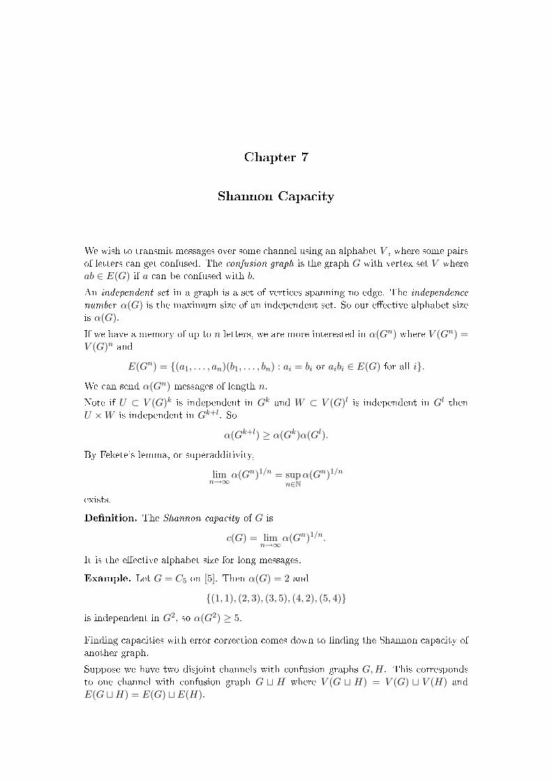
We wish to transmit messages over some channel using an alphabet V , where some pairs
of letters can get confused. The confusion graph is the graph G with vertex set V where
ab ∈ E(G) if a can be confused with b.
An independent set in a graph is a set of vertices spanning no edge. The independence
number α(G) is the maximum size of an independent set. So our e�ective alphabet size
is α(G).
If we have a memory of up to n letters, we are more interested in α(Gn) where V (Gn) =V (G)n and
E(Gn) = {(a1, . . . , an)(b1, . . . , bn) : ai = bi or aibi ∈ E(G) for all i}.
We can send α(Gn) messages of length n.
Note if U ⊂ V (G)k is independent in Gk and W ⊂ V (G)l is independent in Gl then
U ×W is independent in Gk+l. So
α(Gk+l) ≥ α(Gk)α(Gl).
By Fekete's lemma, or superadditivity,
limn→∞
α(Gn)1/n = supn∈N
α(Gn)1/n
exists.
De�nition. The Shannon capacity of G is
c(G) = limn→∞
α(Gn)1/n.
It is the e�ective alphabet size for long messages.
Example. Let G = C5 on [5]. Then α(G) = 2 and
{(1, 1), (2, 3), (3, 5), (4, 2), (5, 4)}
is independent in G2, so α(G2) ≥ 5.
Finding capacities with error correction comes down to �nding the Shannon capacity of
another graph.
Suppose we have two disjoint channels with confusion graphs G, H. This corresponds
to one channel with confusion graph G t H where V (G t H) = V (G) t V (H) and
E(G tH) = E(G) t E(H).

30 Shannon Capacity
Lemma 7.1.
c(G tH) ≥ c(G) + c(H).
Proof. Exercise.
Shannon (1956) conjectured that equality holds. Alon (1998) showed the conjecture is
utterly false. A crucial decision is to take H = G, because of the next lemma.
Lemma 7.2. Let n = |G| = |G| then
c(G t G) ≥√
2n.
Proof. Label G as a1, . . . , an and G as b1, . . . , bn where aiaj ∈ E(G) if and only if
bibj 6∈ E(G). Then
{(ai, bi) : 1 ≤ i ≤ n} ∪ {(bi, ai) : 1 ≤ i ≤ n}
is an independent set of size 2n in (G t G)2 so
c(G t G) ≥√
α((G t G)2) ≥√
2n.
To �nd a counterexample we need a graph G with both α(G) and α(G) small. This is the
Ramsey problem and random graphs give excellent examples. But no-one can bound the
capacity of random graphs su�ciently from above. Our construction of Ramsey graphs
might work. The simplest construction was based on Theorem 5.3.
Let F be a �eld and M a subspace of F [X1, . . . , Xr], the space of polynomials in rvariables over F . A representation of a graph G over M is an assignment to each vertex
u ∈ V (G) of a polynomial fu ∈ M and a vector cu ∈ F r such that fu(cu) 6= 0 and
fu(cv) = 0 for all distinct u, v ∈ V (G) with uv 6∈ E(G).
Lemma 7.3. If G has a representation over M then α(G) ≤ dim M .
Proof. If U = {u1, . . . , uα} is an independent set in G, and if∑λifui = 0
then ∑λifui(cuj ) = λjfuj (cuj )
so λj = 0 for all j. So {fu1 , . . . , fuα} is a linearly independent subset of M .
The usefulness of this idea hangs on the next lemma.
Lemma 7.4. If G has a representation over M and H has a representation over N ,
both over the same �eld F , then G ·H has a representation over M ⊗N , so
α(G ·H) ≤ dim M dim N.
Here G ·H has vertex set V (G)× V (H) and
E(G) = {(a, b)(a′, b′) : a′ = a or aa′ ∈ E(G), b′ = b or bb′ ∈ E(H)}.

31
Proof. Let M ⊂ F [X1, . . . , Xr] and N ⊂ F [Y1, . . . , Ys]. Let {gu, cu : u ∈ V (G)} repre-
sent G and {hv, dv : v ∈ V (H)} represent H. For (u, v) ∈ V (G ·H) let
f(u,v)(X1, . . . , Xr, Y1, . . . , Ys) = gu(X1, . . . , Xr)hv(Y1, . . . , Ys).
Clearly the polynomials f(u,v) lie in F [X1, . . . , Xr, Y1, . . . , Ys], in a subspace of dimension
at most dim M dim N .
Moreover (cu, dv) ∈ F r+s. Then the set
{f(u,v), (cu, dv) : (u, v) ∈ V (G ·H)}
represents G ·H since f(u,v)(cu′ , dv′) = gu(cu′)hv(dv′) and this is not 0 if (u, v) = (u′, v′)but 0 if (u, v)(u′, v′) 6∈ E(G ·H).
Corollary 7.5. If G has a representation over M then
c(G) ≤ dim M.
Proof. By Lemma 7.4, α(Gn) ≤ (dim M)n.
How can we apply this to G t G? Note that G · G is a graph of order |G|2 with an
independent set of size |G|, so Lemma 7.4 says if we can represent G, G by M,N over
the same �eld F then dim M dim N ≥ n so dim M+dim N ≥ 2√
n, so we cannot disproveShannon's conjecture this way.
Try di�erent �elds. Let p, q be distinct primes and r = pq − 1. Let G be the graph
on vertex set [n](r) where AB ∈ E(G) if |A ∩ B| ≡ −1 (mod p). Let M be the space
of multilinear polynomials in variables X1, . . . , Xn of total degree at most p − 1 over
GF (p). Then
dim M ≤(
n
0
)+ · · ·+
(n
p− 1
).
Let N be the corresponding space with p replaced by q.
Lemma 7.6. G is representable over M .
Proof. For A ∈ [n](r) let xA be its characteristic vector and
fA(x) =p−2∏j=0
(〈x, xA〉 − j)
over GF (p). Let fA ∈ M be as in the proof of Theorem 5.3. Then {fA, xA : A ∈ V (G)}represents G over M .
Lemma 7.7. G is representable over N .
Proof. Let
gA(x) =q−2∏j=0
(〈x, xA〉 − j)
over GF (q). If AB 6∈ E(G) then |A ∩ B| ≡ −1 (mod p); thus |A ∩ B| 6≡ −1 (mod q),else |A ∩ B| ≡ −1 (mod pq) so A = B. Thus {gA, xA : A ∈ [n](r)} represents G over
N .

32 Shannon Capacity
Theorem 7.8 (Alon, 1998). For each t ∈ N there exists a graph G with c(G), c(G) ≤ tand
c(G t G) ≥ exp{(
18
+ o(1))
log2 t
log log t
}where o(1) → 0 as t →∞.
Proof. Pick primes p, q with q < p < q + o(q) and let n = p3. Let G be the graph just
constructed. Then
c(G), c(G) ≤p−1∑j=0
(n
j
)= dim M ≤ 2
(n
p− 1
)by Lemma 7.6, Lemma 7.7 and Corollary 7.5. On the other hand,
c(G t G) ≥
√2(
n
pq − 1
)by Lemma 7.2

Chapter 8
The Lovász θ Function
An orthonormal representation (ONR) of a graph G is a collection of unit vectors in
Rk, some k, one for each vertex of G, such that non-adjacent vertices have orthogonal
vectors.
The tensor product of u ∈ Rk and v ∈ Rl is the vector u⊗ v in Rkl; co-ordinate-wise, if
u = (u1, . . . , uk) and v = (v1, . . . , vl) then
u⊗ v = (u1v1, u2v1, . . . , ukv1, u1v2, u2v2, . . . , uk, v2, . . . , u1vl, u2vl, . . . , ukvl).
Notice 〈u⊗ v, u′⊗ v′〉 = 〈u, u′〉〈v, v′〉. So if G has ONR {ui} and H has ONR {vj} thenG ·H has ONR {ui ⊗ vj}.Thus, similar to before, if G is representable over Rk then α(G) ≤ k, α(Gn) ≤ kn so
c(G) ≤ k.
We can do better if all the vectors in the representation lie in similar directions. The
value of a representation is
val{ui} = minc∈Rk,‖c‖=1
maxi∈V (G)
1〈c, ui〉2
.
A vector c attaining this minimum is called a handle.
De�nition.
θ(G) = min{val{ui} : {ui} represents G}.
Lemma 8.1.
α(G) ≤ θ(G).
Proof. If {ui} is an ONR and W ⊂ V (G) is independent, then {ui : i ∈ W} is an
orthogonal system, so|W |
val{ui}≤∑i∈W
〈c, ui〉2 ≤ |c|2 = 1.
Lemma 8.2.
θ(G ·H) ≤ θ(G)θ(H).
Proof. Take ONRs {ui}, {vj} for G, H together with handles c, d.
θ(G) = maxi
1〈c, ui〉2
, θ(H) = maxj
1〈d, vj〉2

34 The Lovász θ Function
Now 〈ui ⊗ vj , ul ⊗ vm〉 = 〈ui, ul〉〈vj , vm〉 so {ui ⊗ vj} is an ONR of G ·H. Let e = c⊗ d.Then 〈e, e〉 = 〈c, c〉〈d, d〉 = 1 so e is a unit vector. Then
θ(G ·H) ≤ maxi,j
1〈e, ui ⊗ vj〉2
= maxi,j
1〈c, ui〉2
1〈d, vj〉2
= θ(G)θ(H).
Theorem 8.3. For any G, c(G) ≤ θ(G).
Proof. By Lemma 8.1, α(Gn) ≤ θ(Gn). By Lemma 8.2, θ(Gn) ≤ θ(G)n.
For over 20 years no-one knew c(C5). The best bounds were√
5 ≤ c(C5) ≤ 3.
Corollary 8.4 (Lovász, 1979).
c(C5) =√
5.
Proof. Consider an umbrella with handle c and with �ve spokes. Gradually open it till
alternate spokes are orthogonal. It is easily checked that
〈c, ui〉2 =1√5
so θ(C5) ≤√
5.