COMBINED EFFECTS OF PERTURBATIONS, RADIATION, AND OBLATENESS ON THE STABILITYOF EQUILIBRIUM POINTS IN THE RESTRICTED THREE-BODY PROBLEM

AbdulRazaq AbdulRaheem1and Jagadish Singh

Department of Mathematics, Faculty of Science, Ahmadu Bello University, Zaria, Nigeria; raz11ng@yahoo.com

Received 2005 January 25; accepted 2005 October 30

ABSTRACT

This paper investigates the stability of equilibrium points under the influence of small perturbations in the Coriolisand the centrifugal forces, together with the effects of oblateness and radiation pressures of the primaries. It is foundthat collinear points remain unstable. It is also seen that triangular points are stable for 0 � � < �c and unstable for�c � � � 1

2, where� is the critical mass parameter and depends on the above parameters. It is further observed that the

Coriolis force has a stabilizing tendency, while the centrifugal force, radiation, and oblateness of the primaries have de-stabilizing effects; the presence of any one ormore of the latter makesweak the stabilizing ability of the former. There-fore, the overall effect is that the range of stability of the triangular points decreases.

Key words: celestial mechanics — methods: n-body simulations

1. INTRODUCTION

The restricted three-body problem possesses five equilibriumpoints, two triangular and three collinear. In the linear sense, thecollinear points L1, L2, and L3 are unstable for any value of themass ratio �, and the triangular points L4 and L5 are stable ifthe mass ratio � of the finite body is less than �0 ¼ 0:03852 : : :(Szebehely 1967b), where� is the ratio of themass of the smallerprimary to the total mass of the primaries and 0 � � � 1

2. Wintner

(1941) showed that the stability of the two triangular points isdue to the existence of the Coriolis terms in the equations of mo-tion expressed in a synodic coordinate system. When Szebehely(1967a) considered the effect of a small perturbation of theCoriolisforce on the stability of the equilibrium points, keeping the cen-trifugal force constant, he established that the collinear points re-main unstable. He obtained for the stability of the triangular pointsa relationship between the critical value of the mass parameter �cand the change � in the Coriolis force:

�c ¼ �0 þ16�

3ffiffiffiffiffi69

p :

Then he concluded that the Coriolis force is a stabilizing force.Subbarao & Sharma (1975) considered the same problem withone of the primaries as an oblate spheroid and its equatorial planecoinciding with the plane of motion, and showed that the oblate-ness of the primary resulted in an increase in both the Coriolisand the centrifugal force. They established further that the rangeof linear stability of the triangular points decreases, thereby con-cluding that the Coriolis force is not always a stabilizing force.Bhatnagar & Hallan (1978) extended the work of Szebehely byconsidering the effect of perturbations � and �0 in the Coriolis andthe centrifugal forces, respectively, and found that collinear pointsremain unstable; for the triangular points they obtained the relation

�c ¼ �0 þ4 36�� 19�0ð Þ

27ffiffiffiffiffi69

p :

They inferred that the range of stability increases or decreasesdepending on whether the point (�, �0) lies in one or the other of

the two parts in which the (�, �0)-plane is divided by the line36�� 19�0 ¼ 0. Sharma (1982) studied the linear stability of thetriangular equilibrium points of the restricted three-body problemwhen the more massive primary is a source of radiation and is anoblate spheroid as well. He found that the eccentricity of the con-ditional retrograde elliptic periodic orbits around the triangularpoints at the critical mass �0 increases with an increase in the ob-lateness coefficient and the radiation force and becomes unitywhen �c ¼ 0. Simmons et al. (1985) obtained a complete solu-tion of the restricted three-body problem. They discussed the ex-istence and linear stability of the equilibrium points for all valuesof radiation pressures of both luminous bodies and all values ofmass ratios. Dankowicz (2002) took account of gravitational in-teractions with asteroids and the Sun and the radiation pressurefrom the Sun. Kunitsyn (2000, 2001) studied the stability of thetriangular and collinear points in the photogravitational three-bodyproblem.In this paper we study the combined effects of perturbations in

the Coriolis and centrifugal forces, oblateness, and radiation ofthe primaries on the stability of the equilibrium points in the re-stricted problem. The participating bodies in the classical restrictedthree-body problem are strictly spherical in shape, but in actualsituations we find that several heavenly bodies, such as Saturnand Jupiter, are sufficiently oblate. The minor planets and mete-oroids have irregular shapes. In these cases, on account of thesmall dimensions of the bodies in comparison with their distancesfrom the primaries, they are considered to be point masses, but inmany cases the dimensions of the bodies are larger than the dis-tances from their respective primaries. Thus, the above assump-tion is not justified, and the results obtained are far from a realisticapproach. The lack of sphericity, or the oblateness, of the planetcauses large perturbations from a two-body orbit. The motionsof artificial Earth satellites are examples. This enables many re-searchers to study the restricted problem by taking into accountthe shapes of the bodies.We use Ai (i ¼ 1, 2) for the oblateness coefficients of the

bigger and smaller primaries, respectively, such that 0 < AiT1(McCuskey 1963) and

A1 ¼AE2

1 � AP21

5R2; A2 ¼

AE22 � AP2

2

5R2;

1 Corresponding author.

1880

The Astronomical Journal, 131:1880–1885, 2006 March

# 2006. The American Astronomical Society. All rights reserved. Printed in U.S.A.

where AE1 and AE2 are the equatorial radii and AP1 and AP2 thepolar radii of the bigger and smaller primaries, respectively. Sincethe solar radiation pressure force Fp changes with distance by thesame law as the gravitational attraction force Fg and acts oppositeto it, it is possible that this force will lead to a reduction of theeffective mass of the massive particle. And since this reductiondepends on the properties of the particle, it is acceptable to speakabout a reduced mass. Thus, the resulting force on the particle is

F ¼ Fg � Fp ¼ Fg 1� Fp

Fg

� �¼ qFg;

where q ¼ 1� Fp /Fg, a constant for a given particle, is the massreduction factor. We denote the radiation factors as qi (i ¼ 1, 2)for the bigger and smaller primaries, respectively, and these aregiven by Fpi ¼ Fg(1� qi) such that 0 < 1� qiT1.

2. EQUATIONS OF MOTION

Let m1 and m2 be the masses of the bigger and smaller pri-maries, respectively, andm the mass of the infinitesimal body.Weassume that both primaries are oblate spheroids and radiatingas well. Let A1 and A2 denote the oblateness coefficients of thebigger and smaller primaries, respectively, such that 0 < AiT1(i ¼ 1, 2).

We introduce a synodic coordinate system (O,X, Y, Z ) with theorigin at the center of mass of the primaries, in which the axesrotate relative to the inertial space with angular velocity n aboutthe z-axis. Let (x, y) be the coordinates of the infinitesimal bodyin the orbital plane. Its kinetic energy is given by

T ¼ 1

2mn2 x2 þ y2

� �þ mn xy� xyð Þþ 1

2m x2 þ y2� �

¼ T0 þ T1 þ T2

and the potential energy by

V ¼ �Gm m1

q1

r1þ A1q1

2r 31

� �þ m2

q2

r2þ A2q2

2r 32

� �� �; ð1Þ

where

r 21 ¼ x� x1ð Þ2þ y2; r 22 ¼ xþ 1� �ð Þ2þ y2: ð2Þ

Here r1 and r2 are distances of the mass m from m1 and m2,respectively. The coordinates ofm1 andm2 are (x1, 0) and (x2, 0),respectively. The Lagrangian is given by

L ¼ T1 þ T2 � U ; with U ¼ V � T0:

Then the equations of motion of the infinitesimal body are

x� 2ny ¼ � 1

m

@U

@x; yþ 2nx ¼ � 1

m

@U

@y: ð3Þ

In the dimensionless synodic coordinate system, we choose theunit of mass to be the sum of the masses of the primaries. For thiswe take m1 ¼ 1� � and m2 ¼ �. The unit of length is taken asequal to the distance between the primaries, and the unit is cho-sen so that the gravitational constantG is unity. Equations (3) canbe written as (Subbarao & Sharma 1975)

x� 2ny ¼ Ux; yþ 2nx ¼ Uy; ð4Þ

with

U ¼ n2

2x2þy2� �

þ 1� �

r1q1þ

�

r2q2þ

1� �

2r 31A1q1 þ

�

2r 32A2q2;

ð5Þ

where

r 21 ¼ x� �ð Þ2þ y2; r 22 ¼ xþ 1� �ð Þ2þ y2; ð6Þ

and n is the mean motion, given by

n2 ¼ 1þ 3

2A1 þ A2ð Þ: ð7Þ

We introduce small perturbations � and �0 in the Coriolis and thecentrifugal forces using the parameters ’ and , respectively,such that ’ ¼ 1þ �, j�jT1, and ¼ 1þ �0, j�0jT1. Hence,equations (4) become

x� 2n’y� n2 x ¼ Fx; yþ 2n’x� n2 y ¼ Fy; ð8Þ

where

F ¼ 1� �

r1q1 þ

�

r2q2 þ

1� �

2r 31A1q1 þ

�

2r 32A2q2:

Then equations (8) can take the form

x� 2n’y ¼ �x; yþ 2n’x ¼ �y;

where

�¼ 1

2n2 x2þ y2� �

þ 1� �

r1q1þ

�

r2q2þ

1� �

2r 31A1q1þ

�

2r 32A2q2:

ð9Þ

3. LOCATION OF EQUILIBRIUM POINTS

The equilibrium points are the solutions of the equations

�x ¼ 0; �y ¼ 0: ð10Þ

3.1. Location of Triangular Points

The triangular points are the solutions of the equations�x ¼ 0,�y ¼ 0, and y 6¼ 0. Solving equations (6) for x and y, we get

x¼ �� 1

2þ r 22 � r 21

2; y ¼� r 21 þ r 22

2� 1

4� r 22 � r 21

2

� �2" #1=2

:

ð11Þ

From �x ¼ 0, �y ¼ 0, and y 6¼ 0 we obtain

n2 � q1

r31� 3

2

A1q1

r 51¼ 0 ; n2 � q2

r32� 3

2

A2q2

r 52¼ 0: ð12Þ

We can easily find r1 and r2 from equations (12). When the pri-maries are neither radiating nor oblate, ri ¼ �1/3 (i ¼ 1, 2).Therefore, we can assume the solutions of equations (12) to be

ri ¼1

1=3þ � i; ð13Þ

where j� ijT1 (i ¼ 1, 2) are very small.

EQUILIBRIUM POINTS IN THREE-BODY PROBLEM 1881

Restricting ourselves to only linear terms in Ai and 1� qi,where Ai and 1� qi are very small, we obtain

�1 ¼1

3 1=3� 3

2A1 þ A2ð Þ � 1� q1ð Þ þ 3

2A1

2=3

� �;

�2 ¼1

3 1=3� 3

2A1 þ A2ð Þ � 1� q2ð Þ þ 3

2A2

2=3

� �: ð14Þ

Putting the values of r1 and r2 into equations (11) we obtain

x¼ �� 1

2þ 1

2=3

1

31�q1ð Þ� 1

31� q2ð Þ� 1

2A1 � A2ð Þ 2=3

� �;

ð15Þ

y ¼ �ffiffiffiffiffiffiffiffiffiffiffiffiffiffiffiffiffiffi4� 2=3

p2 1=3

(1� 2

4� 2=3

�A1 þ A2 þ

1

31� q1ð Þ

þ 1

31� q2ð Þ � 1

2A1 þ A2ð Þ 2=3

�):

These points are denoted by L4 and L5 and are known as the tri-angular equilibrium points.

3.2. Location of Collinear Points

The collinear points are the solutions of

�x ¼ 0; �y ¼ 0 ; y ¼ 0:

That is, the collinear points lie on the line joining the primaries.To obtain the abscissa, we denote the expression �xð Þy¼0 by f (x).There are only three roots of the equation f (x) ¼ 0, with one ly-ing in each of the open intervals (�� 2, �� 1), (�� 1, 0), and(�, �þ 1). These three roots correspond to the three collinearpoints L1, L2, and L3.

4. STABILITY OF EQUILIBRIUM POINTS

We denote the equilibrium points and their positions as L(x0,y0). Let a small displacement in (x0 , y0) be (�, �). Then we writex ¼ x0 þ � and y ¼ y0 þ �. Substituting these values in equa-tions (9), we obtain the variational equations

� � 2n’� ¼ �xx x0; y0ð Þ� þ �xy x0; y0ð Þ�;

� þ 2n’� ¼ �xy x0; y0ð Þ� þ �yy x0; y0ð Þ�:

Their characteristic equation is

k4 � �0xx þ �0

yy � 4n2’2�

k2 þ �0xx�

0yy � �0

xy

� 2¼ 0; ð16Þ

where the superscript 0 indicates that the partial derivatives areevaluated at the equilibrium points (x0, y0).

4.1. Stability of Triangular Points

In the case of the triangular solutions, we have

�0xx ¼ �5=3 3

4þ a1 þ �b1

� �;

�0yy ¼

3

44� 2=3�

þ a2 þ �b2

� �;

�0xy ¼ �5=3

ffiffiffiffiffiffiffiffiffiffiffiffiffiffiffiffiffiffi4��2=3

p� 3

4þ a3 þ �

3

2þ b3

� �� �;

where

a1 ¼1

4

�15

2A1 þ A2ð Þ þ 2

2=3 2=3 � 2�

1� q1ð Þ

þ 4

2=31� q2ð Þ þ 6 A1 � A2ð Þ

�;

b1 ¼1

4

�2

2=34� 2=3�

1� q1ð Þ

� 2

2=34� 2=3�

1� q2ð Þ þ 12 A2 � A1ð Þ�;

a2 ¼1

4

�18� 15

2 2=3

� �A1 þ A2ð Þ þ 2 2� 2=3

� 1� q1ð Þ

� 4 1� q2ð Þ þ 6 A1 þ A2ð Þ 2=3

�;

b2 ¼1

42 4� 2=3�

1� q2ð Þ � 2 4� 2=3�

1� q1ð Þh i

;

a3 ¼1

4 4� 2=3ð Þ

15

2 2=3 � 24

� �A1 þ A2ð Þ

þ 8 �2=3 � 2 4� 2=3� h i

1� q1ð Þ

� 4 �2=3 2� 2=3�

1�q2ð Þ � 12A1 � 6 2=3 � 2�

A2

�;

b3 ¼1

4 4� 2=3ð Þ

�48� 15 2=3�

A1 þ A2ð Þ

þ 2 2� 2=3�

1� q1ð Þ þ 2 2� 2=3�

1� q2ð Þ

þ 6 A1 þ A2ð Þ 2=3

�: ð17Þ

Each of |ai|, |bi| is very small, since jAijT1, j1� qijT1 (i ¼ 1,2, 3). Then equation (16) becomes

k4 �h

b1 5=3 þ b2

� �þ 3 � 4’2 þ a1

5=3 þ a2

� 6 A1 þ A2ð Þ’2ik2 � 8=5

44� 2=3�

;

"3 3þ4b3ð Þ�2þ �9� 3b1�

3

4� 2=3b2�6b3þ12a3

� ��

� 3a1 þ3

4� 2=3a2 þ 6a3

� �#¼ 0: ð18Þ

Its roots are

k2 ¼ 1

2

�b1

5=3 þ b2 �

�þ 3 � 4’2

þ a1 5=3 þ a2 � 6 A1 þ A2ð Þ’2 �

ffiffiffiffi�

p �: ð19Þ

ABDULRAHEEM & SINGH1882 Vol. 131

The roots of the characteristic equation depend on the value ofthe mass parameter � and are controlled by the discriminant

�¼ 3 8=3 4� 2=3�

3þ 4b3ð Þ�2

þ

6 8=3 � 8 5=3’2 � 3 8=3 4� 2=3� h i

b1

þ 6 2 � 8 ’2 � 8 8=3h i

b2 � 6 8=3 4� 2=3�

b3

þ12 8=3 4� 2=3�

a3 � 9 8=3 4� 2=3� �

�

þ 3 �4’2� �2þ 6 8=3� 8 5=3’2 � 3 8=3 4� 2=3

� h ia1

þ 6 2 � 8 ’2 � 3 8=3h i

a2 � 6 8=3 4� 2=3�

a3

þ 48’4 � 36 ’2� �

A1 þ A2ð Þ: ð20Þ

Since (�)�¼0 and (�)�¼1/2 are of opposite signs, there is onlyone value of �, e.g., �c , in the open interval (0, 1

2) for which �

vanishes. Therefore, we examine the three regions of 0 � � <�c , �c < � � 1

2, and � ¼ �c separately.

1. When 0 � � < �c,� is positive and themotion is bounded.The four values of k are purely imaginary. Hence, the triangularpoint is stable.

2. When �c < � � 12, � is negative. The real parts of two of

the values of k are positive and equal. Therefore, the triangularpoint is unstable.

3. When � ¼ �c,� ¼ 0. The double roots give secular termsin the solution of the variational equations of motion. Therefore,the triangular point is unstable.

4.2. Critical Mass

The solution of the quadratic equation � ¼ 0 for � gives thecritical mass value �c of the mass parameter. That is,

�c¼1

21�

ffiffiffiffiffiffiffiffiffiffiffiffiffiffiffiA� 4B

A

r !

þ 1

26 8=3�8 5=3’2�3 8=3 4� 2=3

� h i b1þ2a1ffiffiffiffiffiffiffiffiffiffiffiffiffiffiffiffiffiffiffiffiA A�4Bð Þ

p þb1

A

" #

þ 1

26 2 � 8 ’2 � 3 8=3� b2 þ 2a2ffiffiffiffiffiffiffiffiffiffiffiffiffiffiffiffiffiffiffiffiffi

A A� 4Bð Þp þ b2

A

" #

þ 1

3

4BffiffiffiffiffiffiffiffiffiffiffiffiffiffiffiffiffiffiffiffiffiA A� 4Bð Þ

p þ 2ffiffiffiffiffiffiffiffiffiffiffiffiffiffiffiA� 4B

p ffiffiffiA

p �ffiffiffiA

pffiffiffiffiffiffiffiffiffiffiffiffiffiffiffiA� 4B

p � 1

" #b3

� 2

3a3 þ

48’4 � 36 ’2ð ÞffiffiffiffiffiffiffiffiffiffiffiffiffiffiffiffiffiffiffiffiffiA A� 4Bð Þ

p A1 þ A2ð Þ; ð21Þ

where A ¼ 9 8/3ð4� 2/3Þ and B ¼ 3 � 4’2ð Þ2.For simplicity we substitute’ ¼ 1þ � and ¼ 1þ �0 and re-

strict ourselves to linear terms in � and �0. Neglecting their prod-ucts with Ai and 1� qi in equation (21), we find

�c ¼ �0 þ �br þ �p; ð22Þ

where

�0 ¼1

21�

ffiffiffiffiffiffi23

27

r !;

�br ¼� 2

27ffiffiffiffiffi69

p 1� q1ð Þ � 1

91þ 13ffiffiffiffiffi

69p

� �A1

� 2

27ffiffiffiffiffi69

p 1� q2ð Þ þ 1

91� 13ffiffiffiffiffi

69p

� �A2;

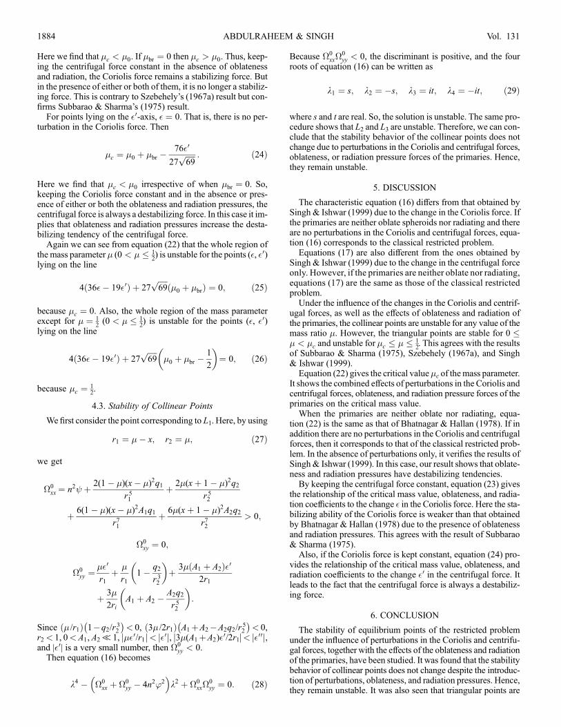
�p ¼4 36�� 19�0ð Þ

27ffiffiffiffiffi69

p :

Clearly, �c represents the combined effects of perturbations, ra-diation, and oblateness on the critical mass value of the restrictedproblem.However, in the absence of perturbations, radiation pres-sure, and oblateness of the primaries, the critical mass value �cbecomes�0, which corresponds to the classical restricted problem.

But in the absence of perturbations only (i.e., �p ¼ 0) in equa-tions (22), �c reduces to the critical mass value of the restrictedproblem with oblate spheroid and radiating primaries. This con-firms the result of Singh & Ishwar (1999). In this case �c < �0,which implies that the range of stability decreases. When theprimaries are nonradiating, nonoblate spheroids (i.e., �br ¼ 0),the critical mass value verifies the results of Bhatnagar & Hallan(1978). In this case �c > �0, which implies that the range of sta-bility increases. Here we conclude that in the absence of pertur-bations in the Coriolis and centrifugal forces, the oblateness andradiation pressures of the primaries have a destabilizing tendency.

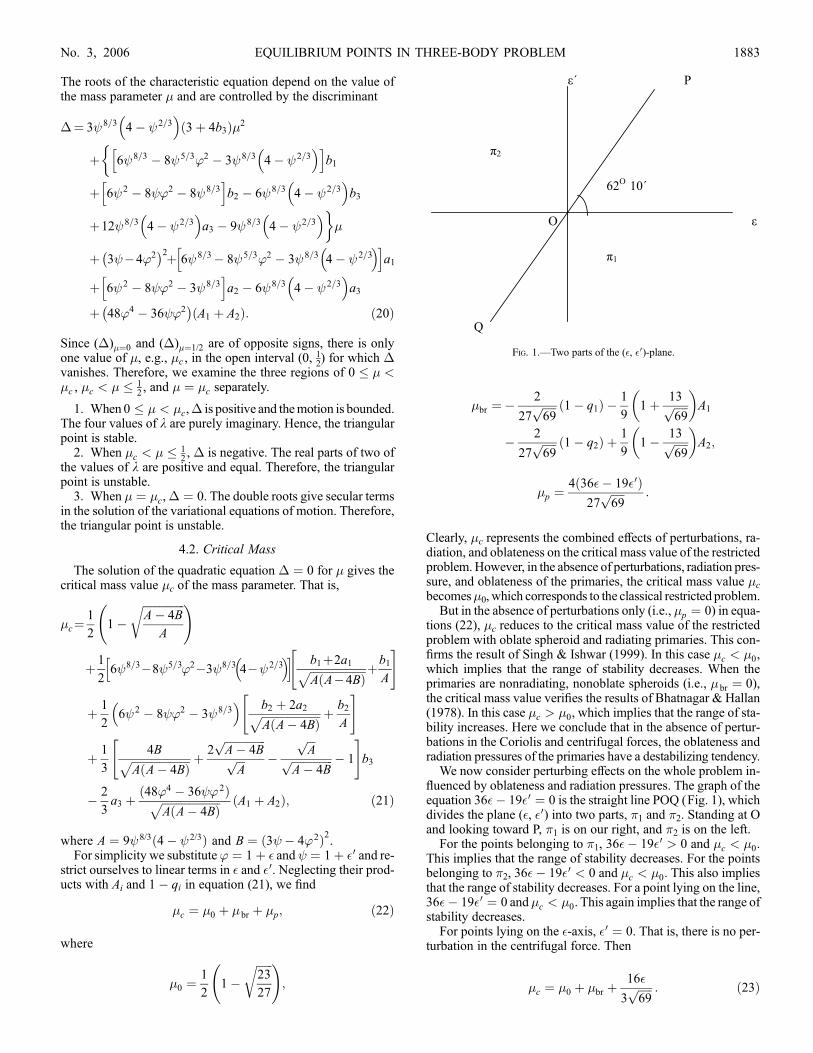
We now consider perturbing effects on the whole problem in-fluenced by oblateness and radiation pressures. The graph of theequation 36�� 19�0 ¼ 0 is the straight line POQ (Fig. 1), whichdivides the plane (�, �0) into two parts, �1 and �2. Standing at Oand looking toward P, �1 is on our right, and �2 is on the left.

For the points belonging to �1, 36�� 19�0 > 0 and �c < �0.This implies that the range of stability decreases. For the pointsbelonging to �2, 36�� 19�0 < 0 and �c < �0. This also impliesthat the range of stability decreases. For a point lying on the line,36�� 19�0 ¼ 0 and�c < �0. This again implies that the range ofstability decreases.

For points lying on the �-axis, �0 ¼ 0. That is, there is no per-turbation in the centrifugal force. Then

�c ¼ �0 þ �br þ16�

3ffiffiffiffiffi69

p : ð23Þ

Fig. 1.—Two parts of the (�, �0)-plane.

EQUILIBRIUM POINTS IN THREE-BODY PROBLEM 1883No. 3, 2006

Here we find that �c < �0. If �br ¼ 0 then �c > �0. Thus, keep-ing the centrifugal force constant in the absence of oblatenessand radiation, the Coriolis force remains a stabilizing force. Butin the presence of either or both of them, it is no longer a stabiliz-ing force. This is contrary to Szebehely’s (1967a) result but con-firms Subbarao & Sharma’s (1975) result.

For points lying on the �0-axis, � ¼ 0. That is, there is no per-turbation in the Coriolis force. Then

�c ¼ �0 þ �br �76�0

27ffiffiffiffiffi69

p : ð24Þ

Here we find that �c < �0 irrespective of when �br ¼ 0. So,keeping the Coriolis force constant and in the absence or pres-ence of either or both the oblateness and radiation pressures, thecentrifugal force is always a destabilizing force. In this case it im-plies that oblateness and radiation pressures increase the desta-bilizing tendency of the centrifugal force.

Again we can see from equation (22) that the whole region ofthe mass parameter � (0 < � � 1

2) is unstable for the points (�, �0)

lying on the line

4 36�� 19�0ð Þ þ 27ffiffiffiffiffi69

p�0 þ �brð Þ ¼ 0; ð25Þ

because �c ¼ 0. Also, the whole region of the mass parameterexcept for � ¼ 1

2(0 < � � 1

2) is unstable for the points (�, �0)

lying on the line

4 36�� 19�0ð Þ þ 27ffiffiffiffiffi69

p�0 þ �br �

1

2

� �¼ 0; ð26Þ

because �c ¼ 12.

4.3. Stability of Collinear Points

Wefirst consider the point corresponding to L1. Here, by using

r1 ¼ �� x; r2 ¼ �; ð27Þ

we get

�0xx ¼ n2 þ 2(1� �)(x� �)2q1

r 51þ 2�(xþ 1� �)2q2

r 52

þ 6(1� �)(x� �)2A1q1

r71þ 6�(xþ 1� �)2A2q2

r72> 0;

�0xy ¼ 0;

�0yy ¼

��0

r1þ �

r11� q2

r 32

� �þ 3� A1 þ A2ð Þ�0

2r1

þ 3�

2riA1 þ A2 �

A2q2

r 52

� �:

Since � /r1ð Þ 1�q2/r32

� �< 0, 3� /2r1ð Þ A1þA2�A2q2/r

52

� �< 0,

r2< 1, 0<A1, A2T1, ��0/r1j j< �0j j, 3�(A1þA2)�0/2r1j j< �00j j,

and |�0| is a very small number, then �0yy < 0.

Then equation (16) becomes

k4 � �0xx þ �0

yy � 4n2’2�

k2 þ �0xx�

0yy ¼ 0: ð28Þ

Because �0xx�

0yy < 0, the discriminant is positive, and the four

roots of equation (16) can be written as

k1 ¼ s; k2 ¼ �s; k3 ¼ it; k4 ¼ �it; ð29Þ

where s and t are real. So, the solution is unstable. The same pro-cedure shows that L2 and L3 are unstable. Therefore, we can con-clude that the stability behavior of the collinear points does notchange due to perturbations in the Coriolis and centrifugal forces,oblateness, or radiation pressure forces of the primaries. Hence,they remain unstable.

5. DISCUSSION

The characteristic equation (16) differs from that obtained bySingh & Ishwar (1999) due to the change in the Coriolis force. Ifthe primaries are neither oblate spheroids nor radiating and thereare no perturbations in the Coriolis and centrifugal forces, equa-tion (16) corresponds to the classical restricted problem.Equations (17) are also different from the ones obtained by

Singh & Ishwar (1999) due to the change in the centrifugal forceonly. However, if the primaries are neither oblate nor radiating,equations (17) are the same as those of the classical restrictedproblem.Under the influence of the changes in the Coriolis and centrif-

ugal forces, as well as the effects of oblateness and radiation ofthe primaries, the collinear points are unstable for any value of themass ratio �. However, the triangular points are stable for 0 �� < �c and unstable for �c � � � 1

2. This agrees with the results

of Subbarao & Sharma (1975), Szebehely (1967a), and Singh& Ishwar (1999).Equation (22) gives the critical value�c of themass parameter.

It shows the combined effects of perturbations in the Coriolis andcentrifugal forces, oblateness, and radiation pressure forces of theprimaries on the critical mass value.When the primaries are neither oblate nor radiating, equa-

tion (22) is the same as that of Bhatnagar & Hallan (1978). If inaddition there are no perturbations in the Coriolis and centrifugalforces, then it corresponds to that of the classical restricted prob-lem. In the absence of perturbations only, it verifies the results ofSingh& Ishwar (1999). In this case, our result shows that oblate-ness and radiation pressures have destabilizing tendencies.By keeping the centrifugal force constant, equation (23) gives

the relationship of the critical mass value, oblateness, and radia-tion coefficients to the change � in the Coriolis force. Here the sta-bilizing ability of the Coriolis force is weaker than that obtainedby Bhatnagar & Hallan (1978) due to the presence of oblatenessand radiation pressures. This agrees with the result of Subbarao& Sharma (1975).Also, if the Coriolis force is kept constant, equation (24) pro-

vides the relationship of the critical mass value, oblateness, andradiation coefficients to the change �0 in the centrifugal force. Itleads to the fact that the centrifugal force is always a destabiliz-ing force.

6. CONCLUSION

The stability of equilibrium points of the restricted problemunder the influence of perturbations in the Coriolis and centrifu-gal forces, together with the effects of the oblateness and radiationof the primaries, have been studied. It was found that the stabilitybehavior of collinear points does not change despite the introduc-tion of perturbations, oblateness, and radiation pressures. Hence,they remain unstable. It was also seen that triangular points are

ABDULRAHEEM & SINGH1884 Vol. 131

stable for 0 � � < �c and unstable for �c � � � 12, where �c is

the critical mass value, which depends on the joint effects of theparameters.

It was further seen that oblateness and radiation coefficientshave destabilizing tendencies, and in the presence of either orboth of them, the stabilizing behavior of the Coriolis force be-comes weak, while the destabilizing tendency of the centrifugal

force increases. The overall effect is that the range of stability ofthe triangular points decreases.

The authors are extremely grateful to D. Singh, the head of theDepartment of Mathematics at Ahmadu Bello University, Zaria,for his encouragement.

REFERENCES

Bhatnagar, K. B., & Hallan, P. P. 1978, Celest. Mech., 18, 105———. 2002, Celest. Mech. Dyn. Astron., 84, 1Kunitsyn, A. L. 2000, J. Appl. Mech., 64, 757———. 2001, J. Appl. Mech., 65, 703McCuskey, S. W. 1963, Introduction to Celestial Mechanics (New York:Addison-Wesley)

Sharma, R. K. 1982, in Sun and Planetary System, ed. W. Fricke & G. Teleki(Dordrecht: Reidel), 435

Simmons, J. F. L.,McDonald, A. J. C., &Brown, J. C. 1985,Celest.Mech., 35, 145Singh, J., & Ishwar, B. 1999, Bull. Astron. Soc. India, 27, 415Subbarao, P. V., & Sharma, R. K. 1975, A&A, 43, 381Szebehely, V. 1967a, AJ, 72, 7Szebehely, V. G. 1967b, Theory of Orbits: The Restricted Problem of ThreeBodies (New York: Academic)

Wintner, A. 1941, TheAnalytical Foundations of CelestialMechanics (Princeton:Princeton Univ. Press)

EQUILIBRIUM POINTS IN THREE-BODY PROBLEM 1885No. 3, 2006