Embed Size (px)
Citation preview
7/28/2019 Combined Structures 2009-10
http://slidepdf.com/reader/full/combined-structures-2009-10 1/106
Structural Analysis IV
Virtual Work – Combined Structures
4th Year
Structural Engineering
2009/10
Dr. Colin Caprani
Dr. C. Caprani1
7/28/2019 Combined Structures 2009-10
http://slidepdf.com/reader/full/combined-structures-2009-10 2/106
Structural Analysis IV
Contents
1. Introduction .........................................................................................................4
1.1 Purpose ............................................................................................................ 4
2. Virtual Work Development ................................................................................ 5
2.1 The Principle of Virtual Work......................................................................... 5
2.2 Virtual Work for Deflections........................................................................... 9
2.3 Virtual Work for Indeterminate Structures....................................................10
2.4 Virtual Work for Combined Structures .........................................................12
3. Examples ............................................................................................................14
3.1 Example 1 ...................................................................................................... 14
3.2 Example 2 ...................................................................................................... 15
3.3 Example 3 ...................................................................................................... 16
3.4 Example 4 ...................................................................................................... 22
3.5 Further Examples........................................................................................... 29
4. Exercises ............................................................................................................. 30
4.1 Problems ........................................................................................................ 30
4.2 Past Exam Questions ..................................................................................... 32
5. Appendix – Trigonometric Integrals ............................................................... 36
5.1 Useful Identities............................................................................................. 36
5.2 Basic Results.................................................................................................. 37
5.3 Common Integrals ......................................................................................... 38
6. Appendix – Volume Integrals........................................................................... 45
7. Ring Beam Examples (Advanced) ...................................................................46
7.1 Example 1 ...................................................................................................... 46
7.2 Example 2 ...................................................................................................... 51
7.3 Example 3 ...................................................................................................... 58
7.4 Example 4 ...................................................................................................... 66
7.5 Example 5 ...................................................................................................... 75
Dr. C. Caprani2
7/28/2019 Combined Structures 2009-10
http://slidepdf.com/reader/full/combined-structures-2009-10 3/106
Structural Analysis IV
7.6 Review of Examples 1 – 5 .............................................................................96
Dr. C. Caprani3
7/28/2019 Combined Structures 2009-10
http://slidepdf.com/reader/full/combined-structures-2009-10 4/106
Structural Analysis IV
1. Introduction
1.1 Purpose
Previously we only used virtual work to analyse structures whose members primarily
behaved in flexure or in axial forces. Many real structures are comprised of a mixture
of such members. Cable-stay and suspension bridges area good examples: the deck-
level carries load primarily through bending whilst the cable and pylon elements
carry load through axial forces mainly. A simple example is:
Our knowledge of virtual work to-date is sufficient to analyse such structures.
Dr. C. Caprani4
7/28/2019 Combined Structures 2009-10
http://slidepdf.com/reader/full/combined-structures-2009-10 5/106
Structural Analysis IV
2. Virtual Work Development
2.1 The Princip le of Virtual Work
This states that:
A body is in equilibrium if, and only if, the virtual work of all forces acting on
the body is zero.
In this context, the word ‘virtual’ means ‘having the effect of, but not the actual form
of, what is specified’.
There are two ways to define virtual work, as follows.
1. Virtual Displacement:
Virtual work is the work done by the actual forces acting on the body moving
through a virtual displacement.
2. Virtual Force:
Virtual work is the work done by a virtual force acting on the body moving
through the actual displacements.
Virtual Displacements
A virtual displacement is a displacement that is only imagined to occur:
• virtual displacements must be small enough such that the force directions are
maintained.
• virtual displacements within a body must be geometrically compatible with
the original structure. That is, geometrical constraints (i.e. supports) and
member continuity must be maintained.
Dr. C. Caprani5
7/28/2019 Combined Structures 2009-10
http://slidepdf.com/reader/full/combined-structures-2009-10 6/106
Structural Analysis IV
Virtual Forces
A virtual force is a force imagined to be applied and is then moved through the actual
deformations of the body, thus causing virtual work.
Virtual forces must form an equilibrium set of their own.
Internal and External Virtual Work
When a structures deforms, work is done both by the applied loads moving through a
displacement, as well as by the increase in strain energy in the structure. Thus whenvirtual displacements or forces are causing virtual work, we have:
0
0 I E
E I
W
W W
W W
δ
δ δ
δ δ
=
− =
=
where
• Virtual work is denoted W δ and is zero for a body in equilibrium;
• External virtual work is E
W δ , and;
• Internal virtual work is I
W δ .
And so the external virtual work must equal the internal virtual work. It is in thisform that the Principle of Virtual Work finds most use.
Dr. C. Caprani6
7/28/2019 Combined Structures 2009-10
http://slidepdf.com/reader/full/combined-structures-2009-10 7/106
Structural Analysis IV
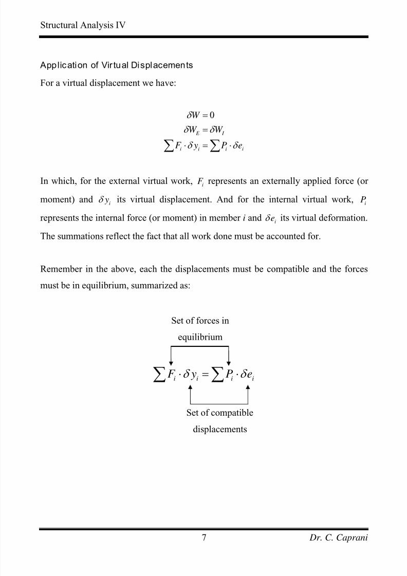
Application of Vir tual Displacements
For a virtual displacement we have:
0
E I
i i i
W
W W
iF y P e
δ
δ δ
δ δ
=
=
⋅ = ⋅∑ ∑
In which, for the external virtual work, represents an externally applied force (or
moment) and
iF
i yδ its virtual displacement. And for the internal virtual work, iP
represents the internal force (or moment) in member i and ieδ its virtual deformation.
The summations reflect the fact that all work done must be accounted for.
Remember in the above, each the displacements must be compatible and the forces
must be in equilibrium, summarized as:
Set of forces in
equilibrium
i i i iF y P eδ δ ⋅ = ⋅∑ ∑
Set of compatible
displacements
Dr. C. Caprani7
7/28/2019 Combined Structures 2009-10
http://slidepdf.com/reader/full/combined-structures-2009-10 8/106
Structural Analysis IV
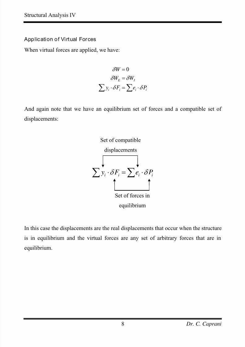
Application of Virtual Forces
When virtual forces are applied, we have:
0
E I
i i i
W
W W
y F e iP
δ
δ δ
δ δ
=
=
⋅ = ⋅∑ ∑
And again note that we have an equilibrium set of forces and a compatible set of
displacements:
Set of compatible
displacements
i i i i y F e Pδ δ ⋅ = ⋅∑ ∑
Set of forces in
equilibrium
In this case the displacements are the real displacements that occur when the structure
is in equilibrium and the virtual forces are any set of arbitrary forces that are in
equilibrium.
Dr. C. Caprani8
7/28/2019 Combined Structures 2009-10
http://slidepdf.com/reader/full/combined-structures-2009-10 9/106
Structural Analysis IV
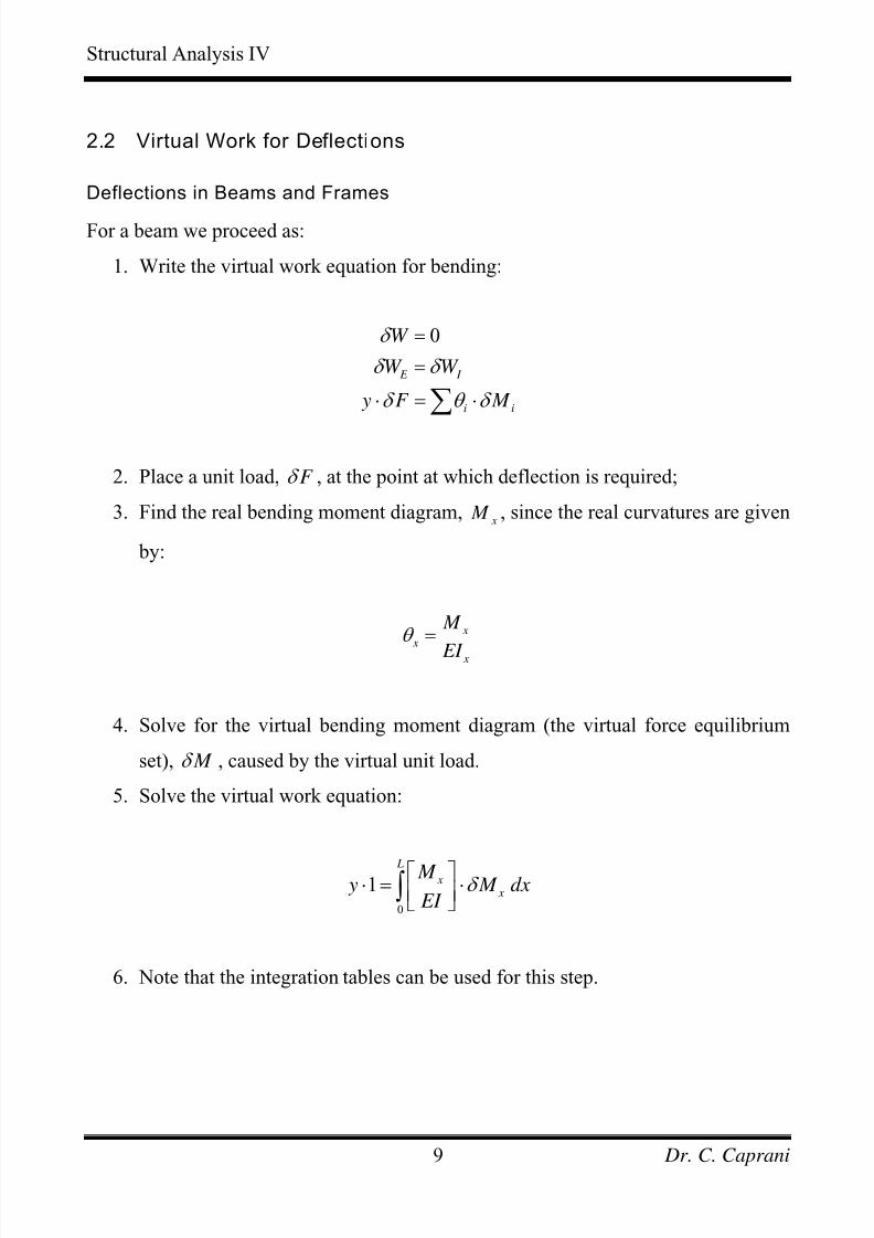
2.2 Virtual Work for Deflections
Deflections in Beams and Frames
For a beam we proceed as:
1. Write the virtual work equation for bending:
0
E I
i i
W
W W
y F M
δ
δ δ
δ θ δ
=
=
⋅ = ⋅∑
2. Place a unit load, F δ , at the point at which deflection is required;
3. Find the real bending moment diagram, x
M , since the real curvatures are given
by:
x x
x
M
EI
θ =
4. Solve for the virtual bending moment diagram (the virtual force equilibrium
set), M δ , caused by the virtual unit load.
5. Solve the virtual work equation:
0
1 L
x x
M y M EI
δ ⎡ ⎤⋅ = ⋅⎢ ⎥⎣ ⎦∫ dx
6. Note that the integration tables can be used for this step.
Dr. C. Caprani9
7/28/2019 Combined Structures 2009-10
http://slidepdf.com/reader/full/combined-structures-2009-10 10/106
Structural Analysis IV
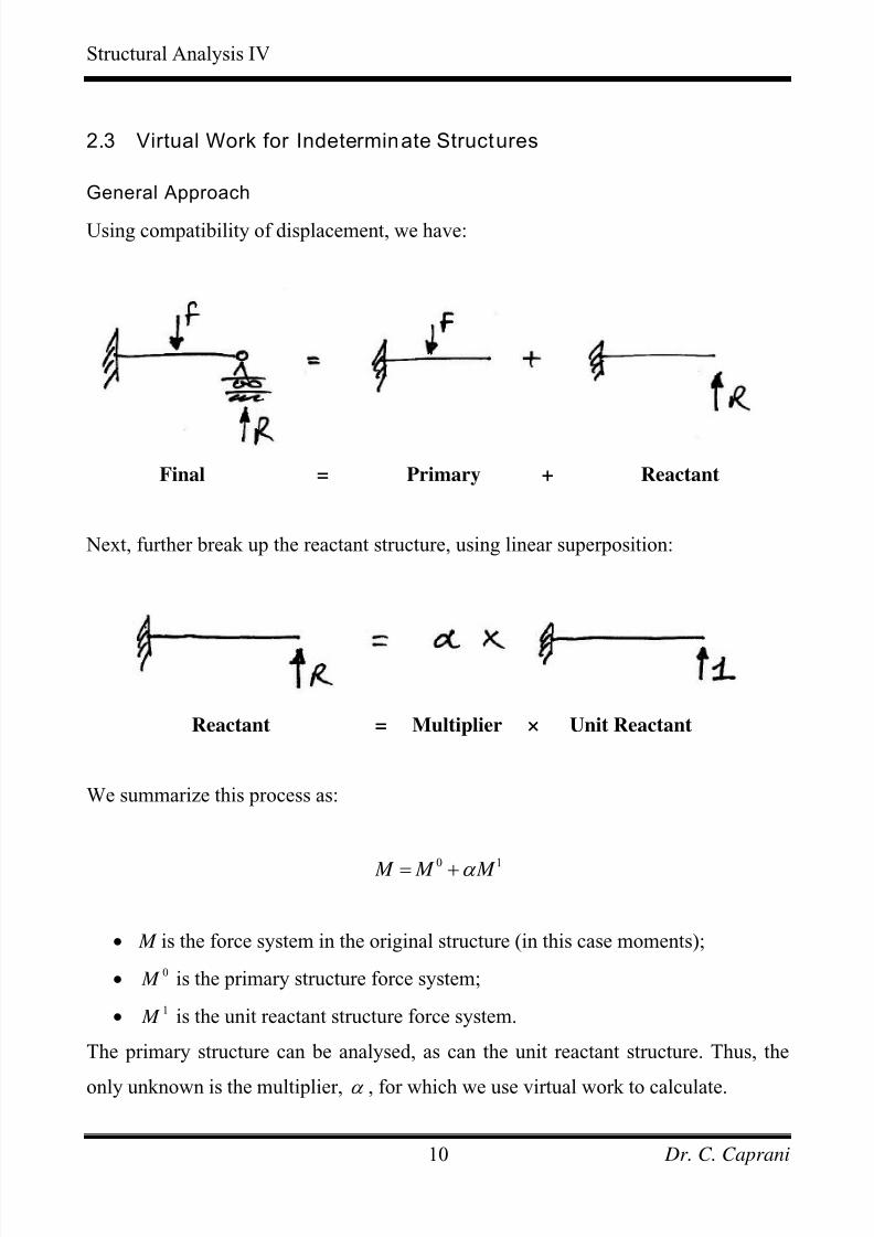
2.3 Virtual Work for Indeterminate Structures
General Approach
Using compatibility of displacement, we have:
Final = Primary + Reactant
Next, further break up the reactant structure, using linear superposition:
Reactant = Multiplier × Unit Reactant
We summarize this process as:
0 1 M M M α = +
• M is the force system in the original structure (in this case moments);
• 0 M is the primary structure force system;
• 1 M is the unit reactant structure force system.
The primary structure can be analysed, as can the unit reactant structure. Thus, the
only unknown is the multiplier, α , for which we use virtual work to calculate.
Dr. C. Caprani10
7/28/2019 Combined Structures 2009-10
http://slidepdf.com/reader/full/combined-structures-2009-10 11/106
Structural Analysis IV
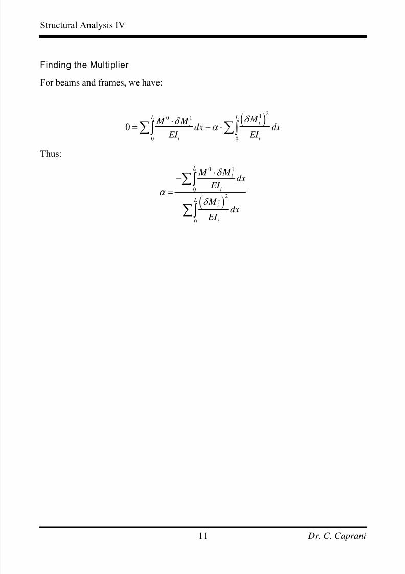
Finding the Multiplier
For beams and frames, we have:
( )2
10 1
0 0
0
L Lii
i i
M M M dx dx
EI EI
δ δ α
⋅= + ⋅∑ ∑∫ ∫
Thus:
( )
0 1
02
1
0
L
i
i
L i
i
M M dx
EI
M dx
EI
δ
α
δ
⋅−
=∑∫
∑∫
Dr. C. Caprani11
7/28/2019 Combined Structures 2009-10
http://slidepdf.com/reader/full/combined-structures-2009-10 12/106
Structural Analysis IV
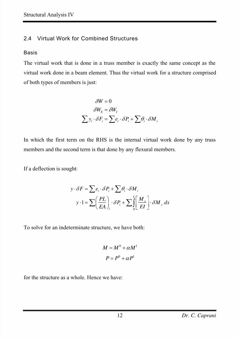
2.4 Virtual Work for Combined Structures
Basis
The virtual work that is done in a truss member is exactly the same concept as the
virtual work done in a beam element. Thus the virtual work for a structure comprised
of both types of members is just:
0
E I
i i i i i
W
W W
y F e P M i
δ
δ δ
δ δ θ δ
=
=
⋅ = ⋅ + ⋅∑ ∑ ∑
In which the first term on the RHS is the internal virtual work done by any truss
members and the second term is that done by any flexural members.
If a deflection is sought:
0
1
i i i i
L
xi x
i
y F e P M
PL M y P
EA EI
δ δ θ δ
δ δ
⋅ = ⋅ + ⋅
⎛ ⎞ ⎡ ⎤⋅ = ⋅ + ⋅⎜ ⎟ ⎢ ⎥⎝ ⎠ ⎣ ⎦
∑ ∑
∑ ∑∫ M dx
To solve for an indeterminate structure, we have both:
0 1 M M M α = +
0 1P P Pα = +
for the structure as a whole. Hence we have:
Dr. C. Caprani12
7/28/2019 Combined Structures 2009-10
http://slidepdf.com/reader/full/combined-structures-2009-10 13/106
Structural Analysis IV
( ) ( )
( )
1
0
0 1 0 1
1
0
210 1 0 1
1 1
0
0
0 1
0
0
E I
i i i i i i
L x
i x
i
L x x
i x
i
L x x x
i i
i i
W
W W
y F e P M
PL M P M dx
EA EI
P P L M M P M dx
EA EI
M P L P L M M P P dx
EA EA EI
δ
δ δ
δ δ θ δ
δ δ
α δ α δ δ
δ δ δ δ α δ α
=
=
⋅ = ⋅ + ⋅
⎛ ⎞ ⎡ ⎤⋅ = ⋅ + ⋅⎜ ⎟ ⎢ ⎥⎝ ⎠ ⎣ ⎦
⎛ ⎞ ⎡ ⎤+ ⋅ +⎜ ⎟= ⋅ + ⋅⎢ ⎥⎜ ⎟ ⎢ ⎥⎝ ⎠ ⎣ ⎦
⎛ ⎞ ⎛ ⎞ ⋅= ⋅ + ⋅ ⋅ + + ⋅⎜ ⎟ ⎜ ⎟
⎝ ⎠ ⎝ ⎠
∑ ∑ ∑
∑ ∑∫
∑ ∑∫
∑ ∑ ∑∫0
L
dx EI
∑∫
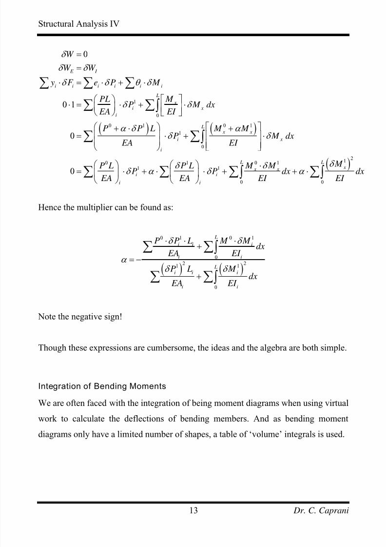
Hence the multiplier can be found as:
( ) ( )
0 1 0 1
02 2
1 1
0
L
i i i
i i
Li i i
i i
P P L M M dx
EA EI
P L M dx
EA EI
δ δ
α δ δ
⋅ ⋅ ⋅+
= −
+
∑ ∑∫
∑ ∑∫
Note the negative sign!
Though these expressions are cumbersome, the ideas and the algebra are both simple.
Integration of Bending Moments
We are often faced with the integration of being moment diagrams when using virtual
work to calculate the deflections of bending members. And as bending moment
diagrams only have a limited number of shapes, a table of ‘volume’ integrals is used.
Dr. C. Caprani13
7/28/2019 Combined Structures 2009-10
http://slidepdf.com/reader/full/combined-structures-2009-10 14/106
Structural Analysis IV
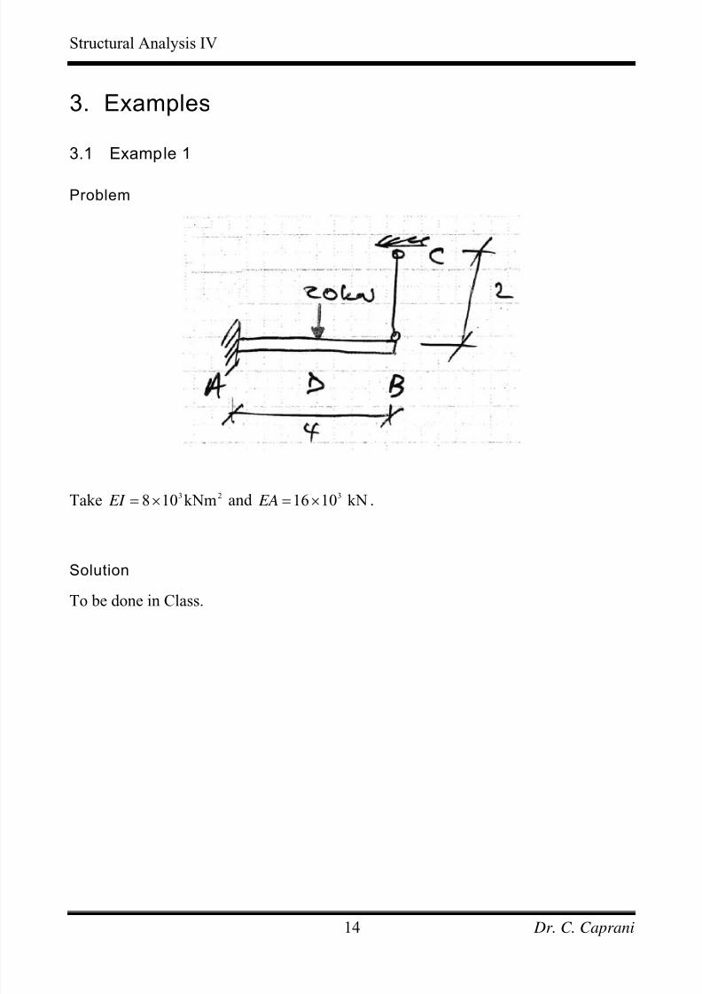
3. Examples
3.1 Example 1
Problem
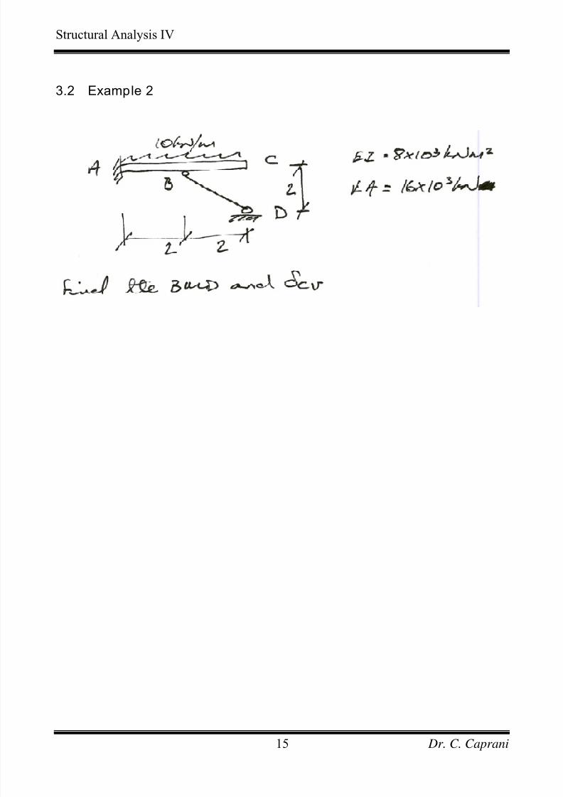
Take 38 10 kNm2 EI = × and 316 10 kN EA = × .
Solution
To be done in Class.
Dr. C. Caprani14
7/28/2019 Combined Structures 2009-10
http://slidepdf.com/reader/full/combined-structures-2009-10 15/106
Structural Analysis IV
3.2 Example 2
Dr. C. Caprani15
7/28/2019 Combined Structures 2009-10
http://slidepdf.com/reader/full/combined-structures-2009-10 16/106
Structural Analysis IV
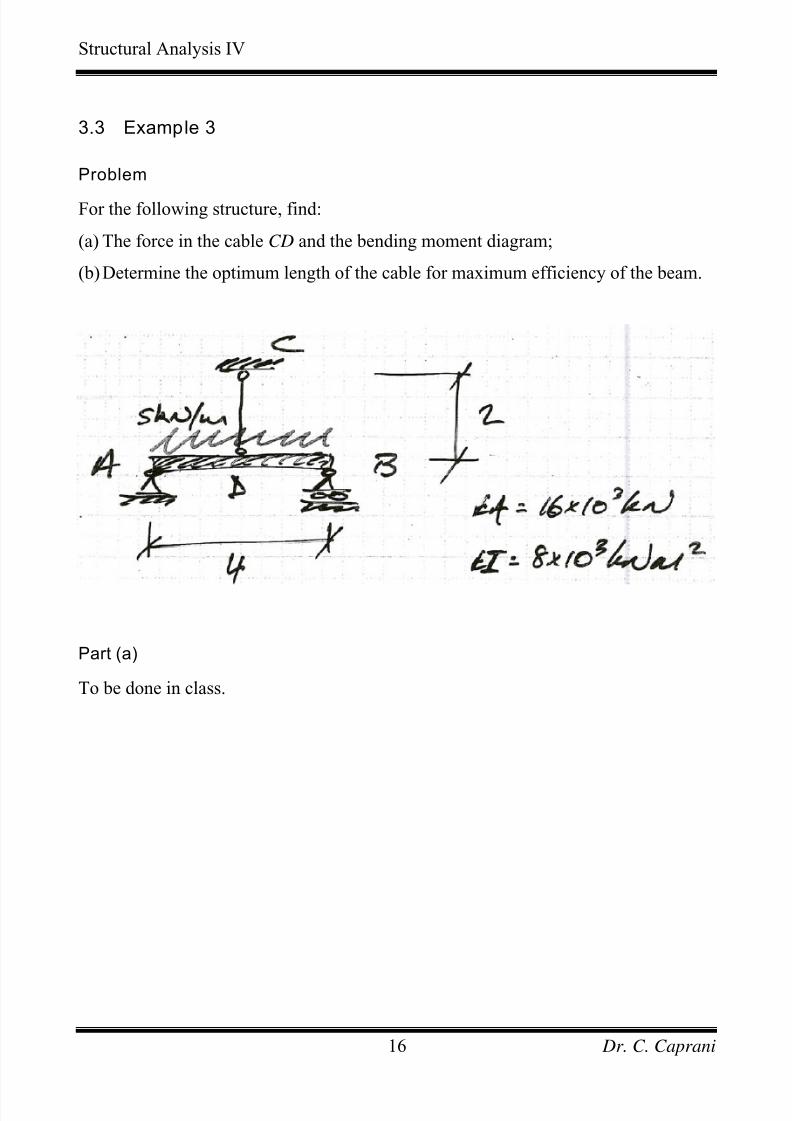
3.3 Example 3
Problem
For the following structure, find:
(a) The force in the cable CD and the bending moment diagram;
(b) Determine the optimum length of the cable for maximum efficiency of the beam.
Part (a)
To be done in class.
Dr. C. Caprani16
7/28/2019 Combined Structures 2009-10
http://slidepdf.com/reader/full/combined-structures-2009-10 17/106
Structural Analysis IV
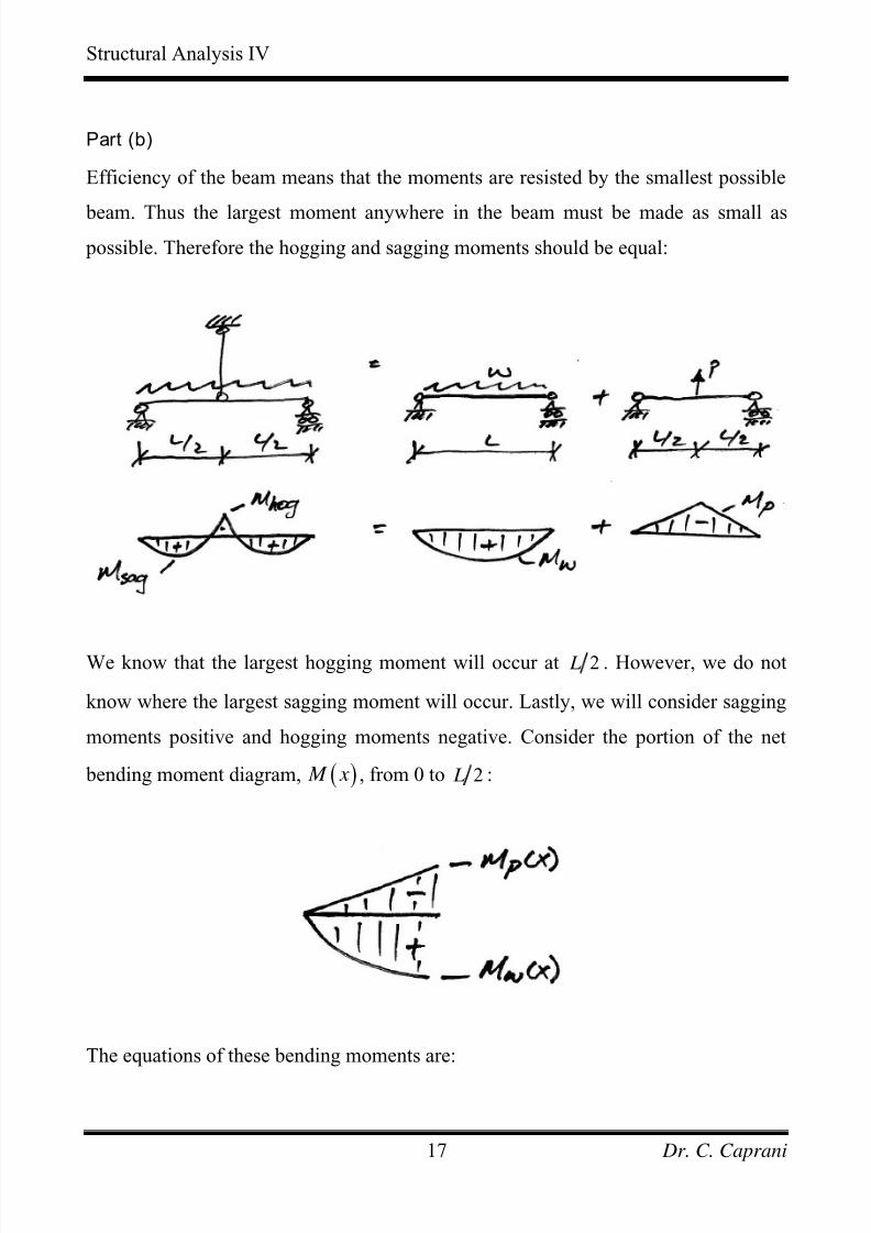
Part (b)
Efficiency of the beam means that the moments are resisted by the smallest possible
beam. Thus the largest moment anywhere in the beam must be made as small as
possible. Therefore the hogging and sagging moments should be equal:
We know that the largest hogging moment will occur at 2 L . However, we do not
know where the largest sagging moment will occur. Lastly, we will consider sagging
moments positive and hogging moments negative. Consider the portion of the net
bending moment diagram, ( ) M x , from 0 to 2 L :
The equations of these bending moments are:
Dr. C. Caprani17
7/28/2019 Combined Structures 2009-10
http://slidepdf.com/reader/full/combined-structures-2009-10 18/106
Structural Analysis IV
( )2
P
P M x x= −
( ) 2
2 2W
w wL M x x= − + x
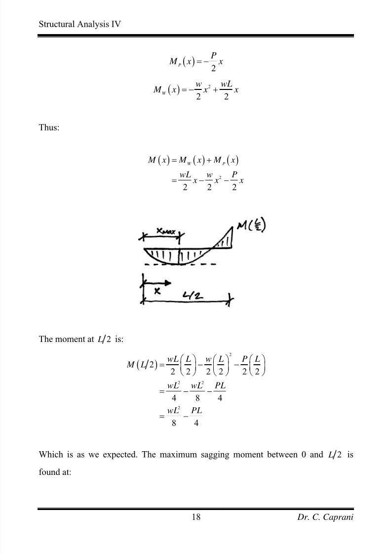
Thus:
( ) ( ) ( )
2
2 2 2
W P M x M x M x
wL w P x x x
= +
= − −
The moment at 2 L is:
( )2
2 2
2
22 2 2 2 2 2
4 8 4
8 4
wL L w L P L M L
wL wL PL
wL PL
⎛ ⎞ ⎛ ⎞ ⎛ ⎞= − −⎜ ⎟ ⎜ ⎟ ⎜ ⎟
⎝ ⎠ ⎝ ⎠ ⎝ ⎠
= − −
= −
Which is as we expected. The maximum sagging moment between 0 and 2 L is
found at:
Dr. C. Caprani18
7/28/2019 Combined Structures 2009-10
http://slidepdf.com/reader/full/combined-structures-2009-10 19/106
Structural Analysis IV
( )
max
max
0
0
2 2
2 2
dM x
dx
wL Pwx
L P x
w
=
− − =
= −
Thus the maximum sagging moment has a value:
( )
2
max
2 2 2
2 2
2 2 2 2 2 2 2 2 2
2
4 4 2 4 4 4 4 4
8 4 8
wL L P w L P P L P M x
w w
wL PL w L PL P PL P
w w
wL PL P
w
⎛ ⎞ ⎛ ⎞ ⎛ ⎞= − − − − −
⎜ ⎟ ⎜ ⎟ ⎜ ⎟⎝ ⎠ ⎝ ⎠ ⎝ ⎠⎛ ⎞
= − − − + − +⎜ ⎟⎝ ⎠
= − +
2
w
w
Since we have assigned a sign convention, the sum of the hogging and sagging
moments should be zero, if we are to achieve the optimum BMD. Thus:
( ) ( )max
2 2 2
2 2
2
2
2 0
08 4 8 8 4
0
4 2 81
08 2 4
M x M L
wL PL P wL PL
w
wL PL P
w L wL
P Pw
+ =
⎡ ⎤ ⎡− + + − =⎢ ⎥ ⎢
⎣ ⎦ ⎣
⎤⎥⎦
− + =
⎛ ⎞⎛ ⎞ ⎛ ⎞+ − + =⎜ ⎟ ⎜ ⎟ ⎜ ⎟
⎝ ⎠ ⎝ ⎠ ⎝ ⎠
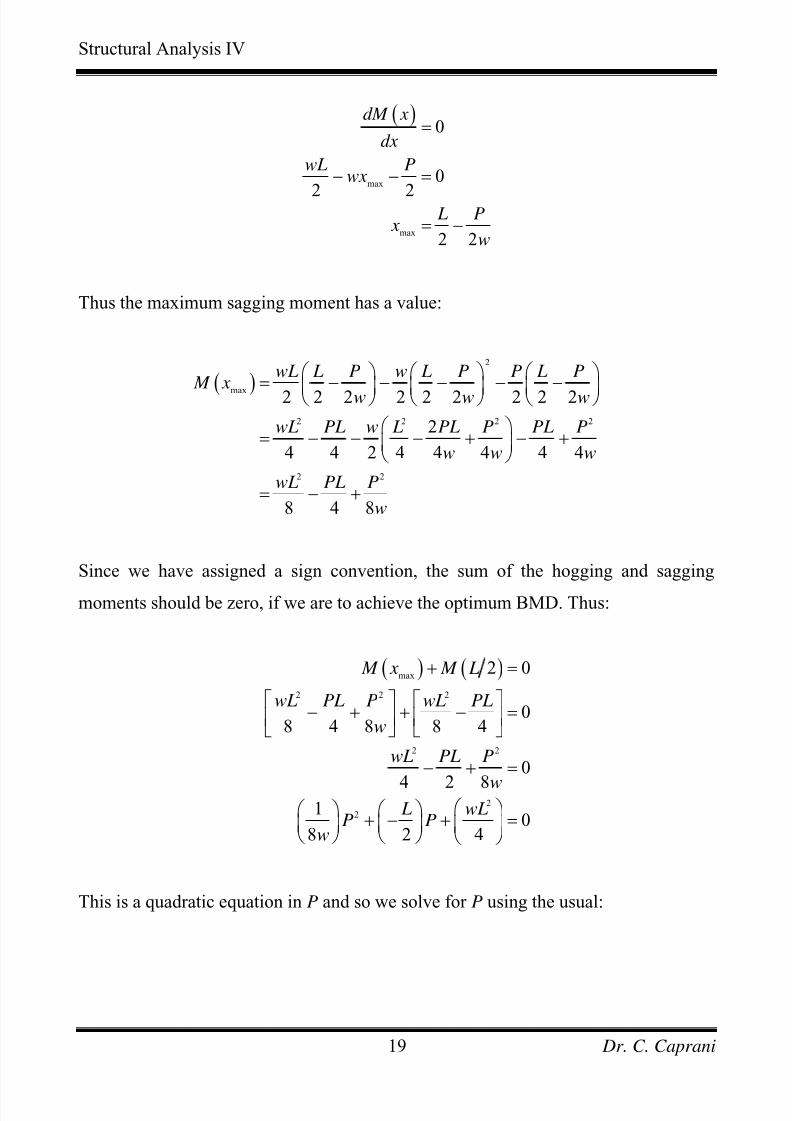
This is a quadratic equation in P and so we solve for P using the usual:
Dr. C. Caprani19
7/28/2019 Combined Structures 2009-10
http://slidepdf.com/reader/full/combined-structures-2009-10 20/106
Structural Analysis IV
( )
2 2
2 4 82
88
2 2 8
2 2
L L L
P
ww L L
wL
± −=
⎛ ⎞= ±⎜ ⎟
⎝ ⎠
= ±
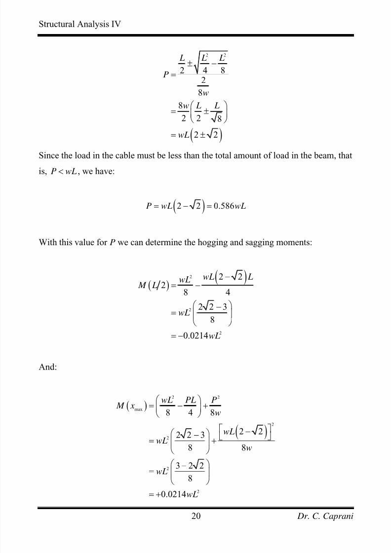
Since the load in the cable must be less than the total amount of load in the beam, that
is, , we have:P wL<
( )2 2 0.586P wL wL= − =
With this value for P we can determine the hogging and sagging moments:
( )
( )2
2
2
2 22
8 4
2 2 3
8
0.0214
wL LwL M L
wL
wL
−= −
⎛ ⎞−= ⎜ ⎟
⎝ ⎠
= −
And:
( )
( )
2 2
max
2
2
2
2
8 4 8
2 22 2 3
8 8
3 2 2
8
0.0214
wL PL P M x
w
wLwL
w
wL
wL
⎛ ⎞= − +⎜ ⎟
⎝ ⎠
⎡ ⎤−⎛ ⎞− ⎣ ⎦= +⎜ ⎟⎝ ⎠
⎛ ⎞−= ⎜ ⎟
⎝ ⎠= +
Dr. C. Caprani20
7/28/2019 Combined Structures 2009-10
http://slidepdf.com/reader/full/combined-structures-2009-10 21/106
Structural Analysis IV
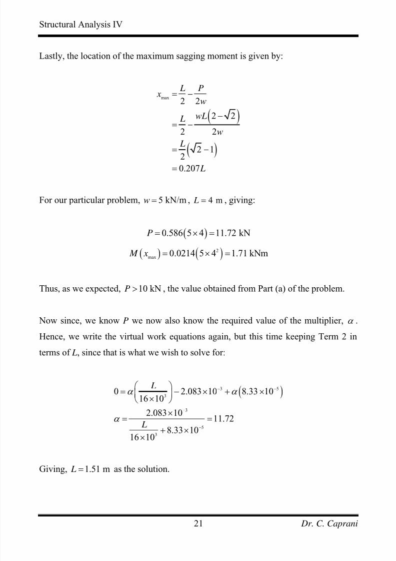
Lastly, the location of the maximum sagging moment is given by:
( )
( )
max 2 2
2 2
2 2
2 12
0.207
L P
x w
wL L
w
L
L
= −
−= −
= −
=
For our particular problem, ,5 kN/mw = 4 m L = , giving:
( )0.586 5 4 11.72 kNP = × =
( ) ( )2
max0.0214 5 4 1.71 kNm M x = × =
Thus, as we expected, , the value obtained from Part (a) of the problem.10 kNP >
Now since, we know P we now also know the required value of the multiplier, α .
Hence, we write the virtual work equations again, but this time keeping Term 2 in
terms of L, since that is what we wish to solve for:
( )3 5
3
3
5
3
0 2.083 10 8.33 1016 10
2.083 1011.72
8.33 1016 10
L
L
α α
α
− −
−
−
⎛ ⎞
= − × + ×⎜ ⎟×⎝ ⎠
×= =
+ ××
Giving, 1.51 m L = as the solution.
Dr. C. Caprani21
7/28/2019 Combined Structures 2009-10
http://slidepdf.com/reader/full/combined-structures-2009-10 22/106
Structural Analysis IV
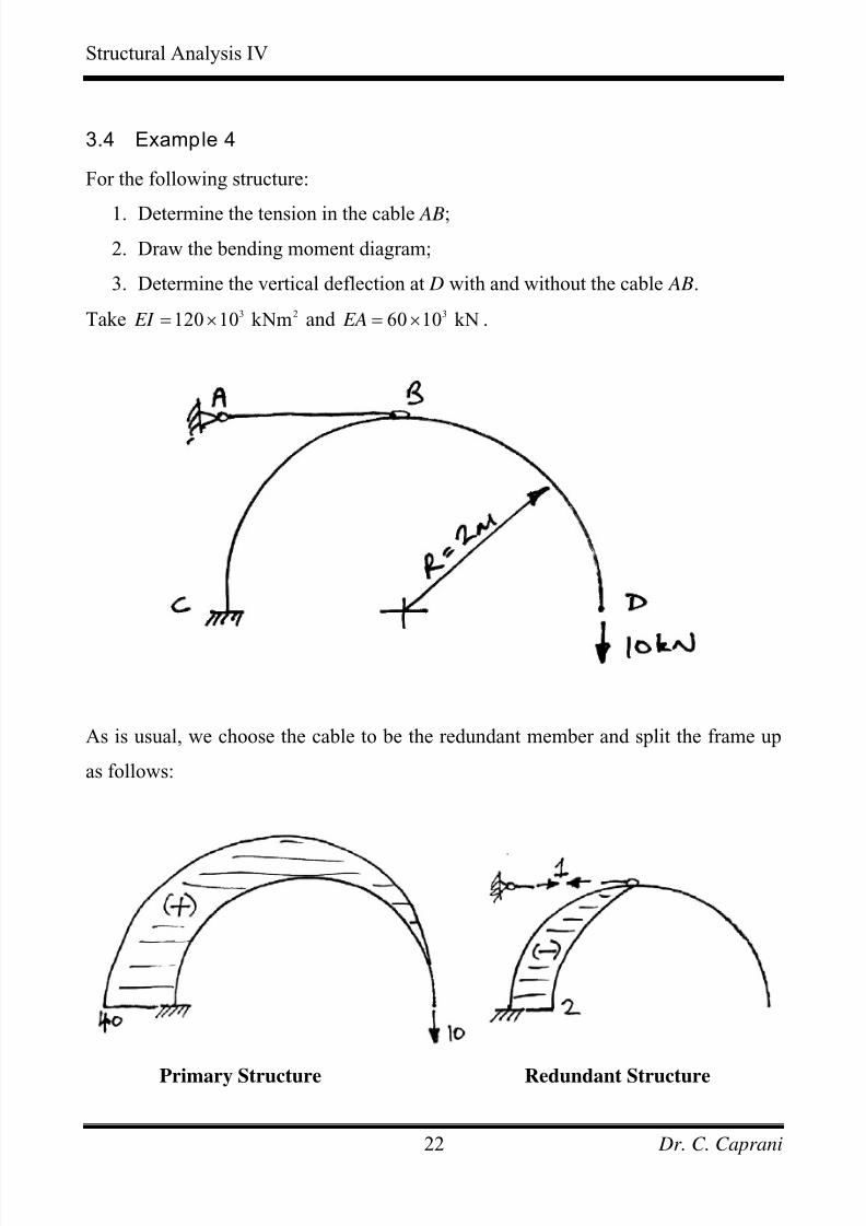
3.4 Example 4
For the following structure:
1. Determine the tension in the cable AB;
2. Draw the bending moment diagram;
3. Determine the vertical deflection at D with and without the cable AB.
Take 3 2120 10 kNm EI = × and 360 10 kN EA = × .
As is usual, we choose the cable to be the redundant member and split the frame up
as follows:
Primary Structure Redundant Structure
Dr. C. Caprani22
7/28/2019 Combined Structures 2009-10
http://slidepdf.com/reader/full/combined-structures-2009-10 23/106
Structural Analysis IV
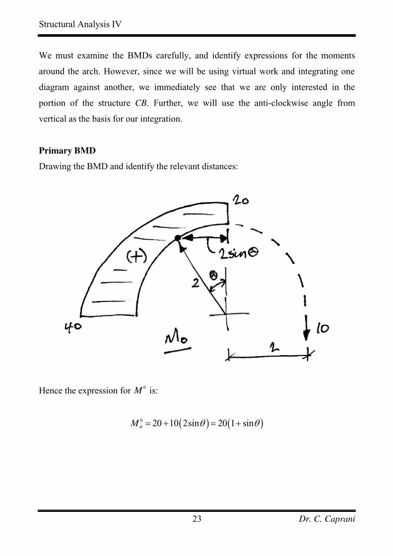
We must examine the BMDs carefully, and identify expressions for the moments
around the arch. However, since we will be using virtual work and integrating one
diagram against another, we immediately see that we are only interested in the
portion of the structure CB. Further, we will use the anti-clockwise angle from
vertical as the basis for our integration.
Primary BMD
Drawing the BMD and identify the relevant distances:
Hence the expression for 0 M is:
( ) ( )0 20 10 2sin 20 1 sin M θ
θ θ = + = +
Dr. C. Caprani23
7/28/2019 Combined Structures 2009-10
http://slidepdf.com/reader/full/combined-structures-2009-10 24/106
Structural Analysis IV
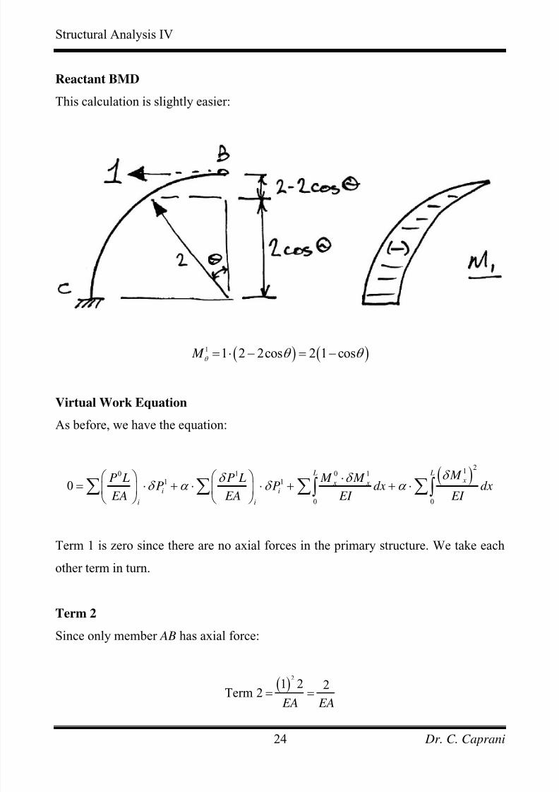
Reactant BMD
This calculation is slightly easier:
( ) ( )1 1 2 2cos 2 1 cos M θ
θ θ = ⋅ − = −
Virtual Work Equation
As before, we have the equation:
( )2
10 1 0 11 1
0 0
0 L L
x x xi i
i i
M P L P L M M P P dx
EA EA EI EI
δ δ δ δ α δ α
⎛ ⎞ ⎛ ⎞ ⋅= ⋅ + ⋅ ⋅ + + ⋅⎜ ⎟ ⎜ ⎟
⎝ ⎠ ⎝ ⎠∑ ∑ ∑ ∑∫ ∫ dx
Term 1 is zero since there are no axial forces in the primary structure. We take each
other term in turn.
Term 2
Since only member AB has axial force:
( )2
1 2 2Term 2 EA EA= =
Dr. C. Caprani24
7/28/2019 Combined Structures 2009-10
http://slidepdf.com/reader/full/combined-structures-2009-10 25/106
Structural Analysis IV
Term 3
Since we want to integrate around the member – an integrand - but only have the
moment expressed according to
ds
θ , we must change the integration limits by
substituting:
2ds R d d θ θ = ⋅ =
Hence:
( ) ( )
( )( )
( )
20 1
0 0
2
0
2
0
12 1 cos 20 1 sin 2
801 cos 1 sin
801 sin cos cos sin
L
x x M M dx d
EI EI
d EI
d EI
π
π
π
δ θ θ θ
θ θ θ
θ θ θ θ
⋅= − − +⎡ ⎤ ⎡⎣ ⎦ ⎣
= − + +
= − − + +
∑∫ ∫
∫
∫ θ
⎤⎦
To integrate this expression we refer to the appendix of integrals to get each of the
terms, which then give:
( )
20 1
00
80 1cos sin cos2
4
80 1 10 1 1 0 1 0
2 4
80 1 11 1
2 4 4
80 1
2
L
x x M M dx
EI EI
EI
EI
EI
π δ
θ θ θ θ
π
π
π
⋅ ⎡ ⎤= − + + −⎢ ⎥
⎣ ⎦⎧ ⎫
4
⎡ ⎤ ⎡ ⎤= − + + − − − − + + −⎨ ⎬⎢ ⎥ ⎢ ⎥⎣ ⎦ ⎣ ⎦⎩ ⎭
⎛ ⎞= − + + − +⎜ ⎟
⎝ ⎠
−⎛ ⎞= ⎜ ⎟
⎝ ⎠
∑∫
Dr. C. Caprani25
7/28/2019 Combined Structures 2009-10
http://slidepdf.com/reader/full/combined-structures-2009-10 26/106
Structural Analysis IV
Term 4
Proceeding similarly to Term 3, we have:
( )( ) ( )
( )
21 2
0 0
2
2
0
12 1 cos 2 1 cos 2
81 2cos cos
L x M
dx d EI EI
d EI
π
π
δ θ θ θ
θ θ θ
= − −⎡ ⎤ ⎡ ⎤⎣ ⎦ ⎣ ⎦
= − +
∑∫ ∫
∫
Again we refer to the integrals appendix, and so for Term 4 we then have:
( )( )
[ ]
21 2
2
0 0
2
0
81 2cos cos
8 12sin sin 2
2 4
8 1
2 0 02 4 4
8 3 7
4
L x M
dx d EI EI
EI
EI
EI
π
π
δ θ θ θ
θ θ θ θ
π π
π
= − +
⎡ ⎤⎛ ⎞= − + +⎜ ⎟⎢ ⎥
⎝ ⎠⎣ ⎦
0 0
⎧ ⎫⎡ ⎤⎛ ⎞
= − + + − − + +⎨ ⎬⎜ ⎟⎢ ⎥⎝ ⎠⎣ ⎦⎩ ⎭
−⎛ ⎞= ⎜ ⎟
⎝ ⎠
∑∫ ∫
Solution
Substituting the calculated values into the virtual work equation gives:
2 80 1 8 3 70 0
2 4 EA EI EI
π π α α
− −⎛ ⎞ ⎛ = + ⋅ + + ⋅⎜ ⎟ ⎜
⎝ ⎠ ⎝
⎞⎟
⎠
And so:
Dr. C. Caprani26
7/28/2019 Combined Structures 2009-10
http://slidepdf.com/reader/full/combined-structures-2009-10 27/106
Structural Analysis IV
80 1
2
2 8 3 7
4
EI
EA EI
π
α π
−⎛ ⎞− ⎜ ⎟
⎝ ⎠=−⎛ ⎞
+ ⎜ ⎟
⎝ ⎠
Simplifying:
20 20
3 7 EI
EA
π α
π
−=
− +
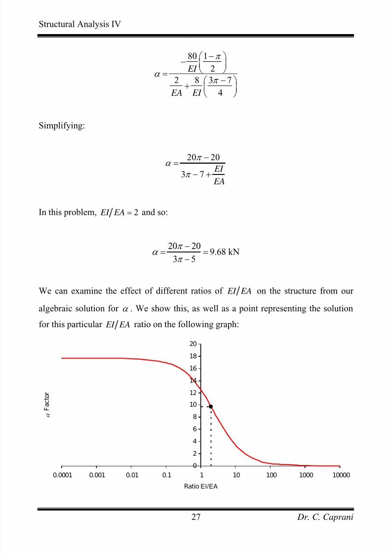
In this problem, 2 EI EA = and so:
20 209.68 kN
3 5
π α
π
−= =
−
We can examine the effect of different ratios of EI EA on the structure from our
algebraic solution for α . We show this, as well as a point representing the solution
for this particular EI EA ratio on the following graph:
0
2
4
6
8
10
12
14
16
18
20
0.0001 0.001 0.01 0.1 1 10 100 1000 10000
Ratio EI/EA
α F
a c t o r
Dr. C. Caprani27
7/28/2019 Combined Structures 2009-10
http://slidepdf.com/reader/full/combined-structures-2009-10 28/106
Structural Analysis IV
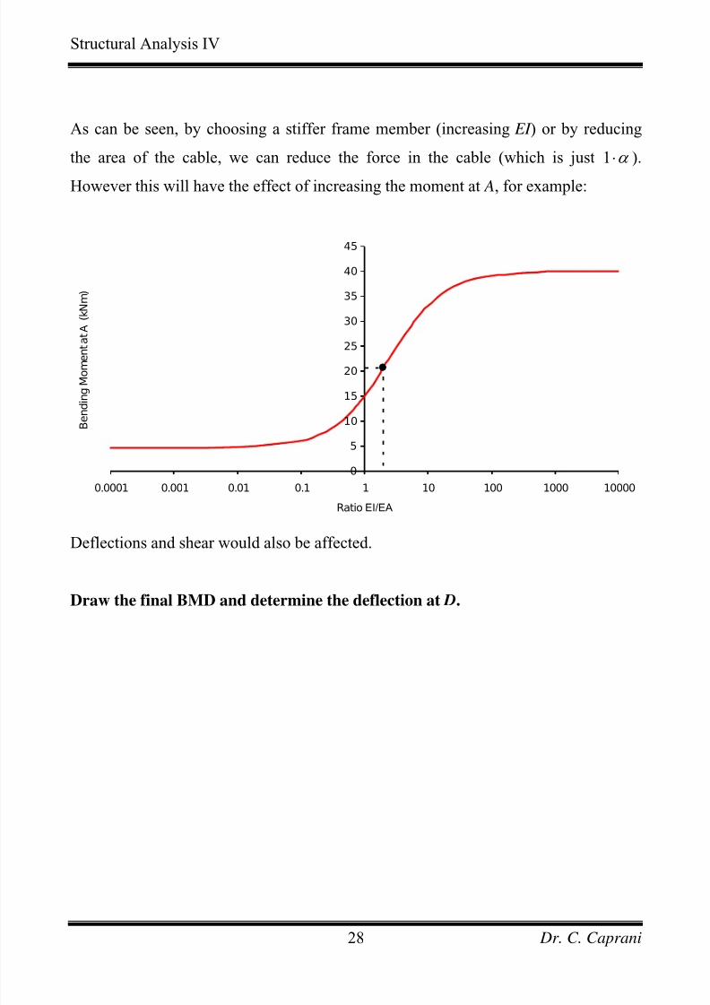
As can be seen, by choosing a stiffer frame member (increasing EI ) or by reducing
the area of the cable, we can reduce the force in the cable (which is just 1 α ⋅ ).
However this will have the effect of increasing the moment at A, for example:
0
5
10
15
20
25
30
35
40
45
0.0001 0.001 0.01 0.1 1 10 100 1000 10000
Ratio EI/EA
B e n d i n g M o m e n
t a t A ( k
N m )
Deflections and shear would also be affected.
Draw the final BMD and determine the deflection at D.
Dr. C. Caprani28
7/28/2019 Combined Structures 2009-10
http://slidepdf.com/reader/full/combined-structures-2009-10 29/106
Structural Analysis IV
3.5 Further Examples
To be done in class or given out in handout.
Dr. C. Caprani29
7/28/2019 Combined Structures 2009-10
http://slidepdf.com/reader/full/combined-structures-2009-10 30/106
Structural Analysis IV
4. Exercises
4.1 Problems
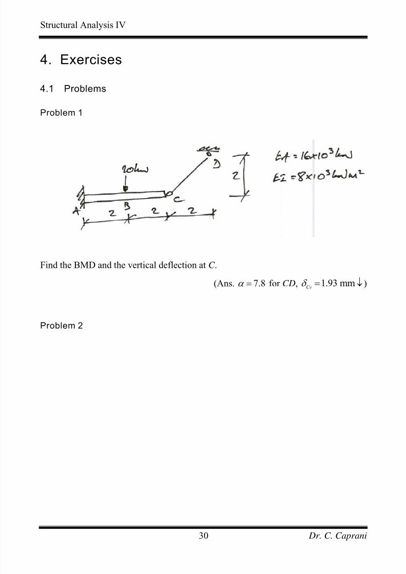
Problem 1
Find the BMD and the vertical deflection at C .
(Ans. 7.8α = for CD, )1.93 mmCv
δ = ↓
Problem 2
Dr. C. Caprani30
7/28/2019 Combined Structures 2009-10
http://slidepdf.com/reader/full/combined-structures-2009-10 31/106
Structural Analysis IV
Problem 3
Problem 4
Dr. C. Caprani31
7/28/2019 Combined Structures 2009-10
http://slidepdf.com/reader/full/combined-structures-2009-10 32/106
Structural Analysis IV
4.2 Past Exam Questions
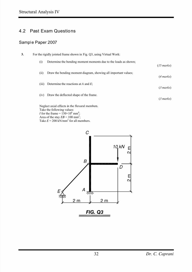
Sample Paper 2007
3. For the rigidly jointed frame shown in Fig. Q3, using Virtual Work:
(i) Determine the bending moment moments due to the loads as shown;(15 marks)
(ii) Draw the bending moment diagram, showing all important values;(4 marks)
(iii) Determine the reactions at A and E ;(3 marks)
(iv) Draw the deflected shape of the frame.(3 marks)
Neglect axial effects in the flexural members.Take the following values:
I for the frame = 150×106
mm4;
Area of the stay EB = 100 mm2;
Take E = 200 kN/mm2
for all members.
FIG. Q3
2 m
2 m
2 m
A
C
D
10 kN
B
E
2 m
Dr. C. Caprani32
7/28/2019 Combined Structures 2009-10
http://slidepdf.com/reader/full/combined-structures-2009-10 33/106
Structural Analysis IV
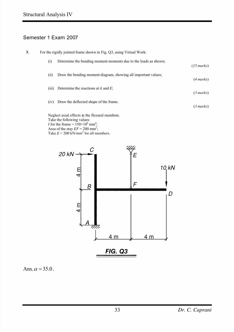
Semester 1 Exam 2007
3. For the rigidly jointed frame shown in Fig. Q3, using Virtual Work:
(i) Determine the bending moment moments due to the loads as shown;(15 marks)
(ii) Draw the bending moment diagram, showing all important values;(4 marks)
(iii) Determine the reactions at A and E ;(3 marks)
(iv) Draw the deflected shape of the frame.(3 marks)
Neglect axial effects in the flexural members.Take the following values:
I for the frame = 150×106 mm4;
Area of the stay EF = 200 mm2;
Take E = 200 kN/mm2
for all members.
FIG. Q3
4 m
4
m
4 m
A
C
D
10 kN
B
4 m
E 20 kN
F
Ans. 35.0α = .
Dr. C. Caprani33
7/28/2019 Combined Structures 2009-10
http://slidepdf.com/reader/full/combined-structures-2009-10 34/106
Structural Analysis IV
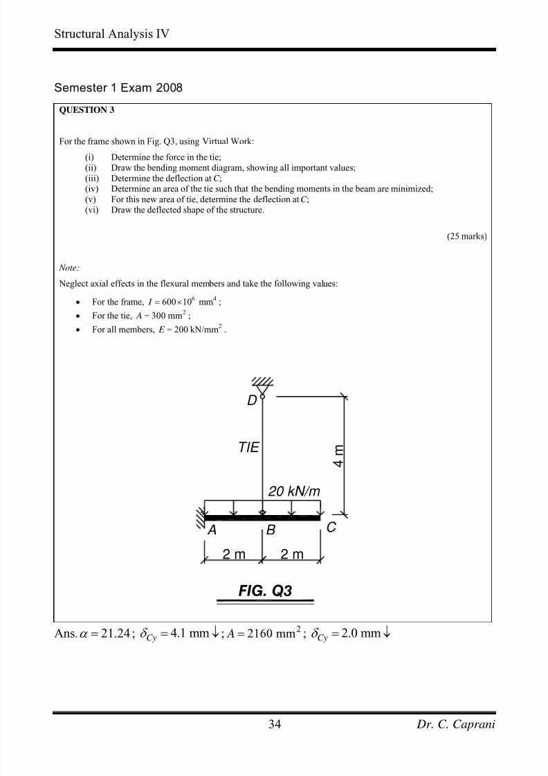
Semester 1 Exam 2008
QUESTION 3
For the frame shown in Fig. Q3, using Virtual Work:
(i) Determine the force in the tie;(ii) Draw the bending moment diagram, showing all important values;
(iii) Determine the deflection at C ;(iv) Determine an area of the tie such that the bending moments in the beam are minimized;
(v) For this new area of tie, determine the deflection at C ;(vi) Draw the deflected shape of the structure.
(25 marks)
Note: Neglect axial effects in the flexural members and take the following values:
• For the frame, ;6 4600 10 mm I = ×
• For the tie, ;2300 mm A =
• For all members, .2
200 kN/mm E =
D
4 m
A
2 m
FIG. Q3
2 m
B C
20 kN/m
TIE
Ans. 21.24α = ; ;4.1 mmCyδ = ↓ 22160 mm A = ; 2.0 mmCyδ = ↓
Dr. C. Caprani34
7/28/2019 Combined Structures 2009-10
http://slidepdf.com/reader/full/combined-structures-2009-10 35/106
Structural Analysis IV
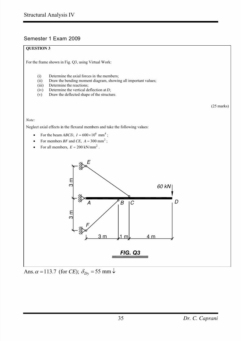
Semester 1 Exam 2009
QUESTION 3
For the frame shown in Fig. Q3, using Virtual Work:
(i) Determine the axial forces in the members;(ii) Draw the bending moment diagram, showing all important values;(iii) Determine the reactions;(iv) Determine the vertical deflection at D;(v) Draw the deflected shape of the structure.
(25 marks)
Note:
Neglect axial effects in the flexural members and take the following values:
• For the beam ABCD, ;6 4
600 10 mm I = ×
• For members BF and CE , ;2300 mm A =
• For all members, .2200 kN/mm E =
E
3 m
A
3 m
FIG. Q3
4 m
C D
F
3 m
1 m
60 kN
B
Ans. 113.7α = (for CE ); 55 mm Dyδ = ↓
Dr. C. Caprani35
7/28/2019 Combined Structures 2009-10
http://slidepdf.com/reader/full/combined-structures-2009-10 36/106
Structural Analysis IV
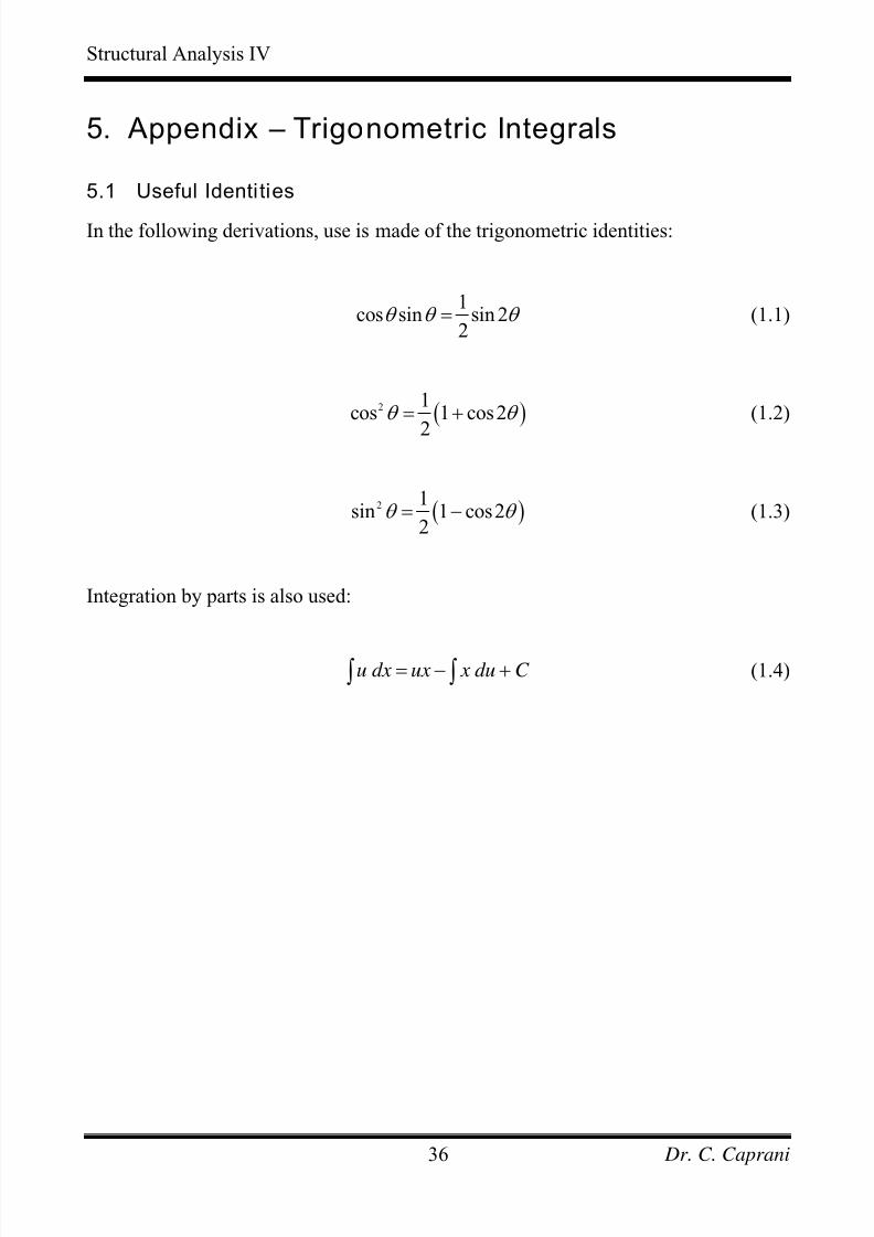
5. Appendix – Trigonometric Integrals
5.1 Useful Identities
In the following derivations, use is made of the trigonometric identities:
1cos sin sin 2
2θ θ = θ (1.1)
(2 1cos 1 cos2
2
)θ θ = + (1.2)
(2 1sin 1 cos2
2)θ θ = − (1.3)
Integration by parts is also used:
u dx ux x du C = − +∫ ∫ (1.4)
Dr. C. Caprani36
7/28/2019 Combined Structures 2009-10
http://slidepdf.com/reader/full/combined-structures-2009-10 37/106
Structural Analysis IV
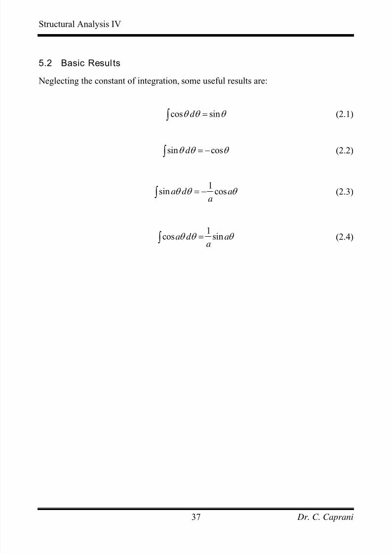
5.2 Basic Resul ts
Neglecting the constant of integration, some useful results are:
cos sind θ θ =∫ θ (2.1)
sin cosd θ θ = −∫ θ (2.2)
1
sin cosa d aaθ θ = −∫ θ (2.3)
1cos sina d a
aθ θ =∫ θ (2.4)
Dr. C. Caprani37
7/28/2019 Combined Structures 2009-10
http://slidepdf.com/reader/full/combined-structures-2009-10 38/106
Structural Analysis IV
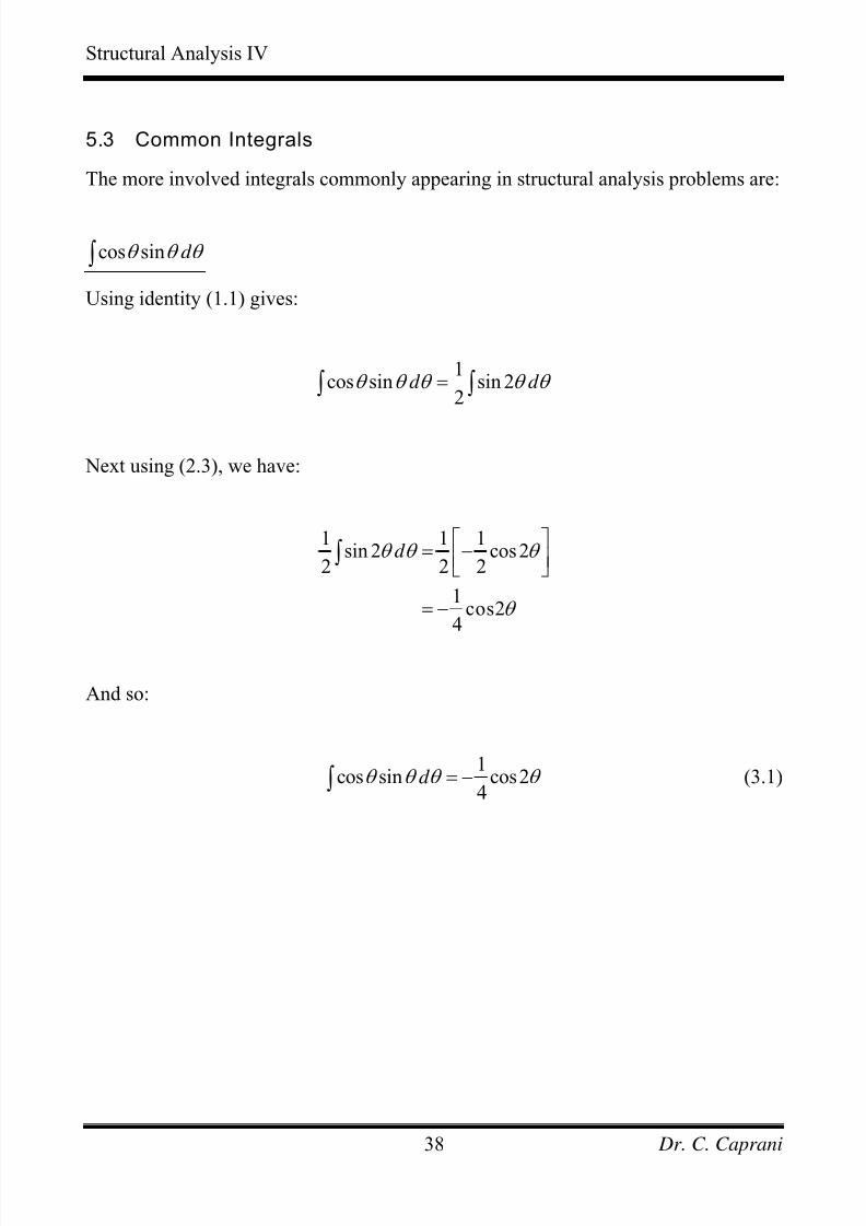
5.3 Common Integrals
The more involved integrals commonly appearing in structural analysis problems are:
cos sin d θ θ θ ∫
Using identity (1.1) gives:
1cos sin sin 2
2d d θ θ θ θ θ =∫ ∫
Next using (2.3), we have:
1 1 1sin 2 cos2
2 2 2
1cos2
4
d θ θ θ
θ
⎡ ⎤= −⎢ ⎥⎣ ⎦
= −
∫
And so:
1cos sin cos2
4d θ θ θ θ = −∫ (3.1)
Dr. C. Caprani38

7/28/2019 Combined Structures 2009-10
http://slidepdf.com/reader/full/combined-structures-2009-10 39/106
Structural Analysis IV
2cos d θ θ ∫
Using (1.2), we have:
( )2 1cos 1 cos2
2
11 cos2
2
d d
d d
θ θ θ θ
θ θ θ
= +
⎡ ⎤= +⎣ ⎦
∫ ∫
∫ ∫
Next using (2.4):
1 11 cos2 sin 2
2 2
1sin2
2 4
d d 1
2θ θ θ θ θ
θ θ
⎡ ⎤⎡ ⎤+ = +⎣ ⎦ ⎢ ⎥⎣ ⎦
= +
∫ ∫
And so:
2 1cos sin 2
2 4d
θ θ θ = +∫ θ (3.2)
Dr. C. Caprani39
7/28/2019 Combined Structures 2009-10
http://slidepdf.com/reader/full/combined-structures-2009-10 40/106
Structural Analysis IV
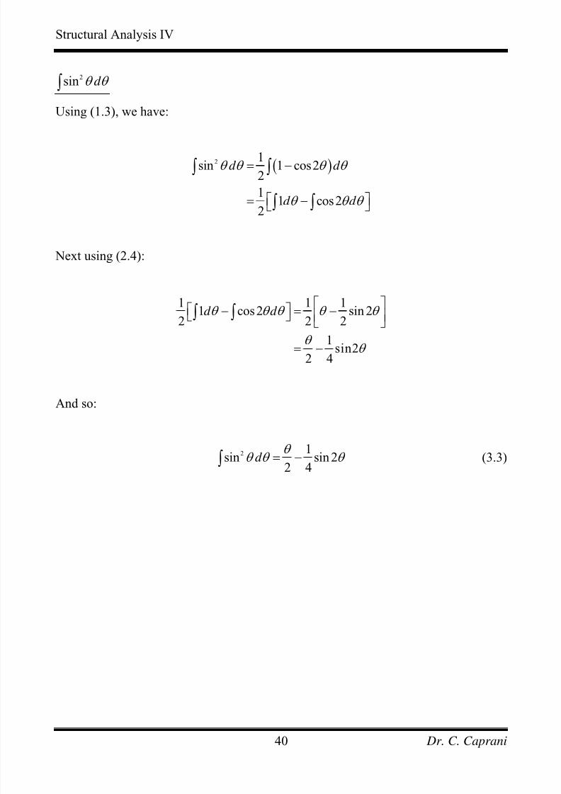
2sin d θ θ ∫
Using (1.3), we have:
( )2 1sin 1 cos2
2
11 cos2
2
d d
d d
θ θ θ θ
θ θ θ
= −
⎡ ⎤= −⎣ ⎦
∫ ∫
∫ ∫
Next using (2.4):
1 11 cos2 sin 2
2 2
1sin2
2 4
d d 1
2θ θ θ θ θ
θ θ
⎡ ⎤⎡ ⎤− = −⎣ ⎦ ⎢ ⎥⎣ ⎦
= −
∫ ∫
And so:
2 1sin sin 2
2 4d
θ θ θ = −∫ θ (3.3)
Dr. C. Caprani40
7/28/2019 Combined Structures 2009-10
http://slidepdf.com/reader/full/combined-structures-2009-10 41/106
Structural Analysis IV
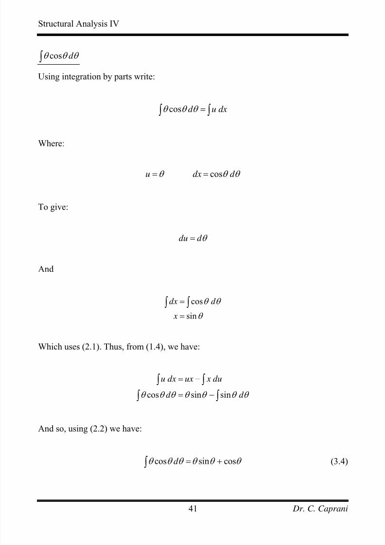
cos d θ θ θ ∫
Using integration by parts write:
cos d u d θ θ θ =∫ ∫ x
d
Where:
cosu dxθ θ θ = =
To give:
du d θ =
And
cos
sin
dx d
x
θ θ
θ
=
=
∫ ∫
Which uses (2.1). Thus, from (1.4), we have:
cos sin sinu dx ux x du
d d θ θ θ θ θ θ θ = −= −
∫ ∫∫ ∫
And so, using (2.2) we have:
cos sin cosd θ θ θ θ θ θ = +∫ (3.4)
Dr. C. Caprani41
7/28/2019 Combined Structures 2009-10
http://slidepdf.com/reader/full/combined-structures-2009-10 42/106
Structural Analysis IV
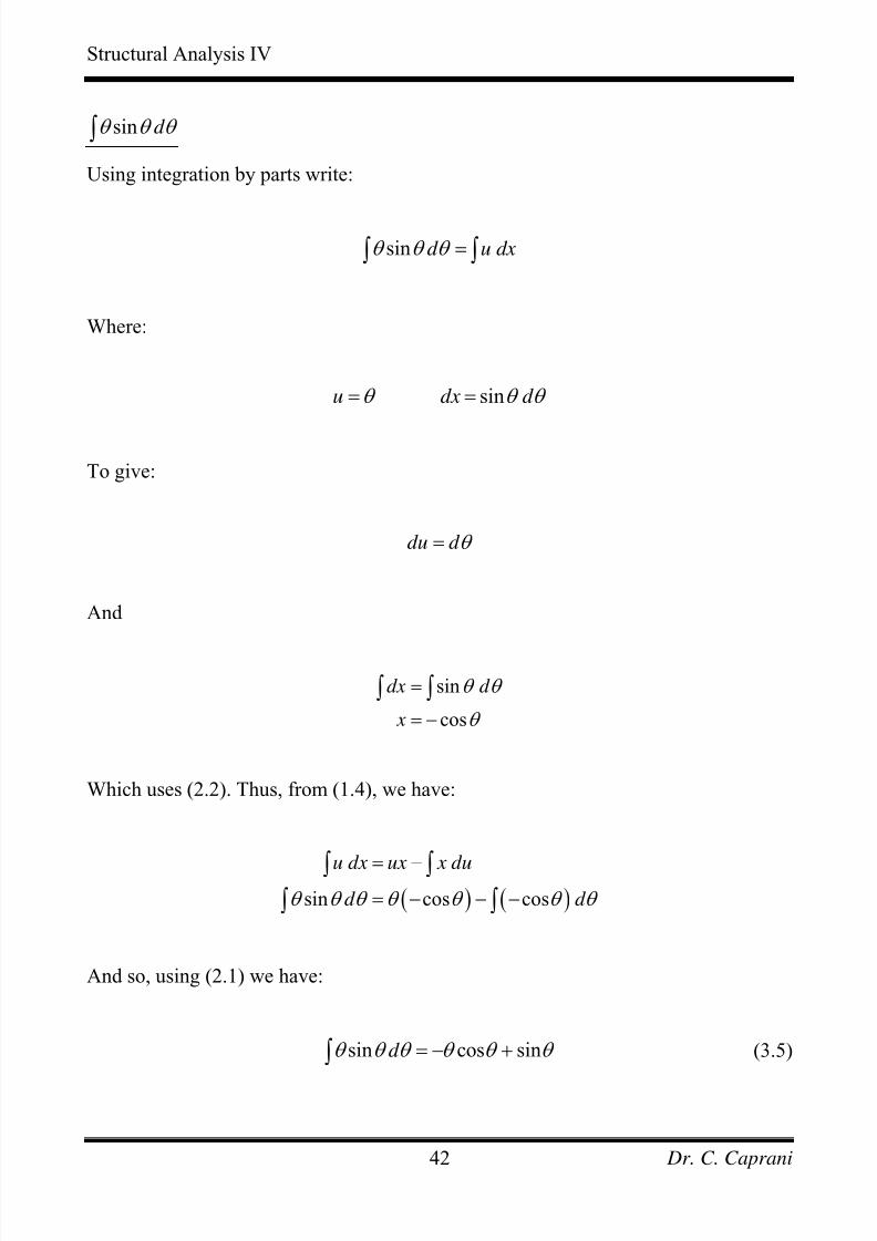
sin d θ θ θ ∫
Using integration by parts write:
sin d u d θ θ θ =∫ ∫ x
d
Where:
sinu dxθ θ θ = =
To give:
du d θ =
And
sin
cos
dx d
x
θ θ
θ
=
= −
∫ ∫
Which uses (2.2). Thus, from (1.4), we have:
( ) ( )sin cos cosu dx ux x du
d d θ θ θ θ θ θ θ = −= − − −
∫ ∫∫ ∫
And so, using (2.1) we have:
sin cos sind θ θ θ θ θ θ = − +∫ (3.5)
Dr. C. Caprani42
7/28/2019 Combined Structures 2009-10
http://slidepdf.com/reader/full/combined-structures-2009-10 43/106
Structural Analysis IV
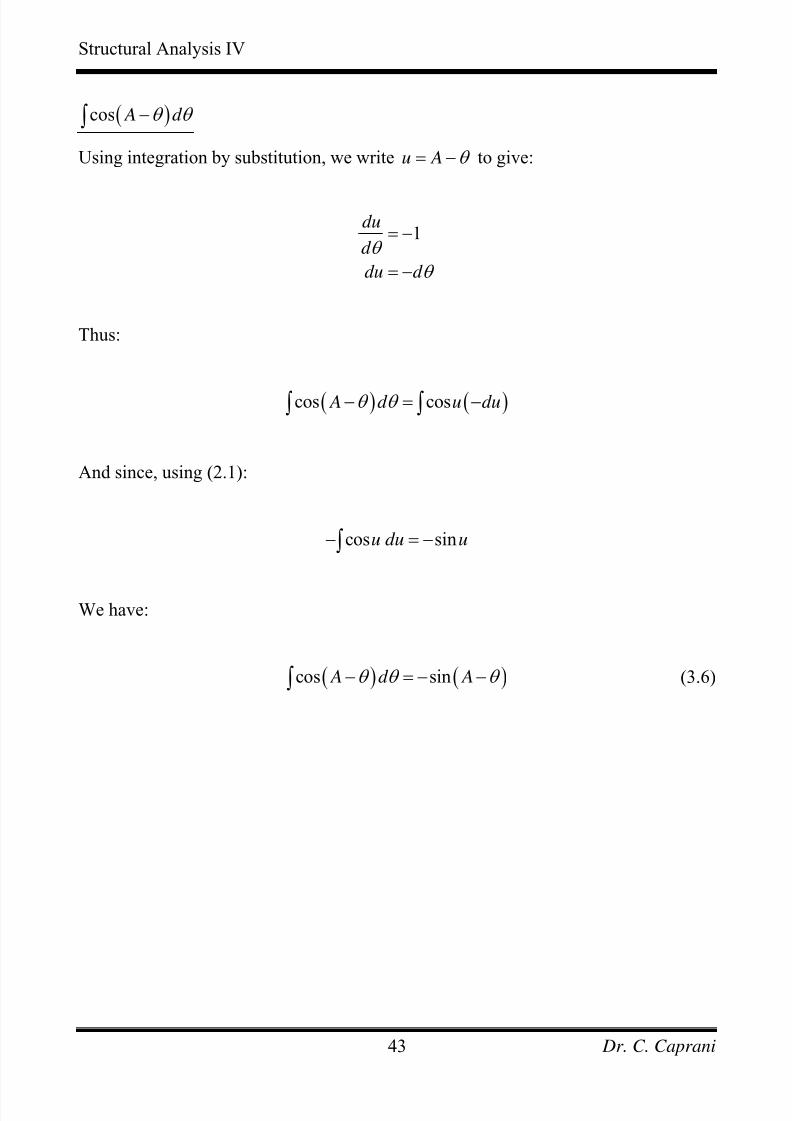
( )cos A d θ θ −∫
Using integration by substitution, we write u A θ = − to give:
1du
d
du d
θ
θ
= −
= −
Thus:
( ) ( )cos cos A d uθ θ − = −∫ ∫ du
And since, using (2.1):
cos sinu du u− = −∫
We have:
( ) ( )cos sin A d Aθ θ θ − = − −∫ (3.6)
Dr. C. Caprani43
7/28/2019 Combined Structures 2009-10
http://slidepdf.com/reader/full/combined-structures-2009-10 44/106
Structural Analysis IV
( )sin A d θ θ −∫
Using integration by substitution, we write u A θ = − to give:
1du
d
du d
θ
θ
= −
= −
Thus:
( ) ( )sin sin A d uθ θ − = −∫ ∫ du
And since, using (2.2):
( )sin cosu du u− = − −∫
We have:
( ) ( )sin cos A d Aθ θ θ − = −∫ (3.7)
Dr. C. Caprani44
7/28/2019 Combined Structures 2009-10
http://slidepdf.com/reader/full/combined-structures-2009-10 45/106
Structural Analysis IV
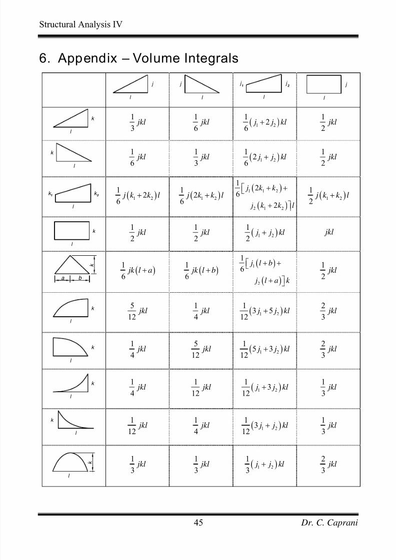
6. Appendix – Volume Integrals
l
j
l
j
l
j j 1 2
l
j
l
k
1
3 jkl 1
6 jkl ( )1 2
12
6 j j+ kl 1
2 jkl
l
k
1
6 jkl 1
3 jkl ( )1 2
12
6 j j k + l 1
2 jkl
l
k k 1 2
( )1 2
1
26 j k k l+ ( )1 2
1
26 j k k + l ( )
( )
1 1 2
2 1 2
12
62
j k k
j k k l
+ +⎡⎣
+ ⎤⎦ ( )1 2
1
2 j k k l+
l
k
1
2 jkl 1
2 jkl ( )1 2
1
2 j j k + l jkl
a b
k
( )
1
6 jk l a+ ( )
1
6 jk l b+ ( )
( )
1
2
1
6 j l b
j l a k
+ +⎡⎣
+ ⎤⎦
1
2 jkl
l
k
5
12 jkl 1
4 jkl ( )1 2
13 5
12 j j+ kl 2
3 jkl
l
k
1
4 jkl 5
12 jkl ( )1 2
15 3
12 j j k + l 2
3 jkl
l
k
1
4 jkl 1
12 jkl ( )
1 2
13
12 j j+ kl 1
3 jkl
l
k
1
12 jkl 1
4 jkl ( )1 2
13
12 j j k + l 1
3 jkl
k
l 1
3 jkl 1
3 jkl ( )1 2
1
3 j j k + l 2
3 jkl
Dr. C. Caprani45
7/28/2019 Combined Structures 2009-10
http://slidepdf.com/reader/full/combined-structures-2009-10 46/106
Structural Analysis IV
7. Ring Beam Examples (Advanced)
7.1 Example 1
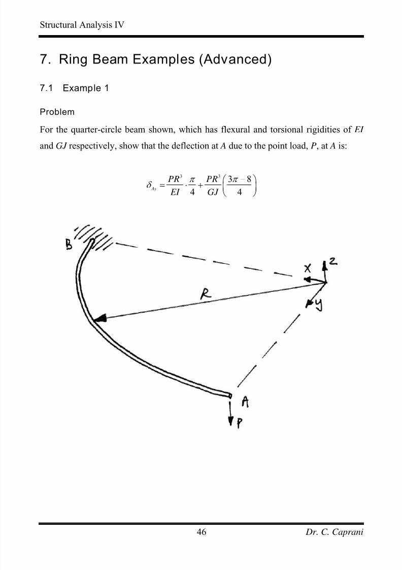
Problem
For the quarter-circle beam shown, which has flexural and torsional rigidities of EI
and GJ respectively, show that the deflection at A due to the point load, P, at A is:
3 3 3 8
4 4 Ay
PR PR
EI GJ
π π δ
−⎛ = ⋅ + ⎜
⎝ ⎠
⎞⎟
Dr. C. Caprani46
7/28/2019 Combined Structures 2009-10
http://slidepdf.com/reader/full/combined-structures-2009-10 47/106
Structural Analysis IV
Solution
The point load will cause both bending and torsion in the beam member. Therefore
both effects must be accounted for in the deflection calculations. Shear effects are
ignored.
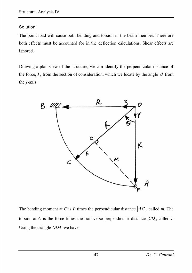
Drawing a plan view of the structure, we can identify the perpendicular distance of
the force, P, from the section of consideration, which we locate by the angle θ from
the y-axis:
The bending moment at C is P times the perpendicular distance AC , called m. The
torsion at C is the force times the transverse perpendicular distance CD , called t .
Using the triangle ODA, we have:
Dr. C. Caprani47
7/28/2019 Combined Structures 2009-10
http://slidepdf.com/reader/full/combined-structures-2009-10 48/106
Structural Analysis IV
sin sin
cos cos
mm R
R
ODOD R
R
θ θ
θ θ
= ∴ =
= ∴ =
The distance CD , or t , is R OD− , thus:
( )
cos
1 cos
t R OD
R R
R
θ
θ
= −
= −
= −
Thus the bending moment at point C is:
( )
sin
M Pm
PR
θ
θ
=
=(1.1)
The torsion at C is:
( )
( )1 cos
T Pt
PR
θ
θ
=
= −(1.2)
Using virtual work, we have:
0
E I
Ay
W
W W
M T F M ds T ds
EI GJ
δ
δ δ
δ δ δ δ
=
=
⋅ = ⋅ + ⋅∫ ∫
(1.3)
Dr. C. Caprani48
7/28/2019 Combined Structures 2009-10
http://slidepdf.com/reader/full/combined-structures-2009-10 49/106
Structural Analysis IV
This equation represents the virtual work done by the application of a virtual force,
F δ , in the vertical direction at A, with its internal equilibrium virtual moments and
torques, M δ and T δ and so is the equilibrium system. The compatible
displacements system is that of the actual deformations of the structure, externally at
A, and internally by the curvatures and twists, M EI and T GJ .
Taking the virtual force, 1F δ = , and since it is applied at the same location and
direction as the actual force P, we have, from equations (1.1) and (1.2):
( ) sin M Rδ θ θ = (1.4)
( ) ( )1 cosT Rδ θ θ = − (1.5)
Thus, the virtual work equation, (1.3), becomes:
[ ][ ] ( ) ( )2 2
0 0
1 11
1 1sin sin 1 cos 1 cos
Ay M M ds T T ds EI GJ
PR R Rd PR R Rd EI GJ
π π
δ δ δ
θ θ θ θ θ
⋅ = ⋅ + ⋅
= + −⎡ ⎤ ⎡⎣ ⎦ ⎣
∫ ∫
∫ ∫ θ − ⎤⎦
(1.6)
In which we have related the curve distance, , to the arc distance, dsds Rd θ = , which
allows us to integrate round the angle rather than along the curve. Multiplying out:
( )2 23 3
22
0 0
sin 1 cos Ay
PR PRd
EI GJ
π π
d δ θ θ θ θ = + −∫ ∫ (1.7)
Considering the first term, from the integrals’ appendix, we have:
Dr. C. Caprani49
7/28/2019 Combined Structures 2009-10
http://slidepdf.com/reader/full/combined-structures-2009-10 50/106
Structural Analysis IV
( )
22
2
00
1sin sin 2
2 4
1
0 0 04 4
4
d
π π θ
θ θ θ
π
π
⎡ ⎤= −⎢ ⎥⎣ ⎦
⎡ ⎤⎛ ⎞= − ⋅ − −
⎜ ⎟⎢ ⎥⎝ ⎠⎣ ⎦
=
∫
(1.8)
The second term is:
( ) ( )2 2
2 2
0 0
2 2 2
2
0 0 0
1 cos 1 2cos cos
1 2 cos cos
d d
d d
π π
π π π
θ θ θ θ θ
d θ θ θ θ θ
− = − +
= − +
∫ ∫
∫ ∫ ∫
(1.9)
Thus, from the integrals in the appendix:
( ) [ ] [ ]
( ) ( ) ( ) ( )
222 22
0 000
11 cos 2 sin sin 2
2 4
10 2 1 0 0 0 0
2 4 4
22 4
3 8
4
d
π π π π θ
θ θ θ θ θ
π π
π π
π
⎡ ⎤− = − + +⎢ ⎥⎣ ⎦
⎡ ⎤ ⎡⎛ ⎞ ⎛ ⎞= − − − + + ⋅ − +⎡ ⎤⎜ ⎟ ⎜ ⎟⎢ ⎥ ⎢⎣ ⎦
⎝ ⎠ ⎝ ⎠⎣ ⎦ ⎣
= − +
−
=
∫
⎤⎥⎦ (1.10)
Substituting these results back into equation (1.7) gives the desired result:
3 3 3 8
4 4 Ay
PR PR
EI GJ
π π δ
−⎛ = + ⎜
⎝ ⎠
⎞⎟ (1.11)
Dr. C. Caprani50
7/28/2019 Combined Structures 2009-10
http://slidepdf.com/reader/full/combined-structures-2009-10 51/106
Structural Analysis IV
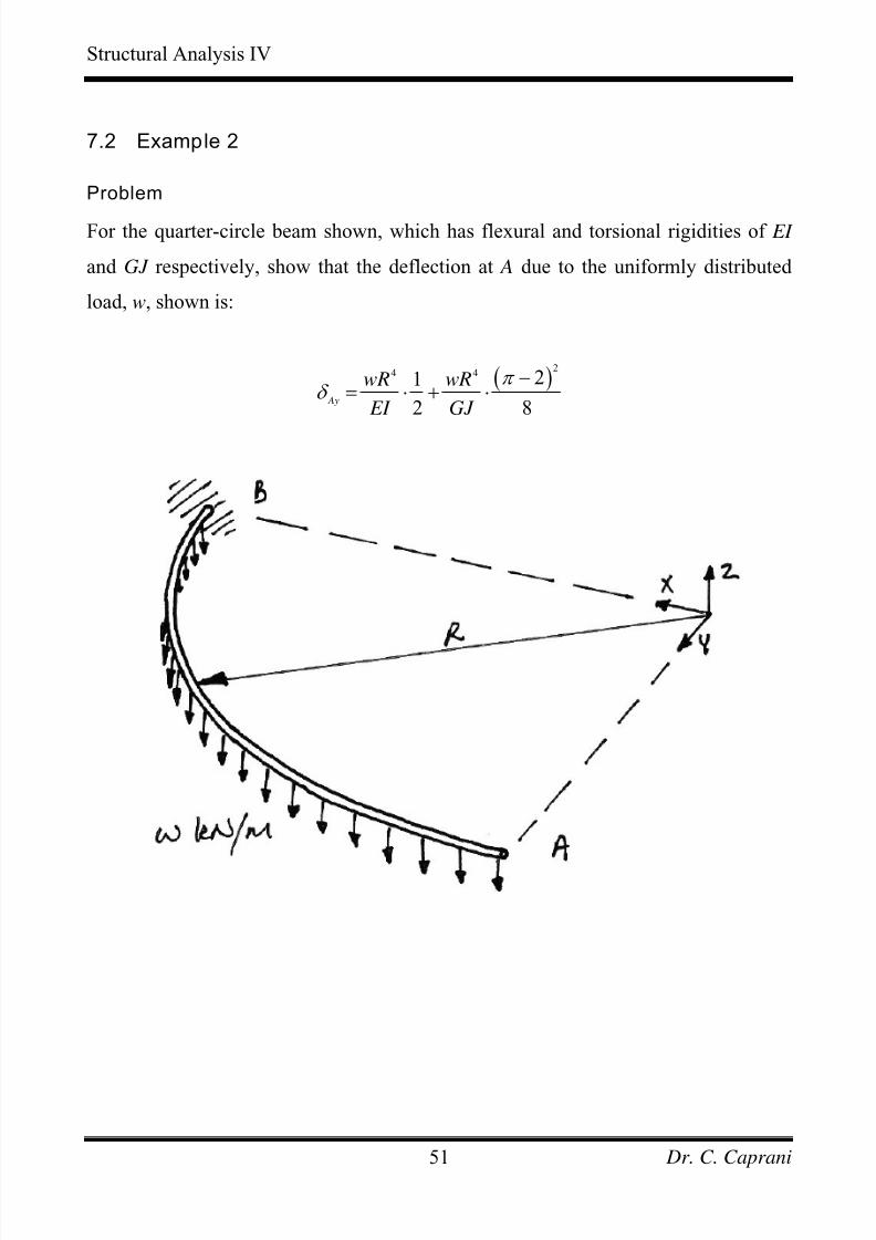
7.2 Example 2
Problem
For the quarter-circle beam shown, which has flexural and torsional rigidities of EI
and GJ respectively, show that the deflection at A due to the uniformly distributed
load, w, shown is:
( )2
4 4 21
2 8 Ay
wR wR
EI GJ
π δ
−= ⋅ + ⋅
Dr. C. Caprani51
7/28/2019 Combined Structures 2009-10
http://slidepdf.com/reader/full/combined-structures-2009-10 52/106
Structural Analysis IV
Solution
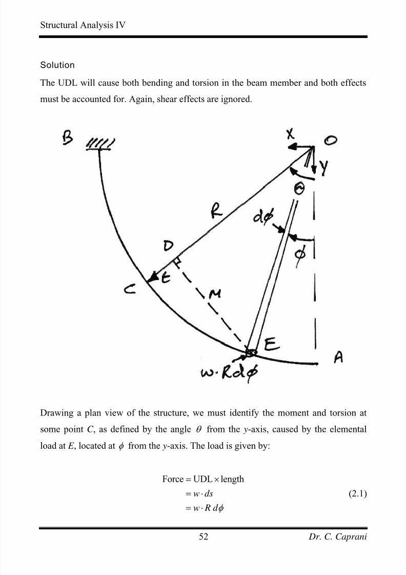
The UDL will cause both bending and torsion in the beam member and both effects
must be accounted for. Again, shear effects are ignored.
Drawing a plan view of the structure, we must identify the moment and torsion at
some point C , as defined by the angle θ from the y-axis, caused by the elemental
load at E , located at φ from the y-axis. The load is given by:
Force UDL length
w ds
w R d φ
= ×
= ⋅
= ⋅
(2.1)
Dr. C. Caprani52
7/28/2019 Combined Structures 2009-10
http://slidepdf.com/reader/full/combined-structures-2009-10 53/106
Structural Analysis IV
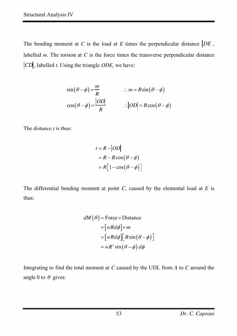
The bending moment at C is the load at E times the perpendicular distance DE ,
labelled m. The torsion at C is the force times the transverse perpendicular distance
CD , labelled t . Using the triangle ODE , we have:
( ) ( )
( ) ( )
sin sin
cos cos
mm R
R
ODOD R
R
θ φ θ φ
θ φ θ
− = ∴ = −
− = ∴ = − φ
The distance t is thus:
( )
( )
cos
1 cos
t R OD
R R
R
θ φ
θ φ
= −
= − −
= − −⎡ ⎤⎣ ⎦
The differential bending moment at point C , caused by the elemental load at E is
thus:
( )
[ ]
[ ] ( )( )2
Force Distance
sin
sin
dM
wRd m
wRd R
wR d
θ
φ
φ θ φ
θ φ φ
= ×
= ×
= −⎡ ⎤⎣ ⎦
= −
Integrating to find the total moment at C caused by the UDL from A to C around the
angle 0 to θ gives:
Dr. C. Caprani53
7/28/2019 Combined Structures 2009-10
http://slidepdf.com/reader/full/combined-structures-2009-10 54/106
Structural Analysis IV
( ) ( )
( )
( )
2
0
2
0
sin
sin
M dM
wR d
wR d
φ θ
φ
φ θ
φ
θ θ
θ φ φ
θ φ φ
=
=
=
=
=
= −
= −
∫
∫
∫
In this integral θ is a constant and only φ is considered a variable. Using the identity
from the integral table gives:
( ) ( )
( )
2
0
2
cos
cos0 cos
M wR
wR
φ θ
φ θ θ φ
θ
=
== −⎡ ⎤⎣ ⎦
= −⎡ ⎤⎣ ⎦
And so:
( ) ( )2 1 cos M wRθ θ = − (2.2)
Along similar lines, the torsion at C caused by the load at E is:
( ) [ ]
[ ] ( ){
( )
2
1 cos
1 cos
dT wRd t
wRd R
wR d
}
θ φ
φ θ φ
θ φ φ
= ×
= − −⎡ ⎤⎣ ⎦
= − −⎡ ⎤⎣ ⎦
And integrating for the total torsion at C :
Dr. C. Caprani54
7/28/2019 Combined Structures 2009-10
http://slidepdf.com/reader/full/combined-structures-2009-10 55/106
Structural Analysis IV
( ) ( )
( )
( )
( )
2
0
2
0
2
0 0
1 cos
1 cos
1 cos
T dT
wR d
wR d
wR d d
φ θ
φ
φ θ
φ
φ θ φ θ
φ φ
θ θ
θ φ φ
θ φ φ
φ θ φ φ
=
=
=
=
= =
= =
=
= − −⎡ ⎤⎣ ⎦
= − −⎡ ⎤⎣ ⎦
⎧ ⎫= − −⎨ ⎬
⎩ ⎭
∫
∫
∫
∫ ∫
Using the integral identity for ( )cos θ φ − gives:
( ) [ ] ( ){ }[ ]{ }
2
0 0
2
sin
sin 0 sin
T wR
wR
φ θ φ θ
φ φ θ φ θ φ
θ θ
==
= == − − −⎡ ⎤⎣ ⎦
= + −
And so the total torsion at C is:
( ) ( )2 sinT wRθ θ θ = − (2.3)
To determine the deflection at A, we apply a virtual force, F δ , in the vertical
direction at A. Along with its internal equilibrium virtual moments and torques, M δ
and T δ and this set forms the equilibrium system. The compatible displacements
system is that of the actual deformations of the structure, externally at A, and
internally by the curvatures and twists, M EI and T GJ . Therefore, using virtual
work, we have:
0
E I
Ay
W
W W
M T F M ds T ds
EI GJ
δ
δ δ
δ δ δ δ
=
=
⋅ = ⋅ + ⋅∫ ∫
(2.4)
Dr. C. Caprani55
7/28/2019 Combined Structures 2009-10
http://slidepdf.com/reader/full/combined-structures-2009-10 56/106
Structural Analysis IV
Taking the virtual force, 1F δ = , and using the equation for moment and torque at
any angle θ from Example 1, we have:
( ) sin M Rδ θ θ = (2.5)
( ) ( )1 cosT Rδ θ θ = − (2.6)
Thus, the virtual work equation, (2.4), using equations (2.2) and (2.3), becomes:
( ) [ ]
( ) ( )
2
2
0
2
2
0
1 11
11 cos sin
1sin 1 cos
Ay M M ds T T ds EI GJ
wR R Rd EI
wR R Rd GJ
π
π
δ δ δ
θ θ θ
θ θ θ
⋅ = ⋅ + ⋅
⎡ ⎤= −⎣ ⎦
⎡ ⎤+ − −⎡ ⎤⎣ ⎦⎣ ⎦
∫ ∫
∫
∫ θ
(2.7)
In which we have related the curve distance, , to the arc distance,ds ds Rd θ =
allowing us to integrate round the angle rather than along the curve. Multiplying out:
( )
( )
24
0
24
0
sin sin cos
sin cos cos sin
Ay
wRd
EI
wRd
GJ
π
π
δ θ θ θ θ
θ θ θ θ θ θ θ
= −
+ − − +
∫
∫(2.8)
Using the respective integrals from the appendix yields:
Dr. C. Caprani56
7/28/2019 Combined Structures 2009-10
http://slidepdf.com/reader/full/combined-structures-2009-10 57/106
Structural Analysis IV
( )
( ) ( )
24
0
24 2
0
4
4 2
4
4 2
1cos cos2
4
1cos sin cos cos2
2 4
1 10 1
4 4
1 10 1 0 1 0 1 0 1
8 2 4 4
1
2
1 1
8 2 4 4
Ay
wR
EI
wR
GJ
wR
EI
wR
GJ
wR
EI
wR
GJ
π
π
δ θ θ
θ θ θ θ θ θ
π π
π π
⎡ ⎤= − +⎢ ⎥⎣ ⎦
⎡ ⎤+ + − + −
⎢ ⎥⎣ ⎦
⎡ ⎤⎛ ⎞ ⎛ ⎞= − − − − +⎜ ⎟ ⎜ ⎟⎢ ⎥
⎝ ⎠ ⎝ ⎠⎣ ⎦
⎡ ⎤⎛ ⎞⎛ ⎞ ⎛ + + − ⋅ + − − − + − + −⎢ ⎥⎜ ⎟⎜ ⎟ ⎜
⎝ ⎠ ⎝ ⎝ ⎠⎣ ⎦
⎡ ⎤= ⎢ ⎥⎣ ⎦
⎡+ − + +⎣
⎤⎢ ⎥⎦
⎞⎟
⎠
Writing the second term as a common fraction:
4 4 21 4
2 8
Ay
wR wR
EI GJ
π π δ
⎛ 4 ⎞− += ⋅ + ⎜
⎝ ⎠
⎟
And then factorising, gives the required deflection at A:
( )2
24 4 21
2 8 Ay
wR wR
EI GJ
π δ
−= ⋅ + ⋅ (2.9)
Dr. C. Caprani57
7/28/2019 Combined Structures 2009-10
http://slidepdf.com/reader/full/combined-structures-2009-10 58/106
Structural Analysis IV
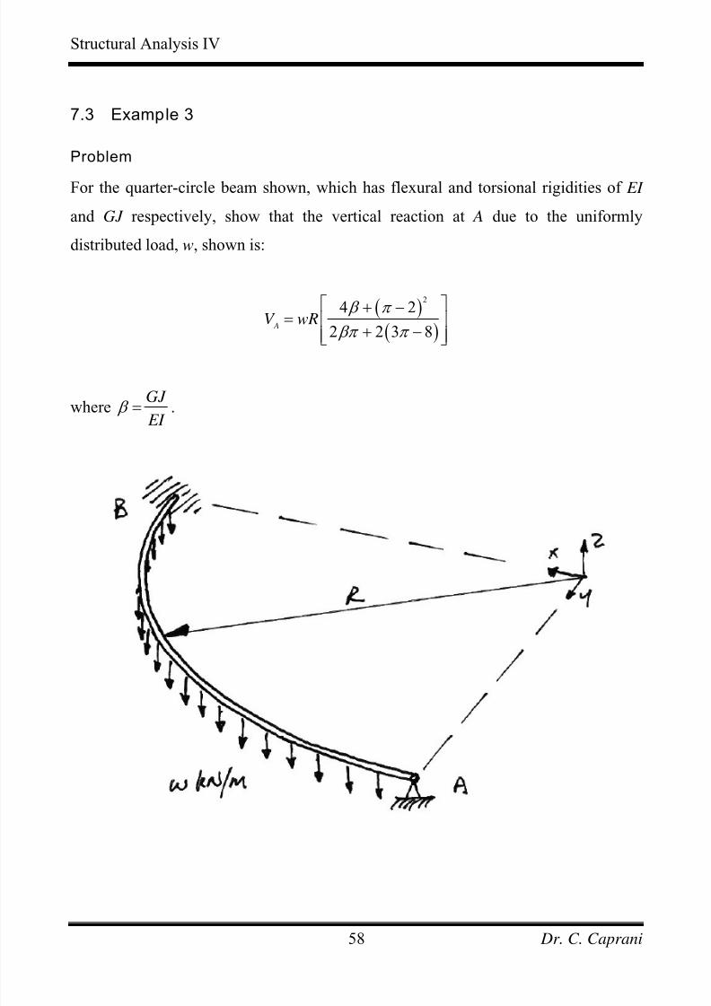
7.3 Example 3
Problem
For the quarter-circle beam shown, which has flexural and torsional rigidities of EI
and GJ respectively, show that the vertical reaction at A due to the uniformly
distributed load, w, shown is:
( )( )
2
4 2
2 2 3 8 A
V wR β π
βπ π
⎡ ⎤+ −= ⎢ ⎥
+ −⎢ ⎥⎣ ⎦
whereGJ
EI β = .
Dr. C. Caprani58
7/28/2019 Combined Structures 2009-10
http://slidepdf.com/reader/full/combined-structures-2009-10 59/106
Structural Analysis IV
Solution
This problem can be solved using two apparently different methods, but which are
equivalent. Indeed, examining how they are equivalent leads to insights that make
more difficult problems easier, as we shall see in subsequent problems. For both
approaches we will make use of the results obtained thus far:
• Deflection at A due to UDL:
( )2
4 4 21
2 8
Ay
wR wR
EI GJ
π δ
−= ⋅ + ⋅ (3.1)
• Deflection at A due to point load at A:
3 3 3 8
4 4 Ay
PR PR
EI GJ
π π δ
−⎛ = ⋅ + ⎜
⎝ ⎠
⎞⎟ (3.2)
Using Compatibility of Displacement
The basic approach, which does not require virtual work, is to use compatibility of
displacement in conjunction with superposition. If we imagine the support at A
removed, we will have a downwards deflection at A caused by the UDL, which
equation (3.1) gives us as:
( )2
4 4
021
2 8 Ay
wR wR
EI GJ
π δ
−= ⋅ + ⋅ (3.3)
As illustrated in the following diagram.
Dr. C. Caprani59
7/28/2019 Combined Structures 2009-10
http://slidepdf.com/reader/full/combined-structures-2009-10 60/106
Structural Analysis IV
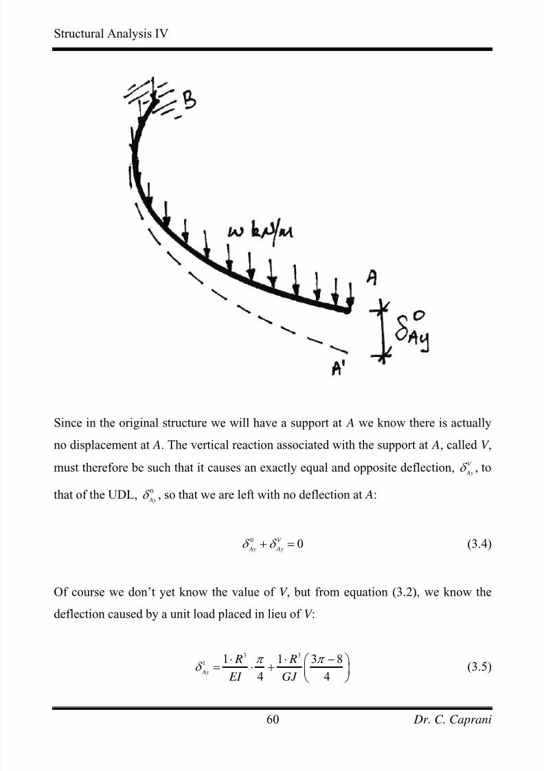
Since in the original structure we will have a support at A we know there is actually
no displacement at A. The vertical reaction associated with the support at A, called V ,
must therefore be such that it causes an exactly equal and opposite deflection, V
Ayδ , to
that of the UDL, 0
Ayδ , so that we are left with no deflection at A:
0 0V Ay Ayδ δ + = (3.4)
Of course we don’t yet know the value of V , but from equation (3.2), we know the
deflection caused by a unit load placed in lieu of V :
3 3
1 1 1 3
4 4 Ay
R R
EI GJ
π π δ
8⋅ ⋅ −⎛ = ⋅ + ⎜
⎝ ⎠
⎞⎟ (3.5)
Dr. C. Caprani60
7/28/2019 Combined Structures 2009-10
http://slidepdf.com/reader/full/combined-structures-2009-10 61/106
Structural Analysis IV
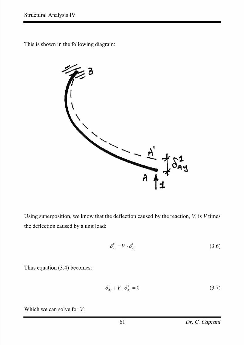
This is shown in the following diagram:
Using superposition, we know that the deflection caused by the reaction, V , is V times
the deflection caused by a unit load:
1V
Ay AyV δ δ = ⋅ (3.6)
Thus equation (3.4) becomes:
0 1 0 Ay Ay
V δ δ + ⋅ = (3.7)
Which we can solve for V :
Dr. C. Caprani61
7/28/2019 Combined Structures 2009-10
http://slidepdf.com/reader/full/combined-structures-2009-10 62/106
Structural Analysis IV
0
1
Ay
Ay
V δ
δ = − (3.8)
If we take downwards deflections to be positive, we then have, from equations(3.3),
(3.5), and (3.8):
( )2
4 4
3 3
21
2 8
1 1 3
4 4
wR wR
EI GJ
V R R
EI GJ
π
π π
⎛ ⎞−⋅ + ⋅⎜ ⎟⎜ ⎟
⎝
= − ⎡ ⋅ ⋅ − ⎤⎛ ⎞− ⋅ + ⎜ ⎟⎢ ⎥⎝ ⎠⎣ ⎦
8
⎠(3.9)
The two negative signs cancel, leaving us with a positive value for V indicating that it
is in the same direction as the unit load, and so is upwards as expected. Introducing
GJ
EI
β = and doing some algebra on equation (3.9) gives:
( )
( )
( ) ( )
( )( )
12
12
12
2
21 1 1 1 1 3 8
2 8 4 4
21 1 1 3 8
2 8 4 4
4 2 3 88 4
4 2 8
8 2 2 3 8
V wR EI EI EI EI
wR
wR
wR
π π π
β β
π π π
β β
β π βπ π β β
β π β
β βπ π
−
−
−
⎛ ⎞− ⎡ ⎤−⎛ ⎞= ⋅ + ⋅ × ⋅ +⎜ ⎟ ⎜ ⎟⎢ ⎥⎜ ⎟ ⎝ ⎠⎣ ⎦⎝ ⎠
⎛ ⎞− ⎡ ⎤−⎛ ⎞= + ⋅ × +⎜ ⎟ ⎜ ⎟⎢ ⎥⎜ ⎟ ⎝ ⎠⎣ ⎦⎝ ⎠
⎛ ⎞+ − + −⎡ ⎤= ×⎜ ⎟ ⎢ ⎥⎜ ⎟ ⎣ ⎦⎝ ⎠
⎛ ⎞ ⎡ ⎤+ −= ×⎜ ⎟ ⎢ ⎥⎜ ⎟ + −⎣ ⎦⎝ ⎠
And so we finally have the required reaction at A as:
Dr. C. Caprani62
7/28/2019 Combined Structures 2009-10
http://slidepdf.com/reader/full/combined-structures-2009-10 63/106
Structural Analysis IV
( )( )
2
4 2
2 2 3 8 A
V wR β π
βπ π
⎛ ⎞+ −= ⎜⎜ + −⎝ ⎠
⎟⎟
ds
(3.10)
Using Virtual Work
To calculate the reaction at A using virtual work, we use the following:
• Equilibrium system: the external and internal virtual forces corresponding to a
unit virtual force applied in lieu of the required reaction;
• Compatible system: the real external and internal displacements of the original
structure subject to the real applied loads.
Thus the virtual work equations are:
0
E I
Ay
W
W W
F M ds T
δ
δ δ
δ δ κ δ φ δ
=
=
⋅ = ⋅ + ⋅∫ ∫
(3.11)
At this point we introduce some points:
• The real external deflection at A is zero: 0 Ay
δ = ;
• The virtual force, 1F δ = ;
• The real curvatures can be expressed using the real bending moments, M
EI κ = ;
• The real twists are expressed from the torque,
T
GJ φ = .
These combine to give, from equation (3.11):
0 0
0 1 L L
M T M ds T ds
EI GJ δ
⎡ ⎤ ⎡ ⎤⋅ = ⋅ + ⋅⎢ ⎥ ⎢ ⎥⎣ ⎦ ⎣ ⎦
∫ ∫ δ (3.12)
Dr. C. Caprani63
7/28/2019 Combined Structures 2009-10
http://slidepdf.com/reader/full/combined-structures-2009-10 64/106
Structural Analysis IV
Next, we use superposition to express the real internal ‘forces’ as those due to the real
loading applied to the primary structure plus a multiplier times those due to the unit
virtual load applied in lieu of the reaction:
0 1 0 1 M M M T T T α α = + = + (3.13)
Notice that 1 M M δ = and 1
T T δ = , but they are still written with separate notation to
keep the ideas clear. Thus equation (3.12) becomes:
( ) ( )0 1 0 1
0 0
0 1 0 1
0 0 0 0
0
0
L L
L L L L
M M T T M ds T ds
EI GJ
M M T T M ds M ds T ds T ds
EI EI GJ GJ
α α δ δ
δ α δ δ α δ
⎡ ⎤ ⎡ ⎤+ += ⋅ + ⋅⎢ ⎥ ⎢ ⎥
⎢ ⎥ ⎢ ⎥⎣ ⎦ ⎣ ⎦
= ⋅ + ⋅ ⋅ + ⋅ + ⋅ ⋅
∫ ∫
∫ ∫ ∫ ∫
(3.14)
And so finally:
0 0
0 0
1 1
0 0
L L
L L
M T M ds T ds
EI GJ
M T M ds T ds
EI GJ
δ δ
α
δ δ
⎡ ⎤⋅ + ⋅⎢ ⎥
⎣= −⎡ ⎤
⋅ + ⋅⎢ ⎥⎣ ⎦
∫ ∫
∫ ∫
⎦ (3.15)
At this point we must note the similarity between equations (3.15) and (3.8). From
equation (1.3), it is clear that the numerator in equation (3.15) is the deflection at A of
the primary structure subject to the real loads. Further, from equation (2.4), the
denominator in equation (3.15) is the deflection at A due to a unit (virtual) load at A.
Neglecting signs, and generalizing somewhat, we can arrive at an ‘empirical’
equation for the calculation of redundants:
Dr. C. Caprani64
7/28/2019 Combined Structures 2009-10
http://slidepdf.com/reader/full/combined-structures-2009-10 65/106
Structural Analysis IV
of primary structure alongdue to actual loads
line of action of redundantdue to unit redundant
δ α
δ
⎫= ⎬
⎭(3.16)
Using this form we will quickly be able to determine the solutions to further ring-
beam problems.
The solution for α follows directly from the previous examples:
• The numerator is determined as per Example 1;
• The denominator is determined as per Example 2, with 1P = .
Of course, these two steps give the results of equations (3.3) and (3.5) which were
used in equation (3.8) to obtain equation (3.9), and leading to the solution, equation
(3.10).
From this it can be seen that compatibility of displacement and virtual work are
equivalent ways of looking at the problem. Also it is apparent that the virtual work
framework inherently calculates the displacements required in a compatibility
analysis. Lastly, equation (3.16) provides a means for quickly calculating the
redundant for other arrangements of the structure from the existing solutions, as will
be seen in the next example.
Dr. C. Caprani65
7/28/2019 Combined Structures 2009-10
http://slidepdf.com/reader/full/combined-structures-2009-10 66/106
Structural Analysis IV
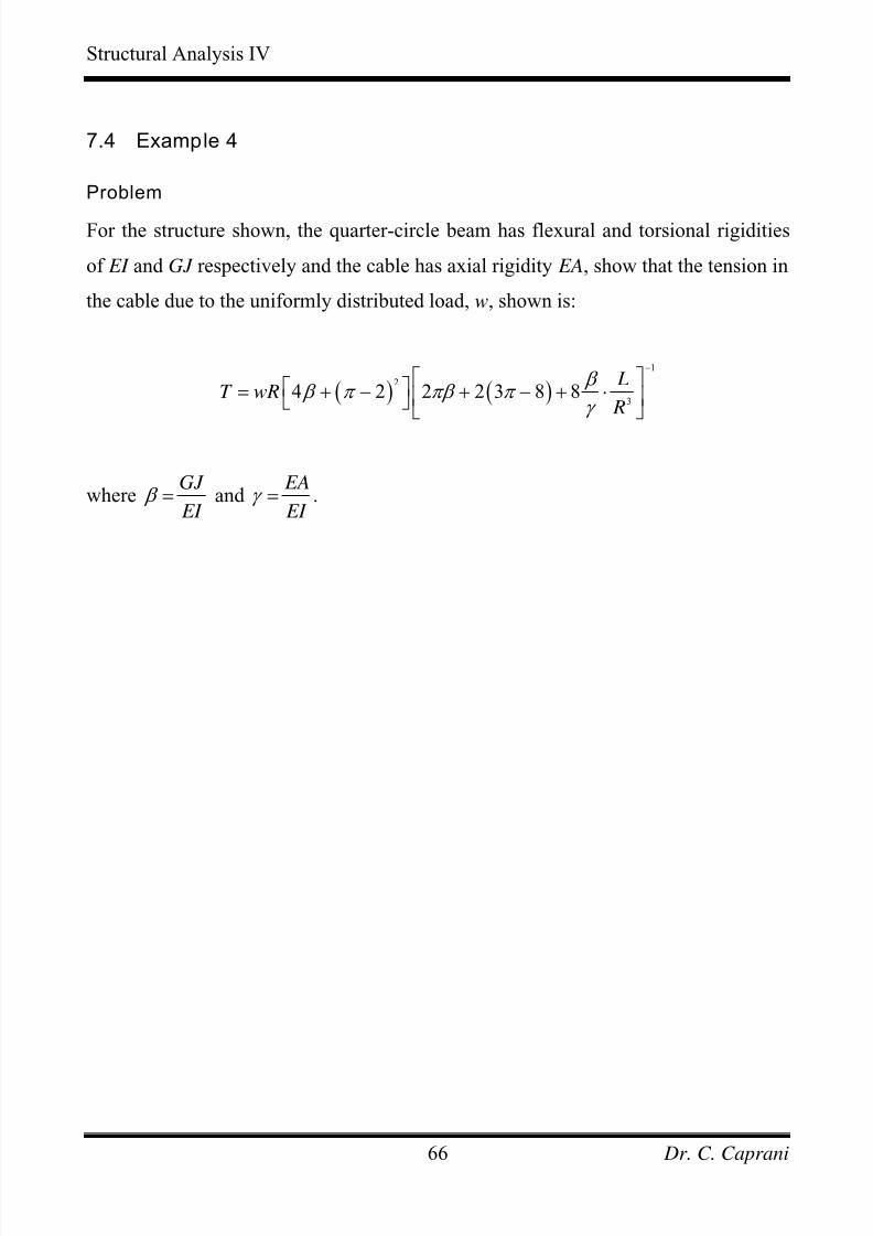
7.4 Example 4
Problem
For the structure shown, the quarter-circle beam has flexural and torsional rigidities
of EI and GJ respectively and the cable has axial rigidity EA, show that the tension in
the cable due to the uniformly distributed load, w, shown is:
( ) ( )1
2
34 2 2 2 3 8 8
LT wR
R
β β π πβ π
γ
−
⎡ ⎤⎡ ⎤= + − + − + ⋅⎢ ⎥⎣ ⎦ ⎣ ⎦
whereGJ
EI β = and
EA
EI γ = .
Dr. C. Caprani66

7/28/2019 Combined Structures 2009-10
http://slidepdf.com/reader/full/combined-structures-2009-10 67/106
Structural Analysis IV
Dr. C. Caprani67
7/28/2019 Combined Structures 2009-10
http://slidepdf.com/reader/full/combined-structures-2009-10 68/106
Structural Analysis IV
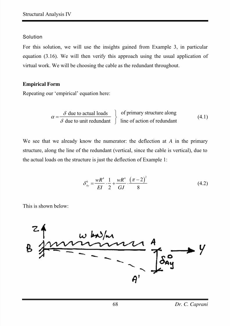
Solution
For this solution, we will use the insights gained from Example 3, in particular
equation (3.16). We will then verify this approach using the usual application of
virtual work. We will be choosing the cable as the redundant throughout.
Empirical Form
Repeating our ‘empirical’ equation here:
of primary structure alongdue to actual loads line of action of redundantdue to unit redundant
δ α δ
⎫= ⎬⎭
(4.1)
We see that we already know the numerator: the deflection at A in the primary
structure, along the line of the redundant (vertical, since the cable is vertical), due to
the actual loads on the structure is just the deflection of Example 1:
( )2
4 4
021
2 8 Ay
wR wR
EI GJ
π δ
−= ⋅ + ⋅ (4.2)
This is shown below:
Dr. C. Caprani68
7/28/2019 Combined Structures 2009-10
http://slidepdf.com/reader/full/combined-structures-2009-10 69/106
Structural Analysis IV
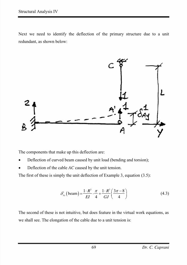
Next we need to identify the deflection of the primary structure due to a unit
redundant, as shown below:
The components that make up this deflection are:
• Deflection of curved beam caused by unit load (bending and torsion);
• Deflection of the cable AC caused by the unit tension.
The first of these is simply the unit deflection of Example 3, equation (3.5):
( )3 3
1 1 1 3 beam
4 4 Ay
R R
EI GJ
π π δ
8⋅ ⋅ −⎛ = ⋅ + ⎜
⎝ ⎠
⎞⎟ (4.3)
The second of these is not intuitive, but does feature in the virtual work equations, as
we shall see. The elongation of the cable due to a unit tension is:
Dr. C. Caprani69
7/28/2019 Combined Structures 2009-10
http://slidepdf.com/reader/full/combined-structures-2009-10 70/106
Structural Analysis IV
( )1 1cable
Ay
L
EAδ
⋅= (4.4)
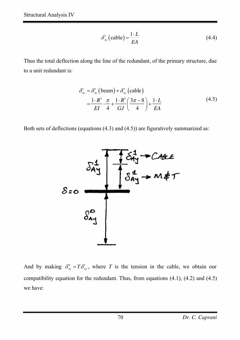
Thus the total deflection along the line of the redundant, of the primary structure, due
to a unit redundant is:
( ) ( )1 1 1
3 3
beam cable
1 1 3 8
4 4
Ay Ay Ay
1 R R L
EI GJ
δ δ δ
π π
= +
⋅ ⋅ −⎛ ⎞= ⋅ + +⎜ ⎟
⎝ ⎠ EA
⋅ (4.5)
Both sets of deflections (equations (4.3) and (4.5)) are figuratively summarized as:
And by making 0
Ay AyT
1δ δ = , where T is the tension in the cable, we obtain our
compatibility equation for the redundant. Thus, from equations (4.1), (4.2) and (4.5)
we have:
Dr. C. Caprani70
7/28/2019 Combined Structures 2009-10
http://slidepdf.com/reader/full/combined-structures-2009-10 71/106
Structural Analysis IV
( )2
4 4
3 3
21
2 8
1 1 3 8 1
4 4
wR wR
EI GJ T
R R L
EI GJ E
π
π π
⎡ ⎤−⋅ + ⋅⎢ ⎥
⎢⎣=⎡ ⋅ ⋅ − ⋅ ⎤⎛ ⎞
⋅ + +⎜ ⎟⎢ ⎥⎝ ⎠⎣ ⎦ A
⎥⎦ (4.6)
SettingGJ
EI β = and
EA
EI γ = , and performing some algebra gives:
( )
( ) ( )
( ) ( )
12
3
12
3
1
23
21 1 1 1 1 3 8
2 8 4 4
4 2 3 8
8 4
82 2 3 84 2
8 8
LT wR
EI EI EI EI R EI
LwR
R
L R
wR
π π π
β β
β π βπ π
β β γ
β βπ π β π γ
β β
−
−
−
⎡ ⎤−
γ
⎡ ⎤−⎛ ⎞= ⋅ + ⋅ ⋅ + +⎢ ⎥ ⎜ ⎟⎢ ⎥
⎝ ⎠⎣ ⎦⎢ ⎥⎣ ⎦⎡ ⎤+ − + −⎡ ⎤
= +⎢ ⎥ ⎢ ⎥⎢ ⎥ ⎣ ⎦⎣ ⎦
⎡ ⎤+ − +⎡ ⎤+ − ⎢ ⎥= ⎢ ⎥ ⎢ ⎥
⎢ ⎥⎣ ⎦ ⎢ ⎥⎣ ⎦
(4.7)
Which finally gives the required tension as:
( ) ( )1
2
34 2 2 2 3 8 8
LT wR
R
β β π πβ π
γ
−
⎡ ⎤⎡ ⎤= + − + − + ⋅⎢ ⎥⎣ ⎦ ⎣ ⎦(4.8)
Comparing this result to the previous result, equation (3.10), for a pinned support at
A, we can see that the only difference is the term related to the cable:3
8 L
R
β
γ ⋅ . Thus
the ‘reaction’ (or tension in the cable) at A depends on the relative stiffnesses of the
beam and cable (through the3 R
EI ,
3 R
GJ and
L
EAterms inherent through γ and β ).
This dependence on relative stiffness is to be expected.
Dr. C. Caprani71
7/28/2019 Combined Structures 2009-10
http://slidepdf.com/reader/full/combined-structures-2009-10 72/106
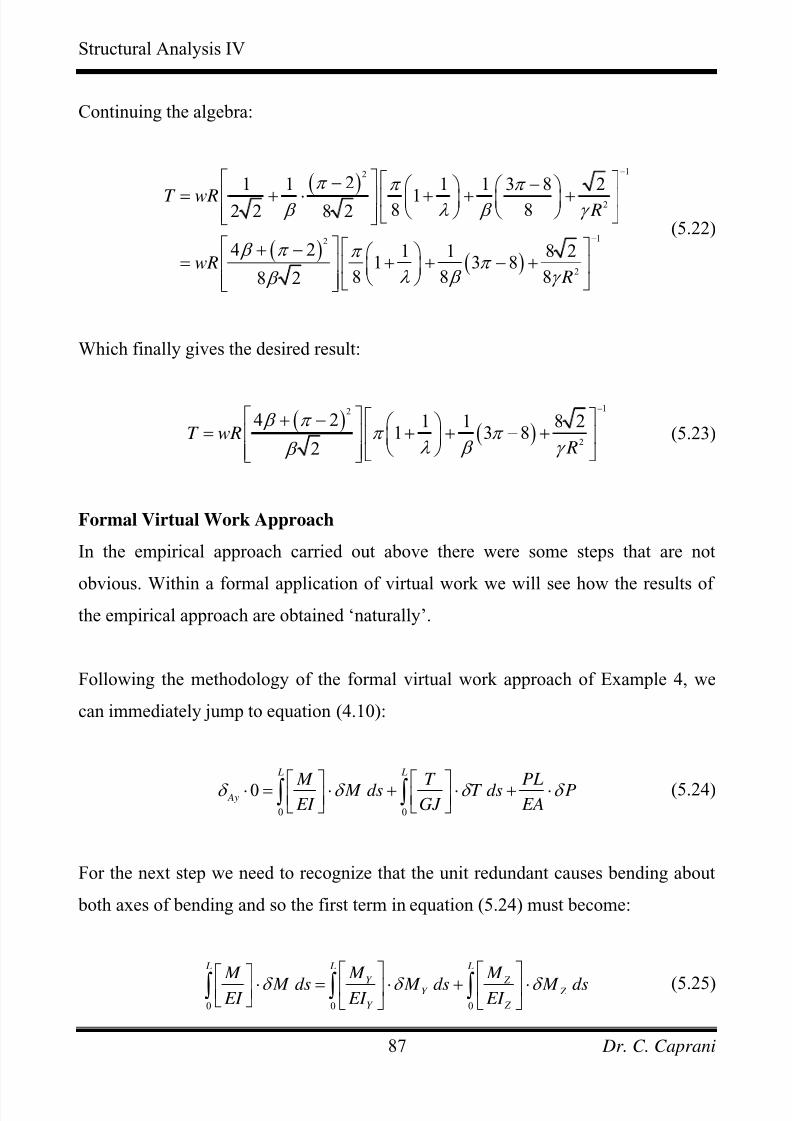
Structural Analysis IV
Formal Virtual Work Approach
Without the use of the insight that equation (4.1) gives, the more formal application
of virtual work will, of course, yield the same result. To calculate the tension in the
cable using virtual work, we use the following:
• Equilibrium system: the external and internal virtual forces corresponding to a
unit virtual force applied in lieu of the redundant;
• Compatible system: the real external and internal displacements of the original
structure subject to the real applied loads.
Thus the virtual work equations are:
0
E I
Ay
W
W W
F M ds T ds e P
δ
δ δ
δ δ κ δ φ δ δ
=
=
⋅ = ⋅ + ⋅ + ⋅∑∫ ∫
(4.9)
In this equation we have accounted for all the major sources of displacement (and
thus virtual work). At this point we acknowledge:
• There is no external virtual force applied, only an internal tension, thus 0F δ = ;
• The real curvatures and twists are expressed using the real bending moments and
torques as M
EI κ = and
T
GJ φ = respectively;
• The elongation of the cable is the only source of axial displacement and is
written in terms of the real tension in the cable, P, as PLe EA
= .
These combine to give, from equation (4.9):
0 0
0
L L
Ay
M T PL M ds T ds P
EI GJ EAδ δ δ
⎡ ⎤ ⎡ ⎤δ ⋅ = ⋅ + ⋅ + ⋅⎢ ⎥ ⎢ ⎥⎣ ⎦ ⎣ ⎦
∫ ∫ (4.10)
As was done in Example 3, using superposition, we write:
Dr. C. Caprani72
7/28/2019 Combined Structures 2009-10
http://slidepdf.com/reader/full/combined-structures-2009-10 73/106
Structural Analysis IV
0 1 0 1 0 1 M M M T T T P P Pα α = + = + = + α (4.11)
However, we know that there is no tension in the cable in the primary structure, since
it is the cable that is the redundant and is thus removed, hence 0 0P = . Using this and
equation (4.11) in equation (4.10) gives:
( ) ( ) ( )0 1 0 1 1
0 0
0
L L M M T T P L M ds T ds P
EI GJ EA
α α α δ δ
⎡ ⎤ ⎡ ⎤+ += ⋅ + ⋅ +⎢ ⎥ ⎢ ⎥
⎢ ⎥ ⎢ ⎥⎣ ⎦ ⎣ ⎦∫ ∫ δ ⋅ (4.12)
Hence:
0 1
0 0
0 1
0 0
1
0
L L
L L
M M M ds M ds
EI EI
T T
T ds T dsGJ GJ
P LP
EA
δ α δ
δ α δ
α δ
= ⋅ + ⋅ ⋅
+ ⋅ + ⋅ ⋅
+ ⋅ ⋅
∫ ∫
∫ ∫(4.13)
And so finally:
0 0
0 0
1 1 1
0 0
L L
L L
M T M ds T ds EI GJ
M T P L M ds T ds P
EI GJ EA
δ δ
α
δ δ δ
⎡ ⎤⋅ + ⋅⎢ ⎥⎣= −
⎡ ⎤⋅ + ⋅ + ⋅⎢ ⎥
⎣ ⎦
∫ ∫
∫ ∫
⎦ (4.14)
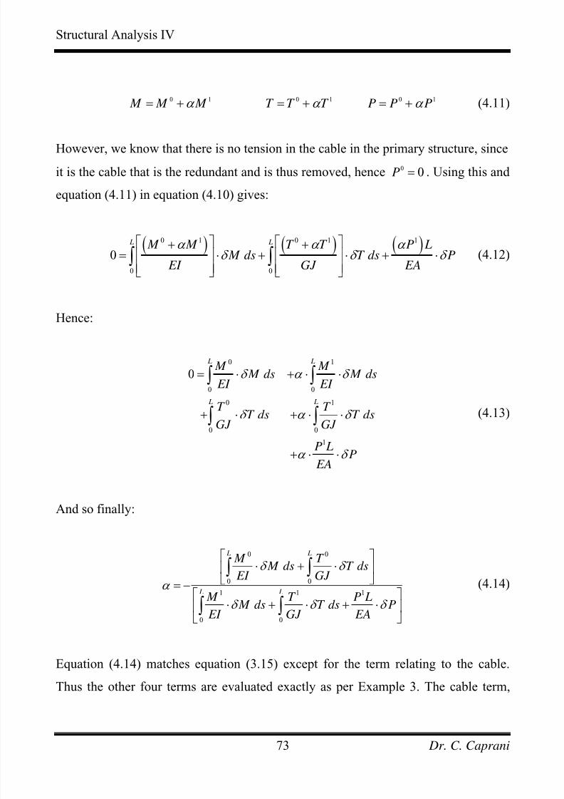
Equation (4.14) matches equation (3.15) except for the term relating to the cable.
Thus the other four terms are evaluated exactly as per Example 3. The cable term,
Dr. C. Caprani73
7/28/2019 Combined Structures 2009-10
http://slidepdf.com/reader/full/combined-structures-2009-10 74/106
Structural Analysis IV
1P L
P EA
δ ⋅ , is easily found once it is recognized that 1 1P Pδ = = as was the case for the
moment and torsion in Example 3. With all the terms thus evaluated, equation (4.14)
becomes the same as equation (4.6) and the solution progresses as before.
The virtual work approach yields the same solution, but without the added insight of
the source of each of the terms in equation (4.14) represented by equation (4.1).
Dr. C. Caprani74
7/28/2019 Combined Structures 2009-10
http://slidepdf.com/reader/full/combined-structures-2009-10 75/106
Structural Analysis IV
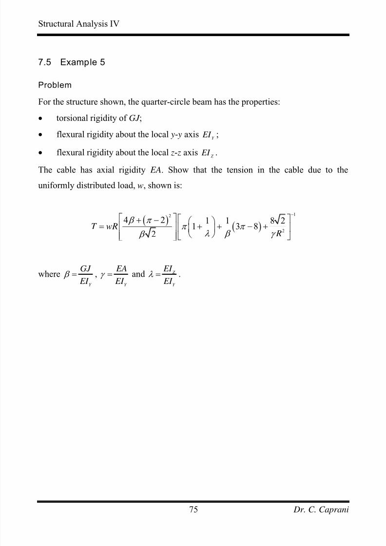
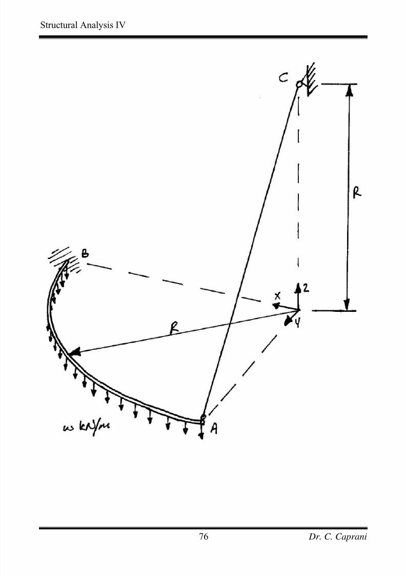
7.5 Example 5
Problem
For the structure shown, the quarter-circle beam has the properties:
• torsional rigidity of GJ ;
• flexural rigidity about the local y- y axisY
EI ;
• flexural rigidity about the local z- z axis Z
EI .
The cable has axial rigidity EA. Show that the tension in the cable due to the
uniformly distributed load, w, shown is:
( )( )
12
2
4 2 1 1 8 21 3 8
2T wR
R
β π π π
λ β γ β
−⎡ ⎤ ⎡ ⎤+ − ⎛ ⎞
= + + −⎢ ⎥ +⎢ ⎥⎜ ⎟⎝ ⎠⎢ ⎥ ⎣ ⎦⎣ ⎦
where
Y
GJ
EI β = ,
Y
EA
EI γ = and Z
Y
EI
EI λ = .
Dr. C. Caprani75
7/28/2019 Combined Structures 2009-10
http://slidepdf.com/reader/full/combined-structures-2009-10 76/106
Structural Analysis IV
Dr. C. Caprani76
7/28/2019 Combined Structures 2009-10
http://slidepdf.com/reader/full/combined-structures-2009-10 77/106
Structural Analysis IV
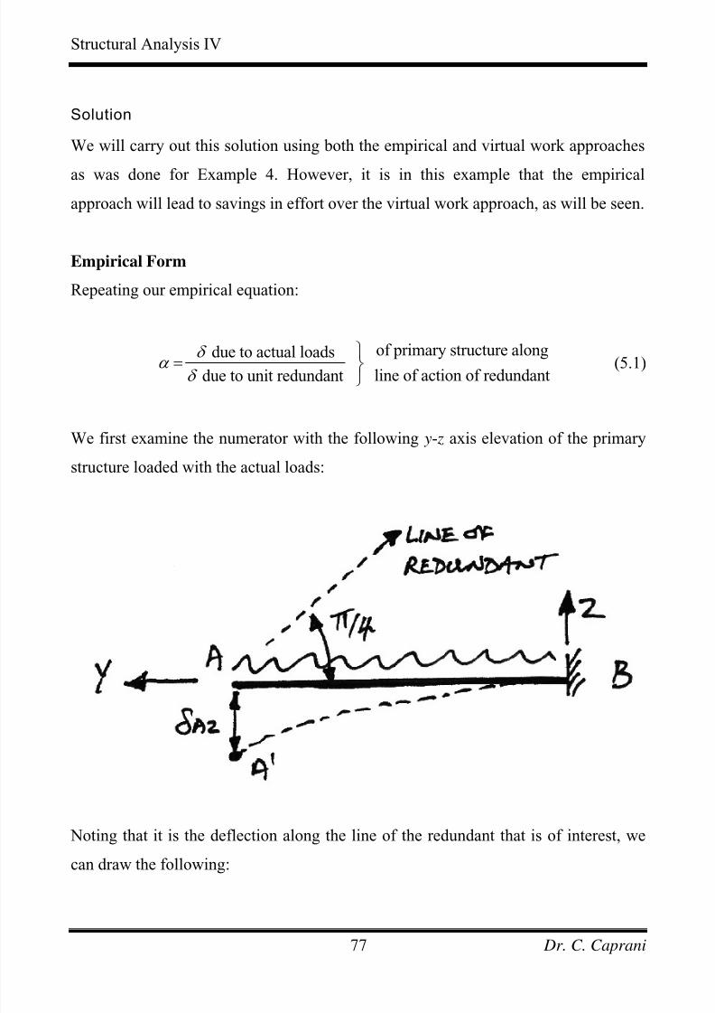
Solution
We will carry out this solution using both the empirical and virtual work approaches
as was done for Example 4. However, it is in this example that the empirical
approach will lead to savings in effort over the virtual work approach, as will be seen.
Empirical Form
Repeating our empirical equation:
of primary structure alongdue to actual loads line of action of redundantdue to unit redundant
δ α δ
⎫= ⎬⎭
(5.1)
We first examine the numerator with the following y- z axis elevation of the primary
structure loaded with the actual loads:
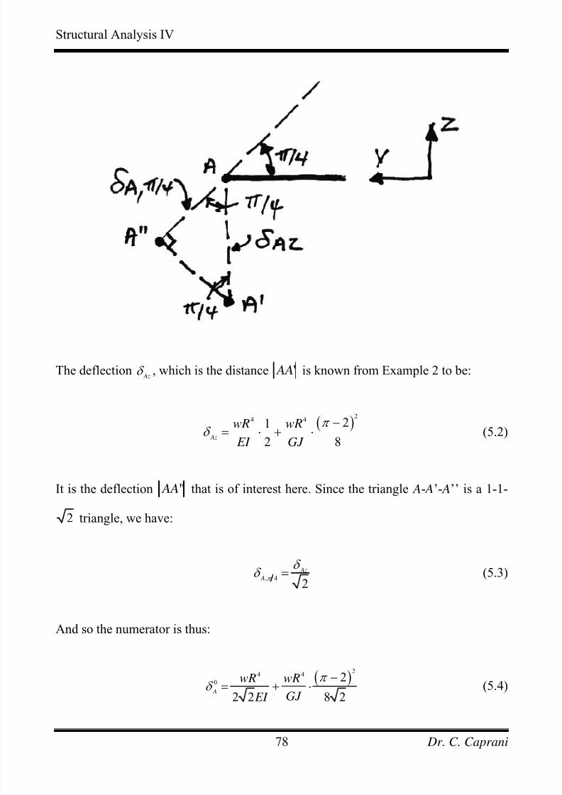
Noting that it is the deflection along the line of the redundant that is of interest, we
can draw the following:
Dr. C. Caprani77
7/28/2019 Combined Structures 2009-10
http://slidepdf.com/reader/full/combined-structures-2009-10 78/106
Structural Analysis IV
The deflection Az
δ , which is the distance ' AA is known from Example 2 to be:
( )24 4 21
2 8 Az
wR wR
EI GJ
π δ −= ⋅ + ⋅ (5.2)
It is the deflection '' AA that is of interest here. Since the triangle A- A’- A’’ is a 1-1-
2 triangle, we have:
, 4
2
Az
A π
δ δ = (5.3)
And so the numerator is thus:
( )2
4 4
02
2 2 8 2 A
wR wR
GJ EI
π δ
−= + ⋅ (5.4)
Dr. C. Caprani78
7/28/2019 Combined Structures 2009-10
http://slidepdf.com/reader/full/combined-structures-2009-10 79/106
Structural Analysis IV
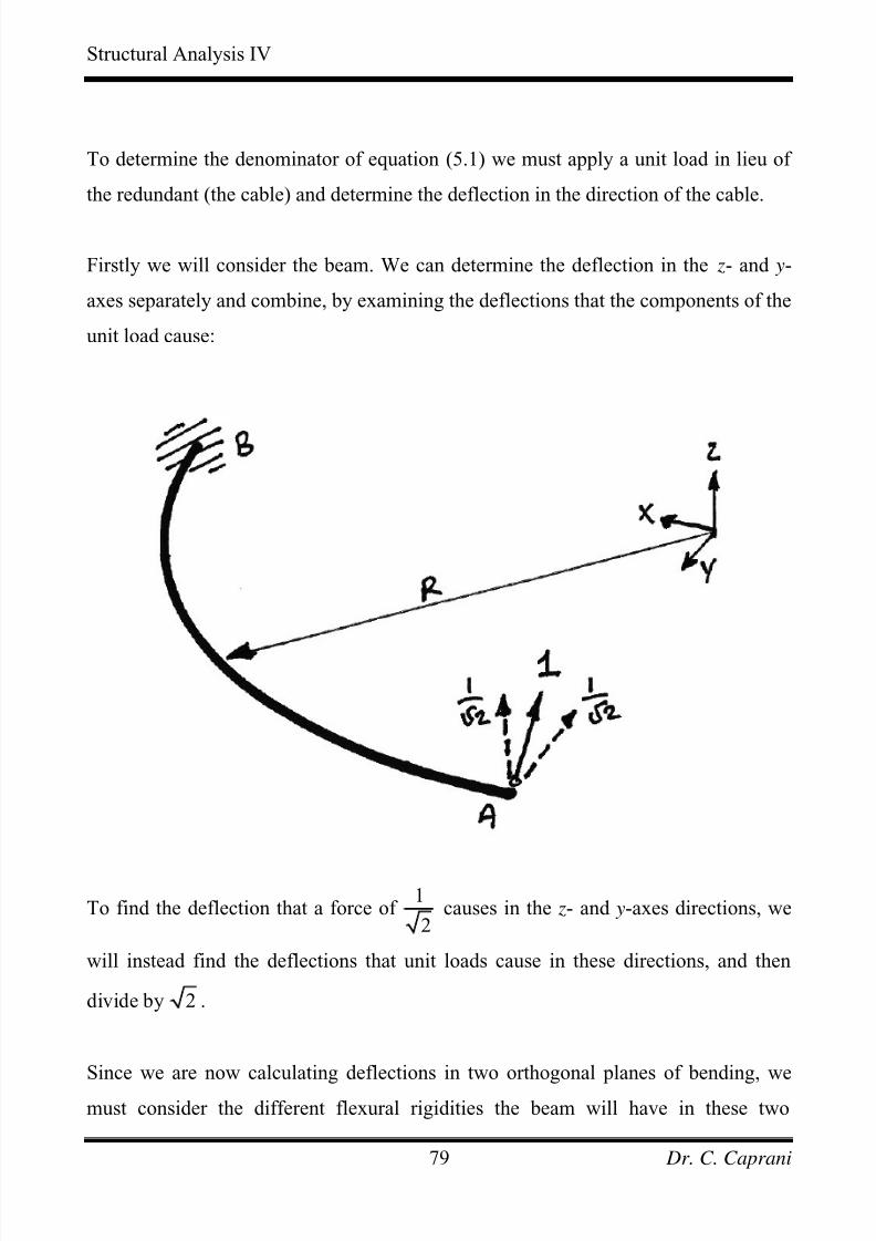
To determine the denominator of equation (5.1) we must apply a unit load in lieu of
the redundant (the cable) and determine the deflection in the direction of the cable.
Firstly we will consider the beam. We can determine the deflection in the z- and y-
axes separately and combine, by examining the deflections that the components of the
unit load cause:
To find the deflection that a force of 1
2causes in the z- and y-axes directions, we
will instead find the deflections that unit loads cause in these directions, and then
divide by 2 .
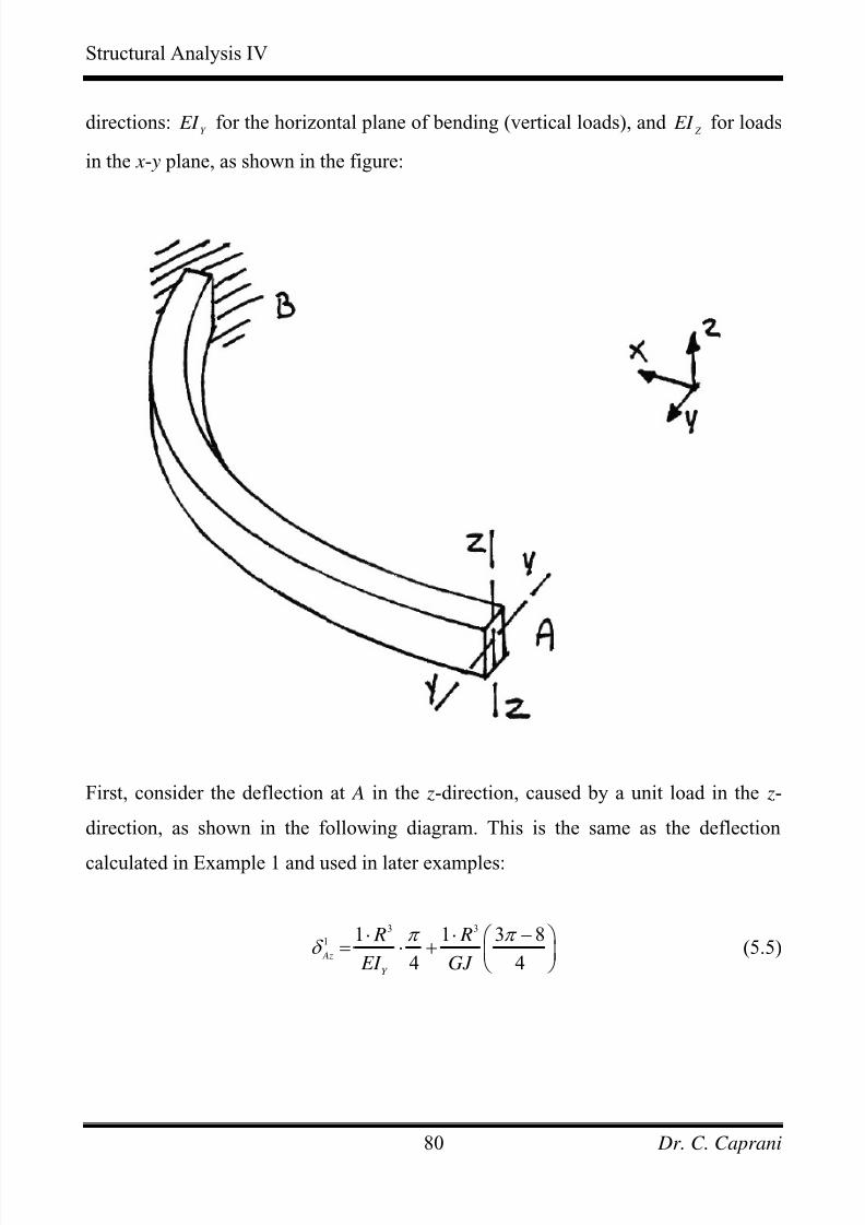
Since we are now calculating deflections in two orthogonal planes of bending, we
must consider the different flexural rigidities the beam will have in these two
Dr. C. Caprani79
7/28/2019 Combined Structures 2009-10
http://slidepdf.com/reader/full/combined-structures-2009-10 80/106
Structural Analysis IV
directions:Y
EI for the horizontal plane of bending (vertical loads), and Z
EI for loads
in the x- y plane, as shown in the figure:
First, consider the deflection at A in the z-direction, caused by a unit load in the z-
direction, as shown in the following diagram. This is the same as the deflection
calculated in Example 1 and used in later examples:
3 3
1 1 1 3
4 4 Az
Y
R R
EI GJ
π π δ
8⋅ ⋅ −⎛ = ⋅ + ⎜
⎝ ⎠
⎞⎟ (5.5)
Dr. C. Caprani80
7/28/2019 Combined Structures 2009-10
http://slidepdf.com/reader/full/combined-structures-2009-10 81/106
Structural Analysis IV
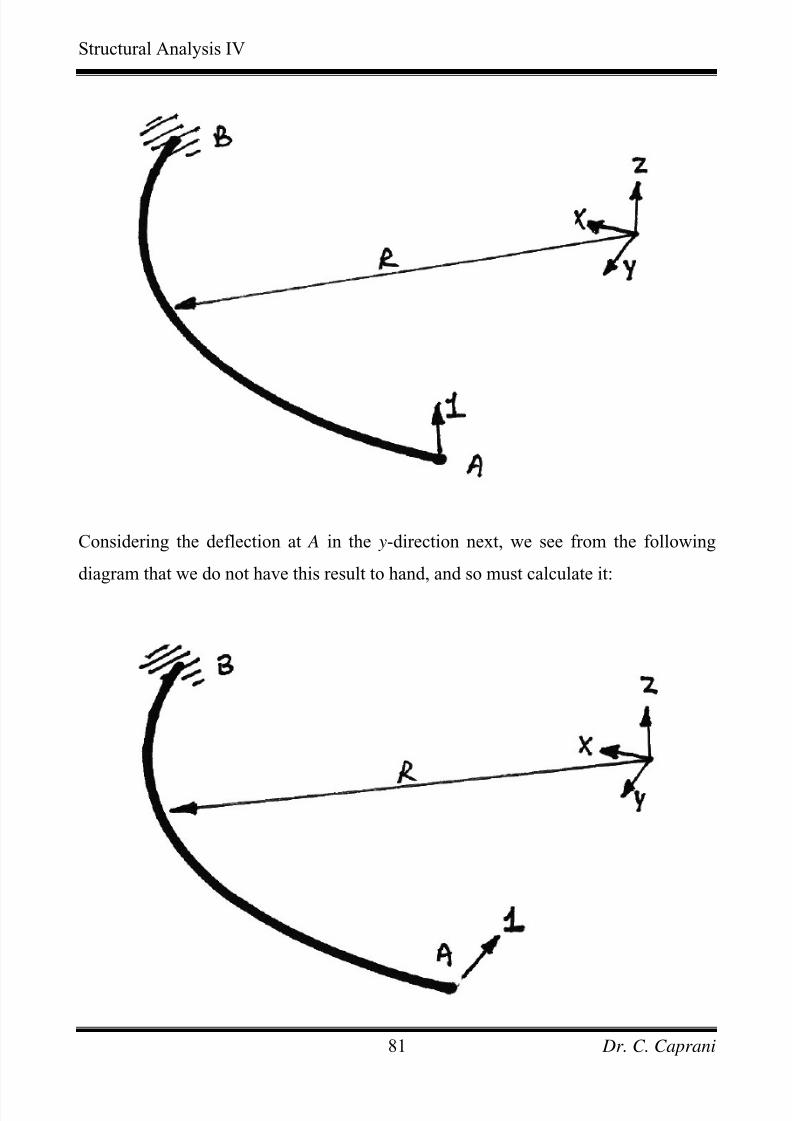
Considering the deflection at A in the y-direction next, we see from the following
diagram that we do not have this result to hand, and so must calculate it:
Dr. C. Caprani81
7/28/2019 Combined Structures 2009-10
http://slidepdf.com/reader/full/combined-structures-2009-10 82/106
Structural Analysis IV
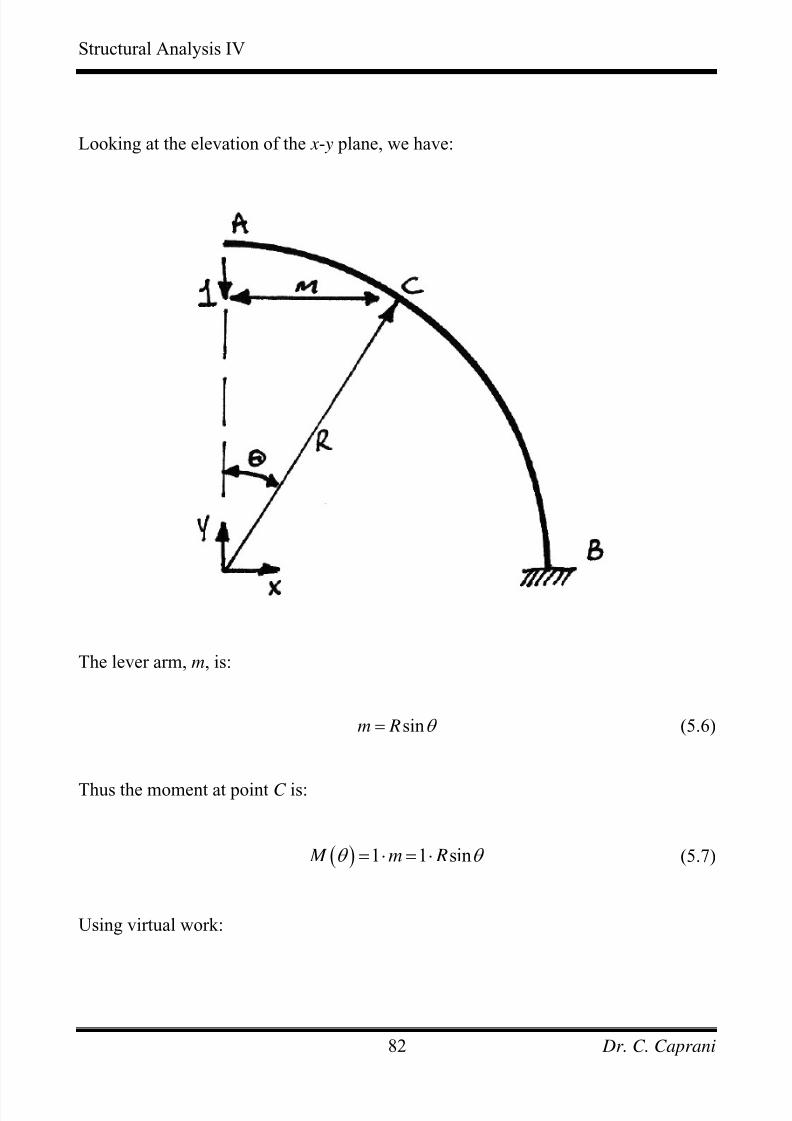
Looking at the elevation of the x- y plane, we have:
The lever arm, m, is:
sinm R θ = (5.6)
Thus the moment at point C is:
( ) 1 1 sin M m Rθ θ = ⋅ = ⋅ (5.7)
Using virtual work:
Dr. C. Caprani82
7/28/2019 Combined Structures 2009-10
http://slidepdf.com/reader/full/combined-structures-2009-10 83/106
Structural Analysis IV
0
1
E I
Ay
W
W W
M ds
δ
δ δ
δ κ δ
=
=
⋅ = ⋅∫
(5.8)
In which we note that there is no torsion term, as the unit load in the x- y plane does
not cause torsion in the structure. Using Z
M EI κ = and ds Rd θ = :
2
0
1 Ay
Z
M M Rd
EI
π
δ δ ⋅ = ∫ θ (5.9)
Since sin M M Rδ θ = = , and assuming the beam is prismatic, we have:
3 2
2
0
1 sin Ay
z
Rd
EI
π
δ θ θ ⋅ = ∫ (5.10)
This is the same as the first term in equation (1.7) and so immediately we obtain the
solution as that of the first term of equation (1.11):
3
1
4 Ay
z
R
EI
π δ = ⋅ (5.11)
In other words, the bending deflection at A in the x- y plane is the same as that in the
z- y plane. This is apparent given that the lever arm is the same in both cases.
However, the overall deflections are not the same due to the presence of torsion in the
z- y plane.
Now that we have the deflections in the two orthogonal planes due to the units loads,
we can determine the deflections in these planes due to the load 12
:
Dr. C. Caprani83
7/28/2019 Combined Structures 2009-10
http://slidepdf.com/reader/full/combined-structures-2009-10 84/106
Structural Analysis IV
3
1 2 1 1 3 8
4 42 Az
Y
R
EI GJ
π π δ
⎡ ⎤−⎛ = ⋅ + ⎜
⎞⎟⎢ ⎥
⎝ ⎠⎣ ⎦(5.12)
3
1 2 1
42 Ay
z
R
EI
π δ
⎡ ⎤= ⋅⎢ ⎥
⎣ ⎦(5.13)
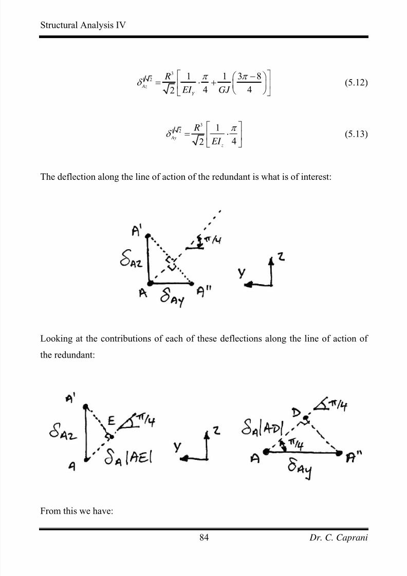
The deflection along the line of action of the redundant is what is of interest:
Looking at the contributions of each of these deflections along the line of action of
the redundant:
From this we have:
Dr. C. Caprani84
7/28/2019 Combined Structures 2009-10
http://slidepdf.com/reader/full/combined-structures-2009-10 85/106
Structural Analysis IV
1 2
3
3
1
2
1 1 1 3
4 42 2
1 1 3 8
2 4 4
Az Az
Y
Y
AE
R
EI GJ
R
EI GJ
δ δ
π π
π π
= ⋅
8⎡ ⎤−⎛ = ⋅ ⋅ + ⎜ ⎞⎟⎢ ⎥⎝ ⎠⎣ ⎦
⎡ ⎤−⎛ ⎞= ⋅ + ⎜ ⎟⎢ ⎥
⎝ ⎠⎣ ⎦
(5.14)
1 2
3
3
1
2
1 1
42 2
1
2 4
Ay Ay
z
z
AD
R
EI
R
EI
δ δ
π
π
=
⎡ ⎤= ⋅ ⋅⎢ ⎥
⎣ ⎦
⎡ ⎤= ⋅⎢ ⎥
⎣ ⎦
(5.15)
Thus the total deflection along the line of action of the redundant is:
1
, 4
3 1 1 3 8 1
2 4 4 2
A Az Ay
Y z
AE AD
R
EI GJ EI
π δ δ δ
3
4
Rπ π
= +
⎡ ⎤−⎛ ⎞= ⋅ + + ⋅⎜ ⎟⎢ ⎥
⎝ ⎠⎣ ⎦
π ⎡ ⎤⎢ ⎥⎣ ⎦
(5.16)
This gives, finally:
3
1
, 4
1 1 1 3 8
2 4 4 A
Y z
R
EI EI GJ π
π π δ
⎡ ⎤⎛ ⎞ −⎛ = + +⎢ ⎜ ⎟ ⎜
⎝ ⎠⎝ ⎠⎣ ⎦
⎞⎥⎟ (5.17)
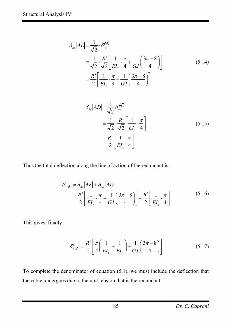
To complete the denominator of equation (5.1), we must include the deflection that
the cable undergoes due to the unit tension that is the redundant:
Dr. C. Caprani85
7/28/2019 Combined Structures 2009-10
http://slidepdf.com/reader/full/combined-structures-2009-10 86/106
Structural Analysis IV
1
2
Le
EA
R
EA
⋅=
=
(5.18)
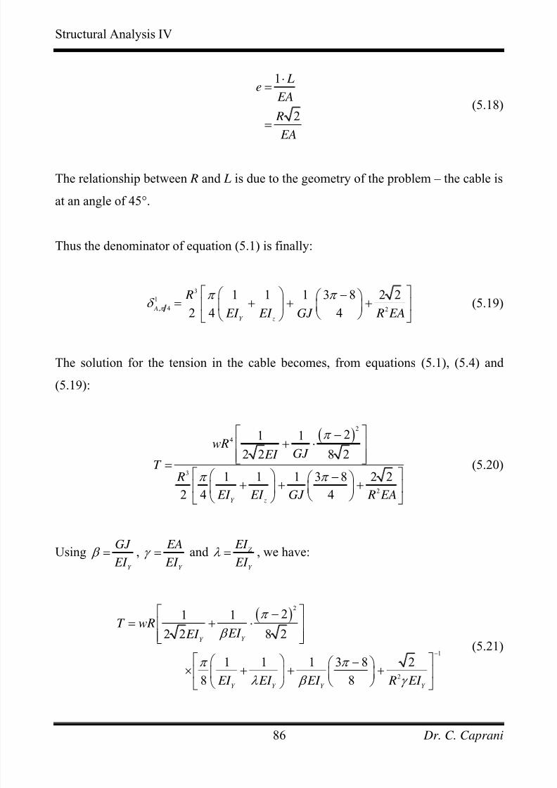
The relationship between R and L is due to the geometry of the problem – the cable is
at an angle of 45°.
Thus the denominator of equation (5.1) is finally:
3
1
, 4 2
1 1 1 3 8 2 2
2 4 4 A
Y z
R
EI EI GJ R EAπ
π π δ
⎡ ⎤⎛ ⎞ −⎛ ⎞= + + +⎢ ⎥⎜ ⎟ ⎜ ⎟
⎝ ⎠⎝ ⎠⎣ ⎦(5.19)
The solution for the tension in the cable becomes, from equations (5.1), (5.4) and
(5.19):
( )2
4
3
2
21 1
2 2 8 2
1 1 1 3 8 2 2
2 4 4Y z
wRGJ EI
T R
EI EI GJ R EA
π
π π
⎡ ⎤−+ ⋅⎢ ⎥
⎢⎣=⎡ ⎤⎛ ⎞ −⎛ ⎞
+ + +⎢ ⎥⎜ ⎟⎜ ⎟⎝ ⎠⎝ ⎠⎣ ⎦
⎥⎦ (5.20)
UsingY
GJ
EI β = ,Y
EA
EI γ = and Z
Y
EI
EI λ = , we have:
( )2
1
2
21 1
2 2 8 2
1 1 1 3 8 2
8 8
Y Y
Y Y Y Y
T wR EI EI
EI EI EI R EI
π
β
π π
λ β γ
−
⎡ ⎤−= + ⋅⎢ ⎥
⎢ ⎥⎣ ⎦
⎡ ⎤⎛ ⎞ −⎛ ⎞× + + +⎢ ⎥⎜ ⎟ ⎜ ⎟
⎝ ⎠⎝ ⎠⎣ ⎦
(5.21)
Dr. C. Caprani86
7/28/2019 Combined Structures 2009-10
http://slidepdf.com/reader/full/combined-structures-2009-10 87/106
Structural Analysis IV
Continuing the algebra:
( )
( )( )
12
2
12
2
21 1 1 1 3 8 218 82 2 8 2
4 2 1 1 8 21 3 8
8 8 88 2
T wR R
wR R
π π π
β λ β
β π π π
λ β γ β
−
−
⎡ ⎤
γ
⎡ ⎤− −⎛ ⎞ ⎛ ⎞= + ⋅ + + +⎢ ⎥ ⎢ ⎥⎜ ⎟ ⎜ ⎟⎝ ⎠ ⎝ ⎠⎢ ⎥ ⎣ ⎦⎣ ⎦
⎡ ⎤ ⎡ ⎤+ − ⎛ ⎞= + + − +⎢ ⎥ ⎢ ⎥⎜ ⎟
⎝ ⎠⎢ ⎥ ⎣ ⎦⎣ ⎦
(5.22)
Which finally gives the desired result:
( )( )
12
2
4 2 1 1 8 21 3 8
2T wR
R
β π π π
λ β γ β
−⎡ ⎤ ⎡ ⎤+ − ⎛ ⎞
= + + −⎢ ⎥ +⎢ ⎥⎜ ⎟⎝ ⎠⎢ ⎥ ⎣ ⎦⎣ ⎦
(5.23)
Formal Virtual Work Approach
In the empirical approach carried out above there were some steps that are not
obvious. Within a formal application of virtual work we will see how the results of the empirical approach are obtained ‘naturally’.
Following the methodology of the formal virtual work approach of Example 4, we
can immediately jump to equation (4.10):
0 0
0
L L
Ay M T PL M ds T ds P EI GJ EA
δ δ δ ⎡ ⎤ ⎡ ⎤ δ ⋅ = ⋅ + ⋅ + ⋅⎢ ⎥ ⎢ ⎥⎣ ⎦ ⎣ ⎦∫ ∫ (5.24)
For the next step we need to recognize that the unit redundant causes bending about
both axes of bending and so the first term in equation (5.24) must become:
0 0 0
L L L
Y Z Y
Y Z
M M M Z M ds M ds M ds
EI EI EI δ δ
⎡ ⎤ ⎡ ⎤⎡ ⎤⋅ = ⋅ + ⋅⎢ ⎥ ⎢ ⎥⎢ ⎥⎣ ⎦ ⎣ ⎦ ⎣ ⎦∫ ∫ ∫ δ (5.25)
Dr. C. Caprani87
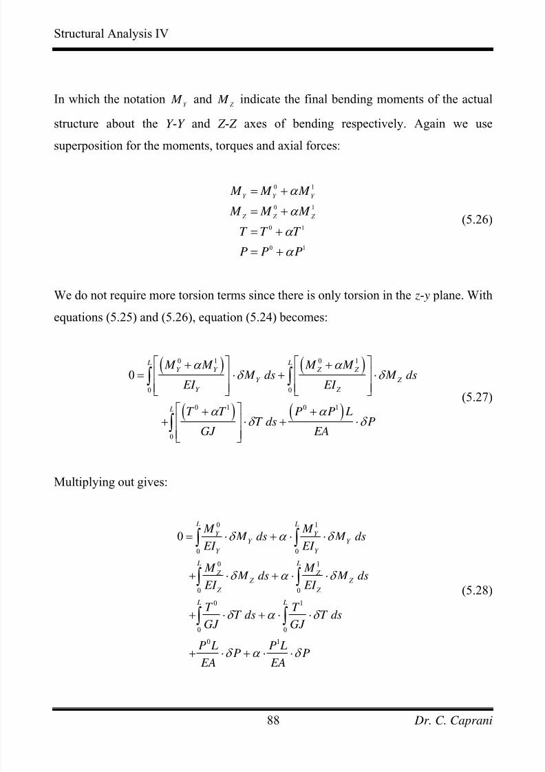
7/28/2019 Combined Structures 2009-10
http://slidepdf.com/reader/full/combined-structures-2009-10 88/106
Structural Analysis IV
In which the notationY
M and Z
M indicate the final bending moments of the actual
structure about the Y -Y and Z - Z axes of bending respectively. Again we use
superposition for the moments, torques and axial forces:
0 1
0 1
0 1
0 1
Y Y Y
Z Z Z
M M M
M M M
T T T
P P P
α
α
α
α
= +
= +
= +
= +
(5.26)
We do not require more torsion terms since there is only torsion in the z- y plane. With
equations (5.25) and (5.26), equation (5.24) becomes:
( ) ( )
( ) ( )
0 1 0 1
0 0
0 1 0 1
0
0 L L
Y Y Z Z
Y Z
Y Z
L
M M M M M ds M ds
EI EI
T T P P LT ds P
GJ EA
α α δ δ
α α δ δ
⎡ ⎤ ⎡ ⎤+ += ⋅ + ⋅⎢ ⎥ ⎢ ⎥
⎢ ⎥ ⎢ ⎥⎣ ⎦ ⎣ ⎦
⎡ ⎤+ ++ ⋅ + ⋅⎢ ⎥
⎢ ⎥⎣ ⎦
∫ ∫
∫
(5.27)
Multiplying out gives:
0 1
0 0
0 1
0 0
0 1
0 0
0 1
0
L L
Y Y
Y Y Y Y
L L
Z Z Z Z
Z Z
L L
M M
M ds M ds EI EI
M M M ds M ds
EI EI
T T T ds T ds
GJ GJ
P L P LP P
EA EA
δ α δ
δ α δ
δ α δ
δ α δ
= ⋅ + ⋅ ⋅
+ ⋅ + ⋅ ⋅
+ ⋅ + ⋅ ⋅
+ ⋅ + ⋅ ⋅
∫ ∫
∫ ∫
∫ ∫
(5.28)
Dr. C. Caprani88
7/28/2019 Combined Structures 2009-10
http://slidepdf.com/reader/full/combined-structures-2009-10 89/106
Structural Analysis IV
At this point we recognize that some of the terms are zero:
• There is no axial force in the primary structure since the cable is ‘cut’, and so
0 0P = ;
• There is no bending in the x- y plane (about the z- z axis of the beam) in the
primary structure as the loading is purely vertical, thus 0 0 Z
M = .
Including these points, and solving for α gives:
0 0
0 0
1 1 1 1
0 0 0
L L
Y Y
Y
L L L
Y Z Y Z
Y Z
M T M ds T ds
EI GJ
M M T P L M ds M ds T ds P
EI EI GJ EA
δ δ
α δ δ δ
⎡ ⎤⋅ + ⋅⎢ ⎥
⎣ ⎦
= − ⎡ ⎤⋅ + ⋅ + ⋅ + ⋅⎢ ⎥
⎣ ⎦
∫ ∫
∫ ∫ ∫ δ (5.29)
We will next examine this expression term-by-term.
0
0
L
Y
Y Y
M M ds
EI δ ⋅
∫
For this term, 0
Y M are the moments caused by the UDL about the y- y axis of bending,
as per equation (2.2):
( ) ( )0 2 1 cosY
M wRθ θ = − (5.30)
Y M δ are the moments about the same axis caused by the unit redundant. Since this
redundant acts at an angle of 45° to the plane of interest, these moments are caused
by its vertical component of 1
2. From equation (1.4), we thus have:
( )1
sin2Y M Rδ θ = − θ (5.31)
Dr. C. Caprani89
7/28/2019 Combined Structures 2009-10
http://slidepdf.com/reader/full/combined-structures-2009-10 90/106
Structural Analysis IV
Notice that we have taken it that downwards loading causes positive bending
moments. Thus we have:
( )
( )
02
0 0
23
0
1 11 cos sin
2
sin sin cos2
L L
Y Y
Y Y
Y
M M ds wR R ds
EI EI
wR Rd
EI
π
δ θ
θ θ θ θ
θ ⎡ ⎤
⎡ ⎤⋅ = − −⎢ ⎥⎣ ⎦⎣ ⎦
= − −
∫ ∫
∫
(5.32)
In which we have used the relation ds Rd θ = . From the integral appendix we thus
have:
[ ]
( ) ( ) ( ) ( )
20 42
000
3
1cos cos2
42
10 1 1 1
42
L
Y Y
Y Y
Y
M wR M ds
EI EI
wR
EI
π π
δ θ θ ⎧ ⎫⎪ ⎪⎡ ⎤
⋅ = − − − −⎨ ⎬⎢ ⎥⎣ ⎦⎪ ⎪⎩ ⎭
⎧ ⎫= − − − + − −⎡ ⎤ ⎡ ⎤⎨ ⎬⎣ ⎦ ⎣ ⎦
⎩ ⎭
∫(5.33)
And so finally:
0 4
0 2 2
L
Y Y
Y Y
M wR M ds
EI EI δ ⋅ = −∫ (5.34)
0
0
LT
T dsGJ
δ ⋅∫
The torsion caused by the UDL in the primary structure is the same as that from
equation (2.3):
( ) ( )0 2 sinT wRθ θ θ = − (5.35)
Dr. C. Caprani90
7/28/2019 Combined Structures 2009-10
http://slidepdf.com/reader/full/combined-structures-2009-10 91/106
Structural Analysis IV
Similarly to the bending term, the torsion caused by the unit redundant is1
2that of
the unit load of equation (2.6):
( ) (1
1 cos2
T R )δ θ = − − θ (5.36)
Again note that we take the downwards loads as causing positive torsion. Noting
ds Rd θ = we thus have:
( ) ( )
( )( )
202
0 0
24
0
1 1sin 1 cos
2
sin 1 cos2
LT
T ds wR R Rd GJ GJ
wRd
GJ
π
π
δ θ θ θ
θ θ θ θ
⎡ ⎤⎡ ⎤⋅ = − − −⎢ ⎥⎣ ⎦
⎣
= − − −
∫ ∫
∫
θ ⎦
(5.37)
This integral is exactly that of the second term in equation (2.8). Hence we can take
its result from equation (2.9) to give:
( )2
20 4
0
2
82
LT wR
T dsGJ GJ
π δ
−⋅ = − ⋅∫ (5.38)
1
0
L
Y Y
Y
M M ds
EI δ ⋅∫
Dr. C. Caprani91
7/28/2019 Combined Structures 2009-10
http://slidepdf.com/reader/full/combined-structures-2009-10 92/106
Structural Analysis IV
For this term we recognize that 1
Y Y M M δ = and are the moments caused by the
1
2
component of the unit redundant in the vertical direction and are thus given by
equation (1.1):
( )1 1sin
2Y Y
M M Rδ θ = = θ (5.39)
Hence this term becomes:
1 2
0 0
3 2
2
0
1 1 1sin sin
2 2
sin2
L
Y
Y
Y Y
Y
M M ds R R Rd
EI EI
Rd
EI
π
π
δ θ θ
θ θ
⎡ ⎤ ⎡ ⎤⋅ = ⎢ ⎥ ⎢ ⎥
⎣ ⎦ ⎣ ⎦
=
∫ ∫
∫
θ
(5.40)
From the integral tables we thus have:
( )
21 3
0 0
3
1sin2
2 2 4
10 0 0
2 4 4
L
Y
Y
Y Y
Y
M R M ds
EI EI
R
EI
π
θ δ θ
π
⎡ ⎤⋅ = −⎢ ⎥⎣ ⎦
⎡ ⎤⎛ ⎞= − ⋅ − −⎜ ⎟⎢ ⎥
⎝ ⎠⎣ ⎦
∫(5.41)
And so we finally have:
1 3
0 8
L
Y
Y
Y Y
M M ds
EI EI
R π δ ⋅ = ⋅∫ (5.42)
1
0
L
Z
Z Z
M M ds
EI δ ⋅
∫
Dr. C. Caprani92
7/28/2019 Combined Structures 2009-10
http://slidepdf.com/reader/full/combined-structures-2009-10 93/106
Structural Analysis IV
Again we recognize that 1
Z Z M M δ = and are the moments caused by the
1
2
component of the unit redundant in the x- y plane and are thus given by equation (5.7).
Hence this term becomes:
1 2
0 0
1 1 1sin sin
2 2
L
Y
Y
Y Y
M M ds R R Rd
EI EI
π
δ θ θ ⎡ ⎤ ⎡ ⎤
⋅ = ⎢ ⎥ ⎢ ⎥⎣ ⎦ ⎣ ⎦
∫ ∫ θ (5.43)
This is the same as equation (5.40) except for the different flexural rigidity, and so
the solution is got from equation (5.42) to be:
1 3
0 8
L
Z
Z
Z Z
M M ds
EI EI
R π δ ⋅ = ⋅∫ (5.44)
1
0
LT
T ds
GJ
δ ⋅∫
Once again note that 1T T δ = and are the torques caused by the1
2vertical
component of the unit redundant. From equation (1.2), then we have:
(1 11 cos
2
T T R )δ θ = = − (5.45)
Thus:
( ) ( )
( )
21
0 0
232
0
1 1 11 cos 1 cos
2 2
1 cos2
LT
T ds R R Rd GJ GJ
R
d GJ
π
π
δ θ θ
θ θ
⎡ ⎤ ⎡ ⎤⋅ = − −⎢ ⎥ ⎢ ⎥
⎣ ⎦ ⎣
= −
∫ ∫
∫
θ ⎦ (5.46)
Dr. C. Caprani93
7/28/2019 Combined Structures 2009-10
http://slidepdf.com/reader/full/combined-structures-2009-10 94/106
Structural Analysis IV
This integral is that of equation (1.9) and so the solution is:
1 3
0
3 8
8
LT R
T dsGJ GJ
π δ
−⎛ ⋅ = ⎜
⎝ ⎠∫
⎞⎟ (5.47)
1P L
P EA
δ ⋅
Lastly then, since 1 1P Pδ = = and 2 L R= , this term is easily calculated to be:
12P L R
P EA E
δ ⋅ = A
(5.48)
With the values for all terms now worked out, we substitute these values into
equation (5.29) to determine the cable tension:
( )2
24 4
3 3 3
2
82 2 2
3 8 2
8 8 8
Y
Y Z
wR wR
EI GJ
R R R R
EI EI GJ EA
π
α π π π
⎡ ⎤−⎢ ⎥− − ⋅⎢ ⎥⎣= −
⎡ ⎤−⎛ ⎞⋅ + ⋅ + +⎢ ⎥⎜ ⎟
⎝ ⎠⎣ ⎦
⎦ (5.49)
Cancelling the negatives and re-arranging gives:
( )2
4
3
2
21 1
2 2 8 2
1 1 1 3 8 2 2
2 4 4
Y
Y z
wRGJ EI
T R
EI EI GJ R EA
π
π π
⎡ ⎤−+ ⋅⎢ ⎥
⎢⎣=⎡ ⎤⎛ ⎞ −⎛ ⎞
+ + +⎢ ⎥⎜ ⎟⎜ ⎟⎝ ⎠⎝ ⎠⎣ ⎦
⎥⎦ (5.50)
Dr. C. Caprani94
7/28/2019 Combined Structures 2009-10
http://slidepdf.com/reader/full/combined-structures-2009-10 95/106
Structural Analysis IV
And this is the same as equation (5.20) and so the solution can proceed as before to
obtain the tension in the cable as per equation (5.23).
Comparison of the virtual work with the empirical form illustrates the interpretation
of each of the terms in the virtual work equation that is inherent in the empirical view
of such problems.
Dr. C. Caprani95
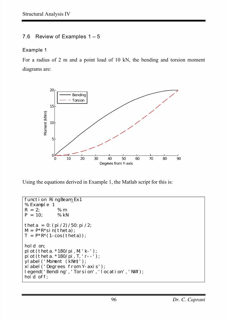
7/28/2019 Combined Structures 2009-10
http://slidepdf.com/reader/full/combined-structures-2009-10 96/106
Structural Analysis IV
7.6 Review of Examples 1 – 5
Example 1
For a radius of 2 m and a point load of 10 kN, the bending and torsion moment
diagrams are:
0 10 20 30 40 50 60 70 80 900
5
10
15
20
M o m e n t ( k N m )
Degrees from Y-axis
Bending
Torsion
Using the equations derived in Example 1, the Matlab script for this is:
f unct i on Ri ngBeam_Ex1% Exampl e 1R = 2; % mP = 10; % kN
t het a = 0: ( pi / 2) / 50: pi / 2;M = P*R*si n( t het a) ;
T = P*R*( 1- cos( t heta) ) ;
hol d on;pl ot ( t het a. *180/ pi , M, ' k- ' ) ;pl ot ( t het a. *180/ pi , T, ' r - - ' ) ;yl abel ( ' Moment ( kNm) ' ) ;xl abel ( ' Degr ees f r om Y- axi s ' ) ;l egend( ' Bendi ng' , ' Tor si on' , ' l ocat i on' , ' NW' ) ;hol d of f ;
Dr. C. Caprani96
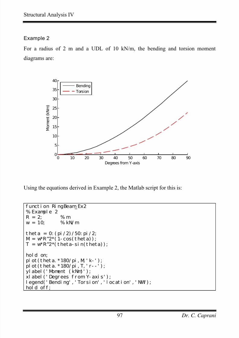
7/28/2019 Combined Structures 2009-10
http://slidepdf.com/reader/full/combined-structures-2009-10 97/106
Structural Analysis IV
Example 2
For a radius of 2 m and a UDL of 10 kN/m, the bending and torsion moment
diagrams are:
0 10 20 30 40 50 60 70 80 900
5
10
15
20
25
30
35
40
M o m e n t ( k N m )
Degrees from Y-axis
Bending
Torsion
Using the equations derived in Example 2, the Matlab script for this is:
f unct i on Ri ngBeam_Ex2% Exampl e 2R = 2; % mw = 10; % kN/ m t het a = 0: ( pi / 2) / 50: pi / 2;M = w*R 2̂*( 1- cos( t het a) ) ;
T = w*R 2̂*( t heta- si n( t heta) ) ;
hol d on;pl ot ( t het a. *180/ pi , M, ' k- ' ) ;pl ot ( t het a. *180/ pi , T, ' r - - ' ) ;yl abel ( ' Moment ( kNm) ' ) ;xl abel ( ' Degr ees f r om Y- axi s ' ) ;l egend( ' Bendi ng' , ' Tor si on' , ' l ocat i on' , ' NW' ) ;hol d of f ;
Dr. C. Caprani97
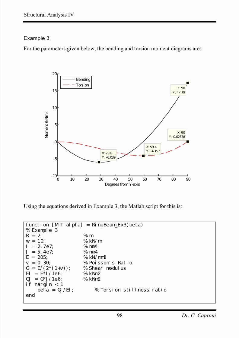
7/28/2019 Combined Structures 2009-10
http://slidepdf.com/reader/full/combined-structures-2009-10 98/106
Structural Analysis IV
Example 3
For the parameters given below, the bending and torsion moment diagrams are:
0 10 20 30 40 50 60 70 80 90-10
-5
0
5
10
15
20
X: 90
Y: 17.19
X: 59.4
Y: -4.157
X: 90
Y: 0.02678 M o m e n t ( k N
m )
Degrees from Y-axis
X: 28.8
Y: -6.039
Bending
Torsion
Using the equations derived in Example 3, the Matlab script for this is:
f unct i on [ M T al pha] = Ri ngBeam_Ex3( beta)% Exampl e 3
R = 2; % mw = 10; % kN/ mI = 2. 7e7; % mm4
J = 5. 4e7; % mm4E = 205; % kN/ mm2v = 0. 30; % Poi sson' s Rat i oG = E/ ( 2*( 1+v) ) ; % Shear modul usEI = E*I / 1e6; % kNm2GJ = G*J / 1e6; % kNm2i f nar gi n < 1
bet a = GJ / EI ; % Tor si on st i f f ness r at i o
end
Dr. C. Caprani98
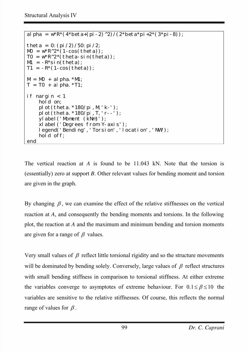
7/28/2019 Combined Structures 2009-10
http://slidepdf.com/reader/full/combined-structures-2009-10 99/106
Structural Analysis IV
al pha = w*R*( 4*bet a+( pi - 2) 2̂) / ( 2*bet a*pi +2*( 3*pi - 8) ) ;
t het a = 0: ( pi / 2) / 50: pi / 2;M0 = w*R 2̂*( 1- cos( t het a) ) ;
T0 = w*R 2̂*( t heta- si n( t heta) ) ;
M1 = - R*s i n( t het a) ; T1 = - R*( 1- cos( t heta) ) ;
M = M0 + al pha. *M1; T = T0 + al pha. *T1;
i f nar gi n < 1hol d on;pl ot ( t het a. *180/ pi , M, ' k- ' ) ;pl ot ( thet a. *180/ pi , T, ' r - - ' ) ;yl abel ( ' Moment ( kNm) ' ) ;
xl abel ( ' Degr ees f r om Y- axi s ' ) ;l egend( ' Bendi ng' , ' Tor si on' , ' l ocat i on' , ' NW' ) ;hol d of f ;
end
The vertical reaction at A is found to be 11.043 kN. Note that the torsion is
(essentially) zero at support B. Other relevant values for bending moment and torsion
are given in the graph.
By changing β , we can examine the effect of the relative stiffnesses on the vertical
reaction at A, and consequently the bending moments and torsions. In the following
plot, the reaction at A and the maximum and minimum bending and torsion moments
are given for a range of β values.
Very small values of β reflect little torsional rigidity and so the structure movements
will be dominated by bending solely. Conversely, large values of β reflect structures
with small bending stiffness in comparison to torsional stiffness. At either extreme
the variables converge to asymptotes of extreme behaviour. For 0.1 10 β ≤ ≤ the
variables are sensitive to the relative stiffnesses. Of course, this reflects the normal
range of values for β .
Dr. C. Caprani99
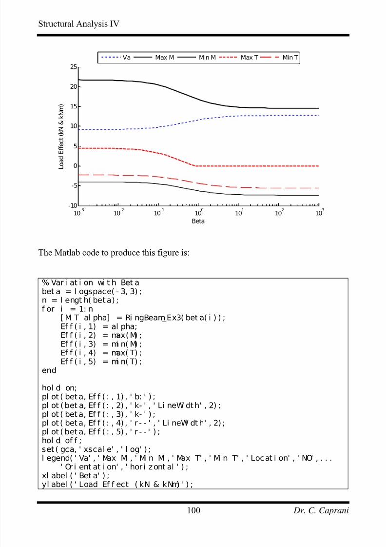
7/28/2019 Combined Structures 2009-10
http://slidepdf.com/reader/full/combined-structures-2009-10 100/106
Structural Analysis IV
10-3
10-2
10-1
100
101
102
103
-10
-5
0
5
10
15
20
25
Beta
L o a d E f f e c t ( k N & k N m )
Va Max M Min M Max T Min T
The Matlab code to produce this figure is:
% Var i at i on wi t h Bet abet a = l ogspace( - 3, 3) ;n = l engt h( beta) ;f or i = 1: n
[ M T al pha] = Ri ngBeam_Ex3( bet a( i ) ) ;Ef f ( i , 1) = al pha;Ef f ( i , 2) = max(M) ;Ef f ( i , 3) = mi n( M) ;Ef f ( i , 4) = max( T) ;Ef f ( i , 5) = mi n( T) ;
end
hol d on;pl ot ( bet a, Ef f ( : , 1) , ' b: ' ) ;pl ot (bet a, Ef f ( : , 2) , ' k- ' , ' Li neWi dth' , 2) ;pl ot ( bet a, Ef f ( : , 3) , ' k- ' ) ;pl ot ( beta, Ef f ( : , 4) , ' r - - ' , ' Li neWi dth' , 2) ;pl ot ( bet a, Ef f ( : , 5) , ' r - - ' ) ;hol d of f ;set ( gca, ' xscal e' , ' l og' ) ;l egend( ' Va' , ' Max M' , ' Mi n M' , ' Max T' , ' Mi n T' , ' Locat i on' , ' NO' , . . .
' Or i ent at i on' , ' hor i zont al ' ) ;
xl abel ( ' Bet a' ) ;yl abel ( ' Load Ef f ect ( kN & kNm) ' ) ;
Dr. C. Caprani100
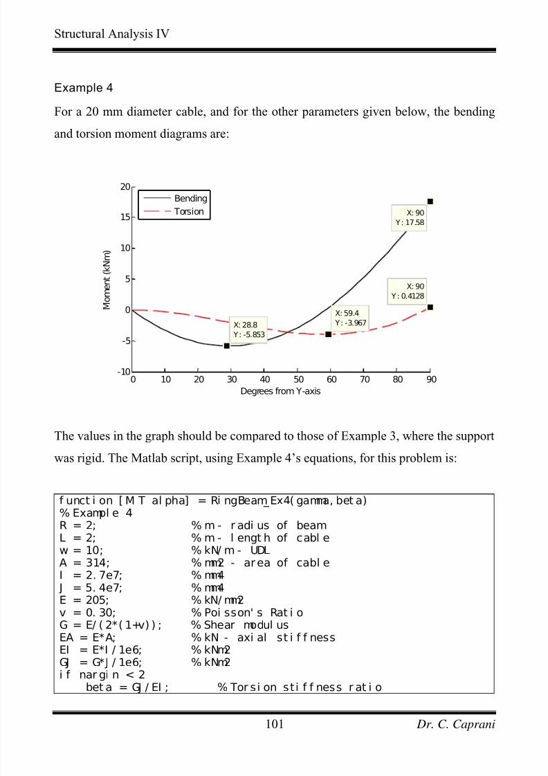
7/28/2019 Combined Structures 2009-10
http://slidepdf.com/reader/full/combined-structures-2009-10 101/106
Structural Analysis IV
Example 4
For a 20 mm diameter cable, and for the other parameters given below, the bending
and torsion moment diagrams are:
0 10 20 30 40 50 60 70 80 90-10
-5
0
5
10
15
20
X: 90
Y: 17.58
X: 59.4
Y: -3.967X: 28.8
Y: -5.853
X: 90
Y: 0.4128
M o m e n t ( k N m )
Degrees from Y-axis
Bending
Torsion
The values in the graph should be compared to those of Example 3, where the support
was rigid. The Matlab script, using Example 4’s equations, for this problem is:
f unct i on [ M T al pha] = Ri ngBeam_Ex4( gamma, bet a)% Exampl e 4R = 2; % m - r adi us of beam
L = 2; % m - l engt h of cabl ew = 10; % kN/ m - UDLA = 314; % mm2 - ar ea of cabl eI = 2. 7e7; % mm4
J = 5. 4e7; % mm4E = 205; % kN/ mm2v = 0. 30; % Poi sson' s Rat i oG = E/ ( 2*( 1+v) ) ; % Shear modul usEA = E*A; % kN - axi al st i f f nessEI = E*I / 1e6; % kNm2GJ = G*J / 1e6; % kNm2
i f nar gi n < 2bet a = GJ / EI ; % Tor si on st i f f ness r at i o
Dr. C. Caprani101
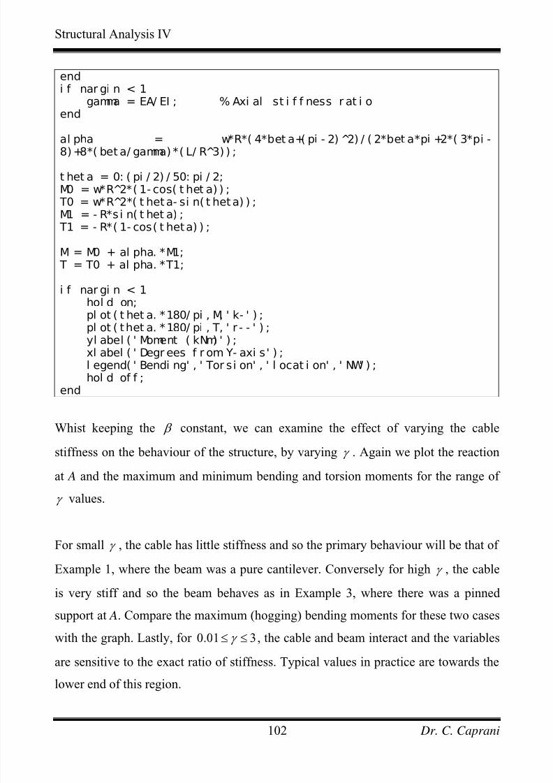
7/28/2019 Combined Structures 2009-10
http://slidepdf.com/reader/full/combined-structures-2009-10 102/106
Structural Analysis IV
endi f nar gi n < 1
gamma = EA/ EI ; % Axi al st i f f ness r at i oend
al pha = w*R*( 4*bet a+( pi - 2) 2̂) / ( 2*bet a*pi +2*( 3*pi -8)+8*( bet a/ gamma) *( L/ R 3̂) ) ;
t het a = 0: ( pi / 2) / 50: pi / 2;M0 = w*R 2̂*( 1- cos( t het a) ) ;
T0 = w*R 2̂*( t heta- si n( t heta) ) ;M1 = - R*s i n( t het a) ;
T1 = - R*( 1- cos( t heta) ) ;
M = M0 + al pha. *M1; T = T0 + al pha. *T1;
i f nar gi n < 1hol d on;pl ot ( t het a. *180/ pi , M, ' k- ' ) ;pl ot ( thet a. *180/ pi , T, ' r - - ' ) ;yl abel ( ' Moment ( kNm) ' ) ;xl abel ( ' Degr ees f r om Y- axi s ' ) ;l egend( ' Bendi ng' , ' Tor si on' , ' l ocat i on' , ' NW' ) ;hol d of f ;
end
Whist keeping the β constant, we can examine the effect of varying the cable
stiffness on the behaviour of the structure, by varying γ . Again we plot the reaction
at A and the maximum and minimum bending and torsion moments for the range of
γ values.
For small γ , the cable has little stiffness and so the primary behaviour will be that of
Example 1, where the beam was a pure cantilever. Conversely for high γ , the cable
is very stiff and so the beam behaves as in Example 3, where there was a pinned
support at A. Compare the maximum (hogging) bending moments for these two cases
with the graph. Lastly, for 0.01 3γ ≤ ≤ , the cable and beam interact and the variables
are sensitive to the exact ratio of stiffness. Typical values in practice are towards the
lower end of this region.
Dr. C. Caprani102
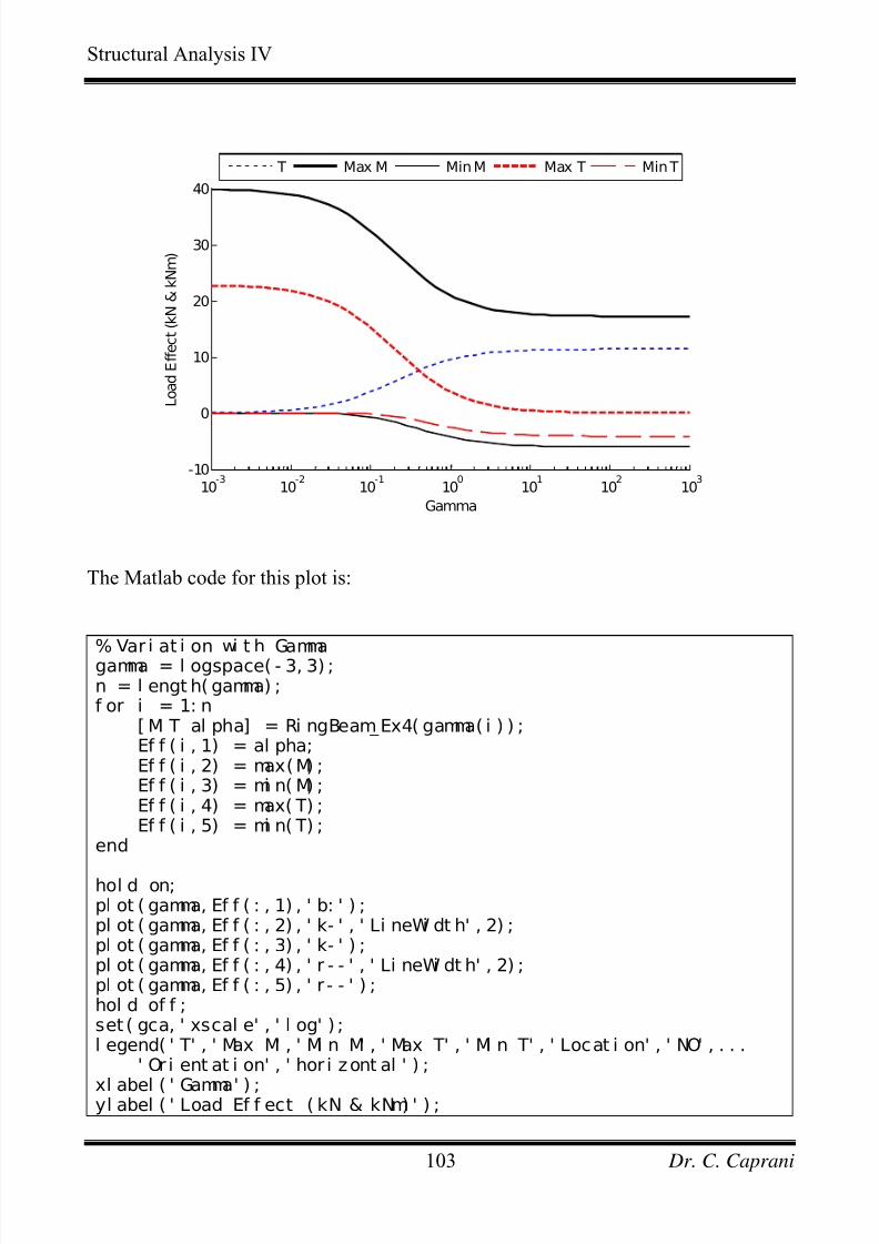
7/28/2019 Combined Structures 2009-10
http://slidepdf.com/reader/full/combined-structures-2009-10 103/106
Structural Analysis IV
10-3
10-2
10-1
100
101
102
103
-10
0
10
20
30
40
Gamma
L o a d E f f e c t ( k N & k N m )
T Max M Min M Max T Min T
The Matlab code for this plot is:
% Var i at i on wi t h Gammagamma = l ogspace( - 3, 3) ;n = l engt h( gamma) ;f or i = 1: n
[ M T al pha] = Ri ngBeam_Ex4( gamma( i ) ) ;Ef f ( i , 1) = al pha;Ef f ( i , 2) = max(M) ;Ef f ( i , 3) = mi n( M) ;Ef f ( i , 4) = max( T) ;Ef f ( i , 5) = mi n( T) ;
end
hol d on;pl ot ( gamma, Ef f ( : , 1) , ' b: ' ) ;pl ot ( gamma, Ef f ( : , 2) , ' k- ' , ' Li neWi dt h' , 2) ;pl ot ( gamma, Ef f ( : , 3) , ' k- ' ) ;pl ot ( gamma, Ef f ( : , 4) , ' r - - ' , ' Li neWi dt h' , 2) ;pl ot ( gamma, Ef f ( : , 5) , ' r - - ' ) ;hol d of f ;set ( gca, ' xscal e' , ' l og' ) ;l egend( ' T' , ' Max M' , ' Mi n M' , ' Max T' , ' Mi n T' , ' Locat i on' , ' NO' , . . .
' Or i ent at i on' , ' hor i zont al ' ) ;
xl abel ( ' Gamma' ) ;yl abel ( ' Load Ef f ect ( kN & kNm) ' ) ;
Dr. C. Caprani103
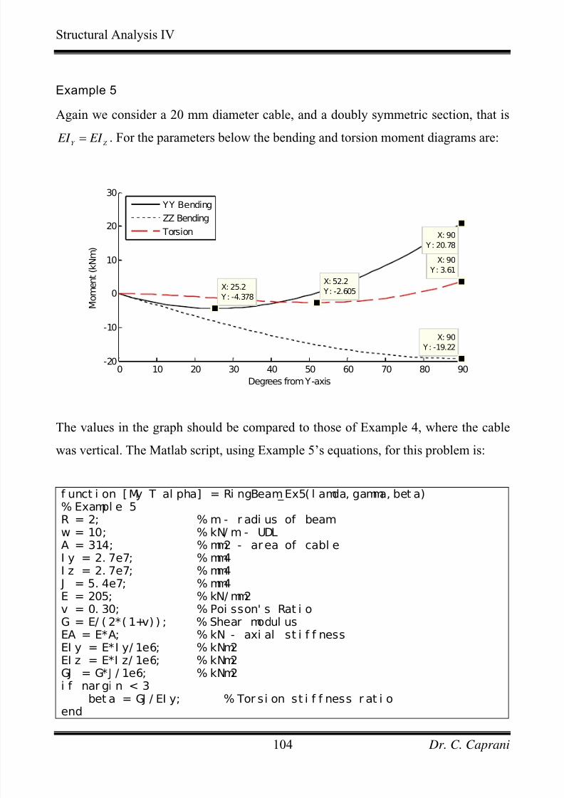
7/28/2019 Combined Structures 2009-10
http://slidepdf.com/reader/full/combined-structures-2009-10 104/106
Structural Analysis IV
Example 5
Again we consider a 20 mm diameter cable, and a doubly symmetric section, that is
Y Z EI EI = . For the parameters below the bending and torsion moment diagrams are:
0 10 20 30 40 50 60 70 80 90-20
-10
0
10
20
30
X: 90
Y: -19.22
X: 52.2 Y: -2.605
X: 90
Y: 3.61
X: 90
Y: 20.78
X: 25.2
Y: -4.378 M o m e n t ( k N m )
Degrees from Y-axis
YY Bending
ZZ Bending
Torsion
The values in the graph should be compared to those of Example 4, where the cable
was vertical. The Matlab script, using Example 5’s equations, for this problem is:
f unct i on [My T al pha] = Ri ngBeam_Ex5( l amda, gamma, bet a)% Exampl e 5R = 2; % m - r adi us of beamw = 10; % kN/ m - UDLA = 314; % mm2 - ar ea of cabl e
I y = 2. 7e7; % mm4I z = 2. 7e7; % mm4
J = 5. 4e7; % mm4E = 205; % kN/ mm2v = 0. 30; % Poi sson' s Rat i oG = E/ ( 2*( 1+v) ) ; % Shear modul usEA = E*A; % kN - axi al st i f f nessEI y = E*I y/ 1e6; % kNm2EI z = E*I z/ 1e6; % kNm2GJ = G*J / 1e6; % kNm2i f nar gi n < 3
bet a = GJ / EI y; % Tor si on st i f f ness r at i oend
Dr. C. Caprani104
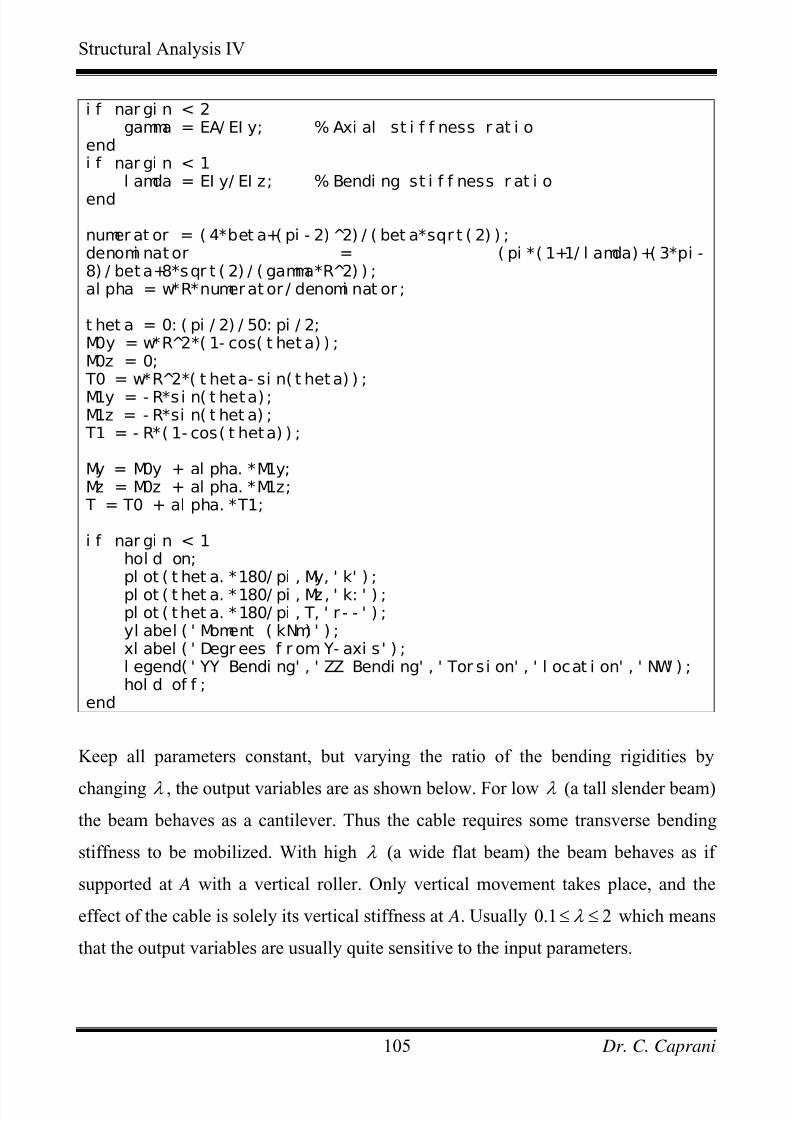
7/28/2019 Combined Structures 2009-10
http://slidepdf.com/reader/full/combined-structures-2009-10 105/106
Structural Analysis IV
i f nar gi n < 2gamma = EA/ EI y; % Axi al st i f f ness r at i o
endi f nar gi n < 1
l amda = EI y/ EI z; % Bendi ng st i f f ness r at i o
end
numer at or = ( 4*bet a+( pi - 2) 2̂) / ( bet a*sqr t ( 2) ) ;denomi nat or = ( pi *( 1+1/ l amda)+( 3*pi -8) / beta+8*sqr t ( 2) / ( gamma*R 2̂) ) ;al pha = w*R*numer at or / denomi nat or ;
t het a = 0: ( pi / 2) / 50: pi / 2;M0y = w*R 2̂*( 1- cos( t het a) ) ;M0z = 0;
T0 = w*R 2̂*( t heta- si n( t heta) ) ;
M1y = - R*s i n( t heta) ;M1z = - R*si n( t het a) ;
T1 = - R*( 1- cos( t heta) ) ;
My = M0y + al pha. *M1y;Mz = M0z + al pha. *M1z;
T = T0 + al pha. *T1;
i f nar gi n < 1hol d on;pl ot ( t het a. *180/ pi , My, ' k' ) ;pl ot ( t het a. *180/ pi , Mz, ' k: ' ) ;pl ot ( thet a. *180/ pi , T, ' r - - ' ) ;yl abel ( ' Moment ( kNm) ' ) ;xl abel ( ' Degr ees f r om Y- axi s ' ) ;l egend( ' YY Bendi ng' , ' ZZ Bendi ng' , ' Tor si on' , ' l ocat i on' , ' NW' ) ;hol d of f ;
end
Keep all parameters constant, but varying the ratio of the bending rigidities by
changing λ , the output variables are as shown below. For low λ (a tall slender beam)
the beam behaves as a cantilever. Thus the cable requires some transverse bending
stiffness to be mobilized. With high λ (a wide flat beam) the beam behaves as if
supported at A with a vertical roller. Only vertical movement takes place, and the
effect of the cable is solely its vertical stiffness at A. Usually 0.1 2λ ≤ ≤ which means
that the output variables are usually quite sensitive to the input parameters.
Dr. C. Caprani105
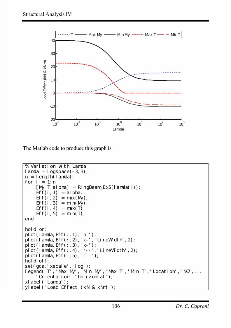
7/28/2019 Combined Structures 2009-10
http://slidepdf.com/reader/full/combined-structures-2009-10 106/106
Structural Analysis IV
10-3
10-2
10-1
100
101
102
103
-20
-10
0
10
20
30
40
Lamda
L o a d E f f e c t ( k N & k N m )
T Max My Min My Max T Min T
The Matlab code to produce this graph is:
% Var i at i on wi t h Lamda
l amda = l ogspace( - 3, 3) ;n = l ength( l amda) ;f or i = 1: n
[ My T al pha] = Ri ngBeam_Ex5( l amda( i ) ) ;Ef f ( i , 1) = al pha;Ef f ( i , 2) = max(My) ;Ef f ( i , 3) = mi n( My) ;Ef f ( i , 4) = max( T) ;Ef f ( i , 5) = mi n( T) ;
end


![Combined Capability List 23 October 2009[1]](https://img.pdfslide.net/doc/110x75/55cf947d550346f57ba260cf/combined-capability-list-23-october-20091.jpg)