_____________________________________________________________________________________

Christy L. Shostal. 2007. Combining GIS with a Hydraulic Flood Prediction Model: Developing a Custom GIS Tool for Near Real-Time Flood Inundation Mapping in the Fargo-Moorhead Portion of the Red River Basin. Volume 9, Papers in Resource Analysis. 17 pp. Saint Mary’s University of Minnesota University Central Services Press. Winona, MN. Retrieved (date) http://www.gis.smumn.edu

1

Combining GIS with a Hydraulic Flood Prediction Model: Developing a Custom GIS Tool for Near Real-Time Flood Inundation Mapping in the Fargo-Moorhead Portion of the Red River Basin Christy L. Shostal1, 2

1Department of Resource Analysis, Saint Mary’s University of Minnesota, Minneapolis, MN 55404;2Houston Engineering, Inc., Maple Grove, MN 55369 Keywords: Flood Forecast Display Tool, GIS, Red River of the North, Red River Basin, 1997, Flood Inundation Mapping, FLDWAV, DEM, LIDAR, Hydraulic Model, Unsteady Flow, ArcGIS, 3D Analyst, Spatial Analyst, Visual Basic, ArcObjects Abstract In preparation of another catastrophic flood, like the one experienced in 1997, Red River Basin stakeholders expressed the necessity for better methods for providing flood warnings. Traditional flood forecast hydrographs generated by the National Weather Service can be difficult for the general public to interpret and potential flood inundation extent can be very difficult to visualize. In 2005, the International Water Institute and the National Weather Institute retained Houston Engineering, Inc. to develop a custom flood forecasting display tool for near real-time flood inundation mapping for the Fargo, North Dakota-Moorhead, Minnesota Metropolitan Area. This tool was to consist of two major components: 1) a custom desktop GIS tool to be run by the NWS staff during flood evens to perform flood inundation mapping; and 2) an interactive Internet Map Server (IMS) application to display the map products to the public. This project focuses solely on the development of the custom desktop GIS tool for near real-time flood inundation mapping. The Flood Wave (FLDWAV) unsteady state hydraulic model, developed by the NWS, was used to provide water surface elevation forecasts. ArcObjects and Visual Basic for Applications (VBA), within ESRI’s ArcGIS, were the programming languages used to create the tool. The custom tool provides the public with an easy to understand spatial visualization of potential flood inundation. Introduction The Red River Basin (Basin) is prone to severe flooding approximately once every decade (Bourget, 2004). Flooding in the Basin in recent years has resulted in catastrophic economic damage, psychological damage, and loss of life. The flood of 1997 was particularly devastating. The city of Grand Forks, North Dakota suffered enormous

damage. The Fargo, North Dakota- Moorhead, Metropolitan Area (FMMA), also suffered severe damage during this flood event.

After the 1997 flood, Basin stakeholders expressed the need for better tools for forecasting and fighting floods. A number of stakeholders also stated that improved access to relevant GIS data for the area, such as Digital

Elevation Models (DEMs) and hydrologic features, would be imperative for creating such forecasting tools. In addition, it was noted that these data sets needed to be both of high quality and seamless across the basin to be of any value to flood forecasting (Deutschman, et al., 2006).

During flood events, the National Weather Service (NWS) issues water surface elevation forecasts for different gaging stations along the Red River of the North (Red River) and the Wild Rice River of North Dakota (Wild Rice River) as seen in Figure 1.

Figure 1. Example of NWS hydrograph.

These forecasts can be confusing to those without a background in water resources and the locations represented are hard to visualize. As a result, this data is commonly misinterpreted (Deutschman et al., 2006). The City of Fargo and the Province of Manitoba both have developed web applications that use pre-processed model results that show flood inundation at selected flood stages, such as the 100-year and 500-year floods.

In 2005, the International Water Institute (IWI) and the NWS retained Houston Engineering, Inc (HEI) to develop a custom desktop GIS tool, to be used by NWS staff, to perform near real-

time flood inundation mapping for the FFMA. The objective of this tool was to use an unsteady state hydraulic model to provide water surface elevation forecasts for the project area, to generate time series of near real-time depth grids and predicted flood inundation shapefiles. The FLDWAV model, developed by the NWS, was used to provide the forecast data. Deutschman et al. (2006) state “this model was chosen by the NWS for this project because of its demonstrated applicability to the Basin and ability to provide near real-time flood forecasts along the project extents of the Red River and Wild Rice River.” This model was also chosen because the NWS had 30 days of FLDWAV calibration files for the 1997 flood. These files were used for comparison of results and performing quality control.

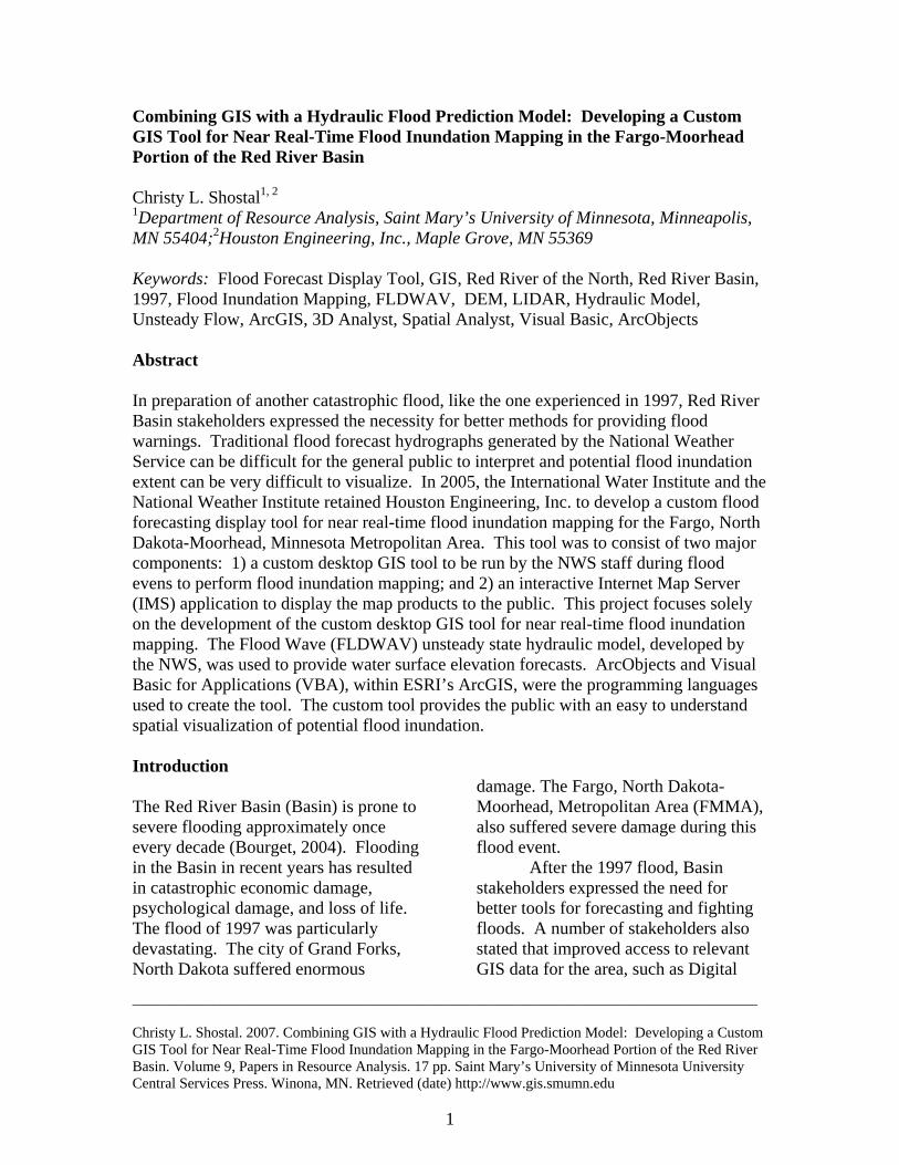
The tool would also analyze critical facilities in the FFMA, such as hospitals, police stations, and radio stations, to determine whether or not they were at risk of flooding. These products would provide an easy to understand visual representation of predicted flood inundation within the FFMA. The results would be uploaded to an interactive Internet Map Server (IMS) application, also to be developed by HEI. The inundation shapefiles and the depth grid for the peak flood would also be available to the public to download. This IMS application is hosted on the Red River Basin Decision Information Network (RRBDIN), an existing website that was developed by HEI (Figure 2). This project focuses solely on the development of the custom desktop GIS tool, hereby called the Flood Forecast Display Tool (FFDT).

A number of GIS tools already exist that are capable of mapping flood inundation, such as HEC-GeoRAS.

2

These programs all share one thing in common: only one water surface elevation file is mapped at a time. The challenge with this project is to develop a tool capable of looping through the time series of water elevation predictions generated by the FLDWAV model during flood events. In addition, the tool needs to run quickly enough that the results are still relevant by the time they are posted on the RRBDIN website.

Figure 2. Red River Basin Decision Information Network (RBDIN) website.

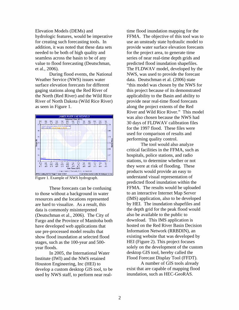
The geographic study area used

for this project covers the FFMA and extends just south of the confluence of the Wild Rice River with the Red River (Figure 3). The project area is approximately 140 square miles in size and consists of approximately 51 miles of the Red River and 20 miles of the Wild Rice River. The FFMA area was chosen for a number of important reasons: (1) high resolution topographic data is available, (2) stakeholder interest and cooperation is high, (3) the FFMA has the highest population density of any region within the U.S. portion of the Basin, and (4) moderate to severe flooding is a regular occurrence. Methods Planning

Figure 3. Project area located within the Fargo-Moorhead area of the Red River Basin.

Team Meetings The development of the FFDT began in April, 2006 and extended through December of the same year. The first step in the planning process was a series of team meetings which took place to brainstorm ideas for the overall project, to determine the requirements for the FFDT, and to prioritize the deliverables. These meetings determined that the FFDT had to meet the following key requirements:

1. Utilize Environmental Systems Research Institute’s (ESRI) ArcGIS ArcView software as the NWS does not have ArcEditor or ArcInfo;

2. Utilize ArcGIS Version 9.1, released at the time that this project was conducted;

3. Process within two hours or less such that the products could be posted prior to the next available forecast;

4. Operate such that a novice GIS user could run it;

3

5. Generate intuitive folders for ease of data transfer; and

6. Produce small enough data products such that they could be uploaded to the IMS application within the required time frame.

Development of Pseudo-Code Prior to writing any code, development of the FFDT tool began with the creation of a general flow path schematic of the conceptualized process. “Pseudo-code” was then developed to define the steps necessary to satisfy the project deliverables. Determining the desired deliverables provided clear starting and ending points and acted as a project outline. Re-examining the project deliverables at regular intervals ensured that the project was on track and that the objectives would be reached. A generalized flow chart of the required steps can be seen in Appendix A. Data A number of data sets were essential to the project to ensure that the most accurate inundation mapping would be conducted. These layers include the following:

1. Water surface elevation model; 2. High resolution topographic data; 3. Channel features;

a. Cross section locations; b. Areas protected by levees,

areas subject to ponding, areas subject to river flooding, and areas not mapped; and

c. Backwater areas. 4. Critical facilities locations.

To ensure that the most recent

and accurate versions of data sets were obtained, data was collected from the primary sources. For the spatial data sets NAD83, UTM, Zone 14 was the projection used. All of the data sets were examined and, if required, were reprojected. Water Surface Elevation Model The NWS uses the FLDWAV model to perform post flood analysis as well as real-time forecasting. FLDWAV is used for natural floods, as well as dam-break floods (Buan, 2003). The FLDWAV model takes into account current hydrologic conditions and is applied to an area for real-time forecasting. During periods of flooding in the project area, a water surface elevation time series is created by the NWS using FLDWAV.

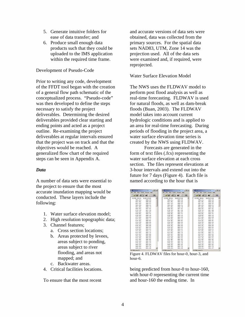
Forecasts are generated in the form of text files (.fcs) representing the water surface elevation at each cross section. The files represent elevations at 3-hour intervals and extend out into the future for 7 days (Figure 4). Each file is named according to the hour that is

Figure 4. FLDWAV files for hour-0, hour-3, and hour-6. being predicted from hour-0 to hour-160, with hour-0 representing the current time and hour-160 the ending time. In

4

addition to these files, a peak file (.fc1) is generated which shows the highest elevation reached at each cross section throughout the entire time series. Finally, a date file (.date) is generated which shows the start date and end date of the FLDWAV time series. For this project, the project team determined that mapping every FLDWAV file would be too time-consuming. In addition, at the scale being used, differences in water surface elevations would produce results that would not be visible to the human eye. Therefore, the decision was made that the FFDT would use the FLWAV files at 6-hour intervals. High Resolution Topographic Data High resolution topographic data was essential to represent a detailed ground elevation surface. A variety of Light Detection and Radar (LIDAR) collects have been completed in recent years within portions of the Basin. LIDAR data is capable of providing bare-earth vertical accuracies of less than six inches once post-processing has been performed to remove data points falling on objects that are impenetrable by the LIDAR (Bourget, 2004). The high accuracy of this data makes it very valuable for hydraulic modeling.

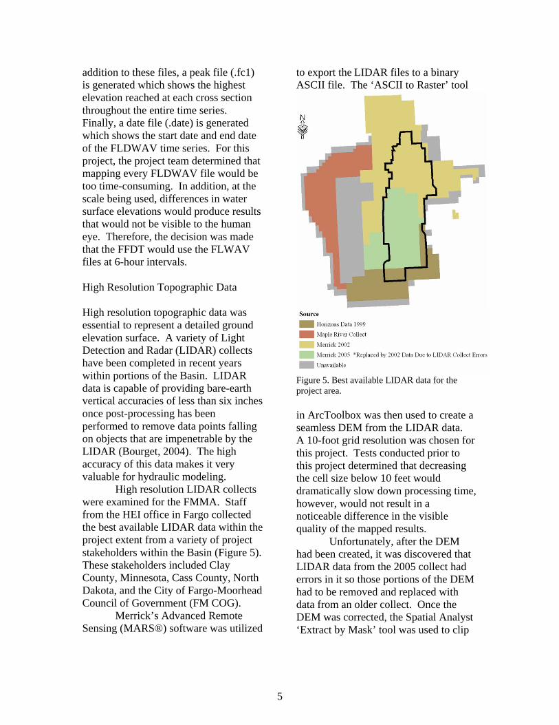
High resolution LIDAR collects were examined for the FMMA. Staff from the HEI office in Fargo collected the best available LIDAR data within the project extent from a variety of project stakeholders within the Basin (Figure 5). These stakeholders included Clay County, Minnesota, Cass County, North Dakota, and the City of Fargo-Moorhead Council of Government (FM COG).

Merrick’s Advanced Remote Sensing (MARS®) software was utilized

to export the LIDAR files to a binary ASCII file. The ‘ASCII to Raster’ tool

Figure 5. Best available LIDAR data for the project area.

in ArcToolbox was then used to create a seamless DEM from the LIDAR data. A 10-foot grid resolution was chosen for this project. Tests conducted prior to this project determined that decreasing the cell size below 10 feet would dramatically slow down processing time, however, would not result in a noticeable difference in the visible quality of the mapped results.

Unfortunately, after the DEM had been created, it was discovered that LIDAR data from the 2005 collect had errors in it so those portions of the DEM had to be removed and replaced with data from an older collect. Once the DEM was corrected, the Spatial Analyst ‘Extract by Mask’ tool was used to clip

5

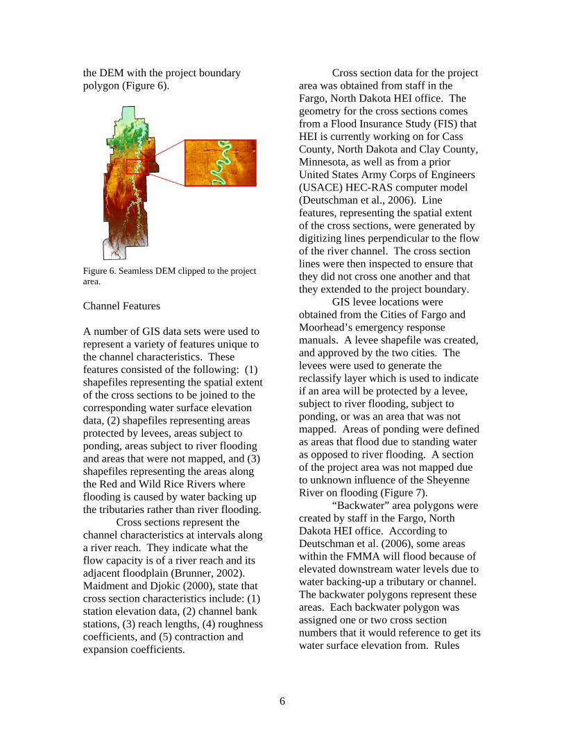
the DEM with the project boundary polygon (Figure 6).

Figure 6. Seamless DEM clipped to the project area. Channel Features A number of GIS data sets were used to represent a variety of features unique to the channel characteristics. These features consisted of the following: (1) shapefiles representing the spatial extent of the cross sections to be joined to the corresponding water surface elevation data, (2) shapefiles representing areas protected by levees, areas subject to ponding, areas subject to river flooding and areas that were not mapped, and (3) shapefiles representing the areas along the Red and Wild Rice Rivers where flooding is caused by water backing up the tributaries rather than river flooding.

Cross sections represent the channel characteristics at intervals along a river reach. They indicate what the flow capacity is of a river reach and its adjacent floodplain (Brunner, 2002). Maidment and Djokic (2000), state that cross section characteristics include: (1) station elevation data, (2) channel bank stations, (3) reach lengths, (4) roughness coefficients, and (5) contraction and expansion coefficients.

Cross section data for the project area was obtained from staff in the Fargo, North Dakota HEI office. The geometry for the cross sections comes from a Flood Insurance Study (FIS) that HEI is currently working on for Cass County, North Dakota and Clay County, Minnesota, as well as from a prior United States Army Corps of Engineers (USACE) HEC-RAS computer model (Deutschman et al., 2006). Line features, representing the spatial extent of the cross sections, were generated by digitizing lines perpendicular to the flow of the river channel. The cross section lines were then inspected to ensure that they did not cross one another and that they extended to the project boundary.

GIS levee locations were obtained from the Cities of Fargo and Moorhead’s emergency response manuals. A levee shapefile was created, and approved by the two cities. The levees were used to generate the reclassify layer which is used to indicate if an area will be protected by a levee, subject to river flooding, subject to ponding, or was an area that was not mapped. Areas of ponding were defined as areas that flood due to standing water as opposed to river flooding. A section of the project area was not mapped due to unknown influence of the Sheyenne River on flooding (Figure 7).

“Backwater” area polygons were created by staff in the Fargo, North Dakota HEI office. According to Deutschman et al. (2006), some areas within the FMMA will flood because of elevated downstream water levels due to water backing-up a tributary or channel. The backwater polygons represent these areas. Each backwater polygon was assigned one or two cross section numbers that it would reference to get its water surface elevation from. Rules

6

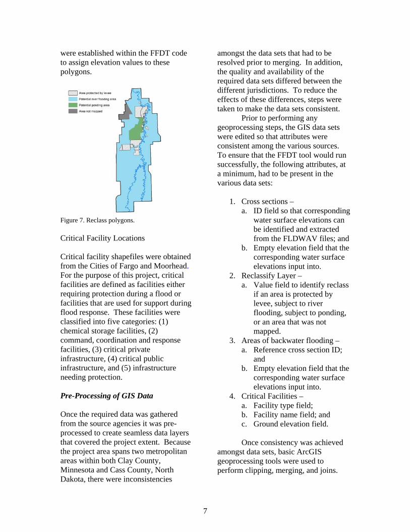
were established within the FFDT code to assign elevation values to these polygons.

Figure 7. Reclass polygons.

Critical Facility Locations Critical facility shapefiles were obtained from the Cities of Fargo and Moorhead. For the purpose of this project, critical facilities are defined as facilities either requiring protection during a flood or facilities that are used for support during flood response. These facilities were classified into five categories: (1) chemical storage facilities, (2) command, coordination and response facilities, (3) critical private infrastructure, (4) critical public infrastructure, and (5) infrastructure needing protection. Pre-Processing of GIS Data Once the required data was gathered from the source agencies it was pre-processed to create seamless data layers that covered the project extent. Because the project area spans two metropolitan areas within both Clay County, Minnesota and Cass County, North Dakota, there were inconsistencies

amongst the data sets that had to be resolved prior to merging. In addition, the quality and availability of the required data sets differed between the different jurisdictions. To reduce the effects of these differences, steps were taken to make the data sets consistent.

Prior to performing any geoprocessing steps, the GIS data sets were edited so that attributes were consistent among the various sources. To ensure that the FFDT tool would run successfully, the following attributes, at a minimum, had to be present in the various data sets:

1. Cross sections –

a. ID field so that corresponding water surface elevations can be identified and extracted from the FLDWAV files; and

b. Empty elevation field that the corresponding water surface elevations input into.

2. Reclassify Layer – a. Value field to identify reclass

if an area is protected by levee, subject to river flooding, subject to ponding, or an area that was not mapped.

3. Areas of backwater flooding – a. Reference cross section ID;

and b. Empty elevation field that the

corresponding water surface elevations input into.

4. Critical Facilities – a. Facility type field; b. Facility name field; and c. Ground elevation field.

Once consistency was achieved

amongst data sets, basic ArcGIS geoprocessing tools were used to perform clipping, merging, and joins.

7

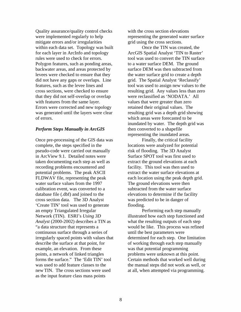
Quality assurance/quality control checks were implemented regularly to help mitigate errors and/or irregularities within each data set. Topology was built for each layer in ArcInfo and topology rules were used to check for errors. Polygon features, such as ponding areas, backwater areas, and areas protected by levees were checked to ensure that they did not have any gaps or overlaps. Line features, such as the levee lines and cross sections, were checked to ensure that they did not self-overlap or overlap with features from the same layer. Errors were corrected and new topology was generated until the layers were clear of errors. Perform Steps Manually in ArcGIS Once pre-processing of the GIS data was complete, the steps specified in the pseudo-code were carried out manually in ArcView 9.1. Detailed notes were taken documenting each step as well as recording problems encountered and potential problems. The peak ASCII FLDWAV file, representing the peak water surface values from the 1997 calibration event, was converted to a database file (.dbf) and joined to the cross section data. The 3D Analyst ‘Create TIN’ tool was used to generate an empty Triangulated Irregular Network (TIN). ESRI’s Using 3D Analyst (2000-2002) describes a TIN as “a data structure that represents a continuous surface through a series of irregularly spaced points with values that describe the surface at that point, for example, an elevation. From these points, a network of linked triangles forms the surface.” The ‘Edit TIN’ tool was used to add feature classes to the new TIN. The cross sections were used as the input feature class mass points

with the cross section elevations representing the generated water surface grid using the cross sections.

Once the TIN was created, the ArcGIS Spatial Analyst ‘TIN to Raster’ tool was used to convert the TIN surface to a water surface DEM. The ground surface DEM was then subtracted from the water surface grid to create a depth grid. The Spatial Analyst ‘Reclassify’ tool was used to assign new values to the resulting grid. Any values less than zero were reclassified as ‘NODATA.’ All values that were greater than zero retained their original values. The resulting grid was a depth grid showing which areas were forecasted to be inundated by water. The depth grid was then converted to a shapefile representing the inundated areas.

Finally, the critical facility locations were analyzed for potential risk of flooding. The 3D Analyst Surface SPOT tool was first used to extract the ground elevations at each facility. This tool was then used to extract the water surface elevations at each location using the peak depth grid. The ground elevations were then subtracted from the water surface elevations to determine if the facility was predicted to be in danger of flooding. Performing each step manually illustrated how each step functioned and what the resulting outputs of each step would be like. This process was refined until the best parameters were determined for each step. One limitation of working through each step manually was that potential programming problems were unknown at this point. Certain methods that worked well during the manual steps did not work as well, or at all, when attempted via programming.

8

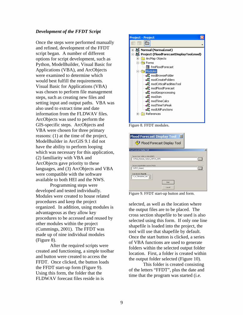
Development of the FFDT Script Once the steps were performed manually and refined, development of the FFDT script began. A number of different options for script development, such as Python, ModelBuilder, Visual Basic for Applications (VBA), and ArcObjects were examined to determine which would best fulfill the requirements. Visual Basic for Applications (VBA) was chosen to perform file management steps, such as creating new files and setting input and output paths. VBA was also used to extract time and date information from the FLDWAV files. ArcObjects was used to perform the GIS-specific steps. ArcObjects and VBA were chosen for three primary reasons: (1) at the time of the project, ModelBuilder in ArcGIS 9.1 did not have the ability to perform looping which was necessary for this application, (2) familiarity with VBA and ArcObjects gave priority to these languages, and (3) ArcObjects and VBA were compatible with the software available to both HEI and the NWS. Programming steps were developed and tested individually. Modules were created to house related procedures and keep the project organized. In addition, using modules is advantageous as they allow key procedures to be accessed and reused by other modules within the project (Cummings, 2001). The FFDT was made up of nine individual modules (Figure 8). After the required scripts were created and functioning, a simple toolbar and button were created to access the FFDT. Once clicked, the button loads the FFDT start-up form (Figure 9). Using this form, the folder that the FLDWAV forecast files reside in is

Figure 8. FFDT modules.

Figure 9. FFDT start-up button and form. selected, as well as the location where the output files are to be placed. The cross section shapefile to be used is also selected using this form. If only one line shapefile is loaded into the project, the tool will use that shapefile by default. Once the start button is clicked, a series of VBA functions are used to generate folders within the selected output folder location. First, a folder is created within the output folder selected (Figure 10).

This folder is created consisting of the letters “FFDT”, plus the date and time that the program was started (i.e.

9

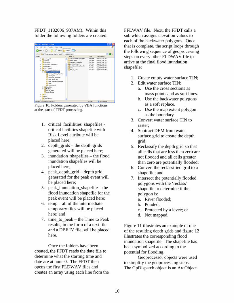
FFDT_1182006_937AM). Within this folder the following folders are created:

Figure 10. Folders generated by VBA functions at the start of FFDT processing.

1. critical_facililities_shapefiles - critical facilities shapefile with Risk Level attribute will be placed here;

2. depth_grids – the depth grids generated will be placed here;

3. inundation_shapefiles – the flood inundation shapefiles will be placed here;

4. peak_depth_grid – depth grid generated for the peak event will be placed here;

5. peak_inundation_shapefile – the flood inundation shapefile for the peak event will be placed here;

6. temp – all of the intermediate temporary files will be placed here; and

7. time_to_peak – the Time to Peak results, in the form of a text file and a DBF IV file, will be placed here.

Once the folders have been

created, the FFDT reads the date file to determine what the starting time and date are at hour-0. The FFDT then opens the first FLDWAV files and creates an array using each line from the

FFLWAV file. Next, the FFDT calls a sub which assigns elevation values to each of the backwater polygons. Once that is complete, the script loops through the following sequence of geoprocessing steps on every other FLDWAV file to arrive at the final flood inundation shapefile:

1. Create empty water surface TIN; 2. Edit water surface TIN;

a. Use the cross sections as mass points and as soft lines.

b. Use the backwater polygons as a soft replace.

c. Use the map extent polygon as the boundary.

3. Convert water surface TIN to raster;

4. Subtract DEM from water surface grid to create the depth grid;

5. Reclassify the depth grid so that all cells that are less than zero are not flooded and all cells greater than zero are potentially flooded;

6. Convert the reclassified grid to a shapefile; and

7. Intersect the potentially flooded polygons with the ‘reclass’ shapefile to determine if the polygon is: a. River flooded; b. Ponded; c. Protected by a levee; or d. Not mapped.

Figure 11 illustrates an example of one of the resulting depth grids and figure 12 illustrates the corresponding flood inundation shapefile. The shapefile has been symbolized according to the potential for flooding.

Geoprocessor objects were used to simplify the geoprocessing steps. The GpDispatch object is an ArcObject

10

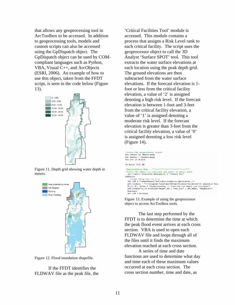
that allows any geoprocessing tool in ArcToolbox to be accessed. In addition to geoprocessing tools, models and custom scripts can also be accessed using the GpDispatch object. The GpDispatch object can be used by COM-compliant languages such as Python, VBA, Visual C++, and ArcObjects (ESRI, 2006). An example of how to use this object, taken from the FFDT script, is seen in the code below (Figure 13).

Figure 11. Depth grid showing water depth in meters.

Figure 12. Flood inundation shapefile.

If the FFDT identifies the FLDWAV file as the peak file, the

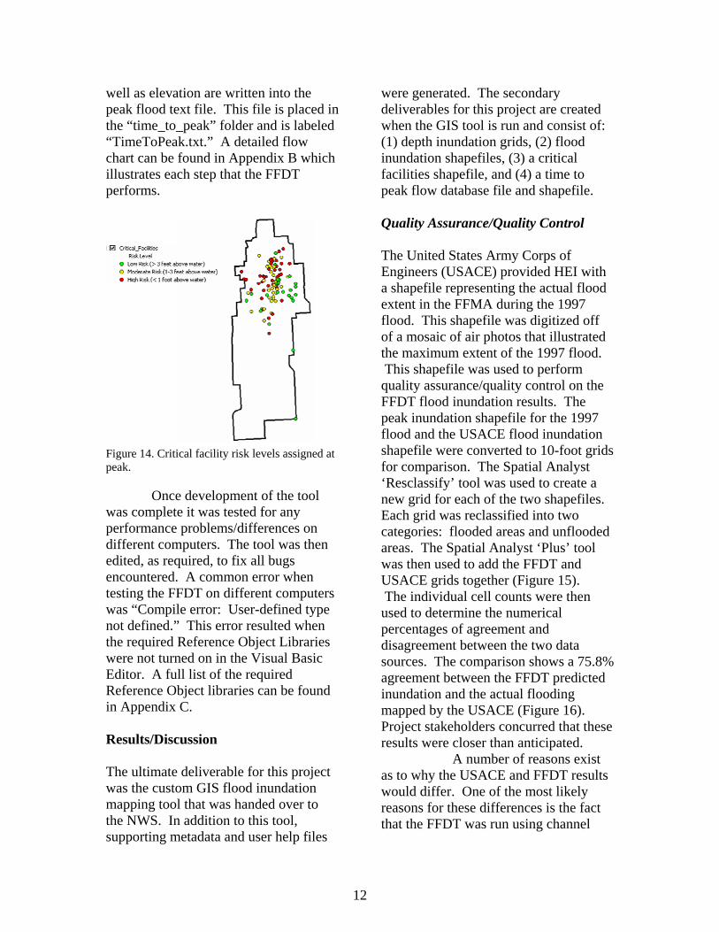
‘Critical Facilities Tool’ module is accessed. This module contains a process that assigns a Risk Level rank to each critical facility. The script uses the geoprocessor object to call the 3D Analyst ‘Surface SPOT’ tool. This tool extracts the water surface elevations at each location using the peak depth grid. The ground elevations are then subtracted from the water surface elevations. If the forecast elevation is 1-foot or less from the critical facility elevation, a value of ‘2’ is assigned denoting a high risk level. If the forecast elevation is between 1-foot and 3-feet from the critical facility elevation, a value of ‘1’ is assigned denoting a moderate risk level. If the forecast elevation is greater than 3-feet from the critical facility elevation, a value of ‘0’ is assigned denoting a low risk level (Figure 14).

Figure 13. Example of using the geoprocessor object to access ArcToolbox tools.

The last step performed by the

FFDT is to determine the time at which the peak flood event arrives at each cross section. VBA is used to open each FLDWAV file and loops through all of the files until it finds the maximum elevation reached at each cross section.

A series of time and date functions are used to determine what day and time each of these maximum values occurred at each cross section. The cross section number, time and date, as

11

well as elevation are written into the peak flood text file. This file is placed in the “time_to_peak” folder and is labeled “TimeToPeak.txt.” A detailed flow chart can be found in Appendix B which illustrates each step that the FFDT performs.

Figure 14. Critical facility risk levels assigned at peak.

Once development of the tool was complete it was tested for any performance problems/differences on different computers. The tool was then edited, as required, to fix all bugs encountered. A common error when testing the FFDT on different computers was “Compile error: User-defined type not defined.” This error resulted when the required Reference Object Libraries were not turned on in the Visual Basic Editor. A full list of the required Reference Object libraries can be found in Appendix C. Results/Discussion The ultimate deliverable for this project was the custom GIS flood inundation mapping tool that was handed over to the NWS. In addition to this tool, supporting metadata and user help files

were generated. The secondary deliverables for this project are created when the GIS tool is run and consist of: (1) depth inundation grids, (2) flood inundation shapefiles, (3) a critical facilities shapefile, and (4) a time to peak flow database file and shapefile. Quality Assurance/Quality Control The United States Army Corps of Engineers (USACE) provided HEI with a shapefile representing the actual flood extent in the FFMA during the 1997 flood. This shapefile was digitized off of a mosaic of air photos that illustrated the maximum extent of the 1997 flood. This shapefile was used to perform quality assurance/quality control on the FFDT flood inundation results. The peak inundation shapefile for the 1997 flood and the USACE flood inundation shapefile were converted to 10-foot grids for comparison. The Spatial Analyst ‘Resclassify’ tool was used to create a new grid for each of the two shapefiles. Each grid was reclassified into two categories: flooded areas and unflooded areas. The Spatial Analyst ‘Plus’ tool was then used to add the FFDT and USACE grids together (Figure 15). The individual cell counts were then used to determine the numerical percentages of agreement and disagreement between the two data sources. The comparison shows a 75.8% agreement between the FFDT predicted inundation and the actual flooding mapped by the USACE (Figure 16). Project stakeholders concurred that these results were closer than anticipated.

A number of reasons exist as to why the USACE and FFDT results would differ. One of the most likely reasons for these differences is the fact that the FFDT was run using channel

12

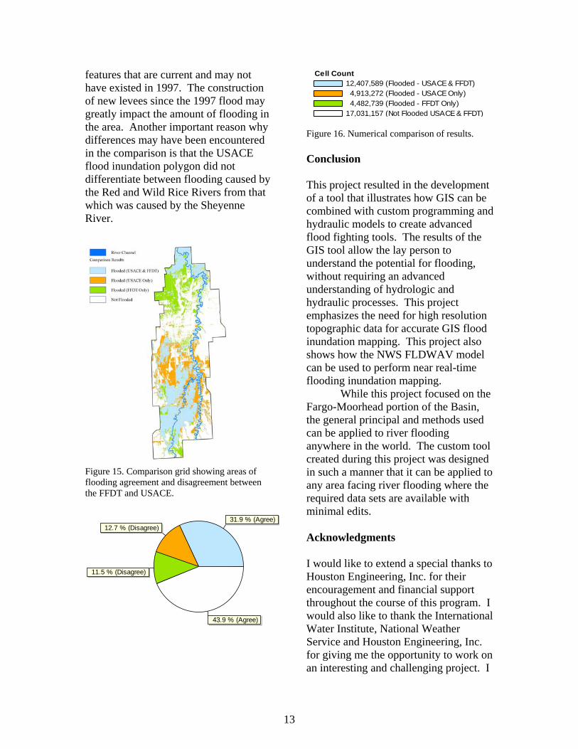
features that are current and may not have existed in 1997. The construction of new levees since the 1997 flood may greatly impact the amount of flooding in the area. Another important reason why differences may have been encountered in the comparison is that the USACE flood inundation polygon did not differentiate between flooding caused by the Red and Wild Rice Rivers from that which was caused by the Sheyenne River.

Figure 15. Comparison grid showing areas of flooding agreement and disagreement between the FFDT and USACE.

31.9 % (Agree)12.7 % (Disagree)

11.5 % (Disagree)

43.9 % (Agree)

Cell Count12,407,589 (Flooded - USACE & FFDT)4,913,272 (Flooded - USACE Only)4,482,739 (Flooded - FFDT Only)

17,031,157 (Not Flooded USACE & FFDT) Figure 16. Numerical comparison of results. Conclusion This project resulted in the development of a tool that illustrates how GIS can be combined with custom programming and hydraulic models to create advanced flood fighting tools. The results of the GIS tool allow the lay person to understand the potential for flooding, without requiring an advanced understanding of hydrologic and hydraulic processes. This project emphasizes the need for high resolution topographic data for accurate GIS flood inundation mapping. This project also shows how the NWS FLDWAV model can be used to perform near real-time flooding inundation mapping.

While this project focused on the Fargo-Moorhead portion of the Basin, the general principal and methods used can be applied to river flooding anywhere in the world. The custom tool created during this project was designed in such a manner that it can be applied to any area facing river flooding where the required data sets are available with minimal edits. Acknowledgments I would like to extend a special thanks to Houston Engineering, Inc. for their encouragement and financial support throughout the course of this program. I would also like to thank the International Water Institute, National Weather Service and Houston Engineering, Inc. for giving me the opportunity to work on an interesting and challenging project. I

13

would also like to thank the Department of Resource Analysis staff at Saint Mary’s University for their guidance. Special thanks also to Mike Juvrud for sharing some of his expansive programming knowledge with me. Finally, I would like to thank Troy Erickson for his continued patience, encouragement and guidance throughout the course of this program. References Bourget, P. 2004. Basin-level digital

elevation models: Availability and Applications, the Red River of the North basin case study. IWR Report 04-R-1. US Army Corps of Engi- neers Civil Works Research and Development Program.

Brunner, G. W. 2002. HEC-RAS: River Analysis System Hydraulic Reference Manual. Davis, CA. US Army Corps of Engineers.

Buan, Steven D. April, 2003. FLDWAV Model: A One-Dimensional Unsteady Flow Model for the Red River of the North. Paper presented at the 2003 Red River Basin Institute 1st International Water Conference, Moorhead, Minnesota.

Cummings, S. 2001. VBA for Dummies. New York: Hungry Minds, Inc.

Deutschman, M., Fischer, B. and Shostal, C. 2006. Project Documentation: Red River Basin Flood Forecast Display Tool. Available from Houston Engineering, Inc. Maple Grove, MN.

Environmental Systems Research Institute. 2006. How To: Execute geoprocessing tools from within VBA. Retrieved July 31, 2007 from http://support.esri.com/index.cfm?fa=knowledgebase.techarticles.articleShow&d=31110.

Environmental Systems Research Institute. 2000-2002. Using ArcGIS 3D Analyst: GIS by ESRI. Redlands: ESRI Press.

Maidment, D. & Djokic, D. 2000. Hydrologic and hydraulic modeling support with Geographic Information Systems. Redlands: ESRI Press.

14

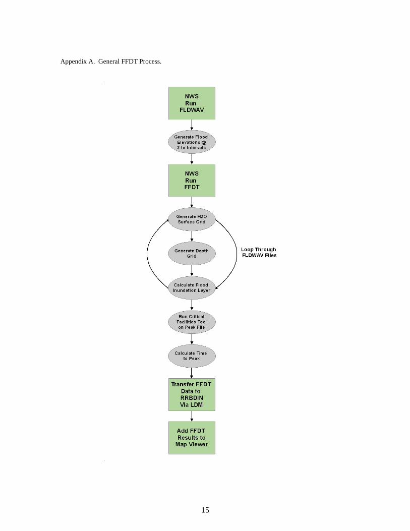
Appendix A. General FFDT Process.

15

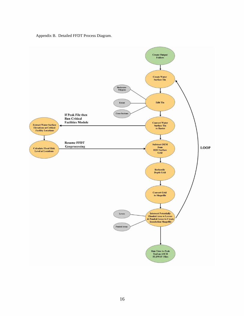
Appendix B. Detailed FFDT Process Diagram.

16

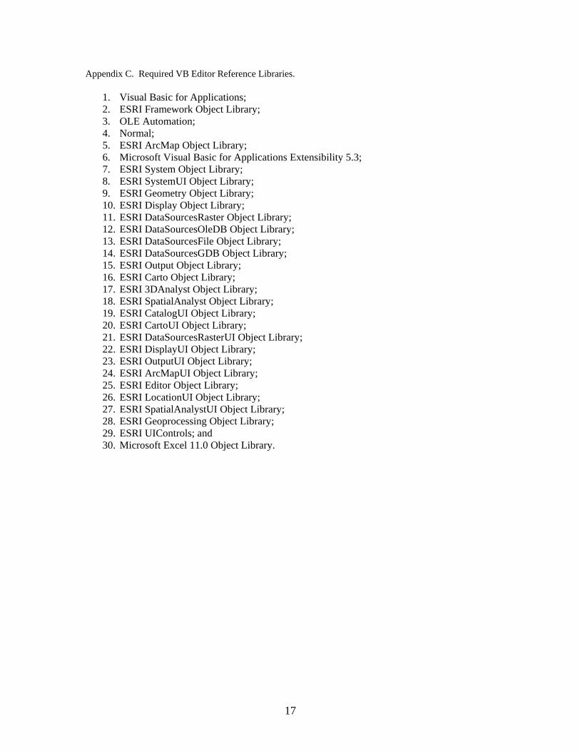
Appendix C. Required VB Editor Reference Libraries.

1. Visual Basic for Applications; 2. ESRI Framework Object Library; 3. OLE Automation; 4. Normal; 5. ESRI ArcMap Object Library; 6. Microsoft Visual Basic for Applications Extensibility 5.3; 7. ESRI System Object Library; 8. ESRI SystemUI Object Library; 9. ESRI Geometry Object Library; 10. ESRI Display Object Library; 11. ESRI DataSourcesRaster Object Library; 12. ESRI DataSourcesOleDB Object Library; 13. ESRI DataSourcesFile Object Library; 14. ESRI DataSourcesGDB Object Library; 15. ESRI Output Object Library; 16. ESRI Carto Object Library; 17. ESRI 3DAnalyst Object Library; 18. ESRI SpatialAnalyst Object Library; 19. ESRI CatalogUI Object Library; 20. ESRI CartoUI Object Library; 21. ESRI DataSourcesRasterUI Object Library; 22. ESRI DisplayUI Object Library; 23. ESRI OutputUI Object Library; 24. ESRI ArcMapUI Object Library; 25. ESRI Editor Object Library; 26. ESRI LocationUI Object Library; 27. ESRI SpatialAnalystUI Object Library; 28. ESRI Geoprocessing Object Library; 29. ESRI UIControls; and 30. Microsoft Excel 11.0 Object Library.

17