Combining Multiple Hypothesis Testing with …1fd18a91-bc61-4bf3-b798-cd38a91c5399/Mi… · Combining Multiple Hypothesis Testing with Machine Learning Increases the Statistical Power

1Scientific RepoRts | 6:36671 | DOI: 10.1038/srep36671

www.nature.com/scientificreports

Combining Multiple Hypothesis Testing with Machine Learning Increases the Statistical Power of Genome-wide Association StudiesBettina Mieth1,*, Marius Kloft2,*, Juan Antonio Rodríguez3,*, Sören Sonnenburg4, Robin Vobruba1, Carlos Morcillo-Suárez3, Xavier Farré3, Urko M. Marigorta5, Ernst Fehr6,†, Thorsten Dickhaus7,†, Gilles Blanchard8,†, Daniel Schunk9,†, Arcadi Navarro3,10,11,† & Klaus-Robert Müller1,12,†

The standard approach to the analysis of genome-wide association studies (GWAS) is based on testing each position in the genome individually for statistical significance of its association with the phenotype under investigation. To improve the analysis of GWAS, we propose a combination of machine learning and statistical testing that takes correlation structures within the set of SNPs under investigation in a mathematically well-controlled manner into account. The novel two-step algorithm, COMBI, first trains a support vector machine to determine a subset of candidate SNPs and then performs hypothesis tests for these SNPs together with an adequate threshold correction. Applying COMBI to data from a WTCCC study (2007) and measuring performance as replication by independent GWAS published within the 2008–2015 period, we show that our method outperforms ordinary raw p-value thresholding as well as other state-of-the-art methods. COMBI presents higher power and precision than the examined alternatives while yielding fewer false (i.e. non-replicated) and more true (i.e. replicated) discoveries when its results are validated on later GWAS studies. More than 80% of the discoveries made by COMBI upon WTCCC data have been validated by independent studies. Implementations of the COMBI method are available as a part of the GWASpi toolbox 2.0.

The goal of genome-wide association studies (GWAS) (e.g. the WTCCC study1) is to examine the relationship between genetic markers such as single-nucleotide polymorphisms (SNPs) and individual traits, which are usu-ally complex diseases or behavioral characteristics. Generally, a large number of statistical tests are performed in parallel, each SNP being individually tested for association2–4. The standard approach consists of computing individual, SNP-specific p-values corresponding to a statistical association test and comparing these p-values against some given significance threshold (say t*), meaning that precisely those SNPs with p-values smaller than t*are declared to be associated with the trait4–6. We refer to this approach as raw p-value thresholding (RPVT) and review some standard methods for choosing t* for the purpose of controlling multiple type I error rates

1Machine Learning Group, Technische Universität Berlin, Berlin, 10587, Germany. 2Department of Computer Science, Humboldt University of Berlin, Berlin, 10099, Germany. 3Institut de Biología Evolutiva (CSIC-UPF). Departament de Ciències Experimentals i de la Salut. Universitat Pompeu Fabra, Barcelona, 08003, Spain. 4TomTom Research, Berlin, 12555, Germany. 5School of Biology, Georgia Institute of Technology, Atlanta, 30332, GA, USA. 6Department of Economics, Laboratory for Social and Neural Systems Research, University of Zurich, Zurich, 8006, Switzerland. 7Institute for Statistics (FB 3), University of Bremen, Bremen, 28359, Germany. 8Department of Mathematics, University of Potsdam, Potsdam, 14476, Germany. 9Department of Economics, University of Mainz, Mainz, 55099, Germany. 10Institució Catalana de Recerca i Estudis Avançats (ICREA), Barcelona, 08010, Spain. 11Center for Genomic Regulation (CRG), Barcelona Institute of Science and Technology (BIST), Barcelona, 08003, Spain. 12Department of Brain and Cognitive Engineering, Korea University, Seoul, Republic of Korea. *These authors contributed equally to this work. †These authors jointly directed this work. Correspondence and requests for materials should be addressed to E.F. (email: [email protected]) or D.S. (email: [email protected]) or A.N. (email: [email protected])

received: 31 May 2016

Accepted: 06 October 2016

Published: 28 November 2016

OPEN

mailto:[email protected]



www.nature.com/scientificreports/


(in particular, the family-wise error rate (FWER) and the expected number of false rejections (ENFR)) in the Methods Section.

According to the GWAS catalog7,8 (last accessed 03-07-2015), the more than 1,400 GWAS published so far have led to the identification of more than 11,000 SNPs associated with about 800 human diseases and anthropo-metric traits with p-values using t* = 1 × 10−5.

However, variants reported by GWAS tend to explain only small fractions of individual traits, and most of the heritability accounting for many complex diseases remains unexplained — a phenomenon usually referred to as the “mystery of missing heritability”4,9. There are several possible (not mutually exclusive) explanations for that phenomenon10–13. One frequently discussed possibility is that epistatic interactions between loci are ignored both in current heritability estimates and in usual testing procedures12,14. In addition to this issue, another shortcoming of current approaches based on testing each SNP independently is that they disregard any correlation structures among the set of SNPs under investigation that are introduced by both population genetics (linkage disequilib-rium, LD) and biological relations (e.g. functional relationships between genes). The latter issue by itself is likely to introduce confounding factors and artifacts, implying a loss in statistical power15 and a lack of reliable insights about genotype-phenotype associations.

In this work, we propose a novel methodology — COMBI — that is a principled, reliable, and replicable method for identifying significant SNP-phenotype associations. The core idea is a two-step algorithm consisting of

1. a machine learning and SNP selection step that drastically reduces the number of candidate SNPs by select-ing only a small subset of the most predictive SNPs; and

2. a statistical testing step where only the SNPs selected in step 1 are tested for association.

The main idea underlying COMBI is the use of the state-of-the-art machine learning technique support vector machine (SVM)16–18 in the first step. Crucially, this method is tailored to predict the target output (here, the phe-notype) from high-dimensional data with a possibly complex, unknown correlation structure. In our application, the SVM is trained using the complete SNP data of one chromosome. Thus, the first step acts as a filter, indicating SNPs that are relevant for phenotype classification with either high individual effects or effects in combination with the rest of SNPs, while discarding artifacts due to the correlation structure. The second step uses multiple statistical hypotheses testing for a quantitative assessment of individual relevance of the filtered SNPs. All in all, the two steps extract complementary types of information, which are combined in the final output. Importantly, the calibration of the method is such that a global statistical error criterion is controlled for the entire procedure consisting of steps 1 and 2.

The following section first introduces the methodology in a summary paragraph and in Fig. 1; then, the Methods Section continues to explain the method in more detail with some references to Supplementary Section 1. An overview of related machine learning work is given in the Discussion Section. The performance of the COMBI method is reported in the Results Section, Supplementary Sections 2 and 3; where we also include and discuss the highly favorable comparisons with the algorithms that could potentially compete with the COMBI method. Note that COMBI yields better prediction with fewer false (i.e. non-replicated) and more true (i.e. replicated) discover-ies when its results are validated on later, larger GWAS studies.

Implementations of the COMBI method are available in R, MATLAB, and JAVA, as a part of the GWASpi toolbox 2.0 (https://bitbucket.org/gwas_combi/gwaspi/).

MethodsSummary of The COMBI Method. Figure 1 shows a graphical representation of the COMBI method.

Input: a sample of observed genotypes {xi*} and corresponding phenotypes {yi}. We represent the j-th SNP of the i-th subject with a binary genotypic encoding, where xij = (1, 0, 0), xij = (0, 1, 0), or xij = (0, 0, 1), depending on the number of minor alleles. We assume a binary phenotype, i.e., yi ∈ {+ 1, − 1}.

(I) Machine learning and SNP-selection step (colored in red).Based on the sample, an SVM is trained. The SVM returns a linear function f(x) = wTx, the sign of f(x) is a predic-tion of the unknown phenotype of a previously unseen genotype x. The absolute value |wj| of the corresponding component of the parameter vector w is interpreted for each SNP j as a measure of importance for the prediction function.The parameter vector w is then post-processed through a p-th-order moving average filter with window size l, that is, | | = ∑ = − −

+ −w w:jnew

h j ld j l

hp

max(1, ( 1)/2)min( , ( 1)/2)p . Finally, the SNPs corresponding to the k largest values of the

scores are selected; all other SNPs are discarded.

(II) Statistical testing step (colored in blue).A hypothesis test (carried out as a χ2 test) is performed for each of the selected SNPs. Those SNPs with p-value less than a significance threshold t* are returned. The threshold t* is calibrated using a permutation-based method over the whole procedure consisting of the machine learning selection and statistical testing steps. See Algorithm 2 for details.

Problem Setting and Methodology. In this section, we formally describe the statistical problem under investigation and propose a novel methodology for tackling it — based on a combination of machine learning and statistical testing techniques.

Problem Setting and Notation. Let n denote the number of subjects in the study and d the number of SNPs under investigation. Given a sample of observed genotypes = ∈

≤ ≤ ≤ ≤×x x( )ij i n j d

n d1 ,1

3 and corresponding

https://bitbucket.org/gwas_combi/gwaspi/



phenotypes = … ∈y y y( , , )nn

1 , each xi* and each x*j corresponds to a subject and a SNP, respectively. A binary feature encoding is employed, where xij = (1, 0, 0), xij = (0, 1, 0), or xij = (0, 0, 1) depending on the number of minor alleles in SNP j of subject i. This paper focuses on binary phenotypes, i.e., yi ∈ {+ 1, − 1} for all i = l, … , n. The data for one particular SNP can be summarized in a contingency table (See Table 1).

The numbers nik denote the number of cases (i = 1) and controls (i = 2), respectively, which exhibit the geno-type corresponding to column k. Notice that the row sums n1. and n2. are fixed and non-random by the experi-mental design (case-control study). Hence, the random vectors (n11, n12, n13)T and (n21, n22, n23)T follow a multinomial distribution with three categories, sample sizes n1. and n2., respectively; and unknown vectors of probabilities p1 = (p11, p12, p13)T and p2 = (p21, p22, p23)T, respectively. The parameter ϑ = ϑ

= …( )j j d1, ,

of the statis-

tical model for the whole study thus consists of all such pairs ϑ = p p( , )jj j

1( )

2( ) of multinomial probability vectors,

one for each of the d SNPs under investigation. For every SNP j, we are interested in testing the null hypothesis =p pH :j

j j1( )

2( ), where we introduced the superscript j to indicate the SNP. This hypothesis is equivalent to the null

hypothesis that the genotype at locus j is independent of the binary trait of interest. Two standard asymptotic tests for Hj versus its two-sided alternative Kj (genotype j is associated with the trait) are: the chi-square test for associ-ation and the Cochran-Armitage trend test (see, e.g., Sections 3.2.1 and 5.3.5 of the monograph by Agresti19). Both tests employ test statistics which are asymptotically (as min(n1., n2.) tends to infinity) chi-square distributed under Hj; the number of degrees of freedom equals 2 for the chi-square test for association, and 1 for the Cochran-Armitage trend test. Thus, p-values (pj: 1 ≤ j ≤ d) corresponding to these tests can be calculated by applying the upper-tail distribution function of the chi-square distribution with the corresponding degrees of freedom to the observed values of these statistics, and this for every SNP. Observe that the test statistics obtained for different SNPs will be highly correlated if these SNPs are in strong LD to each other; consequently, the corre-sponding p-values will also exhibit strong dependencies20,21.

Figure 1. The COMBI method - Summary and illustration of the methodology. Receiving genotypes and corresponding phenotypes of a GWAS as input, the COMBI method first applies a machine learning step to select a set of candidate SNPs and then calculates p-values and corresponding significance thresholds in a statistical testing step.

A1A1 A1A2 A2A2 ∑

Y = + 1 n11 n12 n13 n1.

Y = − 1 n21 n22 n23 n2.

∑ n0.1 n0.2 n0.3 n

Table 1. Tabular representation of single SNP data. Single SNP data are summarized in categories according to phenotypes (cases, Y = + 1, and controls, Y = − 1) and genotypes (A1A1, A1A2 and A2A2). The numbers nik denote the numbers of individuals within the corresponding groups. n is the total number of subjects in the study.



RPVT declares a SNP j significantly associated with the trait if pj ≤ t*. If there was a single test to perform (i.e., d = 1), then t* would be taken as a pre-defined significance level α , as in the classical approach to statistical hypothesis testing. In multiple testing, however, the threshold t* is modified to take the multiplicity of the problem (the fact that d > 1) into account. The simplest method is the so-called Bonferroni correction, = α⁎t

d. This choice guaran-

tees that the FWER (that is, the probability of one or more erroneously reported associations) of the multiple test is bounded by α . A variety of other RPVT methods are explained, for instance, in the monograph by Dickhaus22.

Proposed workflow. The Bonferroni correction can only attain the prescribed FWER upper bound, and there-fore have maximal power, if the p-values (pj:1 ≤ j ≤ d) do not exhibit strong (positive) dependencies, an assumption which is violated in GWAS due to strong LD in blocks of SNPs. An alternative way to calibrate the threshold t* for FWER control, taking the dependencies into account, is the Westfall-Young permutation procedure23, which con-trols the FWER under an assumption termed subset pivotality (see Westfall and Young23 as well as Dickhaus and Stange21). Furthermore, Meinshausen et al.24 proved that this permutation procedure is asymptotically optimal in the class of RPVT procedures, provided that the subset pivotality condition is fulfilled. However, for RPVT the indi-vidual p-value for association of the j-th SNP only depends on x*j and thus ignores the possible correlations with the rest of the genotype – which could yield additional information. By contrast, machine learning approaches aimed at prediction try to take the information of the whole genotype into account at once, and thus implicitly consider all possible correlations, to strive for an optimal prediction of the phenotype. Based on this observation, we propose Algorithm 1 combining the advantages of the two techniques, consisting of the following two steps:

• the machine learning step, where an appropriate subset of candidate SNPs is selected, based on their relevance for prediction of the phenotype;

• the statistical testing step, where a hypothesis test is performed together with a Westfall-Young type threshold calibration for each SNP.

Additionally, a filter first processes the weight vector w output in the machine learning step before using it for the selection of candidate SNPs. The above steps are discussed in more detail in the following sections.

The machine learning and SNP selection step. The goal in machine learning is to determine, based on the sample, a function f(x) that predicts the unknown phenotype y based on the observation of genotype x. It is crucial to require such a function to not only capture the sample at hand, but to also generalize, as well as possible, to new and unseen measurements, i.e., the sign of f(x) is a good predictor for y for previously unseen patterns x and labels y. We consider linear models of the form fw,b(xi*) = wTxi* + b in this paper. A popular approach to learn-ing such a model is given by the SVM16–18, which determines the parameter w of the model by solving, for C > 0, the following optimization problem:

∑∈ + − .=

⁎w w C y w xargmin max(0, 1 )(1)w

i

n

i i22

1

T

The problem above is similar to regression problems and can be interpreted as follows: we aim to minimize the trade-off (controlled by C) between a vector w with small norm (the term on the left-hand side) and small errors on the data (the term on the right-hand side). Once a classification function f has been determined by solving the above optimization problem, it can be used to predict the phenotype of any genotype by putting

= = .y f x w xsign( ( )) sign( ) (2)new new newT

The above equation shows that the largest components (in absolute value) of the vector w (called SVM param-eter or weight vector) also have the most influence on the predicted phenotype. Note that the weights vector contains three values for each position due to the feature embedding, which encodes each SNP with three binary variables. To convert the vector back to the original length, we simply take the average over the three weights. We also include an offset by including a constant feature that is all one.

Considering that the use of SVM weights as importance measures is a standard approach25, for each j the score abs(wj) can be interpreted as a measure for the importance of the j-th SNP for the phenotype prediction task. The main idea is to select only a small number k of candidate SNPs before statistical testing, namely those SNPs having the largest scores. Based on preliminary experiments, we noticed that the introduction of the following additional post-processing of the SVM parameter vector was beneficial before SNP selection: a pth-order moving average filter is applied as follows:

∑== − −

+ −

w w:(3)

jnew

k j l

d j l

kp

max(1, ( 1)/2)

min( , ( 1)/2)p

where l ∈ 1, … , d denotes a fixed filter length (required to be an odd number). The value p ∈ ]0, ∞ [ is a free parameter; in the case p = 1, a standard moving average filter is obtained.

The statistical testing step. In the statistical testing step (see Summary of the COMBI method and Fig. 1), we apply p-value thresholding only to the k p-values which correspond to the SNPs with largest filtered SVM weights. Calculation of these p-values is performed exactly as described above for RPVT, with the only modifica-tion that p-values for SNPs not ranked among the top k in terms of their filtered SVM weights are set to 1, without calculating a test statistic.



The methodological challenge now consists of finding a threshold t* for the remaining k p-values such that the FWER is controlled for the multiple test which the entire workflow defines (SVM training, filtering of weights, p-value calculation, p-value thresholding). To this end, we investigated prior approaches26,27 based on sample splitting meaning that the selection of k SNPs is done on one (randomly chosen) sub-sample of individuals, while the p-value calculation and thresholding for the selected SNPs is performed on another. In this scheme, and regardless of which SNP selection method used on the first sub-sample, a Bonferroni-type threshold = α⁎t

k guar-

antees FWER control at level α for the p-values computed on the second sub-sample. Since k ≪ d, this correction is much less conservative than the original Bonferroni correction using all SNPs. However, this is severely miti-gated by the loss of power in the p-values due to the sample splitting. In fact, computer simulations (See Supplementary Section 2.2.4.) indicated very low power for detecting true associations with such a method because of the reduced sample size for calculation of test statistics and p-values.

Our suggestion is to re-sample the entire workflow of Fig. 1, thus following a Westfall and Young23 type proce-dure, and to choose t* based on the permutation distribution of the re-sampled p-values.

In summary, the proposed methodology is formally stated as Algorithm 1.

Algorithm 1The Combi Method.Require: genotypes x = (xij) and phenotypes y = (yi), a reasonable upper bound k ∈ {1, … , d} for the number of informative SNPs, and an FWER level α 1: train an SVM using genotypes x and phenotypes y, resulting in scores w1, … , wd

2: filter the weights w1, … , wd according to (3)3: let w*(k) denote the k-th largest of the wj’s in absolute value and re-number the

corresponding positions from 1, … , k4: for all j = 1,… ,k do5: compute the p-value of the j-th SNP pj(x*j, y)6: end for7: decide that SNP j is associated with the trait if wj ≥ w*(k) and pj < t*, where

t* ≡ t*(k, a) is chosen as the α -quantile of the permutation distribution of the smallest of the k p-values (see Algorithm 2 for details)

Return predicted set of informative SNPs.

FWER control at level α of the multiple test defined by Algorithm 1 can be proven under a relaxed form of the subset pivotality condition, the validity of which is checked empirically in Supplementary Sections 2.2.1 and 2.2.2. To describe this condition formally, let 0 denote any probability measure under the global null hypothesis of no informative SNPs in {1, … , d} at all. We assume that the following condition holds true: Let p* denote the smallest of the k p-values corresponding to the positions picked by the SVM method for which the null hypothesis of no association between SNP and trait is true. Regarding p* as a random variable, assume that its distribution under the true data-generating distribution ϑ (which is unknown) is stochastically not smaller than under 0.

The distribution under 0 of the k p-values corresponding to positions chosen by applying the SVM method is now estimated by the resampling procedure given below as Algorithm 2. The algorithm repeatedly assigns a random permutation of the phenotypes yπ(1), … , yπ(n) to the observed genotypes x1*, … , xn*. The empirical lower α-quantile of the smallest of these k p-values is then a valid choice for t* in the sense that the FWER for the entire procedure defined by Algorithm 1 is bounded by α.

Algorithm 2Resampling-based threshold determination for Combi method.Require: genotypes x = (xij) and phenotypes y = (yi), the number k ∈ {1, … , d} as in Algorithm 1, an FWER level α , and a number B of Monte Carlo repetitions1: for b = 1, … , B do2: pick a random permutation π and set y(b) = (yπ(1), … , yπ(n))3: carry out steps 1–6 in Algorithm 1 with taking y(b) as phenotypes, resulting in

corresponding p-values pj(x*j, y(b))4: store the smallest of the k computed p-values as pmin

(b). 5: end for6: Order the ≤ ≤p b B: 1b

min( ) increasingly as ≤ ≤p b B( : 1 )b

ordered( ) .

Return the value α∗p Bordered( )



Note that the choice k = d leads to skipping the SVM step and arriving at the popular MinP procedure, origi-nally proposed in Westfall and Young23. Following the argumentation in Dudoit and van der Laan28, it is also possible to control the generalized FWER (gFWER) with parameter l ≥ 1with the aforementioned resampling scheme as well as the ENFR. For gFWER control with parameter l, one has to consider the (l + 1)th-smallest of the re-sampled p-values, instead of p b

min( ) in Algorithm 2. For ENFR control, one has to store all B * k computed

p-values and determine the p-value threshold that leads to an average number of rejections (over the B Monte Carlo repetitions) which matches the desired ENFR level. Moreover, so-called augmentation techniques28 can be utilized to control the false discovery rate (FDR) instead of the FWER.

ResultsValidation. Validation using simulated phenotypes. To assess the performance of the proposed COMBI method in comparison to other methods in a controlled environment, we conducted a number of simulation experiments with semi-real data. A block of 10,000 genotypes were taken from real WTCCC data1 without break-ing linkage, but the phenotypes were synthetically generated according to a known model. This ensures that the “basic truth” is known (allowing us to compute the number of true and false positives for each method in the comparison). We show that COMBI outperforms the most commonly used methods for GWAS on these data sets. For instance, it achieves higher true positive rates for all family-wise error levels than any other method that we have investigated26,29,30, including RPVT. In comparison to RPVT, the gain in true positive rate is up to 80%. For a detailed description and analysis of the semi-real data simulations, see Supplementary Section 2.

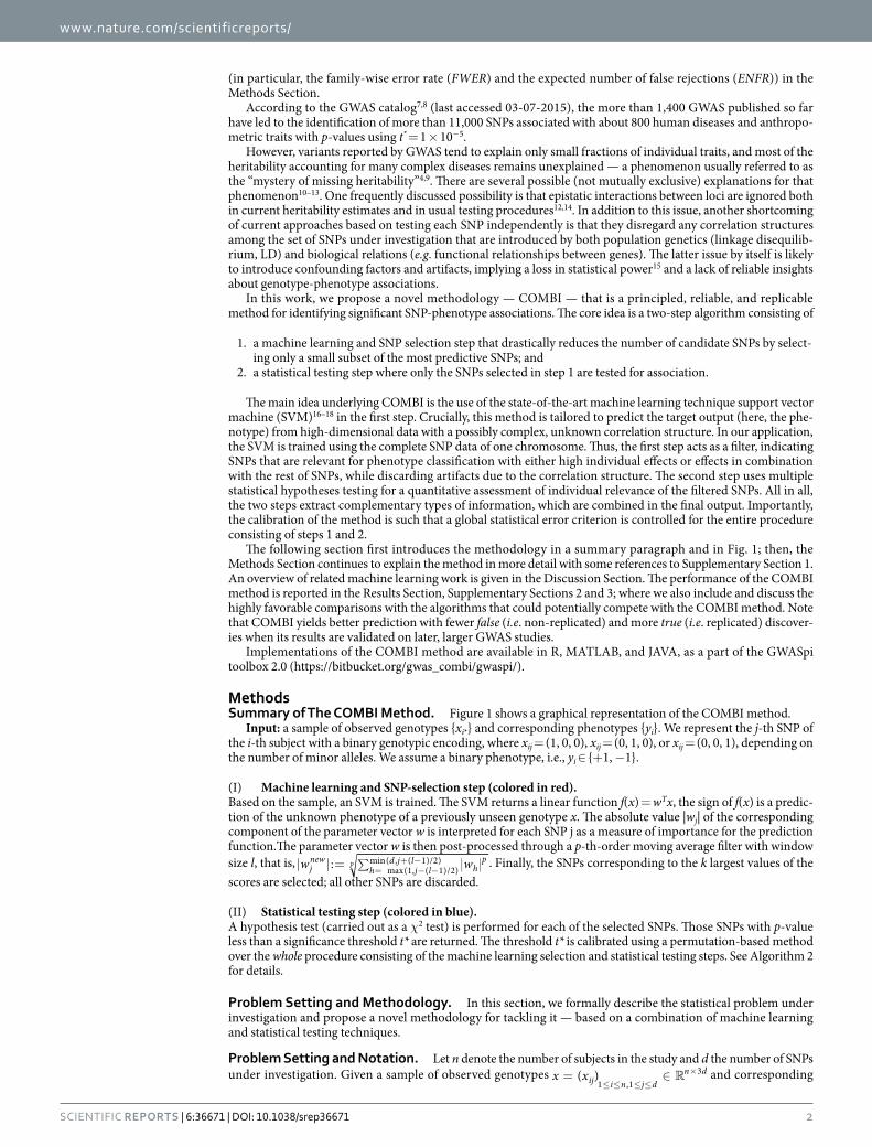
Validation using WTCCC data. We then compared the performance of the COMBI method to that of other methods when applied to data from the 2007 WTCCC phase 1, consisting of 14,000 cases of seven common diseases and 3,000 shared controls (see Supplementary Section 3 for further information). In contrast to the sim-ulations described above, the true underlying architecture of the traits under study is largely unknown. Hence, we used replicability in independent studies, one of the standards in the field, as a measure of performance. In summary, we proceeded as follows: the application of some method (for instance, COMBI or RPVT) to the 2007 WTCCC data results in a list of SNPs that are potentially associated with the trait (this is illustrated on the left-hand side of Fig. 2).

We then evaluated this list of potentially associated SNPs for replicability on independent data to obtain the “List of confirmed associated SNPs” (illustrated on the right-hand side of Fig. 2). All studies for the WTCCC diseases included in the GWAS catalog by June 26, 2015 constituted the set of studies examined for replicability. Most of these studies were performed either with larger sample sizes or using meta-analysis techniques and were published after the original WTCCC paper. In a sense, we thus examined how well any particular method, when applied to the WTCCC dataset, is able to make discoveries in that dataset that were actually confirmed by later research using RPVT in independent publications.

Our validation procedure considers a physical window of 200kb around a certain SNP and selects all SNPs with strong LD (R2 > 0.8) with the original SNP within that window. It queries the GWAS catalog for those SNPs to find out whether the selected SNPs have any entries. A hit indicates that a GWAS other than the original WTCCC study has since reported this SNP to be associated with the disease. Note that the GWAS catalog only contains SNPs with p-values < 10−5, meaning that we will miss some hits that are statistically weak but that might be biologically relevant, in the sense that they contribute to the classification of individuals according to phe-notypes. For a detailed description of the automatic validation procedure, see Supplementary Section 3.2. With this procedure, methods can be compared by counting the respective number of replicated and non-replicated reported associations.

Figure 2. Illustration of validation methodology. After producing a list of associated SNPs via an appropriate inference method (i.e. COMBI or RPVT), the GWAS catalog is used in an independent validation step to confirm or refute those candidate SNPs accessing the predictability of the used inference method.



Regarding significance levels, we aimed to stay as close in line with the original WTCCC study as possi-ble, reporting not only the strong associations at the significance level of 5 × 10−7 but also weak associations at 1 × 10−5. Within our validation pipeline we considered the full NHGRI GWAS Catalog7 with the inclusion criterion of having achieved a p-value of 1× 10−5 in a GWAS. The “somewhat liberal statistical threshold of p < 1 × 10−5 was chosen to allow examination of borderline associations and to accommodate scans of various sizes while maintaining a consistent approach”7.

We also ensured that the same statistical criterion (control of the FWER or the ENFR, respectively) was used for all methods, in order to have a fair comparison. This procedure is explained in detail in the Methods Section and Supplementary Section 1.1.1.

Stability analysis. In addition, we established an “internal” validation by analyzing the stability of the reported associations (cf. Supplementary Section 3.4 for details); this stability measure indicates how well results can be reproduced on another independent sample.

Parameter selection. The analysis of WTCCC data required the selection of all free parameters of the COMBI method (e.g. the SVM optimization parameter C, the window size l of the moving average filter or the filter norm parameter p). To this end, the semi-real datasets investigated in Supplementary Section 2 have been used to determine performance changes induced by varying those free parameters. Since our findings were in agreement with related literature and mostly biologically sensible, the optimal settings were assumed to be good choices for the application of the COMBI method to real data. For example, it was found that aggregating SNPs within the filtering step (See Summary of the COMBI method and Fig. 1, the filtering step) based on a filter size of 35 is optimal, which is on the same magnitude as in Alexander and Lange31 who find that grouping of SNPs into bins of size 40 helps the performance of their algorithm. The moving average filter of the COMBI method is designed to correct for non-independence of statistical tests within LD blocks. Given the SNP density in the arrays used by the original WTCCC study and LD patterns in the CEU population (1000 Genomes), we estimate that the average LD block (r2 > 0.8) will harbor no more than 20–30 SNPs32, which supports our findings of setting the filter window size to 35 in the sense that we average-out blocks and conservatively add a bit of noise by potentially smoothing out signals across blocks.

See Supplementary Section 1.1 for a detailed description of the selection of all free parameters of the COMBI method.

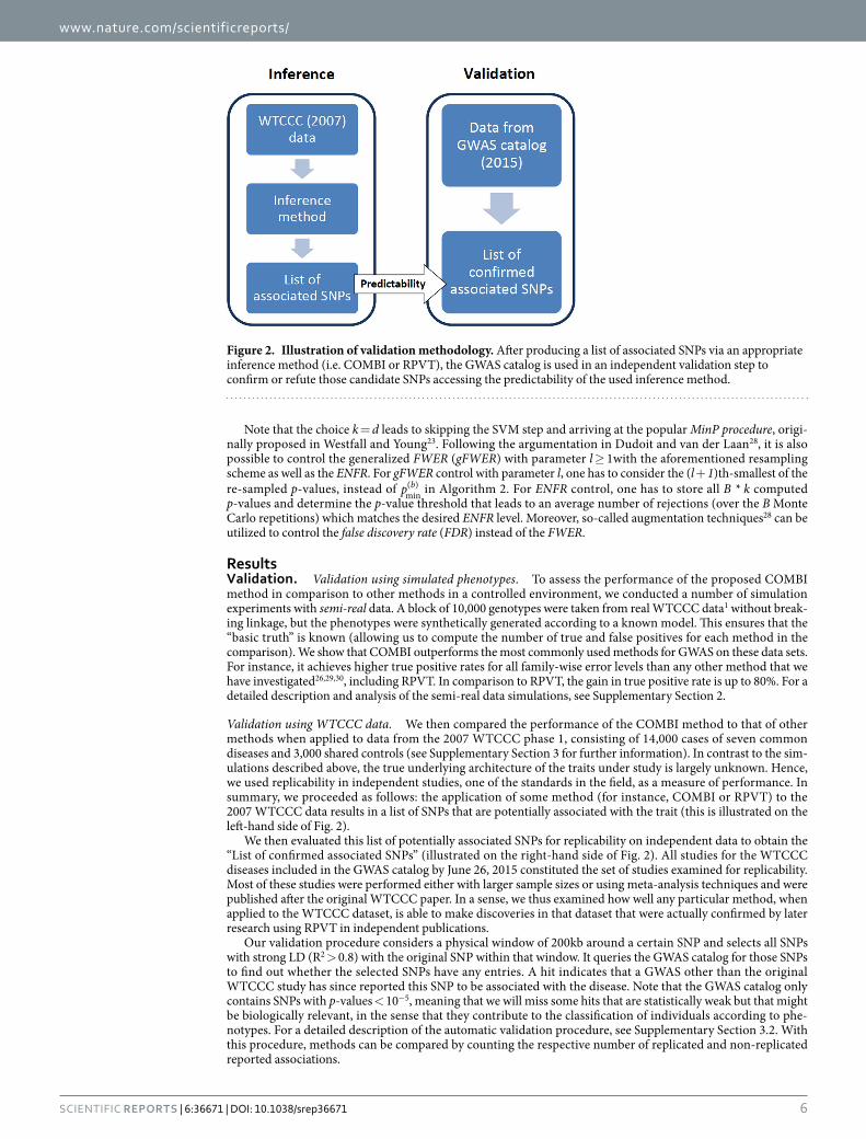
Figure 3. Genome-wide scan for seven diseases. Manhattan plots for all seven diseases resulting from the standard RPVT approach and the COMBI method as well as the SVM weights. We plot − log10 of the χ 2 trend test p-values for both COMBI and RPVT and the corresponding SVM weights against position on each chromosome. Chromosomes are shown in alternating colours for clarity, with significant p-values highlighted in green. Please note that for the RPVT, the threshold indicated by the horizontal dashed line is fixed a priori genome-wide. For the COMBI method, it was determined chromosome-wise via the permutation-based threshold over the whole COMBI procedure. All panels are truncated at − log10 (p-value) = 15, although some markers exceed this significance threshold.



Some parameters of the COMBI method could not be investigated within the simulation study, but had to be chosen manually for the WTCCC data. The decision to train the SVM separately on each chromosome was one of those tuning steps, as genome-wide training is very time and memory consuming on the one hand, and can only improve performance marginally on the other hand, as intergenic correlations between chromosomes are very rare.

Another parameter that was chosen manually was the number of active SNPs in one chromosome, i.e. the parameter k of The Screening Step presented in the Methods Section, which was set to 100 SNPs per chromosome after careful consideration. This choice is admittedly a wide, arbitrary upper bound for the number of SNPs that can present a detectable association with a given phenotype. Currently, the maximum total number of SNPs (not independent signals) associated with any phenotype is ~450 for human height and 180 for Crohn’s Disease (GWAS Catalog, accessed June 2015), so with k = 100 per chromosome one is well within what current evidence would support. After all, for future applications of COMBI k is a tuning parameter which has to be chosen by the researcher according to the assumed number of relevant loci.

The choice of exact values for all parameters will probably need to be adapted for each particular phenotype or disease under study, since they will have different genetic architectures and distribution of effect sizes4,9. For this manuscript and in order to provide a comprehensive and comparable set of results across many diseases we employed a unique set of parameter values supported by the results of our simulation study and other findings in related literature.

Manhattan plots and descriptive results. Figure 3 displays Manhattan plots for all seven diseases result-ing from the standard RPVT approach (left) and the COMBI method (center) as well as the SVM weights (right). The center and right graph illustrates that the COMBI method discards SNPs with a low SVM score (cf. “The screening step” in Summary of the COMBI method and Fig. 1). Hence, the p-values for such SNPs are set to one without performing a statistical test, thereby drastically reducing the number of candidate associations. In contrast, the RPVT method results in p-values based on a formal significance test for every SNP, where many of these p-values are small and produce a lot of statistical noise. SNPs that show genome-wide statistical sig-nificance are highlighted in green in the left and right panel. For the standard RPVT, the threshold indicated by the horizontal dashed line is fixed a priori genome-wide. For the COMBI method, however, it was deter-mined chromosome-wise via the permutation-based threshold over the whole COMBI procedure described in the Methods Section and Supplementary Section 1.1.1 to match the expected number of false rejections of RPVT.

In Table 2, we present all significant associations reported by the COMBI method. Associations with a raw p-value > 10−5 were not reported in studies using only RPVT. If they are selected by the COMBI method, we consider them to be new findings and highlight them in grey. The last column of Table 2 indicates whether the reported associations were validated (i.e., were reported as significant in at least one independent study published after the WTCCC). The COMBI method finds 46 significant locations. 34 of these 46 significant locations have a p-value below 10−5 and were thus also found by the RPVT approach.

Crucially, our COMBI method found 12 additional SNPs. Out of these, ten (> 83%) have already been rep-licated in later GWAS or meta analyses. The COMBI discoveries that have been replicated independently using individual SNP testing are for bipolar disorder rs2989476 (Chr. 1), rs1344484 (Chr. 16), rs4627791 (Chr. 3), and rs1375144 (Chr. 2); for coronary artery disease rs6907487 (Chr. 6) and rs383830 (Chr. 5); for Crohn’s disease rs12037606 (Chr. 1), rs10228407 (Chr. 7), and rs4263839 (Chr. 9) and for type 2 diabetes rs6718526 (Chr. 2). Given the current debate on the replicability of GWAS findings obtained by single-SNP analyses33, it is remarka-ble that GWAS studies published later had already replicated more than 83% of novel SNPs the COMBI method detected by reanalyzing data published in 2007.

Two out of the 12 SNPs with p-values exceeding 10−5 had not yet been reported in any GWAS or meta anal-yses as being associated with the corresponding diseases. Those are rs11110912 (Chr. 12) for hypertension and rs6950410 (Chr. 7) for type 1 diabetes. SNP rs11110912 was included in the original WTCCC analysis, but a p-value higher than 10−5 was obtained (1.94 × 10−5)1, so it was not collected in the GWAS Catalog. SNP rs6950410 has been detected as associated to multiple complex diseases34. Regarding the biological plausibility of these two SNPs, we examined a number of functional indicators to assess their potential role in disease. In particular, we explored the genomic regions in which they map and their potential roles as regulatory SNPs, status as eQTLs, and role in Mendelian disease. Overall, there is no strong evidence of functional roles (see Supplementary Section 3.5) but SNP rs11110912 (Chr. 12), for which COMBI suggested a link to hypertension, is an intronic SNP mapping on a gene, MYBPC1, that has been previously linked to familial hypertrophic cardiomyopathy, suggesting that COMBI has given rise to another interesting true positive finding.

GWAS catalog validation results – results obtained by the COMBI method are better replicated than those obtained by RPVT. The COMBI method also outperforms the RPVT approach for different type 1 error levels. Figure 4 shows the receiver operator characteristic (ROC) and precision-recall (PR) curves that have been generated based on the replication of SNPs according to the GWAS catalog (here, due to absence of basic truth knowledge, replicated reported associations are counted as true positives, and non-replicated asso-ciations as false positives). As the dark blue lines are consistently above the light blue lines, the COMBI method achieves both higher numbers of true positives (i.e. higher true positive rate (TPR)) as well as a higher precision (proportion of replicated associations amongst the SNPs classified as associated with the trait) for given numbers of false and true positives (i.e. lower false positive rate (FPR)) than RPVT for almost all levels of error. For com-parison, we show also the result achieved when selecting SNP based on the highest SVM weights in absolute value (after filtering). The results show that discarding either one of the two steps in the COMBI method (machine learning or statistical testing step) will lead to a decrease in performance.



We now investigate the points on the curves that correspond to the application of t* = 10−5 in the case of RPVT and to the value of t* resulting from the permutation-based method in the case of the COMBI method (described in the Methods Section) in more detail. See Table 3 for the numbers corresponding to those points.

Disease Chromosome Identifier χ2 p-valueSVM

weight

p-value < 10−5 in at least one external GWAS or

meta-analysis References (PMID)

Bipolar disorder (BD) 1 rs2989476 1.05e-05 0.0141 YES 19416921

2 rs1375144 1.26e-05 0.0146 YES 21254220

2 rs7570682 1.77e-06 0.0150 YES 21254220

3 rs4627791 1.18e-05 0.0150 YES 21254220

14 rs11622475 8.02e-06 0.0235 YES 21254220

16 rs1344484 1.10e-05 0.0245 YES 21254220

9 rs7860360 1.82e-06 0.0174

20 rs3761218 7.15e-06 0.0243 YES 21254220

Coronary artery disease 5 rs383830 1.35e-05 0.0174 YES 21804106

( CAD) 6 rs6907487 1.22e-05 0.0145 YES 17634449

9 rs1333049 1.12e-13 0.0262 YES 21606135

22 rs688034 2.75e-06 0.0287

Crohn’s disease (CD) 1 rs11805303 6.35e-12 0.0234

1 rs12037606 1.02e-05 0.0142 YES 17554261

2 rs10210302 4.52e-14 0.0224 YES 23128233

3 rs11718165 2.04e-08 0.0163 YES 21102463

5 rs6596075 3.11e-06 0.0168

5 rs17234657 2.42e-12 0.0305 YES 18587394

7 rs10228407 1.08e-05 0.0160

9 rs4263839 1.61e-05 0.0201 YES 21102463

10 rs10883371 5.23e-08 0.0227 YES 21102463

16 rs2076756 7.55e-15 0.0361 YES 21102463

18 rs2542151 1.93e-07 0.0246 YES 18587394

Hypertension (HT) 1 rs2820037 7.41e-07 0.0155

12 rs11110912 1.58e-05 0.0197

15 rs2398162 6.01e-06 0.0230

Rheumatoid arthritis 1 rs6679677 < 1.0e-15 0.0243 YES 20453842

(RA) 4 rs3816587 7.28e-06 0.0163

6 rs9272346 7.38e-14 0.0239

Type 1 diabetes (T1D) 1 rs6679677 < 1.0e-15 0.0247 YES 19430480

2 rs231726 1.43e-06 0.0129

4 rs17388568 3.07e-06 0.0175 YES 21829393

5 rs17166496 5.97e-06 0.0148

6 rs9272346 < 1.0e-15 0.0792 YES 18978792

7 rs6950410 1.03e-05 0.0172

12 rs17696736 1.55e-14 0.0223 YES 18978792

12 rs11171739 8.36e-11 0.0244 YES 19430480

16 rs12924729 7.86e-08 0.0285 YES 17554260

Type 2 diabetes (T2D) 2 rs6718526 1.00e-05 0.0159 YES 20418489

4 rs1481279 9.44e-06 0.0173

4 rs7659604 9.61e-06 0.0175

6 rs9465871 3.38e-07 0.0162

10 rs4506565 5.01e-12 0.0267 YES 23300278

12 rs1495377 7.21e-06 0.0196

16 rs7193144 4.15e-08 0.0293 YES 22693455

18 rs1025450 1.98e-06 0.0271

Table 2. Association analysis of the SNPs reaching genome-wide significance applying the COMBI method. For all seven diseases we present SNPs reaching genome-wide significance along with their rs-identifier, corresponding chromosome, χ 2 trend test p-value, SVM weight and the result of the validation pipeline indicating whether the SNP has been found significant with a p-value < 10−5 in at least one external GWAS or meta-analysis. PMID references of those studies are given in the last column. SNPs that do not show genome-wide significance in the case of RPVT are highlighted in bold case.


1 0Scientific RepoRts | 6:36671 | DOI: 10.1038/srep36671

A total of 78 SNPs were found to be significant with RPVT, since it only performs the statistical testing step, and 46 with the COMBI method, which has the additional layer of the machine learning screening step prior to the statistical testing.

Although the COMBI method finds fewer SNPs, the number of replicated SNPs is greater (28 in contrast to 24 of RPVT). The COMBI method also classifies only 18 of the unreplicated SNPs as associated with the trait (yield-ing a precision of 61%). This is in contrast to RPVT, which classifies 52 of the unreplicated SNPs as associated with the trait (yielding a precision of only 32%). In other words, if both methods are calibrated with respect to the same type I error criterion, the COMBI method reports significantly more replicated associations (Fisher’s exact test p-value of 0.0014).

Stability results – COMBI method is more stable than RPVT. From simulations considering internal stability, we found that the COMBI method produces more stable results than RPVT; cf. Supplementary Section 3.4 for details.

Runtime analysis and implementation details. The COMBI method is implemented in Matlab/Octave, R and Java as a part of the GWASpi toolbox 2.0 (https://bitbucket.org/gwas_combi/gwaspi/). The complete method is available in all these programming languages. The implementation for Matlab/Octave is cluster ori-ented and uses libLinear35. The Java implementation is desktop computer oriented and makes use of the following packages: libLinear35, libSVM36 and apache commons math37. Finally, the R implementation requires LiblineaR38, qqman39, data.table40, gtools41 and snpStats42.

Figure 4. ROC and PR curves of the RPVT approach, the COMBI method and raw SVM weights using the independent validation pipeline as an indicator of replicability. The results of all seven diseases have been pooled. The curves have been generated based on the replication of SNPs according to the GWAS catalog. Replicated reported associations are counted as true positives, and non-replicated associations as false positives. Note that the COMBI lines end at some point and the RPVT and the raw SVM lines continue. At the endpoint of the COMBI curve all SNPs selected in the SVM step are also significant in the statistical testing step; i.e. if one wanted to add just one more SNP to the list of reported associations, all other SNPs would also become significant, as they have a p-value of 1. The points on the RPVT and COMBI lines represent the final results of the two methods when applying the corresponding significance thresholds and are described in more detail in Table 3.

Number of SNPs reaching significance applying

RPVT COMBI Method

SNPs that have achieved < 10−5 in at least one external study 24 (32% precision) 28 (61% precision)

SNPs that have not achieved < 10−5 in an external study 52 (68% error) 18 (39% error)

Overall 76 46

p-value (one-sided Fisher’s exact test) 0.0014

Table 3. Empirical evaluation of the performance of the COMBI method on the WTCCC data, relative to that of basic RPVT. The table represents the information given by the points on the RPVT and COMBI lines in Fig. 4. The final results of the two methods when applying the corresponding significance thresholds are shown. At significance threshold t* = 10−5, COMBI achieves 28 SNPs recall at precision 61%, while RPVT achieves a recall of only 24 SNPs at precision 32%.

https://bitbucket.org/gwas_combi/gwaspi/



The runtime of the method depends on a variety of factors such as available cluster memory, hardware resources and operating system. For this analysis we have run the method with the Matlab/Octave implemen-tation on the following technical platform: 40 * Intel(R) Xeon(R) CPU E5-2650 v3 @ 2.30GHz 64bit, 128GB RAM, Ubuntu 14.04.4 LTS (GNU/Linux 3.13.0–79-generic x86_64), GNU Octave version 3.8.1. The analysis of WTCCC’s data on Crohn’s disease chromosome 18 (assuming calculations on more chromosomes can be com-puted in parallel if necessary) took 9h 15min and 24s. See Supplementary Section 3.7 for a more detailed runtime analysis.

DiscussionSeveral related machine learning methods have been successfully used in the context of statistical genomics. These approaches can be classified into two groups:

1. Methods that construct a model from genetic data in order to carry out accurate predictions on a phenotype43–56.2. Methods that use machine learning to construct a statistical association test or rank genetic markers according

to their predicted association with a phenotype30,31,57–67.

The set of papers that fall into the first category study the predictive performance of penalized regression and classification models including support vector machines16–18, random forests68, and sparsity-inducing methods such as the elastic net69 on various complex diseases (including the ones studied here), showing that machine learning methods such as SVMs – if appropriately applied - can perform well at predicting disease risks. See Supplementary Section 3.3, where we compare the prediction performance of various methods on the WTCCC data.

However, the main point of interest of the present contribution does not lie in risk prediction but rather in the identification of regions associated with diseases. The COMBI method should thus be compared to true alterna-tive methods that stem from the second category, some of which include two-stage approaches first performing statistical testing and then machine learning to refine the set of predicted associations30,57. These approaches, however, are unable to identify correlation structures of SNPs that have been excluded in the first step and neither method is validated on real data in terms of a comparison to the GWAS database. Similarly, Pahikkala et al.59 and He and Lin60 develop methods for ranking genetic markers based on the sure independence screening strategy70 and stability selection analyzing only one SNP at a time. Recently the approach has been extended to detect gene-to-gene interactions by Li et al.71, but neither of the methods have been validated on independent external studies.

Another approach is by Alexander and Lange31, who apply the stability selection method of Meinshausen and Bühlmann58 to the WTCCC data set to rank SNPs according to their predicted association with a phenotype. The authors find that stability selection effectively controls the FWER when applied to GWAS data but suffers a loss of power, while at the same time rendering conservative results.

The work that is probably most closely related to the present research is the two-step algorithm by Wasserman and Roeder27 (and the extension by Meinshausen et al.26), who split the data into two equal parts performing marker selection on the first part and then testing the selected markers on the second part. See Supplementary Section 2.2.4 for a detailed description of this approach.

In order to investigate and compare performance of the COMBI method to other machine learning approaches, the work of Roshan et al.30, Wasserman and Roeder27 and Meinshausen et al.26 are selected as repre-sentative baseline methods. In Supplementary Section 2.2.4, we show that the COMBI approach outperforms all of these methods on semi-real data.

An important and very closely related recent method by Lippert et al.14,72 aims to identify putative significant disease-marker associations using two approaches based on linear mixed models (LMMs): a univariate test and a test for pairwise epistatic interactions. LMMs, like COMBI, address the issue of population stratification in GWAS, cf. Mimno et al.73. However, in contrast to COMBI, they still test SNPs (or pairs of SNPs) individually one after the other and thus potentially lose detection power. Another possible shortcoming of LMMs and related methods over SVMs is that they are more tailored for regression and not binary classification. For a comparison of COMBI with Lippert et al.14,72 on real WTCCC data see Supplementary Section 3.6. Recently their approach has been extended for disease risk prediction (Rakitsch et al.56) and related approaches have been proposed by Loh et al.74 and Song et al.75 suffering the same drawbacks as discussed above.

An extension of LMMs to multivariate cases was developed by Zhou and Stephens76, but has not yet been applied to WTCCC. Fitting LMMs to multiple phenotypes provides no novel insight into analyzing multiple genotypes/SNPs at once, which is the issue COMBI addresses.

Our approach can be extended to explore a number of different research directions by substituting one of the two steps of the algorithm with other suitable procedures. Thus, one could either apply other machine learning prediction methods (as mentioned above) instead of training an SVM in the first step of the COMBI method. For example, the SVM training could be replaced by a SNP selection by random forests or component-wise boost-ing. Alternatively, one could perform a different statistical test in the final step of the COMBI method, such as procedures correcting for population structures or other confounding factors72,77. These alternatives are possible options for future research (and some have been implemented in the literature), however, COMBI performs bet-ter than any of the other machine learning methods we compared it to (Supplementary Section 2.2.4).

COMBI also seems to perform better than other state-of-the-art methods for univariate analyses. For instance, a recent method by Lippert et al.14 aims to identify putative significant disease-marker associations from the WTCCC data using two approaches based on linear mixed models: an univariate test and a test for pairwise epistatic interactions. When their univariate method results are checked against the same validation criteria that



we used for COMBI, it turns out that our method reports 17 more true positives (4.4 times more positives) for the three diseases for which their univariate method reports at least one hit (Supplementary Section 3.6).

The COMBI method also holds great potential for testing pairwise SNP-trait associations, as it drastically reduces the number of candidate associations by selecting a subset of the most predictive SNPs in the machine learning step. Again, a comparison against the method Lippert et al.14 propose for detecting epistatic interactions, is favorable to COMBI (see Supplementary Section 3.6). In future work we will extend the COMBI method to a regression setup where the phenotype is not binary.

To summarize, we proposed a novel and powerful method for analyzing GWAS data that is based on applying a carefully designed machine learning step that is tailored to the GWAS data before applying a classical mul-tiple testing step. Certain machine learning models, in particular appropriately designed linear SVMs, take high-dimensional correlation structures into account and thus implicitly incorporate interactions between dif-ferent loci. A subset of predictive candidate SNPs is extracted within the machine learning step. The p-values corresponding to association tests are then thresholded for these candidate SNPs in a subsequent statistical test-ing step. The COMBI method was shown to outperform the RPVT approach both on controlled, semi-real data and on data from the WTCCC 2007 study, for which reported associations were validated by their replicability in external later studies. The empirical analysis showed a significant increase in detection power for replicated SNPs, while yielding fewer unconfirmed discoveries. Two new (as yet unreplicated) candidate associations were reported.

References1. The Wellcome Trust Case Control Consortium. Genome-wide association study of 14,000 cases of seven common diseases and

3,000 shared controls. Nature 447, 661–678 (2007).2. Wray, N. R. et al. Pitfalls of predicting complex traits from SNPs. Nat. Rev. Genet. 14, 507–515 (2013).3. Edwards, S. L., Beesley, J., French, J. D. & Dunning, A. M. Beyond GWASs: illuminating the dark road from association to function.

Am. J. Hum. Genet. 93, 779–797 (2013).4. Visscher, P. M., Brown, M. A., McCarthy, M. I. & Yang, J. Five years of GWAS discovery. Am. J. Hum. Genet. 90, 7–24 (2012).5. Ripke, S. et al. Genome-wide association analysis identifies 13 new risk loci for schizophrenia. Nat. Genet. 45, 1150–1159 (2013).6. Beecham, A. H. et al. Analysis of immune-related loci identifies 48 new susceptibility variants for multiple sclerosis. Nat. Genet. 45,

1353–1360 (2013).7. Hindorff, L. A. et al. Potential etiologic and functional implications of genome-wide association loci for human diseases and traits.

Proc. Natl. Acad. Sci. 106, 9362–9367 Catalog of Published Genome-Wide Association Studies at www.genome.gov/gwastudies (2009).

8. Welter, D. et al. The NHGRI GWAS Catalog, a curated resource of SNP-trait associations. Nucleic Acids Res. 42, D1001–D1006 (2014).

9. Manolio, T. a. et al. Finding the missing heritability of complex diseases. Nature 461, 747–753 (2009).10. Lee, S. H., Wray, N. R., Goddard, M. E. & Visscher, P. M. Estimating missing heritability for disease from genome-wide association

studies. Am. J. Hum. Genet. 88, 294–305 (2011).11. Gibson, G. Rare and common variants: twenty arguments. Nat. Rev. Genet. 13, 135–145 (2012).12. Zuk, O., Hechter, E., Sunyaev, S. R. & Lander, E. S. The mystery of missing heritability: Genetic interactions create phantom

heritability. Proc. Natl. Acad. Sci. 109, 1193–1198 (2012).13. Mackay, T. F. C. Epistasis and quantitative traits: using model organisms to study gene-gene interactions. Nat. Rev. Genet. 15, 22–33

(2014).14. Lippert, C. et al. An exhaustive epistatic SNP association analysis on expanded Wellcome Trust data. Sci. Rep. 3, 1099 (2013).15. Van de Geer, S., Bühlmann, P., Ritov, Y. & Dezeure, R. On asymptotically optimal confidence regions and tests for high-dimensional

models. Ann. Stat. 42, 1166–1202 (2014).16. Boser, B. E., Guyon, I. M. & Vapnik, V. N. A Training Algorithm for Optimal Margin Classifiers. In Fifth Annual Workshop on

Computational Learning Theory 144–152 (ACM Press, 1992).17. Cortes, C. & Vapnik, V. Support-vector networks. Mach. Learn. 20, 273–297 (1995).18. Müller, K. R., Mika, S., Rätsch, G., Tsuda, K. & Schölkopf, B. An introduction to kernel-based learning algorithms. IEEE Trans.

neural networks 12, 181–201 (2001).19. Agresti, A. Categorical Data Analysis. (Wiley, 2002).20. Moskvina, V. & Schmidt, K. M. On multiple-testing correction in genome-wide association studies. Genet. Epidemiol. 32, 567–573

(2008).21. Dickhaus, T. & Stange, J. Multiple point hypothesis test problems and effective numbers of tests for control of the family-wise error

rate. Calcutta Stat. Assoc. Bull. 65, 123–144 (2013).22. Dickhaus, T. Simultaneous Statistical Inference with Applications in the Life Sciences. (Springer, 2014).23. Westfall, P. & Young, S. Resampling-Based Multiple Testing: Examples and Methods for p-Value Adjustment. (Wiley, 1993).24. Meinshausen, N., Maathuis, M. H. & Bühlmann, P. Asymptotic optimality of the Westfall-Young permutation procedure for multiple

testing under dependence. Ann. Stat. 39, 3369–3391 (2011).25. Guyon, I. & Elisseeff, A. An introduction to variable and feature selection. Journal of machine learning research 3, 1157–1182

(2003).26. Meinshausen, N., Meier, L. & Bühlmann, P. p-Values for High-Dimensional Regression. J. Am. Stat. Assoc. 104, 1671 (2009).27. Wasserman, L. & Roeder, K. High-dimensional variable selection. Ann. Stat. 37, 2178–2201 (2009).28. Dudoit, S. & van der Laan, M. Multiple Testing Procedures with Applications to Genomics. (Springer Science & Business Media,

2008).29. Roeder, K. & Wasserman, L. Genome-Wide Significance Levels and Weighted Hypothesis Testing. Stat. Sci. 24, 398–413

(2009).30. Roshan, U., Chikkagoudar, S., Wei, Z., Wang, K. & Hakonarson, H. Ranking causal variants and associated regions in genome-wide

association studies by the support vector machine and random forest. Nucleic Acids Res. 39, e62 (2011).31. Alexander, D. H. & Lange, K. Stability selection for genome-wide association. Genet. Epidemiol. 35, 722–728 (2011).32. The HapMap International Consortium. A haplotype map of the human genome. Nature 437, 1299–1320 (2005).33. Marigorta, U. M. & Navarro, A. High Trans-ethnic Replicability of GWAS Results Implies Common Causal Variants. PLoS Genet 9,

e1003566 (2013).34. Preuss, C., Riemenschneider, M., Wiedmann, D. & Stoll, M. Evolutionary dynamics of co-segregating gene clusters associated with

complex diseases. PLoS One 7, e36205 (2012).35. Fan, R.-E., Chang, K.-W., Hsieh, C.-J., Wang, X.-R. & Lin, C.-J. LIBLINEAR: A Library for Large Linear Classification. Journal of

Machine Learning Research 9, 1871–1874. Software available at http://www.csie.ntu.edu.tw/~cjlin/liblinear (2008).

http://www.genome.gov/gwastudies

http://www.csie.ntu.edu.tw/~cjlin/liblinear



36. Chang, C.-C. & Lin, C.-L. LIBSVM: a library for support vector machines. ACM Trans. Intell. Syst. Technol. 2(27), 1–27. Software available at http://www.csie.ntu.edu.tw/~cjlin/libsvm (2011).

37. The Apache Software Foundation. Commons Math: The Apache Commons Mathematics Library. Java version 1.7. Software available at http://commons.apache.org/proper/commons-math/ (2016).

38. Helleputte, T. & Gramme, P. LiblineaR: Linear Predictive Models Based on the LIBLINEAR C/C+ + Library. R package version 1.94-2 from http://dnalytics.com/liblinear/ (2015).

39. Turner, S. D. qqman: an R package for visualizing GWAS results using Q-Q and manhattan plots. biorXiv doi: 10.1101/005165. R package version 0.1.2 from http://cran.r-project.org/web/packages/qqman/ (2014).

40. Dowle, M., Srinivasan, A., Short, T. & Lianoglou, S. with contributions from Saporta, R. & Antonyan, E. data.table: Extension of Data.frame. R package version 1.9.6. from https://CRAN.R-project.org/package= data.table (2015).

41. Warnes, G. R., Bolker, B. & Lumley, T. gtools: Various R Programming Tools. R package version 3.5.0. from https://CRAN.R-project.org/package= gtools (2015).

42. Clayton, D. snpStats: SnpMatrix and XSnpMatrix classes and methods. R package version 1.22.0 from http://bioconductor.org/packages/release/bioc/html/snpStats.html (2015).

43. Mittag, F. et al. Use of support vector machines for disease risk prediction in genome-wide association studies: Concerns and opportunities. Hum. Mutat. 33, 1708–1718 (2012).

44. Davies, R. W. et al. Improved Prediction of Cardiovascular Disease Based on a Panel of Single Nucleotide Polymorphisms Identified Through Genome-Wide Association Studies. Circ. Cardiovasc. Genet. 3, 468–474 (2010).

45. Evans, D. M., Visscher, P. M. & Wray, N. R. Harnessing the information contained within genome-wide association studies to improve individual prediction of complex disease risk. Hum. Mol. Genet. 18, 3525–3531 (2009).

46. Ioannidis, J. P. A. Prediction of Cardiovascular Disease Outcomes and Established Cardiovascular Risk Factors by Genome-Wide Association Markers. Circ. Cardiovasc. Genet. 2, 7–15 (2009).

47. Kooperberg, C., LeBlanc, M. & Obenchain, V. Risk prediction using genome-wide association studies. Genet. Epidemiol. 34, 643–652 (2010).

48. Quevedo, J. R., Bahamonde, A., Perez-Enciso, M. & Luaces, O. Disease Liability Prediction from Large Scale Genotyping Data Using Classifiers with a Reject Option. IEEE/ACM Trans. Comput. Biol. Bioinforma. 9, 88–97 (2012).

49. Wei, Z. et al. From Disease Association to Risk Assessment: An Optimistic View from Genome-Wide Association Studies on Type 1 Diabetes. PLoS Genet. 5, e1000678 (2009).

50. Wei, Z. et al. Large Sample Size, Wide Variant Spectrum, and Advanced Machine-Learning Technique Boost Risk Prediction for Inflammatory Bowel Disease. Am. J. Hum. Genet. 92, 1008–1012 (2013).

51. Wray, N. R., Yang, J., Goddard, M. E. & Visscher, P. M. The genetic interpretation of area under the ROC curve in genomic profiling. PLoS Genet. 6, e1000864 (2010).

52. Austin, E., Pan, W. & Shen, X. Penalized regression and risk prediction in genome-wide association studies. Stat. Anal. Data Min. 6, 315–328 (2013).

53. Okser, S. et al. Regularized machine learning in the genetic prediction of complex traits. PLoS Genet. 10, e1004754 (2014).54. Wu, Q., Ye, Y., Liu, Y. & Ng, M. K. SNP selection and classification of genome-wide SNP data using stratified sampling random

forests. IEEE Trans. Nanobiosci. 11, 216–227 (2012).55. Schwarz, D. F., König, I. R. & Ziegler, A. On safari to Random Jungle: a fast implementation of Random Forests for high-dimensional

data. Bioinformatics 26, 1752–1758 (2010).56. Rakitsch, B., Lippert, C., Stegle, O. & Borgwardt, K. A Lasso multi-marker mixed model for association mapping with population

structure correction. Bioinformatics 29, 206–214 (2013).57. Shi, G. et al. Mining gold dust under the genome wide significance level: a two-stage approach to analysis of GWAS. Genet.

Epidemiol. 35, 111–118 (2011).58. Meinshausen, N. & Bühlmann, P. Stability selection. J. R. Stat. Soc. Ser. B Statistical Methodol. 72, 417–473 (2010).59. Pahikkala, T., Okser, S., Airola, A., Salakoski, T. & Aittokallio, T. Wrapper-based selection of genetic features in genome-wide

association studies through fast matrix operations. Algorithms Mol. Biol. 7, 11 (2012).60. He, Q. & Lin, D. Y. Y. A variable selection method for genome-wide association studies. Bioinformatics 27, 1–8 (2011).61. Zhou, H., Sehl, M. E., Sinsheimer, J. S. & Lange, K. Association screening of common and rare genetic variants by penalized

regression. Bioinformatics 26, 2375–2382 (2010).62. Minnier, J., Yuan, M., Liu, J. S. & Cai, T. Risk classification with an adaptive naive Bayes Kernel machine model. J. Am. Stat. Assoc.

110, 393–404 (2015).63. Nguyen, T. T., Huang, J. Z., Wu, Q., Nguyen, T. T. & Li, M. J. Genome-wide association data classification and SNPs selection using

two-stage quality-based Random Forests. BMC Genomics 16, S5 (2015).64. Tsai, M. Y. Variable selection in Bayesian generalized linear-mixed models: An illustration using candidate gene case-control

association studies. Biometrical Journal 57, 234–253 (2015).65. Manor, O. & Segal, E. Predicting disease risk using bootstrap ranking and classification algorithms. PLoS Comput. Biol. 9, e1003200

(2013).66. Hoffman, G. E., Logsdon, B. A. & Mezey, J. G. PUMA: a unified framework for penalized multiple regression analysis of GWAS data.

PLoS Comput. Biol. 9, e1003101 (2013).67. Fisher, C. K. & Mehta, P. Bayesian feature selection for high-dimensional linear regression via the Ising approximation with

applications to genomics. Bioinformatics 11, 1754–1761 (2015).68. Breiman, L. Random forests. Machine learning 45, 5–32 (2001).69. Zou, H. & Hastie, T. Regularization and variable selection via the elastic net. J. R. Stat. Soc. Ser. B Statistical Methodol. 67, 301–320

(2005).70. Fan, J. & Lv, J. Sure independence screening for ultrahigh dimensional feature space. J. R. Stat. Soc. Ser. B Statistical Methodol. 70,

849–911 (2008).71. Li, J., Zhong, W., Li, R. & Wu, R. A fast algorithm for detecting gene–gene interactions in genome-wide association studies. The

annals of applied statistics 8, 2292 (2014).72. Lippert, C. et al. FaST linear mixed models for genome-wide association studies. Nat. Methods 8, 833–835 (2011).73. Mimno, D., Blei, D. M. & Engelhardt, B. E. Posterior predictive checks to quantify lack-of-fit in admixture models of latent

population structure. Proc. Natl. Acad. Sci. 112, 3441–3450 (2015).74. Loh, P. R. et al. Efficient Bayesian mixed-model analysis increases association power in large cohorts. Nat. Genet. 47, 284–290

(2015).75. Song, M., Hao, W. & Storey, J. D. Testing for genetic associations in arbitrarily structured populations. Nat. Genet. 47, 550–554

(2015).76. Zhou, X. & Stephens, M. Efficient multivariate linear mixed model algorithms for genome-wide association studies. Nat. Methods

11, 407–409 (2014).77. Kang, H. M. et al. Efficient control of population structure in model organism association mapping. Genetics 178, 1709–1723

(2008).

http://www.csie.ntu.edu.tw/~cjlin/libsvm

http://commons.apache.org/proper/commons-math/

http://dnalytics.com/liblinear/

http://cran.r-project.org/web/packages/qqman/

https://CRAN.R-project.org/package=data.table

https://CRAN.R-project.org/package=gtools

https://CRAN.R-project.org/package=gtools

http://bioconductor.org/packages/release/bioc/html/snpStats.html

http://bioconductor.org/packages/release/bioc/html/snpStats.html



AcknowledgementsThis paper is part of a larger project on the genetics of social and economic behavior. The idea for this paper arose in the workshop that regularly takes place in the context of this project at the University of Zurich, and which is based on the collaboration of teams at universities in Berlin, Barcelona, Mainz, and Zurich. EF acknowledges support from the advanced ERC grant (ERC-2011-AdG 295642-FEP) on the Foundation of Economic Preferences. MK, BM, and KRM were supported by the German National Science Foundation (DFG) under the grants MU 987/6-1 and RA 1894/1-1. TD and DS were supported by the German National Science Foundation (DFG) under the grants DI 1723/3-1 und SCHU 2828/2-1. GB and TS acknowledge support of the German National Science Foundation (DFG) under the research group grant FOR 1735. MK, DT, KRM, and GB acknowledge financial support by the FP7-ICT Programme of the European Community, under the PASCAL2 Network of Excellence. MK acknowledges a postdoctoral fellowship by the German Research Foundation (DFG), award KL 2698/2-1, and from the Federal Ministry of Science and Education (BMBF) awards 031L0023A and 031B0187B. AN acknowledges support from the Spanish Multiple Sclerosis Network (REEM), of the Instituto de Salud Carlos III (RD12/0032/0011), the Spanish National Institute for Bioinformatics (PT13/0001/0026) the Spanish Government Grant BFU2012-38236 and from FEDER. This project has received funding from the European Union’s Horizon 2020 research and innovation programme under grant agreement No. 634143 (MedBioinformatics). MK and KRM were financially supported by the Ministry of Education, Science, and Technology, through the National Research Foundation of Korea under Grant R31-10008 (MK, KRM) and BK21 (KRM).

Author ContributionsE.F., T.D., G.B., D.S., A.N. and K.-R.M. designed and directed research; B.M., M.K., J.A.R., S.S., R.V., C M.-S., X.F., U.M.M. and D.S. performed research and analyzed data; and B.M., M.K., J.A.R., C M.-S., E.F., T.D., G.B., D.S., A.N. and K.-R.M. wrote the paper.

Additional InformationSupplementary information accompanies this paper at http://www.nature.com/srepCompeting financial interests: The authors declare no competing financial interests.How to cite this article: Mieth, B. et al. Combining Multiple Hypothesis Testing with Machine Learning Increases the Statistical Power of Genome -wide Association Studies. Sci. Rep. 6, 36671; doi: 10.1038/srep36671 (2016).Publisher's note: Springer Nature remains neutral with regard to jurisdictional claims in published maps and institutional affiliations.

This work is licensed under a Creative Commons Attribution 4.0 International License. The images or other third party material in this article are included in the article’s Creative Commons license,

unless indicated otherwise in the credit line; if the material is not included under the Creative Commons license, users will need to obtain permission from the license holder to reproduce the material. To view a copy of this license, visit http://creativecommons.org/licenses/by/4.0/ © The Author(s) 2016

http://www.nature.com/srep

http://creativecommons.org/licenses/by/4.0/

1

Supplementary Material

Combining Multiple Hypothesis Testing with Machine Learning

Increases the Statistical Power of Genome-wide Association Studies

Bettina Mieth, Marius Kloft, Juan Antonio Rodriguez, Sören Sonnenburg, Robin Vobruba,

Carlos Morcillo-Suarez, Xavier Farre, Urko M. Marigorta, Ernst Fehr, Thorsten Dickhaus,

Gilles Blanchard, Daniel Schunk, Arcadi Navarro & Klaus-Robert Müller

Content of supplementary material

1. Supplementary Methods

1.1. Parameter Selection

1.1.1. Determination of type 1 error level 𝜶

1.1.2. Other free parameters

1.2. Comparing SVM weights with RPVT p-values

2. Simulation study on controlled phenotypes

2.1. Simulation data

2.2. Results

2.2.1. COMBI method vs. standard RPVT

2.2.2. Conservativeness of the FWER control

2.2.3. Further experiments

2.2.4. Comparison to other state of the art methods

3. Analysis of real data (WTCCC, 2007)

3.1. Data preparation

3.2. Automatic validation procedure

3.3. Prediction performance

3.4. Stability analysis

3.5. Functional study of two non-replicated SNPs

3.6. Comparison to Fast-LMM models

3.7. Runtime analysis and implementation details

References of supplementary material

2

1. Supplementary Methods

1.1. Parameter Selection

1.1.1. Determination of type 1 error level 𝜶

Here, we discuss how to determine the type 1 error level α to be used in Algorithms 1 and 2

presented in the Methods Section of the main text when applying the COMBI method to the

WTCCC data1. When comparing the performance of the COMBI method with that of RPVT, α

should correspond to the error level applied in the original WTCCC study1. In that case, t* =

5*10-7 was determined to be a reasonable threshold for type 1 error control in RPVT stating

that, “the posterior odds in favor of a ‘hit’ being a true association would be 10:1” using this

threshold1. A sound upper bound on the expected number of false rejections (ENFR) level that

this threshold implies is obtained by calculating the empirical distribution of p-values using the

Westfall-Young2 procedure. It turned out that the threshold of t* = 5*10-7 will, on average,

produce 0.17 non-replicated discoveries per disease, or 1.19 for all seven. Out of the 24 SNPs

reported in WTCCC at t* = 5*10-7, only one can be expected to be a false positive, which

corresponds to a true-to-false-positives ratio of 23:1.

WTCCC also reported SNPs at the level t* = 10-5, stating that “if we relax the significance

threshold by a factor of ten […], the posterior odds that a ‘hit’ is a true association would also

be reduced by a factor of ten.”1 The relaxed threshold of 10-5 would thus refer to posterior odds

of 1:2. According to our simulations, the controlled number of non-replicated discoveries to be

expected is 3.32 per disease on average. This suggests that out of the 82 loci reported by the

WTCCC at t* = 10-5, we can expect that approximately 23 are false positives, corresponding to

an actual rate of true-to-false-positives of ~ 3:1.

To compare the performance of the COMBI method with that of RPVT in a fair way, we

consequently calibrated the COMBI method (using the Westfall and Young-type procedure

described in Algorithm 2 presented in the Methods Section of the main text) in a way such

that the number of non-replicated discoveries is bounded by 3.32 per disease (using the

3

augmentation for ENFR control of both algorithms). It should be noted that, when investigating

the performance of the COMBI method with semi-real data simulations, we observed that the

COMBI method produces only approximately 20% of the number of type 1 errors one is aiming

to control for (See Supplementary Section 2.2.2.). Although it is not known whether this

relation is true in the case of real data, we could expect still substantially fewer errors than what

the calibration aims for, i.e., around 0.664 instead of 3.32 per disease, if the data-generating

distribution is as in the simulations.

1.1.2. Other free parameters

In this section, we discuss how we chose the values of the free parameters of the COMBI

method for the investigation of the WTCCC data presented in the Methods Section of the main

text. To this end, the semi-real datasets investigated in Supplementary Section 2. where used

to determine performance changes induced by varying the free parameters of the COMBI

method. The optimal settings were assumed to be good choices for the application of the

COMBI method to real data.

As described in Problem Setting and Notation in the Methods Section of the main text, the

genotypic feature encoding method was applied, where all features where normalized such that

the 6th centered moments were all one (this is similar to the common practice of scaling each

feature to unit standard deviation).

As we can see from Equation 1 in The machine learning step in the Methods Section of the

main text, there are a number of parameters to be determined in the training of an SVM. During

the simulation experiments on the semi-real data sets, the value of the parameter C was

computed by internal cross-validation, in order to maximize the (estimated) generalization

ability of the function f. We found no significant effect of this parameter on the performance of

the COMBI method. We thus applied a fixed C = 0.00001 for the investigation of the real data,

economizing computation time and memory space. A linear L2 regularized L1-loss dual

4

classifier was applied3 to solve the SVM minimization problem. We trained the SVM on each

chromosome separately, as genome-wide training is very time and memory consuming on the

one hand, and can only improve performance marginally on the other hand, as intergenic

correlations between chromosomes are very rare.

Reasonable choices of the free parameters of Equation 3 in the filtering and screening step in

the Methods Section of the main text were shown to be optimal in the simulation experiments.

The window size l of the moving average filter was set to 35, which is in agreement with the

results of Alexander and Lange4, who investigated similar associations. The norm parameter p

of the filter was set to 2.

A reasonable upper bound for the number of active SNPs in one chromosome was found to be

100, which is why the parameter k of The Screening Step presented in the Methods Section

of the main text was set to this value.

The simulation experiments also showed better performance when the χ2 test for trend was

applied instead of the Cochran-Armitage test in The Statistical Testing Step presented in the

Methods Section of the main text.

1.2. Comparing SVM weights with RPVT p-values

A legitimate concern of readers could be that, even if Steps 1 and 2 of COMBI are run

independently of each other – in the sense that the w value of a SNP is obtained irrespectively

of what the p-value of the same SNP would be in a trend test performed under the usual

univariate RPVT setup – high correlations between w and p-values might still occur. If this was

the case, the statistical testing step in the COMBI procedure might have to use a more stringent

Bonferroni correction. Supplementary Fig. S1 and S2 below show that w and the

corresponding p-values are not highly correlated. While it is clear that COMBI hits tend to be

located in the area with high w values, note that several highly significant SNPs reported in the

5

WTCCC have moderate w values and, vice versa, that not all SNPs with high w turn out to be

significant. This was expected, since COMBI produces a simultaneous analysis of all SNPs,

rather than considering each SNP in isolation.

Supplementary Figure S1

Relation between SVM weights and p-values for all 444K SNPs for all seven diseases

studied. Following a general trend, higher weights tend to have more significant p-values.

However, clear cases with medium or lower weights also turn to be significant, pointing towards

the need of a full combined approach (SVM + p-value thresholding step)

6


Scatter plot of p-values (on –log scale) vs. SVM weights, least-squares regression line, and

R2. As in the former figure, there is a general trend of higher weights having more significant

p-values, but there are also many exceptions.

To analyze whether SNPs with high w values could be selected as potential hits (thus removing

the need of the 2nd step in the COMBI method), we took the top 2,000 SNPs with highest

weights and selected a single representative SNP for each of the loci included in the top weights

list. We obtained sets of SNPs of the following sizes for each disease: BD (n=115), CAD (117),

CD (n=96), Hypertension (103), Rheumatoid Arthritis (106), T1D (85) and T2D (114). We

excluded hits already reported by the full COMBI approach (those in Table 2 in the Main Text).

All of these sets were evaluated using the validation pipeline and precision-recall and ROC

curves can be seen in Figure 4 of the main text.

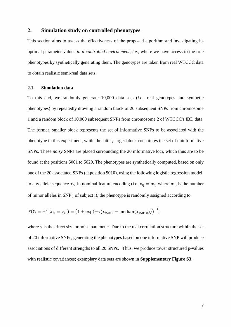
7

2. Simulation study on controlled phenotypes

This section aims to assess the effectiveness of the proposed algorithm and investigating its

optimal parameter values in a controlled environment, i.e., where we have access to the true

phenotypes by synthetically generating them. The genotypes are taken from real WTCCC data

to obtain realistic semi-real data sets.

2.1. Simulation data

To this end, we randomly generate 10,000 data sets (i.e., real genotypes and synthetic

phenotypes) by repeatedly drawing a random block of 20 subsequent SNPs from chromosome

1 and a random block of 10,000 subsequent SNPs from chromosome 2 of WTCCC's IBD data.

The former, smaller block represents the set of informative SNPs to be associated with the

phenotype in this experiment, while the latter, larger block constitutes the set of uninformative

SNPs. These noisy SNPs are placed surrounding the 20 informative loci, which thus are to be

found at the positions 5001 to 5020. The phenotypes are synthetically computed, based on only

one of the 20 associated SNPs (at position 5010), using the following logistic regression model:

to any allele sequence 𝑥𝑖∗ in nominal feature encoding (i.e. xij = mij where mij is the number

of minor alleles in SNP j of subject i), the phenotype is randomly assigned according to

ℙ(𝑌𝑖 = +1|𝑋𝑖∗ = 𝑥𝑖∗) = (1 + exp(−γ(𝑥𝑖5010 − median(𝑥∗5010)))−1

,

where γ is the effect size or noise parameter. Due to the real correlation structure within the set

of 20 informative SNPs, generating the phenotypes based on one informative SNP will produce

associations of different strengths to all 20 SNPs. Thus, we produce tower structured p-values

with realistic covariances; exemplary data sets are shown in Supplementary Figure S3.

8


p-values of several exemplary semi-real data sets. Note the tower structure induced by the 20

informative SNPs located at the positions 5001 to 5020. While the data sets (a), (b), and (d)

present quite strong associations, data set (c) only shows rather minor ones - this is a result of

the randomness involved in the generation process.

Note that the associations between the informative SNPs and the labels vary a lot in strength

due to the randomness in the generation process, which increases similarity to real genome data

sets.

The process of drawing random genotypes and generating the corresponding phenotypes is

repeated 10,000 times to generate 10,000 data sets.

An additive heritability model was assumed appropriate for this simulation study for a number

of different reasons. Most importantly it is the standard model in the field of SNP effect

estimation, genome risk score computation and other related problems5,6. This is especially true

for the seven diseases that are studied in this work. In the original WTCCC study, they used an

additive test as the null model, spotting only a few cases were departure from this additivity

was observed1. Additive, infinitesimal models have been shown to work well in the research

area of quantitative genetics and, indeed, most GWAS hits seem to behave additively7,8,9. It is

9

also the most agnostic model, with less parameters and no need to make any assumptions on

values of dominance or complex interactions between loci5,6. The investigation of other models

for the genetic architecture of a disease could be the subject of future research projects.

2.2. Results

In the following, we report results averaged over the 10,000 data sets realized by the Monte

Carlo simulation described above. The proposed COMBI method is compared to the standard

RPVT procedure using a Westfall-Young correction as well as the approach of Meinshausen et

al.10 (which itself is an extension of the method of Wasserman and Roeder11). As evaluation

criteria, we report the family-wise error rate, FWER, the expected number of false rejections,

ENFR, and the true-positive rate, TPR. The results are presented in the following section.

2.2.1. COMBI method vs. standard RPVT

The identification of SNPs that have an influence on the probability of having a positive label

in the semi-real data sets can be improved by applying the COMBI method, which achieves

significantly better results than the ordinary RPVT approach. The superiority of the new method

is displayed in Supplementary Figure S4, where we compare the power, as measured by the

TPR (averaged over the 10,000 runs) of the COMBI method to that achieved using the standard

RPVT procedure. Those rates can be determined for various levels of FWER (shown on the

left) and ENFR (shown on the right), respectively. It is obvious that the COMBI method

achieves greater power for all levels of FWER and ENFR, which is based on the fact that the

selection step of the COMBI method correctly filters out most of the noise SNPs and identifies

the informative SNPs accurately.

10


Main results of both COMBI and RPVT method applied to the simulated data sets with

controlled phenotypes: (a) TPR averaged over 10,000 synthetic data sets as a function of the

FWER. (b) TPR averaged over 10,000 synthetic data sets as a function of ENFR. (c) Precision-

Recall curves. (d) ROC curve. The dark blue lines (representing the COMBI method) are

uniformly above the light blue ones (representing RPVT) in all plots. The COMBI method thus

achieves higher TPR (i.e., multiple power) for all levels of FWER and ENFR. The dots in (a)

mark measurements of the permutation-based calibration where the corresponding thresholds

were calibrated to guarantee a FWER of 𝜶 ≤ 𝟎. 𝟎𝟓. Although the COMBI method in

combination with the permutation-based calibration is overly conservative and does not exploit

the error rate of 5%, it has greater power than RPVT with permutation-based threshold

calibration.

We illustrate an exemplary replication in Supplementary Figure S5 to provide some intuitive

understanding of the advantages of the COMBI method. Not only does the selection step of the

COMBI method precisely identify the correct tower, but it also flattens out any noisy SNPs

even when - by chance - they achieved considerably high significance. The method thus not

only increases the probability of finding the correct tower but also, and potentially more

importantly, decreases the probability of falsely selecting a noise tower.

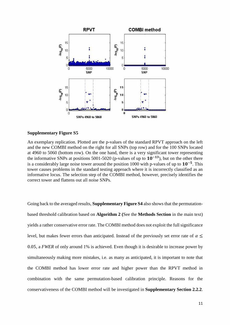
11


An exemplary replication. Plotted are the p-values of the standard RPVT approach on the left

and the new COMBI method on the right for all SNPs (top row) and for the 100 SNPs located

at 4960 to 5060 (bottom row). On the one hand, there is a very significant tower representing

the informative SNPs at positions 5001-5020 (p-values of up to 𝟏𝟎−𝟏𝟑), but on the other there

is a considerably large noise tower around the position 1000 with p-values of up to 𝟏𝟎−𝟓. This

tower causes problems in the standard testing approach where it is incorrectly classified as an

informative locus. The selection step of the COMBI method, however, precisely identifies the

correct tower and flattens out all noise SNPs.

Going back to the averaged results, Supplementary Figure S4 also shows that the permutation-

based threshold calibration based on Algorithm 2 (See the Methods Section in the main text)

yields a rather conservative error rate. The COMBI method does not exploit the full significance

level, but makes fewer errors than anticipated. Instead of the previously set error rate of 𝛼 ≤

0.05, a FWER of only around 1% is achieved. Even though it is desirable to increase power by

simultaneously making more mistakes, i.e. as many as anticipated, it is important to note that

the COMBI method has lower error rate and higher power than the RPVT method in

combination with the same permutation-based calibration principle. Reasons for the

conservativeness of the COMBI method will be investigated in Supplementary Section 2.2.2.

12

To understand the results in more detail, we now investigate the individual data sets.

Supplementary Figure S6 shows for all 10,000 synthetic data sets the level of difficulty of the

problem, represented by the power that can be achieved via RPVT, and how well it can be

solved using the COMBI method, represented by the gain in TPR of the COMBI method over

RPVT. In the majority of cases, the COMBI method helps performance, i.e., increases the TPR.

However, it decreases performance in very few cases (about 3% of the 10,000 data sets). As

expected, those cases represent difficult problems with high noise where the baseline TPR of

RPVT is very low.


The TPR gain of the COMBI method is plotted as a function of the TPR of RPVT, which is

interpreted as a measure of the difficulty of the problem (i.e. level of noise). Each dot represents

one replication and indicates how much can be gained in terms of TPR by applying the COMBI

method instead of RPVT for this specific data set. In most cases, the TPR gain is positive,

indicating an increase in performance when using the COMBI method. The few cases where

power is lost with the COMBI method are characterized by a high level of difficulty in the first

place, i.e. RPVT TPR is low. Four replications are highlighted. Three of them represent special

cases with extraordinary characteristics (i.e. maximum TPR gain, minimum TPR gain with low

and high noise) and the fourth represents an average run with medium TPR gain and medium

noise. See Supplementary Figure S7 for the individual results of those replications.

13

In order to investigate the different situations to be encountered in a real world setting, we now

analyze a number of special replications. Detailed plots of exemplary runs that either represent

an average run (i.e. medium TPR gain and medium noise) or have extraordinary characteristics

(i.e. maximum TPR gain, minimum TPR gain with low and high noise) are shown in

Supplementary Figure S7. The first row represents the replication with maximum TPR gain

where the COMBI method worked extremely well. Although there is a lot of noise and the

tower of SNPs associated with the phenotype located at positions 5001-5020 is not very high

in this example, the COMBI method finds it accurately. An average replication with medium

noise and medium TPR gain, i.e., where both methods find the tower and the COMBI method

can only moderately help performance, is presented in the second row. The third example

illustrates that RPVT is sufficient for very easy problems (i.e. low noise and high tower yielding

minimum TPR gain), and that using the COMBI method does not decrease performance. The

most crucial case is presented in the last row. In this worst case scenario of a minimum TPR

gain and high noise, there is an extremely small tower that is very hard to identify. In addition,

there is another high-noise tower with very high SVM weights. In contrast to the RPVT

approach, which identifies the correct tower, the COMBI method selects the wrong tower. This

example shows that the COMBI method selects the wrong towers in very few cases.

14


Detailed plots of exemplary runs with (1) maximum TPR gain, (2) medium TPR gain and

medium noise, (3) minimum TPR gain and low noise and (4) minimum TPR gain and high

noise. The p-values of the COMBI method and the SVM weights are shown for each replication

the p-values of RPVT. The first three replications represent problems where the COMBI

method does better or at least as well as the RPVT approach. The last example illustrates that

the COMBI method selects the wrong towers in some cases.

We now investigate whether these pathological cases can be identified a priori. As observed in

Supplementary Figure S7, these cases are characterized by a high noise level, indicating that

a very hard problem must be solved. Finding the data sets where an SVM trained for

classification of the subjects does not have high accuracy is an intuitive idea. Those cases would

be expected to be those where the COMBI method also fails, which is exactly what can be seen

when investigating the SVM accuracies for each replication in Supplementary Figure S8. The

problematic cases -- where power is lost with the COMBI method -- are indeed characterized

by a low SVM classification accuracy. These cases can thus roughly be estimated in advance,

and a measure of trust in the results of the COMBI method can be given for each replication.

15


For each replication, the AUC gain of the COMBI method is plotted against the corresponding

SVM accuracy. Negative AUC gain marks the problematic cases where power is lost. It can be

seen that the COMBI method only yields a loss in performance in some of the experiments with

low SVM accuracy, which means that problematic cases can be identified and a measure of

trust can be reported along with the results of the COMBI method for each data set.

2.2.2. Conservativeness of the FWER control

Supplementary Figure S4 showed that the COMBI method achieves an overall FWER of

around 1%, even though the resampling threshold was a priori set to guarantee that FWER≤

5%. We provide an explanation for the conservativeness of the COMBI method in the following

section.

An effect that makes the COMBI method conservative is the different number of uninformative

(or “noisy”) SNPs the threshold calibration is based on and eventually applied to. To illustrate

this, assume that k equals 30, indicating that the 30 SNPs with the highest SVM weights are

selected for each replication in the permutation test and p-values are computed for only those.

The significance threshold based on these p-values is then determined. As the threshold is

calibrated on random labels, it is based on the p-values of 30 uninformative SNPs. However,

when we train on real labels when applying the threshold, it is very likely that 20 informative

SNPs are selected as part of the 30 highest ranked SNPs. There are thus only 10 spots left for

the noisy SNPs, which are rejected only if they exceed the threshold. Having 10 instead of 30

16

noisy SNPs makes an erroneous rejection much more unlikely. Thus, the COMBI method

makes fewer mistakes than anticipated and is rather conservative. To validate this hypothesis,

we perform a number of experiments where parameter values are altered to achieve the correct

FWER of 5%. In the first experiment, k is increased in a way that the number of noisy SNPs

remains constant. Instead of only selecting k SNPs (noisy or informative), we select the

informative SNPs that are amongst the k best SVM weights; in addition to that, the best k noisy

SNPS, i.e., 𝑘𝑖∗ = 𝑘 + 𝑛𝑇𝑃,𝑖 where 𝑛𝑇𝑃,𝑖 is the number of true positives among the k best SNPs

in the i-th replication of the experiment. This should eliminate the effect described above and

hence yield a FWER closer to that set prior to the permutation test. Applying this slightly

modified COMBI method to the 10,000 semi-real data sets leads to a FWER of around 5% and

thus supports this hypothesis. Note that these modifications can only be applied to data sets

where the ground truth, and thus 𝑛𝑇𝑃,𝑖, is known. To investigate this effect in more detail, we

now perform an experiment where we increase the number of selected SNPs, in order to check

whether this also yields a less conservative error rate. Supplementary Figure S9 shows that

increasing k to a maximum of 1,000 yields a FWER of 5%. This is reasonable, as increasing k

means increasing the fraction of noisy SNPs in the set of SNPs that are picked via the

permutation-based calibration procedure. For k=1,000, all SNP towers are selected and we

simply perform the standard RPVT method which yields a non-conservative FWER of 5%. The

fewer the selected SNPs, the better the curve and the more conservative the permutation-based

calibration. The optimal curve but also most conservative threshold calibration is reached for k

= 30, which is the parameter chosen for all other applications of the COMBI method. For a

lower value of k, the FWER-TPR-curve is noticeably below the optimal one, and the

permutation-based calibration suffers a severe loss in power.

17


Results of the COMBI method for different values of k, the number of SNPs to select in the

screening step. (a) TPR is plotted against ENFR for increasing k from 10 to 500. The points

represent the results of the COMBI method after applying the permutation-based threshold. The

lime green curve of k = 30 is optimal. This is also the parameter value that yields the highest

power using the permutation-based calibration (lime green circle). The higher k, the less optimal

are the resulting curves (from green over blue to purple), but also the closer is the ENFR of the

permutation-based calibration method to the anticipated 5%. Decreasing k below 30 results in

a severe loss in power (red curve). (b) Mean and standard deviation of ENFR are shown for

different values of k. The maximum error rate which equals the pre-set bound of 𝜶 ≤ 𝟎. 𝟎𝟓 is

attained for k=1,000, which corresponds to selecting almost all towers and therefore is almost

equivalent to applying RPVT.

The next parameter to be investigated is the noise parameter, which is involved in the data

generation process. We expect that for high levels of noise, i.e. when there is basically a lack

of any kind of real association, the FWER of the COMBI method approaches the expected 5%

because the 30 selected SNPs selected are all noisy SNPs. Thus, the threshold is not only based

on noisy SNPs but also only applied to noisy SNPs. Observe from Supplementary Figure S10

that for 𝛼 = 0.05, the correct FWER is actually achieved for a maximum level of noise.

However, the curve is optimal for minimum noise where the identification of true associations

is much easier. This experiment supports the hypothesis presented earlier.

18


Results of the COMBI method for different values of the noise parameters 𝛄 where the low

values correspond to high noise and the high values to low noise in the process of simulating

the datasets. (a) TPR is plotted against ENFR for increasing the noise parameter from 0.25 to

1000. The points represent the results of the COMBI method after applying the permutation test

threshold. The curve is optimal for minimum noise (purple curve), which was to be expected

as a low level of noise makes true associations easier to detect. (b) Mean and standard deviation

of ENFR are shown for different values of the noise parameters. The maximum error rate, which

equals the pre-set bound of 𝜶 ≤ 𝟎. 𝟎𝟓, is attained for a noise parameter of 0.25, which is almost

equivalent to having maximum noise and therefore no informative SNPs associated with the

disease.

Observe from Supplementary Figure S11 that we achieve the error rate for filter length 1 that

we would expect after setting it to 𝛼 ≤ 0.05 in the permutation test. The error rate decreases

and power increases with increasing filter length up to 35. The method yields higher error rates

and less power for greater filter lengths. We therefore decided to use a filter length of 35, which

yields optimal but conservative results. We learn from these experiments that the proposed

method may achieve lower error rates and higher TPR than anticipated.

19


Results of the COMBI method for different values of the filter window size l. (a) TPR is plotted

against ENFR for increasing l from 1 to 501, where the former corresponds to applying no filter

at all and the latter to an extremely flattening filter. The points represent the results of the

COMBI method after applying the permutation-based threshold. The curve is optimal for a filter

window size of 35. This finding is in agreement with what Alexander and Lange4 found. (b)

Mean and standard deviation of ENFR are shown for different values of the filter window size

l. The maximum error rate is attained for filter length 1, which corresponds to applying no filter.

2.2.3. Further experiments

Choosing an optimal SVM parameter using cross-validation-based model selection in each

repetition of the Westfall-Young permutation procedure did not result in a higher power of the

COMBI method. Performance results for constant and cross-validated C were hardly

distinguishable. Thus, time-consuming cross-validation was avoided for C, and a fixed C was

used for all further applications of the COMBI method.

20

2.2.4. Comparison to other state of the art methods

In addition to comparing the COMBI method with the RPVT approach, we investigate here

whether slight alterations and simplifications of the COMBI method can achieve the same level

of effectiveness and also examine other appropriate state-of-the-art algorithms using semi-real

data (See Supplementary Section 2. for a description of these semi-real data experiments and

the Discussion Section of the main paper for a discussion of related machine learning work).

Beginning with the investigation of simplifications of the COMBI method, we now present the

results of corresponding simulations. As mentioned earlier, applying a moving average filter to

the SVM weights prior to the selection step is crucial. Observe in Supplementary Figure S12

that the COMBI method cannot increase power or precision of RPVT at all without this filtering

step.

To find out whether the filtering step, which improves the performance of the COMBI method,

can also be applied to the p-values, 𝑝𝑗, in log-space in order to achieve the same effect, we

define 𝑤𝑗 ≔ − log10 𝑝𝑗 and apply the filter as described in Summary of the COMBI method

and Figure 1 (see main text). We employ RPVT in the original p-value space. Supplementary

Figure S12 illustrates that this decreases the performance of the RPVT method and thus cannot

reach the effectiveness of the COMBI method. In conclusion, the COMBI method is most

effective when both screening approaches, i.e. SVM and filter screening, are applied

simultaneously (Supplementary Figure S4).

Besides checking whether easy simplifications of the COMBI method achieve the same effect,

the performances of other competitor methods were investigated. As discussed in the

Discussion Section of the main paper, there are a number of related machine learning methods,

out of which we selected three as representatives to be compared to the COMBI method in this

simulation setup.

21

The most related method separates the two steps of COMBI method, i.e. machine learning and

statistical testing, from each other and was proposed by Wasserman and Roeder11. In the course

of this algorithm, half of the data points (i.e. half of the individuals) are first randomly selected

and an SVM is trained to identify the k SNPs with the highest corresponding weights. In the

second step, p-values are computed on the other half of the data points considering only the

SNPs identified in the previous step. Even though the significance threshold 𝛼 can now simply

be corrected with 𝛼𝑛𝑒𝑤 = 𝛼/𝑘 (which is much less conservative than the Bonferroni correction

𝛼𝐵𝑜𝑛𝑓. = 𝛼/𝑑 when considering all SNPs), this method comes with a loss of power (see

Supplementary Figure S13), where the corresponding curves are constantly below the curve

of the regular COMBI method.

Meinshausen et al.10 present an extension of the method proposed by Wasserman and Roeder11.

Instead of splitting the data once into two sets and using one for SVM training and the other for

statistical testing, they suggest aggregating the results of multiple random splits, arguing that

this will decrease error rates and increase power. They propose using quantiles as summary

statistics for the p-values of the multiple splits. After defining qγ (・) to be the empirical γ-

quantile function the p-value for each predictor j = 1, …, p is calculated with Pj = min {1, (1

−log γmin) infγ ∈(γmin,1)

Qj(γ ) }where Qj(γ ) = min{1, qγ({P(b)j /γ ; b = 1, . . . ,B})}. In our

simulation, this method does not reach the performance level of the COMBI method (See

Supplementary Figure S13) and also fails to reach that of the RPVT approach. The results

indicate that it may be more effective to use the full data set for selection of candidate SNPs

and multiple testing on these SNPs (as done in the course of the COMBI method), rather than

using a subset for selection and another subset for testing (as done in the single- and multi-split

methods by Wasserman and Roeder11 and Meinshausen et al.10).

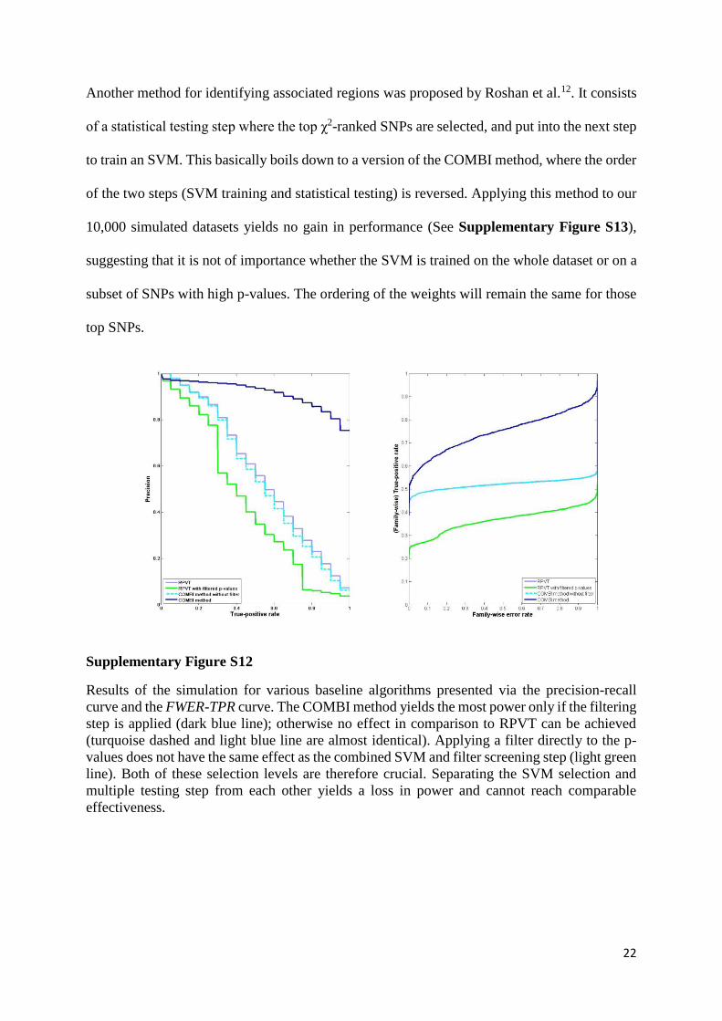
22

Another method for identifying associated regions was proposed by Roshan et al.12. It consists

of a statistical testing step where the top χ2-ranked SNPs are selected, and put into the next step

to train an SVM. This basically boils down to a version of the COMBI method, where the order

of the two steps (SVM training and statistical testing) is reversed. Applying this method to our

10,000 simulated datasets yields no gain in performance (See Supplementary Figure S13),

suggesting that it is not of importance whether the SVM is trained on the whole dataset or on a

subset of SNPs with high p-values. The ordering of the weights will remain the same for those

top SNPs.


Results of the simulation for various baseline algorithms presented via the precision-recall

curve and the FWER-TPR curve. The COMBI method yields the most power only if the filtering

step is applied (dark blue line); otherwise no effect in comparison to RPVT can be achieved

(turquoise dashed and light blue line are almost identical). Applying a filter directly to the p-

values does not have the same effect as the combined SVM and filter screening step (light green

line). Both of these selection levels are therefore crucial. Separating the SVM selection and

multiple testing step from each other yields a loss in power and cannot reach comparable

effectiveness.

23


Results of the simulation for various competitor algorithms presented via the precision-recall

curve and the FWER-TPR curve. The COMBI method yields the highest power, while no other

method can achieve the same performance. Note that the yellow curve is almost identical to the

green one in the figure to the right, which is why it is hardly visible.

24

3. Analysis of real data (WTCCC, 2007)

3.1. Data preparation

Genotype and phenotype data for the seven disease and two control groups used in the WTCCC1

were downloaded from the EGA website (European Genome-phenome Archive, ega.crg.eu)

after being granted the corresponding access. Seven case-control datasets, one for each disease,

were built combining both control groups. SNPs and samples that did not fulfill the quality

control in the original WTCCC paper were removed from each dataset using the lists provided

at the WTCCC site.

Based on lists provided by the WTCCC (see www.wtccc.org.uk), we removed an additional set

of 579 false-positive SNPs from analysis (for instance, SNPs that are significant, isolated hits,

with no significance in surrounding SNPs in high LD, i.e., with no “tower” around them). Since

these lists seemed to lack the information corresponding to the coronary artery disease (CAD)

study, all genome-wide significant SNPs (<5e-7) for that study that did not appear in the original

WTCCC paper were manually removed.

3.2. Automatic validation procedure

Our automatic validation procedure is based on identifying associations to a disease reported in

the GWAS catalog for either the target SNP or other SNPs in high LD with them. That is, to

validate the SNPs COMBI identifies as good predictors upon analysis of the WTCCC data, we

used the conservative criterion of ascertaining whether our candidate SNPs or other SNPs in

high LD with them had been reported as associated to the corresponding disease by independent

GWAS published after the WTCCC study. Our validation procedure considers a physical

window of 200kb around any given SNP associated with a given disease and selects all SNPs

within this window presenting strong LD with the target SNP. LD calculations were performed

with PLINK13 and were based on the genomic sequences of the 85 CEU individuals from Phase

1 of the 1000 Genomes Project. Runs with different thresholds were performed: (r2>0.7, >0.8,

25

>0.9 and =1) without any change in our results. For the resulting high-LD SNPs, our algorithm

queries the GWAS catalog to check if these SNPs have been associated to a disease with p-

values <10-5. A hit indicates that a GWAS other than the original WTCCC study reported this

SNP to be associated with the relevant disease and, thus, that independent evidence validates

the discovery.

3.3. Prediction performance

In Supplementary Table S1, we present the prediction performances of an SVM as used in the

first step of the COMBI method applied to the WTCCC data in comparison to the reported

performance rates of other machine learning methods presented in the Discussion Section of

the main paper. We use the area under the receiver operating characteristic curve (AUC) as the

measure of performance.

Supplementary Table S1

Reported Prediction Performances (AUC in %) of the SVM in the first step of the COMBI

method and other machine learning methods.

SVM (first step of

COMBI method)

Mittag

et al.14

Davies

et al.15

Evans

et al.16

Kooperberg

et al.17

Wei et

al.18

BD 70.4 61 - 66.8 - -

CAD 62 - 60.2 60.0 - -

CD 64.9 - - 61.0 63.7 -

HT 65.8 - - 62.7 - -

RA 63 - - 66.6 - -

T1D 74.9 88 - 74.9 88 89

T2D 63.4 62 - 60.1 - -

Note that the AUC values of the optimal parameter values and methodological settings are

reported for all methods (i.e. we chose the most successful feature encoding, p-value feature

26

selection, statistical test, SVM solver etc., for the SVM of the COMBI method, and the optimal

parameter values corresponding to the methodology applied in that paper for all other methods).

The linear SVM of the COMBI method performs similarly well as most other competing

methods, except for type 1 diabetes, where a non-linear kernel performs better. We excluded

the results of Quevedo et al.19 from this table, since they were flawed by a lack of a step in their

data processing procedure (J.R. Quevedo, personal communication).

3.4. Stability analysis

Stability is a desirable property of any SNP-selection method: if a method is not stable, it could

either indicate that too many locations are selected, meaning that the result contains a random

subset of non-significant SNPs, or that not enough locations are selected, so that the result

contains only a random subset of the significant SNPs.

To investigate stability, we proceeded as follows: the original data was randomly split into two

equally sized subsets (of individuals), A and B, for a number of 10 repetitions. The method

under scrutiny, i.e., either the COMBI method or standard RPVT, is applied separately to the

data from sets A and B, leading to sets S(A) and S(B) of respectively reported SNPs. Using the

Tanimoto Index20 𝑇(𝑆(𝐴), 𝑆(𝐵)) =|𝑆(𝐴)∩𝑆(𝐵)|

|𝑆(𝐴)∪𝑆(𝐵)|, the similarity of these two sets and thus the

stability of the used method were measured. Here |𝑆| denotes the cardinality of the set S. In this

manner, the stability of the COMBI method can be compared to the stability of standard RPVT.

Simulation results considering internal stability of the two methods when applied to the

WTCCC Crohn’s Disease data are shown in Supplementary Figure S14. COMBI produces

more stable results than RPVT. The Tanimoto stability index is plotted against the mean number

of reported associations, i.e. |𝑆(𝐴)|+|𝑆(𝐵)|

2. When we repeatedly split the data into two parts and

investigate how similar the results of the two methods are in the two subsets, we find that the

27

results of the COMBI method are more similar and thus more stable. This is true for all levels

of ENFR and thus for the mean number of reported associations.


Tanimoto Stability Indices for Crohn’s Disease. We observe that the stability of the COMBI

method is higher than that of RPVT. Note that higher Tanimoto index denotes higher stability.

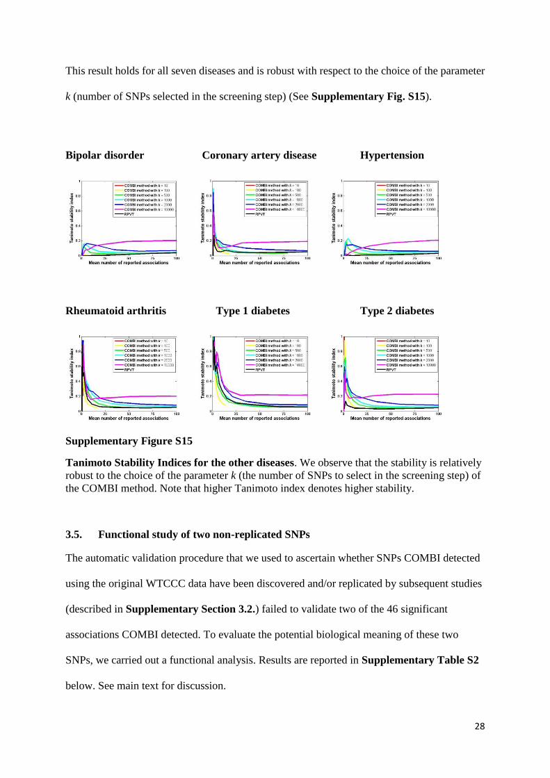
28

This result holds for all seven diseases and is robust with respect to the choice of the parameter

k (number of SNPs selected in the screening step) (See Supplementary Fig. S15).

Bipolar disorder Coronary artery disease Hypertension

Rheumatoid arthritis Type 1 diabetes Type 2 diabetes


Tanimoto Stability Indices for the other diseases. We observe that the stability is relatively

robust to the choice of the parameter k (the number of SNPs to select in the screening step) of

the COMBI method. Note that higher Tanimoto index denotes higher stability.

3.5. Functional study of two non-replicated SNPs

The automatic validation procedure that we used to ascertain whether SNPs COMBI detected

using the original WTCCC data have been discovered and/or replicated by subsequent studies

(described in Supplementary Section 3.2.) failed to validate two of the 46 significant

associations COMBI detected. To evaluate the potential biological meaning of these two

SNPs, we carried out a functional analysis. Results are reported in Supplementary Table S2

below. See main text for discussion.

29


Functional analysis of two SNPs detected by COMBI and not replicated in subsequent GWAS

studies.

SNP detected by COMBI

rs11110912 rs6950410

Disease HT (Hypertension) T1D (Type 1 diabetes)

Chr / Position

(hg19) 12:102042213 7:4038917

Functional

consequence

Intronic MYBPC1 (myosin binding

protein C)

Intronic SDK1 (sidekick cell adhesion

molecule 1)

OMIM1 Yes (involved in familial hypertrophic

cardiomyopathy) -

GWAS Catalog2 No No

Genes (in 200 Kb

window) MYBPC1, CHPT1, SYCP3 SDK1

eQTL activity3 (P-

value) CHPT1 (P<10-8) -

RegulomeDB4 1d ("strong") -

Haploreg5 Transcription factor activity (BATF,PU1) DNAse activity (in Osteoblasts) 1 OMIM. Role in disease evidence of the gene the associated SNP lies in (available at http://omim.org/) 2 GWAS Catalog. Presence in the "reported gene" field in the GWAS Catalog (http://www.genome.gov/gwastudies/) 3 eQTL activity. Evidence about the activity as eQTL in blood of the associated SNP (gathered from the "Blood eQTL browser";

http://genenetwork.nl/bloodeqtlbrowser/) 4 RegulomeDB. Summary of DNA regulatory evidence (in http://regulomedb.org/) 5 Haploreg. Noncoding regulatory evidence of the haplotype block (www.broadinstitute.org/mammals/haploreg/haploreg.php)

3.6. Comparison to Fast-LMM models

We compared COMBI against another state-of-the-art method by Lippert et al.21 who devised

a novel univariate analysis method to improve WTCCC findings and implemented a linear

mixed model (LMM) to uncover new epistatic associations by means of brute force comparison

of pairwise interactions. They applied both methods to the seven WTCCC diseases, searching

for new univariate signals and for epistatic associations.

For the univariate analysis, they reported a total of 573 novel SNP-disease associations21 with

p-values less than 5x10-7), covering all WTCCC diseases but CAD, for which no novelty was

reported. Most novel SNPs were mapped in the same loci, so we selected representative markers

for each locus through the LD pruning option in PLINK. We computed pairwise LD with a

sliding window of two SNPs (with steps of 1 SNP at a time). We discarded one SNP out each

pair if they were in high LD (R² ≥ 0.8). The final SNP lists, consisting in 1 for BD, 0 for CAD,

19 for CD, 1 for HT, 3 for RA, 39 for T1D and 9 for T2D, was run through our validation

30

pipeline using the same parameters that we use for COMBI in the present work (physical

distance to tag-SNP: < 200 kb. Linkage disequilibrium with tag-SNP: R² ≥ 0.8). The number of

“true positive” hits (that is, of discoveries that have been validated in the literature) was limited,

with only five of them featured in GWAS published after the WTCCC hits (CD: 3 hits, RA: 1

and T2D 1 hit each). This figure is much smaller than for COMBI (See Supplementary Table

S3).

Supplementary Table S3 Not only does COMBI give rise to more validated discoveries, but these

discoveries cover the whole range of WTCCC diseases.


Comparison of COMBI against LMM univariate method. Only the three diseases indicated in

table were considered, as these were the only ones which reported hits by LMM validated in

further independent studies.

DISEASE COMBI set

of SNPs

COMBI

hits

LMM univariate

set of SNPs

LMM

univariate

hits

Binomial p-

value

Crohn's

Disease 11 8 19 3 4.07x10-5

Rheumatoid

Arthritis 3 1 3 1 NS

Type 2

Diabetes 8 3 9 1 0.049

The epistasis analyses by Lippert et al.,21 consisted of brute force computing of all possible

pairwise SNP associations for 6 diseases (~63 billion pairs; no hits reported for Crohn´s

disease), and testing their epistatic interaction in disease risk. The authors reported a final list

consisting in 707 pairs of SNPs with p-values lower than 7.9 x 10-13 for each phenotype

analyzed in WTCCC data. All individual SNPs taking part in the reported significant

interactions were checked against our validation pipeline. We are aware that this is only a partial

validation, since epistasis is not the simple addition of separated SNP effects, which are those

that are registered in the GWAS catalog, but some associations still could emerge.

31

Applying the same LD pruning method than for the univariate method, we ended up with the

following number of SNPs per each disease: 2 for BD, 32 for CAD, 0 for CD, 2 for HT, 7 for

RA, 13 for T1D and 2 for T2D. By running these markers through our validation pipeline, we

found a single association for T1D, while for the other diseases no markers were found. A

comparison against COMBI hits for type 1 diabetes can be seen in Supplementary Table S4.


Comparison of COMBI against LMM epistatic method. Only T1D was subject to comparison.

DISEASE COMBI set of

SNPs

COMBI

hits

LMM epistatic set

of SNPs

LMM epistatic

hits

Binomial p-

value

Type 1

Diabetes 9 6 9 1 1.1x10-4

32

3.7. Runtime analysis and implementation details

The COMBI method is implemented in R, Matlab/Octave and Java as a part of the GWASpi

toolbox 2.0 (https://bitbucket.org/gwas_combi/gwaspi/, login user name:

gwas_combi_guest, password: combi123.). The complete method is available in all languages

and there are no substantial differences in implementation. See Supplementary Table S5 for

implementation details

Supplementary Table S5: Specialities and details about used packages for all

implementations of the COMBI method.

The runtime of the method depends on a variety of factors such as available cluster memory,

hardware resources and operating system. For this analysis we have run the method with the

implementation on the following technical platform: 40 * Intel(R) Xeon(R) CPU E5-2650 v3

@ 2.30GHz 64bit, 128GB RAM, Ubuntu 14.04.4 LTS (GNU/Linux 3.13.0-79-generic x86_64).

The analysis of WTCCC’s data on Crohn’s disease chromosome 18 (assuming calculations on

more chromosomes can be computed in parallel if necessary) took 9h 15min 24s using the

Matlab/Ovtave implemenation. See Supplementary Table S6 for information on how the

computation time spread across the various steps of the COMBI method and how it varied for

the different implementations in Java, Matlab/Octave and R.

Language Speciality Used packages

Java COMBI method fully implemented

supports other algorithms within the

GWASpi software

desktop computer oriented

libLinear22, libSVM23, apache

commons math24

Matlab/Octave COMBI method fully implemented

cluster oriented

libLinear22

R COMBI method fully implemented LiblineaR25, qqman26,

data.table27, gtools28, snpStats29

33

Supplementary Table S6: Runtime analysis of the COMBI method. The complete method

was applied to WTCCC data from chromosome 18 investigating Crohn’s Disease. 1000

replications were run in both permutation procedures. Please note, that the permutation

procedures are still being improved for both Java and R implementations and running times

are provisional.

Matlab/Octave

(Here GNU

Octave version

3.8.1)

Java

(Here SUN JDK

version 1.8.0_77

64bit, Maven

version 3.3.9)

R

(Here R version

3.0.2 (2013-09-

25), Frisbee

Sailing)

Training of SVM (first

step of COMBI)

21s 8min 30s 41min 55s

Calculation of raw p-

values (second step of

COMBI)

3s 25s 1min 46s

Permutation procedures

for the calculation of

significance thresholds

9h15min 8d 3h 30min >1month

Overall 9h15min24s 8d 3h 38min 55s >1month

We should point out that with respect to running time, COMBI cannot compete with

traditional GWAS methods like raw p-value thresholding. However, as we stress in the paper,

we believe that the contribution of the present work lies in providing a new method that

considerably improves power and precision rather than in improving running time.

34

References of supplementary material

1. Wellcome, T., Case, T. & Consortium, C. Genome-wide association study of 14,000

cases of seven common diseases and 3,000 shared controls. Nature 447, 661–78

(2007).

2. Westfall, P. & Young, S. Examples and Methods for p-Value Adjustment. (Wiley,

1993).

3. Fan, J. & Lv, J. Sure independence screening for ultrahigh dimensional feature space.

J. R. Stat. Soc. Ser. B Statistical Methodol. 70, 849–911 (2008).

4. Alexander, D. H. & Lange, K. Stability selection for genome-wide association. Genet.

Epidemiol. 35, 722–728 (2011).

5. Salanti, G. et al. Underlying genetic models of inheritance in established Type 2

diabetes Associations. American Journal of Epidemiology 170(5), 537-545 (2009).

6. Clarke , G. M., Anderson, C. A., Pettersson, F. H., Cardon, L. R., Morris, A. P., &

Zondervan, K. T. Basic Statistical analysis in genetic case-control studies. Nature

Protocols 6(2), 121–133 (2011).

7. Marigorta, U.M. & Navarro, A. High Trans-ethnic Replicability of GWAS Results

Implies Common Causal Variants. Plos Genetics, 9(6), e1003566 (2013).

8. Marigorta, U.M., Rodriguez, J.A. & Navarro, A. "GWAS: a milestone in the road from

genotypes to phenotypes" in Appasani, K. (ed.). Genome-Wide Association Studies:

From Polymorphism to Personalized Medicine. Cambridge University Press, pp. 12–

25. (2016).

9. Gibson, G. Rare and common variants: twenty arguments. Nature Review Genetics

13, 135-145 (2012).

10. Meinshausen, N., Meier, L. & Bühlmann, P. p-Values for High-Dimensional

Regression. J. Am. Stat. Assoc. 104, 1671 (2009).

11. Wasserman, L. & Roeder, K. High-dimensional variable selection. Ann. Stat. 2178–

2201. doi:10.1214/08-AOS646 (2009).

12. Roshan, U., Chikkagoudar, S., Wei, Z., Wang, K. & Hakonarson, H. Ranking causal

variants and associated regions in genome-wide association studies by the support

vector machine and random forest. Nucleic Acids Res. 39 , e62–e62 (2011).

13. Purcell, S. et al. PLINK: a tool set for whole-genome association and population-based

linkage analyses. Am j Hum. Genet 81, 559–575 (2007).

35

14. Mittag, F. et al. Use of support vector machines for disease risk prediction in genome-

wide association studies: Concerns and opportunities. Hum. Mutat. 33, 1708–1718

(2012).

15. Davies, R. W. et al. Improved Prediction of Cardiovascular Disease Based on a Panel

of Single Nucleotide Polymorphisms Identified Through Genome-Wide Association

Studies. Circ. Cardiovasc. Genet. 3 , 468–474 (2010).

16. Evans, D. M., Visscher, P. M. & Wray, N. R. Harnessing the information contained

within genome-wide association studies to improve individual prediction of complex

disease risk. Hum. Mol. Genet. 18, 3525–31 (2009).

17. Kooperberg, C., LeBlanc, M. & Obenchain, V. Risk prediction using genome-wide

association studies. Genet. Epidemiol. 34, 643–52 (2010).

18. Wei, Z. et al. From Disease Association to Risk Assessment: An Optimistic View from

Genome-Wide Association Studies on Type 1 Diabetes. PLoS Genet 5, e1000678

(2009).

19. Quevedo, J. R., Bahamonde, A., Perez-Enciso, M. & Luaces, O. Disease Liability

Prediction from Large Scale Genotyping Data Using Classifiers with a Reject Option.

IEEE/ACM Trans. Comput. Biol. Bioinforma. 9, 88–97 (2012).

20. Rogers, D. J. & Tanimoto, T. T. A Computer Program for Classifying Plants. Sci. 132,

1115–1118 (1960)

21. Lippert, C., Listgarten, J., Davidson, R.I., Baxter, J., Poon, H., Kadi, C.M. &

Heckerman, D. An exhaustive epistatic SNP association analysis on expanded

Wellcome Trust data. Sci. Rep. 3, 1099 (2013).

22. Fan, R.-E., Chang, K.-W., Hsieh, C.-J., Wang, X.-R. & Lin, C.-J. LIBLINEAR: A

Library for Large Linear Classification. Journal of Machine Learning Research 9,

1871-1874. Software available at http://www.csie.ntu.edu.tw/~cjlin/liblinear (2008).

23. Chang, C.-C. & Lin, C.-L. LIBSVM: a library for support vector machines. ACM

Transactions on Intelligent Systems and Technology 2(27), 1-27. Software available at

http://www.csie.ntu.edu.tw/~cjlin/libsvm (2011).

24. The Apache Software Foundation. Commons Math: The Apache Commons

Mathematics Library. Java version 1.7. Software available at

http://commons.apache.org/proper/commons-math/ (2016).

25. Helleputte, T. & Gramme, P. LiblineaR: Linear Predictive Models Based on the

LIBLINEAR C/C++ Library. R package version 1.94-2 from

http://dnalytics.com/liblinear/ (2015).

26. Turner, S.D. qqman: an R package for visualizing GWAS results using Q-Q and

manhattan plots. biorXiv DOI: 10.1101/005165. R package version 0.1.2 from

http://cran.r-project.org/web/packages/qqman/ (2014).

36

27. Dowle, M., Srinivasan, A., Short, T. & Lianoglou, S. with contributions from Saporta,

R. & Antonyan, E. data.table: Extension of Data.frame. R package version 1.9.6. from

https://CRAN.R-project.org/package=data.table (2015).

28. Warnes, G.R., Bolker, B. & Lumley, T. gtools: Various R Programming Tools. R

package version 3.5.0. from https://CRAN.R-project.org/package=gtools (2015).

29. Clayton, D. snpStats: SnpMatrix and XSnpMatrix classes and methods. R package

version 1.22.0 from http://bioconductor.org/packages/release/bioc/html/snpStats.html

(2015).

Documents

Combining Multiple Hypothesis Testing with …1fd18a91-bc61-4bf3-b798-cd38a91c5399/Mi… · Combining Multiple Hypothesis Testing with Machine Learning Increases the Statistical Power