Embed Size (px)
Citation preview
Combustion InstabilityScreech in Gas Turbine Afterburners
A ThesisSubmitted for the Degree of
Doctor of Philosophyin the Faculty of Engineering
by
Kampa Ashirvadam
Department of Aerospace EngineeringIndian Institute of Science
Bangalore - 560012
July 2007
Acknowledgements
I am grateful to Shri T. Mohana Rao, Director GTRE, Bangalore, who kindlypermitted me to carryout the research on screech phenomenon by using the af-terburner test facility and computing facilities that are available at GTRE. I amalso grateful to former Directors Dr. K. Ramachandra, Shri V. Sundararajan andShri S. C. Kaushal, who encouraged me to pursue this work.
I am grateful to Prof. P. J Paul, Department of Aerospace, Indian Instituteof Science, who introduced me to the subject of Combustion Instability andmathematical modelling, which immensely helped me to carry out the researchwork. He also supervised the entire program, by providing excellent guidancein theoretical analysis and in the conduction of experiments. I acknowledge thefull support of Dr.A P Haran, Group Director of Afterburner Division, GTREwho spared me for this work and provided with excellent technical expertise toincorporate in the analysis. I thank Dr.S Kishore Kumar for supervising thetheoretical analysis and offering suggestions in organising the thesis content.
I specially thank Prof. B.N.Raghunandhan, Chairman, Department of Aero-space Engineering, Indian Institute of Science for permitting me to carryout thework and submit beyond the permissible limit of Institute time. I am ever gratefulto Prof.M.L.Munjal, Department of Mechanical Engineering, Indian Institute ofScience, for leading me into the subject of acoustics, sparing his valuable time todiscuss the problem at various levels throughout this work.
I acknowledge the technical review carried out by Dr. J. J. Isaac, ActingDirector of NAL and Dr. K. V. L. Rao, Technical Advisor, ADA and offeringseveral suggestions in the area of analysis and testing. I am grateful to Smt.Meera Kaushal, GTRE who encouraged me at various levels to pursue this work.I express my sincere thanks to Dr.Venkataramanshankar, Additional Director,GTRE. I am indebted to Shri.T.Venkatakrishnaiah, Additional Director and Ms.S. Jayanthi, Divisional Head, Technical co-ordination division along with admin-istrative department of GTRE for dealing with DRDO head quarters for obtainingstudy leave and maintaining the correspondence.
I am grateful to Shri K. Venkataraju, Additional Director, (Instrumentation)GTRE for providing instrumentation along with necessary cabling for conduct-ing experiments. I thank Shri A. C. Bhaskar, and his team who provided thecompressed air whenever tests were conducted. I acknowledge the technical helpprovided by Shri.Sanjay Barad, Giridhar, Dilip and his team to acquire the datafrom the tests. Though there was unfavourable environment during testing dueto huge sound levels, his team cheerfully supported the work whenever tests need
i

ii
to be conducted and immediately allowed me to conduct the analysis.A partial list of my colleagues, who have helped me in many ways and created
a cheerful environment, includes, T. K. Murthy, N. R. Viswanathan, Davis, andmany more.I shall always cherish the time I spent with them.
The prayerful support of Rev.Lenin Kumar is gratefully acknowledged.With deep sense of gratitude I acknowledge my dear wife Satya, who with-
stood all the hard work by undertaking every small detail at home, including myhousehold responsibilities tirelessly. I am ever grateful to my sons, Jonathan andJabez who were deprived of many privileges and outings for several months.
Contents
Published Papers v
Abstract vi
List of Figures viii
List of Tables xi
Nomenclature xii
1 Introduction 11.1 Screech in afterburners . . . . . . . . . . . . . . . . . . . . . . . . . 11.2 Objectives of the Thesis . . . . . . . . . . . . . . . . . . . . . . . . 11.3 Description and operation of the afterburner . . . . . . . . . . . . 31.4 Organization of the thesis . . . . . . . . . . . . . . . . . . . . . . . 4
2 Literature Survey 52.1 Characteristics of oscillatory instabilities . . . . . . . . . . . . . . . 52.2 Combustion instabilities in afterburners . . . . . . . . . . . . . . . 72.3 Problem definition — Scope of analysis and testing . . . . . . . . . 13
3 Theory 163.1 The Governing Equations . . . . . . . . . . . . . . . . . . . . . . . 16
3.1.1 Boundary conditions . . . . . . . . . . . . . . . . . . . . . . 193.1.2 Method of solution . . . . . . . . . . . . . . . . . . . . . . . 20
3.2 SYSNOISE Software . . . . . . . . . . . . . . . . . . . . . . . . . . 223.3 Acoustic impedance of perforate liner geometry . . . . . . . . . . . 233.4 Nozzle admittance — for choked convergent nozzle . . . . . . . . . 253.5 Concluding Remarks . . . . . . . . . . . . . . . . . . . . . . . . . . 27
4 Combustion Source Response Function 284.1 Introduction . . . . . . . . . . . . . . . . . . . . . . . . . . . . . . . 284.2 Governing Equations . . . . . . . . . . . . . . . . . . . . . . . . . . 304.3 Flame Description . . . . . . . . . . . . . . . . . . . . . . . . . . . 30
4.3.1 The reaction rate . . . . . . . . . . . . . . . . . . . . . . . . 334.3.2 Steady state solution . . . . . . . . . . . . . . . . . . . . . . 33
4.4 Unsteady Response . . . . . . . . . . . . . . . . . . . . . . . . . . . 36
iii
Contents iv
4.5 Solution Procedure and software implementation . . . . . . . . . . 39
5 Experiments 425.1 Afterburner test facility . . . . . . . . . . . . . . . . . . . . . . . . 425.2 Afterburner test section . . . . . . . . . . . . . . . . . . . . . . . . 465.3 Afterburner test facility operation . . . . . . . . . . . . . . . . . . 51
6 Results and Discussion 526.1 Frequency characterization of test section . . . . . . . . . . . . . . 526.2 Identification of pure and coupled screech modes by analysis . . . . 586.3 Study of effectiveness of screech liner by variation in porosity . . . 606.4 Attenuation characteristics with 2.5 % porosity liner . . . . . . . . 636.5 Comparison of theoretical and experimental results . . . . . . . . . 71
7 Conclusions 77
A Nozzle Admittance 80A.1 Nozzle admittance for choked convergent nozzle . . . . . . . . . . . 80
Published Papers
1. Ashirvadam, K., Kishore Kumar, S., Haran, A. P. and Paul, P .J. Com-bustion Instabilities in Gas Turbine Afterburners. Fifteenth InternationalSymposium on Airbreathing Engines. September 2001, Bangalore
2. Ashirvadam, K., Kishore Kumar, S., Haran, A. P. and Paul, P. J. SoundPropagation in Afterburner Duct of a Gas Turbine Engine, Sixth NationalConference on Air Breathing Engines and Aerospace Propulsion. January2003, Bangalore.
3. Ashirvadam, K., Kishore Kumar, S., Haran, A. P. and Paul,P.J. Screech inGas Turbine Afterburner — a Combustion Instability Problem (Theory &Experiment). Sixteenth International Symposium on Airbreathing Engines.September 2004, Cleveland, US
v
Abstract
Gas turbine reheat thrust augmenters known as afterburners are used to provideadditional thrust during emergencies, take off, combat, and in supersonic flight ofhigh-performance aircrafts. During the course of reheat development, the mostpersistent trouble has been the onset of high frequency combustion instability,also known as screech, invariably followed by rapid mechanical failure. The cou-pling of acoustic pressure upstream of the flame stabilizer with in-phase heat-release downstream, results in combustion instability by which the amplitudeat various resonant modes — longitudinal (buzz — low frequency), tangentialor radial (screech — high frequency) – amplifies leading to deterioration of theafterburner components.
Various researchers in early 1950s have performed extensive testing on straightjet afterburners, to identify screech frequencies. Theoretical and experimentalwork at test rig level has been reported in the case of buzz to validate the heatrelease combustion models. In this work, focus is given to study the high fre-quency tangential combustion instability by vibro-acoustic software and the testsare conducted on the scaled bypass flow afterburner for confirmation of predictedscreech frequencies.
The wave equation for the afterburner is solved taking the appropriate geom-etry of the afterburner and taking into account the factors affecting the stability.Nozzle of the afterburner is taken into account by using the nozzle admittancecondition derived for a choked nozzle. Screech liner admittance boundary condi-tion is imposed and the effect on acoustic attenuation is studied. A new combus-tion model has been proposed for obtaining the heat release rate response functionto acoustic oscillations. Acoustic wave – flame interactions involve unsteady ki-netic, fluid mechanic and acoustic processes over a large range of time scales.Three types of flow disturbances exist such as : vortical, entropy, and acoustic.In a homogeneous, uniform flow, these three disturbance modes propagate in-dependently in the linear approximation. Unsteady heat release also generatesentropy and vorticity disturbances. Since flow is not accelerated in the regionof uniform area duct, vortical and entropy disturbances are treated as insignifi-cant, as these disturbances are convected out into atmosphere like an open-endedtube, but these are considered in deriving the nozzle admittance condition. Heatrelease fluctuations that arise due to fluctuating pressure and temperature aretaken into consideration. The aim is to provide results on how flames respondto pressure disturbances of different amplitudes and characterised by differentlength scales. The development of the theory is based on large activation energy
vi
Abstract vii
asymptotics. One-dimensional conservation equations are used for obtaining theresponse function for the heat release rate assuming the laminar flamelet modelto be valid. The estimates are compared with the published data and deviationsare discussed.
The normalized acoustic pressure variation in the afterburner is predicted us-ing the models discussed earlier to provide an indication of the resonant modesof the pressure oscillations and the amplification and attenuation of oscillationscaused by the various processes. Similar frequency spectrum is also obtainedexperimentally using a test rig for a range of inlet mean pressures and tempera-tures with combustion and core and bypass flows simulated, for confirmation ofpredicted results.
Without the heat source only longitudinal acoustic modes are found to beexcited in the afterburner test section. With heat release, three additional tan-gential modes are excited. By the use of eight probes in the circumferential crosssection of afterburner it was possible to identify the tangential modes by theirrespective phase shift in the experiments.
Comparison of normalized acoustic pressure and phase with and without theincorporation of perforate liner is made to study the effectiveness of the screechliner in attenuating the amplitude of screech modes. By the analysis, conclusion isdrawn about modes that get effectively attenuated with the presence of perforateliner. Parametric study of screech liner porosity factor of 1.5 % has not shownappreciable attenuation. Whereas with 2.5 % porosity significant attenuation isnoticed, but with 4 % porosity, the gain is very minimal. Hence, the perforatescreech liner with the porosity of 2.5 % is finalized.
From the rig runs, first pure screech tangential mode and second screech cou-pled tangential modes are captured. The theoretical frequencies for first andsecond tangential modes with their phases are comparable with experimentalresults. Though third tangential mode is predicted, it was not excited in theexperiments. There was certain level of deviation in the prediction of these fre-quencies, when compared to the experimentally obtained values. For this testsection of length to diameter ratio of 5, no radial modes are encountered both inthe analysis and experiments in the frequency range of interest.
In summary, an acoustic model has been developed for the afterburner com-bustor, taking into account the combustion response, the screech liner and thenozzle to study the acoustic instability of the afterburner. The model has beenvalidated experimentally for screech frequencies using a model test rig and the re-sults have given sufficient confidence to apply the model for full scale afterburnersas a predictive design tool.
List of Figures
1.1 Components of the afterburner . . . . . . . . . . . . . . . . . . . . 3
2.1 Method of study of combustion oscillatory instabilities . . . . . . . 14
3.1 The afterburner acoustic mesh . . . . . . . . . . . . . . . . . . . . 223.2 Uncoupled normalized acoustic pressure and phase . . . . . . . . . 243.3 Resistance (Rp) variation with frequency for perforate liner . . . . 253.4 Reactance (Xp) variation with frequency for the perforate liner . . 263.5 Real part of nozzle admittance variation with frequency . . . . . . 263.6 Imaginary part of nozzle admittance variation with frequency . . . 27
4.1 Normalized heat release rate response (Amplitude) to acousticpressure perturbations compared with McIntosh . . . . . . . . . . 38
4.2 Normalized heat release rate response (Phase) to acoustic pressureperturbations compared with McIntosh . . . . . . . . . . . . . . . . 38
4.3 Coupled normalized acoustic pressure and phase spectrum . . . . . 41
5.1 P & I diagram for afterburner test facility . . . . . . . . . . . . . . 435.2 The slave combustor . . . . . . . . . . . . . . . . . . . . . . . . . . 455.3 The afterburner fuel system . . . . . . . . . . . . . . . . . . . . . . 465.4 Scaled afterburner test section . . . . . . . . . . . . . . . . . . . . 475.5 Components of afterburner . . . . . . . . . . . . . . . . . . . . . . 475.6 Positioning of screech liner in afterburner test section . . . . . . . 485.7 Test section integrated with test facility with acoustic driver . . . . 485.8 Data acquisition circuit diagram for Kulite dynamic pressure probes 505.9 Kulite Dynamic pressure probe flush-mounting on the afterburner
casing . . . . . . . . . . . . . . . . . . . . . . . . . . . . . . . . . . 505.10 Circumferential positioning of Kulite dynamic pressure probes on
the afterburner test section . . . . . . . . . . . . . . . . . . . . . . 51
6.1 Tested Afterburner configuration . . . . . . . . . . . . . . . . . . . 536.2 Analysed afterburner configuration . . . . . . . . . . . . . . . . . 536.3 Predicted frequency spectrum for afterburner . . . . . . . . . . . . 546.4 Predicted frequency spectrum of afterburner with heat release . . . 556.5 Experimentally obtained frequency spectrum of afterburner . . . . 556.6 Predicted acoustic pressure history for (0,0,0) mode . . . . . . . . 586.7 Predicted acoustic pressure history for (0,0,2) mode . . . . . . . . 58
viii
List of Figures ix
6.8 Predicted acoustic pressure history for (0,1,3) mode . . . . . . . . 586.9 Predicted acoustic pressure history for (0,1,0) mode . . . . . . . . 596.10 Predicted acoustic pressure history for (0,1,1) coupled mode . . . . 596.11 Predicted acoustic pressure history for (0,1,2) coupled mode . . . . 596.12 Identification of front and back plane on Afterburner . . . . . . . . 606.13 Normalized acoustic pressure variation at front plane of Afterburner 616.14 Normalized acoustic pressure variation at back plane of Afterburner 616.15 Comparison of normalized acoustic pressure variation at front and
back plane of Afterburner for f = 1081 Hz . . . . . . . . . . . . . . 626.16 Comparison of normalized acoustic pressure variation at front and
back plane of Afterburner for f = 1288 Hz . . . . . . . . . . . . . . 626.17 Comparison of normalized acoustic pressure variation at front and
back plane of Afterburner for f = 1440 Hz . . . . . . . . . . . . . . 636.18 Comparison of normalized acoustic pressure variation for different
porosity at front plane of Afterburner for f = 1081 Hz . . . . . . . 646.19 Comparison of normalized acoustic pressure variation for different
porosity at front plane of Afterburner for f = 1288 Hz . . . . . . . 646.20 Comparison of normalized acoustic pressure variation for different
porosity at front plane of Afterburner for f = 1440 Hz . . . . . . . 656.21 Comparison of normalized acoustic pressure variation for different
porosity at back plane of Afterburner for f = 1081 Hz . . . . . . . 656.22 Comparison of normalized acoustic pressure variation for different
porosity at back plane of Afterburner for f = 1288 Hz . . . . . . . 666.23 Comparison of normalized acoustic pressure variation for different
porosity at back plane of Afterburner for f = 1440 Hz . . . . . . . 666.24 Comparison of acoustic pressure with and with out perforate for
screech frequencies . . . . . . . . . . . . . . . . . . . . . . . . . . . 676.25 Comparison of acoustic pressure with and without perforate in the
front plane for f = 1081 Hz . . . . . . . . . . . . . . . . . . . . . . 686.26 Comparison of acoustic pressure with and without perforate in the
front plane for f = 1288 Hz . . . . . . . . . . . . . . . . . . . . . . 686.27 Comparison of acoustic pressure with and without perforate in the
front plane for f = 1440 Hz . . . . . . . . . . . . . . . . . . . . . . 696.28 Comparison of acoustic pressure with and without perforate in the
back plane for f = 1081 Hz . . . . . . . . . . . . . . . . . . . . . . 696.29 Comparison of acoustic pressure with and without perforate in the
back plane for f = 1288 Hz . . . . . . . . . . . . . . . . . . . . . . 706.30 Comparison of acoustic pressure with and without perforate in the
back plane for f = 1440 Hz . . . . . . . . . . . . . . . . . . . . . . 706.31 Acoustic pressure amplitude and phase with perforate liner at 0
probe location . . . . . . . . . . . . . . . . . . . . . . . . . . . . . 716.32 Acoustic pressure amplitude and phase with perforate liner at 90
probe location . . . . . . . . . . . . . . . . . . . . . . . . . . . . . 726.33 Acoustic pressure amplitude and phase with perforate liner at 180
probe location . . . . . . . . . . . . . . . . . . . . . . . . . . . . . 72

List of Figures x
6.34 Acoustic pressure amplitude and phase with perforate liner at 270
probe location . . . . . . . . . . . . . . . . . . . . . . . . . . . . . 736.35 Acoustic pressure amplitude with perforate liner at 180 probe
location . . . . . . . . . . . . . . . . . . . . . . . . . . . . . . . . . 736.36 Acoustic pressure phase with perforate liner at 180 probe location 746.37 Predicted acoustic pressure amplitude and phase with perforate liner 75
List of Tables
5.1 Afterburner test facility capabilities . . . . . . . . . . . . . . . . . 445.2 Technical data for XTE-190 series Kulite dynamic pressure probes 495.3 Test conditions . . . . . . . . . . . . . . . . . . . . . . . . . . . . . 51
6.1 Test conditions for experiments and analysis . . . . . . . . . . . . . 536.2 Theoretical and experimental frequencies . . . . . . . . . . . . . . 566.3 Effect of perforate liner on the attenuation characteristics of the
afterburner with heat release . . . . . . . . . . . . . . . . . . . . . 676.4 Experimental results of screech modes . . . . . . . . . . . . . . . . 746.5 Theoretical results for afterburner at screech frequencies . . . . . . 75
xi
Nomenclature
A Pre-exponential factor of the reaction rate expression, page 33
c Molar concentration
c∗ Speed of sound in the stagnant burnt gas (m/s)
c∗p Specific heat at constant pressure (J/kg K)
D Mass diffusivity (m2/s)
d Diameter of the perforate holes (m)
E Activation energy of reaction, page 33
f Frequency
h∗ Enthalpy per unit volume (J/m3)
[K] Acoustic stiffness matrix, see equation (3.27), page 21
k Wave number, page 19
k∗ Thermal conductivity of gases (w/m K)
l Pitch between holes (m)
[M ] Acoustic mass matrix, see equation (3.28), page 21
M Molecular mass
ne Number of sub-domains, page 20
N ei Shape functions, page 20
P Series approximation of P
P Complex local pressure amplitude
p Dimensionless pressure, see equation (3.8), page 18
p∗ Pressure (pascal)
φ Equivalence ratio
xii
Nomenclature xiii
p Weighing function, page 20
Qi Acoustic excitation vector, see equation (3.29), page 21
q Dimensional heat release rate, see equation (3.8), page 18
q∗ Volumetric heat release rate per unit time (J/m3 s)
R Specific gas constant for the gas (J/kg K)
s Entropy per unit volume (J/m3 K)
t Dimensionless time, see equation (3.8), page 18
T ∗ Absolute temperature (K)
t∗ Time (s)
thk Thickness of the perforate (m)
u Dimensionless velocity, page 18
u∗ Velocity (m/s)
V Volume of the domain, page 20
wf Chemical reaction rate of fuel
Φ Porosity
γ Specific heat ratio
λ Flame speed eigen value, see equation (4.44), page 34
µ Dynamic viscosity (N s/m2
ν Stoichiometric air to fuel ratio
Ω Boundary of the domain
ω Angular frequency
Ωf Reaction rate of the fuel per unit surface area of the flame, see equa-tion (4.4), page 30
ωf Turbulent reaction rate of fuel (kg/ m3 s)
Ωp Part of the surface where pressure is specified
Ωv Part of the surface where velocity is specified
ΩZ Part of the surface where impedance is specified
θw Characteristic wave propagation time, see equation (3.8), page 18
ρ∗ Density (kg/m3)

Nomenclature xiv
σ Flame surface area per unit volume
τ Non-dimensional temperature , page 32
Θ Non-dimensional overall activation energy, see equation (4.44), page 34
θ Non-dimensional time , page 32
ξ Non-dimensional space variable , page 32
Chapter 1
Introduction
1.1 Screech in afterburners
Gas turbine reheat thrust augmenters known as afterburners are used to provideadditional thrust during emergencies, take off, combat, and in supersonic flight ofhigh-performance. Afterburners provide a lightweight, low-capital cost methodto greatly increase engine thrust. During the course of reheat development, themost persistent trouble has been the onset of a high frequency screech. It ischaracterized by a peculiar violence, and its onset is invariably followed by rapidmechanical failure. This failure evinces itself in the tearing of the sheet metal, orif the screech is mild, persistent breakage of bolts or slackening the nuts [1].
Two types of instabilities are encountered in afterburners. They are buzz andscreech. Reheat buzz is a low frequency, self-excited oscillation that can occurabove a certain fuel-air ratio. Screech is accompanied by high frequency pressureoscillations that may be of such magnitude as to cause rapid deterioration of theburner. Screech might be, or closely related to, some form of resonant oscillationor also known as flame-driven resonant oscillations or combustion instability.The afterburner-inlet conditions at which screech occur differs widely for variousafterburner designs. Combustion-driven flow oscillations that arise in combustorsand the afterburners are difficult to predict [2].
Because of destructive nature of screeching combustion considerable effort isrequired to find methods of mitigating or preventing the occurrence of screech.Screech is associated with transverse oscillations. It is reported that the perfo-rated liners are effective in mitigating transverse oscillations over the full operablerange of fuel-air ratio for burner [3].
1.2 Objectives of the Thesis
The screech combustion instability in real afterburners pose several complexitiesto analyse theoretically such as variable area cross section, mean flow through coreand bypass and modelling of combustion source. With a few simplifications andwithout compromising on the essential issues, theoretical estimates are carriedout by a three dimensional finite element analysis by considering the combustionsource and perforate liner screech damper. Then, the actual configuration of
1
1.2. Objectives of the Thesis 2
afterburner is tested for confirmation of identified screech frequencies and thattheir amplitudes do not overshoot the permissible limits for the safe afterburneroperation.
In this work, with the help of available vibro-acoustic software theoreticalanalysis for the identification of screech frequencies is undertaken in an after-burner in the presence of combustion source oscillations. The resonant acousticpressure downstream is coupled with heat release upstream of the flame stabilizer.Thus screech phenomenon is a coupled combustion instability problem. A newcombustion model has been proposed for obtaining the heat release rate responsefunction. Most of the previous work is focused on, the heat release responsefunctions which are based on mixture ratio variation and / or flame surface areavariation. The earlier theoretical estimates are for the longitudinal mode of os-cillations at relatively low frequencies. These models are not applicable to thecurrent work, where transverse modes at high frequencies (up to about 2000 Hz)are dealt with. Since pressure directly affects the reaction rates, the classical lam-inar flame approach has been adapted for developing the heat release responsefunction. The combustion related sound pressure level as a function of frequencyis applied at various locations in the afterburner flame stabilizer zone and thesolution is obtained. The combustion oscillations are expected to amplify thescreech frequencies, whereas the presence of perforate liner attenuates the sameby certain level. The normalized acoustic pressure variation along the circum-ference of the test section for the inlet harmonic particle excitation, combustionsources distributed in the plane of flame stabilizer for a frequency range requiredto be predicted to provide an indication of circumferential resonant frequenciesand their phase shift. Similar frequency spectrum is obtained for the acousticpressure variation by the rig testing for a given varied inlet mean pressure andtemperature with afterburner combustion with core and bypass flows simulatedfor confirmation of predicted results.
By the predicted acoustic pressure history along the test section and at givencross-section of the test section the screech modes are identified as, whether itis pure screech mode or coupled mode. The relative nodal content of the acous-tic pressure amplitude is established by plotting the data in the circumferentialdirection at two stations namely front and back of the test section.
Comparison of normalized acoustic pressure and phase with and without theincorporation of perforate liner is made to study the effectiveness of the screechliner in attenuating the amplitude of screech modes. By the analysis, conclusion isdrawn about modes that get effectively attenuated with the presence of perforateliner.
Much of the research work reported in the open literature is confined to reheatbuzz that is of low frequency combustion instability of longitudinal modes, at rigtesting level. Earliest engine manufacturers have addressed the screech frequencyproblem in straight jet configurations of afterburners by expensive full scale test-ing. It is noted that the screech frequency attenuation is mission critical for thecombat military aircraft. To circumvent high cost, time and hazardous potentialinvolved in addressing screech problem, the available vibro-acoustic software and(1/3)rd engine mass flow test rig are employed to gain clear understanding of the
1.3. Description and operation of the afterburner 3
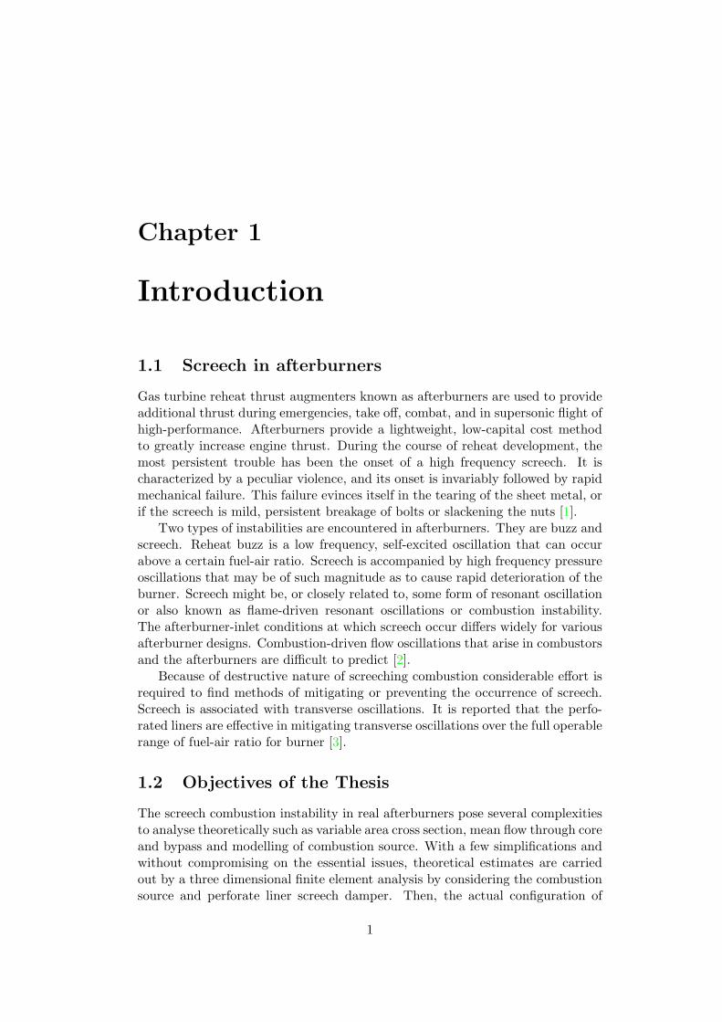
Figure 1.1: Components of the afterburner
high frequency transverse combustion instabilities.
1.3 Description and operation of the afterburner
Afterburner is an exhaust system that is fitted to the exit of low pressure turbinein the gas turbine engine. The main components of afterburner are: diffuser thatreduces the flow velocity, screech liner to attenuate the transverse oscillations, fuelmanifolds to provide proper fuel distribution and a flame stabilizer that providesthe recirculation zone for flame anchoring. Figure 1.1 shows the constructionof afterburner. Afterburner receives vitiated air from the exit of low pressureturbine (LPT) at a temperature range of 780 K to 1065 K, and a pressure rangeof 55 kPa to 380 kPa from high altitude operation to sea level. The exit velocityof LPT is of the order 0.5 to 0.6 Mach. When one desires to light up afterburnerby admitting fuel into the core cavity, it is extremely difficult or impossible toachieve a stable flame due to high incoming velocity. Hence, a diffuser is employedto reduce the velocity to the level of 0.3 Mach. A recirculation zone is created bya V-shaped bluff body. Fuel is admitted through the manifold which is situatedupstream of central V-shaped-flame-stabilizer. The catalyst (platinum-rhodium)which is located in the flame stabilizer helps in igniting the mixture of hot airfrom LPT and the fuel that is sprayed in the vaporized form through the manifoldat a pressure of 700 kPa. In the experimental test facility hot air is provided by apre-heater ahead of afterburner. At about 450C combustion is initiated. Then,all the other three manifolds are activated to achieve full afterburning at a fuelmanifolds pressure of 2720 kPa. To simulate afterburner entry conditions by thepre-heater, a fuel / air ratio in the range of 0.015 to 0.02 is needed. For fullafterburning the overall fuel air ratio is in the range of 0.05 to 0.06.
1.4. Organization of the thesis 4
1.4 Organization of the thesis
Chapter 2 gives a review of combustion instability phenomenon, amplificationmechanisms and attenuation, combustion source models and subsequently re-search carried out on afterburner systems in the past. Chapter 3 gives theoreticalformulation of the afterburner configuration that was used in the FEM analysisthrough SYSNOISE software. The coupled governing equations for acoustic anal-ysis and combustion source oscillations are derived from fundamentals. Applica-ble boundary conditions are presented. Certain simplifications are made whilepreparing the mesh from the actual geometry. The centre body, struts, and vari-able area of the test section are considered along with the perforated liner in thegeometrical modelling and a three dimensional tetrahedron mesh is created forthe purposes of analysis. The medium is considered to be with uniform acousticproperties. The other approximations and the limiting conditions appropriate tovarious regions are discussed.
A new combustion model has been proposed for obtaining the heat releaserate response function to acoustic oscillations. Acoustic wave - flame interactionsinvolve unsteady kinetic, fluid mechanic and acoustic processes over a large rangeof time scales. The development of the theory is based on large activation energyasymptotics. One-dimensional conservation equations are used for obtaining theresponse function for the heat release rate assuming the laminar flamelet modelto be valid. These are discussed in Chapter 4.
Chapter 5 presents the afterburner test facility description, capability, op-eration and the tests carried out on the (1/3)rd scale afterburner. The data isacquired by the dynamic pressure probes. Chapter 6 gives the discussion on the-oretical and experimental results. Chapter 7 gives the conclusions along withlimitations in the analysis, and difficulties encountered during experiments andthe expertise obtained in addressing screech related problems in the afterburners.
Chapter 2
Literature Survey
Combustion instabilities arise at different stages of combustion process. Thecharacteristics of such oscillatory instabilities are briefly discussed in section 2.1.Mechanism of amplification of oscillatory combustion instability is presented andthen, in section 2.2, the specific issue of instability problem in afterburners ispresented. Finally in section 2.3 the present problem definition and methodologyfollowed are discussed along with complexities involved in theoretical analysis.
2.1 Characteristics of oscillatory instabilities
The combustion instabilities are summarized into three types [4] such as:
1. Intrinsic instabilities which are inherent to the combustion and fluid physics,
2. Chamber instabilities which result from the interaction of the combustionprocess with a combustion chamber, and
3. System instabilities that involve the interaction of the combustion processesin a chamber with upstream feed lines and / or downstream exhaust.
In each of these three categories, different physical processes may contribute tothe instability. Another categorization of instabilities is in terms of the physicalprocesses involved. For example, there are buoyant instabilities, hydrodynamicinstabilities and acoustic instabilities, among others.
The oscillatory instability in gas-turbine combustors as well as afterburnersarise from the coupling of unsteady heat release with acoustic waves in a chamber,resulting in repeated pressure fluctuations at various characteristic frequencies.The instability frequencies are associated with the geometry of the device andmay be influenced by interactions between the device and flow field. The interac-tions causing these self-excited oscillations are complex because of the couplingof the flow field with unsteady (and highly non-linear) heat release. Some experi-ments have been interpreted [5,6] to indicate that a primary cause for generationof instabilities is an acoustic wave generated by unsteady heat release that tripsa Kelvin-Helmoltz instability in the flow [7], where high density gradients, shear,and substantial vortices exist. The instability modifies both the overall flame
5
2.1. Characteristics of oscillatory instabilities 6
structure and flow (turbulence), and hence an effective closed-loop feedback sys-tem is generated.
In 1878 Rayleigh proposed a criterion that has evolved into a clear rule for thepotential amplification of an acoustic wave in combustion system, essentially thatpositive correlation of the heat-release and pressure variations over the period ofone acoustic cycle results in amplification of oscillations [8],∫ T
0p′(t)q′(t) dt > 0 (2.1)
where p′ and q′ are the pressure and heat-release perturbations, respectively, asfunction of time t, and T denotes the period of the oscillation. Unfortunately,it is difficult to apply these criteria in a practical setting, as may be observed instudies [9, 10,11] of one-dimensional systems designed to model reheat buzz.
Several mechanisms have been identified that contribute to acoustic instabilityamplification, some of which are:
1. Air/ fuel ratio fluctuations which was recently investigated by Lieuwen andCho [12] resulting in heat-release perturbations at the flame can causeacoustic waves to propagate upstream into the feed lines and cause per-turbations in the incoming air/fuel mixture. These perturbations may becarried by the mean flow and trigger a fluctuation at the base of the flame,closing the instability loop. Several studies have addressed this possiblemechanism. For example, Sacarini and Freeman [13] studied the fuel-airfluctuations in a simple duct and concluded that the strong potential ofthese fluctuations to drive instabilities justified substantial effort in miti-gating air/fuel fluctuations. In their work [14], Sacanini et al [14] defined aparameter σ as an indicator of the efficiency of mixing duct,
σ =φ′
φ
/u′
u(2.2)
where φ′
φ is the ratio of air/fuel-ratio perturbations to the mean air/fuel-
ratio, and u′
u is the ratio of velocity perturbations to the mean flow velocity.Their work focused on trying to get this parameter as close to zero aspossible, which was accomplished by improving the mixing quality of thereactants by using multiple fuel-injectors.
2. Vortices shed from the flame holder were suggested as a cause of combus-tion instabilities as early as 1956 by Rogers and Marble [15]. More recently,experimental investigation by Poinsot et al [5] looked at this as a possiblesource of combustion instability. The instability is triggered when the vor-tices shed at the flame holder entrain unburned mixture, which propagatedownstream and causes a sudden heat release at some point downstream.This triggers an acoustic wave propagating upstream, closing the feedbackloop. Culick and Magiawalla [16] investigated vortices shed from the flameholder consisting of pure products, which would impinge on obstacles down-stream (e.g. the nozzle) and cause pressure oscillations to intensify. This
2.2. Combustion instabilities in afterburners 7
investigation was of purely acoustic phenomenon with no heat-release con-tribution. Mateev and Culick [17] recently investigated the formation ofvortices behind the flame holders and their interaction with flow-field per-turbations in premixed combustors, using a newly developed quasi-steadymodel. In this model, they addressed a dump combustor in which theyassumed constant fluid properties, vortex burning as the only source of in-stability (without vortex-surface interaction), and vortex propagation at themean flow velocity. They were able to partially validate the model againstexperimental results for vortex shedding in a non-reacting oscillating coldflow. The authors cited the concern that reacting flows might behave differ-ently and that resulting vortex shedding and interaction in reacting flowsmight follow a different pattern.
3. The effect of entropy waves (the phenomenon of localized hot spots) on flow-field instabilities was suggested in early work by Chu [18], who consideredtheir influence on combustion instabilities to be minimal except at lowfrequencies. Polifke et al [19] state that since the hot spots are transportedby the mean flow (usually at low velocity), effects of entropy waves havebeen assumed to exist at low frequencies [20].
Little work has been done to include damping effects in the body of literatureon combustion instabilities. Williams [4] presented some of the possible dampingsources in an oscillating combustor environment. They are wall damping, particledamping, relaxation damping, homogeneous damping, nozzle damping etc. Whenchoked flow conditions are met, the propagation of acoustic waves is restricted atthe nozzle and no propagation of longitudinal waves is allowed upstream from adiverging supersonic-flow section. This boundary can absorb energy dependingon the flow conditions. Other types of damping are due to perforated walls andcooling flows near the wall, and heat addition mechanisms acting out of phasewith pressure perturbations.
2.2 Combustion instabilities in afterburners
The combustion instabilities that are encountered in the Gas Turbine afterburnersare categorized into buzz and screech. Buzz is low frequency combustion insta-bility involving the propagation of low frequency longitudinal acoustic waves inthe duct, where as screech is associated with high frequency tangential acous-tic waves. Quite a few authors have attempted to address the problem of buzzby analytical methods and experiments in laboratory test rigs. In this section,research pertaining to low frequency combustion instability is discussed.
Dowling and Bloxidge [21] were the first to develop a theory to describe theonset of buzz in ducts with simple geometry and to determine the frequency ofunstable oscillations. This paper is discussed in detail as it formed basis for allsubsequent investigators who worked in the area of low frequency combustion os-cillations. The authors have drawn a conclusion from the schileren photographsthat the longitudinal pressure waves perturbed the flame, causing the flame tomove and change in flame surface area, thereby altering the instantaneous heat
2.2. Combustion instabilities in afterburners 8
release rate. To model this phenomenon, a control volume analysis is performedby which flame zone perturbations in heat release rate are related to the upstreamconditions. Equations for upstream and downstream condition of the flame for theperturbations of pressure, velocity, density and temperature are set up. Boundaryconditions are : i) choked flow at entry, ii) Howes reflection coefficient criteria,iii) conservation relations across the flame. Third boundary condition accommo-dates, heat release where flame surface and velocity of the element of flame aretaken into consideration. By the application of momentum conservation acrossthe control volume, the form drag of flame stabilizer is considered. As combustionconverts the chemical energy into tangible form, the linearized equation of energyconservation is written. The relationship between the unsteadiness in combus-tion and the velocity perturbation has been deduced by heuristic argument andthe same is substituted in the energy equation. Thus six homogeneous equationsfor six unknowns are set up. The unknowns are the amplitudes of incident andreflected waves from flame at upstream and downstream, heat release rate andthe acoustic wave amplitude of the convected hot spot. The sustaining unstableacoustic wave frequency is deduced for which the determinant of the above ma-trix vanishes. Computations are made for single unstable frequency for variousequivalence ratios. The predicted buzz frequency is compared with experimentaldata. At the buzz frequency by numerical method heat release rate magnitudeand phase are predicted. The author proposed that there is a need to refine theflame model that is proposed in the theory by experiments.
Bloxidge et al [10] have provided rigorous theoretical treatment to the aboveproblem. By the support of extensive experimentation on the same test rig,the flame model is described. They have assumed the rate of heat release tobe proportional to the measured light emission from radicals. Flame stabilizerblockage is neglected. By an iterative procedure buzz frequency is predictedand compared with the experimentally obtained value and there was very closeagreement.
The influence of a twin stream supply on acoustically coupled combustionoscillations was investigated by Macquisten and Dowling [22]. The duct lengthwas 0.95 m with rectangular cross section of 70×70 mm. Ethylene was used as thefuel. Inlet flow velocities are of order 0.14 Mach. Inlet temperature is 290 K forthe bypass flow and 540 K for the core flow. Only the longitudinal low frequencieswere captured. The fundamental frequency is about 109 Hz. The onset of lowfrequency combustion instabilities was predicted by linear stability analysis byhaving a relationship between velocity perturbations at the flame holder andinstantaneous heat release rate, which was derived from schlieren photographs.Though the bypass flow was simulated, the two streams were mixed in front of theflame stabilizer, thus having the same temperature. The cross-section of the testsection is rectangular. Only the longitudinal modes were studied. It is knownthat the transverse modes differ widely if the duct cross-section is rectangularinstead of circular as in the normal case.
The influence of geometric and flow variables on combustion instability inconfined flames stabilized behind a disk was examined by Sivasegaram et al [23].Core and bypass flows were simulated. Length of the duct was 480 mm and the
2.2. Combustion instabilities in afterburners 9
diameter of the duct 80 mm. Propane was used as fuel. Mean velocities upstreamof flame holder was in the range of 6.5 m/s to 11.5 m/s. Only oscillations thatwere associated with longitudinal wave frequencies of the order 150 Hz to 200 Hzware investigated. The studies were conducted with and without exit nozzles.The mass flow conditions are quite small when compared with the present trend.The study has not included the presence of perforate liner.
Dowling [24] has summarized the work related to buzz in afterburners inThe 1999 Lanchester lecture. The governing equation for coupled combustioninstability is described by the following inhomogeneous wave equation 2.3,
1c∗2
∂2p′
∂t∗2−∇2p′ =
(γ − 1)c∗2
(∂q′
∂t∗
)(2.3)
The term on the right hand side describing how the unsteady addition of heatgenerates pressure disturbances. The status of the afterburner can be summarizedas follows.
1. When equation 2.3 reduces to homogeneous wave equation whose solutionsgive the usual organ pipe modes. For the one dimensional case, by themethod of separation of varuables in the form of p′(z, t) = F (t)G(z), withthe boundary condition of zero pressure variation at z = 0 and z = l leadsto G(z) = sin(nπ/l) and F (t) = F0 sin(ωnt+φ) where ωn = nπc∗/l, n is aninteger, and F0 and φ are constants determined by the initial conditions.These solutions represent the normal organ pipe modes of oscillation withthe pressure fluctuates without decay at the resonant frequencies nπc∗/l.
2. A few combustion models are discussed to bring out the influence of un-steady heat release rate q′(z, t) on the above pressure perturbations. Onemodel suggested has the form q′ = −αc∗2
γ−1 p′, where α is a complex quan-
tity which accounts for the phase difference between the pressure and heatrelease perturbations. The boundary conditions ensure that G(z) has thesame form and the solution is given by p′(z, t) = F (t) sin(nπz/l). By thesubstitution into Eq. 2.3, 1
c∗ F+αF+ n2π2
l2F = 0 is obtained which describes
a damped oscillator. If p′ and q′ are 180 out of phase, the constant α is realand positive and describes damped oscillations. If, however, p′ and q′ are inphase α is real and negative and the solution grows in time. Thus Rayleighcriterion is recovered. Heat addition in phase with pressure perturbation isrequired for energy input into acoustic waves.
3. The second model suggested is: q′ = βγ−1
∂p′
∂t . By the substitution into
governing inhomogeneous equation, (1−β)c∗ F + n2π2
l2F = 0 is obtained. This
has no damping term, instead the interaction between heat release andpressure leads to a frequency shift. If q′ leads p′ by 1
4 cycle, β is positiveand frequency increases. If, however, q′ lags p′ by 1
4 cycle, β is negative andthe frequency decreases.
4. The examples considered above are over simplification of what occurs inpractice. Bloxidge et al [10] studied the coupled combustion instability
2.2. Combustion instabilities in afterburners 10
by extensive experiments over a wide range of equivalence ratios. Thedistribution of heat release was determined through measurements of thelight emission from C2 radicals. They obtained an emperical correlation ofthe form
q(z)q(z)
=1
1 + jω(2πr/u)u
u(2.4)
The flame model suggested in this work is purely empirical and was de-duced by simply expressing experimental results in an appropriate non-dimensional form.
5. Dowling [25] has developed a kinematic flame model, in which flame surfacearea propagates with turbulent burning velocity, Su, and q(z)
q(z) = f(u′
u , Su
).
6. Brookes et al [26] studied flame response through CFD by simulating theresults obtained by Bloxidge et al [10]. CFD model is based on laminarflamelets, the reaction rate being obtained from the product of laminarflame speed and a flame surface density function.
7. Fannin [27] has developed coupled combustion oscillation model. He per-formed control volume analysis in order to determine how the velocity per-turbations in the acoustic field would affect the overall heat release rate.The unsteadiness is described by conservation of species and energy in thecontrol volume and the heat release rate was computed as the change insensible enthalpy from the reactant flow entering to products exiting thecontrol volume. The species consist of fuel, air, and products. The volumeis assumed to be steady, but the mass fraction of species and temperatureof the control volume are allowed to vary. Single step Arhenius kineticsdescribe the rate of change of reactant and products species in the con-trol volume. The species are assumed to be perfectly and instantaneouslymixed.
As early as 1950s, extensive research have been conducted in the area ofscreech through expensive experiments, that has appeared in the literature.
Edwards [1] has reported the occurrence of screech in the tests conducted atthe National Gas Turbine Establishments. The amplitude of screech oscillationscould be as high as 40 kPa. And the fundamental screech modes range between250 Hz to 750 Hz and 450 Hz to 1300 Hz for the first harmonic transverse modesdepending upon the temperature of the gases.
Lundin et al [3] have conducted experiments on straight jet afterburners whoseinlet velocities are in the rage of 0.32 Mach, and inlet pressure 150 kPa. Aperforated liner with 4.75 mm diameter holes was installed concentrically withthe afterburner. Fuel injection was by 24 spray bars, and flame stabilization wasachieved with the help of two concentric V-shaped stabilizers. Two configurationsare considered with L/D ratio of combustion volume 2.3 and 4.2. A screechfrequency of 650 Hz was encountered. The first and the fourth transverse modeswere encountered. Screech holes were spread up to 915 mm from the flamreholder. With the perforated liner, screech was completely eliminated. It may be
2.2. Combustion instabilities in afterburners 11
noted here that straight jet engines are replaced by small bypass engines and thelatest engines operate at much higher pressures and in the absence of theoreticalestimates, a lot of effort and time are required in the experiments to identify thescreech frequencies.
The investigation of combustion instability was conducted by James et al[28] in two separate test facilities, a 26 inch-diameter duct rig and a 32-inch-diameter short afterburner attached to a full-scale turbojet engine. Spray barsand diametrical flame holder are used. Exit nozzle was not fitted and bypassflow was not simulated in the rig testing. Inlet temperature is 950 K. L/D ofcombustion volume is 2.8. First transverse mode of oscillation occurred at 635Hz. In the 32 inch diameter afterburner a perforated liner was used. The bypassair around the perforated liner was also at 950 K. In this case bypass and coreflow are at the same temperature. Several configurations were tested in the rig.
The Lewis Laboratory staff [2] have summarized all the preliminary investi-gations in the area of combustion screech. All of the work is based on exper-iments. Several straight jet afterburner configurations data was presented. Itis observed that without the perforated screech liner, at all equivalence ratios,screech commenced. With the perforated liner, screech occurred only very closeto stoichiometric condition or eliminated completely.
There was a long silence on the subject after the 1950s. Increasing demandsfor higher afterburner performance of late have required operation at progres-sively higher fuel-air ratios, which has increased the occurrence and intensity ofscreeching combustion.
Much of earlier works primarily dealt with reheat buzz that occur at low fre-quencies and tested at low capacity test rigs. In these tests, the actual afterburnerconfigurations were not considered. Though full size afterburners for screech wereinvestigated in 1950s, they were straight jet low thrust engines without bypassflow. Though every engine manufacturer studies the problem of screech, beforefinalization of the design, the information remains classified. Thus there is a sig-nificant requirement of performing analysis a priori to identify screech frequenciesin real afterburners and provide a method to mitigate screech that could help inthe finalization of the afterburner design for the modern gas turbine engines.Having theoretical estimates, one can undertake only confirmatory experimentaltests and save a lot of time and effort.
Main conclusions drawn from the above study of literature are as follows:
1. Combustion instability problem is dealt for low frequency longitudinal modesof oscillations namely reheat buzz by theory and test rig level at very lowflow conditions.
2. Combustion models developed are based on flame surface area and velocityfluctuations, which are at best valid under quasi-steady conditions.
3. In the area of screech, which is a high frequency transverse oscillation,only experimental data is reported for the straight jet engines. No rigoroustheoretical analysis is reported.
Pressure wave-flame interaction is a very important phenomenon in after-burners due to flame acceleration and turbulent break up of laminar flames.A
2.2. Combustion instabilities in afterburners 12
comprehensive review of physics of oscillatory combustion in Gas Turbines iswell documented by Ibrahim et al [29]. Besides describing the characteristics,amplification, damping of oscillatory instabilities, the authors suggested possiblemethods of theoretical study including unsteady computational fluid dynamicssimulation. Hathout [30], Ducruix et al [31], Keller [32], Bellucci et al [33],Dowling and Stow [34], Searby and Rochwerger [35], Culick [36], Lee and San-tavicca [37], Lieuwen [38], and Fleifil [39] are some of the main authors whohave explained the phenomenon of pressure wave-flame interactions leading tocombustion instability elaborately.In this regard, Jean Pierre has derived Raleighcriterion analytically. Ducruix has derived governing equations for combustioninstability by incorporating reaction kinetics due to heat release. However noestimates are made. Dowling has suggested few simple models for heat releaserate fluctuation computation.
Particular interest in the present work is to consider chemical kinetics ofreaction in the combustion zone and to see how acoustic pressure couple withheat release fluctuations in the frequency range of 100– 1500 Hz.
Clarke [40] discussed the pressure flame interaction at more fundamental level.The work that is having lot of similarities with present thesis in respect of acous-tic combustion source characterization is due to McIntosh [41]. Using time andlength scale ratios McIntosh gave mathematical treatment for modelling combus-tion heat release response function. Acoustic wave lengths of interest in combus-tion systems is in the range of 10−2 to 100 m , flame response time scale is 10−3
to 10−2 s [42]. Mach number, M is of the flame burning velocity of the order10−4 and Θ is of the order 10 (dimensionless overall activation energy).
McIntosh [41] has proposed three distinct cases of pressure - premixed flameinteractions based on the time scales of the various processes.
1. Low amplitude coupling (δ ∼ O(M), time scale≈ 1 i.e. medium wave lengthof the order 3500 Hz): In this the assumption is coupling is through velocityperturbation. This is significant only when heat loss comes into effect. Inafterburners that is not relevant. Moreover such low level acoustics simplyregarded the flame as a contact discontinuity swept along with a smallunsteady acoustics. In such case pressure gradients do not exist in thecombustion zone. That is to say that inner reaction zone is not affected bypressure field. The effect of presence of disturbances is predominantly inthe outer combustion zones which are swept away. Under the assumptionof small amplitude, δ ∼ O(M), there was no coupling of pressure changeswith the temperature disturbances at the flame.
2. When δ is raised to the level of Θ−1 coupling can occur. For large wavelengths (time scale << 1) van Harten et al [43] included density effects andfor medium wave lengths (time scale ≈ 1) density effects were not included.Here also no pressure gradients are felt in the combustion zone. The after-burner combustion experiences large wavelength (buzz) and medium wavelength (screech) combustion instability.
3. Very high frequency waves: (time scale ≈ M−1) In such cases for largeamplitudes of coupling (δ ≈ Θ−1), non linearities develop which are much
2.3. Problem definition — Scope of analysis and testing 13
affected by the sharp density changes through the flame. Here pressuregradients are very important in the combustion zone which contains thefull effect of any pressure wave passing through. It results in non-constantwave speed with non linearities for large amplitude disturbances.
McIntosh [41] has given formulation of above phenomenon by the equations ofstate, continuity, energy, species and momentum equations. The important as-sumption is density times thermal conductivity is a constant. It implies thatthe thermal conductivity is proportional to temperature which is experimentallyfound. This assumption also simplifies energy and species equations. By classicallarge activation energy analysis linear acoustic relations are derived for reactionzone and Eulerian equations for upstream and downstream of combustion zone.These equations are similar, but not identical to those of van Harten et al [43].The major difference is that in their work, they assumed constant thermal con-ductivity and derived non linear partial differential equations, the non linearityarising out of the density effects. In McIntosh [41] work neither thermal con-ductivity nor density is assumed constant. By assuming harmonic inputs fortemperature, chemical mixture concentration, mass flux and pressure, equationsare linearized and then mass flux perturbation quantity was computed in thecase of medium wave lengths for Lewis numbers 0.3, 0.5, 1.0 and 1.5. The mainconclusion was that the fluctuations are roughly twice as large from the reactionzone side as those with unburnt upstream side.
In the present work, a new heat release response function due to acousticpressure perturbations is developed from the fundamental equations and resultsare compared with the work of McIntosh [41] highlighting the similarities anddifferences in chapter 4.
2.3 Problem definition — Scope of analysis and test-ing
The real afterburners pose several complexities to analyze theoretically, such asvariable area cross section, mean flow through core and bypass and unsteady re-sponse of combustion source. Early studies of acoustic wave oscillations throughvariable area ducts restricted their scope to the case of no mean flow. Severalresearchers have obtained the wave propagation solutions in ducts whose wallsvary sinusoidally [44, 45, 46, 47, 48]. Others have used a discretization techniquebased on the solution for a single duct discontinuity [49, 50, 51]. The inclusionof the effects of a mean flow to provide more realistic model makes the problemconsiderably more difficult, and most studies have employed one or more simpli-fying assumptions. Some have used the assumption of one-dimensional flow andrestricted their analysis to the propagation of the lowest acoustic mode throughducts with variable cross sections [52, 53]. However, the restrictions to propaga-tion of the fundamental mode limit the usefulness of such analyses for realisticsituations in which the sound is a combination of numerous modes (longitudinal,tangential and radial). For ducts with larger axial variations, coupling betweenmodes will occur [54,55,56,57].
2.3. Problem definition — Scope of analysis and testing 14
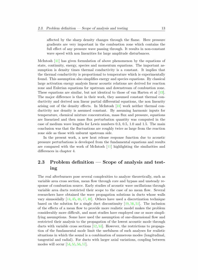
Figure 2.1: Method of study of combustion oscillatory instabilities
Although there was considerable effort in the development of analytical andnumerical methods to predict acoustic wave propagation in variable area ducts,combustion source modelling is not included especially for identifying the screechfrequencies along with the influence of perforate liner to mitigate screech fre-quency amplitude. For this reason, theoretical estimates are carried out by athree dimensional finite element analysis by considering the combustion sourceoscillations and perforate liner. Figure 2.1 shows the block diagram in which,the methodology followed in the present work to study the high frequency com-bustion instability is presented. The governing equations describing the acoustic
2.3. Problem definition — Scope of analysis and testing 15
phenomenon due to combustion are derived. Finite element formulation is de-scribed along with boundary conditions. The equations are coupled with heatrelease. A new combustion model has been proposed for obtaining the heat releaserate response function. As discussed earlier the heat release response functionscurrently explored in the literature are based on mixture ratio variation and/orflame surface area variation. These are quasi-steady models applicable to onlylow frequency oscillations.
Most of the previous work were focused on the longitudinal mode of oscilla-tions at relatively low frequencies. These models are not applicable to the currentwork, which primarily deals with transverse modes at high frequencies (up toabout 2000 Hz). Since pressure directly affects the reaction rates, the classicallaminar flame approach has been adapted for developing the heat release responsefunction. The combustion related sound pressure level as a function of frequencyis applied at various locations in the afterburner flame stabilizer zone and thesolution is obtained by available software. The coupling of flame and acousticoscillations is expected to amplify the amplitude of pressure oscillations and thepresence of perforate liner will attenuate the same by certain percentage. In theafterburners passive control of combustion instabilities is by the use of liners. Cer-tain percentage of attenuation is achieved by drilling holes on the liner that willreduce acoustic energy from the combustion chambers that would otherwise re-turn to the coupling mechanism of the feed back loop [58,59,60]. Mechel [61,62]has suggested modelling methods to estimate perforate liner impedance. Thecomplex liner impedance is modelled and implemented in the software whereliner is located to assess the attenuation characteristics of combustion instabil-ities. Mechel [63] has provided a comprehensive review and compilation of thework on liners and has presented the formulae on different types of liners. Thepresent work utilizes the formulae suggested in this reference to model the acous-tic liner. The details of the theoretical formulation with appropriate boundaryconditions are presented in chapters 3 and 4.
The actual configuration of afterburner was tested for confirmation of identi-fied screech frequencies and that their amplitudes do not overshoot the permissi-ble limits for the safe afterburner operation.
Chapter 3
Theory
In this chapter, the governing equations for the acoustic response of the after-burner by inclusion of combustion source are derived. Subsequently, boundaryconditions, at inlet and at outlet of test section, acoustic impedance boundarycondition that characterizes the screech liner, and exit nozzle admittance arepresented. The Mathematical treatment is presented for completion.
3.1 The Governing Equations
The afterburner is essentially having two sections. In the first portion, the com-bustion process is considered as a reacting mixture flowing in a constant area ductwith a flame anchored at a specific location in the duct. When the reactants areignited, chemical energy is released in the form of heat, thus raising temperatureof the flowing fluid. In the second section the burnt products are acceleratedin the convergent nozzle to sonic velocity at throat. This type of combustionprocess sustains acoustic pressure and velocity oscillations. The flow in the after-burner, not only have inherent instabilities, but also respond readily to imposedfluctuations. Thus, the potential coupling between the unsteady components ofpressure and heat release rate leads to their resonant coupling and growth. Thisphenomenon is referred to as thermoacoustic instability.
In the following section, equations governing the acoustic pressure and veloc-ity are obtained in the presence of unsteady heat addition within the afterburner.These are manipulated to get the forced acoustic wave equation which is then re-duced to the case when the mean heat release is negligible, that is, approximatelyhomogeneous field, and when the mean flow is negligible.
The flow of gases in each of the two regions is governed by the well knownNavier-Stokes equations. The basic assumptions used for the flow in the after-burner are:
1. three dimensional flow
2. inviscid flow, that is, the duct has negligible dissipation effect on the acous-tic waves,
3. negligible thermal conduction to the surroundings.
16
3.1. The Governing Equations 17
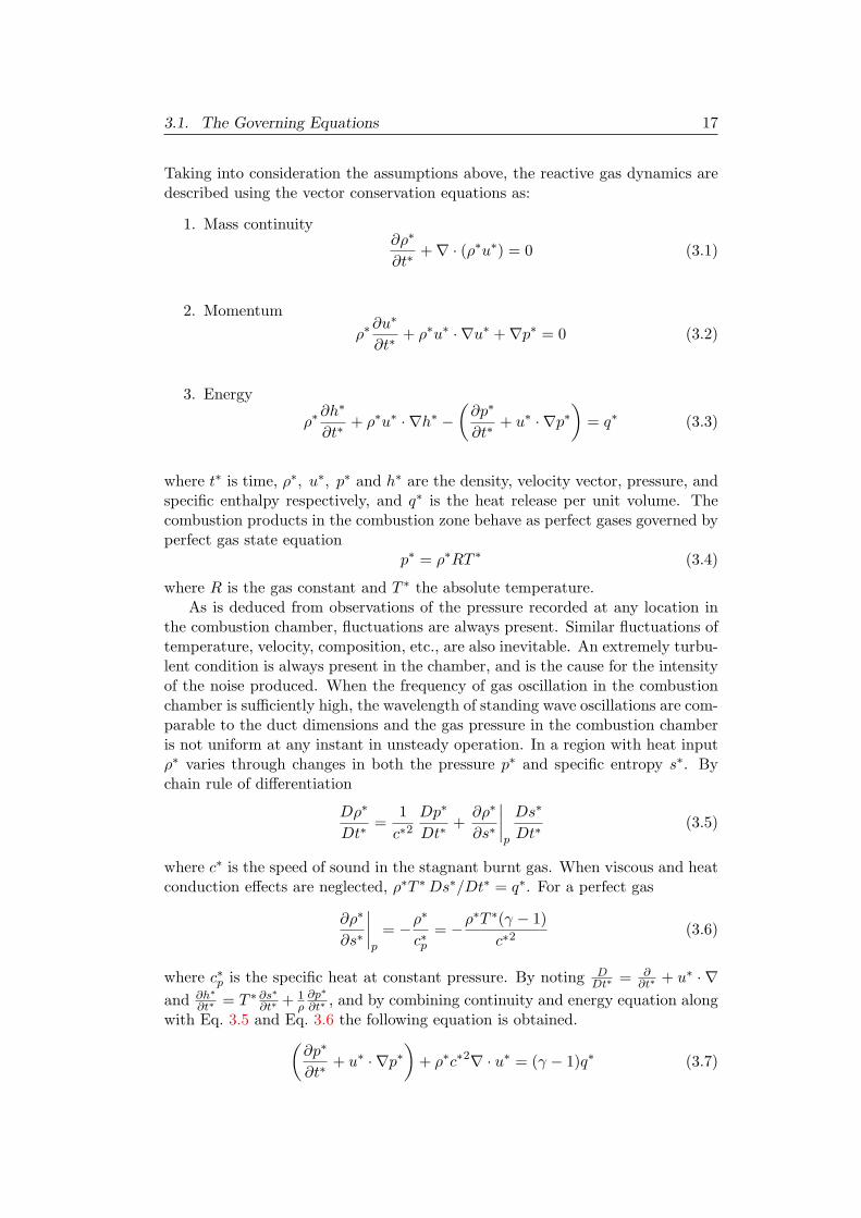
Taking into consideration the assumptions above, the reactive gas dynamics aredescribed using the vector conservation equations as:
1. Mass continuity∂ρ∗
∂t∗+∇ · (ρ∗u∗) = 0 (3.1)
2. Momentumρ∗∂u∗
∂t∗+ ρ∗u∗ · ∇u∗ +∇p∗ = 0 (3.2)
3. Energy
ρ∗∂h∗
∂t∗+ ρ∗u∗ · ∇h∗ −
(∂p∗
∂t∗+ u∗ · ∇p∗
)= q∗ (3.3)
where t∗ is time, ρ∗, u∗, p∗ and h∗ are the density, velocity vector, pressure, andspecific enthalpy respectively, and q∗ is the heat release per unit volume. Thecombustion products in the combustion zone behave as perfect gases governed byperfect gas state equation
p∗ = ρ∗RT ∗ (3.4)
where R is the gas constant and T ∗ the absolute temperature.As is deduced from observations of the pressure recorded at any location in
the combustion chamber, fluctuations are always present. Similar fluctuations oftemperature, velocity, composition, etc., are also inevitable. An extremely turbu-lent condition is always present in the chamber, and is the cause for the intensityof the noise produced. When the frequency of gas oscillation in the combustionchamber is sufficiently high, the wavelength of standing wave oscillations are com-parable to the duct dimensions and the gas pressure in the combustion chamberis not uniform at any instant in unsteady operation. In a region with heat inputρ∗ varies through changes in both the pressure p∗ and specific entropy s∗. Bychain rule of differentiation
Dρ∗
Dt∗=
1c∗2
Dp∗
Dt∗+∂ρ∗
∂s∗
∣∣∣∣p
Ds∗
Dt∗(3.5)
where c∗ is the speed of sound in the stagnant burnt gas. When viscous and heatconduction effects are neglected, ρ∗T ∗Ds∗/Dt∗ = q∗. For a perfect gas
∂ρ∗
∂s∗
∣∣∣∣p
= −ρ∗
c∗p= −ρ
∗T ∗(γ − 1)c∗2
(3.6)
where c∗p is the specific heat at constant pressure. By noting DDt∗ = ∂
∂t∗ + u∗ · ∇and ∂h∗
∂t∗ = T ∗ ∂s∗
∂t∗ + 1ρ∂p∗
∂t∗ , and by combining continuity and energy equation alongwith Eq. 3.5 and Eq. 3.6 the following equation is obtained.(
∂p∗
∂t∗+ u∗ · ∇p∗
)+ ρ∗c∗2∇ · u∗ = (γ − 1)q∗ (3.7)
3.1. The Governing Equations 18
The above equations can be applied to a combusting gas, assuming that thereactants and products behave as perfect gases and that there is no molecularmass change during chemical reaction.
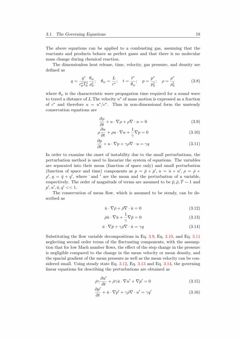
The dimensionless heat release, time, velocity, gas pressure, and density aredefined as
q =q∗
c∗pT∗0
θwρ∗0
; θw =L
c∗; t =
t∗
θw; p =
p∗
p∗0; ρ =
ρ∗
ρ∗0(3.8)
where θw is the characteristic wave propagation time required for a sound waveto travel a distance of L.The velocity u∗ of mass motion is expressed as a fractionof c∗ and therefore u = u∗/c∗. Thus in non-dimensional form the unsteadyconservation equations are
∂ρ
∂t+ u · ∇ρ+ ρ∇ · u = 0 (3.9)
ρ∂u
∂t+ ρu · ∇u+
1γ∇p = 0 (3.10)
∂p
∂t+ u · ∇p+ γρ∇ · u = γq (3.11)
In order to examine the onset of instability due to the small perturbations, theperturbation method is used to linearize the system of equations. The variablesare separated into their mean (function of space only) and small perturbation(function of space and time) components as p = p + p′, u = u + u′, ρ = ρ +ρ′, q = q + q′, where ¯ and ′ are the mean and the perturbation of a variable,respectively. The order of magnitude of terms are assumed to be p, ρ, T ∼ 1 andp′, u′, u, q′ << 1.
The conservation of mean flow, which is assumed to be steady, can be de-scribed as
u · ∇ρ+ ρ∇ · u = 0 (3.12)
ρu · ∇u+1γ∇p = 0 (3.13)
u · ∇p+ γρ∇ · u = γq (3.14)
Substituting the flow variable decompositions in Eq. 3.9, Eq. 3.10, and Eq. 3.11neglecting second order terms of the fluctuating components, with the assump-tion that for low Mach number flows, the effect of the step change in the pressureis negligible compared to the change in the mean velocity or mean density, andthe spacial gradient of the mean pressure as well as the mean velocity can be con-sidered small. Using steady state Eq. 3.12, Eq. 3.13 and Eq. 3.14, the governinglinear equations for describing the perturbations are obtained as
ργ∂u′
∂t+ ργu · ∇u′ +∇p′ = 0 (3.15)
∂p′
∂t+ u · ∇p′ + γρ∇ · u′ = γq′ (3.16)
3.1. The Governing Equations 19
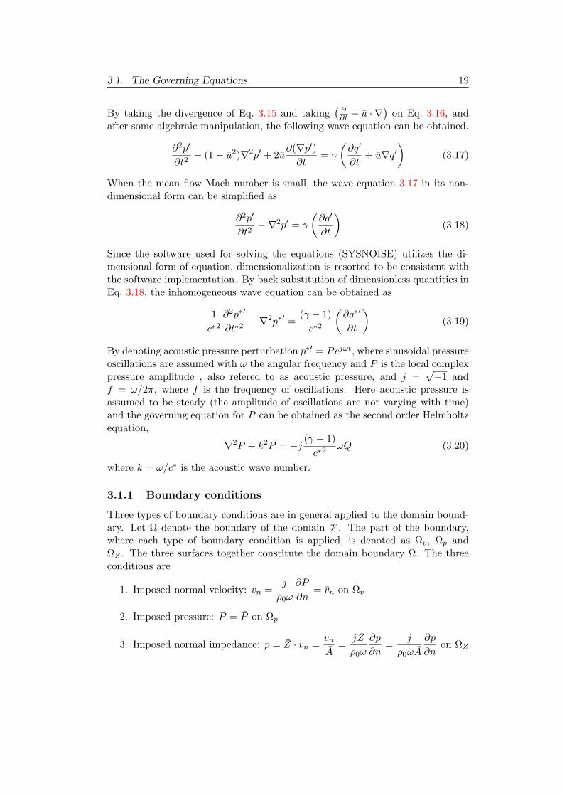
By taking the divergence of Eq. 3.15 and taking(∂∂t + u · ∇
)on Eq. 3.16, and
after some algebraic manipulation, the following wave equation can be obtained.
∂2p′
∂t2− (1− u2)∇2p′ + 2u
∂(∇p′)∂t
= γ
(∂q′
∂t+ u∇q′
)(3.17)
When the mean flow Mach number is small, the wave equation 3.17 in its non-dimensional form can be simplified as
∂2p′
∂t2−∇2p′ = γ
(∂q′
∂t
)(3.18)
Since the software used for solving the equations (SYSNOISE) utilizes the di-mensional form of equation, dimensionalization is resorted to be consistent withthe software implementation. By back substitution of dimensionless quantities inEq. 3.18, the inhomogeneous wave equation can be obtained as
1c∗2
∂2p∗′
∂t∗2−∇2p∗′ =
(γ − 1)c∗2
(∂q∗′
∂t
)(3.19)
By denoting acoustic pressure perturbation p∗′ = Pejωt, where sinusoidal pressureoscillations are assumed with ω the angular frequency and P is the local complexpressure amplitude , also refered to as acoustic pressure, and j =
√−1 and
f = ω/2π, where f is the frequency of oscillations. Here acoustic pressure isassumed to be steady (the amplitude of oscillations are not varying with time)and the governing equation for P can be obtained as the second order Helmholtzequation,
∇2P + k2P = −j (γ − 1)c∗2
ωQ (3.20)
where k = ω/c∗ is the acoustic wave number.
3.1.1 Boundary conditions
Three types of boundary conditions are in general applied to the domain bound-ary. Let Ω denote the boundary of the domain V . The part of the boundary,where each type of boundary condition is applied, is denoted as Ωv, Ωp andΩZ . The three surfaces together constitute the domain boundary Ω. The threeconditions are
1. Imposed normal velocity: vn =j
ρ0ω
∂P
∂n= vn on Ωv
2. Imposed pressure: P = P on Ωp
3. Imposed normal impedance: p = Z · vn =vnA
=jZ
ρ0ω
∂p
∂n=
j
ρ0ωA
∂p
∂non ΩZ
3.1. The Governing Equations 20
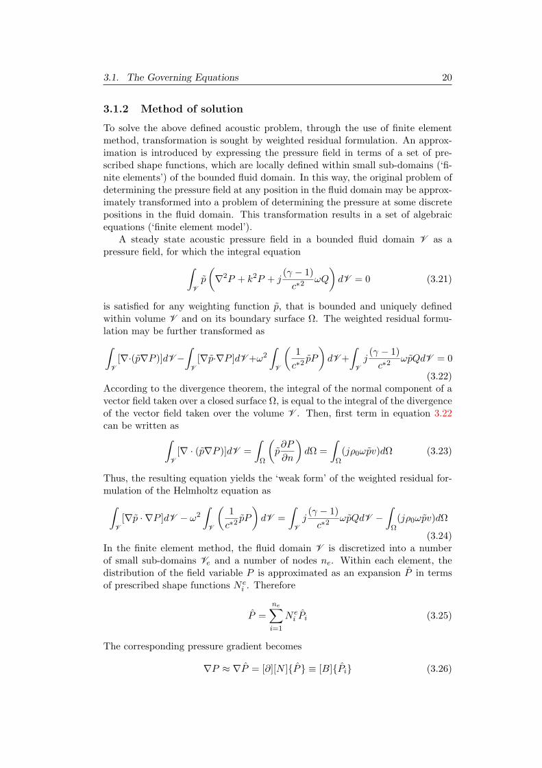
3.1.2 Method of solution
To solve the above defined acoustic problem, through the use of finite elementmethod, transformation is sought by weighted residual formulation. An approx-imation is introduced by expressing the pressure field in terms of a set of pre-scribed shape functions, which are locally defined within small sub-domains (‘fi-nite elements’) of the bounded fluid domain. In this way, the original problem ofdetermining the pressure field at any position in the fluid domain may be approx-imately transformed into a problem of determining the pressure at some discretepositions in the fluid domain. This transformation results in a set of algebraicequations (‘finite element model’).
A steady state acoustic pressure field in a bounded fluid domain V as apressure field, for which the integral equation∫
Vp
(∇2P + k2P + j
(γ − 1)c∗2
ωQ
)dV = 0 (3.21)
is satisfied for any weighting function p, that is bounded and uniquely definedwithin volume V and on its boundary surface Ω. The weighted residual formu-lation may be further transformed as∫
V[∇·(p∇P )]dV −
∫V
[∇p·∇P ]dV +ω2
∫V
(1c∗2
pP
)dV +
∫Vj
(γ − 1)c∗2
ωpQdV = 0
(3.22)According to the divergence theorem, the integral of the normal component of avector field taken over a closed surface Ω, is equal to the integral of the divergenceof the vector field taken over the volume V . Then, first term in equation 3.22can be written as∫
V[∇ · (p∇P )]dV =
∫Ω
(p∂P
∂n
)dΩ =
∫Ω
(jρ0ωpv)dΩ (3.23)
Thus, the resulting equation yields the ‘weak form’ of the weighted residual for-mulation of the Helmholtz equation as∫
V[∇p · ∇P ]dV − ω2
∫V
(1c∗2
pP
)dV =
∫Vj
(γ − 1)c∗2
ωpQdV −∫
Ω(jρ0ωpv)dΩ
(3.24)In the finite element method, the fluid domain V is discretized into a numberof small sub-domains Ve and a number of nodes ne. Within each element, thedistribution of the field variable P is approximated as an expansion P in termsof prescribed shape functions N e
i . Therefore
P =ne∑i=1
N ei Pi (3.25)
The corresponding pressure gradient becomes
∇P ≈ ∇P = [∂][N ]P ≡ [B]Pi (3.26)
3.1. The Governing Equations 21
The first term of Eq. 3.24 yields∫V
[∇p · ∇P ]dV = piT(∫
V[B]T · [B]dV
)Pi ≡ PiT [K]Pi (3.27)
where the matrix [K] is called the acoustic stiffness matrix. The second term ofEq. 3.24 yields
−ω2
∫V
(1c∗0
2 pP
)dV = −ω2piT
(∫V
1c∗0
2 [N ]T · [N ]dV)Pi ≡ −ω2piT [M ]Pi
(3.28)where the matrix [M ] is called the acoustic mass matrix. The third term of Eq.3.24 yields∫
Vj
(γ − 1)c∗2
ωpQdV = PiT(∫
Vj
(γ − 1)c∗2
ω[N ]TQdV)pT ≡ pT · Qi
(3.29)where Qi is known as the acoustic excitation vector.
The last term in Eq. 3.24 accommodates the introduction of boundary condi-tions. The integration over the surface may be regarded as a sum of the integra-tions over the sub-surfaces Ωv, ΩZ and Ωp.The boundary conditions of normalvelocity, normal impedance and pressure must be satisfied on the correspondingsurfaces. The last term in Eq. 3.24 may be expressed as
−∫
Ωv
(jρ0ωpv)dΩ−∫
ΩZ
(jρ0ωpv)dΩ−∫
Ωp
(jρ0ωpv)dΩ (3.30)
The terms of the above expression can be written in terms of shape functions as
−∫
Ωv
(jρ0ωpv)dΩ = pT(∫
Ωv
−jρ0ω[N ]T · vndΩ)P = piT v (3.31)
−∫
ΩZ
(jρ0ωpv)dΩ = −jωpT(∫
ΩZ
ρ0A[N ]T · [N ]dΩ)P = −jωpiT · [C] · Pi
(3.32)
−∫
Ωp
(jρ0ωpv)dΩ = pT ·
(∫Ωp
(−jρ0ω[N ]T v · n) · dΩ
)P = piT · p
(3.33)
By substituting Eq. 3.28, Eq. 3.29, Eq. 3.31, Eq. 3.32 and equation 3.33, inEq. 3.24, the weak form of the weighted residual formulation of the Helmholtzequation, including the boundary conditions becomes
piT ([K] + jω[C]− ω2[M ]) · Pi = pT · (Q+ vn+ p) (3.34)
The final equation to be solved is given by
([K] + jω[C]− ω2[M ])pi = (Q+ vn+ p) (3.35)
Equation 3.35 is the resulting finite element model for a coupled acoustic problem.The above equations are solved through SYSNOISE software.
3.2. SYSNOISE Software 22
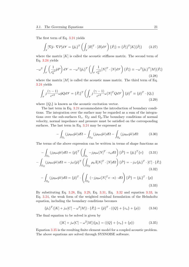
Figure 3.1: The afterburner acoustic mesh
3.2 SYSNOISE Software
SYSNOISE [64] is program for modelling acoustics and vibro-acoustics, usingthe finite element and boundary element methods. It calculates acoustic wavebehaviour in fluids, and two-way fluid-structure interaction, using implementa-tions of the finite element and boundary element methods focussed on optimalsolutions for acoustic problems. The acoustic domain can be closed, open, orpartially-open, including homogeneous fluid or multiple fluids. A coupled struc-ture can be wholly or partly connected to fluid.
SYSNOISE predicts the sound wave propagation. It calculates a wide varietyof results such as sound pressure and radiated sound power, acoustic velocitiesand intensities, contributions of panel groups to the sound, energy densities,vibro-acoustic sensitivities, normal modes and structural deflections.
SYSNOISE utilizes numerical methods based on the direct and indirect bound-ary element method and a pressure formulation for acoustic finite and infiniteelement modelling. A finite element model represents the elasticity of the fluidloaded structure. Calculations are performed in both frequency and time do-mains.
SYSNOISE models acoustics and vibro-acoustics as a wave phenomenon. Inmost cases, the modelling is carried out in the frequency domain, thus using theHelmoltz form of the wave equation.
The Direct Response frequency analysis procedure solves the following systemof equations for selected frequencies.
([K] + jω[C]− ω2[M ])p′ = ([Q] + u′n+ p) (3.36)
Right hand side of equation 3.36 is proportional to the normal velocity boundaryconditions imposed on the faces of the mesh as well as any forcing functionthat can applied in the acoustic domain as defined by the user. The stiffness,damping and mass matrices are computed only once as they are independent ofthe frequency. At each frequency, the system of equations is set up and solved toobtain the pressure distribution.
Figure 3.1 shows the afterburner acoustic mesh that was modelled for FEMacoustic analysis. The acoustic mesh is modelled from the slave combustor exitonwards. Centre body, symmetrical struts and flame stabiliser are taken intoaccount in meshing. Bypass air column is provided where the perforate liner ispositioned.
3.3. Acoustic impedance of perforate liner geometry 23
As the main concern is to capture transverse acoustic pressure variation alongthe cross section of the afterburner, three dimensional mesh is chosen. For the testsection, the first cut on frequency in transverse direction is 847 Hz at acousticspeed of 343 m/s. This number will be even higher for the case of hot slavecombustor and afterburner. Thus the frequency of interest is chosen up to 2000 Hzin the analysis. The mesh consists of 266707 TETR4 and 2206 PENT6 elements.Numerical pollution can be avoided by 6 elements per wavelength. The meshdesign rule is
Γ <c∗
6fmax
√2πfmax
c∗
(3.37)
The maximum frequency up to which calculations are carried out is 2000 Hz,which requires Γ, element length to be 10 mm. The mesh is made still finer bychoosing element length to be 5 mm because of which the mesh is valid up to4000 Hz as the software recommends that the mesh size should be such that it isvalid up to double the frequency of interest.
In order to predict the linear response of the system subjected to harmonic ex-citation, steady state dynamic analysis is performed. The panel vibration bound-ary condition is imposed to excite the acoustic field. Particle velocity along ele-ments at inlet face edge is applied, which is considered as an open end, becausethe face is connected to a large diverging combustor inlet. With the forcing func-tion, frequency by frequency computation of complex acoustic potentials at eachnode in the mesh is carried out. By defining the panel vibration as having acomplex value of 1 + j0 m/s for the frequency range of 10 Hz to 2000 Hz, thephase response is relative to the expansion of the source into the acoustic field.
Figure 3.2 gives the normalized acoustic pressure and phase for uncoupledcase which is obtained for the given test section by inlet excitation and nozzleadmittance boundary condition. Calculations involving perforate liner impedanceand nozzle admittance are presented in section 3.3 and section 3.4 respectively.
3.3 Acoustic impedance of perforate liner geometry
In the afterburner test section the perforated liner is provided to attenuate theamplitudes of screech frequencies. A few of the perforate liner models are reviewed[65,66,67]. The acoustic impedance, Z, of perforate liner is a complex function ofseveral physical variables, namely, porosity (assumed to be uniform), mean-flowvelocity through the holes or grazing the holes, diameter and thickness. Z iscalculated by using the Mechels formula [63] which is widely used. This formulais relevant when the perforate thickness is not too large (thickness << 2d). It canbe used in the linear range. The non-linearity of the real component of Z appearswhen u′n ≥ 3
√ωµρ∗ where u′n is the particle velocity in the perforate orifice.
Z ≡ p′
u′n= Rp + jXp (3.38)
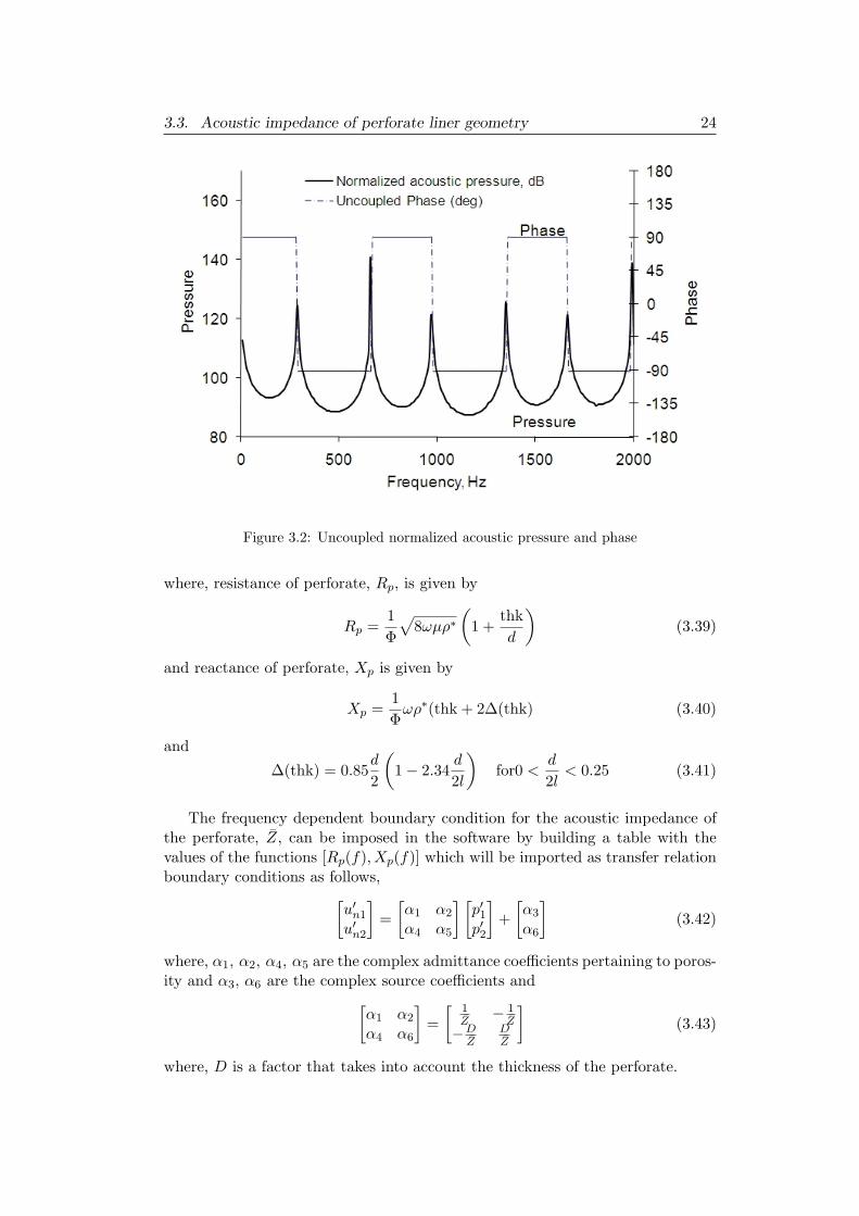
3.3. Acoustic impedance of perforate liner geometry 24
Figure 3.2: Uncoupled normalized acoustic pressure and phase
where, resistance of perforate, Rp, is given by
Rp =1Φ
√8ωµρ∗
(1 +
thkd
)(3.39)
and reactance of perforate, Xp is given by
Xp =1Φωρ∗(thk + 2∆(thk) (3.40)
and
∆(thk) = 0.85d
2
(1− 2.34
d
2l
)for0 <
d
2l< 0.25 (3.41)
The frequency dependent boundary condition for the acoustic impedance ofthe perforate, Z, can be imposed in the software by building a table with thevalues of the functions [Rp(f), Xp(f)] which will be imported as transfer relationboundary conditions as follows,[
u′n1
u′n2
]=[α1 α2
α4 α5
] [p′1p′2
]+[α3
α6
](3.42)
where, α1, α2, α4, α5 are the complex admittance coefficients pertaining to poros-ity and α3, α6 are the complex source coefficients and[
α1 α2
α4 α6
]=[ 1
Z− 1Z
−DZ
DZ
](3.43)
where, D is a factor that takes into account the thickness of the perforate.
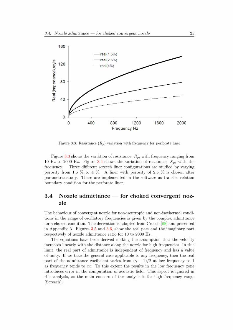
3.4. Nozzle admittance — for choked convergent nozzle 25
Figure 3.3: Resistance (Rp) variation with frequency for perforate liner
Figure 3.3 shows the variation of resistance, Rp, with frequency ranging from10 Hz to 2000 Hz. Figure 3.4 shows the variation of reactance, Xp, with thefrequency. Three different screech liner configurations are studied by varyingporosity from 1.5 % to 4 %. A liner with porosity of 2.5 % is chosen afterparametric study. These are implemented in the software as transfer relationboundary condition for the perforate liner.
3.4 Nozzle admittance — for choked convergent noz-zle
The behaviour of convergent nozzle for non-isentropic and non-isothermal condi-tions in the range of oscillatory frequencies is given by the complex admittancefor a choked condition. The derivation is adapted from Crocco [68] and presentedin Appendix A. Figures 3.5 and 3.6, show the real part and the imaginary partrespectively of nozzle admittance ratio for 10 to 2000 Hz.
The equations have been derived making the assumption that the velocityincreases linearly with the distance along the nozzle for high frequencies. In thislimit, the real part of admittance is independent of frequency and has a valueof unity. If we take the general case applicable to any frequency, then the realpart of the admittance coefficient varies from (γ − 1)/2 at low frequency to 1as frequency tends to ∞. To this extent the results in the low frequency zoneintroduces error in the computation of acoustic field. This aspect is ignored inthis analysis, as the main concern of the analysis is for high frequency range(Screech).
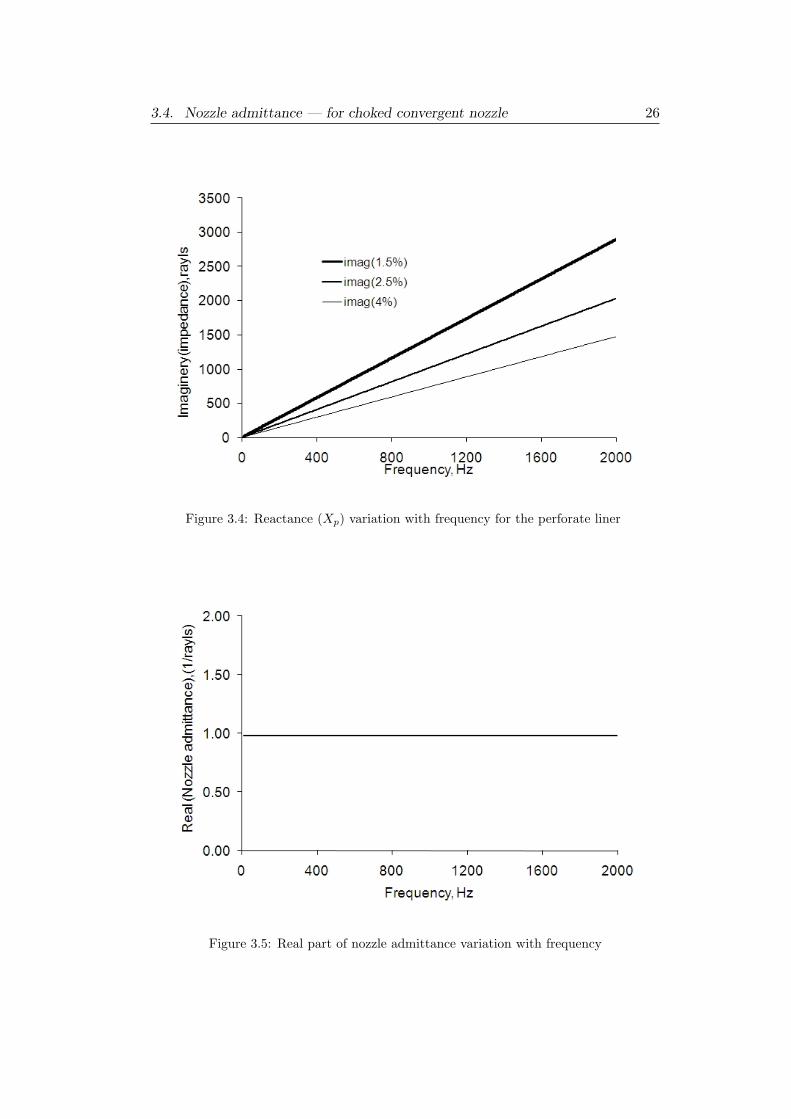
3.4. Nozzle admittance — for choked convergent nozzle 26
Figure 3.4: Reactance (Xp) variation with frequency for the perforate liner
Figure 3.5: Real part of nozzle admittance variation with frequency
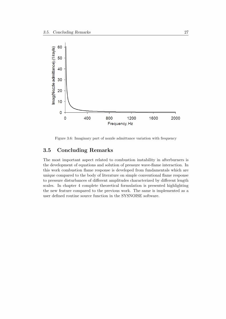
3.5. Concluding Remarks 27
Figure 3.6: Imaginary part of nozzle admittance variation with frequency
3.5 Concluding Remarks
The most important aspect related to combustion instability in afterburners isthe development of equations and solution of pressure wave-flame interaction. Inthis work combustion flame response is developed from fundamentals which areunique compared to the body of literature on simple conventional flame responseto pressure disturbances of different amplitudes characterized by different lengthscales. In chapter 4 complete theoretical formulation is presented highlightingthe new feature compared to the previous work. The same is implemented as auser defined routine source function in the SYSNOISE software.
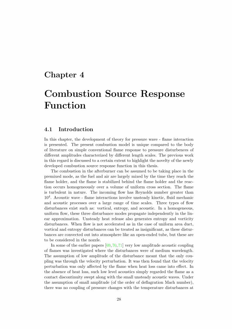
Chapter 4
Combustion Source ResponseFunction
4.1 Introduction
In this chapter, the development of theory for pressure wave - flame interactionis presented. The present combustion model is unique compared to the bodyof literature on simple conventional flame response to pressure disturbences ofdifferent amplitudes characterized by different length scales. The previous workin this regard is discussed to a certain extent to highlight the novelty of the newlydeveloped combustion source response function in this thesis.
The combustion in the afterburner can be assumed to be taking place in thepremixed mode, as the fuel and air are largely mixed by the time they reach theflame holder, and the flame is stabilized behind the flame holder and the reac-tion occurs homogeneously over a volume of uniform cross section. The flameis turbulent in nature. The incoming flow has Reynolds number greater than104. Acoustic wave - flame interactions involve unsteady kinetic, fluid mechanicand acoustic processes over a large range of time scales. Three types of flowdisturbances exist such as: vortical, entropy, and acoustic. In a homogeneous,uniform flow, these three disturbance modes propagate independently in the lin-ear approximation. Unsteady heat release also generates entropy and vorticitydisturbances. When flow is not accelerated as in the case of uniform area duct,vortical and entropy disturbances can be treated as insignificant, as these distur-bances are convected out into atmosphere like an open-ended tube, but these areto be considered in the nozzle.
In some of the earlier papers [69,70,71] very low amplitude acoustic couplingof flames was investigated where the disturbances were of medium wavelength.The assumption of low amplitude of the disturbance meant that the only cou-pling was through the velocity perturbation. It was then found that the velocityperturbation was only affected by the flame when heat loss came into effect. Inthe absence of heat loss, such low level acoustics simply regarded the flame as acontact discontinuity swept along with the small unsteady acoustic waves. Underthe assumption of small amplitude (of the order of deflagration Mach number),there was no coupling of pressure changes with the temperature disturbances at
28
4.1. Introduction 29
the flame. However the situation changes when the amplitude of the disturbanceis not small, which is the case with afterburner.
van Harten et al [43] considered acoustic coupling of flames with very longwavelengths (up to 400 Hz) and medium wave lengths (600–3000 Hz). Densityeffects were included in the first case but not in the second. Mcintosh [41] studiedthe acoustic coupling for medium wavelengths with the restriction of constantdensity lifted, and replacing with the more realistic assumption that density timesthermal conductivity is a constant. In this work, Dρ∗2 and k∗ρ∗/c∗p are assumedto be independent of temperature and proportional to pressure. This assumptionhas been made from the observation that for most gases the thermal conductivityand Dρ∗ vary approximately as T 3/4, while they are independent of pressure whenthe gas temperature is sufficiently above the critical temperature [72].
In the above references the flame itself is considered as a discontinuity and thedynamics of concentration and temperature fluctuations within the flame werenot accounted for. Hence a formulation, in which the integration is performedacross the flame where in the reaction rate expression is formally included inthe analysis, is proposed in in this chapter. This approach accounts for thefluctuations of concentration and temperature within the reaction zone. How theflame responds to incoming disturbances is dealt to certain length in the followingdiscussion, to justify the approximations assumed in the development of flameresponse function. The global heat release rate of the flame is given by equation
q∗(t) =∫
Ωρ∗S∇hRdΩFL (4.1)
where the integral is performed over the flame surface area ΩFL and ∇hR is theheat release per unit mass of reactant. The above equation shows the four fun-damentally different ways of generating heat release disturbances in a premixedflame: fluctuations in density, flame speed, heat of reaction, or flame surface area.
Fluctuations in the mass flow rate of reactive mixtures into the flame, corre-sponds to ρ∗S∗. The density fluctuations could be caused by both acoustic andentropy fluctuations. The flames burning rate S is sensitive to the perturbationsin pressure, temperature, stain rate, or mixture composition that accompany theacoustic wave. The pressure and temperature fluctuations are usually generatedby acoustic disturbances, where as strain rate fluctuations are associated withacoustic or vortical velocity fluctuations. Lieuwen [73] has shown that, thoughthe acoustic wave amplification caused by this mechanism is nonzero, it is of theorder laminar flame speed Mach number (typically 0.001), therefore quite weak.
The second important aspect is the flame-area disturbances arising from flowvelocity perturbations. Elaborate mathematical treatment is available in refer-ence [73]. The flame area acts as a low-pass filter to flow disturbances, so that theamplitudes decay with frequency. The coupling effect is very strong in the lowfrequency range up to 400 Hz, but decays to zero level through out high frequencyrange. The response function is primarily dependent on the dimensionless quan-tity, Strouhal number, defined as ωL/u0, and it has been shown that as Strouhalnumber increases, the flame area fluctuations decrease. The results show thatbeyond Strouhal number of about 10 (corresponding to a frequency of about
4.2. Governing Equations 30
100 hz in the present case) the response function becomes very low. Since themain thrust of this work is to study the high frequency tangential modes, thefluctuations that arise in heat release rate due to flame-area disturbances are ig-nored. Thus, heat release fluctuations that arise due to fluctuating pressure andtemperature are taken into consideration. The aim is to provide results on howflames respond to pressure disturbances of different amplitudes and characterisedby different length scales. The development of theory is based on large activationenergy asymptotics with more realistic assumptions. The estimates are comparedwith the published data.
4.2 Governing Equations
The combustion in the afterburner can be described using a turbulent flame prop-agation model. One of the models proposed for turbulent flame propagation isthe flame surface density model, in which the turbulent reaction rate is calculatedas
ωf = Ωfσ (4.2)
where σ is the flame surface area per unit volume Ω is the integrated reactionrate over the flame, defined as
Ω =∫ +∞
−∞wfdz (4.3)
= ρuYfuSL (4.4)
In the above equation, ρu is the density of the unburnt gas, Yfu is the massfraction of the fuel in the unburnt gases, and SL the strained laminar flame speed.In the turbulent flame calculations, the strained laminar flame speed is calculatedby the unstrained laminar burning velocity multiplied by a correction factionfactor for the Karlowitz number, which is estimated based on the turbulenceparameters. Assuming that Karlowitz number and the other parameters, suchas the flame surface density, are unaffected by the acoustic oscillations in thecombustion chamber, the model can be extended to the derivation of combustionsource for the afterburner stability analysis. The assumption implicit in this typeof analysis is that the turbulence time and space scales are much smaller thanthe corresponding scales of acoustic oscillations. One-dimensional conservationequations will be used for obtaining the response factor for the heat release rate.
4.3 Flame Description
The flame response is derived from, the one-dimensional conservation of mass,energy and species conservation equations as given below. In a typical afterburnerconfiguration, the length scale of pressure oscillations for transverse modes wouldbe of the order of magnitude of diameter of the afterburner (typically a meter)and the flame thickness would be about a millimeter. The space coordinate is
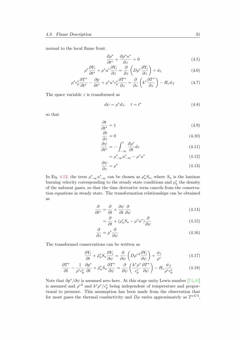
4.3. Flame Description 31
normal to the local flame front.
∂ρ∗
∂t∗+∂ρ∗u∗
∂z= 0 (4.5)
ρ∗∂Yi∂t∗
+ ρ∗u∗∂Yi∂z
=∂
∂z
(Dρ∗
∂Yi∂z
)+ wi (4.6)
ρ∗c∗p∂T ∗
∂t∗− ∂p
∂t∗+ ρ∗u∗c∗p
∂T ∗
∂z=
∂
∂z
(k∗∂T ∗
∂z
)−Hcwf (4.7)
The space variable z is transformed as
dψ = ρ∗dz, t = t∗ (4.8)
so that
∂t
∂t∗= 1 (4.9)
∂t
∂z= 0 (4.10)
∂ψ
∂t∗= −
∫ z
−∞
∂ρ∗
∂tdz (4.11)
= ρ∗−∞u∗−∞ − ρ∗u∗ (4.12)
∂ψ
∂z= ρ∗ (4.13)
In Eq. 4.12, the term ρ∗−∞u∗−∞ can be chosen as ρ∗uSu, where Su is the laminar
burning velocity corresponding to the steady state conditions and ρ∗u the densityof the unburnt gases, so that the time derivative term cancels from the conserva-tion equations in steady state. The transformation relationships can be obtainedas
∂
∂t∗=
∂
∂t+∂ψ
∂t
∂
∂ψ(4.14)
=∂
∂t+ (ρ∗uSu − ρ∗u∗)
∂
∂ψ(4.15)
∂
∂z= ρ∗
∂
∂ψ(4.16)
The transformed conservations can be written as
∂Yi∂t
+ ρ∗uSu∂Yi∂ψ
=∂
∂ψ
(Dρ∗2
∂Yi∂ψ
)+wiρ∗
(4.17)
∂T ∗
∂t− 1ρ∗c∗p
∂p∗
∂t+ ρ∗uSu
∂T ∗
∂ψ=
∂
∂ψ
(k∗ρ∗
c∗p
∂T ∗
∂ψ
)−Hc
wfρ∗c∗p
(4.18)
Note that ∂p∗/∂ψ is assumed zero here. At this stage unity Lewis number [74,41]is assumed and ρ∗2 and k∗ρ∗/c∗p being independent of temperature and propor-tional to pressure. This assumption has been made from the observation thatfor most gases the thermal conductivity and Dρ varies approximately as T ∗3/4,
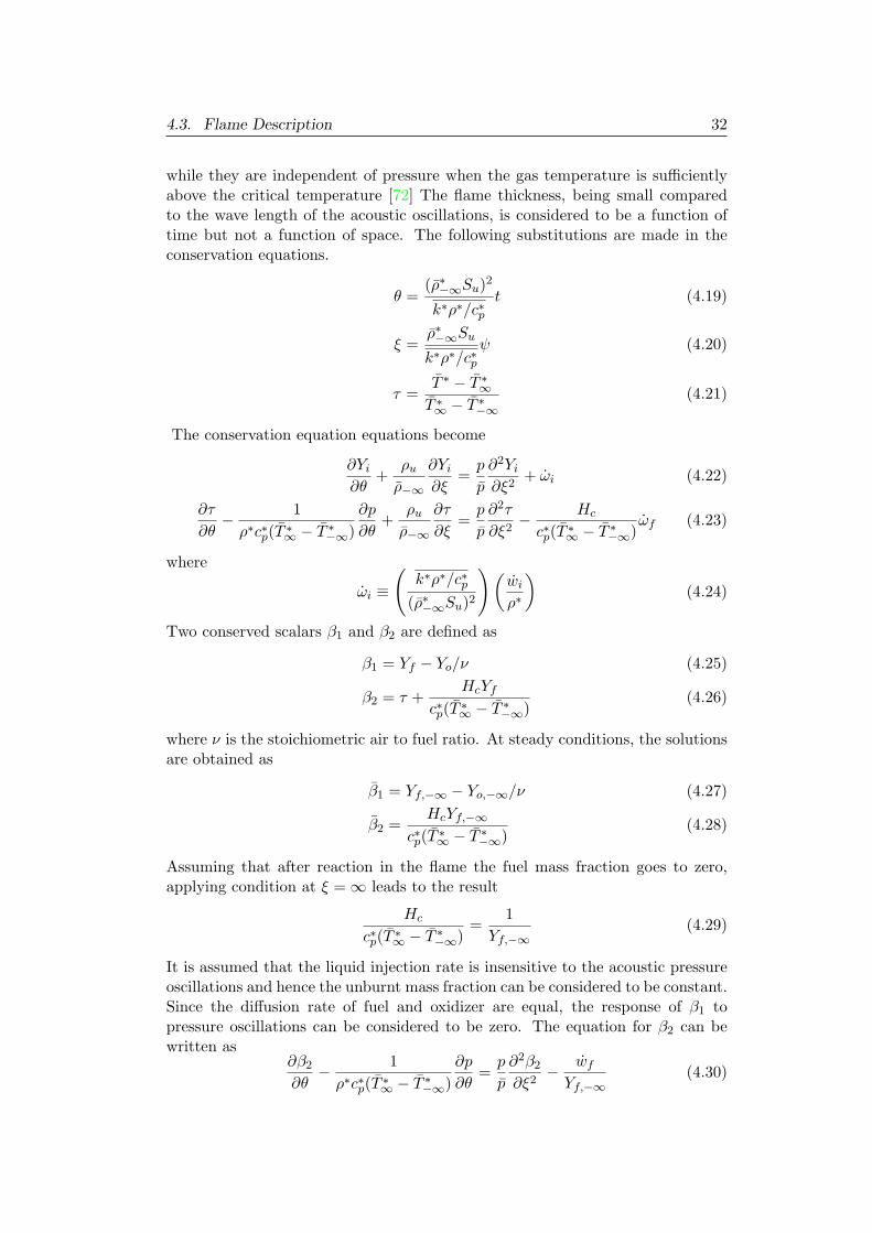
4.3. Flame Description 32
while they are independent of pressure when the gas temperature is sufficientlyabove the critical temperature [72] The flame thickness, being small comparedto the wave length of the acoustic oscillations, is considered to be a function oftime but not a function of space. The following substitutions are made in theconservation equations.
θ =(ρ∗−∞Su)2
k∗ρ∗/c∗pt (4.19)
ξ =ρ∗−∞Su
k∗ρ∗/c∗pψ (4.20)
τ =T ∗ − T ∗∞T ∗∞ − T ∗−∞
(4.21)
The conservation equation equations become
∂Yi∂θ
+ρuρ−∞
∂Yi∂ξ
=p
p
∂2Yi∂ξ2
+ ωi (4.22)
∂τ
∂θ− 1ρ∗c∗p(T ∗∞ − T ∗−∞)
∂p
∂θ+
ρuρ−∞
∂τ
∂ξ=p
p
∂2τ
∂ξ2− Hc
c∗p(T ∗∞ − T ∗−∞)ωf (4.23)
where
ωi ≡
(k∗ρ∗/c∗p
(ρ∗−∞Su)2
)(wiρ∗
)(4.24)
Two conserved scalars β1 and β2 are defined as
β1 = Yf − Yo/ν (4.25)
β2 = τ +HcYf
c∗p(T ∗∞ − T ∗−∞)(4.26)
where ν is the stoichiometric air to fuel ratio. At steady conditions, the solutionsare obtained as
β1 = Yf,−∞ − Yo,−∞/ν (4.27)
β2 =HcYf,−∞
c∗p(T ∗∞ − T ∗−∞)(4.28)
Assuming that after reaction in the flame the fuel mass fraction goes to zero,applying condition at ξ =∞ leads to the result
Hc
c∗p(T ∗∞ − T ∗−∞)=
1Yf,−∞
(4.29)
It is assumed that the liquid injection rate is insensitive to the acoustic pressureoscillations and hence the unburnt mass fraction can be considered to be constant.Since the diffusion rate of fuel and oxidizer are equal, the response of β1 topressure oscillations can be considered to be zero. The equation for β2 can bewritten as
∂β2
∂θ− 1ρ∗c∗p(T ∗∞ − T ∗−∞)
∂p
∂θ=p
p
∂2β2
∂ξ2−
wfYf,−∞
(4.30)
4.3. Flame Description 33
The second term of Eq. 4.30 can be shown to be equal to ∂β2,−∞/∂θ underthe assumption of spacially invariant pressure across the flame and isentropicconditions at the cold boundary. Hence Eq. 4.30 can be rewritten as
∂(β2 − β2,−∞)∂θ
+ρuρ−∞
∂(β2 − β2,−∞)∂ξ
=p
p
∂2(β2 − β2,−∞)∂ξ2
−wf
Yf,−∞(4.31)
The only solution to Eq. 4.31 which is finite at both ξ = ±∞ is β2 = β2,−∞These relations can now be utilized to represent all the dependent variables asfunction of a single dependent variable. τ is chosen as the dependent variable tobe solved. Hence
YfYf,−∞
= 1− (τ − τ−∞) (4.32)
YoYo,−∞
= 1− φ(τ − τ−∞) (4.33)
where φ is the equivalence ratio (≡ Yf,−∞ν/Yo,−∞). Hence the equation to besolved can be written as
∂(τ − τ−∞)∂θ
+ρuρ−∞
∂(τ − τ−∞)∂ξ =p
p
∂2(τ − τ−∞)∂ξ2
−ωf
Yf,−∞(4.34)
4.3.1 The reaction rate
The reaction rate is expressed as that of a second order single step reaction. Theform chosen is
wf = −AMfe−E/RT ∗T ∗cfco (4.35)
= − A
Moe−E/RT
∗ρ2T ∗YfYo (4.36)
= −(AM
MoR
)e−E/RT
∗p∗ρ∗YfYo (4.37)
The reaction rate can be expressed in terms of a single variable τ as
− ω
Yf,−∞=(k∗ρ∗/c∗p(ρuSu)2
)(AMYo,−∞p
MoR
)e−E/RT
∗∞1−β[(1−τ−∞)−(τ−τ−∞)]
×(p
p
)[1− (τ − τ−∞)][1− φ(τ − τ−∞)] (4.38)
where
β ≡T ∗∞ − T ∗−∞
T ∗∞(4.39)
4.3.2 Steady state solution
At steady state
τ−∞ = 0 (4.40)p
p= 1 (4.41)
4.3. Flame Description 34
and putting the time derivative to zero the conservation equation becomes
dτ
dξ=d2τ
dξ2+ λe−Θ/[1−β(1−τ)](1− τ)(1− φτ) (4.42)
where
λ ≡(k∗ρ∗/c∗p(ρuSu)2
)(AMYo,−∞p
MoR
)(4.43)
Θ ≡ E
RT ∗∞(4.44)
The steady state solution is obtained by the technique of matched asymptoticexpansion, with the assumption of large activation (i.e. large Θ). Under thisassumption an outer layer, where balance of conduction and convection takesplace and an inner layer where balance of reaction and conduction takes place.Substituting
χ ≡ dτ
dξ(4.45)
Eq. 4.42 becomes
χ− χdχdτ
= λe−Θ/[1−β(1−τ)](1− τ)(1− φτ) (4.46)
Under the assumption of large Θ, the order of magnitude of right hand side islower than any powers of 1/Θ and hence the outer solution is obtained as
χ = τ (4.47)
Since this solution is obviously not satisfactory uniformly everywhere in the do-main, an inner equation is obtained in the region τ → 1 A new variable η isdefined as
η ≡ Θ(1− τ) (4.48)
and Eq. 4.46 becomes
χ+ Θχdχ
dη= Λe−βη
η
Θ
[(1− φ)− φη
Θ
](4.49)
whereΛ ≡ λe−Θ (4.50)
An approximation of (1 − τ) is small has been made in deriving Eq. 4.49. Theanalysis varies slightly between the case when φ ∼ 1 and φ << 1.The classicalsolution using matched asymptotic expansion is reproduced here for the cases oflean mixture and for mixture close to stoichiometric conditions.
4.3. Flame Description 35
Analysis for φ << 1
When φ is not very close to unity, the following expansion can be made for thevariables in Eq. 4.49.
χ = χ0 +χ1
Θ+χ2
Θ2+ · · · (4.51)
Λ = Θ2
Λ0 +
Λ1
Θ+
Λ2
Θ2+ · · ·
(4.52)
and matching the coefficients of equal powers of Θ the following equations areobtained.
χ0dχ0
dη= (1− φ)Λ0ηe
−βη (4.53)
χ0 + χ0dχ1
dη+ χ1
dχ0
dη= (1− φ)Λ1ηe
−βη − φΛ0η2e−βη (4.54)
...
Integration of Eq. 4.53 and applying the boundary condition at η = 0 (τ = 1 orξ →∞)
χ20
2=
(1− φ)Λ0
β21− (1 + βη)e−βη (4.55)
Matching the inner and the outer solutions using Kaplun’s matching theorem [75],which states (
Inner limit ofthe outer solution
)=(
Outer limit ofthe inner solution
)(4.56)
we get(1− φ)Λ0
β2=
12
(4.57)
The solution, which is uniformly valid for the entire region is obtained as
χ = τ + 1− [1 + βΘ(1− τ)]e−βΘ(1−τ)1/2 − 1 (4.58)
The burning rate can be obtained by substituting the variables of Eq. 4.57 as
(ρuSu)2 = 2(
1− φβ2
)(k∗ρ∗
c∗p
)(AMYo,−∞p
MoR
)e−E/RT∞
(E/RT∞)2(4.59)
Analysis for φ ∼ 1
When φ ∼ 1, we define α ≡ Θ(1 − φ) which is O(1). Hence Eq. 4.49 can bewritten as
χ+ Θχdχ
dη= Λe−βη
η
Θ2[α− φη] (4.60)
The expansion for Λ is changed slightly to
χ = χ0 +χ1
Θ+χ2
Θ2+ · · · (4.61)
Λ = Θ3
Λ0 +
Λ1
Θ+
Λ2
Θ2+ · · ·
(4.62)
4.4. Unsteady Response 36
in order to match the terms. Matching the coefficients of equal powers of Θ gives
χ0dχ0
dη= Λ0e
−βηη(α− φη) (4.63)
χ0 + χ0dχ1
dη+ χ1
dχ0
dη= Λ1e
−βηη(α− φη) (4.64)
...
The solution of Eq. 4.63 with the boundary condition applied at τ = 1 is
χ20
2= Λ0
2φ+ αβ
β3
1−
(β2φ
2φ+ αβη2 + βη + 1
)eβη
(4.65)
and application of matching condition gives
Λ02φ+ αβ
β3=
12
(4.66)
The solution uniformly valid is
χ = τ − 1+1−
(φ
2φ+ Θβ(1− φ)Θ2β2(1− τ)2 + Θβ(1− τ) + 1
)e−Θβ(1−τ)
1/2
(4.67)
The burning rate is obtained as
(ρuSu)2 = 2(
(2φ+ Θβ(1− φ)Θ3β3
)(k∗ρ∗
c∗p
)(AMYo,−∞p
MoR
)e−E/RT−∞ (4.68)
4.4 Unsteady Response
The following substitutions are made into Eq. 4.34
τg ≡ τ − τ−∞ (4.69)p
p= 1 + p′ (4.70)
and obtain
∂τg∂θ
+∂τg∂ξ
= (1 + p′)∂2τg∂ξ2
+ λe−Θ/1−β(1−τg)+βτ−∞(1 + p′)(1− τg)(1− φτg) (4.71)
The linearized response equation can be derived from this as
∂τ ′g∂θ
+∂τ ′g∂ξ
=∂2τ ′g∂ξ2
+ p′∂2τ
∂ξ2+ ω′ (4.72)
where
ω′ = ¯ω
Θβ[1− β(1− τ)]2
(τ−∞ − τ ′g) + p′ −(
11− τ
+φ
1− φτ
)τ ′g
(4.73)
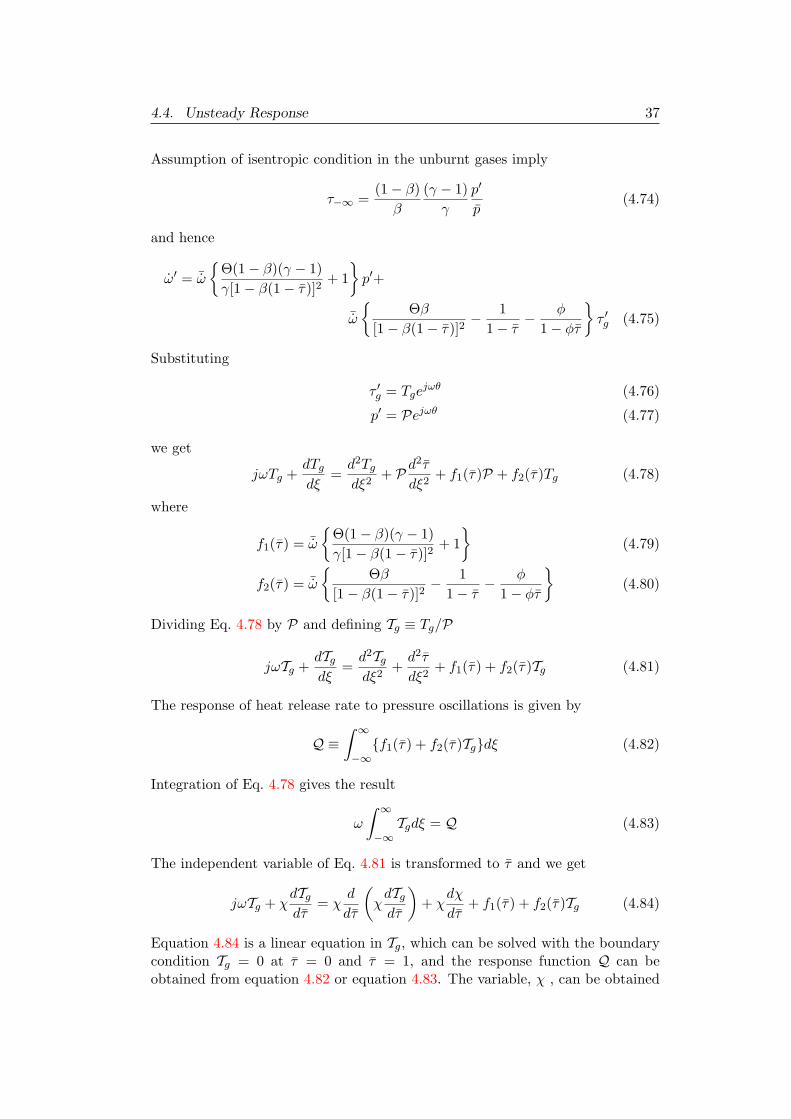
4.4. Unsteady Response 37
Assumption of isentropic condition in the unburnt gases imply
τ−∞ =(1− β)β
(γ − 1)γ
p′
p(4.74)
and hence
ω′ = ¯ω
Θ(1− β)(γ − 1)γ[1− β(1− τ)]2
+ 1p′+
¯ω
Θβ[1− β(1− τ)]2
− 11− τ
− φ
1− φτ
τ ′g (4.75)
Substituting
τ ′g = Tgejωθ (4.76)
p′ = Pejωθ (4.77)
we get
jωTg +dTgdξ
=d2Tgdξ2
+ P d2τ
dξ2+ f1(τ)P + f2(τ)Tg (4.78)
where
f1(τ) = ¯ω
Θ(1− β)(γ − 1)γ[1− β(1− τ)]2
+ 1
(4.79)
f2(τ) = ¯ω
Θβ[1− β(1− τ)]2
− 11− τ
− φ
1− φτ
(4.80)
Dividing Eq. 4.78 by P and defining Tg ≡ Tg/P
jωTg +dTgdξ
=d2Tgdξ2
+d2τ
dξ2+ f1(τ) + f2(τ)Tg (4.81)
The response of heat release rate to pressure oscillations is given by
Q ≡∫ ∞−∞f1(τ) + f2(τ)Tgdξ (4.82)
Integration of Eq. 4.78 gives the result
ω
∫ ∞−∞Tgdξ = Q (4.83)
The independent variable of Eq. 4.81 is transformed to τ and we get
jωTg + χdTgdτ
= χd
dτ
(χdTgdτ
)+ χ
dχ
dτ+ f1(τ) + f2(τ)Tg (4.84)
Equation 4.84 is a linear equation in Tg, which can be solved with the boundarycondition Tg = 0 at τ = 0 and τ = 1, and the response function Q can beobtained from equation 4.82 or equation 4.83. The variable, χ , can be obtained
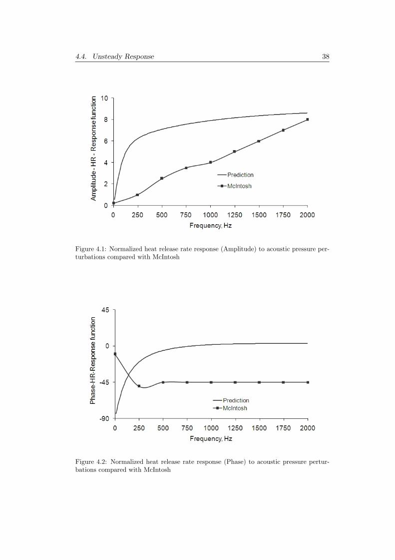
4.4. Unsteady Response 38
Figure 4.1: Normalized heat release rate response (Amplitude) to acoustic pressure per-turbations compared with McIntosh
Figure 4.2: Normalized heat release rate response (Phase) to acoustic pressure pertur-bations compared with McIntosh
4.5. Solution Procedure and software implementation 39
from equation 4.58 or equation 4.67 depending on the range of equivalence ratio.Only numerical integration is attempted in the present case.
Figures 4.1 and 4.2, show the amplitude and phase of heat release response toacoustic fluctuations for a frequency range of 0 to 2000 Hz. The results obtainedby McIntosh [41] is also included for comparison. As can be seen, the real part ofthe response function increases to a constant value as and the phase increases from−90 to a positive maximum and decreases to zero. This behaviour is inbuilt inthe one dimensional flame description. The reaction rate considered is of secondorder, which implies that the rate increases as the square of pressure. However asthe reaction rate increases there will be a corresponding reduction in the reactantconcentration, which in turn reduces the reaction rate. The response of reactantconcentration is slower compared to the response of the reaction rate itself becausesome time is required for the concentration to come down to the equilibrium (orquasi-steady) values. Hence at high frequencies the reaction rate responds to thechanges in pressure without any phase lag. However, the results of McIntoshseem to show unrestricted increase in the amplitude ratio as frequency increases.As indicated in Section 4.1 the dependence of concentration and temperaturefluctuations within the reaction zone was not accounted in Ref. [41] and hencethe unrestricted linear growth of FRF, which is not physically realistic.
In the above analysis the effects due to the changes in mixture ratio, the flamesurface density and the surface area of the flame brush have been neglected. Theearlier authors have considered these in their analysis, while neglecting the effectsof flame response itself. The primary consideration has been the flame surfacearea variation. Much of these effects are likely to be present at low frequenciesand low equivalence ratios. Since screech analysis in afterburners, with which weare concerned in this thesis, corresponds to equivalence ratio close to one andrelatively high frequencies, the current model proposed is expected to be moreappropriate than the older combustion response models.
Unlike the response to the velocity fluctuations, the response function due topressure fluctuations increase with frequency as shown in Fig. 4.1. The magni-tude of response function due to pressure fluctuations is much larger than thatdue to velocity fluctuations even at frequencies as low as l00 Hz.
4.5 Solution Procedure and software implementation
Refer to section 3.2 for general solution procedure. In this section the imple-mentation of user defined combustion source response function in SYSNOISE ispresented.
In the experiments, though within the pre-heater non-uniform temperaturedistribution exists, the same is properly nullified by its construction itself, by thetime the vitiated products reach the entrance of the afterburner. This aspect isclosely examined in the testing by having a temperature rake at the entry to af-terburner with six points, as the temperature determines its acoustic propagationspeed and in turn the characteristic impedance of a fluid. Thus uniform temper-ature profile is made available within the test section. Based on the temperatureand on the mean pre heater pressure, acoustic speed and fluid density, the ma-
4.5. Solution Procedure and software implementation 40
terial is defined for the entire acoustic domain. The complex convergent nozzleadmittance which is computed separately for the choked condition is applied atthe entry to the nozzle. In the first run the acoustic pressure distribution in theentire region of acoustic mesh is calculated.
Further, the acoustics in the afterburner are forced by the unsteady heat re-lease rate. To this effect, the gain from the unsteady heat release rate to panelvibration velocity is obtained by the equations given in section 4.2. The combus-tion response function which is obtained by solving equation 4.82 is imposed inthe flame stabilizer region of acoustic mesh.
The coupled combustion oscillations—amplitude and phase—due to reheatoperation were estimated by superimposing heat release fluctuations on the acous-tic pressure history obtained by solving the homogeneous wave equation (referFig 3.2). Figure 4.3 shows coupled normalized acoustic pressure amplitude andphase spectrum.
Then, admittance—that pertains to screech liner—boundary condition throughtransfer relation is imposed on the inner and outer perforate which connects thecore and bypass passages of the afterburner. The results are discussed in Chapter6.
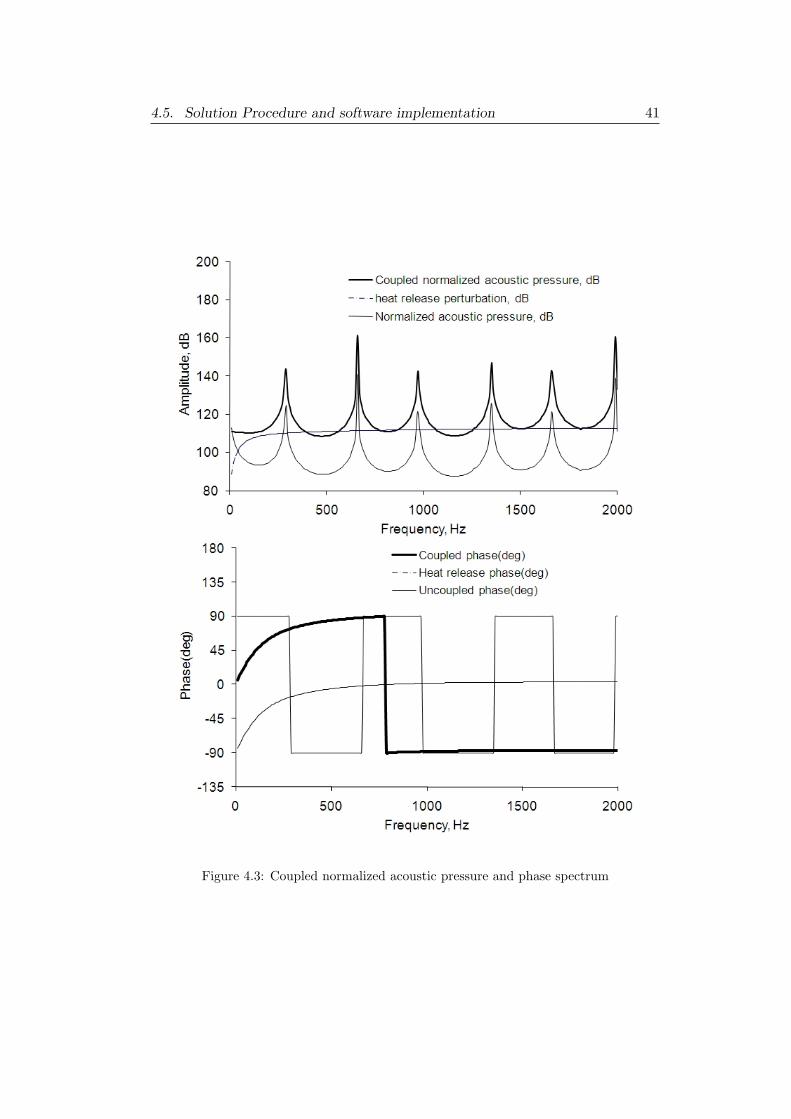
4.5. Solution Procedure and software implementation 41
Figure 4.3: Coupled normalized acoustic pressure and phase spectrum
Chapter 5
Experiments
The actual configuration of afterburner was tested to study the complete be-haviour of afterburner with respect to the phenomenon of combustion instability.These tests were also for confirmation of theoretically predicted screech frequen-cies. The test programs practical implication is that when the instability occurs,the amplitudes of oscillations at various frequencies do not overshoot the per-missible limits for the safe afterburner operation with the provision of perforatedliner.
In the experiments the duct modes (longitudinal) are excited due to incomingaerodynamic disturbances from the slave combustor, and tangential modes aretriggered during afterburner operation. In theoretical analysis, the type of inletcondition that existed in the experiments was not imposed whereas the pressurewave-flame interaction source model which characterizes combustion instabilityphenomenon in the region of afterburner is considered. As the inlet conditionsin the theoretical analysis and the experiments are not the same and since thenon-linear effects are not considered in the theoretical analysis, the amplitudesof acoustic oscillations that are observed in the experiments are not directlycomparable. However, the frequency spectrum is comparable in predictions andexperiments. Thus, while bringing out several aspects of combustion instabilityfrom experiments, the predicted modes (frequencies- longitudinal and tangential)are compared with experimental results, to validate theoretical development.
In this chapter, the experimental work carried out is described. First, after-burner test facility description and its capabilities are given. Then, test sectionpreparation along with dynamic pressure probes is given. Finally, the conduc-tion of experiments is presented along with some sample data that was processedthrough FFT analyser.
5.1 Afterburner test facility
To simulate Afterburner entry conditions, afterburner test facility is employed.The process and instrumentation diagram is shown in figure 5.1. The test facilitycapabilities are enumerated in Table 5.1. The air is drawn from High mass flowhigh pressure air supply facility (HMFHPASF) which is located about 50 metersfrom the Afterburner test facility.
42
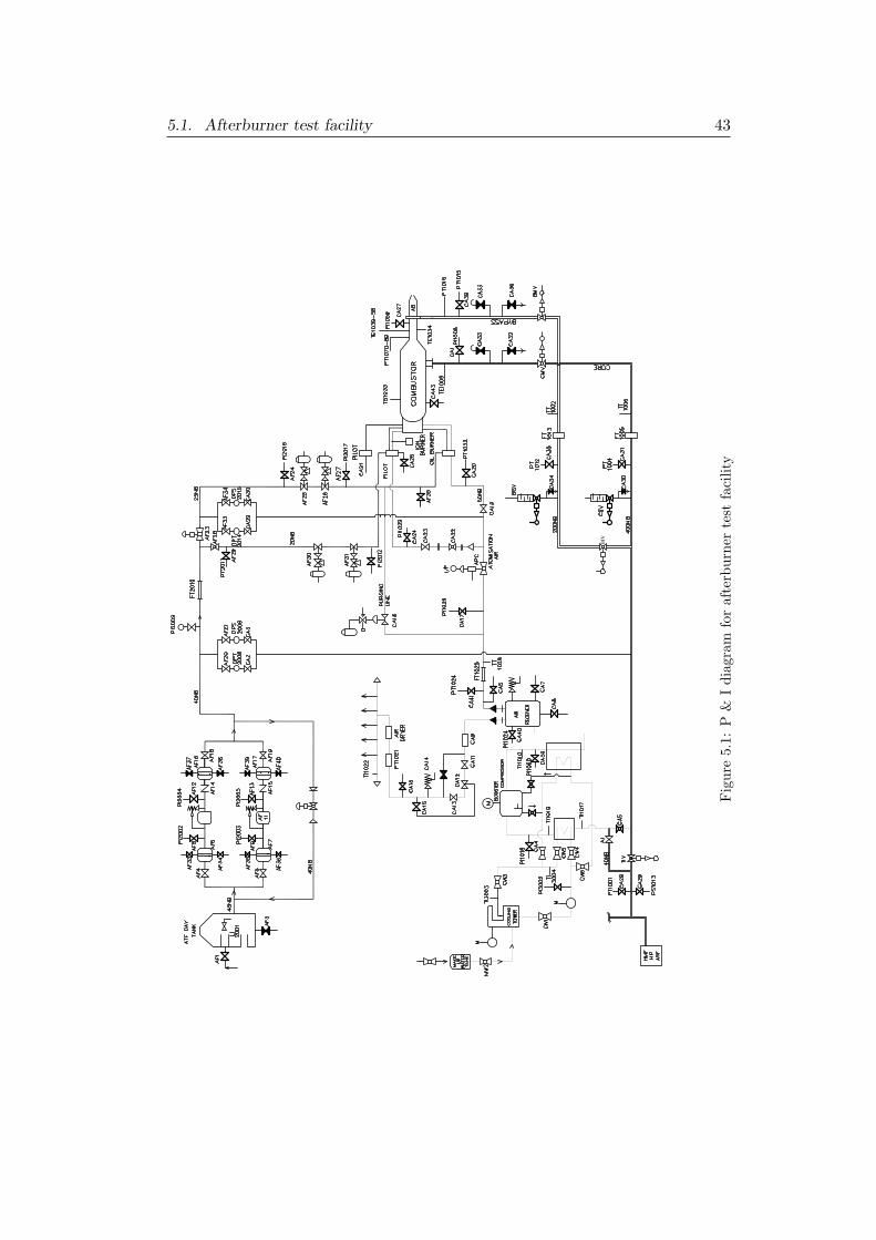
5.1. Afterburner test facility 43
Fig
ure
5.1:
P&
Idi
agra
mfo
raf
terb
urne
rte
stfa
cilit
y
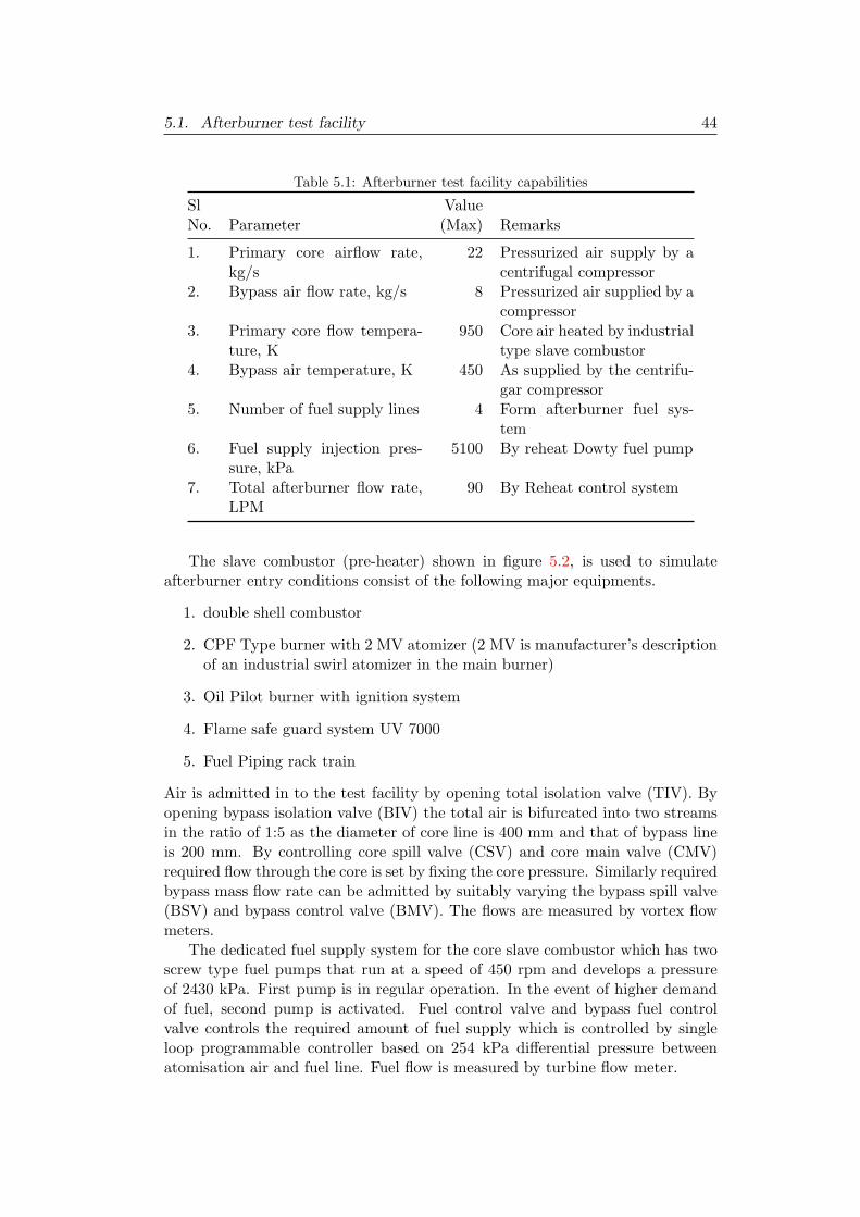
5.1. Afterburner test facility 44
Table 5.1: Afterburner test facility capabilities
Sl ValueNo. Parameter (Max) Remarks
1. Primary core airflow rate,kg/s
22 Pressurized air supply by acentrifugal compressor
2. Bypass air flow rate, kg/s 8 Pressurized air supplied by acompressor
3. Primary core flow tempera-ture, K
950 Core air heated by industrialtype slave combustor
4. Bypass air temperature, K 450 As supplied by the centrifu-gar compressor
5. Number of fuel supply lines 4 Form afterburner fuel sys-tem
6. Fuel supply injection pres-sure, kPa
5100 By reheat Dowty fuel pump
7. Total afterburner flow rate,LPM
90 By Reheat control system
The slave combustor (pre-heater) shown in figure 5.2, is used to simulateafterburner entry conditions consist of the following major equipments.
1. double shell combustor
2. CPF Type burner with 2 MV atomizer (2 MV is manufacturer’s descriptionof an industrial swirl atomizer in the main burner)
3. Oil Pilot burner with ignition system
4. Flame safe guard system UV 7000
5. Fuel Piping rack train
Air is admitted in to the test facility by opening total isolation valve (TIV). Byopening bypass isolation valve (BIV) the total air is bifurcated into two streamsin the ratio of 1:5 as the diameter of core line is 400 mm and that of bypass lineis 200 mm. By controlling core spill valve (CSV) and core main valve (CMV)required flow through the core is set by fixing the core pressure. Similarly requiredbypass mass flow rate can be admitted by suitably varying the bypass spill valve(BSV) and bypass control valve (BMV). The flows are measured by vortex flowmeters.
The dedicated fuel supply system for the core slave combustor which has twoscrew type fuel pumps that run at a speed of 450 rpm and develops a pressureof 2430 kPa. First pump is in regular operation. In the event of higher demandof fuel, second pump is activated. Fuel control valve and bypass fuel controlvalve controls the required amount of fuel supply which is controlled by singleloop programmable controller based on 254 kPa differential pressure betweenatomisation air and fuel line. Fuel flow is measured by turbine flow meter.
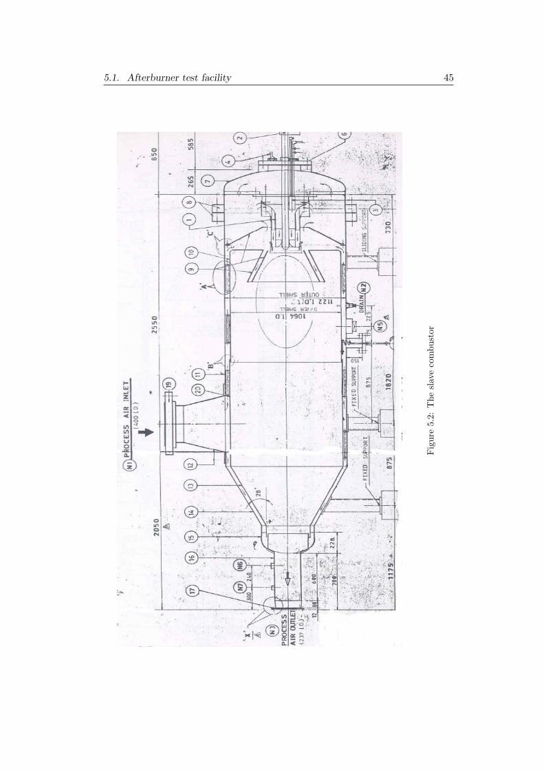
5.1. Afterburner test facility 45
Fig
ure
5.2:
The
slav
eco
mbu
stor
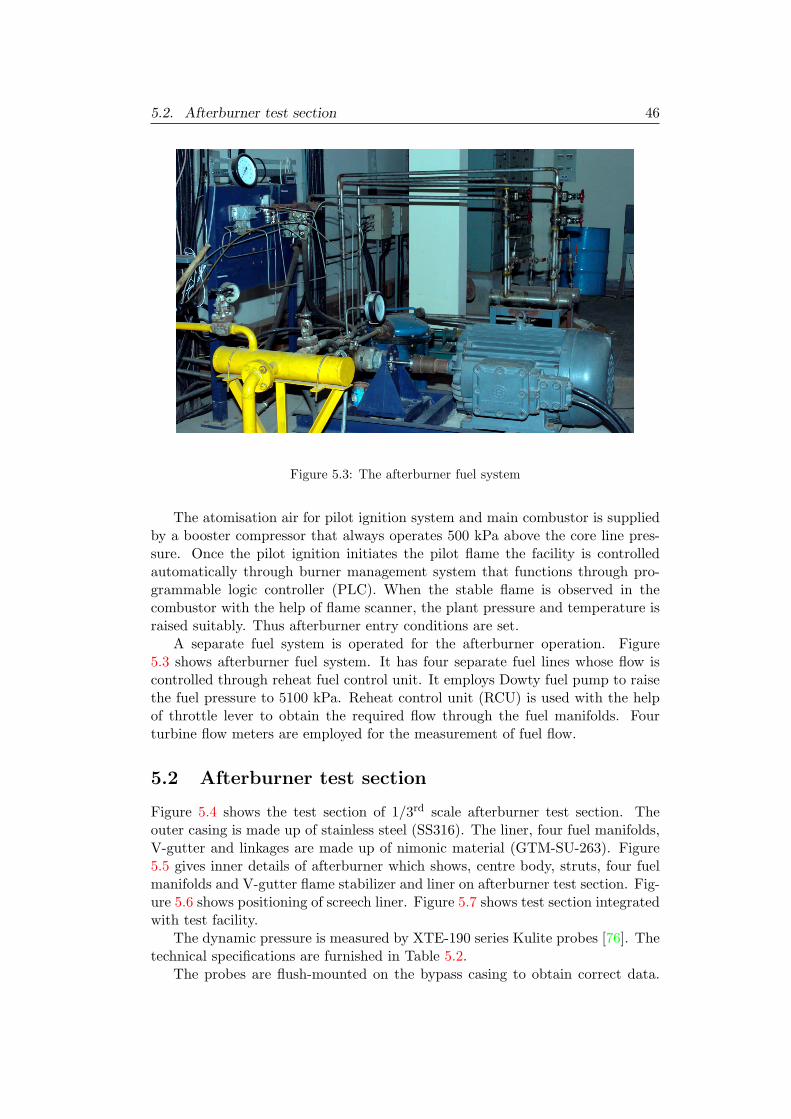
5.2. Afterburner test section 46
Figure 5.3: The afterburner fuel system
The atomisation air for pilot ignition system and main combustor is suppliedby a booster compressor that always operates 500 kPa above the core line pres-sure. Once the pilot ignition initiates the pilot flame the facility is controlledautomatically through burner management system that functions through pro-grammable logic controller (PLC). When the stable flame is observed in thecombustor with the help of flame scanner, the plant pressure and temperature israised suitably. Thus afterburner entry conditions are set.
A separate fuel system is operated for the afterburner operation. Figure5.3 shows afterburner fuel system. It has four separate fuel lines whose flow iscontrolled through reheat fuel control unit. It employs Dowty fuel pump to raisethe fuel pressure to 5100 kPa. Reheat control unit (RCU) is used with the helpof throttle lever to obtain the required flow through the fuel manifolds. Fourturbine flow meters are employed for the measurement of fuel flow.
5.2 Afterburner test section
Figure 5.4 shows the test section of 1/3rd scale afterburner test section. Theouter casing is made up of stainless steel (SS316). The liner, four fuel manifolds,V-gutter and linkages are made up of nimonic material (GTM-SU-263). Figure5.5 gives inner details of afterburner which shows, centre body, struts, four fuelmanifolds and V-gutter flame stabilizer and liner on afterburner test section. Fig-ure 5.6 shows positioning of screech liner. Figure 5.7 shows test section integratedwith test facility.
The dynamic pressure is measured by XTE-190 series Kulite probes [76]. Thetechnical specifications are furnished in Table 5.2.
The probes are flush-mounted on the bypass casing to obtain correct data.
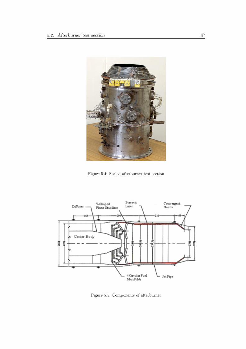
5.2. Afterburner test section 47
Figure 5.4: Scaled afterburner test section
Figure 5.5: Components of afterburner
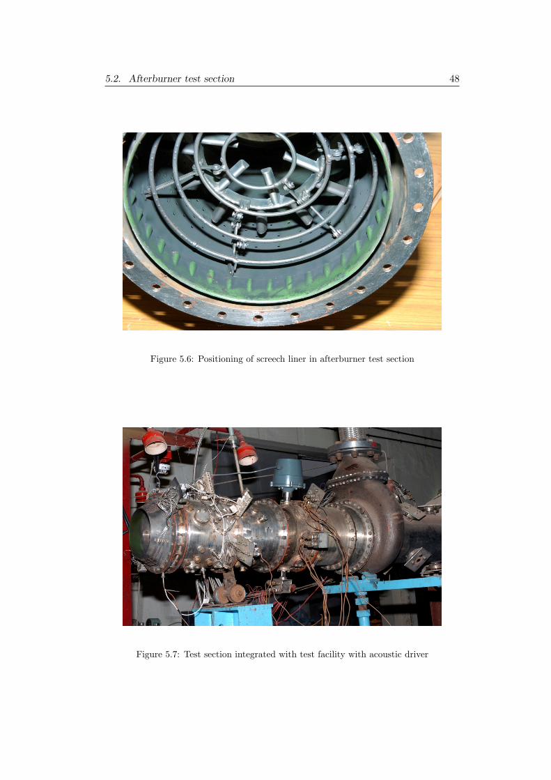
5.2. Afterburner test section 48
Figure 5.6: Positioning of screech liner in afterburner test section
Figure 5.7: Test section integrated with test facility with acoustic driver
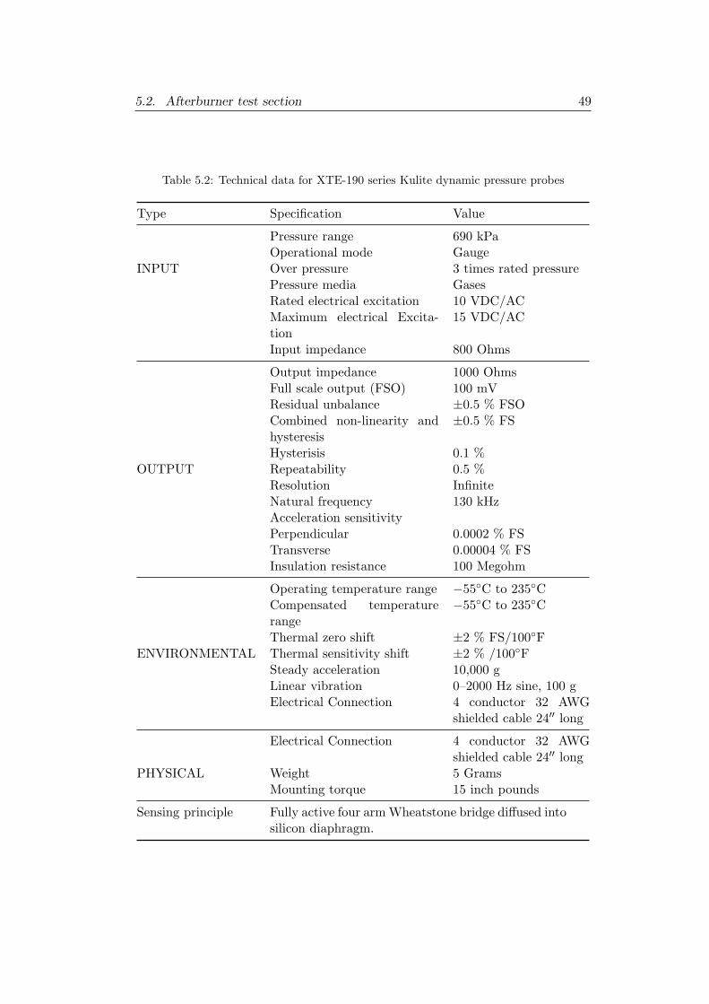
5.2. Afterburner test section 49
Table 5.2: Technical data for XTE-190 series Kulite dynamic pressure probes
Type Specification Value
Pressure range 690 kPaOperational mode Gauge
INPUT Over pressure 3 times rated pressurePressure media GasesRated electrical excitation 10 VDC/ACMaximum electrical Excita-tion
15 VDC/AC
Input impedance 800 Ohms
Output impedance 1000 OhmsFull scale output (FSO) 100 mVResidual unbalance ±0.5 % FSOCombined non-linearity andhysteresis
±0.5 % FS
Hysterisis 0.1 %OUTPUT Repeatability 0.5 %
Resolution InfiniteNatural frequency 130 kHzAcceleration sensitivityPerpendicular 0.0002 % FSTransverse 0.00004 % FSInsulation resistance 100 Megohm
Operating temperature range −55C to 235CCompensated temperaturerange
−55C to 235C
Thermal zero shift ±2 % FS/100FENVIRONMENTAL Thermal sensitivity shift ±2 % /100F
Steady acceleration 10,000 gLinear vibration 0–2000 Hz sine, 100 gElectrical Connection 4 conductor 32 AWG
shielded cable 24′′ long
Electrical Connection 4 conductor 32 AWGshielded cable 24′′ long
PHYSICAL Weight 5 GramsMounting torque 15 inch pounds
Sensing principle Fully active four arm Wheatstone bridge diffused intosilicon diaphragm.
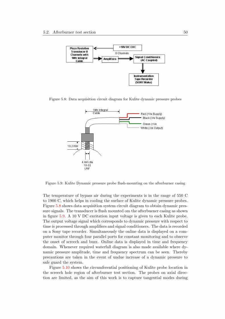
5.2. Afterburner test section 50
Figure 5.8: Data acquisition circuit diagram for Kulite dynamic pressure probes
Figure 5.9: Kulite Dynamic pressure probe flush-mounting on the afterburner casing
The temperature of bypass air during the experiments is in the range of 550 Cto 1900 C, which helps in cooling the surface of Kulite dynamic pressure probes.Figure 5.8 shows data acquisition system circuit diagram to obtain dynamic pres-sure signals. The transducer is flush mounted om the afterbuener casing as shownin figure 5.9. A 10 V DC excitation input voltage is given to each Kulite probe.The output voltage signal which corresponds to dynamic pressure with respect totime is processed through amplifiers and signal conditioners. The data is recordedon a Sony tape recorder. Simultaneously the online data is displayed on a com-puter monitor through four parallel ports for constant monitoring and to observethe onset of screech and buzz. Online data is displayed in time and frequencydomain. Whenever required waterfall diagram is also made available where dy-namic pressure amplitude, time and frequency spectrum can be seen. Therebyprecautions are taken in the event of undue increase of a dynamic pressure tosafe guard the system.
Figure 5.10 shows the circumferential positioning of Kulite probe location inthe screech hole region of afterburner test section. The probes on axial direc-tion are limited, as the aim of this work is to capture tangential modes during
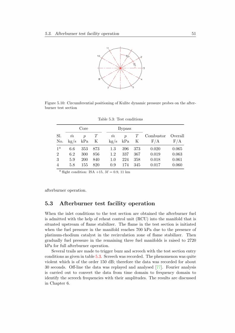
5.3. Afterburner test facility operation 51
Figure 5.10: Circumferential positioning of Kulite dynamic pressure probes on the after-burner test section
Table 5.3: Test conditions
Core Bypass
Sl. m p T m p T Combustor OverallNo. kg/s kPa K kg/s kPa K F/A F/A
1a 6.6 353 873 1.3 396 373 0.020 0.0652 6.2 300 856 1.2 337 367 0.019 0.0633 5.9 200 840 1.0 224 358 0.018 0.0614 5.8 155 820 0.9 174 345 0.017 0.060a flight condition: ISA +15, M = 0.9, 11 km
afterburner operation.
5.3 Afterburner test facility operation
When the inlet conditions to the test section are obtained the afterburner fuelis admitted with the help of reheat control unit (RCU) into the manifold that issituated upstream of flame stabilizer. The flame in the test section is initiatedwhen the fuel pressure in the manifold reaches 700 kPa due to the presence ofplatinum-rhodium catalyst in the recirculation zone of flame stabilizer. Thengradually fuel pressure in the remaining three fuel manifolds is raised to 2720kPa for full afterburner operation.
Several trails are made to trigger buzz and screech with the test section entryconditions as given in table 5.3. Screech was recorded. The phenomenon was quiteviolent which is of the order 150 dB; therefore the data was recorded for about30 seconds. Off-line the data was replayed and analysed [77]. Fourier analysisis carried out to convert the data from time domain to frequency domain toidentify the screech frequencies with their amplitudes. The results are discussedin Chapter 6.
Chapter 6
Results and Discussion
The results of both the experiments and the computations are presented anddiscussed in this chapter. The results are discussed under the following sub-headings.
1. Frequency characterization of test section
2. Identification of pure and coupled screech modes by analysis
3. Study of effectiveness of screech liner by variation in porosity
4. Attenuation characteristics with 2.5 % porosity liner
5. Comparison of theoretical and experimental results.
6.1 Frequency characterization of test section
Figure 6.1 shows the Afterburner test section that was used to conduct testsin the Afterburner test facility. Test results that are presented in this chaptercorrespond to the test conditions shown in the table 6.1. During testing core,bypass conditions, combustor fuel to air ratio and overall fuel air ratio (Combustorand afterburner) are simulated.
Figure 6.2 shows the afterburner configuration that was modelled for FEMacoustic analysis. The acoustic mesh is modelled from the slave combustor exitonwards. Centre body, symmetrical struts and flame stabiliser are taken intoaccount in meshing. Bypass air column is provided where the perforate liner ispositioned. The software limits the use of different core and bypass conditions,by which it means fluid properties for bypass acoustic medium are same as thatof core. Hence for core and bypass, conditions as shown in table 6.1 are used foranalysis.
The frequency spectrum for the afterburner for a range from 10 Hz to 2000Hz is predicted. The normalized acoustic pressure in dB and corresponding phasein degrees are plotted in the figure 6.3. The analysis is carried out with an inletexcitation particle velocity of 1 + 0j m/s. This value was chosen to be consistentwith several earlier researchers in the field [78, 27]. Hence, this magnitude willresult in the prediction of acoustic pressure in the range of 150 dB to 220 dB.
52
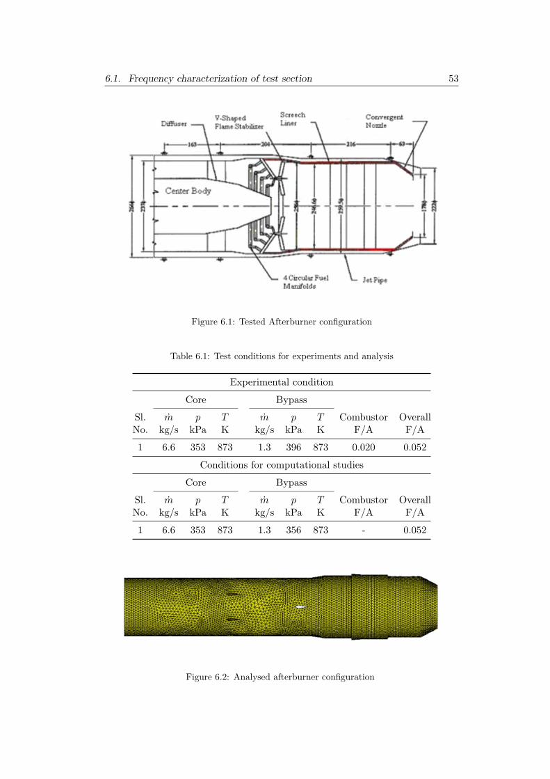
6.1. Frequency characterization of test section 53
Figure 6.1: Tested Afterburner configuration
Table 6.1: Test conditions for experiments and analysis
Experimental condition
Core Bypass
Sl. m p T m p T Combustor OverallNo. kg/s kPa K kg/s kPa K F/A F/A
1 6.6 353 873 1.3 396 873 0.020 0.052
Conditions for computational studies
Core Bypass
Sl. m p T m p T Combustor OverallNo. kg/s kPa K kg/s kPa K F/A F/A
1 6.6 353 873 1.3 356 873 - 0.052
Figure 6.2: Analysed afterburner configuration
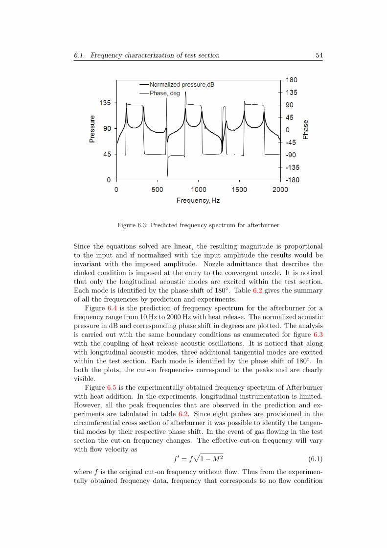
6.1. Frequency characterization of test section 54
Figure 6.3: Predicted frequency spectrum for afterburner
Since the equations solved are linear, the resulting magnitude is proportionalto the input and if normalized with the input amplitude the results would beinvariant with the imposed amplitude. Nozzle admittance that describes thechoked condition is imposed at the entry to the convergent nozzle. It is noticedthat only the longitudinal acoustic modes are excited within the test section.Each mode is identified by the phase shift of 180. Table 6.2 gives the summaryof all the frequencies by prediction and experiments.
Figure 6.4 is the prediction of frequency spectrum for the afterburner for afrequency range from 10 Hz to 2000 Hz with heat release. The normalized acousticpressure in dB and corresponding phase shift in degrees are plotted. The analysisis carried out with the same boundary conditions as enumerated for figure 6.3with the coupling of heat release acoustic oscillations. It is noticed that alongwith longitudinal acoustic modes, three additional tangential modes are excitedwithin the test section. Each mode is identified by the phase shift of 180. Inboth the plots, the cut-on frequencies correspond to the peaks and are clearlyvisible.
Figure 6.5 is the experimentally obtained frequency spectrum of Afterburnerwith heat addition. In the experiments, longitudinal instrumentation is limited.However, all the peak frequencies that are observed in the prediction and ex-periments are tabulated in table 6.2. Since eight probes are provisioned in thecircumferential cross section of afterburner it was possible to identify the tangen-tial modes by their respective phase shift. In the event of gas flowing in the testsection the cut-on frequency changes. The effective cut-on frequency will varywith flow velocity as
f ′ = f√
1−M2 (6.1)
where f is the original cut-on frequency without flow. Thus from the experimen-tally obtained frequency data, frequency that corresponds to no flow condition
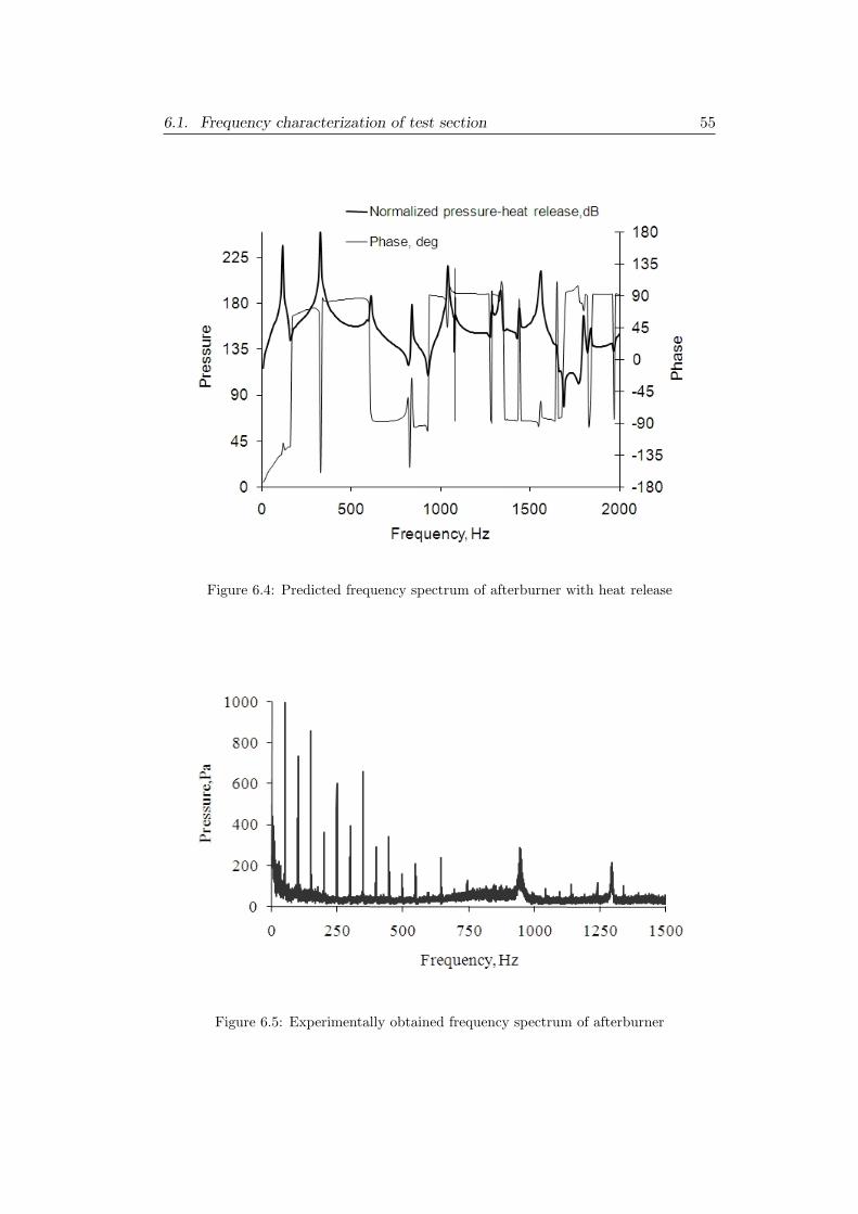
6.1. Frequency characterization of test section 55
Figure 6.4: Predicted frequency spectrum of afterburner with heat release
Figure 6.5: Experimentally obtained frequency spectrum of afterburner
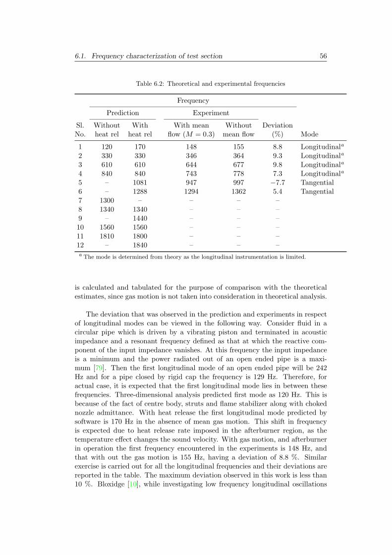
6.1. Frequency characterization of test section 56
Table 6.2: Theoretical and experimental frequencies
Frequency
Prediction Experiment
Sl. Without With With mean Without DeviationNo. heat rel heat rel flow (M = 0.3) mean flow (%) Mode
1 120 170 148 155 8.8 Longitudinala
2 330 330 346 364 9.3 Longitudinala
3 610 610 644 677 9.8 Longitudinala
4 840 840 743 778 7.3 Longitudinala
5 – 1081 947 997 −7.7 Tangential6 – 1288 1294 1362 5.4 Tangential7 1300 – – – –8 1340 1340 – – –9 – 1440 – – –10 1560 1560 – – –11 1810 1800 – – –12 – 1840 – – –a The mode is determined from theory as the longitudinal instrumentation is limited.
is calculated and tabulated for the purpose of comparison with the theoreticalestimates, since gas motion is not taken into consideration in theoretical analysis.
The deviation that was observed in the prediction and experiments in respectof longitudinal modes can be viewed in the following way. Consider fluid in acircular pipe which is driven by a vibrating piston and terminated in acousticimpedance and a resonant frequency defined as that at which the reactive com-ponent of the input impedance vanishes. At this frequency the input impedanceis a minimum and the power radiated out of an open ended pipe is a maxi-mum [79]. Then the first longitudinal mode of an open ended pipe will be 242Hz and for a pipe closed by rigid cap the frequency is 129 Hz. Therefore, foractual case, it is expected that the first longitudinal mode lies in between thesefrequencies. Three-dimensional analysis predicted first mode as 120 Hz. This isbecause of the fact of centre body, struts and flame stabilizer along with chokednozzle admittance. With heat release the first longitudinal mode predicted bysoftware is 170 Hz in the absence of mean gas motion. This shift in frequencyis expected due to heat release rate imposed in the afterburner region, as thetemperature effect changes the sound velocity. With gas motion, and afterburnerin operation the first frequency encountered in the experiments is 148 Hz, andthat with out the gas motion is 155 Hz, having a deviation of 8.8 %. Similarexercise is carried out for all the longitudinal frequencies and their deviations arereported in the table. The maximum deviation observed in this work is less than10 %. Bloxidge [10], while investigating low frequency longitudinal oscillations
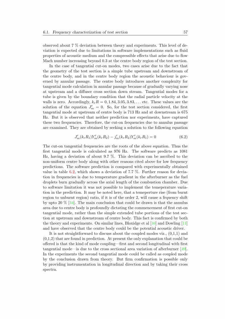
6.1. Frequency characterization of test section 57
observed about 7 % deviation between theory and experiments. This level of de-viation is expected due to limitations in software implementations such as fluidproperties of acoustic medium and the compressible effects that arise due to flowMach number increasing beyond 0.3 at the centre body region of the test section.
In the case of tangential cut-on modes, two cases arise due to the fact thatthe geometry of the test section is a simple tube upstream and downstream ofthe centre body, and in the centre body region the acoustic behaviour is gov-erned by annular passage. The centre body introduces another complexity fortangential mode calculation in annular passage because of gradually varying noseat upstream and a diffuser cross section down stream. Tangential modes for atube is given by the boundary condition that the radial particle velocity at thewalls is zero. Accordingly, krR = 0, 1.84, 3.05, 3.83, . . . etc. These values are thesolution of the equation J ′m = 0. So, for the test section considered, the firsttangential mode at upstream of centre body is 713 Hz and at downstream is 675Hz. But it is observed that neither prediction nor experiments, have capturedthese two frequencies. Therefore, the cut-on frequencies due to annulus passageare examined. They are obtained by seeking a solution to the following equation
J ′m(krR1)Y ′m(krR2)− j′m(krR2)Y ′m(krR1) = 0 (6.2)
The cut-on tangential frequencies are the roots of the above equation. Thus thefirst tangential mode is calculated as 976 Hz. The software predicts as 1081Hz, having a deviation of about 9.7 %. This deviation can be ascribed to thenon-uniform centre body along with other reasons cited above for low frequencypredictions. The software prediction is compared with experimentally obtainedvalue in table 6.2, which shows a deviation of 7.7 %. Further reason for devia-tion in frequencies is due to temperature gradient in the afterburner as the fueldroplets burn gradually across the axial length of the combustion chamber. Dueto software limitation it was not possible to implement the temeperature varia-tion in the prediction. It may be noted here, that a temeperture rise (from burntregion to unburnt region) ratio, if it is of the order 2, will cause a frquency shiftby upto 20 % [34]. The main conclusion that could be drawn is that the annulusarea due to centre body is profoundly dictating the commencement of first cut-ontangential mode, rather than the simple extended tube portions of the test sec-tion at upstream and downstream of centre body. This fact is confirmed by boththe theory and experiments. On similar lines, Bloxidge et al [10] and Dowling [11]and have observed that the centre body could be the potential acoustic driver.
It is not straightforward to discuss about the coupled modes viz., (0,1,1) and(0,1,2) that are found in prediction. At present the only explanation that could beoffered is that the kind of mode coupling—first and second longitudinal with firsttangential mode—is due to the cross sectional area variation of afterburner [49].In the experiments the second tangential mode could be called as coupled modeby the conclusion drawn from theory. But firm confirmation is possible onlyby providing instrumentation in longitudinal direction and by taking their crossspectra.
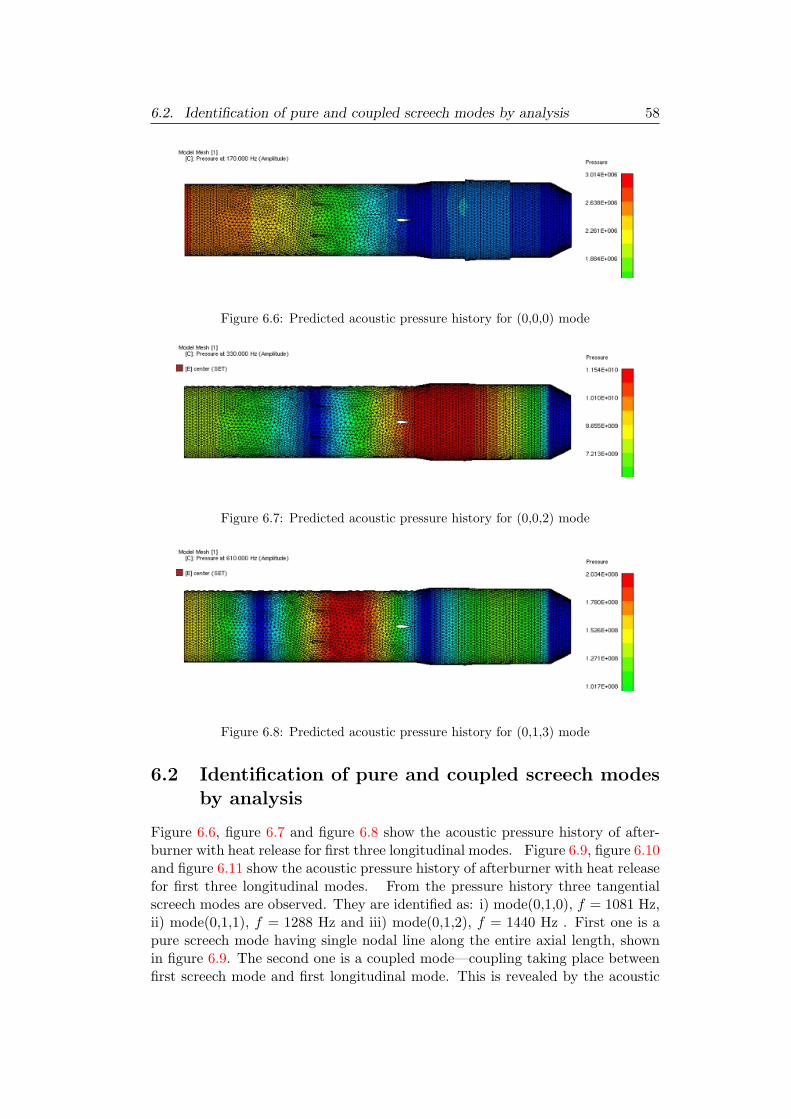
6.2. Identification of pure and coupled screech modes by analysis 58
Figure 6.6: Predicted acoustic pressure history for (0,0,0) mode
Figure 6.7: Predicted acoustic pressure history for (0,0,2) mode
Figure 6.8: Predicted acoustic pressure history for (0,1,3) mode
6.2 Identification of pure and coupled screech modesby analysis
Figure 6.6, figure 6.7 and figure 6.8 show the acoustic pressure history of after-burner with heat release for first three longitudinal modes. Figure 6.9, figure 6.10and figure 6.11 show the acoustic pressure history of afterburner with heat releasefor first three longitudinal modes. From the pressure history three tangentialscreech modes are observed. They are identified as: i) mode(0,1,0), f = 1081 Hz,ii) mode(0,1,1), f = 1288 Hz and iii) mode(0,1,2), f = 1440 Hz . First one is apure screech mode having single nodal line along the entire axial length, shownin figure 6.9. The second one is a coupled mode—coupling taking place betweenfirst screech mode and first longitudinal mode. This is revealed by the acoustic
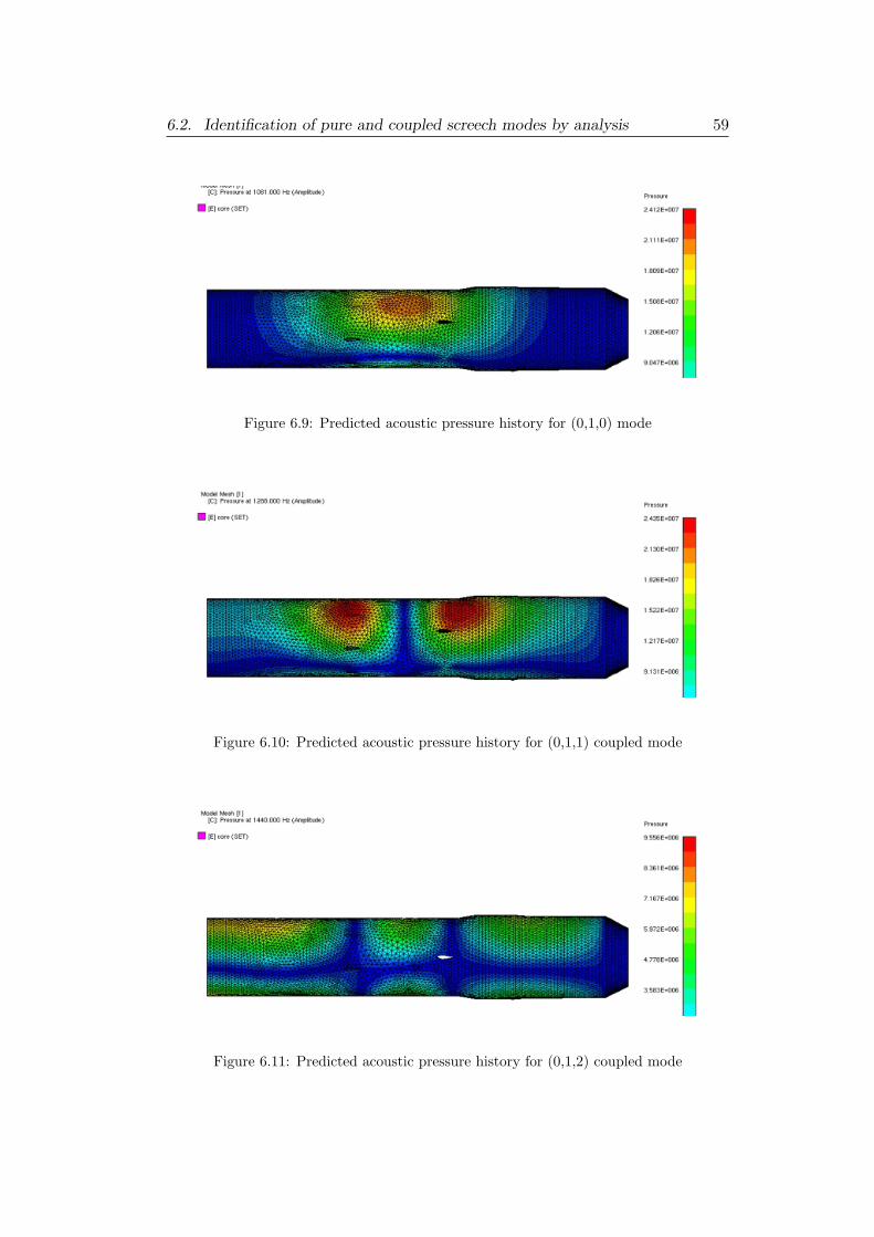
6.2. Identification of pure and coupled screech modes by analysis 59
Figure 6.9: Predicted acoustic pressure history for (0,1,0) mode
Figure 6.10: Predicted acoustic pressure history for (0,1,1) coupled mode
Figure 6.11: Predicted acoustic pressure history for (0,1,2) coupled mode
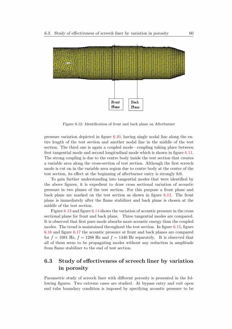
6.3. Study of effectiveness of screech liner by variation in porosity 60
Figure 6.12: Identification of front and back plane on Afterburner
pressure variation depicted in figure 6.10, having single nodal line along the en-tire length of the test section and another nodal line in the middle of the testsection. The third one is again a coupled mode—coupling taking place betweenfirst tangential mode and second longitudinal mode which is shown in figure 6.11.The strong coupling is due to the centre body inside the test section that createsa variable area along the cross-section of test section. Although the first screechmode is cut on in the variable area region due to centre body at the centre of thetest section, its effect at the beginning of afterburner entry is strongly felt.
To gain further understanding into tangential modes that were identified bythe above figures, it is expedient to draw cross sectional variation of acousticpressure in two planes of the test section. For this purpose a front plane andback plane are marked on the test section as shown in figure 6.12. The frontplane is immediately after the flame stabilizer and back plane is chosen at themiddle of the test section.
Figure 6.13 and figure 6.14 shows the variation of acoustic pressure in the crosssectional plane for front and back plane. Three tangential modes are compared.It is observed that first pure mode absorbs more acoustic energy than the coupledmodes. The trend is maintained throughout the test section. In figure 6.15, figure6.16 and figure 6.17 the acoustic pressure at front and back planes are comparedfor f = 1081 Hz, f = 1288 Hz and f = 1440 Hz separately. It is observed thatall of them seem to be propagating modes without any reduction in amplitudefrom flame stabilizer to the end of test section.
6.3 Study of effectiveness of screech liner by variationin porosity
Parametric study of screech liner with different porosity is presented in the fol-lowing figures. Two extreme cases are studied. At bypass entry and exit openend tube boundary condition is imposed by specifying acoustic pressure to be
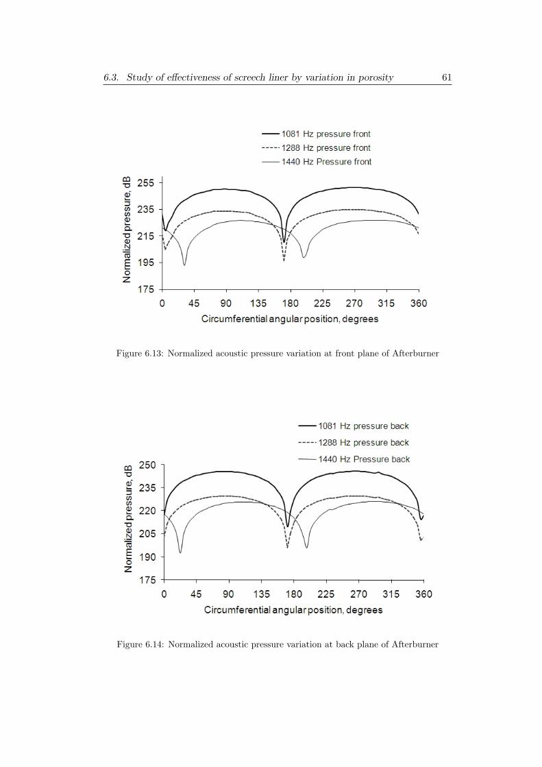
6.3. Study of effectiveness of screech liner by variation in porosity 61
Figure 6.13: Normalized acoustic pressure variation at front plane of Afterburner
Figure 6.14: Normalized acoustic pressure variation at back plane of Afterburner
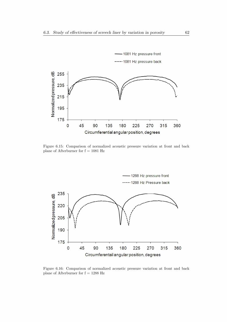
6.3. Study of effectiveness of screech liner by variation in porosity 62
Figure 6.15: Comparison of normalized acoustic pressure variation at front and backplane of Afterburner for f = 1081 Hz
Figure 6.16: Comparison of normalized acoustic pressure variation at front and backplane of Afterburner for f = 1288 Hz
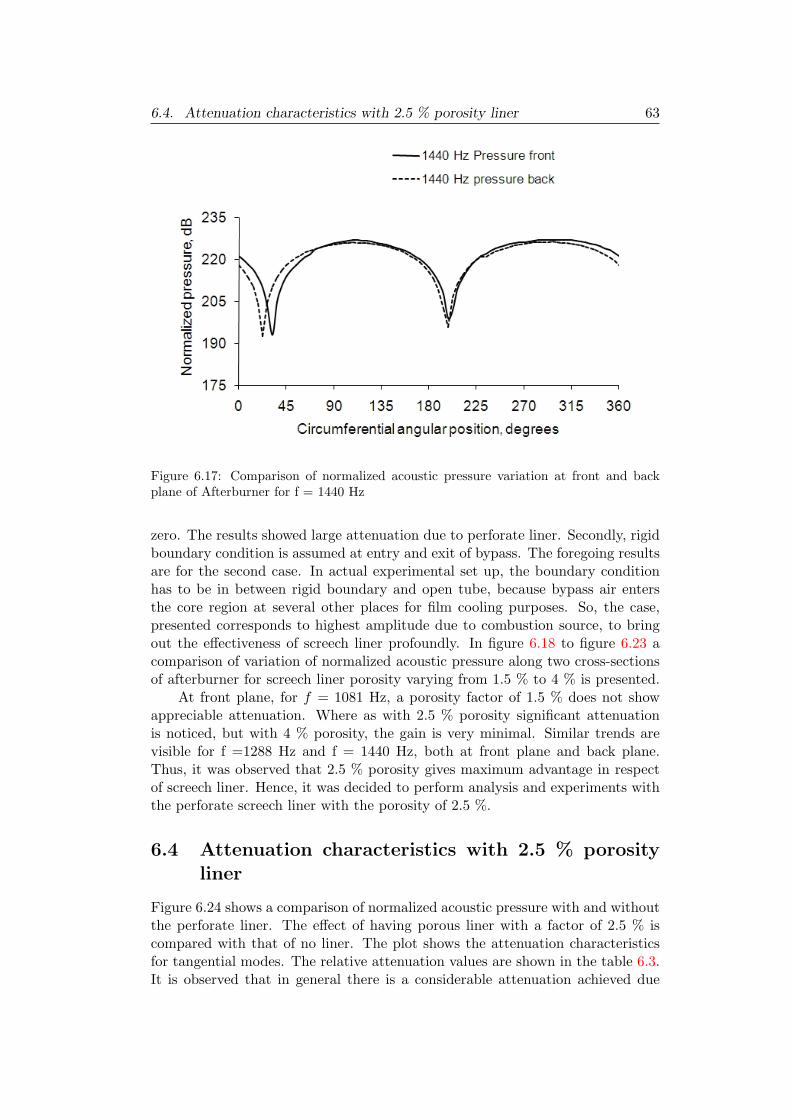
6.4. Attenuation characteristics with 2.5 % porosity liner 63
Figure 6.17: Comparison of normalized acoustic pressure variation at front and backplane of Afterburner for f = 1440 Hz
zero. The results showed large attenuation due to perforate liner. Secondly, rigidboundary condition is assumed at entry and exit of bypass. The foregoing resultsare for the second case. In actual experimental set up, the boundary conditionhas to be in between rigid boundary and open tube, because bypass air entersthe core region at several other places for film cooling purposes. So, the case,presented corresponds to highest amplitude due to combustion source, to bringout the effectiveness of screech liner profoundly. In figure 6.18 to figure 6.23 acomparison of variation of normalized acoustic pressure along two cross-sectionsof afterburner for screech liner porosity varying from 1.5 % to 4 % is presented.
At front plane, for f = 1081 Hz, a porosity factor of 1.5 % does not showappreciable attenuation. Where as with 2.5 % porosity significant attenuationis noticed, but with 4 % porosity, the gain is very minimal. Similar trends arevisible for f =1288 Hz and f = 1440 Hz, both at front plane and back plane.Thus, it was observed that 2.5 % porosity gives maximum advantage in respectof screech liner. Hence, it was decided to perform analysis and experiments withthe perforate screech liner with the porosity of 2.5 %.
6.4 Attenuation characteristics with 2.5 % porosityliner
Figure 6.24 shows a comparison of normalized acoustic pressure with and withoutthe perforate liner. The effect of having porous liner with a factor of 2.5 % iscompared with that of no liner. The plot shows the attenuation characteristicsfor tangential modes. The relative attenuation values are shown in the table 6.3.It is observed that in general there is a considerable attenuation achieved due
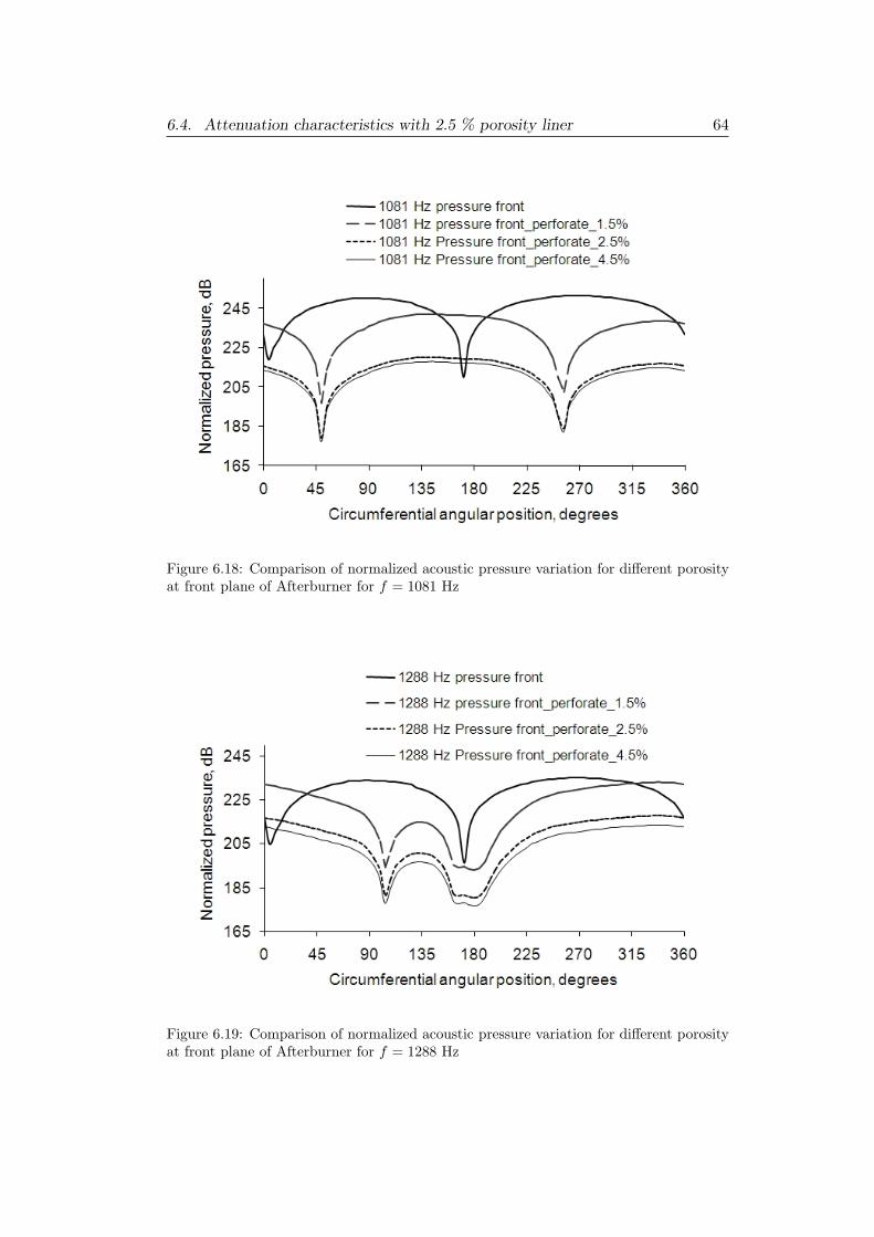
6.4. Attenuation characteristics with 2.5 % porosity liner 64
Figure 6.18: Comparison of normalized acoustic pressure variation for different porosityat front plane of Afterburner for f = 1081 Hz
Figure 6.19: Comparison of normalized acoustic pressure variation for different porosityat front plane of Afterburner for f = 1288 Hz
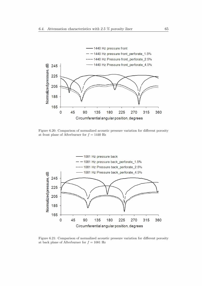
6.4. Attenuation characteristics with 2.5 % porosity liner 65
Figure 6.20: Comparison of normalized acoustic pressure variation for different porosityat front plane of Afterburner for f = 1440 Hz
Figure 6.21: Comparison of normalized acoustic pressure variation for different porosityat back plane of Afterburner for f = 1081 Hz
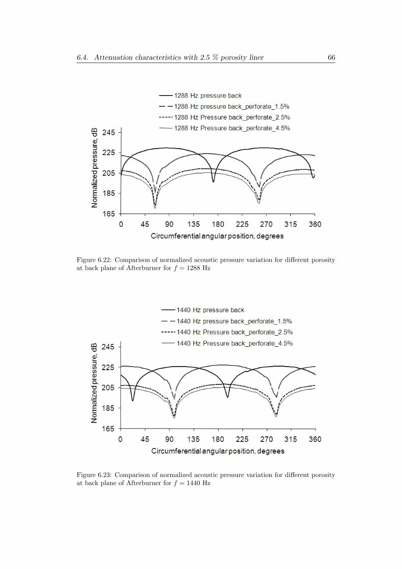
6.4. Attenuation characteristics with 2.5 % porosity liner 66
Figure 6.22: Comparison of normalized acoustic pressure variation for different porosityat back plane of Afterburner for f = 1288 Hz
Figure 6.23: Comparison of normalized acoustic pressure variation for different porosityat back plane of Afterburner for f = 1440 Hz
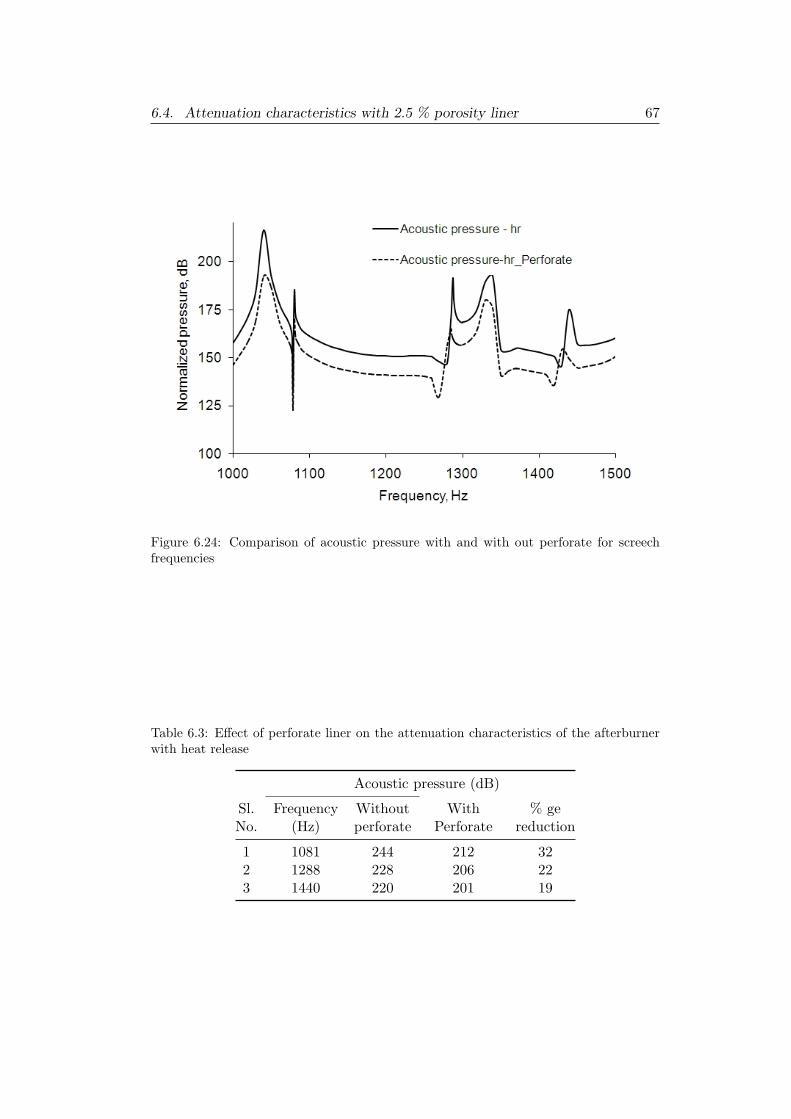
6.4. Attenuation characteristics with 2.5 % porosity liner 67
Figure 6.24: Comparison of acoustic pressure with and with out perforate for screechfrequencies
Table 6.3: Effect of perforate liner on the attenuation characteristics of the afterburnerwith heat release
Acoustic pressure (dB)
Sl. Frequency Without With % geNo. (Hz) perforate Perforate reduction
1 1081 244 212 322 1288 228 206 223 1440 220 201 19
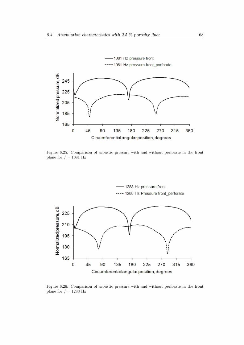
6.4. Attenuation characteristics with 2.5 % porosity liner 68
Figure 6.25: Comparison of acoustic pressure with and without perforate in the frontplane for f = 1081 Hz
Figure 6.26: Comparison of acoustic pressure with and without perforate in the frontplane for f = 1288 Hz
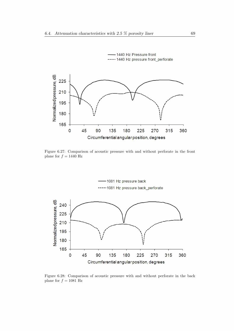
6.4. Attenuation characteristics with 2.5 % porosity liner 69
Figure 6.27: Comparison of acoustic pressure with and without perforate in the frontplane for f = 1440 Hz
Figure 6.28: Comparison of acoustic pressure with and without perforate in the backplane for f = 1081 Hz
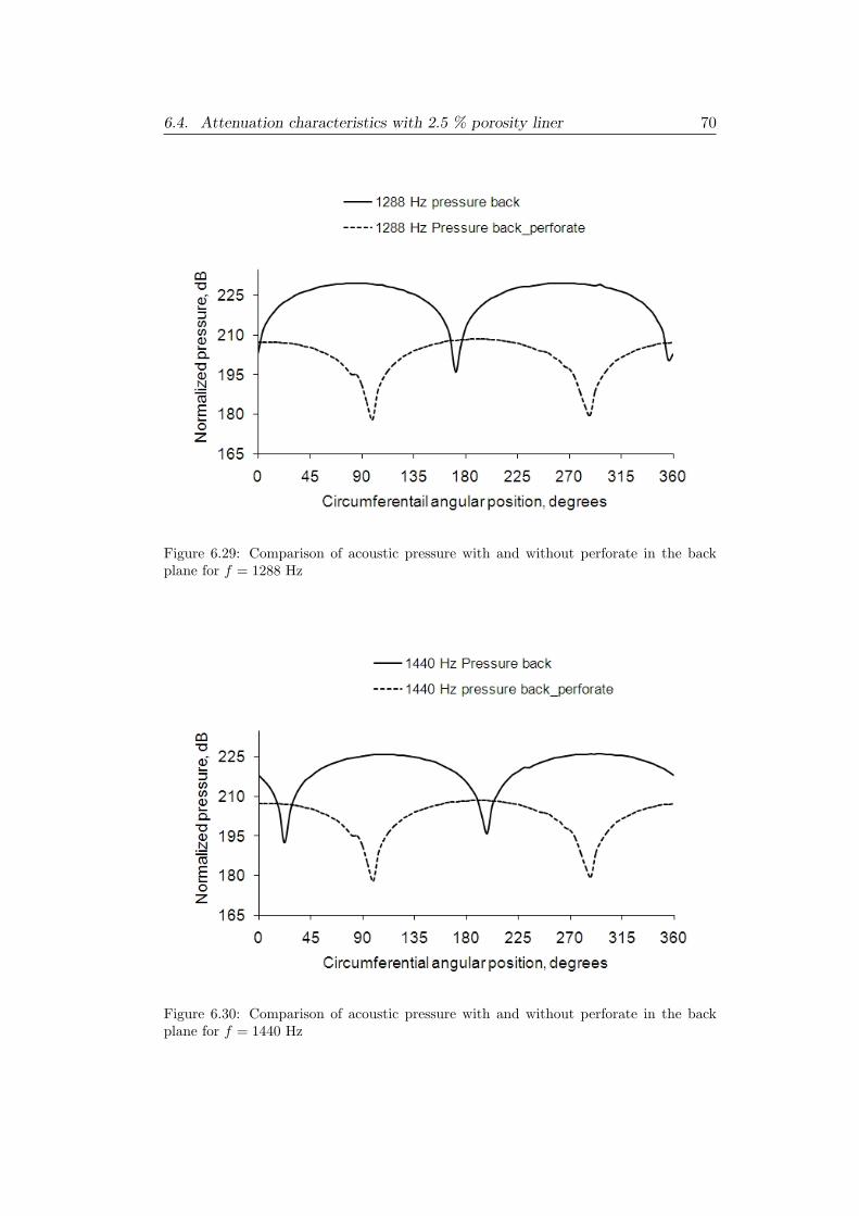
6.4. Attenuation characteristics with 2.5 % porosity liner 70
Figure 6.29: Comparison of acoustic pressure with and without perforate in the backplane for f = 1288 Hz
Figure 6.30: Comparison of acoustic pressure with and without perforate in the backplane for f = 1440 Hz
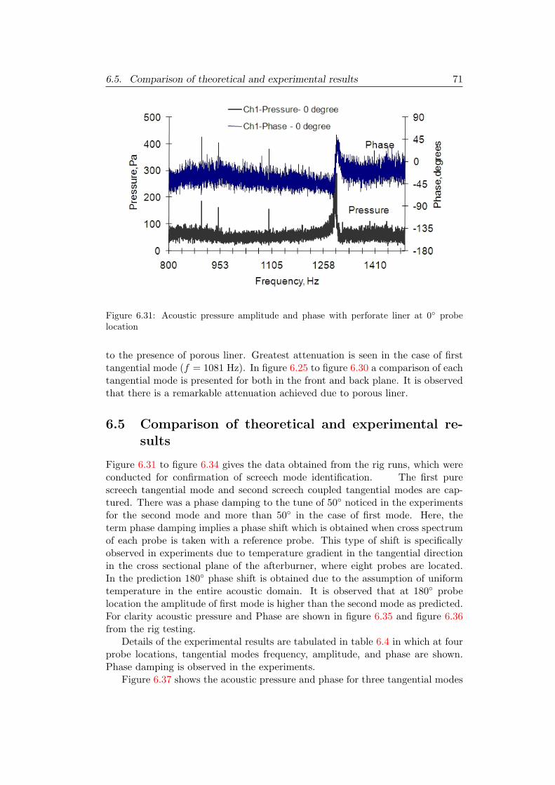
6.5. Comparison of theoretical and experimental results 71
Figure 6.31: Acoustic pressure amplitude and phase with perforate liner at 0 probelocation
to the presence of porous liner. Greatest attenuation is seen in the case of firsttangential mode (f = 1081 Hz). In figure 6.25 to figure 6.30 a comparison of eachtangential mode is presented for both in the front and back plane. It is observedthat there is a remarkable attenuation achieved due to porous liner.
6.5 Comparison of theoretical and experimental re-sults
Figure 6.31 to figure 6.34 gives the data obtained from the rig runs, which wereconducted for confirmation of screech mode identification. The first purescreech tangential mode and second screech coupled tangential modes are cap-tured. There was a phase damping to the tune of 50 noticed in the experimentsfor the second mode and more than 50 in the case of first mode. Here, theterm phase damping implies a phase shift which is obtained when cross spectrumof each probe is taken with a reference probe. This type of shift is specificallyobserved in experiments due to temperature gradient in the tangential directionin the cross sectional plane of the afterburner, where eight probes are located.In the prediction 180 phase shift is obtained due to the assumption of uniformtemperature in the entire acoustic domain. It is observed that at 180 probelocation the amplitude of first mode is higher than the second mode as predicted.For clarity acoustic pressure and Phase are shown in figure 6.35 and figure 6.36from the rig testing.
Details of the experimental results are tabulated in table 6.4 in which at fourprobe locations, tangential modes frequency, amplitude, and phase are shown.Phase damping is observed in the experiments.
Figure 6.37 shows the acoustic pressure and phase for three tangential modes
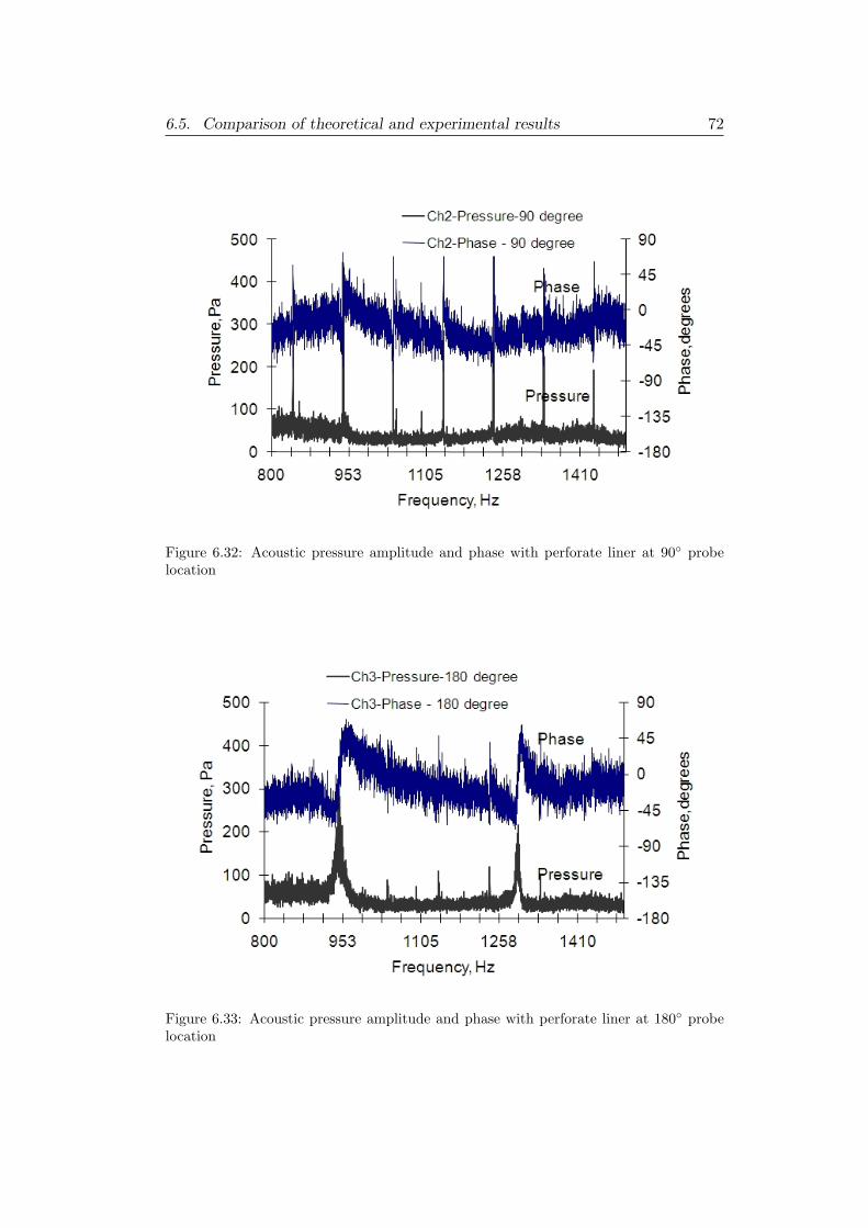
6.5. Comparison of theoretical and experimental results 72
Figure 6.32: Acoustic pressure amplitude and phase with perforate liner at 90 probelocation
Figure 6.33: Acoustic pressure amplitude and phase with perforate liner at 180 probelocation
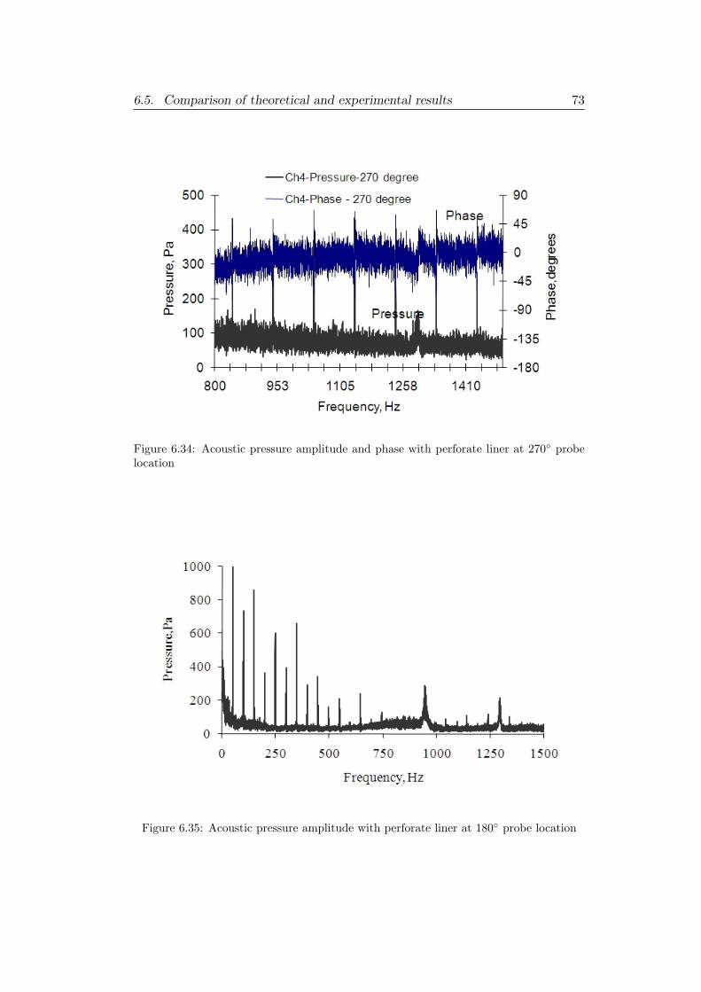
6.5. Comparison of theoretical and experimental results 73
Figure 6.34: Acoustic pressure amplitude and phase with perforate liner at 270 probelocation
Figure 6.35: Acoustic pressure amplitude with perforate liner at 180 probe location
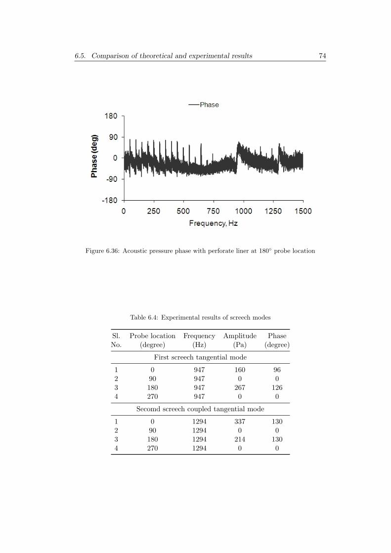
6.5. Comparison of theoretical and experimental results 74
Figure 6.36: Acoustic pressure phase with perforate liner at 180 probe location
Table 6.4: Experimental results of screech modes
Sl. Probe location Frequency Amplitude PhaseNo. (degree) (Hz) (Pa) (degree)
First screech tangential mode
1 0 947 160 962 90 947 0 03 180 947 267 1264 270 947 0 0
Secomd screech coupled tangential mode
1 0 1294 337 1302 90 1294 0 03 180 1294 214 1304 270 1294 0 0
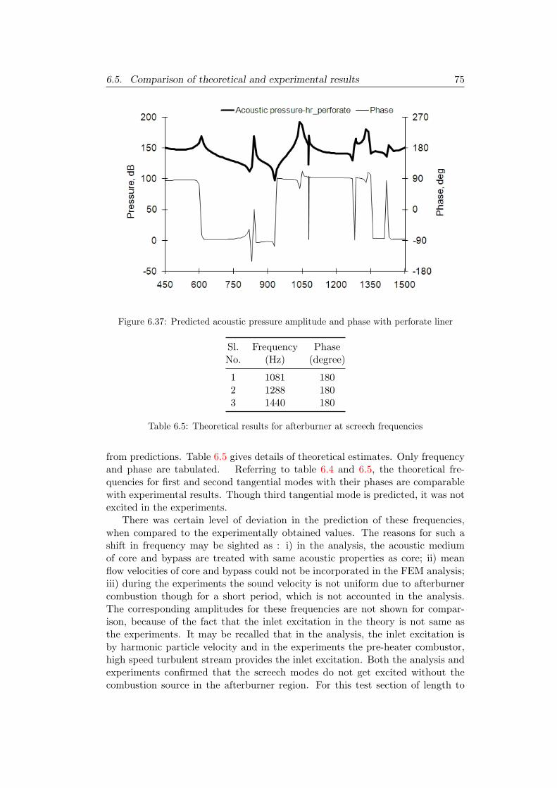
6.5. Comparison of theoretical and experimental results 75
Figure 6.37: Predicted acoustic pressure amplitude and phase with perforate liner
Sl. Frequency PhaseNo. (Hz) (degree)
1 1081 1802 1288 1803 1440 180
Table 6.5: Theoretical results for afterburner at screech frequencies
from predictions. Table 6.5 gives details of theoretical estimates. Only frequencyand phase are tabulated. Referring to table 6.4 and 6.5, the theoretical fre-quencies for first and second tangential modes with their phases are comparablewith experimental results. Though third tangential mode is predicted, it was notexcited in the experiments.
There was certain level of deviation in the prediction of these frequencies,when compared to the experimentally obtained values. The reasons for such ashift in frequency may be sighted as : i) in the analysis, the acoustic mediumof core and bypass are treated with same acoustic properties as core; ii) meanflow velocities of core and bypass could not be incorporated in the FEM analysis;iii) during the experiments the sound velocity is not uniform due to afterburnercombustion though for a short period, which is not accounted in the analysis.The corresponding amplitudes for these frequencies are not shown for compar-ison, because of the fact that the inlet excitation in the theory is not same asthe experiments. It may be recalled that in the analysis, the inlet excitation isby harmonic particle velocity and in the experiments the pre-heater combustor,high speed turbulent stream provides the inlet excitation. Both the analysis andexperiments confirmed that the screech modes do not get excited without thecombustion source in the afterburner region. For this test section of length to

6.5. Comparison of theoretical and experimental results 76
diameter ratio of 5, no radial modes are encountered both in the analysis andexperiments in the frequency range of interest.
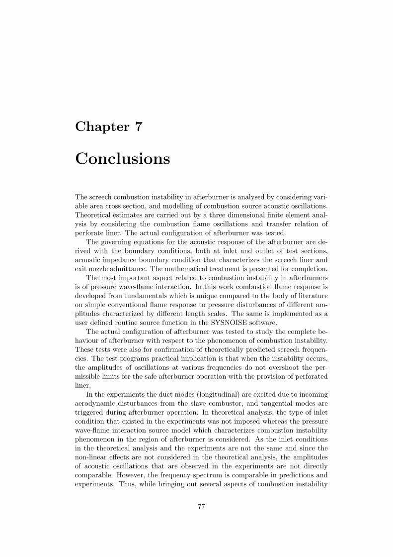
Chapter 7
Conclusions
The screech combustion instability in afterburner is analysed by considering vari-able area cross section, and modelling of combustion source acoustic oscillations.Theoretical estimates are carried out by a three dimensional finite element anal-ysis by considering the combustion flame oscillations and transfer relation ofperforate liner. The actual configuration of afterburner was tested.
The governing equations for the acoustic response of the afterburner are de-rived with the boundary conditions, both at inlet and outlet of test sections,acoustic impedance boundary condition that characterizes the screech liner andexit nozzle admittance. The mathematical treatment is presented for completion.
The most important aspect related to combustion instability in afterburnersis of pressure wave-flame interaction. In this work combustion flame response isdeveloped from fundamentals which is unique compared to the body of literatureon simple conventional flame response to pressure disturbances of different am-plitudes characterized by different length scales. The same is implemented as auser defined routine source function in the SYSNOISE software.
The actual configuration of afterburner was tested to study the complete be-haviour of afterburner with respect to the phenomenon of combustion instability.These tests were also for confirmation of theoretically predicted screech frequen-cies. The test programs practical implication is that when the instability occurs,the amplitudes of oscillations at various frequencies do not overshoot the per-missible limits for the safe afterburner operation with the provision of perforatedliner.
In the experiments the duct modes (longitudinal) are excited due to incomingaerodynamic disturbances from the slave combustor, and tangential modes aretriggered during afterburner operation. In theoretical analysis, the type of inletcondition that existed in the experiments was not imposed whereas the pressurewave-flame interaction source model which characterizes combustion instabilityphenomenon in the region of afterburner is considered. As the inlet conditionsin the theoretical analysis and the experiments are not the same and since thenon-linear effects are not considered in the theoretical analysis, the amplitudesof acoustic oscillations that are observed in the experiments are not directlycomparable. However, the frequency spectrum is comparable in predictions andexperiments. Thus, while bringing out several aspects of combustion instability
77
78
from experiments, the predicted modes (frequencies- longitudinal and tangential)are compared with experimental results, to validate theoretical development. Thefollowing conclusions are drawn:
1. Without the heat source only longitudinal acoustic modes are found to beexcited in the afterburner test section. With heat release, three additionaltangential modes are excited. Each mode is identified by the phase shift of180.
2. Since eight probes are provisioned in the circumferential cross section of af-terburner it was possible to identify the tangential modes by their respectivephase shift in the experiments.
3. From the pressure history three tangential screech modes are clearly iden-tified.
4. Two coupled tangential modes resulted due to variable area of the after-burner. It is observed that first pure mode absorbs more acoustic energythan the coupled modes. It is also observed that away from the flamestabilizer second coupled tangential mode shows reduction in amplitude.
5. Parametric study of screech liner porosity factor of 1.5 % has not shownappreciable attenuation. Where as with 2.5 % porosity significant attenu-ation is noticed, but with 4 % porosity, the gain is very minimal. Hence,the perforate screech liner with the porosity of 2.5 % is finalized. Greatestattenuation is seen in the case of first tangential mode.
6. From the rig runs, first pure screech tangential mode and second screechcoupled tangential modes are captured. There was a phase damping to thetune of 50 noticed in the experiments for the second mode and more than50 in the case of first mode. It is observed that at 180 probe location theamplitude of first mode is higher than the second mode as predicted.
7. The theoretical frequencies for first and second tangential modes with theirphases are comparable with experimental results. Though third tangentialmode is predicted, it was not excited in the experiments. There was certainlevel of deviation in the prediction of these frequencies, when compared tothe experimentally obtained values.
8. For this test section of length to diameter ratio of 5, no radial modes areencountered both in the analysis and experiments in the frequency rangeof interest.
9. The design inputs of screech liner are implemented in the actual engineafterburner. The tests of afterburner in the altitude standalone test facilityhave shown that the combustion instabilities amplitudes are with in thepermissible limits.
10. The exercise provides the expertise to analyse screech related problems dueto combustion source. When the experiments are quite difficult and costly
79
the analysis becomes the guideline for the confirmatory testing of afterburn-ers. It may be noted that triggering screech phenomenon itself is violentto the tune of 150 dB and data cannot be logged in for a longer duration,because when screech modes are cut-on, the amplitudes grow exponentiallyleading to structural failure. For this reason, theoretical estimates providea roadmap in the experiments to identify the screech modes quickly by on-line processing the data though for a short duration of the order 30 secondsor so.
In summary, an acoustic model has been developed for the afterburner com-bustor, taking into account the combustion response, the screech liner and thenozzle to study the acoustic instability of the afterburner. The flame responsemodel has been validated experimentally for longitudinal and tangential frequen-cies using a model test rig and the results have given sufficient confidence toapply the model for full scale afterburners as a predictive design tool. The ab-solute amplitudes cannot be predicted using the linear analysis presented here,which does not take into account the saturation effects. Further, the dampingeffects, such as droplet damping and viscous damping, are neglected in the anal-ysis. The future scope of work could be through CFD unsteady analysis whereeffect of many of these parameters could be evaluated and the magnitude effectscan also be predicted.
Appendix A
Nozzle Admittance
The theory of nozzle admittance was proposed by Crocco [68] in 1960 for rocketengines. This theory is adopted for the present work also. The analysis is repro-duced here for the sake of completeness.
A.1 Nozzle admittance for choked convergent nozzle
The behaviour of nozzle for non-isentropic, non-isothermal in the range of oscil-latory frequencies is given by using the continuity, momentum and energy equa-tions. Assuming the perturbations, p′, ρ′, and u′ to be small compared with theunperturbed quantities, the governing equations can be written in the followingform, retaining only the first order terms in the perturbations.
∂
∂t∗
(ρ′
ρ
)+ u
∂
∂z∗
(ρ′
ρ+u′
u
)= 0 (A.1)
∂
∂t∗
(u′
u
)+(ρ′
ρ+ 2
u′
u
)du
dz∗+ u
∂
∂z∗
(u′
u
)=p′
p
du
dz∗− p
ρu
∂
∂z∗
(p′
p
)(A.2)(
∂
∂t∗+ u
∂
∂z∗
)s′
cv=(∂
∂t∗+ u
∂
∂z∗
)(p′
p− γ ρ
′
ρ
)= 0 (A.3)
where z∗ is the distance along the nozzle and t∗ is the time. The energy equation iswritten expressing the constancy of entropy where s′ is the entropy perturbation,cv is the constant volume specific heat, and γ the adiabatic index.
In these equations u, du/dz∗ and p/ρu are known functions of z∗ determinedby the nozzle shape. Due to the linearity of the three equations above, theharmonic form of oscillatory time dependence is chosen and, using the complexrepresentation, the dependent variables are written as
p′/p = ϕ(z∗)ejωt∗; ρ′/ρ = σ(z∗)ejωt
∗; u′/u = ν(z∗)ejωt
∗(A.4)
where ω is the angular frequency of oscillation and ϕ, σ and ν are complexfunctions of z∗ alone. At the nozzle entrance, z∗ = z∗e , the three functions havecertain values ϕe, σe, νe. The boundary condition to be applied to the rest of theflow system as a result of the presence of nozzle is determined by the relationsbetween ϕe, σe, νe.
80
A.1. Nozzle admittance for choked convergent nozzle 81
Equation A.3 is integrated as
s′
cv=(p′
p− γ ρ
′
ρ
)= ψ
(t∗ −
∫ z∗
z∗e
dz∗
u
)(A.5)
where arbitrary function ψ being in general determined by the known time depen-dence of the entropy at z∗ = z∗e . For the exponential time dependence assumedin equations A.4
ϕ(z∗)− γσ(z∗) = ε exp
(−jω
∫ z∗
z∗e
dz∗
u
)(A.6)
where the constant ε represents the amplitude of the entropy oscillation dividedby cv. With the assumption A.4 and the relation A.5, equations A.1 and A.2 arereduced to the following system of ordinary differential equations in ν and σ.
udν
dz∗+ u
dσ
dz∗+ jωσ = 0 (A.7)
udν
dz∗+c∗2
u
dσ
dz∗+(
2du
dz+ jω
)ν − (γ − 1)
du
dz∗σ =
ε
(du
dz∗+ jω
c∗2
γu2
)exp
(−jω
∫ z∗
z∗e
dz∗
u
)(A.8)
An analytical solution is obtained by confining our domain to nozzle in which uincreases linearly with z∗ in the subsonic portion of the nozzle. Therefore,
du
dz∗=
u
z∗=c∗∗z∗∗
=c∗∗ − uelsub · L
(A.9)
in which c∗∗ represents the critical sound speed attained at the throat wherez∗ = z∗∗ , lsub = (z∗∗ − z∗e )/L represents the ratio of the length of the subsonicportion of the nozzle to the chamber length L. The subscript ∗ is used to denoteconditions at the nozzle throat.
Moreover a new independent variable is defined as
z = (z∗/z∗∗)2 = (u/c∗∗)
2 (A.10)
in terms of which
c∗2 = c∗∗2
12
(γ + 1)− 12
(γ − 1)z
(A.11)∫ z∗
z∗e
dz∗
u=
z∗∗2c∗∗
logz
ze(A.12)
where ze represents the assigned value of z at the nozzle entrance; and a reducedangular frequency is defined as
β =z∗∗ω
c∗∗=ωlsub · Lc∗∗ − ue
(A.13)
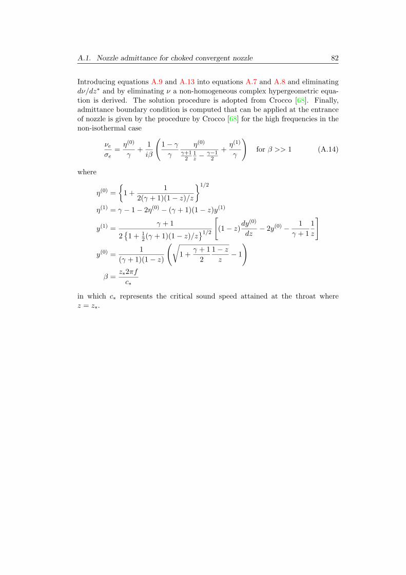
A.1. Nozzle admittance for choked convergent nozzle 82
Introducing equations A.9 and A.13 into equations A.7 and A.8 and eliminatingdν/dz∗ and by eliminating ν a non-homogeneous complex hypergeometric equa-tion is derived. The solution procedure is adopted from Crocco [68]. Finally,admittance boundary condition is computed that can be applied at the entranceof nozzle is given by the procedure by Crocco [68] for the high frequencies in thenon-isothermal case
νeσe
=η(0)
γ+
1iβ
(1− γγ
η(0)
γ+12
1z −
γ−12
+η(1)
γ
)for β >> 1 (A.14)
where
η(0) =
1 +1
2(γ + 1)(1− z)/z
1/2
η(1) = γ − 1− 2η(0) − (γ + 1)(1− z)y(1)
y(1) =γ + 1
2
1 + 12(γ + 1)(1− z)/z
1/2
[(1− z)dy
(0)
dz− 2y(0) − 1
γ + 11z
]
y(0) =1
(γ + 1)(1− z)
(√1 +
γ + 12
1− zz− 1
)
β =z∗2πfc∗
in which c∗ represents the critical sound speed attained at the throat wherez = z∗.
Bibliography
[1] J. L. Edwards. Reheat for gas turbines. Journal of the Royal AeronauticalSociety, 59(530):127–150, 1955.
[2] Anon. Summsummary of preliminary investigations into the characteris-tics of combustion screech in ducted flames. Technical Report NACA RME54B02, Lewis Laboratory, 1954.
[3] B. T. Lundin, D. S. Gabriel, and W. A. Fleming. Summary of NACA researchon afterburners. Technical Report RM E 55 L12, NACA, 1955.
[4] F. A. Williams. Combustion Theory. Combustion Science and EngineeringSeries. Persues Books, Cambridge, Massachusetts, 2 edition, 1985.
[5] T. J. Poinsot, A. C. Trouve, D. P. Veynate, S. M. Candel, and E. J. Esposito.Vortex driven acoustically coupled combustion instabilities. Journal of FluidMechanics, 177:265–292, 1987.
[6] K. Yu, A. Trouve, and J. Daily. Low-frequency pressure oscillation in amodel ramjet combustor. Journal of Fluid Mechanics, 232:47–72, 1991.
[7] C. J. Lawn, S. Evesque, and W. Polifke. A model for the thermoacousticresponse of a premixed swirl burner, Part I, Acoustic aspects. CombustionScience and Technology, 176:1331–1358, 2004.
[8] A. A. Putnam. Combustion-Driven Oscillations in industry. American ELSavier Publishers, New York, 1971.
[9] P. J. Longhorne. Reheat buzz: An acoustically coupled combustion instabil-ity, Part I, Experiment. Journal of Fluid Mechanics, 193:417–443, 1988.
[10] G. J. Bloxidge, A. P. Dowling, and P. J. Langhorne. Reheat buzz—an acous-tically coupled combustion instability, part II, Theory. Journal of FluidMechanics,, 193:445–473, 1988.
[11] A. P. Dowling. The calculation of thermoacoustic oscillations. Journal ofSound and Vibrations, 180:557–581, 1995.
[12] T. C. Lieuwen and J. H. Cho. Modeling the response of premixed flames dueto mixture ratio perturbations. Technical Report GT-2003-38089, ASMETurbo Expo, Atlanta, Georgia, USA, 2003.
83
Bibliography 84
[13] T. Sacarini and C. Freeman. The propagation of a fuel-air ratio disturbancein a simple premixer and its influence on pressure wave amplification. Tech-nical Report GT-2000-0106, ASME Turbo Expo, Munich, Germany, 2000.
[14] T. Sacarini, C. Freeman, and I. Day. Passive control of combustion instabilityin a low emission aeroderivative gas turbine. Technical Report GT-2004-53767, ASME Turbo Expo, Vienna, Austria, 2004.
[15] D.E. Rogers and F. E. Marble. A mechanism for high frequency oscillationsin ramjet combustors and afterburners. Jet propulsion, 1:456–462, 1956.
[16] F. E. C. Culick and K. Magiawalla. Excitation of acoustic modes in a cham-ber by vortex shedding. Journal of Sound and Vibrations, 64:455–457, 1979.
[17] K. Mateev and F. E. C. Culick. A model for combustion instability involvingvortex shedding. Combustion Science and Technology, 175:1059–1083, 2003.
[18] B. T. Chu. On the energy transfer to small disturbances in fluid flow. PartI. Acta Mechanica, 1:215–234, 1965.
[19] W. Polifke, C. O. Paschereit, and K. Dobbeling. Constructive and destructiveinterference of acoustic and entropy waves in premixed combustor with achoked exit. International Journal of Acoustics and Vibration, 6:135–146,2001.
[20] S. M. Candel and T. J. Poinsot. Interactions between and acoustics andcombustion. Proceedings of the Institute of Acoustics, pages 103–153, 1988.
[21] A. P. Dowling and G. J. Bloxidge. Reheat buzz—an acoustically drivencombustion instability. AIAA Paper, AIAA-84-2321, 1984.
[22] M. A. Macquisten and A. P. Dowling. Combustion oscillations in a twin-stream afterburner. Journal of Sound and Vibrations, 188:545–550, 1995.
[23] S. Sivasegaram, B. E. Thompson, and J. H. Whitelaw. Acoustic characteri-zation relevant to gas turbine augmenters. Journal of Propulsion, 5:109–115,1989.
[24] A. P Dowling. Vortices, sound and flames — a damaging combination. TheAeronautical Journal, pages 105–116, 2000.
[25] A. P. Dowling. A kinematic model of a ducted flame. Journal of FluidMechanics, 394:51–72, 1999.
[26] S. J. Brookes, R. S. Cant, and A. P. Dowling. Modeling combustion insta-bilities using computasional fluid dynamics. ASME 99-GT-112, 1999.
[27] Christopher A. Fannin. Linear Modeling and Analyis of ThermoacousticInstabilities in a Gas Turbine Combustor. PhD thesis, Virginia PolytechnicInstitute and State University, 2000.
Bibliography 85
[28] L. H. James Jr., W. W. Velie, and L. Bryant. Investigation of combustionscreech and a method of control. Technical Report RM E53L24b, NACA,1953.
[29] Z. M. Ibrahim, F. A. Williams, and S. G. Buckley. A review of previousstudies of oscillatory combustion in gas turbines. Technical Report UCSD-CER-05-04, University of California, San Diego, 2005.
[30] Jean-Pierre Hathout. Thermoacoustic instability. In A. F.Ghoniem, editor,Fundamentals and Modeling in Combustion, pages 1–10. MIT-2.280, 1999.
[31] Sebastien Ducruix, Thierry Schuller, and Daniel Durox. Combustion dynam-ics and instabilities: Elementary coupling and driving mechanisms. Journalof Propulsion and Power, 19:722–734, 2003.
[32] Jacob J. Keller. Thermoacoustic oscillations in combustion chambers of gasturbines. AIAA Journal, 33:2280–2287, 1995.
[33] Valter Bellucci, Bruno Schuermans, Dariusz Nowak, and Peter Flohr. Ther-moacoustic modeling of a gas turbine combustor equipped with acousticdampers. Transactions of ASME, 127:372–379, 2005.
[34] Ann P. Dowling and Simon R. Stow. Acoustic analyis of gas turbine com-bustors. Journal of Propulsion and Power, 19(5), 2003.
[35] G. Searby and D. Rochwerger. A parametric acoustic instability in premixedflames. Journal of Fluid Mechanics, 231:529–543, 1991.
[36] F. E. C. Culick. Short communication : A note on rayleigh’s criterion.Combustion Science and Technology, 56:159–166, 1987.
[37] J. G. Lee and D. A. Santavicca. Experimental diagnostics for the study ofcombustion instabilities in lean premixed combustors. Journal of Propulsionand Power, 19:735–749, 2003.
[38] T. Lieuwen. Modelling premixed combustion — acoustic wave interactions:a review. Journal of Propulsion and Power, 19(5):765–775, 2003.
[39] M. Fleifil, A. M. Annaswamy, Z. A. Ghoneim, and A. F. Ghoneim. Re-sponse of a laminar premixed flame to flow oscillations: A kinematic modeland thermoacoustic instability results. Combustion and Flame, 106:487–510,1996.
[40] J. F. Clarke. Finite amplitude waves in combustible gases. In J. D. Buckmas-ter, editor, Mathematics of Combustion, chapter 5, pages 183–245. SIAM,1985.
[41] A. C. McIntosh. Pressure disturbances of different length scales interactingwith conventional flames. Combustion Science and Technology, 75:287–309,1991.
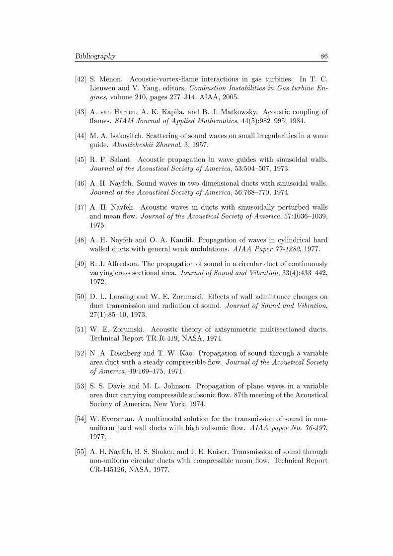
Bibliography 86
[42] S. Menon. Acoustic-vortex-flame interactions in gas turbines. In T. C.Lieuwen and V. Yang, editors, Combustion Instabilities in Gas turbine En-gines, volume 210, pages 277–314. AIAA, 2005.
[43] A. van Harten, A. K. Kapila, and B. J. Matkowsky. Acoustic coupling offlames. SIAM Journal of Applied Mathematics, 44(5):982–995, 1984.
[44] M. A. Isakovitch. Scattering of sound waves on small irregularities in a waveguide. Akusticheskii Zhurnal, 3, 1957.
[45] R. F. Salant. Acoustic propagation in wave guides with sinusoidal walls.Journal of the Acoustical Society of America, 53:504–507, 1973.
[46] A. H. Nayfeh. Sound waves in two-dimensional ducts with sinusoidal walls.Journal of the Acoustical Society of America, 56:768–770, 1974.
[47] A. H. Nayfeh. Acoustic waves in ducts with sinusoidally perturbed wallsand mean flow. Journal of the Acoustical Society of America, 57:1036–1039,1975.
[48] A. H. Nayfeh and O. A. Kandil. Propagation of waves in cylindrical hardwalled ducts with general weak undulations. AIAA Paper 77-1282, 1977.
[49] R. J. Alfredson. The propagation of sound in a circular duct of continuouslyvarying cross sectional area. Journal of Sound and Vibration, 33(4):433–442,1972.
[50] D. L. Lansing and W. E. Zorumski. Effects of wall admittance changes onduct transmission and radiation of sound. Journal of Sound and Vibration,27(1):85–10, 1973.
[51] W. E. Zorumski. Acoustic theory of axisymmetric multisectioned ducts.Technical Report TR R-419, NASA, 1974.
[52] N. A. Eisenberg and T. W. Kao. Propagation of sound through a variablearea duct with a steady compressible flow. Journal of the Acoustical Societyof America, 49:169–175, 1971.
[53] S. S. Davis and M. L. Johnson. Propagation of plane waves in a variablearea duct carrying compressible subsonic flow. 87th meeting of the AcousticalSociety of America, New York, 1974.
[54] W. Eversman. A multimodal solution for the transmission of sound in non-uniform hard wall ducts with high subsonic flow. AIAA paper No. 76-497,1977.
[55] A. H. Nayfeh, B. S. Shaker, and J. E. Kaiser. Transmission of sound throughnon-uniform circular ducts with compressible mean flow. Technical ReportCR-145126, NASA, 1977.
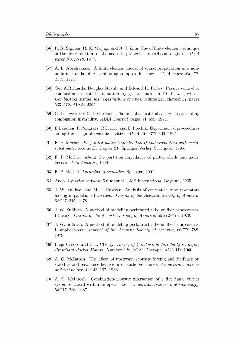
Bibliography 87
[56] R. K. Sigman, R. K. Majjigi, and B. J. Zinn. Use of finite element techniquein the determination of the acoustic properties of turbofan engines. AIAApaper No.77-18, 1977.
[57] A. L. Abrahamson. A finite element model of sound propagation in a non-uniform circular duct containing compressible flow. AIAA paper No. 77-1301, 1977.
[58] Geo A.Richards, Douglas Straub, and Edward H. Robey. Passive control ofcombustion instabilities in stationary gas turbines. In T.C.Liewen, editor,Combustion instabilites in gas turbine engines, volume 210, chapter 17, pages533–579. AIAA, 2005.
[59] G. D. Lewis and G. D Garrison. The role of acoustic absorbers in preventingcombustion instability. AIAA Journal, pages 71–699, 1971.
[60] E Laudien, R Pongratz, R Pierro, and D Prechik. Experimental proceeduresaiding the design of acoustic cavities. AIAA, 169:377–399, 1995.
[61] F. P. Mechel. Perforated plates (circular holes) and resonators with perfo-rated plate, volume II, chapter 21. Springer Verlag, Stuttgard, 1995.
[62] F. P. Mechel. About the partition impedance of plates, shells and mem-branes. Acta Acustica, 1999.
[63] F. P. Mechel. Formulas of acoustics. Springer, 2001.
[64] Anon. Sysnoise software 5.6 manual. LMS International Belgium, 2005.
[65] J. W. Sullivan and M. J. Crocker. Analysis of concentric tube resonatorshaving unpartitioned cavities. Journal of the Acoustic Society of America,64:207–215, 1978.
[66] J. W. Sullivan. A method of modeling perforated tube muffler components.I theory. Journal of the Acoustic Society of America, 66:772–778, 1979.
[67] J. W. Sullivan. A method of modeling perforated tube muffler components.II applications. Journal of the Acoustic Society of America, 66:779–788,1979.
[68] Luigi Crocco and S. I. Cheng. Theory of Combustion Instability in LiquidPropellant Rocket Motors. Number 8 in AGARDograph. AGARD, 1960.
[69] A. C. McIntosh. The effect of upstream acoustic forcing and feedback onstability and resonance behaviour of anchored flames. Combustion Scienceand technology, 49:143–167, 1986.
[70] A. C. McIntosh. Combustion-acoustic interaction of a flat flame burnersystem enclosed within an open tube. Combustion Science and technology,54:217–236, 1987.
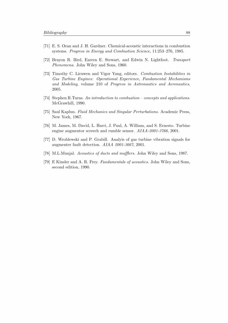
Bibliography 88
[71] E. S. Oran and J. H. Gardner. Chemical-acoustic interactions in combustionsystems. Progress in Energy and Combustion Science, 11:253–276, 1985.
[72] Brayon R. Bird, Earren E. Stewart, and Edwin N. Lightfoot. TransportPhenomena. John Wiley and Sons, 1960.
[73] Timothy C. Lieuwen and Vigor Yang, editors. Combustion Instabilities inGas Turbine Engines: Operational Experience, Fundamental Mechanismsand Modeling, volume 210 of Progress in Astronautics and Aeronautics,2005.
[74] Stephen R.Turns. An introduction to combustion – concepts and applications.McGrawhill, 1990.
[75] Saul Kaplun. Fluid Mechanics and Singular Perturbations. Academic Press,New York, 1967.
[76] M. James, M. David, L. Harri, J. Paul, A. William, and S. Ernesto. Turbineengine augmentor screech and rumble sensor. AIAA-2001-3766, 2001.
[77] D. Wroblewski and P. Grabill. Analyis of gas turbine vibration signals foraugmenter fault detection. AIAA 2001-3667, 2001.
[78] M.L.Munjal. Acoustics of ducts and mufflers. John Wiley and Sons, 1987.
[79] E Kinsler and A. R. Frey. Fundamentals of acoustics. John Wiley and Sons,second edition, 1990.