Embed Size (px)
Citation preview
Turbulent Premixed Combustion
Combustion Summer School
Prof. Dr.-Ing. Heinz Pitsch
2018
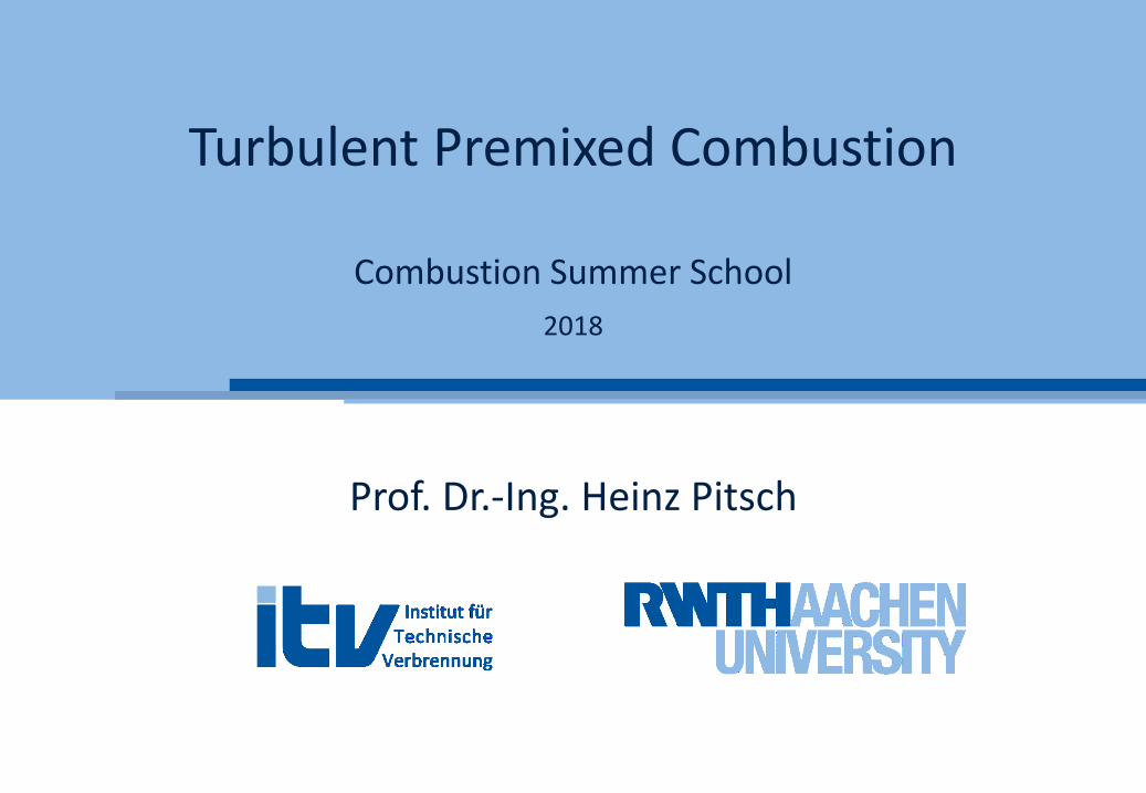
Example: LES of a stationary gas turbine
2
velocity field
flame
Course Overview
3
• Turbulence
• Turbulent Premixed Combustion
• Turbulent Non-Premixed
Combustion
• Turbulent Combustion Modeling
• Applications
• Scales of Turbulent Premixed
Combustion
• Regime-Diagram
• Turbulent Burning Velocity
Part II: Turbulent Combustion
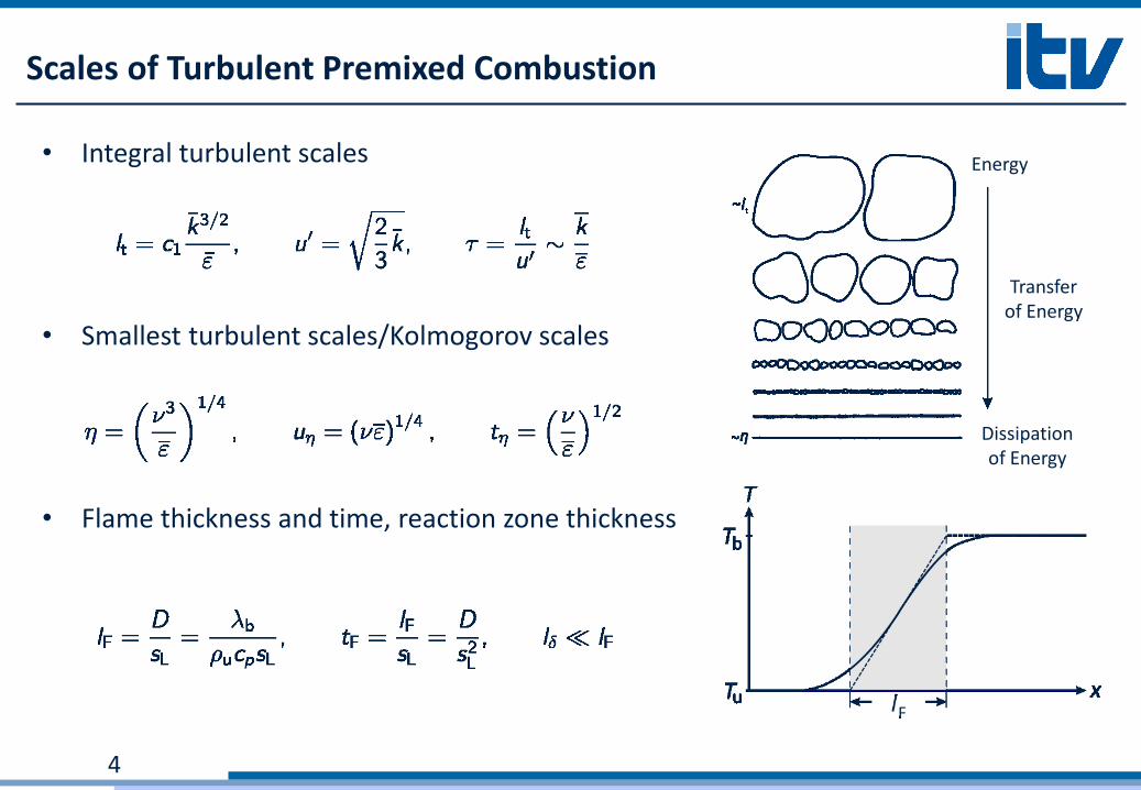
Scales of Turbulent Premixed Combustion
• Integral turbulent scales
• Smallest turbulent scales/Kolmogorov scales
• Flame thickness and time, reaction zone thickness
4
Energy
Transfer of Energy
Dissipation of Energy
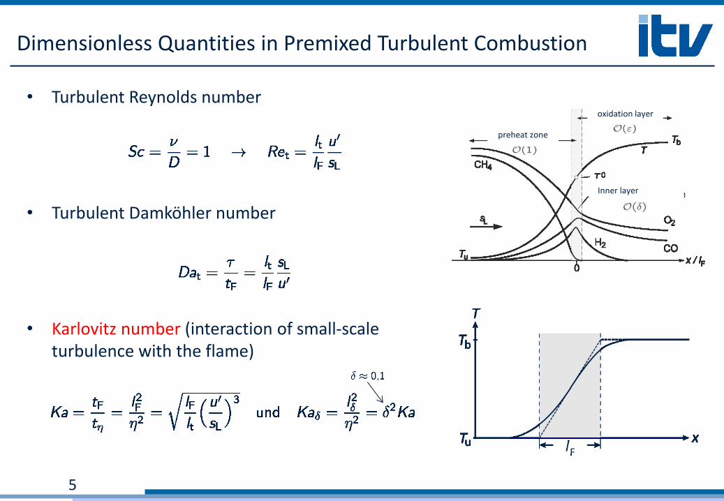
Dimensionless Quantities in Premixed Turbulent Combustion
• Turbulent Reynolds number
• Turbulent Damköhler number
• Karlovitz number (interaction of small-scale turbulence with the flame)
5
oxidation layer
preheat zone
Inner layer
Course Overview
6
• Turbulence
• Turbulent Premixed Combustion
• Turbulent Non-Premixed
Combustion
• Turbulent Combustion Modeling
• Applications
• Scales of Turbulent Premixed
Combustion
• Regime-Diagram
• Turbulent Burning Velocity
Part II: Turbulent Combustion
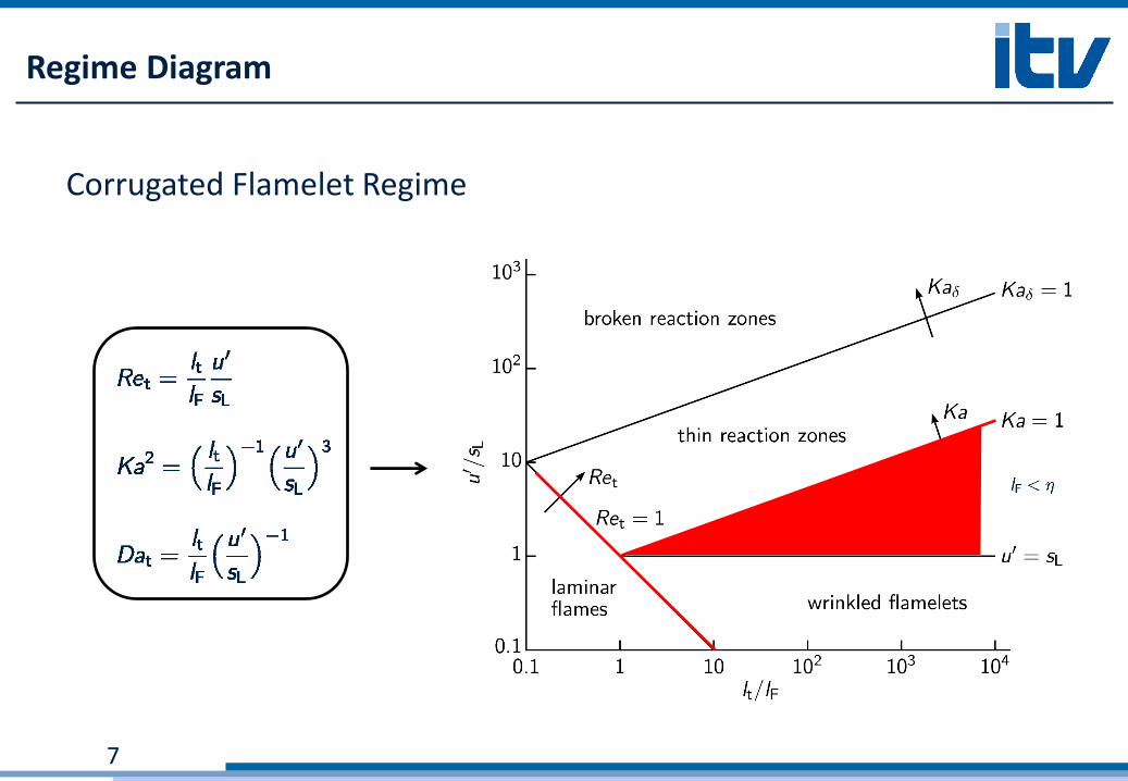
Regime Diagram
7
Corrugated Flamelet Regime
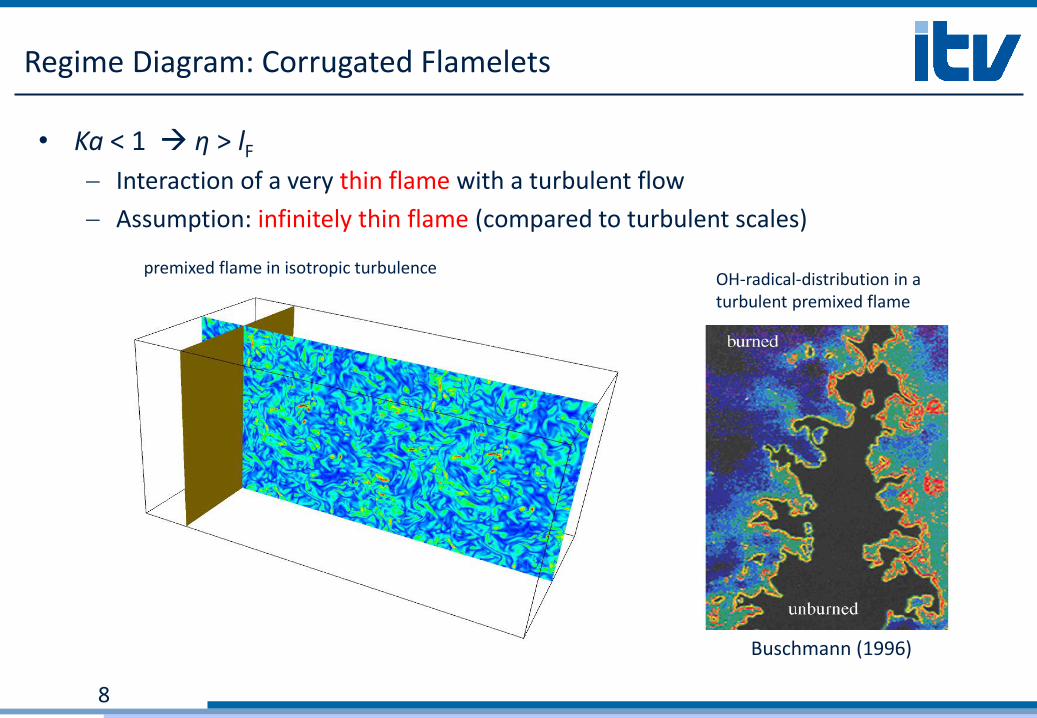
Regime Diagram: Corrugated Flamelets
• Ka < 1 η > lF
Interaction of a very thin flame with a turbulent flow
Assumption: infinitely thin flame (compared to turbulent scales)
8
Buschmann (1996)
OH-radical-distribution in a turbulent premixed flame
premixed flame in isotropic turbulence
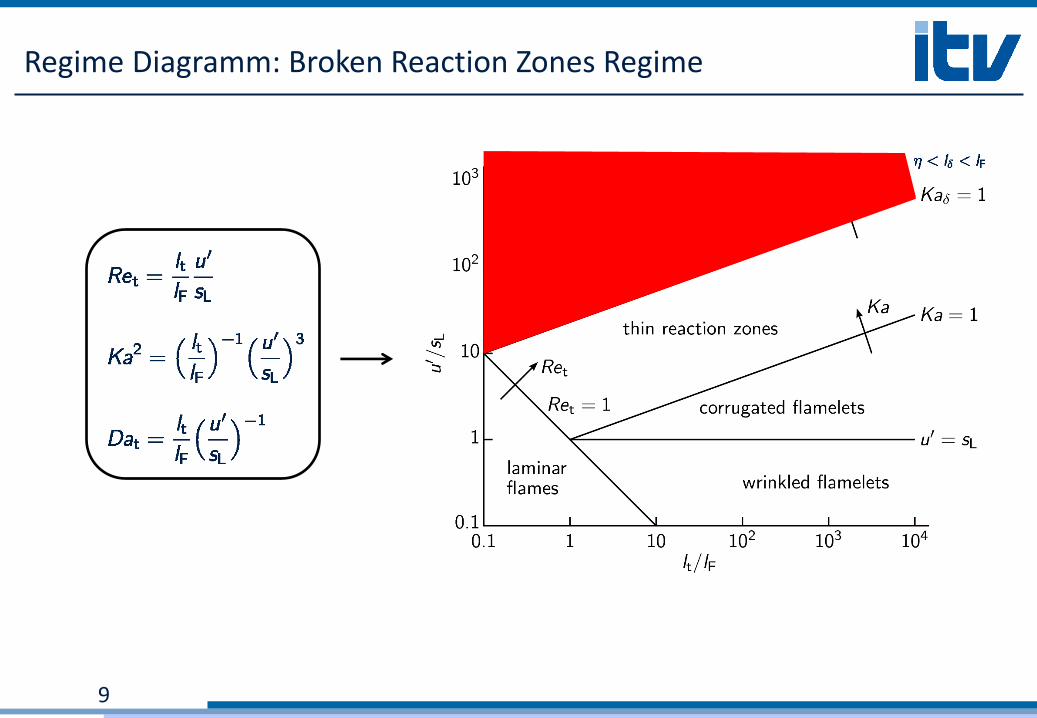
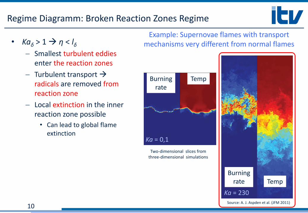
Regime Diagramm: Broken Reaction Zones Regime
9
Regime Diagramm: Broken Reaction Zones Regime
• Kaδ > 1 η < lδ
Smallest turbulent eddies enter the reaction zones
Turbulent transport radicals are removed from reaction zone
Local extinction in the inner reaction zone possible
• Can lead to global flame extinction
10
Two-dimensional slices from three-dimensional simulations
Ka = 0,1
Ka = 230
Source: A. J. Aspden et al. (JFM 2011)
Burning rate
Temp
Example: Supernovae flames with transport mechanisms very different from normal flames
Burning rate Temp
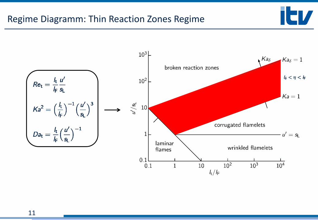
Regime Diagramm: Thin Reaction Zones Regime
11
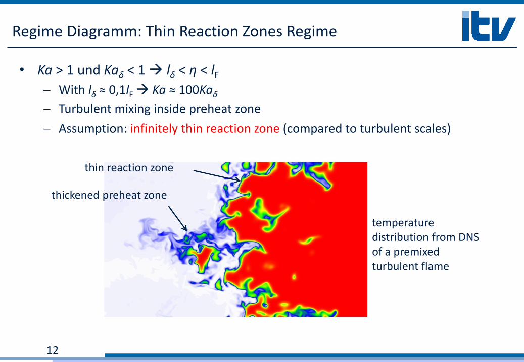
Regime Diagramm: Thin Reaction Zones Regime
12
thin reaction zone
thickened preheat zone
temperature distribution from DNS of a premixed turbulent flame
• Ka > 1 und Kaδ < 1 lδ < η < lF
With lδ ≈ 0,1lF Ka ≈ 100Kaδ
Turbulent mixing inside preheat zone
Assumption: infinitely thin reaction zone (compared to turbulent scales)
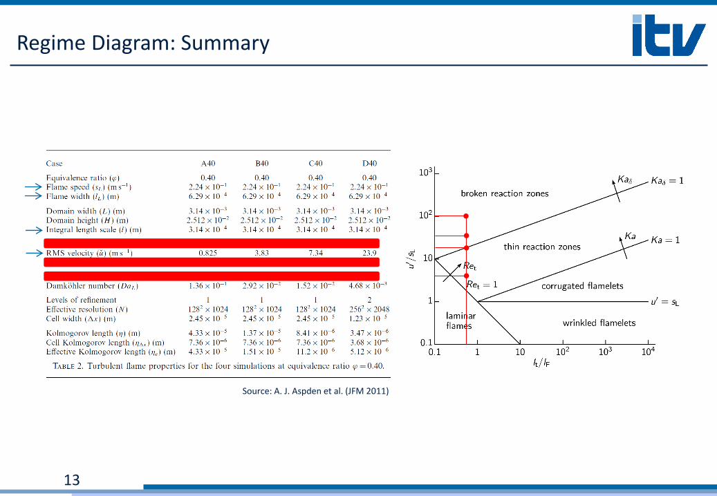
Regime Diagram: Summary
13
Source: A. J. Aspden et al. (JFM 2011)
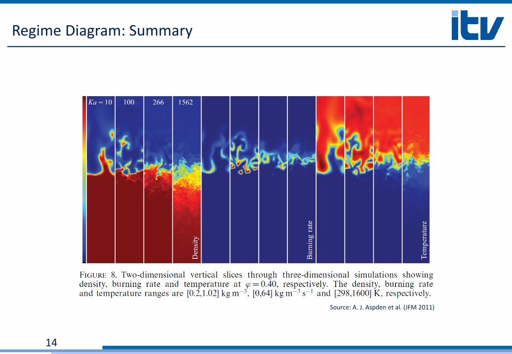
Regime Diagram: Summary
14
Source: A. J. Aspden et al. (JFM 2011)
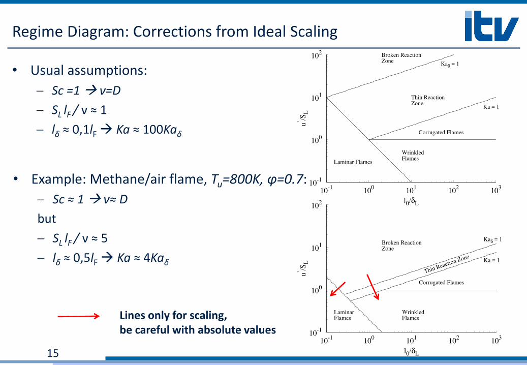
Regime Diagram: Corrections from Ideal Scaling
15
• Usual assumptions:
Sc =1 ν=D
SL lF / ν ≈ 1
lδ ≈ 0,1lF Ka ≈ 100Kaδ
• Example: Methane/air flame, Tu=800K, φ=0.7:
Sc ≈ 1 ν≈ D
but
SL lF / ν ≈ 5
lδ ≈ 0,5lF Ka ≈ 4Kaδ
Lines only for scaling, be careful with absolute values
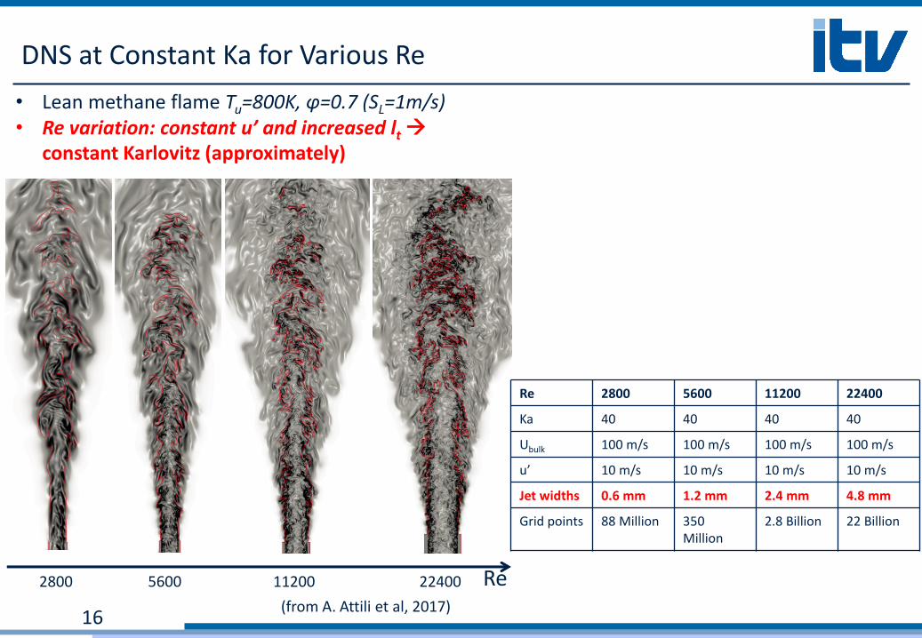
DNS at Constant Ka for Various Re
16 (from A. Attili et al, 2017)
• Lean methane flame Tu=800K, φ=0.7 (SL=1m/s) • Re variation: constant u’ and increased lt
constant Karlovitz (approximately)
Re 2800 11200 5600 22400
Re 2800 5600 11200 22400
Ka 40 40 40 40
Ubulk 100 m/s 100 m/s 100 m/s 100 m/s
u’ 10 m/s 10 m/s 10 m/s 10 m/s
Jet widths 0.6 mm 1.2 mm 2.4 mm 4.8 mm
Grid points 88 Million 350 Million
2.8 Billion 22 Billion
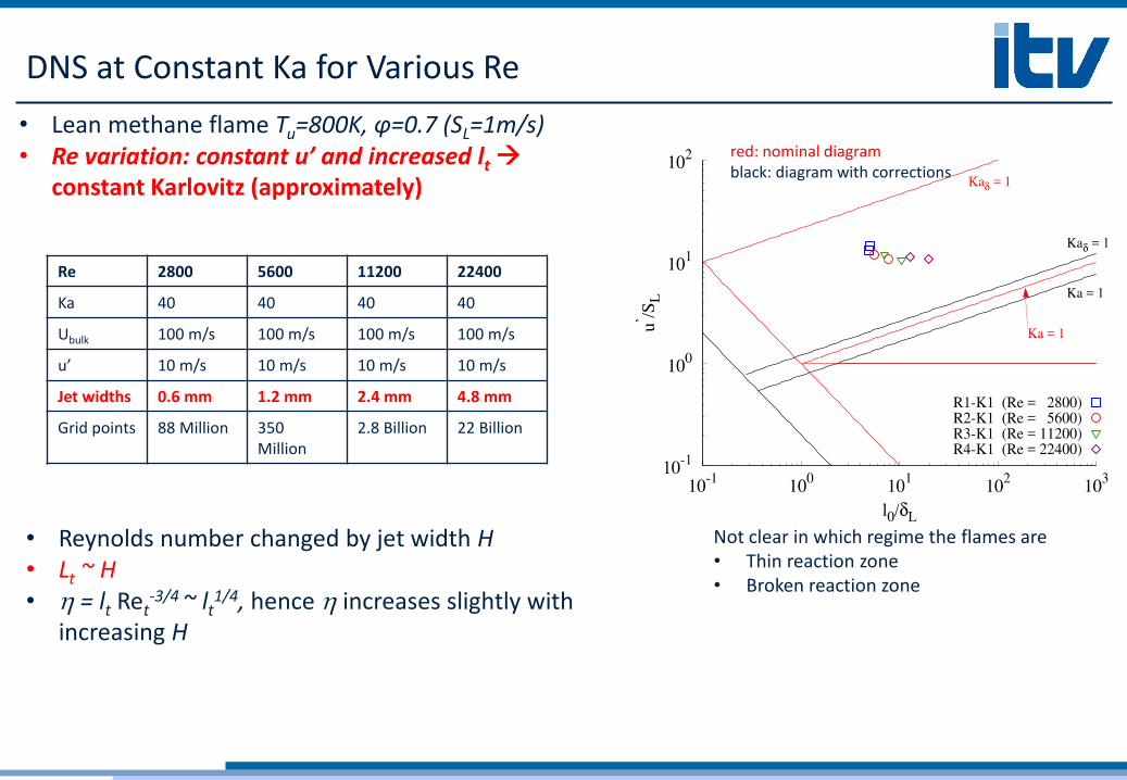
DNS at Constant Ka for Various Re
red: nominal diagram black: diagram with corrections
Re 2800 5600 11200 22400
Ka 40 40 40 40
Ubulk 100 m/s 100 m/s 100 m/s 100 m/s
u’ 10 m/s 10 m/s 10 m/s 10 m/s
Jet widths 0.6 mm 1.2 mm 2.4 mm 4.8 mm
Grid points 88 Million 350 Million
2.8 Billion 22 Billion
Not clear in which regime the flames are • Thin reaction zone • Broken reaction zone
• Lean methane flame Tu=800K, φ=0.7 (SL=1m/s) • Re variation: constant u’ and increased lt
constant Karlovitz (approximately)
• Reynolds number changed by jet width H • Lt ~ H • h = lt Ret
-3/4 ~ lt1/4, hence h increases slightly with
increasing H
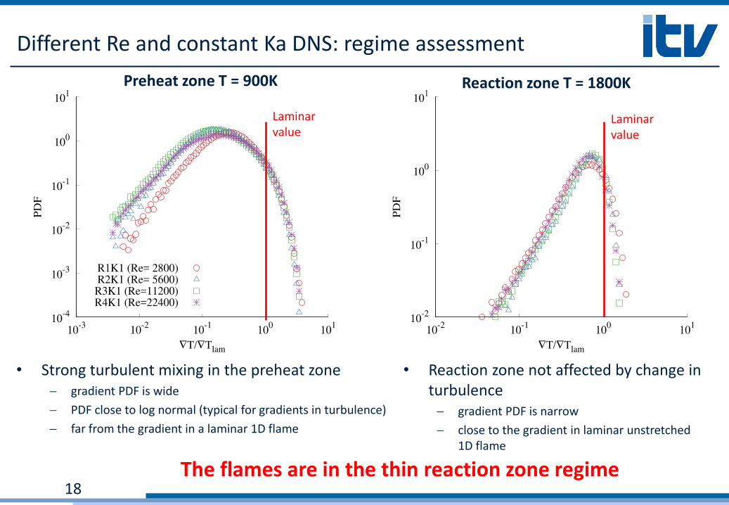
Different Re and constant Ka DNS: regime assessment
18
• Strong turbulent mixing in the preheat zone gradient PDF is wide
PDF close to log normal (typical for gradients in turbulence)
far from the gradient in a laminar 1D flame
Preheat zone T = 900K Reaction zone T = 1800K
Laminar value
Laminar value
• Reaction zone not affected by change in turbulence
gradient PDF is narrow
close to the gradient in laminar unstretched 1D flame
The flames are in the thin reaction zone regime
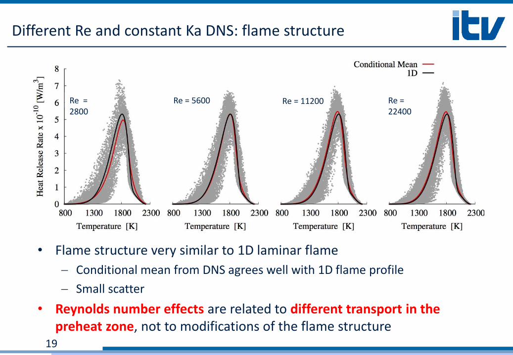
Different Re and constant Ka DNS: flame structure
19
Re = 2800
Re = 11200 Re = 5600 Re = 22400
• Flame structure very similar to 1D laminar flame
Conditional mean from DNS agrees well with 1D flame profile
Small scatter
• Reynolds number effects are related to different transport in the preheat zone, not to modifications of the flame structure

Course Overview
20
• Turbulence
• Turbulent Premixed Combustion
• Turbulent Non-Premixed
Combustion
• Turbulent Combustion Modeling
• Applications
• Scales of Turbulent Premixed
Combustion
• Regime-Diagram
• Turbulent Burning Velocity
Part II: Turbulent Combustion
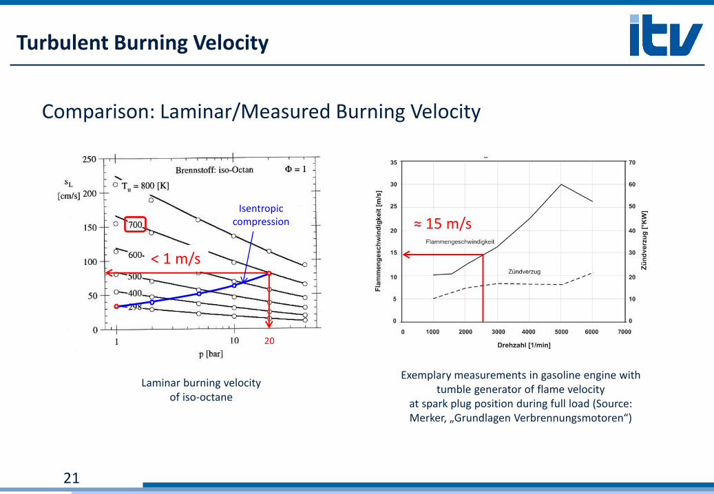
Turbulent Burning Velocity
21
Exemplary measurements in gasoline engine with tumble generator of flame velocity
at spark plug position during full load (Source: Merker, „Grundlagen Verbrennungsmotoren“)
Laminar burning velocity of iso-octane
≈ 15 m/s
< 1 m/s
20
Isentropic compression
Comparison: Laminar/Measured Burning Velocity
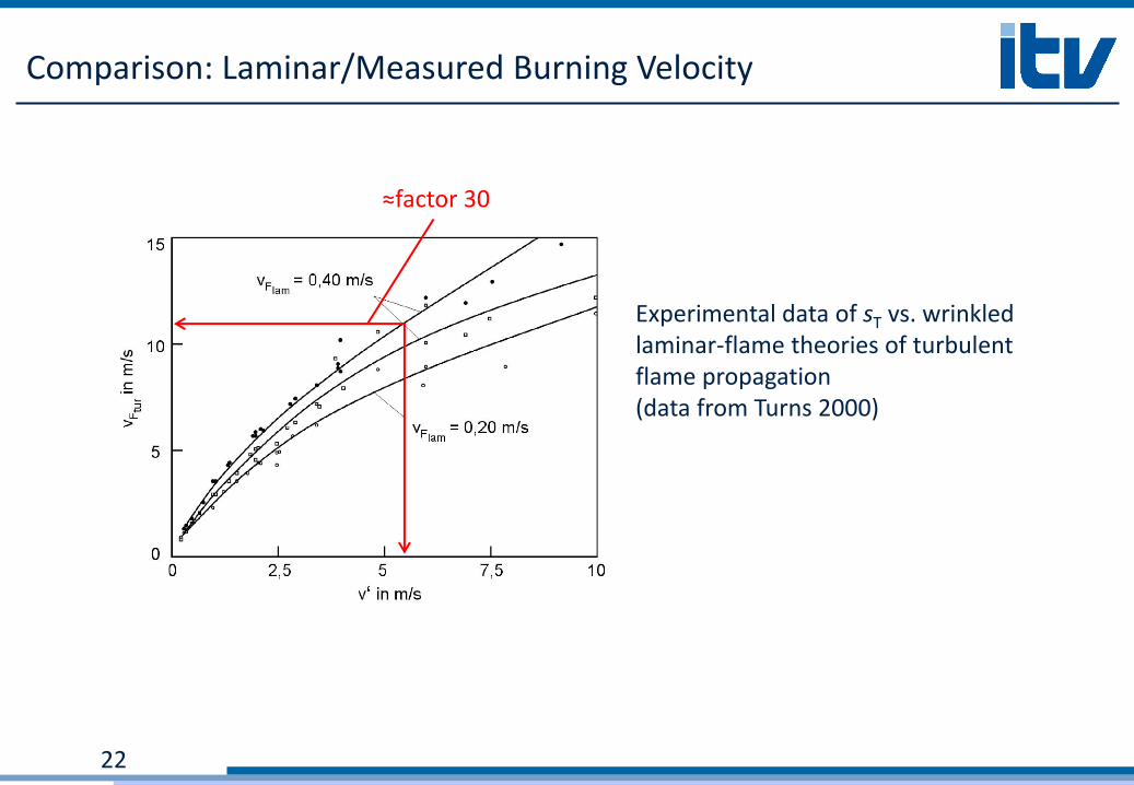
Comparison: Laminar/Measured Burning Velocity
22
Experimental data of sT vs. wrinkled laminar-flame theories of turbulent flame propagation (data from Turns 2000)
≈factor 30
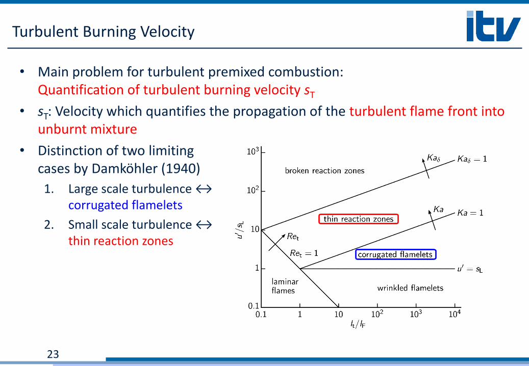
Turbulent Burning Velocity
• Main problem for turbulent premixed combustion: Quantification of turbulent burning velocity sT
• sT: Velocity which quantifies the propagation of the turbulent flame front into unburnt mixture
• Distinction of two limiting cases by Damköhler (1940)
1. Large scale turbulence ↔ corrugated flamelets
2. Small scale turbulence ↔ thin reaction zones
23
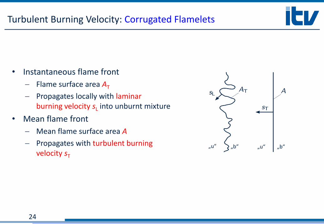
Turbulent Burning Velocity: Corrugated Flamelets
• Instantaneous flame front
Flame surface area AT
Propagates locally with laminar burning velocity sL into unburnt mixture
• Mean flame front
Mean flame surface area A
Propagates with turbulent burning velocity sT
24
„u“ „b“ „u“ „b“
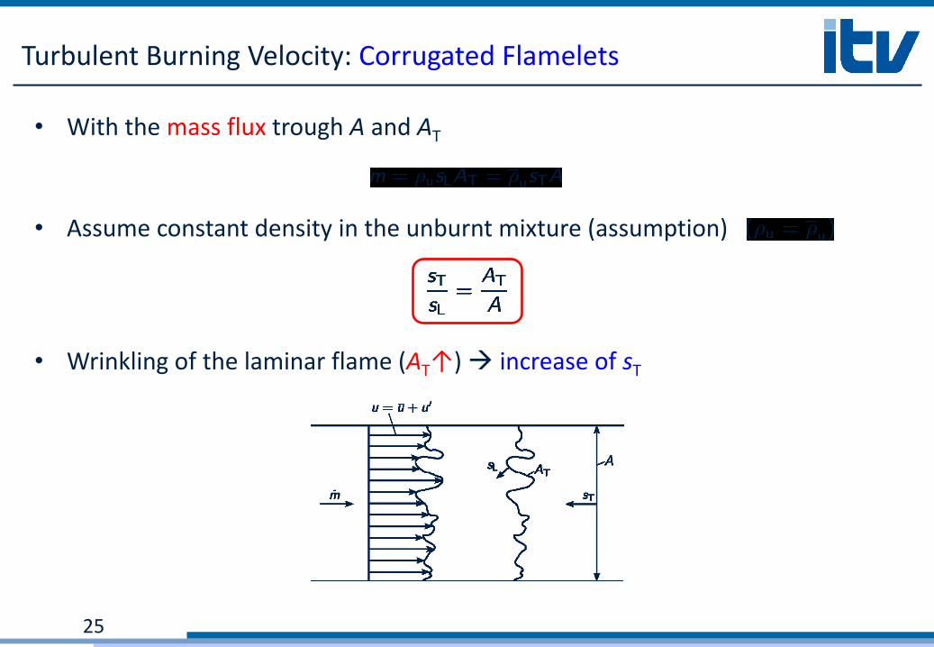
Turbulent Burning Velocity: Corrugated Flamelets
• With the mass flux trough A and AT
• Assume constant density in the unburnt mixture (assumption)
• Wrinkling of the laminar flame (AT↑) increase of sT
25
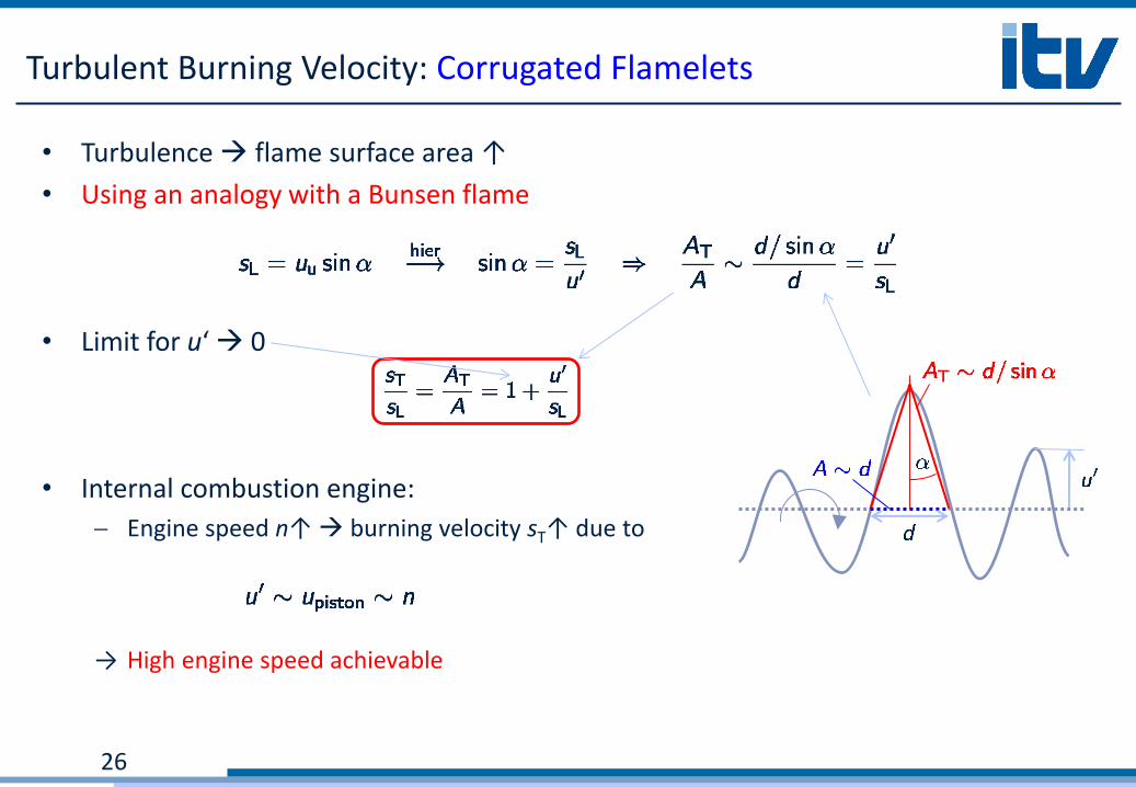
• Turbulence flame surface area ↑
• Using an analogy with a Bunsen flame
• Limit for u‘ 0
• Internal combustion engine:
Engine speed n↑ burning velocity sT↑ due to
→ High engine speed achievable
Turbulent Burning Velocity: Corrugated Flamelets
26
Turbulent Burning Velocity: large-scale turbulence
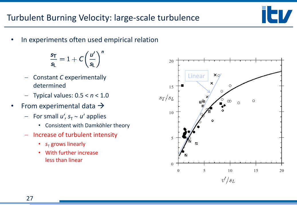
• In experiments often used empirical relation
Constant C experimentally determined
Typical values: 0.5 < n < 1.0
• From experimental data
For small u‘, sT ~ u‘ applies
• Consistent with Damköhler theory
Increase of turbulent intensity
• sT grows linearly
• With further increase less than linear
27
Linear
Turbulent Burning Velocity: Thin Reaction Zones
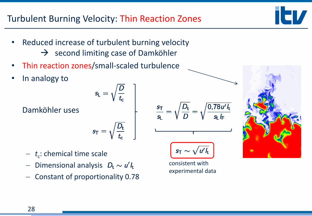
• Reduced increase of turbulent burning velocity second limiting case of Damköhler
• Thin reaction zones/small-scaled turbulence
• In analogy to Damköhler uses
tc: chemical time scale
Dimensional analysis
Constant of proportionality 0.78
28
consistent with experimental data
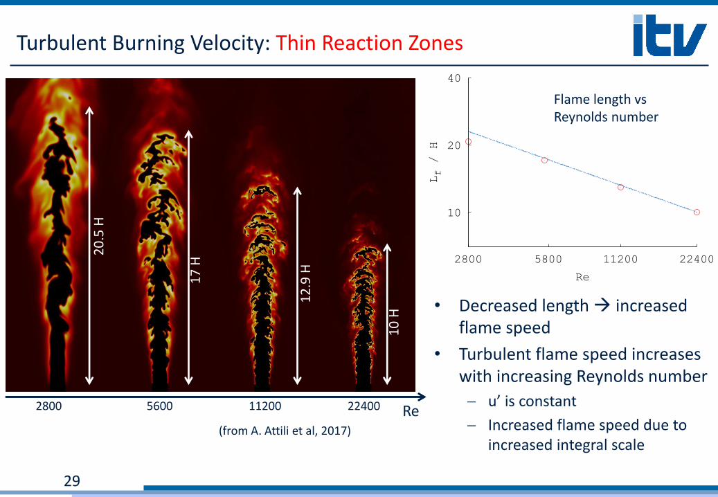
Turbulent Burning Velocity: Thin Reaction Zones
29
20
.5 H
10
H 1
2.9
H
17
H
Re 2800 11200 5600 22400
• Decreased length increased flame speed
• Turbulent flame speed increases with increasing Reynolds number
u’ is constant
Increased flame speed due to increased integral scale
(from A. Attili et al, 2017)
800
1000
1200
1400
1600
1800
2000
2200
0 1 2 3 4 5 6 7 8
T (K)
x (cm)
Re = 2800
Re = 5600
Re = 11200
Re = 22400
10
20
40
2800 5800 11200 22400
Lf / H
Re
Flame length vs Reynolds number
Turbulent Burning Velocity
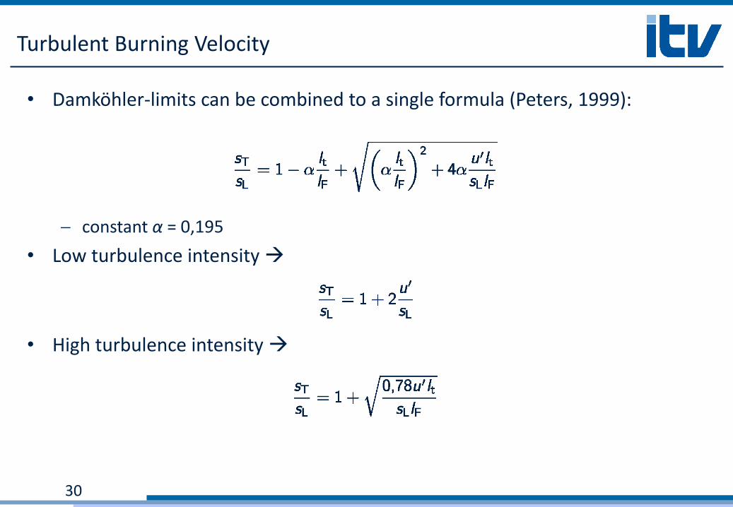
• Damköhler-limits can be combined to a single formula (Peters, 1999):
constant α = 0,195
• Low turbulence intensity
• High turbulence intensity
30
Turbulent Burning Velocity
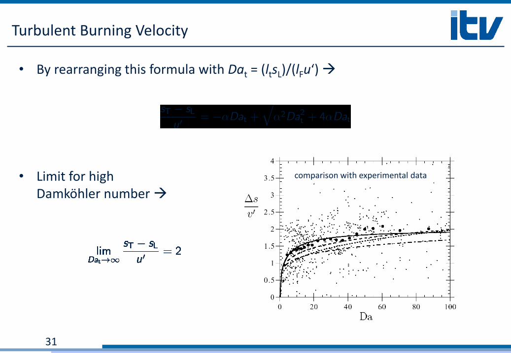
• By rearranging this formula with Dat = (ltsL)/(lFu‘)
• Limit for high Damköhler number
31
comparison with experimental data
Summary
32
• Turbulence
• Turbulent Premixed Combustion
• Turbulent Non-Premixed
Combustion
• Turbulent Combustion Modeling
• Applications
• Scales of Turbulent Premixed
Combustion
• Regime-Diagram
• Turbulent Burning Velocity
Part II: Turbulent Combustion