COMMENTARY NUMBER 508 Employment and Unemployment, … · Neither the Jobs Gain Nor the Unemployment-Rate Decline Was Meaningful February Unemployment: 7.7% (U.3), 14.3% (U.6), 23.0%

Copyright 2013 American Business Analytics & Research, LLC, www.shadowstats.com 1

COMMENTARY NUMBER 508 Employment and Unemployment, Money Supply, Consumer Credit

March 8, 2013

__________

Reflecting Ongoing, Seriously-Flawed Reporting, Neither the Jobs Gain Nor the Unemployment-Rate Decline Was Meaningful

February Unemployment: 7.7% (U.3), 14.3% (U.6), 23.0% (ShadowStats)

Consumer Credit Outstanding Remained Stagnant, Net of Federally-Held Student Loans

Slowing Growth in M3 Suggests Mounting Systemic Stress, As Monetary Base Continues to Soar

__________

PLEASE NOTE: The next regular Commentary is scheduled for Wednesday, March 13th, covering February retail sales, followed by a Commentary on Friday, March 15th, covering February industrial production, PPI, CPI and related inflation-adjusted series.

Detail on the January trade deficit, construction spending, household income and discussion on the relative investment performances of physical gold and stocks were published yesterday, March 7th, in an unscheduled Commentary No. 507.

Best wishes to all — John Williams

Shadow Government Statistics — Commentary No. 508, March 8, 2013


Opening Comments and Executive Summary. Following another round of seriously-flawed reporting out of the Bureau of Labor Statistics (BLS), the general outlook for U.S. economic conditions has not changed. As discussed in Special Commentary (No. 485), Hyperinflation 2012 and many weekly Commentaries, most of the available, better-quality economic reporting—both public and private—shows that the U.S. economic activity began to turn down in 2006 through 2007, plunged from late-2007 into mid-2009, and entered a period of protracted, low-level stagnation thereafter. The economy began turning down anew in second- or third-quarter 2012. There never was a recovery, and none is pending.

Given the official version of a December 2007-to-June 2009 recession; that was followed a by a recovery that topped pre-recession activity in fourth-quarter 2011; and that has seen ongoing growth ever since, the renewed downturn in the economy likely will be recognized (within the next 18 months or so) as being a second-dip in a double- or multiple-dip recession.

Beyond the happy labor data for February, the Open Comments and Executive Summary looks at February construction employment and January consumer credit outstanding. Consumer credit remained stagnant, net of the still-expanding level of student loans held by the federal government. In the Hyperinflation Watch section, slowing growth in February M3, a soaring monetary base and implications for mounting systemic stress are discussed.

February Employment and Unemployment. February’s headline labor numbers were positive, on the surface, but they were not meaningful, as increasingly has been the circumstance for some time.

Employment. On the jobs front, the issues involve upside biases built into the nonfarm payroll survey, as well as heavy distortions from highly-unstable monthly changes to the concurrent seasonal factor adjustments used in calculating the headline monthly change in payrolls. These problems are discussed extensively in Reporting Detail, in the Concurrent Seasonal Factor Distortions and Birth-Death/Bias Factor Adjustment sections.

The biases likely overstate monthly payroll change by at least 100,000 jobs per month. The concurrent seasonal factor distortions come from the BLS not publishing full revisions to the series each month, as the new adjusted numbers are calculated. As result, the just-published February jobs gain is not consistent or comparable with any reporting before December 2012. Given these circumstances, the margin of error in estimating month-to-month payroll change likely is much larger than the official 95% confidence interval of +/- 129,000. A more realistic number likely would encompass the headline 236,000 jobs gain reported for February.

Indeed February’s headline payroll employment gain was 236,000, versus a downwardly revised 119,000 monthly gain in January. Given the concerns mentioned above, neither the February nor January monthly gain likely was significant. Unaffected by the seasonal-adjustment games, however, not-seasonally-adjusted, year-to-year growth in payroll employment has been slowing. For February 2013, the year-to-year gain was 1.52%, versus a downwardly revised 1.52% in January and down from a revised 1.70% gain in December.

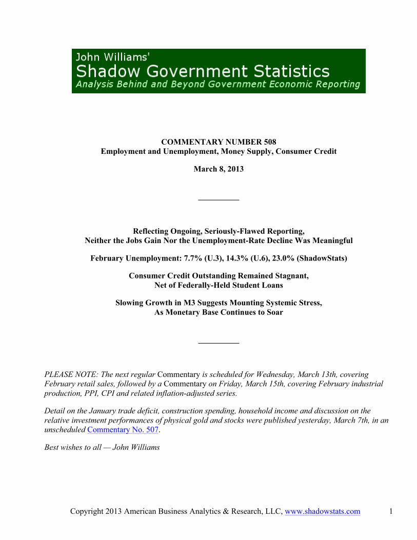
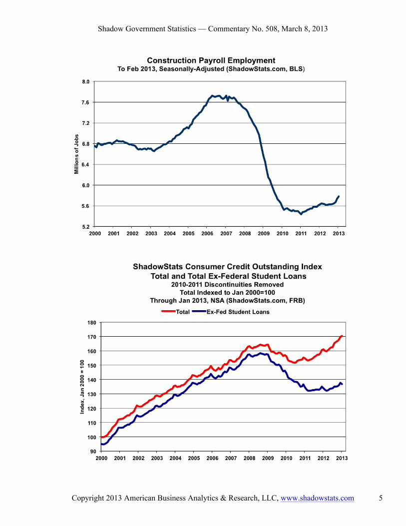
The first graph following is of seasonally-adjusted payroll levels since 2000. It shows current details of total nonfarm payroll employment levels, which still are well below the pre-2007 recession peak. The second graph is longer-term, showing historical detail back to 1940 and, in perspective, that payroll levels still are not that far ahead of the peak levels that preceded the 2001 recession.





Unemployment. On the unemployment front, the issues are definitional as well as tied to the unstable concurrent seasonal-factor adjustment process. The February headline U.3 unemployment rate came in at 7.74%, down by a statistically-insignificant 0.18% from the unrevised headline 7.92% rate in January. The headline data, however, measure only a subset of those who consider themselves to be unemployed, where an increasing portion of the labor force just cannot find a job.

The BLS’s broadest unemployment rate U.6 (including headline U.3 unemployment, short-term discouraged workers, and those working part-time because they cannot find a full-time job) eased to 14.3% in February, from 14.4% in January. Adding in long-term discouraged workers, the ShadowStats Alternate Unemployment measure held at its series-high of 23.0%, in February, for the third straight month.

A separate reporting problem here is that the month-to-month household survey data (unemployment-related) are not comparable. Concurrent seasonal adjustments are used to set the latest unemployment rate, for example, but that process also revises the prior and earlier months’ unemployment rates. The issue is that BLS does publish the revised data; it leaves the prior month’s reporting intact, and inconsistent with and not comparable to the latest data. Accordingly, month-to-month comparisons here simply are without meaning.

Both the definitional and concurrent-seasonal-adjustment issues for unemployment reporting are discussed more extensively in Reporting Detail, in the Household Survey Details section.

Other Reporting. Supplemental to the prior Commentary No. 507, construction employment has been updated through February, and consumer credit outstanding has been released for January 2013.

Construction Spending. Related to the discussion on construction spending in Commentary No. 507, today’s (March 8th) release of February 2013 payroll data by the BLS included February numbers for construction employment, as shown in the accompanying graph.

Seasonally-adjusted February construction jobs increased by 48,000 in the month to a total of 5.703 million. That followed a revised 25,000 (previously 30,000) gain estimated for January, but the estimated 38,000 monthly jobs gain in December versus November has no meaning. The November number is no longer consistent with December reporting, and month-to-month comparisons have no significance, given the BLS concurrent seasonal-factor adjustment and reporting policies discussed above and in Concurrent Seasonal Factors Distortions in the Reporting Detail section. Not-seasonally-adjusted numbers, however, are comparable on year-to-year basis, where year-to-year construction jobs growth in February picked up to 2.9%, from 2.0% in both January and December. To the extent these jobs gains are real, they likely have been tied to temporary boosts from broad weather conditions and from repair-and-replacement activity tied to damages from Hurricane Sandy.





Consumer Credit. The March 7th release by the Federal Reserve of January 2013 consumer credit outstanding confirmed the continuing and intensifying structural stresses on consumer liquidity. As shown in the preceding graph, the highly touted recent growth in total consumer credit outstanding—a factor viewed by some as a recovery in consumer liquidity and confidence—has been due solely to the extraordinary growth in federally-owned student loans, not in terms of bank lending that normally would help to stimulate retail sales and other consumption. Combined with a lack of real income growth, as discussed in Commentary No. 507, the lack of meaningful credit growth means that the consumer has no ability to support sustainable growth in personal consumption and housing, which account directly for 74% of the GDP, and which indirectly account for most of the remaining balance of broad economic activity.

The ShadowStats graph of Consumer Credit Outstanding was created by combining discontinuous series, published by the Federal Reserve, into a continuous index of activity, indexed to January 2000 = 100, as described in Commentary No. 501.

[More-complete details on the February labor data are found in the Reporting Detail section.]

HYPERINFLATION WATCH

February 2013 Broad Money Growth Slowed to 4.4%. Based on roughly three weeks of reported data, the preliminary estimate of year-to-year growth in the ShadowStats Ongoing-M3 Estimate for February 2013 is on track to hit 4.4%, down from a revised 4.6% (previously 4.5%) annual rate in January. The hard number will be published tomorrow (March 9th) in the Alternate Data tab at www.shadowstats.com.

Where annual growth had been on the upswing in recent months, the slowing growth in February likely is a sign of mounting systemic stress. As shown in the next section, the monetary base is soaring in response to Fed’s active and expanded QE3 but, as has been case for the current systemic-solvency crisis, the Fed’s actions have not flowed through to meaningful growth in the broad money supply. Bank lending remains troubled, and that is a signal of ongoing and, at this point, likely intensifying systemic stress.

Any prior-period revisions in the following numbers are due to Federal Reserve revisions to underlying data. The seasonally-adjusted, preliminary estimate of month-to-month change for the February 2013 money supply M3 is 0.1% contraction, versus a revised 0.6% (previously 0.5%) gain January. The estimated month-to-month M3 changes, however, remain less reliable than the estimates of annual growth.

For February 2013, early estimates of year-to-year and month-to-month changes follow for the narrower M1 and M2 measures (M2 includes M1, M3 includes M2). Full definitions are found in the Money Supply Special Report. M2 for February is estimated to show year-to-year growth of about 6.8%, down from an unrevised 7.5% in January, with month-to-month change estimated at roughly a 0.3% contraction, versus a revised monthly gain of 0.4% (previously 0.3%) in January. The early estimate of M1 for January is year-to-year growth of roughly 11.5%, down from a revised 11.8% (previously 11.6%) in January, with month-to-month February change a likely gain of 0.4%, versus a revised 0.8% (previously 0.7%) gain in January.





Monetary Base Keeps Expanding to Successive Record Levels. The monetary base, which is currency in circulation (part of M1 money supply) plus bank reserves (not part of the money supply) (see more-complete definition in the Money Supply Special Report), has continued to increase, fortnight after fortnight, to successive historic highs, in response to the Federal Reserve’s expanded QE3. The growing monetary base is shown in the preceding graphs, which are updated through March 6th.

Banks are parking their excess reserves with the Federal Reserve, not lending the available cash into the normal flow of commerce. When the Fed monetizes U.S. Treasury securities, as it has been doing, that usually adds directly to the broad money supply, and it contributes to selling pressure against the U.S. dollar. Faltering money supply growth in this circumstance, as discussed above, tends to indicate mounting systemic stress in the banking industry.

Hyperinflation Outlook: Summary. The next update of this section is planned along with the Commentary due for March 15th, which will cover February inflation and industrial production.

This summary is unchanged from Commentary No. 505, of February 22nd and is intended for new subscribers and for readers looking for a condensed version of the broad outlook or who otherwise are not familiar with the hyperinflation report or recent special commentaries, linked below. Those documents are suggested as background reading on the financial turmoil and currency upheaval facing the United States in the next year or two.

The November 27, 2012 Special Commentary (No. 485) updated Hyperinflation 2012 and the broad outlook for the economy and inflation, as well as for systemic stability and the U.S. dollar. These remain the two primary articles outlining current conditions and the background to the hyperinflation forecast. The basics have not changed here, other than events keep moving towards the circumstance of a domestic hyperinflation by the end of 2014. Nonetheless, a fully updated hyperinflation report is targeted for publication in the March to April time-frame.

The economic and systemic solvency crises of the last eight years continue. There never was an actual recovery following the economic downturn that began in 2006 and collapsed into 2008 and 2009. What followed was a protracted period of business stagnation that began to turn down anew in second- and third-quarter 2012. The official recovery seen in GDP has been a statistical illusion generated by the use of understated inflation in calculating key economic series. Nonetheless, the renewed downturn likely will gain recognition as the second-dip in a double- or multiple-dip recession.

What continues to unfold in the systemic and economic crises is just an ongoing part of the 2008 panic and near-collapse of the system at the time. All the extraordinary actions and interventions bought a little time, but they did not resolve the various crises. That the crises continue can be seen in deteriorating economic activity and in the panicked actions by the Federal Reserve, where it proactively is monetizing U.S. Treasury debt at a pace suggestive of a Treasury that is unable to borrow otherwise. As discussed in the Opening Comments section [of Commentary No. 505], hoopla to the contrary in the popular press, that the Fed might pull-back on its “easing,” most likely is designed to help firm-up the U.S. dollar and to soften gold in the immediate period running up to the looming crises in the federal-budget and debt-ceiling negotiations.



The Fed’s recent and ongoing liquidity actions also can be viewed as a signal of deepening problems in the banking system. As Mr. Bernanke admits, the Fed can do little to stimulate the economy, but it can create systemic liquidity and inflation. Nonetheless, the Fed’s easing moves have been an ongoing effort to prop-up the banking system and also to provide back-up liquidity to the U.S. Treasury.

Despite the near-term political hype that Congress will come up with a plan to balance the budget in a ten-year time frame, little but gimmicked numbers and further smoke-and-mirrors are likely to come out of the negotiations. Ongoing and deepening economic woes assure that the usual budget forecasts—based on overly-optimistic economic projections—will fall far short of fiscal balance and propriety. Furthermore, chances remain nil for the government addressing the GAAP-based deficit that hit $6.6 trillion in 2012, instead of the popularly followed, official cash-based accounting deficit in 2012 of $1.1 trillion, as discussed in No. 500: Special Commentary.

Efforts at delaying meaningful fiscal action, and at briefly postponing conflict over the Treasury’s debt ceiling, have bought the politicians in Washington minimal time in the global financial markets, but the patience in the global markets is near exhaustion. The continuing unwillingness and political inability of the current government to address seriously the longer-range U.S. sovereign-solvency issues, only pushes along the regular unfolding of events that eventually will trigger a domestic hyperinflation, as discussed in Commentary No. 491. The unfolding fiscal collapse, in combination with the Fed’s direct monetization of Treasury debt, eventually will savage the U.S. dollar’s exchange rate, boosting oil and gasoline prices, and boosting money supply growth and domestic U.S. inflation. Relative market tranquility likely will not last much longer, despite the tactics of delay by the politicians and obfuscation by the Federal Reserve. This should become increasingly evident as the disgruntled global markets begin to move sustainably against the U.S. dollar, despite any near-term gyrations. A dollar-selling panic is likely this year, with its effects and aftershocks setting hyperinflation into action in 2014.

__________

REPORTING DETAIL

EMPLOYMENT AND UNEMPLOYMENT (February 2013)

Latest Payroll and Unemployment Data Remain Seriously Flawed. The broad economic outlook has not changed, despite the seriously-flawed data that continue to be published by the Bureau of Labor Statistics (BLS).

Given the distortions from unstable concurrent-seasonal-factor adjustments used by the BLS in adjusting both the payroll and household surveys (discussed in the Opening Comments and in Special Commentary (No. 485)), neither the February 2013 headline jobs gain of 236,000 nor the headline 0.2 percentage-point



decline in the unemployment rate was meaningful. The numbers lacked statistical significance or simply were not comparable to January’s reporting.

To the extent that there is any meaning to the monthly reporting, it remains that the economy is not in recovery; where the monthly payroll levels fall well short of the full economic recovery propagandized in GDP reporting. Further, unemployment—as viewed by common experience (the ShadowStats Alternate Measure)—remains at an all-time high for the series, a level that rivals any other downturn of the post-Great Depression era.

PAYROLL SURVEY DETAIL. The BLS reported on March 8th a seasonally-adjusted, month-to-month headline payroll employment gain of 236,000 for February 2013 (net of prior period revisions, the gain was 221,000). Where the standard 95% confidence interval on monthly headline payroll employment reporting is +/- 129,000, circumstances suggest that a much wider confidence interval could be justified. The current numbers continue to be so far out of balance as to be absolutely meaningless here, due partially to concurrent-seasonal-factor distortions (discussed in the Opening Comments and in the Concurrent Seasonal Factor Distortions section).

The seasonally-adjusted January 2013 month-to-month jobs increase was revised to 119,000 (previously a gain of 157,000 jobs), and the December 2012 month-to-month jobs increase was revised to 219,000 (officially detailed in Establishment Data, Summary table B of the March 8th BLS press release), versus a 196,000 gain estimated in the previous reporting. Yet, the published December versus November gain has no meaning. The BLS does not want to “confuse” its data users. Who cares if the published earlier numbers are wrong, particularly if unstable seasonal-adjustment patterns have shifted prior jobs growth into current reporting, without any indication of same in the published historical data? That actually has happened recently.

The BLS publishes only two prior months of consistent data with concurrent-seasonally-adjusted payrolls. Accordingly, the published November number no longer is consistent with December reporting, and month-to-month comparisons have no significance, given the BLS adjustment and reporting policies discussed in Concurrent Seasonal Factors Distortions in this Reporting Detail section. Using the latest concurrent seasonal-factor calculations from the BLS, ShadowStats is able to estimate the consistent, revised (but not published) month-to-month change for December 2012 versus November, which was a gain of 210,000, instead of 219,000. The differences often are greater. For example, officially, the November 2012 versus October monthly jobs gain was 247,000, but that really was 203,000 with the revamped seasonal factors.

Trend Model. As described generally in Payroll Trends, the trend indication from the current BLS seasonal-adjustment model is for a 190,000 monthly payroll gain in March 2013, based on February’s reporting. While the trend indication often misses actual reporting (the indication for February was for a 158,000 monthly gain, somewhat shy of the headline 236,000), the trend number nonetheless usually becomes the basis for the consensus outlook.

Annual Change in Payrolls. In terms of year-to-year change, the not-seasonally-adjusted growth is untouched by the concurrent seasonal adjustments, so the monthly comparisons of year-to-year change are on a consistent basis. For February 2013, the year-to-year change in payrolls was a gain of 1.52%, versus a revised 1.52% (previously 1.57%) gain in January 2013 and down from a revised 1.70% (previously 1.69%) gain in December.





The preceding graphs of year-to-year unadjusted payroll change show a slowly rising trend in annual growth into 2011, which reflected a protracted bottom-bouncing in the payroll series. That pattern of annual growth flattened out in late-2011 and, as shown in the first graph of the near-term detail in year-to-year change, began a pattern of slowing growth early in 2012.

As shown in the longer-term graph (historical detail back to 1940), with the bottom-bouncing of recent years, current annual growth has recovered from the post-World War II record 5.06% decline in August 2009, which remains the most severe annual contraction seen since the production shutdown at the end of World War II (a trough of a 7.59% annual contraction in September 1945). Disallowing the post-war shutdown as a normal business cycle, the August 2009 annual decline was the worst since the Great Depression. Still, even with the annual growth in the series since mid-2010, the current level of employment is far from reflecting an economic recovery, shy by three-million jobs (2.2% of current payrolls) in official reporting.

The regular graph of seasonally-adjusted payroll levels since 2000, showing detail of the current employment level still well below its pre-2007 recession peak, as well as a longer-term graph of the payroll employment level, showing historical detail back to 1940 and, in perspective, that payroll levels still are not so far ahead of the levels in 2000, are located in the Opening Comments and Executive Summary section.

Concurrent Seasonal Factor Distortions. There are serious and deliberate reporting flaws with the government’s seasonally-adjusted, monthly reporting of employment and unemployment. Each month, the BLS uses a concurrent-seasonal-adjustment process to adjust both the payroll-employment and unemployment-rate data for the latest seasonal patterns. The headline payroll gain and unemployment rate are so-calculated, but the adjustment process also revises the history of each series, recasting prior reporting on a basis that is consistent with the new headline numbers. The BLS does not publish the revised history, even though it calculates the new data each month. As a result, headline reporting generally is neither consistent with nor comparable to earlier reporting, and month-to-month comparisons of these popular numbers usually are of no substance, other than for market hyping or political propaganda.

For February 2013 the headline unemployment rate was 7.7%, and the headline monthly payroll change was a gain of 236,000 jobs. Yet, the reported February headline unemployment rate was neither consistent with nor comparable to the headline January 2013 unemployment rate of 7.9%. While the 236,000 jobs gain for February was consistent with the revised 119,000 jobs increase estimated for January, those increases were not consistent with the new 219,000 jobs gain reported for December or the 247,000 jobs gain in November. The consistent and comparable monthly gains for adjusted December and November payrolls were respectively 210,000 and 203,000, as noted in the Payroll Survey Detail section.

Unemployment Numbers Simply Are Not Comparable Month-to-Month. Except for the once-per-year December release, the BLS publishes no revised seasonally-adjusted data on a monthly basis for the household survey, even though those revisions are made and are available internally to the BLS for publication every month, as part of the concurrent-seasonal-factor process.

As discussed frequently (see Commentary No. 473, Commentary No. 461, and Commentary No. 451, for example), the revisions to earlier data from the concurrent-seasonal-factor process can be significant. As a result, month-to-month changes in seasonally-adjusted unemployment rates are meaningless—not



determinable under current BLS reporting policies—and use of monthly comparisons simply should be avoided. At this time, the BLS does make usable, comparative data available to the public.

Payroll Growth Is Consistent Only One-Month Back, With Heavy Distortions Usual. With the payroll series, the level of payrolls is released for the headline month, and for the two prior months, on a consistent basis. That means that only the current headline month-to-month change and the change for the prior month are consistent and comparable. Unlike the household-survey circumstance, however, the BLS makes available the models and data so that others can calculate the payroll revisions, and we have done so below. All these data were reset with the March 2012 benchmark revision, which was published last month. Distortions in the post-benchmark environment already have surfaced, even though the data are based on the initial public reporting of the benchmark revision. The reason for this is that the benchmark revision actually was run internally by the BLS, based on October 2012 numbers. With subsequent internal runs in November, December and January, where the January version was published last month, and the February version today, three months of revisions already had skewed the January data, as shown in the accompanying graph. The line for February reflects only one new month of new seasonal-factor revisions. Without distortions, the plotted lines would be flat and at zero.

Conceivably, the shifting and unstable seasonal adjustments could move 90,000 jobs (based on last year’s full revisions) or more from earlier periods and insert them into the current period as new jobs, without there being any published evidence of that happening.



Reflecting the currently unpublished, seasonally-adjusted monthly payroll numbers, jobs growth is being shifted into the October-to-January period from the February-to-September period, having bloated reported payroll growth in the most-recent months. Again, if the concurrent seasonal factors were stable, the line in the new graph would be flat and at zero, as used to be the case when seasonal factors were fixed in advance of the monthly reporting. As shown in the preceding graph, though, the month-to-month changes in the concurrent seasonal factors are highly volatile, consistent with unstable seasonal factors in a still highly unstable economy. Note: The issues with the BLS’s concurrent-seasonal-factor adjustments and related inconsistencies in the monthly reporting of the historical time series are discussed and detailed further in the ShadowStats.com posting on May 2, 2012 of Unpublished Payroll Data.

As discussed in other writings (see Hyperinflation 2012, for example), seasonal-factor estimation for most economic series has been distorted severely by the extreme depth and duration of the economic contraction. These distortions are exacerbated for payroll employment data based on the BLS’s monthly seasonal-factor re-estimations and lack of full reporting.

A further issue remains that the month-to-month seasonally-adjusted payroll data have become increasingly meaningless, with reporting errors likely now well beyond the official 95% confidence interval of +/- 129,000 jobs in the reported monthly payroll change. Yet, the media and the markets tout the data as meaningful, usually without question or qualification.

Birth-Death/Bias Factor Adjustment. Despite the ongoing and regular overstatement of monthly payroll employment—as evidenced usually by regular and massive, annual downward benchmark revisions (2011 and 2012, excepted)—the BLS generally adds in upside monthly biases to the payroll employment numbers. The process was created simply by adding in a monthly “bias factor,” so as to prevent the otherwise potential political embarrassment of the BLS understating monthly jobs growth. The “bias factor” process resulted from an actual such embarrassment, with the underestimation of jobs growth coming out of the 1983 recession. That process eventually was recast as the now infamous Birth-Death Model (BDM), which purportedly models the effects of new business creation versus existing business bankruptcies.

February 2013 Bias. The not-seasonally-adjusted February 2013 bias was a monthly add factor of 102,000, versus an upside bias of 91,000 in February 2012, and a negative bias of 314,000 in January 2013. The aggregate upside bias for current year appears to have been upped further to about 633,000 in the latest reporting, or a monthly average of roughly 53,000. That likely will increase still further in the months ahead. As of the twelve months ended January 2013, the bias had been 620,000, or a monthly average of roughly 52,000 jobs created out of thin air, on top of some indeterminable amount of other jobs that are lost in the economy from business closings. Those losses simply are assumed away by the BLS as part of the BDM, as discussed below.

Problems with the Model. The aggregated upside annual reporting bias in the BDM reflects an ongoing assumption of a net positive jobs creation by new companies versus those going out business. Such becomes a self-fulfilling system, as the upside biases boost reporting for financial-market and political needs, with relatively good headline data, while often also setting up downside benchmark revisions for the next year, which traditionally are ignored by the media and the politicians. Where the BLS cannot measure meaningfully the impact of jobs loss and jobs creation from employers starting up or going out of



business, on a timely basis (within at least five years, if ever), such information is estimated by the BLS along with the addition of a bias-factor generated by the BDM.

Positive assumptions—commonly built into government statistical reporting and modeling—tend to result in overstated official estimates of general economic growth. Along with happy guesstimates, there usually are underlying assumptions of perpetual economic growth in most models. Accordingly, the functioning and relevance of those models become impaired during periods of economic downturn, and the current downturn has been the most severe—in depth as well as duration—since the Great Depression.

Indeed, historically, the BDM biases have tended to overstate payroll employment levels—to understate employment declines—during recessions. There is a faulty underlying premise here that jobs created by start-up companies in this downturn have more than offset jobs lost by companies going out of business. So, if a company fails to report its payrolls because it has gone out of business (or has been devastated by a hurricane), the BLS assumes the firm still has its previously-reported employees and adjusts those numbers for the trend in the company's industry.

Further, the presumed net additional “surplus” jobs created by start-up firms, are added on to the payroll estimates each month as a special add-factor. These add-factors are set now to add an average of about 53,000 jobs per month in the current year. The aggregate overstatement of monthly jobs likely exceeds 100,000 jobs per month. With the economy slowing anew, with growth generally below consensus expectations, the next hope for relief in current over-reporting of jobs growth would be the 2013 benchmark revision, due to be published in February of 2014.

HOUSEHOLD SURVEY DETAILS. As discussed in the Opening Comments and Executive Summary, the seasonally-adjusted or headline February 2013 household-survey data are inconsistent with January 2013 reporting, due to the BLS’s unconscionable practice of revising previous estimates that are consistent with current reporting, but then publishing only the current number, not the consistent prior-period revisions. The BLS leaves in place earlier monthly estimates, knowing them to be inconsistent and not comparable with each other, let alone the current headline reporting. As will be emphasized in upcoming sections, seasonally-adjusted month-to-month comparisons of components in the household survey usually have no meaning.

Headline Household Employment. Based on the household survey, which counts the number of people with jobs, as opposed to the payroll survey that counts the number of jobs (including multiple job holders more than once), February 2013 employment rose by 170,000 for the month, after a decline of 110,000 for the month (adjusted for month-to-month distortions created by the update of population controls in January, but not for the unpublished and unknown seasonal-adjustment revisions). Accordingly, as discussed in the Unemployment Rates section, the seasonally-adjusted household numbers in February were not comparable with January’s reporting.

Unemployment Rates. The reported February 2013 seasonally-adjusted headline (U.3) unemployment rate of 7.74% simply was not comparable to the reported 7.92% unemployment rate of January. As with other headline household-survey data, the problem with unemployment-rate comparability is tied to the use of concurrent-seasonal-factor adjustments.

When the seasonally-adjusted February 2013 unemployment data were calculated, consistent, new seasonal factors also were recalculated for January 2023 and prior months. Based on the new seasonal



factors, there was a revised January unemployment rate that would have been consistent with February’s headline reporting. Although the BLS recalculated that January unemployment rate, it will not publish it; it has left intact the now-inconsistent number that had been reported for January. This process is repeated every month, except in December when a revised and consistently seasonally-adjusted series is published. The misreporting process begins anew with the reporting of the unemployment data for each January (see the discussions in Commentary No. 451 and Commentary No. 487 for further detail).

Accordingly, the purported headline 0.18% month-to-month drop in headline the February U.3 employment rate, could have been an increase, unchanged, or a decline, but no one other than the BLS knows. Even so, the official rate decline was statistically insignificant, based on official error estimates.

Given the reporting issues, however, the official +/- 0.23 percentage-point 95% confidence interval for the monthly headline U.3 number generally is meaningless, in the context of comparative month-to-month reporting. On an unadjusted basis, however, the unemployment rates are not revised and are consistent in reporting methodology. February’s unadjusted U.3 unemployment rate was 8.1%, versus 8.5% in January.

The broadest unemployment rate published by the BLS, U.6 includes accounting for those marginally attached to the labor force (including short-term discouraged workers) and those who are employed part-time for economic reasons (they cannot find a full-time job).

Reflecting a the underlying decline in the February U.3 rate, and an increasing flow of short-term discouraged workers into the long-term discouraged work category (see next subsection), the February 2013 U.6-unemployment rate eased to a seasonally-adjusted 14.3%, from 14.4% in January but, again, the monthly seasonally-adjusted numbers are not comparable. The unadjusted February U.6 rate declined to 14.9% from 15.4% in January.

Discouraged Workers. The count of short-term discouraged workers (never seasonally-adjusted) was 885,000 in February 2013, up from 804,000 in January 2013, but those numbers were not comparable with the 1,068,000 of December, the 979,000 in November, or the 813,000 in October, thanks to the change in population assumptions that were published with the January data.

The current official discouraged-worker number reflected the flow of the unemployed, or the balance of the headline unemployed—increasingly giving up looking for work—leaving the headline U.3 unemployment category and being rolled into the U.6 measure as short-term “discouraged workers,” versus those moving from short-term discouraged-worker status into the netherworld of long-term discouraged-worker status. It is the long-term discouraged worker category that defines the ShadowStats-Alternate Unemployment Measure.

In 1994, “discouraged workers”—those who had given up looking for a job because there were no jobs to be had—were redefined so as to be counted only if they had been “discouraged” for less than a year. This time qualification defined away a large number of long-term discouraged workers. The remaining short-term discouraged workers (those discouraged less than a year) were included in U.6.

Adding back into the total unemployed and labor force the ShadowStats estimate of the growing ranks of excluded, long-term discouraged workers, broad unemployment—more in line with common experience, as estimated by the ShadowStats-Alternate Unemployment Measure—held at a series record-high of 23.0% in February 2013, for a third month. That same level in December was up from 22.9% in



November and October, and up from 22.8% in September, reflecting the increasing toll of unemployed leaving the headline labor force. The ShadowStats alternate estimate generally is built on top of the official U.6 reporting, and tends to follow its relative monthly movements. Accordingly, the alternate measure often will suffer some of the same seasonal-adjustment woes that afflict the base series, including underlying annual revisions.

As seen in the following graph, however, there continues to be a noticeable divergence in the ShadowStats series versus U.6. The reason for this is that U.6, again, only includes discouraged workers who have been discouraged for less than a year. As the discouraged-worker status ages, those that go beyond one year fall off the government counting, even as new workers enter “discouraged” status. With the continual rollover, the flow of headline workers continues into the short-term discouraged workers category (U.6), and from U.6 into long-term discouraged worker status (a ShadowStats measure). The movement of the discouraged unemployed out of the headline labor force has been accelerating. See the Alternate Data tab for more detail.

CAUTION: Month-to-month comparisons of the various unemployment rates are meaningless, due to deliberate inconsistencies in BLS reporting. The unemployment data are comparable

only once per year, in December, when seasonally-adjusted data are revised and reported on a consistent monthly basis.

As discussed in previous writings, an unemployment rate around 23% might raise questions in terms of a comparison with the purported peak unemployment in the Great Depression (1933) of 25%. Hard



estimates of the ShadowStats series are difficult to generate on a regular monthly basis before 1994, given the reporting inconsistencies created by the BLS when it revamped unemployment reporting at that time. Nonetheless, as best estimated, the current ShadowStats level likely is about as bad as the peak actual unemployment seen in the 1973 to 1975 and in double-dip recession of the early-1980s. The Great Depression unemployment rate of 25% was estimated well after the fact, with 27% of those employed working on farms. Today, less that 2% of the employed work on farms. Accordingly, a better measure for comparison with the ShadowStats number would be the Great Depression peak in the nonfarm unemployment rate in 1933 of roughly 34% to 35%.

WEEK AHEAD

Weaker Economic and Stronger Inflation Data Are Likely. Beyond the dissipating effects of the repair, replacement and reconstruction activity generated by Hurricane Sandy, and in anticipation of the likely negative impact of expanded QE3 and the ongoing fiscal crisis/debt-ceiling negotiations on the currency markets, reporting in the months and year ahead generally should reflect higher-than-expected inflation and indicate weaker-than-expected economic results. Increasingly, previously unreported economic weakness should continue to show up in prior-period revisions.

Significant reporting-quality problems continue with most major economic series. Headline reporting issues remain tied largely to systemic distortions of seasonal adjustments, distortions that have been induced by the still-ongoing economic turmoil of the last five years. The recent economic collapse has been without precedent in the post-World War II era of modern economic reporting. These distortions have thrown into question the statistical-significance of the headline month-to-month reporting for many popular economic series. In any event, where reported numbers are too far removed from common experience, they tend to be viewed by the public with extreme skepticism.

Still, recognition of an intensifying double-dip recession continues to gain, while recognition of a mounting inflation threat has been rekindled by the Fed’s monetary policies. The political system would like to see the issues disappear, and it still appears to be trying to work numerical slight-of-hand with series such as the GDP and related projections of the federal budget deficit. The media do their best to avoid publicizing unhappy economic news or, otherwise, they put a happy spin on the numbers. Pushing the politicians and media, the financial markets and related spinmeisters do their best to avoid recognition of the problems for as long as possible, problems that have horrendous implications for the markets and for systemic stability, as discussed in Hyperinflation 2012 and No. 485: Special Commentary.

Retail Sales (February 2013). Scheduled for release on Wednesday, March 13th, by the Census Bureau, the headline February 2013 retail sales number likely will be on the plus-side, thanks to soaring gasoline prices. Real retail sales (net of inflation adjustment), however, which will be addressed in a separate March 15th Commentary, should show a monthly contraction and slowing annual growth.

With mounting structural stresses on consumer liquidity, including lack of real income growth, rising taxes, and constrained credit (see the consumer credit outstanding detail in the Opening Comments section), odds favor the headline nominal retail sales number coming in below what likely will be overly-robust market expectations.



Producer Price Index—PPI (February 2013). The February 2013 PPI is scheduled for release on Thursday, March 14th, by the Bureau of Labor Statistics (BLS). Higher energy prices, combined with rising food and core inflation should result in a monthly jump for headline wholesale price inflation, following a 0.1% decline in January’s finished goods index.

Depending on the oil contract followed, oil prices, on average, were up month-to-month in February by 0.7-to-2.7 percentage points, while gasoline prices soared. With seasonal factors for energy and food turning from negative in January to neutral (some positive) in February, a monthly gain in this otherwise volatile series is likely and is a fair bet to top developing market expectations.

Consumer Price Index—CPI (February 2013). The release by the Bureau of Labor Statistics (BLS) of the February 2013 CPI numbers is scheduled for Friday, March 15th. Surging gasoline prices, combined with higher food and core inflation promise a solid uptick in the headline CPI-U, with a fair shot surprising developing market expectations on the upside.

Seasonally-unadjusted, monthly-average gasoline prices rose by 10.2% in February 2013, per the Department of Energy, but the BLS seasonal adjustments likely will reduce that gain on a seasonally-adjusted basis. Initially, in February 2012, an unadjusted monthly gain of 4.9% in gasoline prices was increased to a 6.0%, by upside seasonal adjustments. Last month, however, the BLS revised its seasonals, and now the unadjusted 4.9% is a 4.0% gain. The difference is that by itself, gasoline inflation would be worth a 0.5% month-to-month increase in the headline CPI, instead of the 0.7% that would have generated by the earlier seasonals.

With continued upside pressures, however, from both food and core inflation, there is fair chance that the January 2013 headline number will top a headline 0.5%, perhaps topping still-developing market expectations.

Year-to-year, CPI-U inflation would increase or decrease in February 2013 reporting, dependent on the seasonally-adjusted monthly change, versus a reported 0.28% monthly inflation rate in February 2012. The adjusted change is used here, since that is how consensus expectations are expressed. To approximate the annual unadjusted inflation rate for February 2013, the difference in February’s headline monthly change (or forecast of same), versus the year-ago monthly change, should be added to or subtracted directly from the January 2013 annual inflation rate of 1.59%. For example, a headline gain in the February 2013 CPI-U of 0.5% would raise the year-to-year inflation rate to roughly 1.8%.

Index of Industrial Production (February 2013). The release of detail on the February 2013 index of industrial production is scheduled for Friday, March 15th, by the Federal Reserve. The headline February production number has a fair shot of outright contraction, following a 0.1% decline in the headline number for January, and odds favor a downside reporting surprise to market expectations.

The index has tended to overstate recent economic activity, and downside revisions are likely, particularly with the annual benchmark revision due for release on March 22nd, just one week after the monthly headline release. Revisions here will restate economic history back through 1972.

__________

Documents

COMMENTARY NUMBER 508 Employment and Unemployment, … · Neither the Jobs Gain Nor the Unemployment-Rate Decline Was Meaningful February Unemployment: 7.7% (U.3), 14.3% (U.6), 23.0%