COMMERCIAL REAL ESTATE PRICE VOLATILITY:

CREDIT POLICY VS PROPERTY MARKETS

Jonathan A. Wiley, Ph.D. Associate Professor Department of Real Estate J. Mack Robinson College of Business Georgia State University 35 Broad St., Ste 1408 Atlanta, GA 30303

jwiley@gsu.edu

Funding and data support for this research was provided by Real Estate Research Institute. The author would sincerely like to thank Jim Clayton, who served as mentor on this project and provided helpful guidance along the way in the development of this manuscript.

January 2015

1

COMMERCIAL REAL ESTATE PRICE VOLATILITY:

CREDIT POLICY VS PROPERTY MARKETS

Jonathan A. Wiley

Abstract

The disconnected roles of credit policy versus property market fundamentals in

producing volatility for commercial real estate (CRE) prices are investigated. Using data

for the U.S. CRE market, income returns and transaction volume are found to have little,

if any, impact on capital gains. Instead, capital gains are closely related to immediate past

realized values – indicative of return-chasing behavior and reflecting the cyclical nature

of CRE assets. Additionally, capital appreciation is strongly impacted by credit policy. In

variance decompositions, credit tightening accounts for roughly one-third of the three-

year forward prediction error for capital gains, whereas income returns account for just

three percent or less. Empirical results obtain under a variety of alternate specifications.

Evidence for the influence of credit policy on CRE prices, when effects from property

market fundamentals and transactions volume are zero, suggests that CRE lenders

effectively control acceptable CRE valuations through underwriting mechanisms. During

periods of loose credit, CRE lenders compete with one another on terms and allow

valuations to rise. Apart from return-chasing behavior, CRE price volatility is largely

caused by cycles in credit policy rather than cycles in the underlying property market

fundamentals. The findings of this research study suggest that stabilization in CRE credit

policy would likely limit the degree of fluctuation in CRE pricing spirals.

2

COMMERCIAL REAL ESTATE PRICE VOLATILITY:

CREDIT POLICY VS PROPERTY MARKETS

Introduction

To what extent do fluctuations in credit policy create volatility in commercial real estate

(CRE) prices? To evaluate this question, influence from property market conditions must

be controlled, including its covariance with CRE lending. The property market

component of CRE price volatility is depicted by rents, vacancies, and expenses – or net

operating income (NOI) when taken together. Shifts in NOI fundamentals are realized in

income returns, or yields. In addition, financial markets place a risk premium on CRE

that needs to be identified and changes over time.

CRE is a highly heterogeneous asset class, as is the composition of investors who

participate in transactions – having widely-dispersed private valuations for the underlying

assets. CRE assets are illiquid, thinly-traded, and transaction costs are high. Values for

assets that do not transact remain unobserved, or may be evaluated using valuation ratios

such as a multiple of expected NOI – as in the cap rate. Resulting from these conditions,

asset prices are inherently volatile. From NCREIF, cap rates in the U.S. on the series of

all CRE property types have implied NOI multiples ranging from as low as 9 times NOI

to as high as 18.4 during peak valuations of 2007. During the run-up from 2003 to 2007,

CRE prices rise 47 percent, only to return to 2003 levels by the end of 2009; rising again

31 percent by mid-2014. CRE prices vary significantly, particularly during the 2003 to

2014 period.

3

What has failed to fluctuate by the same magnitudes are market values for CRE

rents, vacancies, and operating expenses – representing the fundamentals, or operating

cash flows from the underlying property market. Instead, the most dramatic adjustments

were realized in the capital markets. While financial risk premia adjusted continuously,

responding to monetary policy and to indicators from the macro-economy, so too did the

policies of CRE lenders. Credit availability seized up following the stock market collapse

in 2008 with CMBS issuance virtually disappearing from the CRE finance landscape.

Lenders report net tightening in CRE underwriting standards quarter-over-quarter for an

extended period. Then, just as abruptly as the lending spigot had been shut off, it turned

back on and CRE credit began to flow once again.

This research study considers the role of lenders as gatekeepers to CRE

investment. When debt is unavailable or overly restrictive, there are few investors and

CRE valuations are disciplined by equity. When debt is superfluous, there is competition

among lenders allowing valuations to rise. The analysis for CRE price volatility aims to

differentiate among the contributions from credit policy versus property market cycles. If

CRE pricing cycles are heavily impacted by “green light-red light” lending spurts, then

there are obvious implications for lending policy stabilization with consequences for the

long-horizon market efficiency of CRE investment.

I. Background

Consider even the most basic pro forma – or CRE cash flow projection. Comparative

statics reveal that a one percent change in effective rent causes a one percentage change

in the residual asset value, ceteris paribus. It assumes that the cap rate, or NOI divided by

4

the asset price, is held constant. The cap rate is arguably the most widely applied and

discussed valuation metric in CRE industry today. Cap rates have been evaluated for their

ability to predict future CRE prices (Ghysels, Plazzi and Valkanov, 2007; Plazzi, Torous

and Valkanov, 2010; Ghysels, Plazzi, Torous and Valkanov, 2012). Theoretical

foundation behind this notion is that CRE rents and prices should experience a high

degree of co-movement – even if the joint path is somewhat unpredictable. Applying the

cap rate, if rents rise relative to underlying asset values, then CRE investment will be

attracted to the increased yields and prices will be bid up, returning the cap rate to steady

state equilibrium. Thus, even though CRE rents and prices may appear to follow a

random path when evaluated individually, the cap rate (as their ratio) is a mean-reverting

process. High cap rates predict future CRE price increases; low cap rates predict future

declines.

Potentially offsetting the discipline of CRE investors are patterns of return-

chasing behavior. In the mutual fund literature, investment flows to funds that have

recently experienced good performance (Friesen and Sapp, 2007). Momentum trading

strategies contribute to periods of sequentially positive returns (Carhart, 1997). As an

asset class, CRE is inherently cyclical due to the “persistent mistmatch between supply

and demand of real estate arising from cyclicality in demand for space and the lumpy,

indivisible, irreversible nature of new supply” (Arsenault, Clayton and Peng, 2013,

p.244). CRE prices exhibit highly cyclical patterns making the asset class relatively

attractive to return-chasing investors.

5

In Jorgenson’s (1960) theory of investment, the user cost equals interest rates, i,

minus capital gains, g. In CRE, the user cost is the cap rate, defined as NOI, U, divided

by the asset price, P.

. 1

Rearranging terms and taking the natural log on both sides results in

ln ln . 2

If true, the only impacts on CRE prices are those responding to shifts in the underlying

property market, or changes in the financial risk premia. As an alternative, this study

considers that CRE price volatility, , may be influenced, not only by volatilities in the

underlying property market, U, and in the financial risk premia, π, but also by volatility in

CRE credit policy, K.

cov , cov , cov , . 3

The null hypothesis is that underlying property fundamentals and financial risk

premia account for all CRE price volatility, then the consequence from credit availability

is zero ( 0). If, instead, excess credit enables increased investment beyond levels

supported by property fundamentals or the financial risk premia, then the null hypothesis

will be rejected. Alternatively, during periods of credit scarcity, underinvestment may

occur with asset prices driven below values that would be justified by risk-adjusted cash

flows. The specific empirical goal is to quantify the relative change in CRE prices

resulting from credit policy.

A related issue (to the lending channel) involves the impact of liquidity in CRE

markets. Relaxed underwriting constraints potentially impact CRE transaction markets in

at least three ways: (i) by increasing liquidity, (ii) by enabling unsophisticated market

6

entrants, and (iii) by revising levered valuations. An overall increase in the supply of

CRE loanable funds can create an increase in market liquidity, reducing the liquidity

premium, resulting in higher valuations. Ling, Marcato and McAllister (2009) argue that

increased transactions volume enhances price revelation, reducing investment risk

associated with noisy asset values. Rising asset prices add favor to the CRE outlook,

attracting increased investment in a liquidity feedback loop. Clayton (2009) discusses the

liquidity feedback loop wherein credit availability enables investment demand for CRE

assets, producing increased transactions and liquidity, which puts upward pressure on

CRE values, which causes CRE lending to look increasingly attractive, and so on. Effects

on CRE prices responding to the liquidity impact should be related to empirical measures

for CRE transaction volume.

Liquidity alone is known to correspond with periods of rising asset prices and has

been studied extensively in the finance literature. Considering cross-sectional empirical

evidence, required returns are higher and asset prices lower for less liquid assets or assets

with high liquidity risk (Amihud, Mendelson and Pedersen, 2005). On a time-series basis,

the evidence is less conclusive. Stock prices and liquidity exhibit a strong positive

contemporaneous relation, but the case for causality is mixed. Increases in trading

volume tend to follow periods of higher returns, yet there is only limited evidence that

future higher returns are Granger caused by increases in trading volume (Karpoff, 1987;

Chen, Firth and Rui, 2001; Lee and Rui, 2002; Chuang, Kuan and Lin, 2009). On the

other hand, Kaniel, Ozoguz and Starks (2012) and Gervais, Kaniel and Mingelgrin (2001)

provide evidence for a very specific connection between liquidity and asset prices: the

high volume return premium.

7

In CRE markets, new entrants to the transaction market potentially arrive as a

consequence of less restrictive credit standards – increasing liquidity, such as marginal

borrowers who may have previously been capital-constrained and unable to purchase

bulky CRE assets. New entrants to any market typically have a lower degree of

sophistication, such as uninformed buyers with unrealistic valuations or “irrationally

over-optimistic traders” (Clayton, MacKinnon and Peng, 2005). In the game that

potentially ends with winner’s curse, buyers with uninformed values walk away from the

bidding war victorious. To the extent that a reduction in credit tightening coincides with

the arrival of unsophisticated buyers, CRE prices will be bid up due to increases in

information asymmetry. New buyers may enter the CRE market when underwriting

standards are relaxed, such as occurs when CRE loans are underwritten with higher loan-

to-value (LTV) ratios or lower debt service coverage ratios (DSCR).

Beyond effects for liquidity and uninformed investors, credit availability also has

the potential to adjust valuations for a representative investor in the market – due to the

high degree of financial leveraged used in the typical CRE purchase. Consider an asset

that yields NOI of $1, annual NOI growth equals 1 percent, the exit cap rate on a five-

year hold is 5 percent, and the cost of debt for a five-year interest-only loan is 3 percent

(i.e., positive leverage).1 For an investor seeking 10 percent leveraged returns, the

difference between banks willing to lend $10 versus $14 toward the purchase impacts

their valuation by 5.42 percent.2 This illustrates the valuation effect of credit availability.

While underwriting standards include both LTV and DSCR, LTV ratios are more likely 1 Property cash flows before debt service are $1, $1.01, $1.02, $1.03, and $22.06 in years 1 thru 5. 2 For the $10 loan, before-tax cash flows are $0.70, $0.71, $0.72, $0.73, and $11.76. The value of the equity position at 10 percent is $9.57. The asset value is $9.57 plus $10 in debt. For the $14 loan, before-tax cash flows are $0.58, $0.59, $0.60, $0.61, and $7.64. The asset is worth $20.63 to the investor, an increase of 5.42 percent.

8

to be the binding criteria in a low interest rate environment. The challenge with

quantifying the valuation effect is that LTV and DSCR standards are difficult to observe

directly.

Wilcox (2012) develops an index for CRE mortgage underwriting. Wilcox argues

that LTV ratios alone are unlikely to accurately reflect underwriting standards due to

unobserved mezzanine debt in CRE, issues with accurately estimating CRE values, and

that LTV is but one of many terms negotiated by borrowers in the typical CRE deal. The

last comment echoes the notion that LTV ratios are potentially endogenous with a host of

other underwriting criteria, as suggested by Grovenstein, Harding, Sirmans, Thebpanya

and Turnbull (2007). Wilcox finds that underwriting loosened in response to CRE asset

price appreciation, exacerbating the CRE price cycle, confirming the feedback loop

outlined by Clayton (2009).

While underwriting quality may be very difficult to measure directly, and

potential increases in transaction volume may have confounding effects, it is possible to

evaluate the impact of reported bank tightening while controlling for liquidity effects. In

the work most closely related to the present study, Ling, Naranjo and Scheick (2014)

provide such a test. The authors run a VAR model, evaluating liquidity, returns, credit

tightening, and investor sentiment for public and private CRE markets.

A key distinction from the Ling, Naranjo and Scheick (2014) study is that, in the

current study, the focus is on CRE prices (i.e., capital gains) rather than total returns.

Under this approach, the empirical goal is to differentiate the components of CRE price

movements that respond to changes in the property market fundamentals versus shifts in

the CRE credit policy. Consistent with the Ling, Naranjo and Scheick (2014) study, the

9

FRB Senior Loan Officers Survey is used as the central measure for credit tightening, and

liquidity is controlled using the turnover in the NCREIF index as a proxy for volume,

following Fisher, Gatzlaff, Geltner and Haurin (2003). Unlike the Ling, Naranjo and

Scheick (2014) study, the NCREIF measure for capital gains is used instead of the

Transactions-Based Index (TBI) measure for two reasons. First, the TBI measure is a

noisy measure, making it exceedingly difficult to identify a common trend. Second, the

present study is focused on a deconstructed cap rate, evaluative of the discussion in

Ghysels, Plazzi, Torous and Valkanov (2012) that NOI and prices are cointegrated. The

NCREIF capital gains measure is indeed non-stationary (while the TBI measure is

stationary) enabling tests for cointegration between income returns and capital gains,

along with the potential for error correction modeling. This study provides a four variable

VAR model for comparison to the results of the Ling, Naranjo and Scheick (2014) study.

A number of additional underwriting standards that have been proposed in the literature

are evaluated. An indirect underwriting measure is constructed from the principal

components of the most informative measures. Alternative specifications are provided

wherein only endogenous measures are considered revealing that the set of exogenous

measures offers little model improvement. The all-endogenous models are then used to

generate variance decompositions which illustrate the portion of the prediction error that

is explained by credit policy versus property markets.

An empirical issue with the NCREIF capital gains measure is that it is appraisal-

based. Appraisal-based indices reflect changes in underlying asset values with a lag and

are generally smoother than transaction-based indices. An alternative is to use the TBI,

developed in Geltner and Pollakowski (2007). The TBI combines a hedonic model for

10

actual transaction prices with lagged appraisal values to estimate values for unsold

properties. The TBI is used to forecast CRE prices by Plazzi, Torous and Valkanov

(2011) and MacKinnon and Al-Zaman (2009). The appeal of the TBI is that the series is

generally stationary (i.e., not serially correlated over short horizons), leaving the

forecasting models relatively uncomplicated. One downside of the TBI is that it is truly

asking a lot of the data: CRE transactions are highly heterogeneous and there are few

transactions per quarter (within each market, for each property type). Thus, the hedonic

estimation and predicted values are inherently noisy. As a result, the TBI capital gains

returns series provides a noisy representation of the NCREIF capital gains series. The two

series are highly correlated and appear to move together in all sub-periods. The TBI

series does not appear to significantly lead the NCREIF return series at the quarterly

frequency. Perhaps with monthly data, appraisal-smoothing may cause greater concern,

yet during the lapse of a calendar quarter it is possible that enough information is

revealed for an appraisal-based index to reflect aggregate changes.

This study focuses on the relationship between income returns, capital gains, and

CRE credit tightening at the aggregate level (because CRE tightening is an aggregate

measure). An evaluative statement is whether effective rents and CRE prices are

cointegrated. If true, the two series share a common stochastic trend. The qualifying

statement in the definition of cointegration is that both series are nonstationary, yet the

TBI series is stationary. In Ghysels, Plazzi, Torous and Valkanov (2012), the NCREIF

series is more predictable than TBI series (R-square in Table 5 approach 76.7 percent for

NCREIF vs. 31.7 percent for TBI). In this study, the NCREIF series is used because (i)

the inability of appraisal-smoothing to reflect immediate changes in transaction values is

11

potentially trivial with quarterly data, (ii) the TBI series is highly noisy rendering it less

useful for return predictability, and (iii) the stationary property of the TBI series makes

evaluation of the cointegration relationship between rents and prices impractical. Using

NCREIF instead of TBI actually biases the analysis in favor of finding causality for

income returns to capital gains.

III. Data & Methodology

CRE return data for the U.S. are collected from NCREIF and evaluated for all property

types. Properties in the NCREIF data are institutional-grade CRE assets managed by real

estate investment fiduciaries for tax-exempt investors. The NCREIF National Property

Index (NPI) is a value-weighted index based on appraised property values. The NCREIF

NPI returns series is available at quarterly frequency from 1978Q1 thru 2014Q2, and

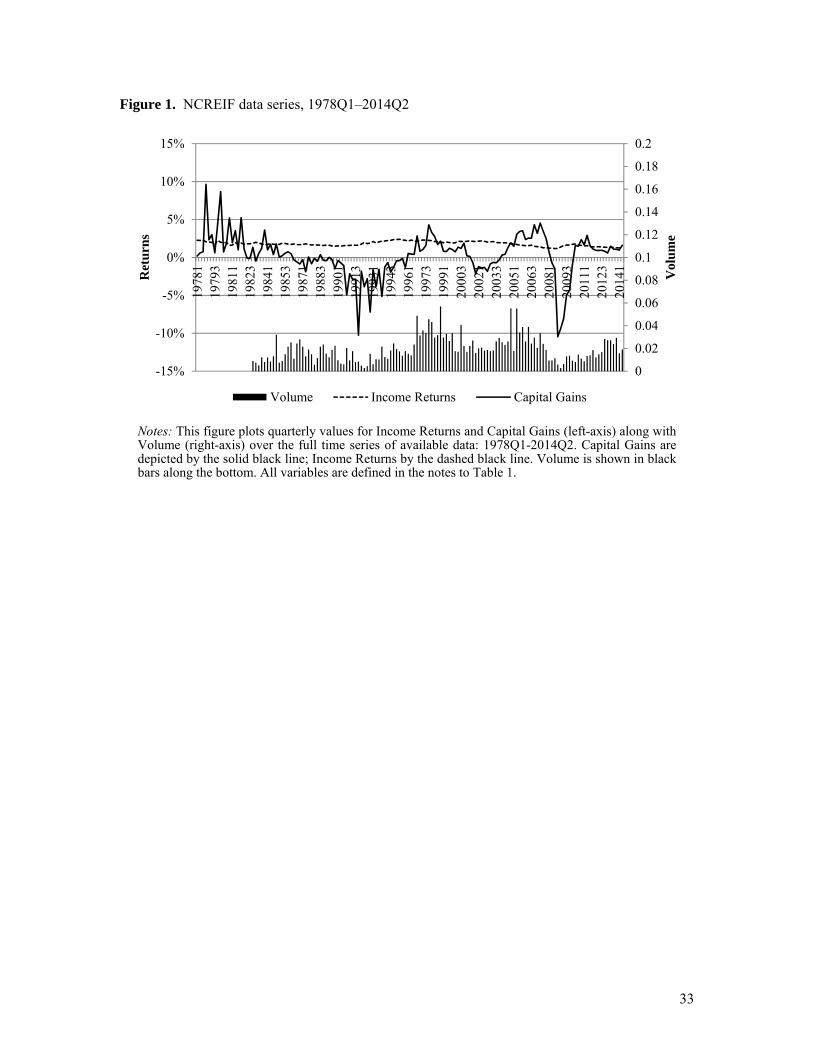
partitioned into Income Returns and Capital Gains components. Figure 1 displays the

time series. Income Returns are depicted by the dashed line; Capital Gains by the solid

bold line. Volume is measured as the percentage of turnover in the NCREIF database per

quarter based on the number of transactions in the TBI (Transactions-Based Index) which

initiates in 1982. The proxy for Volume using turnover in the NCREIF index was

developed by Fisher, Gatzlaff, Geltner and Haurin (2003) – it is the same measure as

used by Ling, Naranjo and Scheick (2014).

From Figure 1 it is apparent that Capital Gains returns are highly volatile while

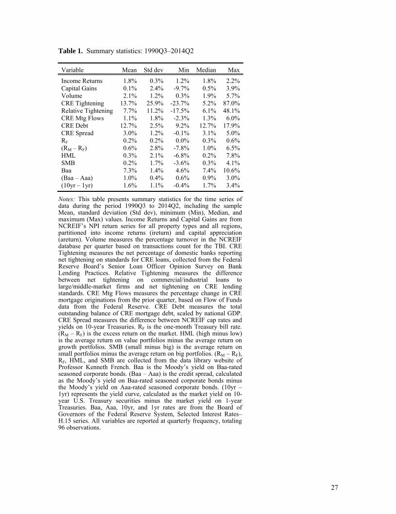
Income Returns are stable through CRE cycles. Table 1 presents summary statistics for

the 96 quarter sample period. Values for the NCREIF series include Income Returns,

Capital Gains, and Volume. Quarterly Income Returns average 1.8 percent with standard

deviation 0.3 percent. By comparison, the sample average for Capital Gains is 0.1 percent

12

with standard deviation 2.4 percent. Capital Gains are much more volatile than Income

Returns throughout the sample. The standard deviation of quarterly Capital Gains is 8

times greater than that of Income Returns, even while average Capital Gains are less than

1/18th the average value for Income Returns. Capital Gains and Income Returns series are

largely uncorrelated spanning multiple economic cycles (correlation coefficients is just

0.017 for the series). Anecdotally, the picture in Figure 1 suggests that cycles in CRE

prices are unlikely determined exclusively by cycles in the underlying property market

fundamentals. Thus, the role of capital market conditions in producing asset price

cyclicality for CRE is given careful consideration.

Capital markets include both debt and equity. The contribution of credit policy is

the central focus of this study. The variable of interest is CRE Tightening from the

Federal Reserve Board’s Senior Loan Officer Opinion Survey on Bank Lending

Practices. CRE Tightening measures the net percentage of domestic banks reporting net

tightening on standards for CRE loans. The CRE Tightening measure is reported at

quarterly frequency from 1990Q3 thru 2014Q2, which represents the sample period for

the analysis in this study [96 quarters]. Overall, banks are net tightening during the

sample. The average share of banks net tightening their lending standards in the CRE

sector is 13.7 percent. Yet, CRE lending policy is quite volatile and unsmooth with

standard deviation 25.9 percent; values range from 23.7 percent of banks net loosening to

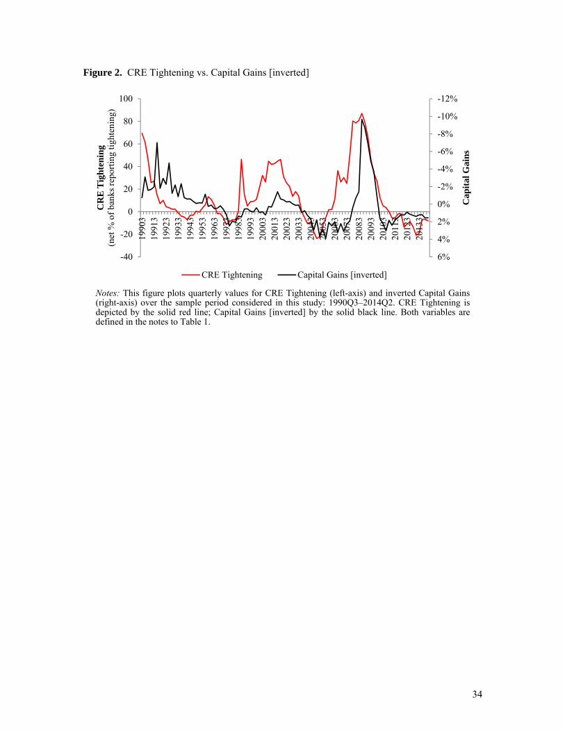
87 percent net tightening during the sample. Figure 2 shows the pattern in Credit

Tightening and inverted Capital Gains for the sample period. The two series move in

unison with CRE Tightening in the lead. Spikes in CRE Tightening are commonly

followed soon after by sharp declines in Capital Gains.

13

Wilcox (2012) comments that net tightening may not fully capture CRE

underwriting standards and develops his own underwriting index as an alternative

measure. In an attempt to address this concern, several other CRE mortgage condition

measures are considered including Relative Tightening, CRE Mtg Flows, CRE Debt, and

CRE Spread. Relative Tightening measures the difference between net tightening to on

commercial/industrial loans to large/middle-market firms and net tightening in CRE

lending standards. Relative Tightening attempts to isolate the component of changes in

bank lending policy that is CRE sector-specific. Lending policy is increasingly restrictive

relative to commercial loans during the sample, with average Relative Tightening at 7.7

percent for CRE lending over commercial loans.

Another possible issue with the CRE Tightening measure is that it is based on

survey responses and does not directly measure a quantity of loans approved in the CRE

market. CRE Mtg Flows provides such a measure, based on Flow of Funds data from the

Federal Reserve. CRE Mtg Flows measures the percentage change in CRE mortgage

originations from the prior quarter. Average CRE Mtg Flows are increasing 1.1 percent

per quarter, but rise by as much as 6 percent at the peak. Another direct measure for CRE

lending is total CRE Debt, which accounts for the total outstanding balance of CRE

mortgage debt – scaled by GDP. CRE Debt ranges from 9 percent to 18 percent of GDP

during the sample.

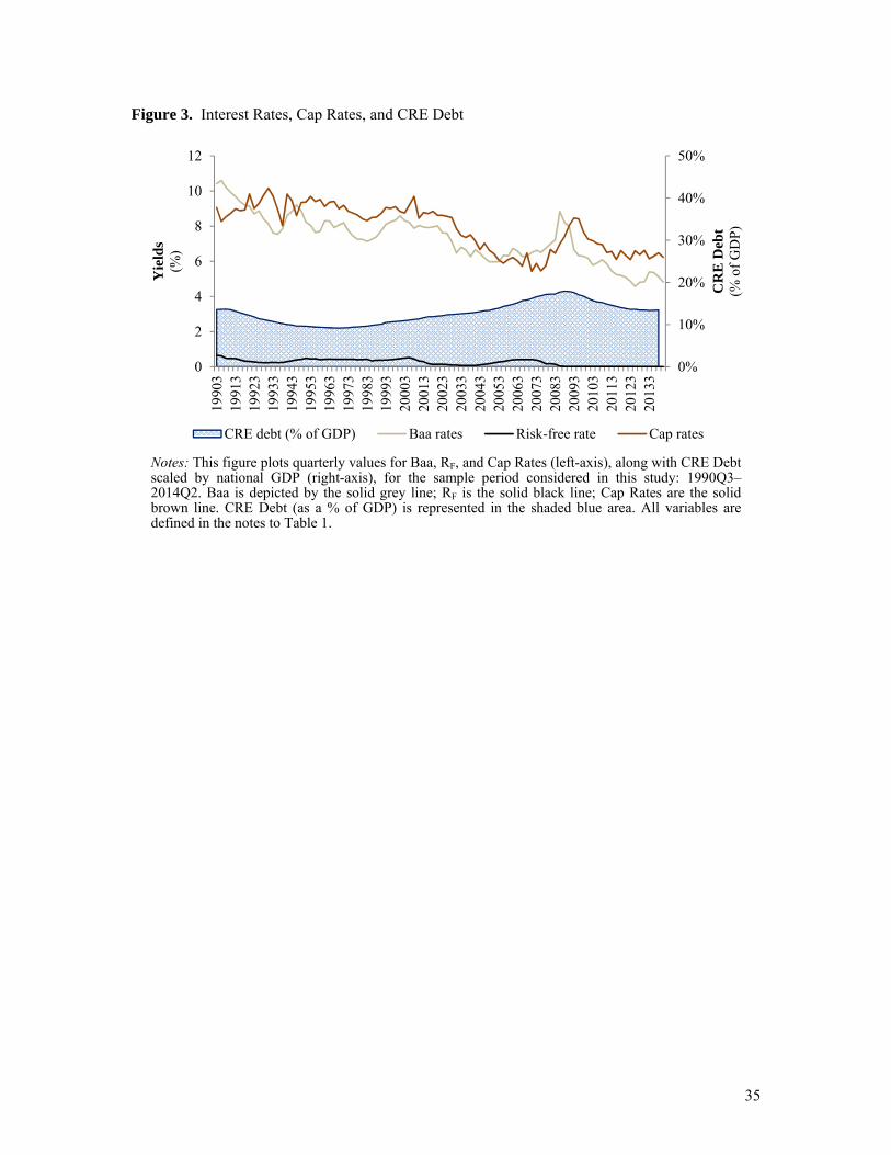
Mortgage pricing, or yields, are also relevant to asset prices (in addition to

mortgage quantities). CRE Spread measures the difference between NCREIF cap rates

and yields on 10-year Treasuries. The CRE Spread measure is included in the Cleveland

Financial Stress Index. During the sample period, the risk-free interest rate (RF) is very

14

low and experiences little volatility, while yields on Baa-rated bonds are more closely

related to CRE cap rates. The pattern is shown in Figure 3, along with CRE debt levels.

Accordingly, the Baa rate is used as the baseline yield in place of the risk-free rate in

estimations where exogenous factors are included. Otherwise, the set of exogenous

factors is largely consistent with that of Ling, Naranjo and Scheick (2014), including the

Fama-French three factors, collected from Professor French’s website: the market risk

premium (RM – RF), high-minus-low (HML), and small-minus-big (SMB); the credit

spread (Baa – Aaa), and the term structure (10yr – 1yr) from the Federal Reserve’s

Selected Interest Rates series. Apart from presentation of summary statistics in Table 1,

all variables are standardized with zero mean and unit standard deviation to limit issues

with comparing effects after modeling for variables that have different ranges or units of

measure.

The empirical approach considers that Income Returns, Capital Gains, Volume

(transactions), and Credit Tightening are mutually endogenous CRE variables. To

determine the appropriate methodology, the four variables are evaluated for issues that

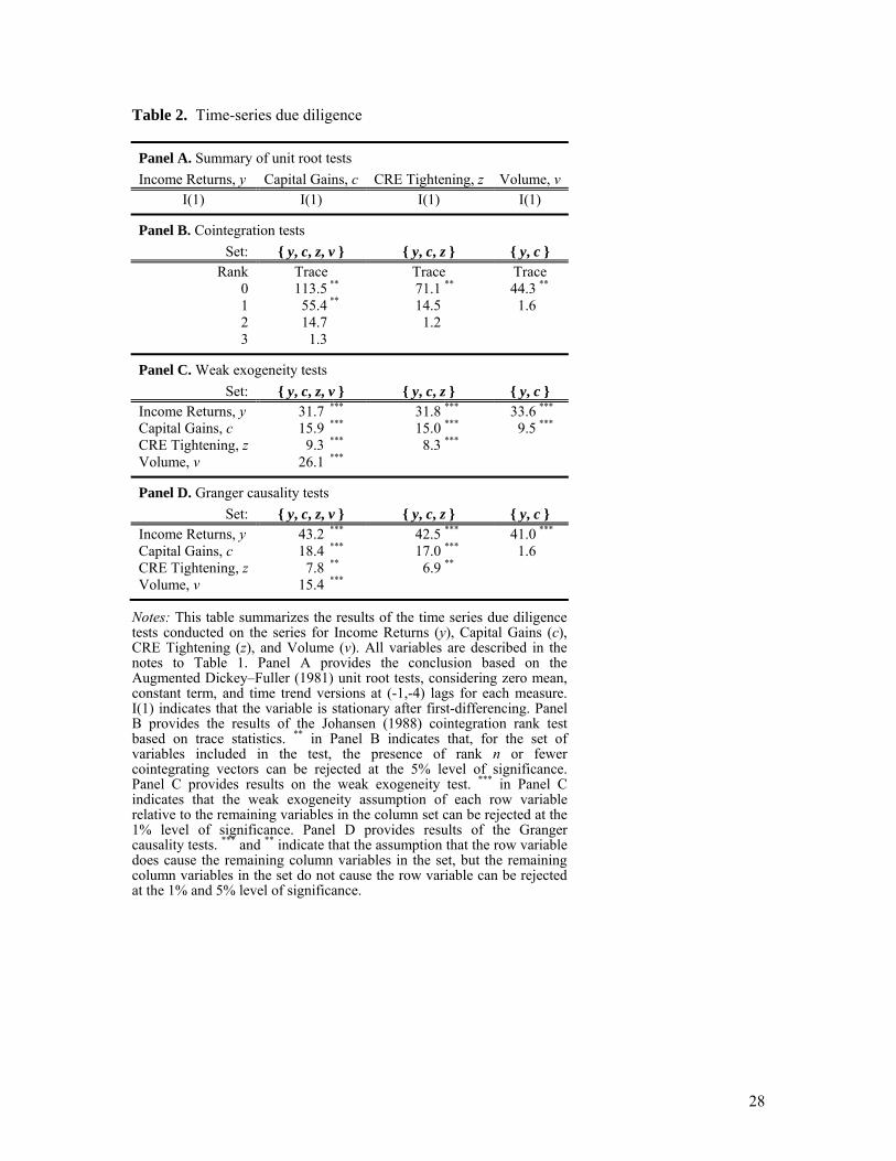
are prevalent in time series data. Results from the time series due diligence tests are

reported in Table 2. In Panel A, all four series are non-stationary. In Panel B, three

subsets of endogenous variables are tested for cointegration. The set {Income Returns,

Capital Gains, CRE Tightening, Volume} has two cointegrating vectors. The sets

{Income Returns, Capital Gains, CRE Tightening} and {Income Returns, Capital Gains}

each have a single cointegrating vector – suggesting that an error correction model may

be appropriate. In Panel C, all four variables are rejected for weak exogeneity when

tested against the various subsets of remaining variables. In Panel D, it can be rejected

15

that each of the four endogenous variables causes, while not being caused by, subsets of

the remaining variables with one exception: Income Returns do not cause Capital Gains

when considered in isolation.

In light of the time series due diligence, the empirical analysis considers three

models – with varying econometric tradeoffs involved. Each model considers variables

lagged one period, due to the quarterly nature of the data and to provide consistency in

model comparison. Two versions of each model are estimated: one includes endogenous

variables only; the second includes a set of six exogenous controls. The exogenous

controls are the Baa rate, (RM – RF), HML, SMB, (Baa – Aaa), and (10yr – 1yr).

The first model is the vector error correction model (VECM), evaluating Income

Returns, Capital Gains, and CRE Tightening as endogenous. When two or more variables

are non-stationary they may be cointegrated and share a common stochastic trend. The

two-stage VECM may be appropriate when there is only one cointegrating vector (as

evidenced for the set of variables in time series due diligence), leading to a single error

correction term. The VECM has the advantage of embedding short-run dynamics and

long-run equilibrium in two stages.

When there is evidence of more than one cointegrating vector, vector

autoregressive (VAR) modeling can be applied to capture the dynamic linkages among

the set of variables. VAR modeling does not require the same set of restrictions on

underlying parameters as VECM. Ordering of endogenous variables in the VAR system

of equations may affect the empirical outcome. In this study, the effects in a given quarter

are assumed to hold the following sequential order: Income Returns, Credit Tightening,

Volume, Capital Gains. Income Returns from the property market are observed first.

16

Credit Tightening can then be adjusted based on information about the property market

fundamentals. Quarterly transaction Volume is affected by the degree of Credit

Tightening. Finally, Capital Gains are realized as a consequence of all of the above,

including shifts in Income Returns making asset yields more or less attractive, Credit

Tightening impacting levered returns and Volume, then Volume directly affecting Capital

Gains due to the highly illiquid nature of CRE transactions markets. Ultimately, the

empirical results using the series of data in this study are robust to alternative ordering

selections.

This study presents two sets of results for each VECM and VAR model. The first

set of results includes all endogenous variables, along with six exogenous variables that

are used to condition the endogenous measures for other potential sources of variation

responding to macroeconomic conditions. The first set of results is provided for

comparison to related work in the extant literature. The second set of results includes

only endogenous variables (i.e., does not include exogenous factors). The advantage of

the second approach is in the opportunity to quantify the variance decomposition when

only endogenous variables are included. To produce the impulse response functions (IRF)

and variance decompositions, the Choleski decomposition is used, which models the

error term matrix as a recursive triangular system. The number of lags is selected based

on AIC criteria. AIC values are highly similar in models with one, two or three lags.

However, none of the endogenous or exogenous variables appear significant beyond the

first lag, thus VAR/VECM(1,1) and VAR/VECM(1) models are reported in this study,

while higher lag options produce qualitatively similar results.

17

IV. Results

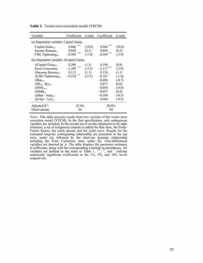
Results from the VECM estimations are presented in Table 3. In the first-stage, the long-

run equilibrium relation between Capital Gains, Income Returns, and CRE Tightening is

estimated. The coefficients are 0.666 for Capital Gains and -0.269 for CRE Tightening,

whereas Income Returns has no significant effect on Capital Gains in the long-run.

Capital Gains are highly sensitive to CRE Tightening. When deviations in Capital Gains

from its mean coincide with deviations in CRE Tightening that are 2.5 times greater,

there is no need for error correction and the two variables are in long-run equilibrium.

Thus, there is an optimal responsiveness of credit policy to CRE price growth.

The error term from the first-stage of the VECM is collected and included in the

second-stage for first-differences – considering short-run dynamics. Increases in CRE

Tightening create distortions in CRE asset prices causing Capital Gains to be too high

relative to long-run equilibrium. From the Error Correction coefficient, no less than 100

percent of any such deviation in Capital Gains from long-run equilibrium will be

corrected in the subsequent quarter. A one standard deviation increase in CRE Tightening

(26 percent of banks net tightening to CRE sector) immediately causes a 0.21 standard

deviation reduction in Capital Gains (50 basis points, which is 5 times greater than the

mean value) in the following quarter. Income Returns have zero impact on Capital Gains

in both the short-run and long-run. Surprisingly, upon introducing the Error Correction

term, lagged changes in Capital Gains have no immediate effect on current realized

values. Neither do any of the exogenous factors considered. In the immediate horizon, the

only distortions in Capital Gains are in response to CRE Tightening along with an Error

Correction term that quickly returns the two series to their long-run equilibrium state.

18

Results from the estimation of the VAR system that includes four equations

(VAR:4) with four endogenous variables and six exogenous variables are presented in

Table 4. Income Returns are positively related to prior values, but inversely related to

Capital Gains. Following periods of capital appreciation, asset prices are bid upward

relative to income, lowering yields. CRE Tightening replicates its own past behavior and

is also inversely related to macroeconomic factors including the market risk premium and

SMB. When yields on risky assets rise relative to the risk-free rate, credit is loosened in

the following period. Transactions Volume is positively related to Income Returns,

Capital Gains, and recent Volume, but responds negatively to CRE Tightening –

consistent with expectations.

In the far-right columns of Table 4, evidence for the long-run equilibrium

relationship between Capital Gains and CRE Tightening is largely consistent with results

from the VECM estimations. Capital Gains are positively related to their past realized

value. Positive Capital Gains create higher valuations that are followed by subsequently

higher valuations. Periods of asset sell-offs and dropping values are also sequential. An

increase in CRE Tightening clamps down on the Capital Gains trajectory.

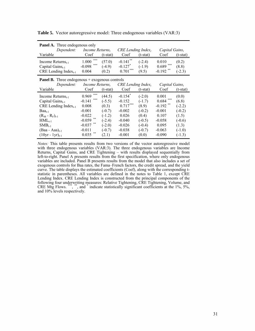
Table 5 presents results for the specification that includes only three endogenous

factors (VAR:3): Income Returns, Capital Gains, and a CRE Lending Index constructed

from the principal components of four underwriting measures. The four underwriting

measures are Relative Tightening, CRE Tightening, Volume, and the percentage change

in CRE Mtg Flows. These four measures are identified as the most informative

underwriting measures, based on factor analysis for a set of measures that also included

CRE Debt and CRE Spread. Applying the CRE Lending Index produces highly similar

19

results to the CRE Tightening measure. In the Capital Gains estimation, coefficients for

lagged Capital Gains are 0.689 and 0.684 (compared with coefficients of 0.623 and 0.680

in Table 4), while the coefficient for the CRE Lending Index is -0.192 (compared to

values of -0.268 and -0.273 for CRE Tightening in Table 4). Once again, suppressing

exogenous factors in the estimation produces similar results. Periods of high income

returns are preceded by periods of high income returns. It suggests that changes in the

underlying property market fundamentals are sustained over a long horizon, such as

improvements in the sector occupancy rates or effective rents.

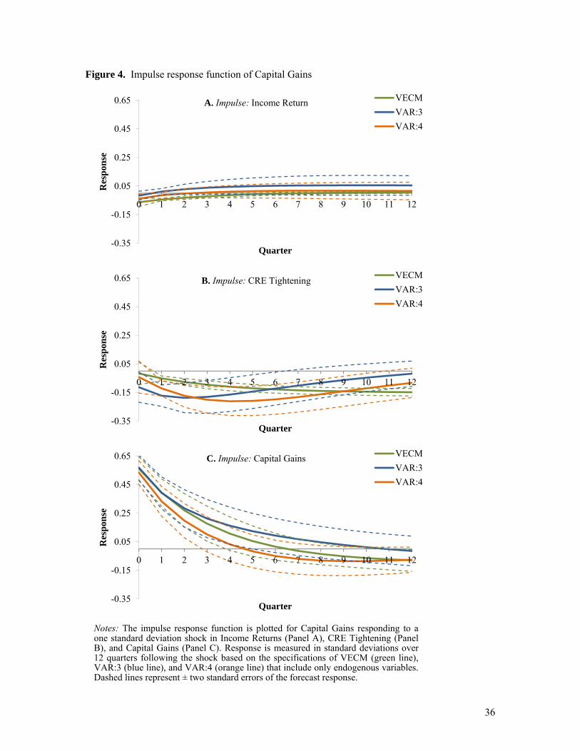
Figure 4 illustrates the response function for Capital Gains following the

orthogonalized impulses of Income Returns (in Panel A), CRE Tightening (in Panel B),

and Capital Gains (in Panel C). A one standard deviation shock to Income Returns has

essentially zero impact on Capital Gains – even up to three years after. In all three

models, a one standard deviation shock to CRE Tightening (Panel B) has a negative and

significant impact on Capital Gains, pulling down asset prices by -0.1 to -0.2 standard

deviations (24 to 48 basis points per quarter) over an extended horizon. In Panel C,

increases in Capital Gains in a given period are positively related to the prior period

increase. Apart from its own past realized value, Capital Gains are not determined by

yields in the underlying property market (i.e., Income Returns). Instead, changes in CRE

Tightening plays the central role in affecting Capital Gains outcomes – with lasting

effects.

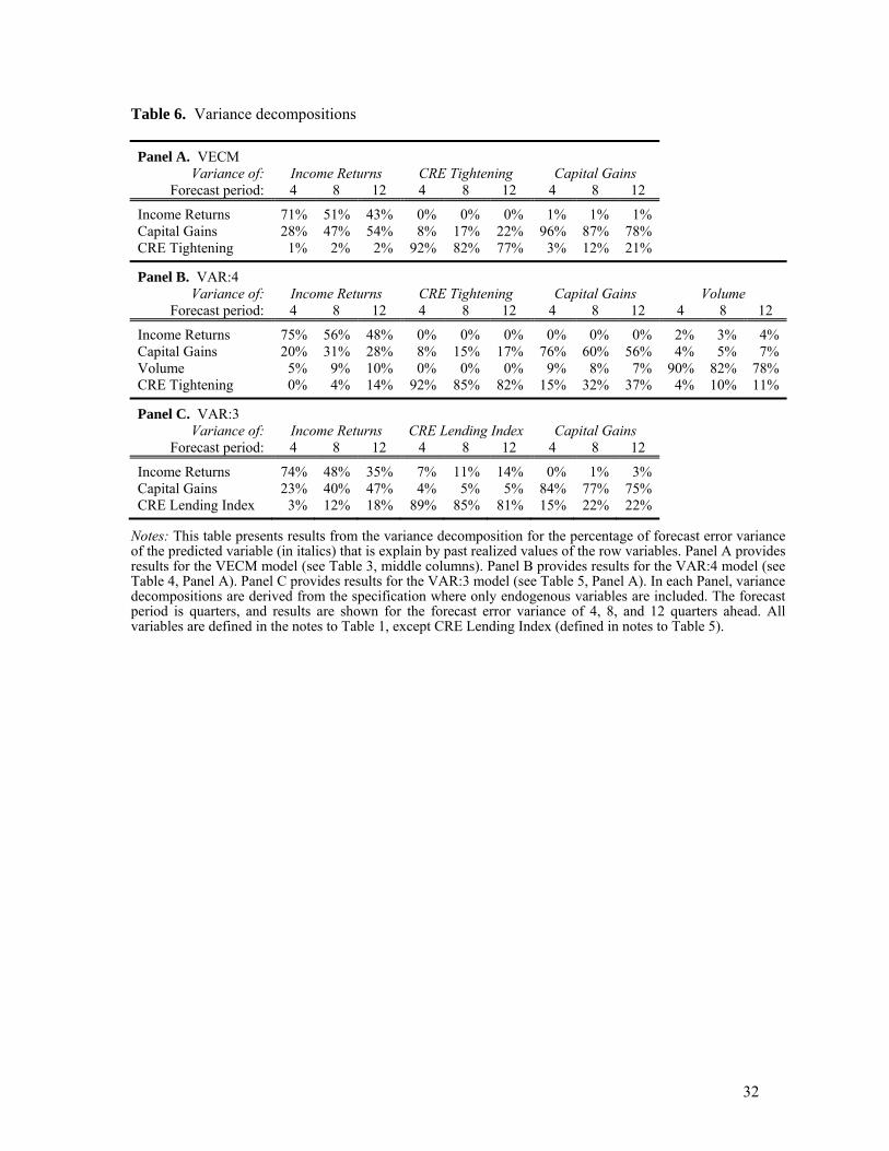
The fully endogenous VAR and VECM specifications enable variance

decompositions. Table 6 reports the 4, 8, and 12 quarter lead prediction errors that are

explained by each endogenous measure. Volatility in Income Returns is explained largely

20

by its own variance and also by volatility in Capital Gains. Over a one- to three-year

horizon, 28 to 54 percent of the variance in Income Returns is explained by fluctuations

in Capital Gains. By comparison, volatility in CRE Tightening is predominantly

explained by its own preceding realized value. No less than 77 percent of the prediction

error for CRE Tightening is explained by past volatility in CRE Tightening. This result

suggests that CRE Tightening is largely decided at a macroeconomic and policy level,

rather than as responsive to changes in the asset market itself. For Capital Gains,

volatility in CRE Tightening has long-lasting effects. Up to 37 percent of the variance in

Capital Gains is explained by changes in credit policy over a subsequent 12 quarter

period.

V. Conclusions

Conventional wisdom suggests that asset prices should respond to income yields and

should exhibit some sensitivity to transaction volume in a highly illiquid market, such as

CRE. Evidence provided in this study fails to support either of these assertions. Capital

gains in CRE are largely unresponsive to changes in income returns and transaction

volume. Instead, the illiquid nature of the asset market perpetuates periods of

autocorrelation in capital gains, creating an inefficient market characterized by slow and

prolonged pricing cycles. Apart from return-chasing behavior, the dominant factor

affecting CRE pricing cycles is credit policy, accounting for up to 37 percent of the

prediction error in capital gains. Credit tightening itself is largely unrelated to CRE

fundamentals.

21

Looseness or tightness in credit policy can be transmitted to CRE asset prices in a

number of ways. However, considering evidence that CRE price volatility is affected by

credit policy and not transaction volume suggests that these price effects are not caused

by the liquidity channel. Instead, shifts in credit policy directly affect levered returns for

assets sold in a given period, enabling investors to lever up or lever down their valuations

on assets available for purchase. Thus, credit policy transmission to CRE prices occurs

through the valuation channel rather than the liquidity channel as previously believed.

The results of this study suggest that a more stabilized and consistent credit policy is

likely to significantly reduce the magnitude of fluctuations in CRE pricing spirals.

22

Appendix. Alternate Specifications & Data

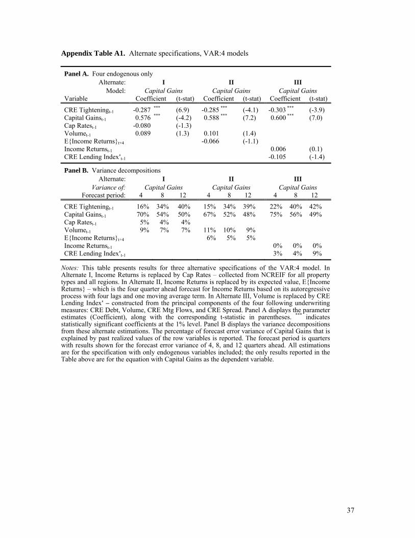
For robustness, a few alternative specifications are considered. One concern is that the

Income Returns measure does not directly measure yields, or at least in the way that CRE

investors are applying yields for investment purpose. Alternate I considers using Cap

Rates as a substitute for Income Returns, which offers a linkage to property market

effects that is more aligned with the framework of Ghysels, Plazzi, Torous and Valkanov

(2012). Cap Rates are collected from NCREIF for all property types and all regions. A

second concern is that investors may be primarily concerned with forward-looking

expected values for income returns (rather than past values). Alternate II provides a

specification where the lagged Income Returns measure is replaced by its four quarter

forward expected value, generated from an autoregressive process. A third concern is that

the CRE Lending Index measure is dominated by the CRE Tightening measure, so it may

be revealing to see an alternative lending index. In Alternate III, Volume is replaced by

CRE Lending Index' – constructed from the principal components of the four following

underwriting measures: CRE Debt, Volume, CRE Mtg Flows, and CRE Spread.

Interestingly, CRE Lending Index' is largely uncorrelated with CRE Tightening. Results

for Alternate specifications I, II, and III are provided in Table A1. The central result is

largely unchanged under the alternate specifications. Capital Gains respond positively to

recent changes in Capital Gains and negative to recent changes in CRE Tightening.

Credit policy accounts for a large portion of the forecast error for Capital Gains, while

influence from the property market is close to zero.

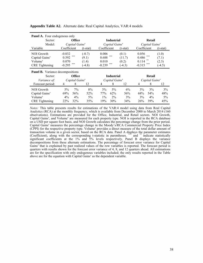
An alternate to the NCREIF series is Real Capital Analytics (RCA), available at

monthly frequency beginning in December 2000. RCA data has 160 monthly

23

observations compared to 96 quarterly observations for NCREIF, although the series

spans fewer cycles. An issue with Income Returns is that asset values are implicitly in the

denominator, even if unobserved for several periods, leading to potentially abrupt

changes when asset valuations are adjusted. Income reporting may be smoothed over

calendar quarters for accounting purposes. Thus, Income Returns do not provide as direct

a measure for property market fundamentals as NOI on per square foot basis might,

which is available in the RCA data. Another concern is whether NCREIF turnover is the

most meaningful proxy for aggregate transaction volume since assets comprising the TBI

represent a relatively small percentage of total CRE assets and they are held by tax-

exempt institutional investor clienteles (primarily pension funds). A direct measure for

transaction volume based on the total dollar amount of CRE sold is available in the RCA

data. Finally, the Moody’s/RCA Commercial Property Price Index (CPPI) is a constant-

quality index and is not appraisal based, which circumvents issues with TBI and NCREIF

NPI measures for Capital Gains. Results from estimations by property type using the

RCA data are presented in Table A2. The central findings of this study are robust to the

alternate data source.

24

References

Amihud, Y., Mendelson, H., Pedersen, L.H. (2005). Liquidity and Asset Prices.

Foundations and Trends in Finance, 1:269–364.

Arsenault, M., Clayton, J., Peng, L. (2013). Mortgage Fund Flows, Capital Appreciation,

and Real Estate Cycles. Journal of Real Estate Finance and Economics, 47:243–265.

Carhart, M.M. (1997). On Persistence in Mutual Fund Performance. Journal of Finance,

52:57–82.

Chen, G., Firth, M., Rui, O. (2001). The Dynamic Relation between Stock Returns,

Trading Volume and Volatility. The Financial Review, 38:153–174.

Chuang, C.C., Kuan, C.M., Lin, H.Y. (2009). Causality in Quantiles and Dynamic Stock

Return-Volume Relations. Journal of Banking and Finance, 33:1351–1360.

Clayton, J. (2009). Debt Matters: Leverage, Liquidity, and Property Valuation. Journal of

Real Estate Portfolio Management, 15:107–113.

Clayton, J., MacKinnon, G., Peng, L. (2005). Time Variation of Liquidity in the Private

Real Estate Market: Causes and Consequences. RERI Grant / working paper.

Dickey, D., Fuller, W.A. (1981). Likelihood Ratio Statistics for Autoregressive Time

Series with a Unit Root. Econometrica, 49:1057–1072.

Fisher, J., Gatzlaff, D., Geltner, D., Haurin, D. (2003). Controlling for the Impact of

Variable Liquidity in Commercial Real Estate Price Indices. Real Estate Economics,

31:269–303.

Friesen, G.C., Sapp, T.R.A. (2007). Mutual Fund Flows and Investor Returns: An

Empirical Examination of Fund Investor Timing Ability. Journal of Banking and

Finance, 31:2796–2816.

Geltner, D., Pollakowski, H. (2007). A Set of Indexes for Trading Commercial Real

Estate Based on the Real Capital Analytics Transaction Prices Database,

MIT/CREDL.

Gervais, S., Kaniel, R., Mingelgrin, D. (2001). The High Volume Return Premium.

Journal of Finance, 56:877–919.

25

Ghysels, E., Plazzi, A., Valkanov, R. (2007). Valuation in US Commercial Real Estate.

European Financial Management, 13:472–497.

Ghysels, E., Plazzi, A., Torous, W., Valkanov, R. (2012). Forecasting Real Estate Prices.

In Handbook of Economic Forecasting.

Grovenstein, R.A., Harding, J.P., Sirmans, C.F., Thebpanya, S., Turnbull, G.K. (2005).

Commercial Mortgage Underwriting: How Well Do Lenders Manage the Risks?

Journal of Housing Economics, 14:355–383.

Jorgenson, D. (1960). A Dual Stability Theorem. Econometrica, 28:892–999.

Johansen, S. (1988). Statistical Analysis of Cointegration Vectors. Journal of Economics

Dynamics and Control, 12:231–254.

Kaniel, R., Ozoguz, A., Starks, L. (2012). The High Volume Return Premium: Cross-

country Evidence. Journal of Financial Economics, 103:255–279.

Karpoff, J.M. (1987). The Relation between Price Changes and Trading Volume: A

Survey. Journal of Financial and Quantitative Analysis, 22:109–126.

Lee, T.H., Rui, O. (2002). The Dynamic Relationship between Stock Return and Trading

Volume: Domestic and Cross-country Evidence. Journal of Banking and Finance,

26:51–78.

Ling, D.C., Marcato, G., McAllister, P. (2009). Dynamics of Asset Prices and

Transaction Activity in Illiquid Markets: the Case of Private Commercial Real Estate.

Journal of Real Estate Finance and Economics, 39:359–383.

Ling, D.C., Naranjo, A., Scheick, B. (2014). Credit Availability and Asset Pricing

Dynamics in Illiquid Markets: Evidence from Commercial Real Estate Markets. RERI

Grant / working paper.

MacKinnon, G.H., Al-Zaman, A. (2009). Real Estate for the Long Term: The Effect of

Return Predictability on Long-Horizon Allocations. Real Estate Economics, 37:117–

153.

Plazzi, A., Torous, W., Valkanov, R. (2011). Exploiting Property Characteristics in

Commercial Real Estate Portfolio Allocation. Journal of Portfolio Management,

35:39–50.

26

Wilcox, J. (2012). Commercial Real Estate: Underwriting, Mortgages, and Prices. RERI

Grant / working paper.

27

Table 1. Summary statistics: 1990Q3–2014Q2

Variable Mean Std dev Min Median Max

Income Returns 1.8% 0.3% 1.2% 1.8% 2.2% Capital Gains 0.1% 2.4% -9.7% 0.5% 3.9% Volume 2.1% 1.2% 0.3% 1.9% 5.7% CRE Tightening 13.7% 25.9% -23.7% 5.2% 87.0% Relative Tightening 7.7% 11.2% -17.5% 6.1% 48.1% CRE Mtg Flows 1.1% 1.8% -2.3% 1.3% 6.0% CRE Debt 12.7% 2.5% 9.2% 12.7% 17.9% CRE Spread 3.0% 1.2% -0.1% 3.1% 5.0% RF 0.2% 0.2% 0.0% 0.3% 0.6% (RM – RF) 0.6% 2.8% -7.8% 1.0% 6.5% HML 0.3% 2.1% -6.8% 0.2% 7.8% SMB 0.2% 1.7% -3.6% 0.3% 4.1% Baa 7.3% 1.4% 4.6% 7.4% 10.6% (Baa – Aaa) 1.0% 0.4% 0.6% 0.9% 3.0% (10yr – 1yr) 1.6% 1.1% -0.4% 1.7% 3.4%

Notes: This table presents summary statistics for the time series of data during the period 1990Q3 to 2014Q2, including the sample Mean, standard deviation (Std dev), minimum (Min), Median, and maximum (Max) values. Income Returns and Capital Gains are from NCREIF’s NPI return series for all property types and all regions, partitioned into income returns (ireturn) and capital appreciation (areturn). Volume measures the percentage turnover in the NCREIF database per quarter based on transactions count for the TBI. CRE Tightening measures the net percentage of domestic banks reporting net tightening on standards for CRE loans, collected from the Federal Reserve Board’s Senior Loan Officer Opinion Survey on Bank Lending Practices. Relative Tightening measures the difference between net tightening on commercial/industrial loans to large/middle-market firms and net tightening on CRE lending standards. CRE Mtg Flows measures the percentage change in CRE mortgage originations from the prior quarter, based on Flow of Funds data from the Federal Reserve. CRE Debt measures the total outstanding balance of CRE mortgage debt, scaled by national GDP. CRE Spread measures the difference between NCREIF cap rates and yields on 10-year Treasuries. RF is the one-month Treasury bill rate. (RM – RF) is the excess return on the market. HML (high minus low) is the average return on value portfolios minus the average return on growth portfolios. SMB (small minus big) is the average return on small portfolios minus the average return on big portfolios. (RM – RF), RF, HML, and SMB are collected from the data library website of Professor Kenneth French. Baa is the Moody’s yield on Baa-rated seasoned corporate bonds. (Baa – Aaa) is the credit spread, calculated as the Moody’s yield on Baa-rated seasoned corporate bonds minus the Moody’s yield on Aaa-rated seasoned corporate bonds. (10yr – 1yr) represents the yield curve, calculated as the market yield on 10-year U.S. Treasury securities minus the market yield on 1-year Treasuries. Baa, Aaa, 10yr, and 1yr rates are from the Board of Governors of the Federal Reserve System, Selected Interest Rates–H.15 series. All variables are reported at quarterly frequency, totaling 96 observations.

28

Table 2. Time-series due diligence

Panel A. Summary of unit root tests

Income Returns, y Capital Gains, c CRE Tightening, z Volume, v I(1) I(1) I(1) I(1)

Panel B. Cointegration tests

Set: { y, c, z, v } { y, c, z } { y, c } Rank Trace Trace Trace

0 113.5 ** 71.1 ** 44.3 ** 1 55.4 ** 14.5 1.62 14.7 1.23 1.3

Panel C. Weak exogeneity tests

Set: { y, c, z, v } { y, c, z } { y, c } Income Returns, y 31.7 *** 31.8 *** 33.6 *** Capital Gains, c 15.9 *** 15.0 *** 9.5 *** CRE Tightening, z 9.3 *** 8.3 *** Volume, v 26.1 ***

Panel D. Granger causality tests

Set: { y, c, z, v } { y, c, z } { y, c } Income Returns, y 43.2 *** 42.5 *** 41.0 *** Capital Gains, c 18.4 *** 17.0 *** 1.6CRE Tightening, z 7.8 ** 6.9 ** Volume, v 15.4 ***

Notes: This table summarizes the results of the time series due diligence tests conducted on the series for Income Returns (y), Capital Gains (c), CRE Tightening (z), and Volume (v). All variables are described in the notes to Table 1. Panel A provides the conclusion based on the Augmented Dickey–Fuller (1981) unit root tests, considering zero mean, constant term, and time trend versions at (-1,-4) lags for each measure. I(1) indicates that the variable is stationary after first-differencing. Panel B provides the results of the Johansen (1988) cointegration rank test based on trace statistics. ** in Panel B indicates that, for the set of variables included in the test, the presence of rank n or fewer cointegrating vectors can be rejected at the 5% level of significance. Panel C provides results on the weak exogeneity test. *** in Panel C indicates that the weak exogeneity assumption of each row variable relative to the remaining variables in the column set can be rejected at the 1% level of significance. Panel D provides results of the Granger causality tests. *** and ** indicate that the assumption that the row variable does cause the remaining column variables in the set, but the remaining column variables in the set do not cause the row variable can be rejected at the 1% and 5% level of significance.

29

Table 3. Vector error correction model (VECM)

Variable Coefficient (t-stat) Coefficient (t-stat)

(a) Dependent variable: Capital Gainst         

Capital Gainst-1 0.666 *** (10.0) 0.666 *** (10.0) Income Returnst-1 0.020 (0.3) 0.020 (0.3) CRE Tighteningt-1 -0.269 *** (-3.9) -0.269 *** (-3.9)

(b) Dependent variable: ΔCapital Gainst        

ΔCapital Gainst-1 0.296 (1.5) 0.190 (0.8) Error Correctiont -1.209 *** (-3.3) -1.117 *** (-2.9) ΔIncome Returnst-1 0.113 (1.1) 0.120 (1.1) ΔCRE Tighteningt-1 -0.210 ** (-2.3) -0.181 * (-1.8) ΔBaat-1 -0.084 (-0.7) Δ(RM - RF)t-1 0.071 (0.6) ΔHMLt-1 -0.054 (-0.8) ΔSMBt-1 -0.057 (0.4) Δ(Baa - Aaa)t-1 -0.109 (-0.5) Δ(10yr - 1yr)t-1 0.044 (-0.5)

Adjusted R2: 23.4% 20.9% Observations: 94 94

Notes: This table presents results from two versions of the vector error correction model (VECM). In the first specification, only endogenous variables are included. In the second set of results (displayed in far-right columns), a set of exogenous controls is added for Baa rates, the Fama-French factors, the credit spread, and the yield curve. Results for the estimated long-run cointegrating relationship are presented in the top rows, under (a), followed by the short-run dynamic relationship including the Error Correction term, under (b). First-differenced variables are denoted by Δ. The table displays the parameter estimates (Coefficient), along with the corresponding t-statistic in parentheses. All variables are defined in the notes to Table 1. ***, **, and * indicate statistically significant coefficients at the 1%, 5%, and 10% levels respectively.

30

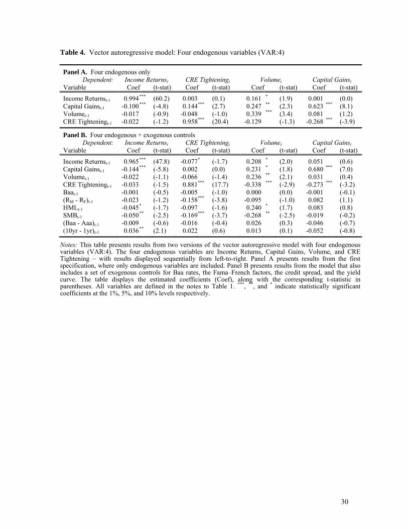
Table 4. Vector autoregressive model: Four endogenous variables (VAR:4)

Panel A. Four endogenous only Dependent: Income Returnst CRE Tighteningt Volumet Capital Gainst

Variable Coef (t-stat) Coef (t-stat) Coef (t-stat) Coef (t-stat)

Income Returnst-1 0.994 *** (60.2) 0.003 (0.1) 0.161 * (1.9) 0.001 (0.0) Capital Gainst-1 -0.100 *** (-4.8) 0.144*** (2.7) 0.247 ** (2.3) 0.623 *** (8.1) Volumet-1 -0.017 (-0.9) -0.048 (-1.0) 0.339 *** (3.4) 0.081 (1.2) CRE Tighteningt-1 -0.022 (-1.2) 0.958*** (20.4) -0.129 (-1.3) -0.268 *** (-3.9)

Panel B. Four endogenous + exogenous controls Dependent: Income Returnst CRE Tighteningt Volumet Capital Gainst

Variable Coef (t-stat) Coef (t-stat) Coef (t-stat) Coef (t-stat)

Income Returnst-1 0.965 *** (47.8) -0.077* (-1.7) 0.208 * (2.0) 0.051 (0.6) Capital Gainst-1 -0.144 *** (-5.8) 0.002 (0.0) 0.231 * (1.8) 0.680 *** (7.0) Volumet-1 -0.022 (-1.1) -0.066 (-1.4) 0.236 ** (2.1) 0.031 (0.4) CRE Tighteningt-1 -0.033 (-1.5) 0.881*** (17.7) -0.338 *** (-2.9) -0.273 *** (-3.2) Baat-1 -0.001 (-0.5) -0.005 (-1.0) 0.000 (0.0) -0.001 (-0.1) (RM - RF)t-1 -0.023 (-1.2) -0.158*** (-3.8) -0.095 (-1.0) 0.082 (1.1) HMLt-1 -0.045 * (-1.7) -0.097 (-1.6) 0.240 * (1.7) 0.083 (0.8) SMBt-1 -0.050 ** (-2.5) -0.169*** (-3.7) -0.268 ** (-2.5) -0.019 (-0.2) (Baa - Aaa)t-1 -0.009 (-0.6) -0.016 (-0.4) 0.026 (0.3) -0.046 (-0.7) (10yr - 1yr)t-1 0.036 ** (2.1) 0.022 (0.6) 0.013 (0.1) -0.052 (-0.8)

Notes: This table presents results from two versions of the vector autoregressive model with four endogenous variables (VAR:4). The four endogenous variables are Income Returns, Capital Gains, Volume, and CRE Tightening – with results displayed sequentially from left-to-right. Panel A presents results from the first specification, where only endogenous variables are included. Panel B presents results from the model that also includes a set of exogenous controls for Baa rates, the Fama–French factors, the credit spread, and the yield curve. The table displays the estimated coefficients (Coef), along with the corresponding t-statistic in parentheses. All variables are defined in the notes to Table 1. ***, **, and * indicate statistically significant coefficients at the 1%, 5%, and 10% levels respectively.

31

Table 5. Vector autoregressive model: Three endogenous variables (VAR:3)

Panel A. Three endogenous only Dependent: Income Returnst CRE Lending Indext Capital Gainst

Variable Coef (t-stat) Coef (t-stat) Coef (t-stat)

Income Returnst-1 1.000 *** (57.0) -0.141** (-2.4) 0.010 (0.2) Capital Gainst-1 -0.098 *** (-4.9) -0.127* (-1.9) 0.689 *** (8.8) CRE Lending Indext-1 0.004 (0.2) 0.701*** (9.5) -0.192 ** (-2.3)

Panel B. Three endogenous + exogenous controls Dependent: Income Returnst CRE Lending Indext Capital Gainst

Variable Coef (t-stat) Coef (t-stat) Coef (t-stat)

Income Returnst-1 0.969 *** (44.5) -0.154* (-2.0) 0.001 (0.0) Capital Gainst-1 -0.141 *** (-5.5) -0.152 (-1.7) 0.684 *** (6.8) CRE Lending Indext-1 0.008 (0.3) 0.717*** (8.9) -0.192 ** (-2.2) Baat-1 -0.001 (-0.7) -0.002 (-0.2) -0.001 (-0.2) (RM - RF)t-1 -0.022 (-1.2) 0.026 (0.4) 0.107 (1.5) HMLt-1 -0.059 ** (-2.4) -0.040 (-0.5) -0.058 (-0.6) SMBt-1 -0.037 ** (-2.0) -0.026 (-0.4) 0.095 (1.3) (Baa - Aaa)t-1 -0.011 (-0.7) -0.038 (-0.7) -0.063 (-1.0) (10yr - 1yr)t-1 0.035 ** (2.1) -0.001 (0.0) -0.090 (-1.3)

Notes: This table presents results from two versions of the vector autoregressive model with three endogenous variables (VAR:3). The three endogenous variables are Income Returns, Capital Gains, and CRE Tightening – with results displayed sequentially from left-to-right. Panel A presents results from the first specification, where only endogenous variables are included. Panel B presents results from the model that also includes a set of exogenous controls for Baa rates, the Fama–French factors, the credit spread, and the yield curve. The table displays the estimated coefficients (Coef), along with the corresponding t-statistic in parentheses. All variables are defined in the notes to Table 1, except CRE Lending Index. CRE Lending Index is constructed from the principal components of the following four underwriting measures: Relative Tightening, CRE Tightening, Volume, and CRE Mtg Flows. ***, **, and * indicate statistically significant coefficients at the 1%, 5%, and 10% levels respectively.

32

Table 6. Variance decompositions

Panel A. VECM Variance of: Income Returns CRE Tightening Capital Gains

Forecast period: 4 8 12 4 8 12 4 8 12

Income Returns 71% 51% 43% 0% 0% 0% 1% 1% 1% Capital Gains 28% 47% 54% 8% 17% 22% 96% 87% 78% CRE Tightening 1% 2% 2% 92% 82% 77% 3% 12% 21%

Panel B. VAR:4 Variance of: Income Returns CRE Tightening Capital Gains Volume

Forecast period: 4 8 12 4 8 12 4 8 12 4 8 12

Income Returns 75% 56% 48% 0% 0% 0% 0% 0% 0% 2% 3% 4% Capital Gains 20% 31% 28% 8% 15% 17% 76% 60% 56% 4% 5% 7% Volume 5% 9% 10% 0% 0% 0% 9% 8% 7% 90% 82% 78% CRE Tightening 0% 4% 14% 92% 85% 82% 15% 32% 37% 4% 10% 11%

Panel C. VAR:3 Variance of: Income Returns CRE Lending Index Capital Gains

Forecast period: 4 8 12 4 8 12 4 8 12

Income Returns 74% 48% 35% 7% 11% 14% 0% 1% 3% Capital Gains 23% 40% 47% 4% 5% 5% 84% 77% 75% CRE Lending Index 3% 12% 18% 89% 85% 81% 15% 22% 22%

Notes: This table presents results from the variance decomposition for the percentage of forecast error variance of the predicted variable (in italics) that is explain by past realized values of the row variables. Panel A provides results for the VECM model (see Table 3, middle columns). Panel B provides results for the VAR:4 model (see Table 4, Panel A). Panel C provides results for the VAR:3 model (see Table 5, Panel A). In each Panel, variance decompositions are derived from the specification where only endogenous variables are included. The forecast period is quarters, and results are shown for the forecast error variance of 4, 8, and 12 quarters ahead. All variables are defined in the notes to Table 1, except CRE Lending Index (defined in notes to Table 5).

33

Figure 1. NCREIF data series, 1978Q1–2014Q2

Notes: This figure plots quarterly values for Income Returns and Capital Gains (left-axis) along with Volume (right-axis) over the full time series of available data: 1978Q1-2014Q2. Capital Gains are depicted by the solid black line; Income Returns by the dashed black line. Volume is shown in black bars along the bottom. All variables are defined in the notes to Table 1.

0

0.02

0.04

0.06

0.08

0.1

0.12

0.14

0.16

0.18

0.2

-15%

-10%

-5%

0%

5%

10%

15%

1978

119

793

1981

119

823

1984

119

853

1987

119

883

1990

119

913

1993

119

943

1996

119

973

1999

120

003

2002

120

033

2005

120

063

2008

120

093

2011

120

123

2014

1

Vol

um

e

Ret

urn

s

Volume Income Returns Capital Gains

34

Figure 2. CRE Tightening vs. Capital Gains [inverted]

Notes: This figure plots quarterly values for CRE Tightening (left-axis) and inverted Capital Gains (right-axis) over the sample period considered in this study: 1990Q3–2014Q2. CRE Tightening is depicted by the solid red line; Capital Gains [inverted] by the solid black line. Both variables are defined in the notes to Table 1.

-12%

-10%

-8%

-6%

-4%

-2%

0%

2%

4%

6%-40

-20

0

20

40

60

80

100

1990

319

913

1992

319

933

1994

319

953

1996

319

973

1998

319

993

2000

320

013

2002

320

033

2004

320

053

2006

320

073

2008

320

093

2010

320

113

2012

320

133

Cap

ital

Gai

ns

CR

E T

igh

ten

ing

(net

% o

f ba

nks

repo

rtin

g tig

hten

ing)

CRE Tightening Capital Gains [inverted]

35

Figure 3. Interest Rates, Cap Rates, and CRE Debt

Notes: This figure plots quarterly values for Baa, RF, and Cap Rates (left-axis), along with CRE Debt scaled by national GDP (right-axis), for the sample period considered in this study: 1990Q3–2014Q2. Baa is depicted by the solid grey line; RF is the solid black line; Cap Rates are the solid brown line. CRE Debt (as a % of GDP) is represented in the shaded blue area. All variables are defined in the notes to Table 1.

0%

10%

20%

30%

40%

50%

0

2

4

6

8

10

12

1990

319

913

1992

319

933

1994

319

953

1996

319

973

1998

319

993

2000

320

013

2002

320

033

2004

320

053

2006

320

073

2008

320

093

2010

320

113

2012

320

133

CR

E D

ebt

(% o

f G

DP

)

Yie

lds

(%)

CRE debt (% of GDP) Baa rates Risk-free rate Cap rates

36

Figure 4. Impulse response function of Capital Gains

Notes: The impulse response function is plotted for Capital Gains responding to a one standard deviation shock in Income Returns (Panel A), CRE Tightening (Panel B), and Capital Gains (Panel C). Response is measured in standard deviations over 12 quarters following the shock based on the specifications of VECM (green line), VAR:3 (blue line), and VAR:4 (orange line) that include only endogenous variables. Dashed lines represent ± two standard errors of the forecast response.

-0.35

-0.15

0.05

0.25

0.45

0.65

0 1 2 3 4 5 6 7 8 9 10 11 12

Res

pon

se

Quarter

A. Impulse: Income Return VECM

VAR:3

VAR:4

-0.35

-0.15

0.05

0.25

0.45

0.65

0 1 2 3 4 5 6 7 8 9 10 11 12

Res

pon

se

Quarter

B. Impulse: CRE TighteningVECM

VAR:3

VAR:4

-0.35

-0.15

0.05

0.25

0.45

0.65

0 1 2 3 4 5 6 7 8 9 10 11 12

Res

pon

se

Quarter

C. Impulse: Capital Gains VECM

VAR:3

VAR:4

37

Appendix Table A1. Alternate specifications, VAR:4 models

Panel A. Four endogenous only

Alternate: I II III Model: Capital Gains Capital Gains Capital Gains

Variable Coefficient (t-stat) Coefficient (t-stat) Coefficient (t-stat)

CRE Tighteningt-1 -0.287 *** (6.9) -0.285 *** (-4.1) -0.303 *** (-3.9) Capital Gainst-1 0.576 *** (-4.2) 0.588 *** (7.2) 0.600 *** (7.0) Cap Ratest-1 -0.080 (-1.3) Volumet-1 0.089 (1.3) 0.101 (1.4) E{Income Returns}t+4 -0.066 (-1.1) Income Returnst-1 0.006 (0.1) CRE Lending Index't-1 -0.105 (-1.4)

Panel B. Variance decompositions

Alternate: I II III Variance of: Capital Gains Capital Gains Capital Gains

Forecast period: 4 8 12 4 8 12 4 8 12

CRE Tighteningt-1 16% 34% 40% 15% 34% 39% 22% 40% 42% Capital Gainst-1 70% 54% 50% 67% 52% 48% 75% 56% 49% Cap Ratest-1 5% 4% 4% Volumet-1 9% 7% 7% 11% 10% 9% E{Income Returns}t+4 6% 5% 5% Income Returnst-1 0% 0% 0% CRE Lending Index't-1 3% 4% 9%

Notes: This table presents results for three alternative specifications of the VAR:4 model. In Alternate I, Income Returns is replaced by Cap Rates – collected from NCREIF for all property types and all regions. In Alternate II, Income Returns is replaced by its expected value, E{Income Returns} – which is the four quarter ahead forecast for Income Returns based on its autoregressive process with four lags and one moving average term. In Alternate III, Volume is replaced by CRE Lending Index' – constructed from the principal components of the four following underwriting measures: CRE Debt, Volume, CRE Mtg Flows, and CRE Spread. Panel A displays the parameter estimates (Coefficient), along with the corresponding t-statistic in parentheses. *** indicates statistically significant coefficients at the 1% level. Panel B displays the variance decompositions from these alternate estimations. The percentage of forecast error variance of Capital Gains that is explained by past realized values of the row variables is reported. The forecast period is quarters with results shown for the forecast error variance of 4, 8, and 12 quarters ahead. All estimations are for the specification with only endogenous variables included; the only results reported in the Table above are for the equation with Capital Gains as the dependent variable.

38

Appendix Table A2. Alternate data: Real Capital Analytics, VAR:4 models

Panel A. Four endogenous only Sector: Office Industrial Retail Model: Capital Gains' Capital Gains' Capital Gains'

Variable Coefficient (t-stat) Coefficient (t-stat) Coefficient (t-stat)

NOI Growth -0.032 (-0.7) 0.006 (0.1) 0.056 (1.0) Capital Gains' 0.592 *** (9.1) 0.688 *** (11.7) 0.486 *** (7.1) Volume' 0.070 (1.4) 0.010 (0.2) 0.114 ** (2.3) CRE Tightening -0.295 *** (-4.8) -0.239 *** (-4.3) -0.315 *** (-4.5)

Panel B. Variance decompositions Sector: Office Industrial Retail

Variance of: Capital Gains' Capital Gains' Capital Gains' Forecast period: 4 8 12 4 8 12 4 8 12

NOI Growth 5% 7% 8% 3% 5% 6% 3% 3% 3% Capital Gains' 69% 56% 52% 77% 62% 56% 68% 54% 48% Volume' 4% 4% 5% 1% 2% 3% 3% 4% 5% CRE Tightening 22% 32% 35% 19% 30% 34% 26% 39% 45%

Notes: This table presents results for estimations of the VAR:4 model using data from Real Capital Analytics (RCA) at the monthly frequency, which is available from December 2000 to March 2014 (160 observations). Estimations are provided for the Office, Industrial, and Retail sectors. NOI Growth, Capital Gains', and Volume' are measured for each property type. NOI is reported in the RCA database on a USD per square foot basis, and NOI Growth calculates the percentage change from the prior period. Capital Gains' measures the percentage change in the Moody’s/RCA Commercial Property Price Index (CPPI) for the respective property type. Volume' provides a direct measure of the total dollar amount of transaction volume in a given sector, based on the RCA data. Panel A displays the parameter estimates (Coefficient), along with the corresponding t-statistic in parentheses. *** and ** indicate statistically significant coefficients at the 1% and 5% levels respectively. Panel B displays the variance decompositions from these alternate estimations. The percentage of forecast error variance for Capital Gains' that is explained by past realized values of the row variables is reported. The forecast period is quarters with results shown for the forecast error variance of 4, 8, and 12 quarters ahead. All estimations are for the specification with only endogenous variables included; the only results reported in the Table above are for the equation with Capital Gains' as the dependent variable.