Embed Size (px)
Citation preview
Northeast Energy Efficiency Partnerships 91 Hartwell Avenue Lexington, MA 02421 P: 781.860.9177 www.neep.org
Commercial Refrigeration Loadshape Project
October 2015
Northeast Energy Efficiency Partnerships 91 Hartwell Avenue Lexington, MA 02421 P: 781.860.9177 www.neep.org
About NEEP & the Regional EM&V Forum
NEEP was founded in 1996 as a non-profit whose mission is to serve the Northeast and Mid-Atlantic to accelerate energy efficiency in the building sector through public policy, program strategies and education. Our vision is that the region will fully embrace energy efficiency as a cornerstone of sustainable energy policy to help achieve a cleaner environment and a more reliable and affordable energy system.
The Regional Evaluation, Measurement and Verification Forum (EM&V Forum or Forum) is a project facilitated by Northeast Energy Efficiency Partnerships, Inc. (NEEP). The Forum’s purpose is to provide a framework for the development and use of common and/or consistent protocols to measure, verify, track, and report energy efficiency and other demand resource savings, costs, and emission impacts to support the role and credibility of these resources in current and emerging energy and environmental policies and markets in the Northeast, New York, and the Mid-Atlantic region.
About Cadmus
The Cadmus Group, Inc. (Cadmus) is a nationally recognized energy and environmental consulting firm committed to delivering services and solutions that create social and economic value and improve
people’s lives. Our multidisciplinary staff of professionals provides technical expertise across the full spectrum of energy, environmental, public health, and sustainability consulting. The Energy Services Division at Cadmus works with utilities, regulatory commissions, and other organizations to provide comprehensive services that encompass all aspects of energy efficiency and demand response program planning, design, and evaluation; renewables and distributed generation; and carbon and greenhouse gas emissions.
Commercial Refrigeration
Loadshape Project
FINAL REPORT October 9, 2015
Northeast Energy Efficiency Partnerships
Regional Evaluation, Measurement, and Verification Forum
91 Hartwell Avenue
Lexington, MA 02421

This page left blank.

Prepared by:
Carlyn Aarish
Tim Murray
Arlis Reynolds
Jennifer Huckett
Jay Robbins
Kevin McGaffigan
Cadmus
Demand Management Institute

This page left blank.

Acknowledgements
Many parties contributed to the design and execution of this study. First, we thank the members of the
NEEP EM&V Forum Loadshape Technical Committee—Elizabeth Titus, Danielle Wilson, David Jacobson,
and Steve Waite—who participated in many long discussions and contributed insightful questions,
feedback, and recommendations throughout the project.
We also thank the EM&V Forum members and sponsors, and Loadshape Subcommittee members for
their contributions. At each stage of the project, sponsors and subcommittee members provided critical
project data, reviewed project deliverables, and participated in project status meetings. We thank the
subcommittee members for their diligence in responding to data requests and for contributing
thoughtful feedback during each phase of the project.
Mary Straub and Sheldon Switzer of Baltimore Gas and Electric
Kristin Graves, Michael Ihesiaba, and Mahdi Jawad of Consolidated Edison
Scott Dimetrosky, Lori Lewis, and Lisa Skumatz, consultants to Connecticut Energy Efficiency Board
Taresa Lawrence of the District of Columbia Department of the Environment
Bill Fischer and Nikola Janjic of Efficiency Vermont/Vermont Energy Investment Corporation
Dave Bebrin, Joseph Swift, Amy Eischen, Tom Belair, Gary LaCasse, and Jeffrey Pollock of
Eversource Energy
Matt Quirk and Chris Siebens of First Energy
Amanda Kloid of the Maryland Public Service Commission
Jennifer Chiodo and Ralph Prahl, advisors to the Massachusetts Energy Efficiency Advisory Council
Colin High of Metro Washington Council of Governments
Bill Blake and Whitney Brougher of National Grid
Jim Cunningham and Leszek Stachow of the New Hampshire Public Utilities Commission
Marilyn Brown of the New York Power Authority
Allison Reilly-Guerette of Northeast States for Coordinated Air Use Management
Arthur Maniaci of New York Independent System Operator
Deborah Pickett of New York State Electric & Gas
Judeen Byrne, Tracey DeSimone, Victoria Engel-Fowles, and Ed Kear of New York State Energy
Research Development Authority
David Sneeringer of Potomac Electric Power Company
Doug Hurley of Synapse Energy Economics, consultant to Cape Light Compact
Paul Gray of United Illuminating
Niko Dietsch of the U.S. Environmental Protection Agency
Mary Downes and Meera Reynolds of Unitil
i
Table of Contents Acronym Glossary ........................................................................................................................................ vi
1 Executive Summary ................................................................................................................................ 1
1.1 Objectives...................................................................................................................................... 1
1.2 Methods ........................................................................................................................................ 2
1.3 Results ........................................................................................................................................... 5
1.4 Findings and Recommendations ................................................................................................. 13
2 Introduction .......................................................................................................................................... 17
2.1 NEEP EM&V Forum ..................................................................................................................... 17
2.2 Project Objectives and Scope...................................................................................................... 18
2.3 Technology Review ..................................................................................................................... 19
3 Methods ............................................................................................................................................... 26
3.1 Tracking Data Review .................................................................................................................. 26
3.2 Secondary Data Review .............................................................................................................. 31
3.3 Sample Design ............................................................................................................................. 32
3.4 Primary Data Collection .............................................................................................................. 40
3.5 Data Analysis ............................................................................................................................... 43
4 Results .................................................................................................................................................. 64
4.1 Population Average Parameters ................................................................................................. 64
4.2 Savings Calculations .................................................................................................................... 71
4.3 Refrigeration Interactive Effects ................................................................................................. 76
4.4 Key Savings Metrics ..................................................................................................................... 79
5 Findings and Recommendations .......................................................................................................... 86
Appendix A. Secondary Data Review .......................................................................................................... 90
Appendix B. Airflow Restriction Testing ..................................................................................................... 94
ii
Figures Figure 1. Sequence of Steps to Estimate Total Savings Loadshapes............................................................. 2
Figure 2. Quantity of Motors Metered by Rated Horsepower ..................................................................... 4
Figure 3. Unit Parameters and Profiles ......................................................................................................... 5
Figure 4. TRM Comparison – Interactive Refrigeration Multiplier ............................................................... 8
Figure 5. Examples of Poor Evaporator Coil Conditions ............................................................................. 16
Figure 6. EM&V Forum Sponsors and CRL Study Sponsors and Participants* ........................................... 18
Figure 7. Example of Two Evaporator Fans in a Walk-in Cooler ................................................................. 19
Figure 8. Example of Evaporator Fan in a Reach-in Cooler ......................................................................... 20
Figure 9. Example of Operating Power for ECM Retrofit (SP replaced with ECM) ..................................... 20
Figure 10. Example of EF Motor Controls in Walk-In Cooler ...................................................................... 21
Figure 11. Example of EF Controller for ECM .............................................................................................. 22
Figure 12. Example of Operating Power for EF Motor with Multispeed Controls ...................................... 22
Figure 13. Example of Operating Power for EF Motor with ON/OFF Controls ........................................... 23
Figure 14. Example of ASDH Control Installed on Reach-in Case ............................................................... 24
Figure 15. Example of Moisture Sensor for ASDH Control ......................................................................... 24
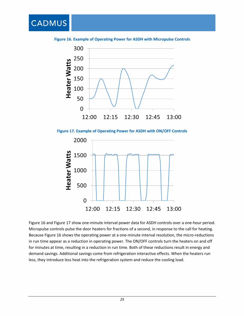
Figure 16. Example of Operating Power for ASDH with Micropulse Controls ............................................ 25
Figure 17. Example of Operating Power for ASDH with ON/OFF Controls ................................................. 25
Figure 18. Key Tasks for Commercial Refrigeration Loadshape Analysis .................................................... 26
Figure 19. ECM Retrofit Measurements (Primary and Secondary) ............................................................. 34
Figure 20. EF Control Measurements (Primary and Secondary Data) ........................................................ 36
Figure 21. ASDH Measurements (Primary and Secondary Data) ................................................................ 37
Figure 22. Metering Period (Primary Data) ................................................................................................. 41
Figure 23. Example of Meter Installation on Evaporator Fans ................................................................... 42
Figure 24. Example of Meter Installation on Door Heaters ........................................................................ 43
Figure 25. Summary of Methods ................................................................................................................ 44
Figure 26. Example Load Duration Curve for EF Motor (Post-installation) ................................................ 46
Figure 27. Average Hourly Baseline Motor Power (Site 10 EF-B) ............................................................... 47
Figure 28. Average Hourly Post-installation Motor Power18 (Site 10 EF-B) ................................................ 47
Figure 29. Average Pre/Post Motor Run Time18 (Site 10 EF-B) ................................................................... 47
Figure 30. Time series of Metered Motor Power (Site 10 EF-B) ................................................................. 47
Figure 31. Average Hourly Baseline Motor Power (Site 3 EF-A) ................................................................. 48
Figure 32. Average Hourly Post-installation Motor Power19 (Site 3 EF-A) .................................................. 48
Figure 33. Average Pre/Post Motor Run Time19 (Site 3 EF-A) ..................................................................... 48
Figure 34. Timeseries of Metered Motor (Site 3 EF-A) ............................................................................... 48
Figure 35. Average Hourly Baseline ASDH Power (Site 6 DH-A) ................................................................. 50
Figure 36. Average Hourly Post-installation ASDH Power20 (Site 6 DH-A) .................................................. 50
Figure 37. Average Pre/post ASDH Run Time20 (Site 6 DH-A) ..................................................................... 50
Figure 38. Timeseries of Metered ASDH Power20 (Site 6 DH-A) ................................................................. 50
Figure 39. Unit Comparison – Average Pre/Post EF Motor Operating Power ............................................ 52
iii
Figure 40. Evaporator Fan Motor Measured Full Load Operating Power vs. Rated Horsepower .............. 53
Figure 41. Unit Comparison – Average Baseline EF Motor Operating Power (W/hp)* .............................. 54
Figure 42. Unit Comparison – Average ECM Operating Power (W/hp)* .................................................... 55
Figure 43. Unit Comparison – Average Baseline EF Motor Run Time (%)*................................................. 56
Figure 44. Unit Comparison – Average ECM Run Time with Controls (%)* ................................................ 57
Figure 45. Unit Comparison – Average Baseline ASDH Operating Power (W/door)* ................................ 58
Figure 46. Unit Comparison – Average Baseline ASDH Run Time (%)* ...................................................... 59
Figure 47. Unit Comparison – Average ASDH Run Time with Controls* .................................................... 60
Figure 48. Analysis Steps for Estimating Refrigeration Interactive Effects ................................................. 62
Figure 49. Equipment Savings Loadshape for ECM Retrofit (1 week) ........................................................ 72
Figure 50. Equipment Savings Loadshape for EF Motor Controls (1 week) ................................................ 74
Figure 51. Equipment Savings Loadshape for ASDH Controls (1 week) ...................................................... 76
Figure 52. Total Savings Loadshape for ECM Retrofit (1 week) .................................................................. 77
Figure 53. Total Savings Loadshape for ECM Retrofit (8760) ..................................................................... 77
Figure 54. TRM Comparison – Interactive Refrigeration Multiplier ........................................................... 78
Figure 55. Quantity of Motors Metered by Rated Horsepower ................................................................. 79
Figure 56. Examples of Poor Evaporator Coil Conditions ........................................................................... 89
Figure 57. Impacts of Airflow Restrictions on Motor Operating Power (Coil=suction, Fan=discharge) ..... 94
iv
Tables Table 1. Final Measurement Sample (Primary and Secondary Data) ........................................................... 3
Table 2. Final Sample by Building Type (Primary Data) ................................................................................ 3
Table 3. Percent of Final Measurement Sample by Case Type ..................................................................... 4
Table 4. Average Parameters – EF Motors .................................................................................................... 6
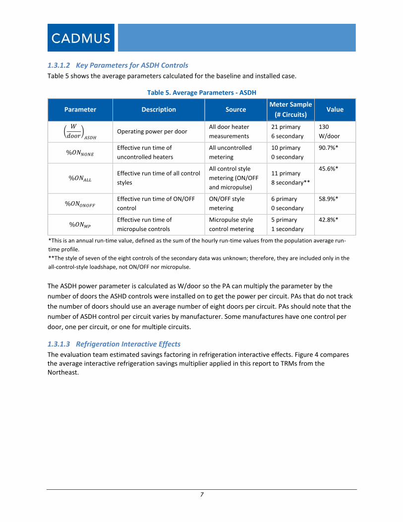
Table 5. Average Parameters - ASDH ............................................................................................................ 7
Table 6. Key Savings Metrics for Evaporator Fan Motor Retrofits ............................................................. 10
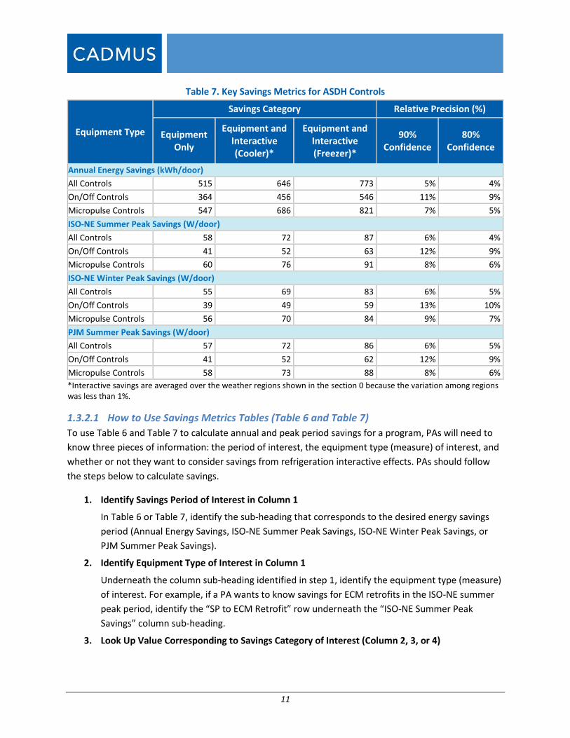
Table 7. Key Savings Metrics for ASDH Controls ......................................................................................... 11
Table 8. Example Measure Savings Results ................................................................................................ 13
Table 9. Program Administrator Data Received ......................................................................................... 27
Table 10. Total Tracked Savings (kWh) by Measure and PA ....................................................................... 28
Table 11. Total Tracked Measures by Measure and PA .............................................................................. 28
Table 12. Average Tracked Unit Savings (kWh) .......................................................................................... 29
Table 13. Number of Unique Measures Installed Per Site .......................................................................... 29
Table 14. Average Number of Measures per Site ....................................................................................... 30
Table 15. CV of Unit Tracked Savings (kWh) ............................................................................................... 30
Table 16. Average Unit-Level Tracked Savings (kW) ................................................................................... 30
Table 17. CV of Average Unit Tracked kW Savings ..................................................................................... 31
Table 18. Metering Data Received .............................................................................................................. 32
Table 19. Final Site Sample by Implementer (Primary Data) ...................................................................... 33
Table 20. Final Sample by Building Type ..................................................................................................... 33
Table 21. ECM Retrofit Measurements by Motor Type and State (Primary and Secondary Data) ............ 35
Table 22. ECM Retrofit Measurements by Building Type (Primary and Secondary Data) .......................... 35
Table 23. EF Control Measurements by Control Type and State (Primary and Secondary Data) ............... 36
Table 24. EF Control Measurements by Building Type (Primary and Secondary Data) .............................. 37
Table 25. ASDH Measurements by Control Type and State (Primary and Secondary Data) ...................... 38
Table 26. ASDH Measurements by Building Type (Primary and Secondary Data)...................................... 38
Table 27. Power Logging Equipment .......................................................................................................... 42
Table 28. Average Parameters – Full Load Operating Power for EF Motors .............................................. 64
Table 29. TRM Comparison – ECM Operating Power (W/motor) ............................................................... 65
Table 30. TRM Comparison – Baseline Motor Operating Power (W/motor) ............................................. 65
Table 31. TRM Comparison – Load Reduction Factor for ECM Retrofits (%) .............................................. 66
Table 32. Average Parameters – Full Load Operating Power for ASDH ...................................................... 66
Table 33. TRM Comparison – ASDH Operating Power (Watts/door) ......................................................... 67
Table 34. Average Parameters – Effective Run Time for EF Motors ........................................................... 67
Table 35. EF Motor Run-time Profiles by Control Type for a Weekday (WD), Saturday (Sat), and Sunday
(Sun) ............................................................................................................................................................ 68
Table 36. TRM Comparison – Load Reduction Factor for EF Motor with Controls (%) .............................. 69
Table 37. Average Parameters – Effective Run Time for ASDH .................................................................. 69
v
Table 38. ASDH Run-time Profiles by Control Type for a Weekday (WD), Saturday (Sat), and Sunday (Sun)
.................................................................................................................................................................... 70
Table 39. TRM Comparison – Load Reduction Factor with ASDH Controls (%) .......................................... 71
Table 40. Calculation Parameters for ECM Retrofit .................................................................................... 72
Table 41. Calculation Parameters for EF Motor Controls ........................................................................... 73
Table 42. Calculation Parameters for ASDH Controls ................................................................................. 75
Table 43. Annual Energy Savings for EF Motors and Controls .................................................................... 80
Table 44. Energy Period Allocations for EF Motors and Controls ............................................................... 81
Table 45. ISO-NE Summer Peak Savings for EF Motors and Controls ......................................................... 82
Table 46. ISO-NE Winter Peak Savings for EF Motors and Controls ........................................................... 82
Table 47. PJM Peak Savings for EF Motors and Controls ............................................................................ 83
Table 48. Annual Energy Savings for ASDH Controls .................................................................................. 83
Table 49. Energy Period Savings Allocations for ASDH Controls ................................................................ 84
Table 50. ISO-NE Summer Peak Savings for ASDH Controls ....................................................................... 84
Table 51. ISO-NE Winter Peak Savings for ASDH Controls .......................................................................... 85
Table 52. PJM Summer Peak Savings for ASDH Controls ............................................................................ 85
Table 53. Descriptions of Secondary Data Sources ..................................................................................... 90
vi
Acronym Glossary
Acronym Definition ASDH Anti-sweat door heater
CRL Commercial refrigeration loadshape (i.e., this study)
DMI
Demand Management Institute – provides expertise on energy-related technical
assistance, ranging from cost-benefit analysis of a single energy efficiency opportunity, to
comprehensive strategies for reduced energy consumption in a campus of facilities
ECM Electronically-commutated motor
EF Evaporator fan
EM&V Evaluation, measurement, and verification
GEE Global Energy Efficiency – a large volume, full-service energy management company in
New York
ISO-NE
Independent System Operator, New England, Inc. – is an independent, non-profit regional
transmission organization (RTO), serving Connecticut, Maine, Massachusetts, New
Hampshire, Rhode Island and Vermont
NEEP
Northeast Energy Efficiency Partnerships – a non-profit whose mission is to serve the
Northeast and Mid-Atlantic to accelerate energy efficiency in the building sector through
public policy, program strategies and education.
NRM National Resource Management, Inc. – a large volume refrigeration retrofit contractor in
the northeast.
PA Program administrator
PJM
Pennsylvania-New Jersey-Maryland Interconnection – a regional transmission organization
(RTO) that coordinates the movement of wholesale electricity in all or parts of Delaware,
Illinois, Indiana, Kentucky, Maryland, Michigan, New Jersey, North Carolina, Ohio,
Pennsylvania, Tennessee, Virginia, West Virginia and the District of Columbia
PSC Permanent split capacitor
SP Shaded pole
TRM Technical Reference Manual
1
1 Executive Summary
The Northeast Energy Efficiency Partnerships (NEEP) Regional Evaluation, Measurement, and
Verification Forum (EM&V Forum) conducts research studies to support energy efficiency programs and
policy in the Northeast and Mid-Atlantic states. In 2014, the EM&V Forum and its sponsors
commissioned this commercial refrigeration loadshape (CRL) study to determine the hourly energy and
demand impacts of three common commercial refrigeration retrofit measures commonly installed
through energy efficiency programs in the Northeast and Mid-Atlantic states:
Electronically commutated motors (ECMs) installed on evaporator fans in coolers and freezers
Evaporator fan (EF) controls
Anti-sweat door heater (ASDH) controls
The EM&V Forum and its sponsors chose to study these three measures because they reliably produce
commercial energy and demand savings, yet little or no evaluations using empirical evidence exist. This
study employed pre- and post-installation metering to evaluate the savings. Due to the regional nature
of the study, the findings provide insights on a variety of manufacturers, products, and types of
technologies.
Cadmus and the Demand Management Institute (DMI), the evaluation team, worked with the EM&V
Forum’s Technical Committee to complete this study. This report describes the study objectives,
methods, and results and the evaluation team’s recommendations for future implementation and
evaluation of energy-efficient measures on commercial refrigeration equipment.
1.1 Objectives The EM&V Forum commissioned this study to assess the annual, peak, and hourly demand impacts from
the three commercial refrigeration retrofit measures most commonly installed through energy efficiency
programs in the Northeast and Mid-Atlantic states.1 Through primary and secondary data collection and
analysis, the evaluation team developed hourly demand savings estimates—savings loadshapes—for
ECM retrofits, evaporator fan controls, and ASDH controls installed on commercial refrigeration
equipment. The evaluation team used these loadshapes to calculate key savings metrics, including
annual energy savings and demand savings during peak periods. The evaluation team also created a
loadshape calculation tool, which enables users to select whether to include interactive refrigeration
savings, determine if the refrigerated case is a cooler or freezer, and compute the savings for any
specific period of interest throughout the year.
The EM&V Forum provides these study results and primary data to its members to support activities
including regulatory filings for energy efficiency programs, developing or updating technical reference
1 The study was sponsored by eleven states—Connecticut, Delaware, Maine, Maryland, Massachusetts, New
Hampshire, New Jersey, New York, Pennsylvania, Rhode Island, and Vermont—and Washington, D.C.
2
manuals (TRMs), supporting demand resource values submitted to forward-capacity markets, and air
emission impacts.
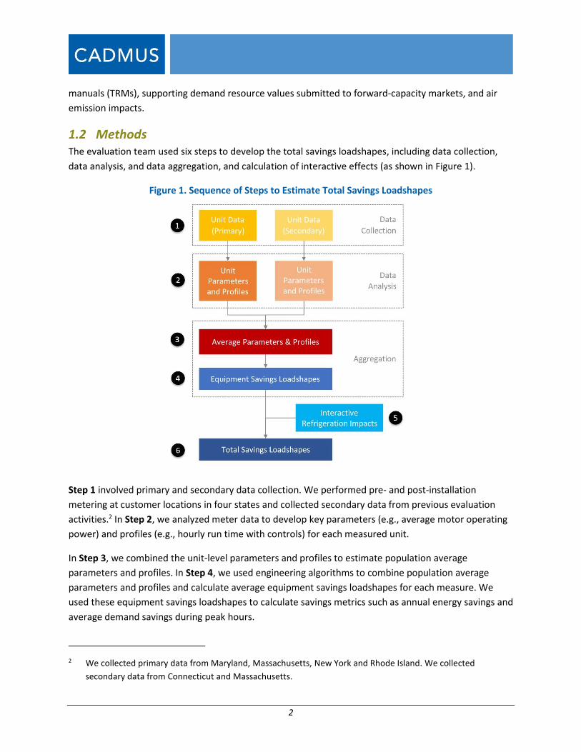
1.2 Methods The evaluation team used six steps to develop the total savings loadshapes, including data collection,
data analysis, and data aggregation, and calculation of interactive effects (as shown in Figure 1).
Figure 1. Sequence of Steps to Estimate Total Savings Loadshapes
Step 1 involved primary and secondary data collection. We performed pre- and post-installation
metering at customer locations in four states and collected secondary data from previous evaluation
activities.2 In Step 2, we analyzed meter data to develop key parameters (e.g., average motor operating
power) and profiles (e.g., hourly run time with controls) for each measured unit.
In Step 3, we combined the unit-level parameters and profiles to estimate population average
parameters and profiles. In Step 4, we used engineering algorithms to combine population average
parameters and profiles and calculate average equipment savings loadshapes for each measure. We
used these equipment savings loadshapes to calculate savings metrics such as annual energy savings and
average demand savings during peak hours.
2 We collected primary data from Maryland, Massachusetts, New York and Rhode Island. We collected
secondary data from Connecticut and Massachusetts.
3
In Step 5, we estimated the interactive effects of the retrofit measures on refrigeration system loads
and power. Finally, in Step 6, we combined the refrigeration interactive effects with the equipment
savings loadshapes to estimate the total savings loadshapes.
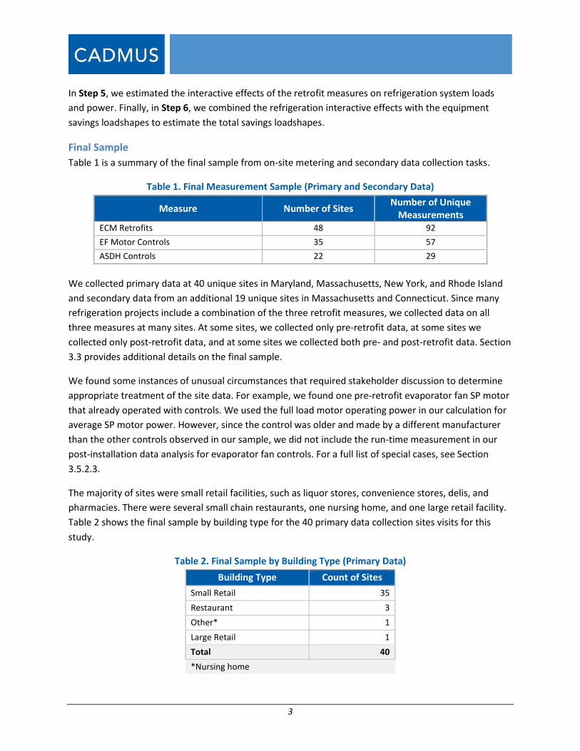
Final Sample
Table 1 is a summary of the final sample from on-site metering and secondary data collection tasks.
Table 1. Final Measurement Sample (Primary and Secondary Data)
Measure Number of Sites Number of Unique
Measurements ECM Retrofits 48 92
EF Motor Controls 35 57
ASDH Controls 22 29
We collected primary data at 40 unique sites in Maryland, Massachusetts, New York, and Rhode Island
and secondary data from an additional 19 unique sites in Massachusetts and Connecticut. Since many
refrigeration projects include a combination of the three retrofit measures, we collected data on all
three measures at many sites. At some sites, we collected only pre-retrofit data, at some sites we
collected only post-retrofit data, and at some sites we collected both pre- and post-retrofit data. Section
3.3 provides additional details on the final sample.
We found some instances of unusual circumstances that required stakeholder discussion to determine
appropriate treatment of the site data. For example, we found one pre-retrofit evaporator fan SP motor
that already operated with controls. We used the full load motor operating power in our calculation for
average SP motor power. However, since the control was older and made by a different manufacturer
than the other controls observed in our sample, we did not include the run-time measurement in our
post-installation data analysis for evaporator fan controls. For a full list of special cases, see Section
3.5.2.3.
The majority of sites were small retail facilities, such as liquor stores, convenience stores, delis, and
pharmacies. There were several small chain restaurants, one nursing home, and one large retail facility.
Table 2 shows the final sample by building type for the 40 primary data collection sites visits for this
study.
Table 2. Final Sample by Building Type (Primary Data)
Building Type Count of Sites
Small Retail 35
Restaurant 3
Other* 1
Large Retail 1
Total 40
*Nursing home
4
Site visits took place in BGE territory in Maryland where measures were installed by National Resource
Management, Inc. (NRM), Anthony International, and Johnson Controls; National Grid territory in
Massachusetts and Rhode Island with measures installed by NRM; and Con Edison territory in New York
with measures installed by Global Energy Efficiency (GEE) and Willdan. Measurements for the 19
secondary sites took place in National Grid territory in MA and Eversource territory in Connecticut.34
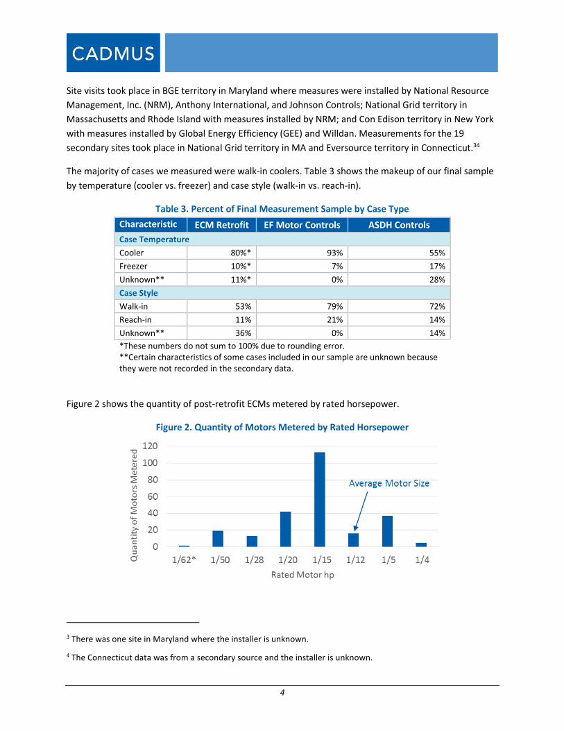
The majority of cases we measured were walk-in coolers. Table 3 shows the makeup of our final sample
by temperature (cooler vs. freezer) and case style (walk-in vs. reach-in).
Table 3. Percent of Final Measurement Sample by Case Type
Characteristic ECM Retrofit EF Motor Controls ASDH Controls
Case Temperature
Cooler 80%* 93% 55%
Freezer 10%* 7% 17%
Unknown** 11%* 0% 28%
Case Style
Walk-in 53% 79% 72%
Reach-in 11% 21% 14%
Unknown** 36% 0% 14%
*These numbers do not sum to 100% due to rounding error. **Certain characteristics of some cases included in our sample are unknown because they were not recorded in the secondary data.
Figure 2 shows the quantity of post-retrofit ECMs metered by rated horsepower.
Figure 2. Quantity of Motors Metered by Rated Horsepower
3 There was one site in Maryland where the installer is unknown.
4 The Connecticut data was from a secondary source and the installer is unknown.

5
*Motors rated below 1/50 hp are typically reported in watts; value presented is equivalent horsepower.
The majority of installed motors are rated at 1/15 horsepower, but we observed motors ranging from 12
Watts (equivalent to 1/62 hp) to 1/4 hp. The average rated horsepower from our sample was 1/12 hp. If
the program administrator cannot track the installed motor horsepower, we recommend using 1/15 hp
as the standard value to evaluate savings.
Unit Parameters and Profiles
To estimate savings for evaporator fan motors and ASDHs, the evaluation team used primary and
secondary data to assess key parameters (single values) and profiles (hourly values based on time of day
and day of week). The average full load operating power is a key parameter to determine the power
draw of motors and door heaters. The effective hourly run-time profiles provide hourly estimates of the
operating status of equipment with or without controls. The evaluation team examined the unit
parameters and profiles shown in Figure 3.
Figure 3. Unit Parameters and Profiles
* Shaded pole (SP) motors represent the baseline case for evaporator fans.
1.3 Results The evaluation team created a loadshape calculation tool to estimate hourly energy and demand savings
for each retrofit measure. The tool enables the user to select whether to include interactive
refrigeration savings, estimate savings separately for coolers or freezers, and compute the savings for
any specific period of interest throughout the year.
This report presents annual energy and peak demand savings for three peak periods—ISO-NE summer,
ISO-NE winter, and PJM summer—for each measure type, and refrigerator space type (cooler or
freezer).5
5 ISO-NE summer comprises 1:00 PM to 5:00 PM on non-holiday weekdays in June through August, ISO-NE
winter comprises 5:00 PM to 7:00 PM on non-holiday weekdays in December and January, and PJM summer
comprises 2:00 PM to 6:00 PM on non-holiday weekdays in June through September.
EF Motor ECM Retrofits and Controls
•Pre/Post EF Motor Operating Power
•Operating Power for SP Motors (per HP)
•Operating Power for ECMs (per HP)
•EF Motor Run Time without Controls
•ECM Run Time with Controls
ASDH Controls
•ADSH Operating Power
•ASDH Run Time without Controls
•ASDH Run Time with Controls
•ON/OFF controls
•Micropulse controls
•Unknown controls
6
1.3.1 Key Findings
This study developed key parameters for estimating savings from ECM Retrofits, EF Controls, and ASDH
controls including the refrigeration interactive effects. PAs may use these values to update parameters
in their TRMs and to estimate savings values for the three retrofit measures.
1.3.1.1 Key Parameters for ECM Retrofits and EF Controls
Table 4 shows the average parameters calculated for the baseline and installed case.
Table 4. Average Parameters – EF Motors
Parameter Description Source Meter Sample
(# Circuits) Value
(𝑊𝑆𝑃 − 𝑊𝐸𝐶𝑀
𝑊𝐸𝐶𝑀
) × 100 Percentage change in power
relative to post wattage
Pre/post metering
only*
9 primary
0 secondary 157%
(𝑊
ℎ𝑝)
𝐸𝐶𝑀
ECM power normalized by
horsepower (see Figure 42)
All ECM
measurements
42 primary
24 secondary 758 W/hp
(𝑊
ℎ𝑝)
𝑆𝑃
SP motor power normalized
by horsepower (see Figure
45)
All SP motor
measurements
13 primary
5 secondary 2,088 W/hp
%𝑂𝑁𝑁𝑂𝑁𝐸 Effective run time of
uncontrolled motors
All uncontrolled
metering (ECM and
SP)
32 primary
0 secondary
97.8%**
%𝑂𝑁𝐴𝐿𝐿 Effective run time of all
control styles
All control style
metering (ON/OFF
and multi-speed)
25 primary
0 secondary
66.5%**
%𝑂𝑁𝑂𝑁𝑂𝐹𝐹 Effective run time of
ON/OFF style control
ON/OFF style
control metering
12 primary
0 secondary
63.6%**
%𝑂𝑁𝑀𝑆 Effective run time of multi-
speed style controls
Multi-speed style
control metering
13 primary
0 secondary
69.2%**
* We calculated this parameter by first computing 𝑊𝑆𝑃−𝑊𝐸𝐶𝑀
𝑊𝐸𝐶𝑀 for each unit for which we collected both pre and post
measurements and then averaging these nine values.
** This is an annual run-time value defined as the sum of the hourly run-time values from the population average run-
time profile.
The EF motor power parameters are calculated as W/hp so the program administrator (PA) can multiply
the parameter by the installed motor horsepower to calculate the W/motor for the baseline case and
installed case. PAs that do not track rated horsepower information should use a default motor size of
1/15 hp based on the most common motor size observed in this study (see Figure 2). The baseline case
for evaporator fan motors is assumed to be shaded pole (SP) motors because more than 90% of
observed baseline motors were SP.
7
1.3.1.2 Key Parameters for ASDH Controls
Table 5 shows the average parameters calculated for the baseline and installed case.
Table 5. Average Parameters - ASDH
Parameter Description Source Meter Sample
(# Circuits) Value
(𝑊
𝑑𝑜𝑜𝑟)
𝐴𝑆𝐷𝐻 Operating power per door
All door heater
measurements
21 primary
6 secondary
130
W/door
%𝑂𝑁𝑁𝑂𝑁𝐸 Effective run time of
uncontrolled heaters
All uncontrolled
metering
10 primary
0 secondary
90.7%*
%𝑂𝑁𝐴𝐿𝐿 Effective run time of all control
styles
All control style
metering (ON/OFF
and micropulse)
11 primary
8 secondary**
45.6%*
%𝑂𝑁𝑂𝑁𝑂𝐹𝐹 Effective run time of ON/OFF
control
ON/OFF style
metering
6 primary
0 secondary
58.9%*
%𝑂𝑁𝑀𝑃 Effective run time of
micropulse controls
Micropulse style
control metering
5 primary
1 secondary
42.8%*
*This is an annual run-time value, defined as the sum of the hourly run-time values from the population average run-
time profile.
**The style of seven of the eight controls of the secondary data was unknown; therefore, they are included only in the
all-control-style loadshape, not ON/OFF nor micropulse.
The ASDH power parameter is calculated as W/door so the PA can multiply the parameter by the
number of doors the ASHD controls were installed on to get the power per circuit. PAs that do not track
the number of doors should use an average number of eight doors per circuit. PAs should note that the
number of ASDH control per circuit varies by manufacturer. Some manufactures have one control per
door, one per circuit, or one for multiple circuits.
1.3.1.3 Refrigeration Interactive Effects
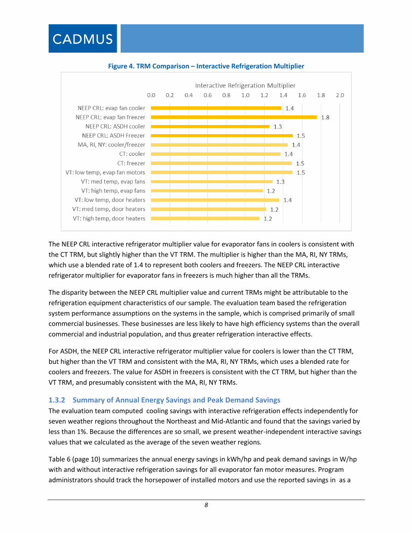
The evaluation team estimated savings factoring in refrigeration interactive effects. Figure 4 compares the average interactive refrigeration savings multiplier applied in this report to TRMs from the Northeast.
8
Figure 4. TRM Comparison – Interactive Refrigeration Multiplier
The NEEP CRL interactive refrigerator multiplier value for evaporator fans in coolers is consistent with
the CT TRM, but slightly higher than the VT TRM. The multiplier is higher than the MA, RI, NY TRMs,
which use a blended rate of 1.4 to represent both coolers and freezers. The NEEP CRL interactive
refrigerator multiplier for evaporator fans in freezers is much higher than all the TRMs.
The disparity between the NEEP CRL multiplier value and current TRMs might be attributable to the
refrigeration equipment characteristics of our sample. The evaluation team based the refrigeration
system performance assumptions on the systems in the sample, which is comprised primarily of small
commercial businesses. These businesses are less likely to have high efficiency systems than the overall
commercial and industrial population, and thus greater refrigeration interactive effects.
For ASDH, the NEEP CRL interactive refrigerator multiplier value for coolers is lower than the CT TRM,
but higher than the VT TRM and consistent with the MA, RI, NY TRMs, which uses a blended rate for
coolers and freezers. The value for ASDH in freezers is consistent with the CT TRM, but higher than the
VT TRM, and presumably consistent with the MA, RI, NY TRMs.
1.3.2 Summary of Annual Energy Savings and Peak Demand Savings
The evaluation team computed cooling savings with interactive refrigeration effects independently for
seven weather regions throughout the Northeast and Mid-Atlantic and found that the savings varied by
less than 1%. Because the differences are so small, we present weather-independent interactive savings
values that we calculated as the average of the seven weather regions.
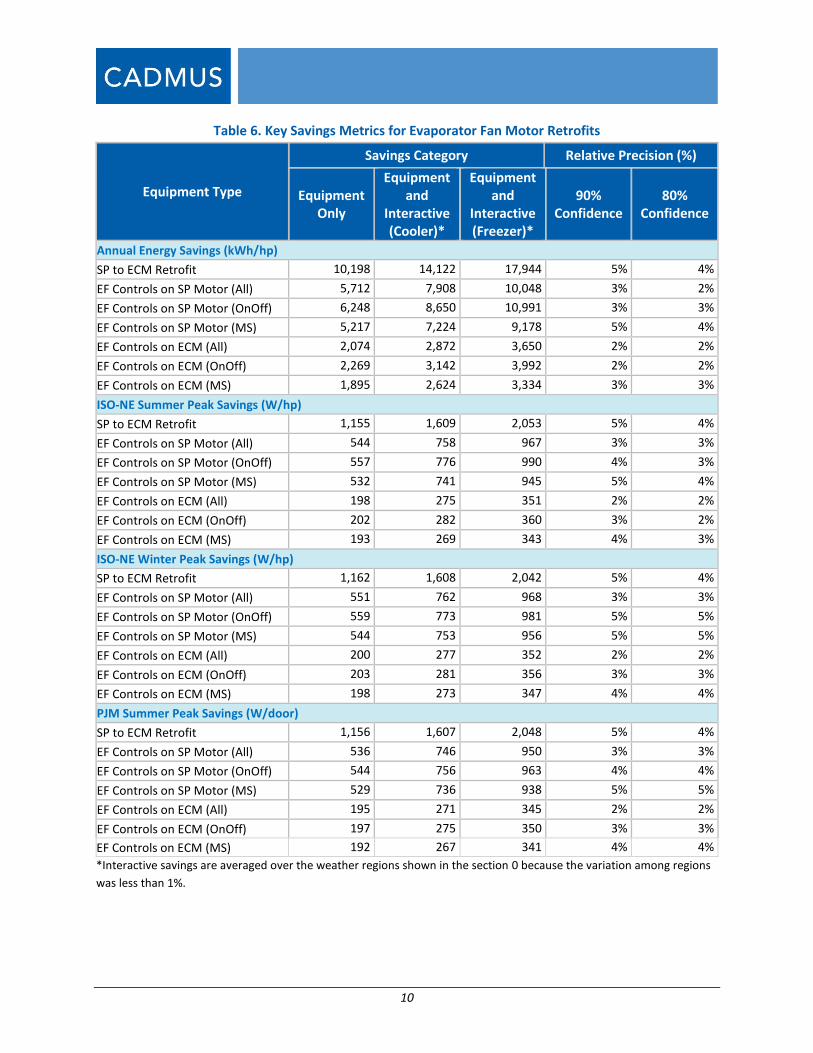
Table 6 (page 10) summarizes the annual energy savings in kWh/hp and peak demand savings in W/hp
with and without interactive refrigeration savings for all evaporator fan motor measures. Program
administrators should track the horsepower of installed motors and use the reported savings in as a
9
multiplier. Annual and peak demand savings from the SP to ECM retrofit and ECM controls are additive if
the measures are done together.
Table 7 shows the annual energy savings in kWh/door and peak demand savings in W/door with and
without interactive cooling savings for both types of ASDH controls as well as a single overall average.
Program administrators should track the number of doors per ASDH control installed and use the
reported savings in Table 7 as a multiplier. PAs should note that the number of doors per ASDH control
varies by manufacturer and application. Some manufactures have one control per door, one control per
circuit, or one control for multiple circuits.
10
Table 6. Key Savings Metrics for Evaporator Fan Motor Retrofits
Equipment Type
Savings Category Relative Precision (%)
Equipment Only
Equipment and
Interactive (Cooler)*
Equipment and
Interactive (Freezer)*
90% Confidence
80% Confidence
Annual Energy Savings (kWh/hp)
SP to ECM Retrofit 10,198 14,122 17,944 5% 4%
EF Controls on SP Motor (All) 5,712 7,908 10,048 3% 2%
EF Controls on SP Motor (OnOff) 6,248 8,650 10,991 3% 3%
EF Controls on SP Motor (MS) 5,217 7,224 9,178 5% 4%
EF Controls on ECM (All) 2,074 2,872 3,650 2% 2%
EF Controls on ECM (OnOff) 2,269 3,142 3,992 2% 2%
EF Controls on ECM (MS) 1,895 2,624 3,334 3% 3%
ISO-NE Summer Peak Savings (W/hp)
SP to ECM Retrofit 1,155 1,609 2,053 5% 4%
EF Controls on SP Motor (All) 544 758 967 3% 3%
EF Controls on SP Motor (OnOff) 557 776 990 4% 3%
EF Controls on SP Motor (MS) 532 741 945 5% 4%
EF Controls on ECM (All) 198 275 351 2% 2%
EF Controls on ECM (OnOff) 202 282 360 3% 2%
EF Controls on ECM (MS) 193 269 343 4% 3%
ISO-NE Winter Peak Savings (W/hp)
SP to ECM Retrofit 1,162 1,608 2,042 5% 4%
EF Controls on SP Motor (All) 551 762 968 3% 3%
EF Controls on SP Motor (OnOff) 559 773 981 5% 5%
EF Controls on SP Motor (MS) 544 753 956 5% 5%
EF Controls on ECM (All) 200 277 352 2% 2%
EF Controls on ECM (OnOff) 203 281 356 3% 3%
EF Controls on ECM (MS) 198 273 347 4% 4%
PJM Summer Peak Savings (W/door)
SP to ECM Retrofit 1,156 1,607 2,048 5% 4%
EF Controls on SP Motor (All) 536 746 950 3% 3%
EF Controls on SP Motor (OnOff) 544 756 963 4% 4%
EF Controls on SP Motor (MS) 529 736 938 5% 5%
EF Controls on ECM (All) 195 271 345 2% 2%
EF Controls on ECM (OnOff) 197 275 350 3% 3%
EF Controls on ECM (MS) 192 267 341 4% 4%
*Interactive savings are averaged over the weather regions shown in the section 0 because the variation among regions
was less than 1%.
11
Table 7. Key Savings Metrics for ASDH Controls
Equipment Type
Savings Category Relative Precision (%)
Equipment Only
Equipment and Interactive (Cooler)*
Equipment and Interactive (Freezer)*
90% Confidence
80% Confidence
Annual Energy Savings (kWh/door)
All Controls 515 646 773 5% 4%
On/Off Controls 364 456 546 11% 9%
Micropulse Controls 547 686 821 7% 5%
ISO-NE Summer Peak Savings (W/door)
All Controls 58 72 87 6% 4%
On/Off Controls 41 52 63 12% 9%
Micropulse Controls 60 76 91 8% 6%
ISO-NE Winter Peak Savings (W/door)
All Controls 55 69 83 6% 5%
On/Off Controls 39 49 59 13% 10%
Micropulse Controls 56 70 84 9% 7%
PJM Summer Peak Savings (W/door)
All Controls 57 72 86 6% 5%
On/Off Controls 41 52 62 12% 9%
Micropulse Controls 58 73 88 8% 6%
*Interactive savings are averaged over the weather regions shown in the section 0 because the variation among regions was less than 1%.
1.3.2.1 How to Use Savings Metrics Tables (Table 6 and Table 7)
To use Table 6 and Table 7 to calculate annual and peak period savings for a program, PAs will need to
know three pieces of information: the period of interest, the equipment type (measure) of interest, and
whether or not they want to consider savings from refrigeration interactive effects. PAs should follow
the steps below to calculate savings.
1. Identify Savings Period of Interest in Column 1
In Table 6 or Table 7, identify the sub-heading that corresponds to the desired energy savings
period (Annual Energy Savings, ISO-NE Summer Peak Savings, ISO-NE Winter Peak Savings, or
PJM Summer Peak Savings).
2. Identify Equipment Type of Interest in Column 1
Underneath the column sub-heading identified in step 1, identify the equipment type (measure)
of interest. For example, if a PA wants to know savings for ECM retrofits in the ISO-NE summer
peak period, identify the “SP to ECM Retrofit” row underneath the “ISO-NE Summer Peak
Savings” column sub-heading.
3. Look Up Value Corresponding to Savings Category of Interest (Column 2, 3, or 4)
12
Depending on whether the PA is interested in calculating savings with or without refrigeration
interactive effects, look up the row corresponding to the savings category of interest (column 2,
3, or 4). For instance, if the PA wants to know the ISO-NE summer peak savings for ECM retrofits
in cooler cases including refrigeration interactive effects, look up the value in the third column
(“Equipment and Interactive (Cooler)”). In this example, the value is 1,609 W/hp.
4. Multiply Value by Horsepower Per Motor or Quantity of Doors Per Control
a. Evaporator Fans (Table 6): If the ECM motor horsepower for the program is known,
multiply the value found in step 3 by the rated horsepower. If the ECM motor
horsepower is unknown, multiply the value found in step 3 by 1/15 hp (the most often
installed ECM motor size observed in this evaluation). Table 8 shows example results as
savings per measure for equipment in a cooler case and using the ISO-NE summer peak
period.
b. ASDH Controls (Table 7). If the quantity of doors per ASDH control is known, multiply
the value found in step 3 by the quantity of doors per ASDH control. If the quantity of
doors per ASDH control is unknown, multiply the value found in step 3 by eight doors
(the average number of doors per ASDH control observed in this evaluation). Table 8
shows example results as savings per measure for equipment in a cooler case and using
the ISO-NE summer peak period.
5. Multiply Result by Quantity of Measures in Program
Multiply the results calculated in step 4 by the quantity of units installed in the program to
calculate program savings for that measure.
Table 8 shows example results as savings per measure for equipment in a cooler case and using the ISO-NE summer peak period.
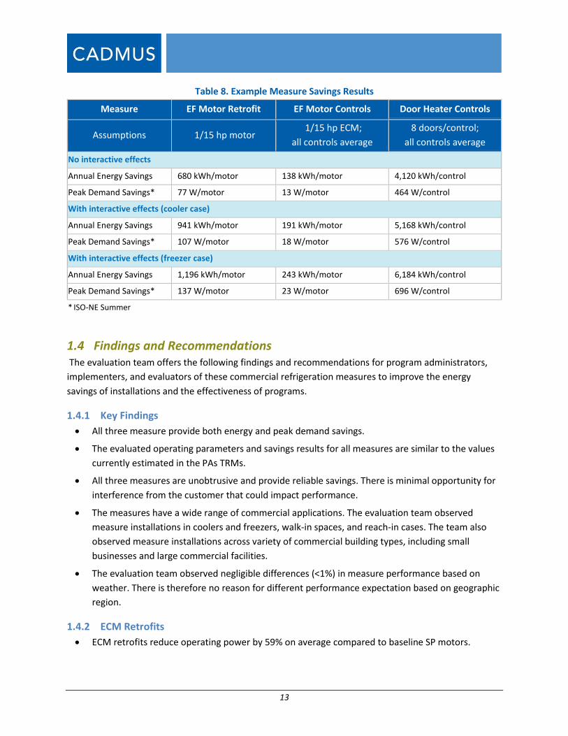
13
Table 8. Example Measure Savings Results
Measure EF Motor Retrofit EF Motor Controls Door Heater Controls
Assumptions 1/15 hp motor 1/15 hp ECM;
all controls average
8 doors/control;
all controls average
No interactive effects
Annual Energy Savings 680 kWh/motor 138 kWh/motor 4,120 kWh/control
Peak Demand Savings* 77 W/motor 13 W/motor 464 W/control
With interactive effects (cooler case)
Annual Energy Savings 941 kWh/motor 191 kWh/motor 5,168 kWh/control
Peak Demand Savings* 107 W/motor 18 W/motor 576 W/control
With interactive effects (freezer case)
Annual Energy Savings 1,196 kWh/motor 243 kWh/motor 6,184 kWh/control
Peak Demand Savings* 137 W/motor 23 W/motor 696 W/control
* ISO-NE Summer
1.4 Findings and Recommendations The evaluation team offers the following findings and recommendations for program administrators,
implementers, and evaluators of these commercial refrigeration measures to improve the energy
savings of installations and the effectiveness of programs.
1.4.1 Key Findings
All three measure provide both energy and peak demand savings.
The evaluated operating parameters and savings results for all measures are similar to the values
currently estimated in the PAs TRMs.
All three measures are unobtrusive and provide reliable savings. There is minimal opportunity for
interference from the customer that could impact performance.
The measures have a wide range of commercial applications. The evaluation team observed
measure installations in coolers and freezers, walk-in spaces, and reach-in cases. The team also
observed measure installations across variety of commercial building types, including small
businesses and large commercial facilities.
The evaluation team observed negligible differences (<1%) in measure performance based on
weather. There is therefore no reason for different performance expectation based on geographic
region.
1.4.2 ECM Retrofits
ECM retrofits reduce operating power by 59% on average compared to baseline SP motors.
14
Uncontrolled evaporator fan motors operate continuously and therefore adding controls is a good
measure for both annual energy and peak demand savings.
Only two of the observed baseline motors were PSC. Implementation contractors confirmed they
are less likely to replace baseline PSC motors because the replacement is less cost-effective
compared to SP replacements. Program administrators that use a blended SP/permanent split
capacitor (PSC) baseline should consider using a SP only baseline.6
The majority of installed motors are rated at 1/15 horsepower, but we observed motors ranging
from 12 Watts (equivalent to 1/62 hp) to 1/4 hp. The average rated horsepower from our sample
was 1/12 hp.
Operating power varies for both baseline SP motors and uncontrolled ECMs. This variation is
caused by multiple factors, including differences in rated motor horsepower and efficiency,
diameter and pitch of attached fans, and airflow restrictions. Cadmus tested the impact of airflow
restrictions on motor power. Refer for Appendix B. Airflow Restriction Testing for the results of
the testing. See Section 3.5.2.1 for more detail on the observed variation in operating power.
The rated horsepower of pre-installation and post-installation motors do not always match. For
example, a 1/15-hp SP motor might be replaced with a 1/20-hp ECM, or vice versa. This is due to
geometrical constraints and equipment availability.
One pre-retrofit small grocery site (Site 27. EF-A: Small Grocery) had uncontrolled SP motors that
exhibited an average run time of 51%. We confirmed that the motors did not have controls but
noted that the power consumption fluctuated rapidly and turned off frequently. This indicated the
motor was malfunctioning, which is expected for a small percentage of baseline condition motors.
1.4.3 Evaporator Fan Controls
Evaporator fan controls reduce run time by 32% compared to fans without controls.
Controlled evaporator fan motors operate more frequently during peak periods than periods of
inactivity, but continue to turn on and off throughout the day and are therefore still a good
measure for peak demand savings.
The average run time for controlled motors varies. This variation is caused by multiple factors,
including the control type (ON/OFF style controls which vary the runtime of the motor, versus
multi-speed controls which vary the speed and runtime of the motor), space temperature settings,
and condition of refrigeration equipment. See Section 3.5.2.1 for more detail on the observed
variation in operating power.
The two types of EF controls (ON/OFF and multi-speed) perform differently. ON/OFF controls
resulted in slightly greater energy and peak demand savings than multi-speed controls.
6 Contractors confirmed SP motors are the predominant equipment used on evaporator fan motors for commercial
refrigeration applications. Since they are less efficient than PSC motors, they are also more likely to be
targeted for upgrades.

15
At two of the sites we included in our analysis, controls were disconnected by the customer.
Future metering studies of controls such as these should include investigations of customer
behavior to understand whether controls are routinely disconnected by the customer, and if so,
the reasons why.
1.4.4 Anti-Sweat Door Heater Controls
ASDH controls reduce run time by 45% compared to door heaters without controls.
Controlled ASDHs operate more frequently during peak periods than periods of inactivity, but
continue to turn on and off throughout the day and are therefore still a good measure for peak
demand savings.
The two types of door heater controls (micropulse and ON/OFF) perform differently. Micropulse
controls resulted in greater energy and peak demand savings than ON/OFF controls.
There is variation in the run time of uncontrolled ASDH due to manual operation. At one site (2.
DH-A: Liquor Store), site personnel manually turned the heaters off every night. Through
discussions with contractors, we confirmed this is fairly common operating condition (Section
3.5.2.2).
The average run time of controlled ASDH varies. This is caused by a variety of factors including
type of control and type of sensor.
ASDH operating power varies depending on the make, model, and condition of the heater.
Three sites with the same control manufacturer and implementation contractor exhibited no
savings despite installed controls.
1.4.5 Recommendations
We recommend the PAs adopt the savings estimates from this study as TRM estimates for the
average population or use some of the individual savings parameters developed. Based on our
review of PA tracking data, our estimates are representative of the case types (coolers vs. freezers
and walk-ins vs. reach-ins) in which measures are installed. We recommend PAs continue to track
these differentiators and recommend additional evaluation research to grow the sample and
develop case-specific results.
Current PA estimates of savings are inconsistent in the region due to a variety of sources of
assumptions. However, and the evaluation team recommends all PAs adopt the savings results
from this study, which represent the current, measured equipment performance in the region.
Estimates between PAs should only vary by controller style, if applicable. Controls produced by
different manufacturers operate using different strategies, which we observed to impact
performance. We recommend sampling different control types during any future evaluations and
that implementers record manufacturer and model information on all metered units.
Cadmus’ literature review found few to no studies with pre- and post-installation data, making this
the first study with empirical evidence for these three measures. We recommend that any future
16
studies be designed to supplement the data from this study, to increase sample sizes, given the
range of performance observed in this study.
To facilitate future evaluations and updates to savings evaluations, we recommend that
implementers record baseline motor type, horsepower, manufacturer, model, and customer
behavior as part of an ongoing data collection protocol.
The power consumed by evaporator fan motors varied significantly between cases due to a variety
of factors likely including rated hp, fan size, and airflow restrictions. Measurements of pre- and
post-installation operation on single units gave the most reliable data on the impact of ECM
retrofits. We recommend that in future studies, PAs work with implementation contractors to
facilitate targeting measurements of pre- and post-installation data for each unit.
Because the evaporator fan motors and ASDHs are located entirely within air-conditioned spaces,
we do not expect the measure performance to vary significantly throughout the year. However,
we only collected data during the summer and fall; to confirm this hypothesis we would require
additional metering data from the winter and spring on the same units.
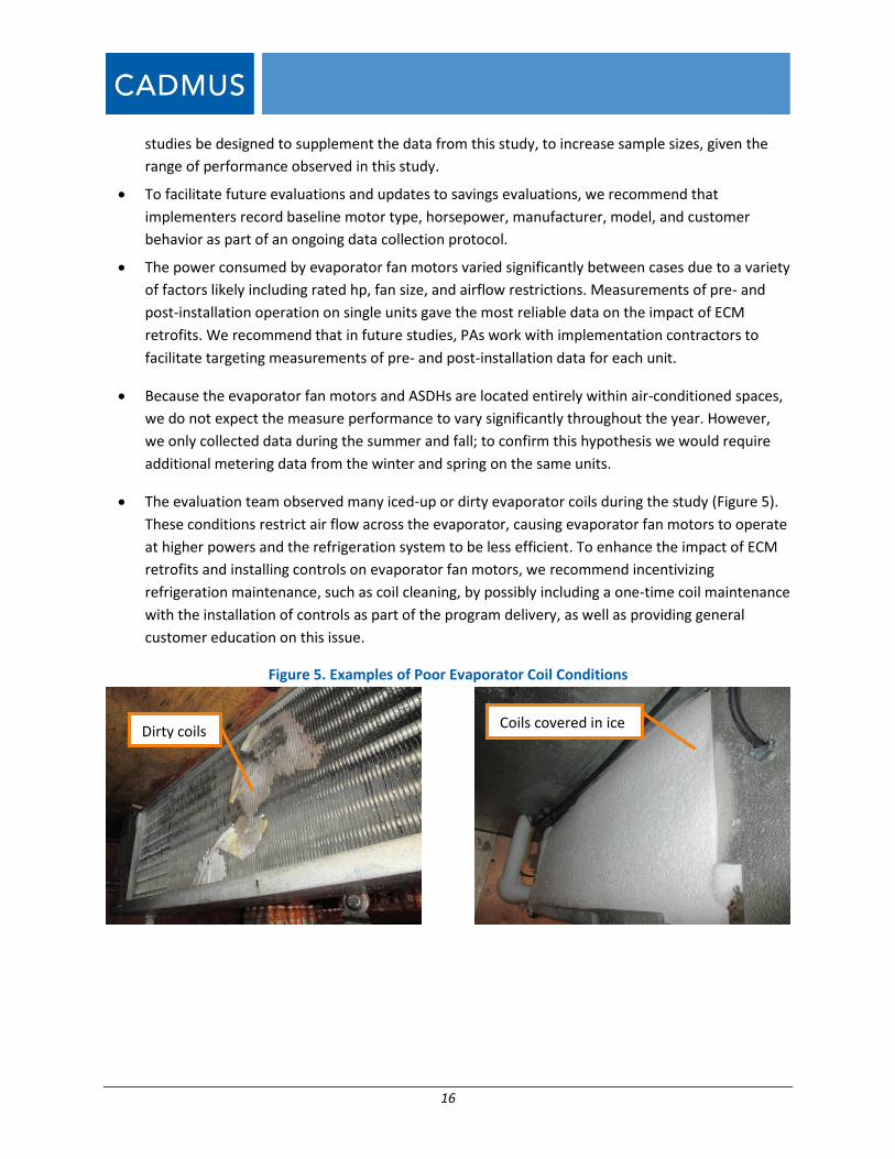
The evaluation team observed many iced-up or dirty evaporator coils during the study (Figure 5).
These conditions restrict air flow across the evaporator, causing evaporator fan motors to operate
at higher powers and the refrigeration system to be less efficient. To enhance the impact of ECM
retrofits and installing controls on evaporator fan motors, we recommend incentivizing
refrigeration maintenance, such as coil cleaning, by possibly including a one-time coil maintenance
with the installation of controls as part of the program delivery, as well as providing general
customer education on this issue.
Figure 5. Examples of Poor Evaporator Coil Conditions
Dirty coils Coils covered in ice
17
2 Introduction
The commercial refrigeration loadshape (CRL) study is the fourth in a series of savings loadshape studies
sponsored by NEEP. These studies evaluate the loadshapes of efficient technologies implemented
through energy efficiency programs in the Northeast and Mid-Atlantic states. This CRL study examines
the annual, peak, and hourly electricity savings achieved by three commercial refrigeration measures
commonly installed in commercial buildings throughout the Northeast and Mid-Atlantic states, including
Connecticut, Delaware, Maine, Maryland, Massachusetts, New Hampshire, New Jersey, New York,
Pennsylvania, Rhode Island, and Vermont, and Washington D.C. The three measures are electrically
commutated motor (ECM) evaporator fan retrofits, evaporator fan (EF) motor controls, and anti-sweat
door heater (ASDH) controls.
2.1 NEEP EM&V Forum The Northeast Energy Efficiency Partnerships (NEEP) is a nonprofit organization established to promote
energy efficiency throughout the Northeast and Mid-Atlantic states.7 NEEP created the Regional
Evaluation, Measurement, and Verification Forum (EM&V Forum) in 2008 “to support the development
and use of consistent protocols to evaluate, measure, verify, and report the savings, costs, and emission
impacts of energy efficiency and other demand-side resources.”
In particular, the EM&V Forum facilitates joint research and evaluation by pooling funds from multiple
sponsors to conduct large-scale research studies such as the loadshape series.8 These studies provide
estimates of the hourly energy and demand savings achieved by energy efficiency measures in the
Northeast and Mid-Atlantic states.
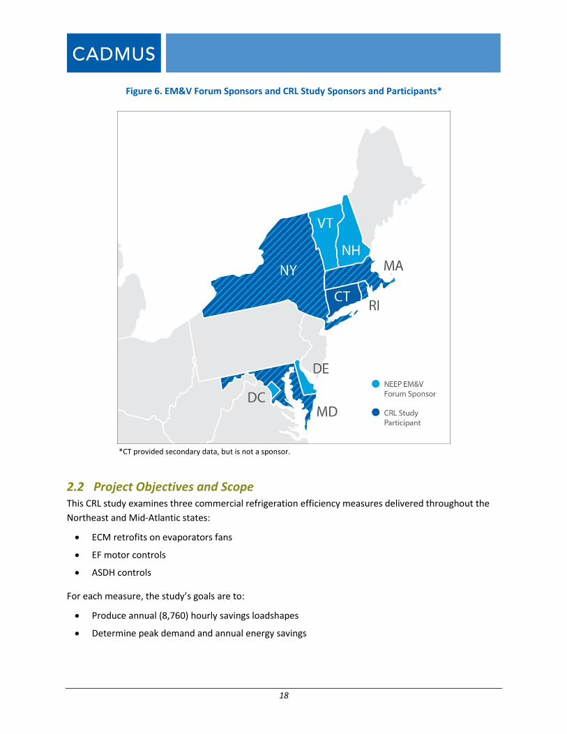
Figure 6 shows the EM&V Forum sponsors and indicates the states participating in this commercial
refrigeration loadshape project.
7 More information about the Northeast Energy Efficiency Partnership can be found at www.neep.org.
8 The NEEP EM&V forum has completed three loadshape studies to date: The Commercial Lighting Loadshape
Study (completed in 2011), the Unitary AC Loadshape Study (completed in 2012), and the VSD Loadshape
Study (completed in 2014).
18
Figure 6. EM&V Forum Sponsors and CRL Study Sponsors and Participants*
*CT provided secondary data, but is not a sponsor.
2.2 Project Objectives and Scope This CRL study examines three commercial refrigeration efficiency measures delivered throughout the
Northeast and Mid-Atlantic states:
ECM retrofits on evaporators fans
EF motor controls
ASDH controls
For each measure, the study’s goals are to:
Produce annual (8,760) hourly savings loadshapes
Determine peak demand and annual energy savings
19
Provide recommendations to improve prescriptive savings estimates, such as those described in
technical reference manuals (TRM)
The study uses both primary data—direct power metering and data collection for a sample of measure
installations across the sponsors’ programs—and secondary data from existing studies to establish the
hourly savings loadshapes for each of these selected measures.
2.3 Technology Review For each measure, the sections below describe the typical baseline and installed conditions and how the
measure saves energy.
2.3.1 ECM Retrofits
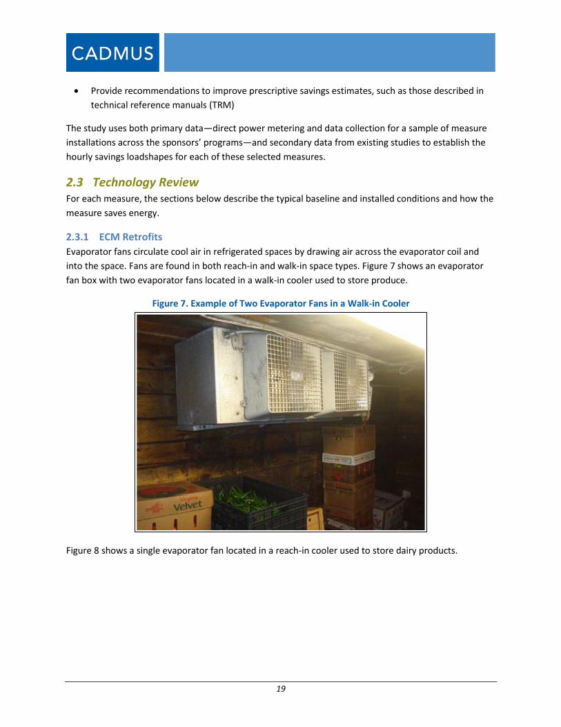
Evaporator fans circulate cool air in refrigerated spaces by drawing air across the evaporator coil and
into the space. Fans are found in both reach-in and walk-in space types. Figure 7 shows an evaporator
fan box with two evaporator fans located in a walk-in cooler used to store produce.
Figure 7. Example of Two Evaporator Fans in a Walk-in Cooler
Figure 8 shows a single evaporator fan located in a reach-in cooler used to store dairy products.
20
Figure 8. Example of Evaporator Fan in a Reach-in Cooler
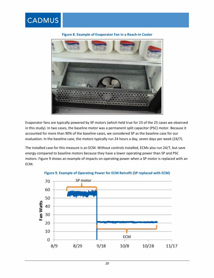
Evaporator fans are typically powered by SP motors (which held true for 23 of the 25 cases we observed
in this study). In two cases, the baseline motor was a permanent split capacitor (PSC) motor. Because it
accounted for more than 90% of the baseline cases, we considered SP as the baseline case for our
evaluation. In the baseline case, the motors typically run 24 hours a day, seven days per week (24/7).
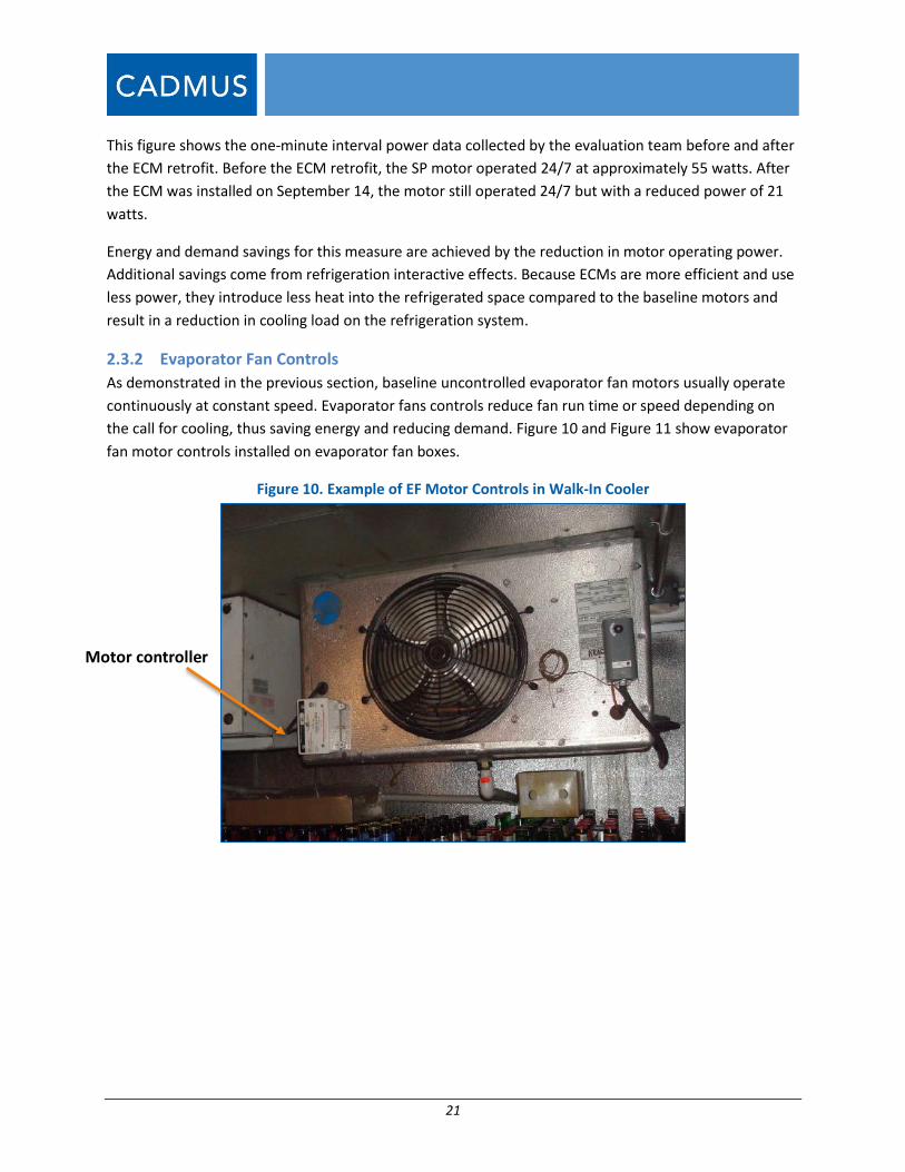
The installed case for this measure is an ECM. Without controls installed, ECMs also run 24/7, but save
energy compared to baseline motors because they have a lower operating power than SP and PSC
motors. Figure 9 shows an example of impacts on operating power when a SP motor is replaced with an
ECM.
Figure 9. Example of Operating Power for ECM Retrofit (SP replaced with ECM)
SP motor
ECM
21
This figure shows the one-minute interval power data collected by the evaluation team before and after
the ECM retrofit. Before the ECM retrofit, the SP motor operated 24/7 at approximately 55 watts. After
the ECM was installed on September 14, the motor still operated 24/7 but with a reduced power of 21
watts.
Energy and demand savings for this measure are achieved by the reduction in motor operating power.
Additional savings come from refrigeration interactive effects. Because ECMs are more efficient and use
less power, they introduce less heat into the refrigerated space compared to the baseline motors and
result in a reduction in cooling load on the refrigeration system.
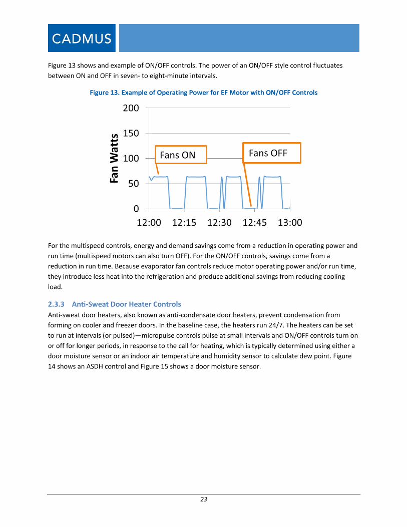
2.3.2 Evaporator Fan Controls
As demonstrated in the previous section, baseline uncontrolled evaporator fan motors usually operate
continuously at constant speed. Evaporator fans controls reduce fan run time or speed depending on
the call for cooling, thus saving energy and reducing demand. Figure 10 and Figure 11 show evaporator
fan motor controls installed on evaporator fan boxes.
Figure 10. Example of EF Motor Controls in Walk-In Cooler
Motor controller

22
Figure 11. Example of EF Controller for ECM
The evaluation team observed two types of evaporator fan controls:
Multispeed controls change the speed of the motors in response to the call for cooling.
ON/OFF controls turn the motors on and off in response to the call for cooling.
Figure 12 and Figure 13 shows examples of these two control methods. Both figures show one-minute
interval power data over a one-hour period.
Figure 12 shows an example of a fan power when operating with multispeed controls. The operating
power of a multispeed control fluctuates from high to low power at seven- to eight-minute intervals.
Figure 12. Example of Operating Power for EF Motor with Multispeed Controls
High speed Low speed
23
Figure 13 shows and example of ON/OFF controls. The power of an ON/OFF style control fluctuates
between ON and OFF in seven- to eight-minute intervals.
Figure 13. Example of Operating Power for EF Motor with ON/OFF Controls
For the multispeed controls, energy and demand savings come from a reduction in operating power and
run time (multispeed motors can also turn OFF). For the ON/OFF controls, savings come from a
reduction in run time. Because evaporator fan controls reduce motor operating power and/or run time,
they introduce less heat into the refrigeration and produce additional savings from reducing cooling
load.
2.3.3 Anti-Sweat Door Heater Controls
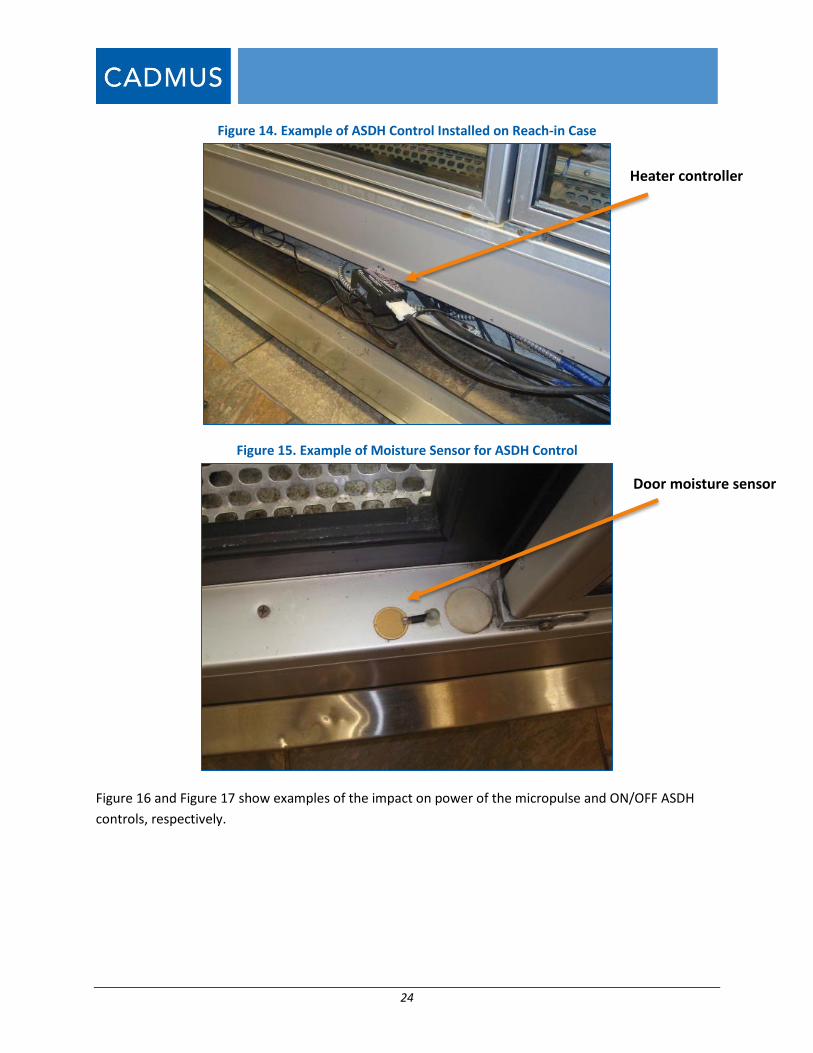
Anti-sweat door heaters, also known as anti-condensate door heaters, prevent condensation from
forming on cooler and freezer doors. In the baseline case, the heaters run 24/7. The heaters can be set
to run at intervals (or pulsed)—micropulse controls pulse at small intervals and ON/OFF controls turn on
or off for longer periods, in response to the call for heating, which is typically determined using either a
door moisture sensor or an indoor air temperature and humidity sensor to calculate dew point. Figure
14 shows an ASDH control and Figure 15 shows a door moisture sensor.
Fans ON Fans OFF
24
Figure 14. Example of ASDH Control Installed on Reach-in Case
Figure 15. Example of Moisture Sensor for ASDH Control
Figure 16 and Figure 17 show examples of the impact on power of the micropulse and ON/OFF ASDH
controls, respectively.
Heater controller
Door moisture sensor
25
Figure 16. Example of Operating Power for ASDH with Micropulse Controls
Figure 17. Example of Operating Power for ASDH with ON/OFF Controls
Figure 16 and Figure 17 show one-minute interval power data for ASDH controls over a one-hour period.
Micropulse controls pulse the door heaters for fractions of a second, in response to the call for heating.
Because Figure 16 shows the operating power at a one-minute interval resolution, the micro-reductions
in run time appear as a reduction in operating power. The ON/OFF controls turn the heaters on and off
for minutes at time, resulting in a reduction in run time. Both of these reductions result in energy and
demand savings. Additional savings come from refrigeration interactive effects. When the heaters run
less, they introduce less heat into the refrigeration system and reduce the cooling load.
26
3 Methods
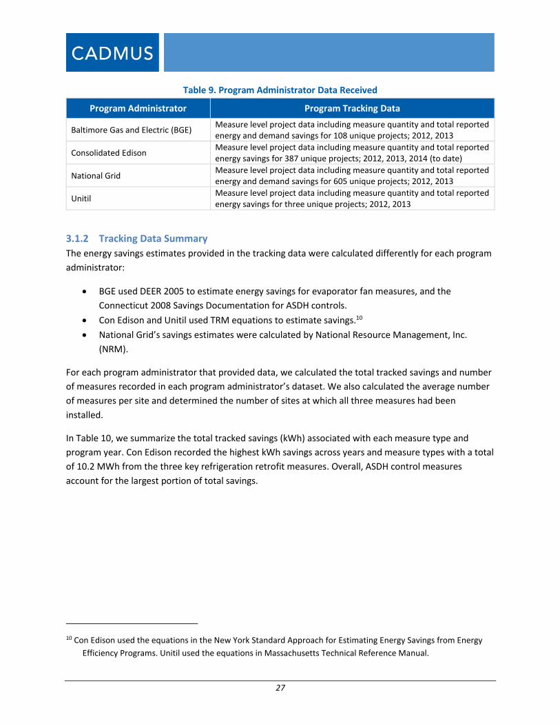
The evaluation team completed five key tasks, as listed in Figure 18. The progression of tasks for this CRL
study is similar to the previous loadshape studies and other EM&V research commissioned by NEEP. In
this section and the appendices, we describe the methods for each analysis task and our observations
and assumptions.
Figure 18. Key Tasks for Commercial Refrigeration Loadshape Analysis
3.1 Tracking Data Review The evaluation team asked participating program administrators (PAs) for the past two years of program
tracking data on prescriptive refrigeration equipment installations. These data showed the distribution
of projects across the program administrators’ service territories, the distribution of measures across
projects, and the tracked energy savings for each measure and each program administrator.
In this section, we summarize the project and measure level information contained in the data and
describe some of the key population characteristics that informed sample design and site visit planning.
3.1.1 Tracking Data Received
Table 9 lists the data received for each program administrator.9 These data were for ECM retrofits,
evaporator fan controls, and ASDH controls measures.
9 The evaluation team received program tracking data from Baltimore Gas and Electric, Con Edison, National
Grid, and Unitil. NYSEG indicated that few projects had installed the measures of interest, sothey were not
included in the sample.
Tracking Data Review
Secondary Data Review
Sample Design
Primary Data Collection
Data Analysis
27
Table 9. Program Administrator Data Received
Program Administrator Program Tracking Data
Baltimore Gas and Electric (BGE) Measure level project data including measure quantity and total reported energy and demand savings for 108 unique projects; 2012, 2013
Consolidated Edison Measure level project data including measure quantity and total reported energy savings for 387 unique projects; 2012, 2013, 2014 (to date)
National Grid Measure level project data including measure quantity and total reported energy and demand savings for 605 unique projects; 2012, 2013
Unitil Measure level project data including measure quantity and total reported energy savings for three unique projects; 2012, 2013
3.1.2 Tracking Data Summary
The energy savings estimates provided in the tracking data were calculated differently for each program
administrator:
BGE used DEER 2005 to estimate energy savings for evaporator fan measures, and the
Connecticut 2008 Savings Documentation for ASDH controls.
Con Edison and Unitil used TRM equations to estimate savings.10
National Grid’s savings estimates were calculated by National Resource Management, Inc.
(NRM).
For each program administrator that provided data, we calculated the total tracked savings and number
of measures recorded in each program administrator’s dataset. We also calculated the average number
of measures per site and determined the number of sites at which all three measures had been
installed.
In Table 10, we summarize the total tracked savings (kWh) associated with each measure type and
program year. Con Edison recorded the highest kWh savings across years and measure types with a total
of 10.2 MWh from the three key refrigeration retrofit measures. Overall, ASDH control measures
account for the largest portion of total savings.
10 Con Edison used the equations in the New York Standard Approach for Estimating Energy Savings from Energy
Efficiency Programs. Unitil used the equations in Massachusetts Technical Reference Manual.
28
Table 10. Total Tracked Savings (kWh) by Measure and PA
Year Program Administrator
Measure BGE Con Edison National Grid Unitil
2012
ECMs* 354,796 307,613 1,026,423 21,105
EF Controls 3,314 0 1,572,159 0
ASDH Controls 1,129,915 252,684 914,362 0
2013
ECMs* 35,356 2,314,800 971,952 11,793
EF Controls 0 1,389,484 1,767,443 0
ASDH Controls 239,417 5,896,582 1,005,357 0
Total
ECMs* 390,152 2,622,413 1,998,375 32,898
EF Controls 3,314 1,389,484 3,339,602 0
ASDH Controls 1,369,332 6,149,266 1,919,719 0
ALL 1,762,798 10,161,162 7,257,696 32,898
*ECM retrofits were specified for display cases and walk-in coolers in the Con Edison and National Grid datasets but not in the BGE dataset.
In Table 11, we summarize the total number of measures recorded within measure type. ECM retrofits
are the most common measure, appearing with the highest frequency across the program
administrators.
Table 11. Total Tracked Measures by Measure and PA
Year
Measure
Program Administrator
BGE Con Edison National Grid Unitil
2012
ECMs* 5,932 658 2,025 1
EF Controls 7 0 441 0
ASDH Controls 1,043 55 301 0
2013
ECMs* 628 4,282 1,904 2
EF Controls 0 809 515 0
ASDH Controls 221 1,983 344 0
Total
ECMs* 6,560 4,940 3,929 3
EF Controls 7 809 956 0
ASDH Controls 1,264 2,038 645 0
ALL 7,831 7,787 5,530 3
*ECM installations were specified distinctly for display cases and walk-in coolers in the Con Edison and National Grid datasets but not in the BGE dataset.
Table 12 provides the average per-unit kWh savings by program administrator.
29
Table 12. Average Tracked Unit Savings (kWh)
Measure Program Administrator*
BGE Con Edison National Grid
ECM Retrofit (Refrigerated Case) 59
330 249
ECM Retrofit (Walk-In Cooler/Freezer) 964 550
EF Controls 473 1,881 3,320
ASDH Controls 1,083 2,829 2,866
*Unit averages not reported for Unitil due to small total number of measures (3)
Note: Average per-unit savings data calculated as the total reported savings in the PA tracking
database divided by the total quantity of units in the PA tracking database.
BGE’s per-unit reported savings are lower than both Con Edison and National Grid for all measures.
National Grid reports the largest savings per unit for evaporator fan controls, but Con Edison claims the
highest savings for ECM retrofits. National Grid and Con Edison have nearly the same average savings
from ASDH control installations.
Table 13 lists the number of sites within each program administrator that contain one or more of the
measure types (combined across years). This gave us information on the number of measures we could
expect to meter at each sampled location and helped us plan our site visits. For example, at the 47 Con
Edison project sites, we could expect to meter units of all three types, whereas at all BGE sites, we could
expect to measure at most two types of measures. Note that although Con Edison has the highest
number of measures (as shown in Table 11), National Grid has the highest number of sites (605) overall
(as shown in Table 13). National Grid also has the highest number of sites that include all three measure
types (ECMs, evaporator fan controls, and ASDH controls).
Table 13. Number of Unique Measures Installed Per Site
Number of Unique Measures Installed
Program Administrator
BGE Con Edison National Grid Unitil
1 65 108 101 3
2 43 232 229 0
3 0 47 275 0
Total Number of Sites 108 387 605 3
Table 14 lists the average number of measures per site by measure type. Note that the average number
of measures per National Grid site was quite a bit lower than at either the BGE or Con Edison sites. BGE
had the highest number of ECMs and evaporator fan controls installed per site (67 on average) and Con
Edison had the highest number of ASDH controls installed per site.
30
Table 14. Average Number of Measures per Site
Measure Program Administrator*
BGE Con Edison National Grid
ECM Retrofit (Refrigerated Case) 64
32 20
ECM Retrofit (Walk-In Cooler/Freezer) 11 6
EF Controls 7 5 2
ASDH Controls 27 29 2
*Averages not reported for Unitil due to small total number of measures (3).
To understand the variation in savings within each program administrator, we calculated the coefficient
of variation for each measure type and program administrator. As shown in Table 15, for example,
there is greater variability in savings from National Grid’s ASDH controls than in National Grid’s savings
from ECM measures.
Table 15. CV of Unit Tracked Savings (kWh)
Measure Program Administrator**
BGE Con Edison National Grid
ECM Retrofit (Refrigerated Case) 0.436
1.599 0.208
ECM Retrofit (Walk-In Cooler/Freezer) 0.621 0.297
EF Controls N/A* 0.496 0.489
ASDH Controls 0.000 0.596 0.744
*Sample size too small to calculate standard deviation.
**Unit-level savings not reported for Unitil due to small total number of measures (3)
In addition to energy savings, BGE and National Grid datasets also recorded demand savings. Table 16
shows the average per-unit kW savings each reported. As with the recorded per-unit energy savings,
BGE’s reported per-unit demand savings were much lower than those reported by National Grid.
Table 16. Average Unit-Level Tracked Savings (kW)
Measure Program Administrator***
BGE Con Edison* National Grid**
ECM Retrofit (Refrigerated Case) 0.01
N/A 0.03
ECM Retrofit (Walk-In Cooler/Freezer) 0.10
EF Controls 0.06 N/A 0.32
ASDH Controls 0.02 N/A 0.16
*Savings in kW not reported **Values are based on Peak Diversified kW Reduction dataset values. ***Average unit-level savings not reported for Unitil due to small total number of measures (3)
Table 17 shows the coefficient of variation (CV) of the average per-unit demand savings recorded by BGE
and National Grid.
31
Table 17. CV of Average Unit Tracked kW Savings
Measure Program Administrator****
BGE Con Edison* National Grid**
ECM Retrofit (Refrigerated Case) 0.077
N/A 0.003
ECM Retrofit (Walk-In Cooler/Freezer) N/A 0.099
EF Controls N/A*** N/A 0.667
ASDH Controls 0.001 N/A 0.750
*Not reported **Used Reported Peak Diversified kW Reduction ***Sample size too small to calculate standard deviation ****Average unit-level savings not reported for Unitil due to small total number of measures (3)
3.1.3 Summary of Findings from Tracking Data Review
From our review of the tracking data, we determined that:
The 2012 and 2013 participation populations in BGE, Con Edison, and National Grid territories
provide a sufficient number of sites for post-installation metering. Other program administrators
may also have had sites available for sampling, but they did not have significant participation
levels.
Given the expectation of a small number of sample sites for metering, the project sampling plan
attempts to meter customer types that would be typically served by the sponsors.
The average tracked savings for each measure vary by program administrator. BGE reported the
lowest average savings by measure across all measures, National Grid reported the highest
average savings for evaporator fan control installations, and Con Edison reported the highest
savings for ECM installations. Con Edison and National Grid reported nearly identical average
savings for ASDH control installations.
Our review of the tracking data demonstrates that sponsors are reporting different savings for nearly
identical measure installations. The study therefore does not attempt to create a sample representing
the populations based on reported energy savings.
3.2 Secondary Data Review The team collected secondary data—including reports and raw metering data from previous evaluation
studies—to design the sampling plan and supplement the primary data collection. This section discusses
the secondary data records collected and how they were useful in shaping project analysis and overall
approach.
We used secondary data in two ways. First, to establish the sampling approach and metering protocols
for the overall analysis plan, we collected and analyzed available secondary data from completed
evaluations, technology assessments, and TRMs from the Northeast and Mid-Atlantic. Our review
32
confirmed or determined the following operating parameters and the variability in performance across
measure installations (to inform the sampling plan):
Evaporator fan motors and door heaters without controls operate nearly continuously (24/7).
Door heater control operation does not vary with outside temperatures, so data collection can be
short and at any time of year.
Although technology performance may not vary by location, implementers use different
equipment models in each region, so it is important to capture data in several regions.
There are limited baseline power measurements available, which suggests the existing TRM
savings estimates are based on assumptions and not baseline equipment measurements.
Second, to create a more robust sample, we added any secondary metered data that met the minimum
data collection requirements (e.g., metering duration) to the primary dataset. This secondary data
research contributed to preparing a more effective evaluation plan, reducing the required evaluation
sample, shortening the expected data collection period, and reducing evaluation costs.
We worked with the NEEP project coordinator to request metering data from four commercial
refrigeration utility program evaluators. Table 18 shows these vendors and the states in which the
secondary data were recorded.
Table 18. Metering Data Received
Vendors State
Michaels/EMI CT
KEMA/DNV-GL CT, MA
DMI MA
See Appendix A. Secondary Data Review for complete descriptions of the secondary data including
sources, type, and value to the study.
3.3 Sample Design The team designed the evaluation sample for primary data collection to include sites that offer pre-
retrofit baseline case (projects that are in the pipeline but had not yet been installed) and installed case
(projects that had been installed) metering. Site visits took place in BGE territory in Maryland where
measures were installed by NRM, Anthony International, and Johnson Controls; National Grid territory
in Massachusetts and Rhode Island with measures installed by NRM; and Con Edison territory in New
York with measures installed by Global Energy Efficiency (GEE) and Willdan.11 12 The team worked with
11 There was one site in Maryland where the installer is unknown.
12 Data collection is limited to the territories of the program administrators that provided tracking data and has
significantly large populations from which to sample.
33
program vendors to identify customers eligible for baseline metering. The team used a random sample,
stratified by PA, to identify customers for post-installation metering.
Table 19 and Table 20 show the overall final sample for primary data collection (in number of unique
sites) by subcontractor and building type, respectively.
Table 19. Final Site Sample by Implementer (Primary Data)
Implementer Unique Sites MD
(BGE)
MA / RI
(National Grid)
NY
(Con Edison)
NRM 18 3 15 0
GEE 11 0 0 11
Anthony International 2 2 0 0
Johnson Controls 6 6 0 0
Unknown 1 1 0 0
Willdan 2 0 0 2
Total 40 12 15 13
The majority of sampled projects (29 of 40) were completed by NRM and GEE. NRM is the exclusive
large volume implementer for the small business projects in Massachusetts and Rhode Island and also
operates in Maryland. GEE installs most refrigeration projects for Con Edison in New York, as a
subcontractor to Willdan (which also installs some projects).
Table 20 shows the final sample by building type.
Table 20. Final Sample by Building Type
Building Type Count of Sites
Small Retail 35
Restaurant 3
Other 1
Large Retail 1
Total 40
The majority of installations were in small retail facilities, such as liquor stores, convenience stores,
delis, and pharmacies. There were several small chain restaurants, one nursing home (categorized as
“Other”), and one large retail facility.
In addition to the 40 total unique sites for primary data, we collected secondary data from an additional
19 unique sites. Since many refrigeration projects include a combination of the three retrofit measures,
we collected data on all three measures at many sites.
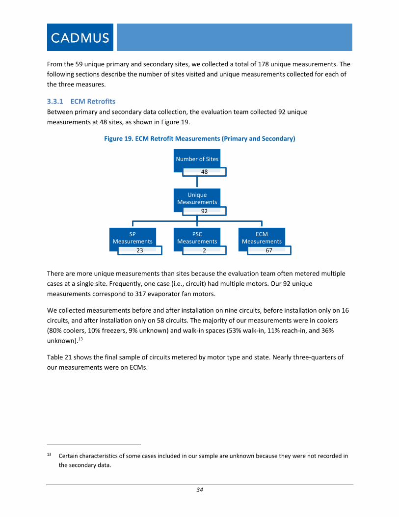
34
From the 59 unique primary and secondary sites, we collected a total of 178 unique measurements. The
following sections describe the number of sites visited and unique measurements collected for each of
the three measures.
3.3.1 ECM Retrofits
Between primary and secondary data collection, the evaluation team collected 92 unique
measurements at 48 sites, as shown in Figure 19.
Figure 19. ECM Retrofit Measurements (Primary and Secondary)
There are more unique measurements than sites because the evaluation team often metered multiple
cases at a single site. Frequently, one case (i.e., circuit) had multiple motors. Our 92 unique
measurements correspond to 317 evaporator fan motors.
We collected measurements before and after installation on nine circuits, before installation only on 16
circuits, and after installation only on 58 circuits. The majority of our measurements were in coolers
(80% coolers, 10% freezers, 9% unknown) and walk-in spaces (53% walk-in, 11% reach-in, and 36%
unknown).13
Table 21 shows the final sample of circuits metered by motor type and state. Nearly three-quarters of
our measurements were on ECMs.
13 Certain characteristics of some cases included in our sample are unknown because they were not recorded in
the secondary data.
Number of Sites
48
Unique Measurements
92
SP Measurements
23
PSC Measurements
2
ECM Measurements
67
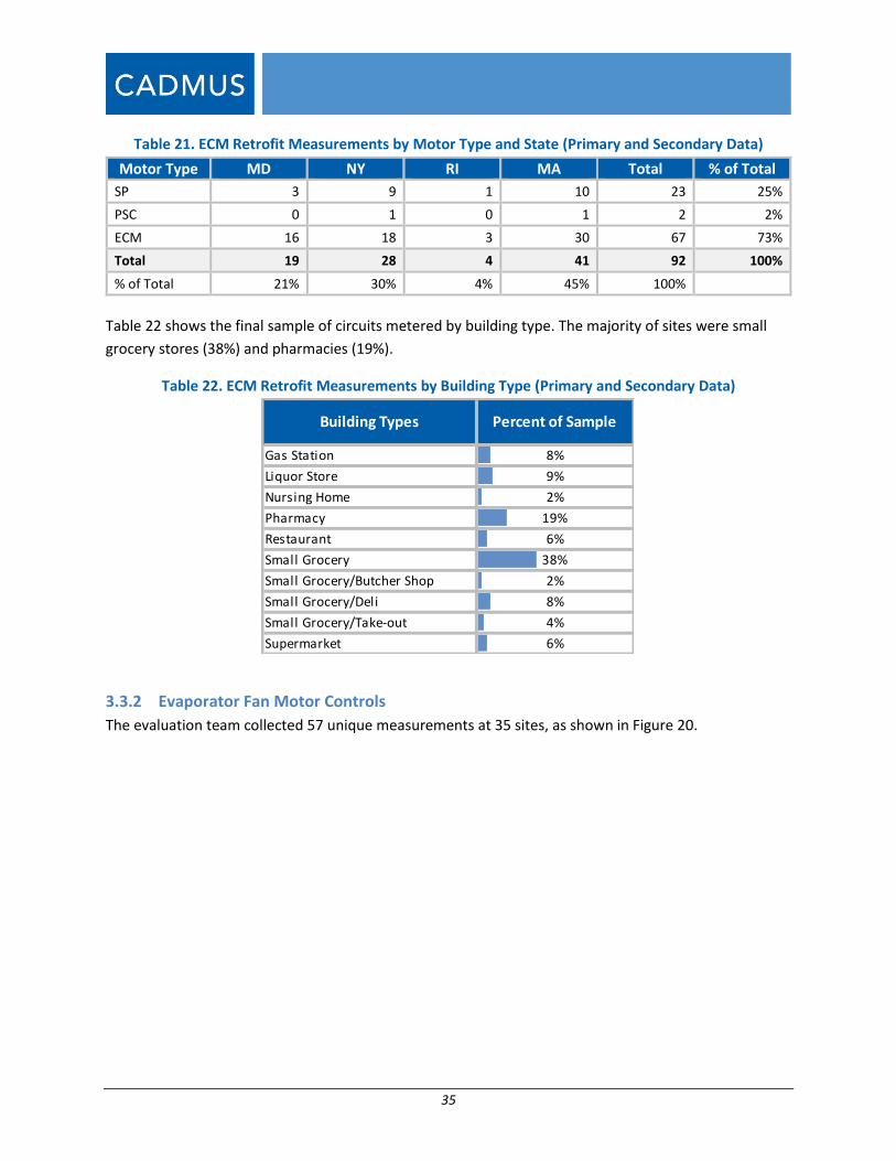
35
Table 21. ECM Retrofit Measurements by Motor Type and State (Primary and Secondary Data)
Motor Type MD NY RI MA Total % of Total
SP 3 9 1 10 23 25%
PSC 0 1 0 1 2 2%
ECM 16 18 3 30 67 73%
Total 19 28 4 41 92 100%
% of Total 21% 30% 4% 45% 100%
Table 22 shows the final sample of circuits metered by building type. The majority of sites were small
grocery stores (38%) and pharmacies (19%).
Table 22. ECM Retrofit Measurements by Building Type (Primary and Secondary Data)
3.3.2 Evaporator Fan Motor Controls
The evaluation team collected 57 unique measurements at 35 sites, as shown in Figure 20.
9%
2%
19%
Building Types
8%
4%
6%
Gas Station
Liquor Store
Nursing Home
Pharmacy
Restaurant
Small Grocery
Small Grocery/Butcher Shop
Small Grocery/Deli
Small Grocery/Take-out
Supermarket
6%
38%
2%
Percent of Sample
8%
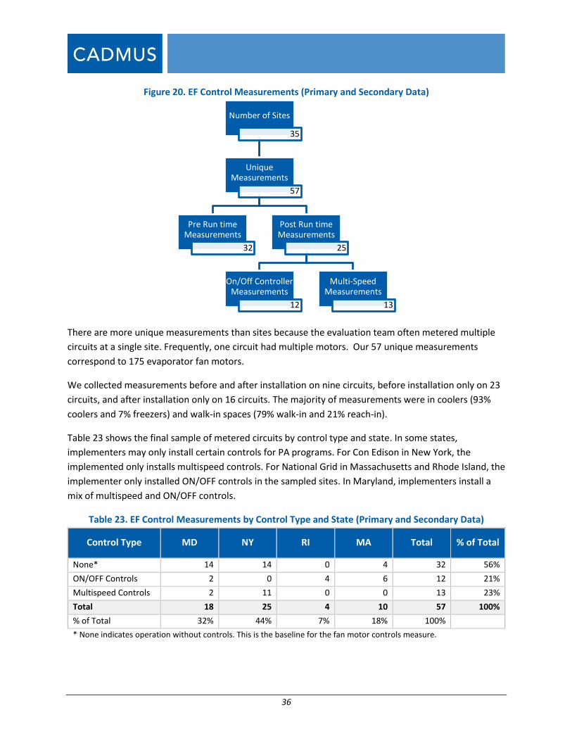
36
Figure 20. EF Control Measurements (Primary and Secondary Data)
There are more unique measurements than sites because the evaluation team often metered multiple
circuits at a single site. Frequently, one circuit had multiple motors. Our 57 unique measurements
correspond to 175 evaporator fan motors.
We collected measurements before and after installation on nine circuits, before installation only on 23
circuits, and after installation only on 16 circuits. The majority of measurements were in coolers (93%
coolers and 7% freezers) and walk-in spaces (79% walk-in and 21% reach-in).
Table 23 shows the final sample of metered circuits by control type and state. In some states,
implementers may only install certain controls for PA programs. For Con Edison in New York, the
implemented only installs multispeed controls. For National Grid in Massachusetts and Rhode Island, the
implementer only installed ON/OFF controls in the sampled sites. In Maryland, implementers install a
mix of multispeed and ON/OFF controls.
Table 23. EF Control Measurements by Control Type and State (Primary and Secondary Data)
Control Type MD NY RI MA Total % of Total
None* 14 14 0 4 32 56%
ON/OFF Controls 2 0 4 6 12 21%
Multispeed Controls 2 11 0 0 13 23%
Total 18 25 4 10 57 100%
% of Total 32% 44% 7% 18% 100%
* None indicates operation without controls. This is the baseline for the fan motor controls measure.
Number of Sites
35
Unique Measurements
57
Pre Run time Measurements
32
Post Run time Measurements
25
On/Off Controller Measurements
12
Multi-Speed Measurements
13

37
Table 24 shows the final sample of circuits metered by building type for evaporator fan controls. The
majority of sites were small grocery stores (39%) and pharmacies (18%).
Table 24. EF Control Measurements by Building Type (Primary and Secondary Data)
3.3.3 Anti-Sweat Door Heater Controls
We collected 29 unique ASDH measurements at 22 sites, as shown in Figure 21.
Figure 21. ASDH Measurements (Primary and Secondary Data)
There are more unique ASDH measurements than sites because the evaluation team often metered
multiple case circuits at a single site. Our 29 measurements, which each correspond to a single
controller that control a group of doors, correspond to 240 doors.
Building Types Percent of Sample
Gas Station 11%
Liquor Store 9%
Nursing Home 2%
Pharmacy 18%
Restaurant 5%
Small Grocery 39%
Supermarket 5%
Small Grocery/Butcher Shop 2%
Small Grocery/Deli 5%
Small Grocery/Take-out 5%
Number of Sites
22
Unique Measurements
29
Pre Run time Measurements
10
Post Run time Measurements
19
On/Off Controller Controllers
6
MicropulseControllers
6
Unknown Controllers
7
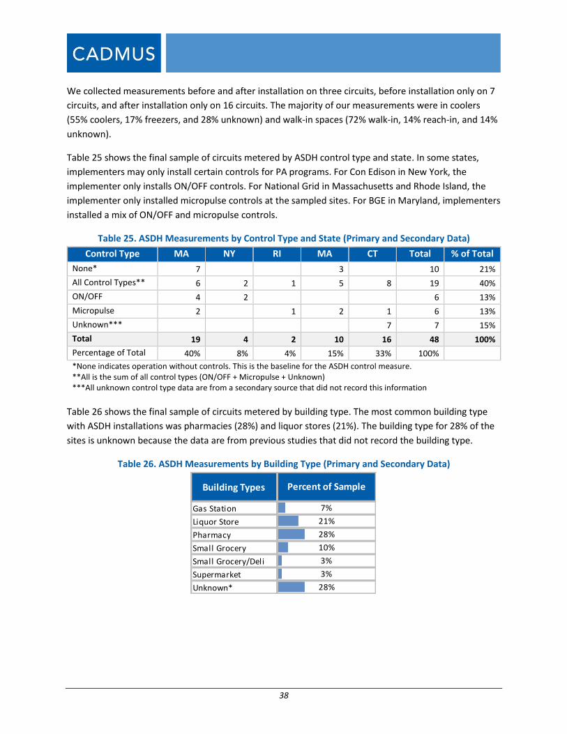
38
We collected measurements before and after installation on three circuits, before installation only on 7
circuits, and after installation only on 16 circuits. The majority of our measurements were in coolers
(55% coolers, 17% freezers, and 28% unknown) and walk-in spaces (72% walk-in, 14% reach-in, and 14%
unknown).
Table 25 shows the final sample of circuits metered by ASDH control type and state. In some states,
implementers may only install certain controls for PA programs. For Con Edison in New York, the
implementer only installs ON/OFF controls. For National Grid in Massachusetts and Rhode Island, the
implementer only installed micropulse controls at the sampled sites. For BGE in Maryland, implementers
installed a mix of ON/OFF and micropulse controls.
Table 25. ASDH Measurements by Control Type and State (Primary and Secondary Data)
Control Type MA NY RI MA CT Total % of Total
None* 7 3 10 21%
All Control Types** 6 2 1 5 8 19 40%
ON/OFF 4 2 6 13%
Micropulse 2 1 2 1 6 13%
Unknown*** 7 7 15%
Total 19 4 2 10 16 48 100%
Percentage of Total 40% 8% 4% 15% 33% 100%
*None indicates operation without controls. This is the baseline for the ASDH control measure. **All is the sum of all control types (ON/OFF + Micropulse + Unknown) ***All unknown control type data are from a secondary source that did not record this information
Table 26 shows the final sample of circuits metered by building type. The most common building type
with ASDH installations was pharmacies (28%) and liquor stores (21%). The building type for 28% of the
sites is unknown because the data are from previous studies that did not record the building type.
Table 26. ASDH Measurements by Building Type (Primary and Secondary Data)
Building Types
Gas Station
Liquor Store
Pharmacy
Small Grocery
Small Grocery/Deli
Supermarket
Unknown*
7%
21%
28%
10%
3%
3%
28%
Percent of Sample
39
3.3.4 Sample Recruitment for Baseline Data
For baseline metering, the evaluation team worked with program implementation contractors
(implementers) to recruit participants:
For Massachusetts and Rhode Island, we worked with National Resource Management, Inc. (NRM)
to identify and schedule seven baseline sites.
In New York, we worked with Willdan Energy Services to identify and schedule five baseline sites.
In Maryland, NRM scheduled three baseline sites. We contacted five additional BGE program
contractors to identify more baseline sites. Two contractors reported they had no upcoming
retrofits, and we did not receive responses from the other three.
To maximize participation rates and minimize participation bias, we offered gift cards totaling $100 to
baseline participants ($50 gift card at the time of meter installation and $50 gift card at the time of
meter removal).
3.3.4.1 Selection Bias
Collecting baseline data requires that the evaluator access the equipment before the customer
implements the energy-efficient measure. However, because the implementer is responsible for most
implementation activities, it could select customers, sites, or projects that are likely to have the best
measure performance, for example, poor baseline performance (to demonstrate large improvement),
higher load or operating hours (to maximize savings potential), or customers most likely to optimize or
sustain measure performance.
Programs with measures that vary across customer sites (e.g., custom programs) or that perform
differently depending on the customer (e.g., lighting controls) are more vulnerable to this selection bias.
To minimize this risk of this bias, the evaluation team coordinated with the implementer and the
program administrator.
The evaluation team coordinated directly with the implementer in each state to identify any eligible
customer sites that could delay having the measure installed by at least two weeks to allow for sufficient
baseline metering. For convenience and to minimize customer burden, the implementer recruited the
sites for inspection and metering and scheduled all baseline visits. We understood this exposed the
sample to selection bias but made this choice because we anticipated little variation in measure
performance across customer sites (based on our secondary data review) and, therefore, low risk of
selection bias on the study results.
3.3.4.2 Performance Bias
Any pre-installation evaluation activities may introduce performance bias in the overall program and
measure performance; however, performance bias is not a concern in this study, due to the nature of
the measures. When evaluating measures that depend heavily on the customer interaction,

40
performance bias is of concern because the implementer may be more diligent with installation or the
customer may be more attentive to proper operation of the measure. However, the simplicity of
measure installation and the limited opportunity of the customer to influence measure performance
reduced the concerns for these sources of bias. For all three refrigeration measures, installation is
relatively simple—it either works or it does not—so the implementer or customer has little influence on
the measure performance. The ECM retrofit measure is a straightforward equipment replacement with
little variation in the selected make/model of the new equipment. For motor and door heater controls,
the implementer installs and connects a control box on the existing equipment, typically using the same
make and model of control equipment on all installations; controls typically require a one-time setup
with no future interaction by the contractor or customer.
3.3.5 Sample Recruitment for Post-Installation Data
For post-installation metering, the evaluation team randomly sampled participants from PA tracking
data showing customers who installed the three commercial refrigeration measures. Although we
designed the sample to not require collecting post-installation data only from baseline sites, we worked
with implementers in each state to maximize the amount of post-installation data we could collect at
sites where we also collected baseline data. Our final sample includes nine sites where we were able to
collect both baseline and post-installation data.
Similar to the baseline metering, to maximize participation rates and minimize participation bias, we
offered gift cards totaling $100 to baseline participants ($50 gift card at the time of meter installation
and $50 gift card at the time of meter removal).
3.4 Primary Data Collection The evaluation team collected primary data at 40 sites through on-site inspection and metering of key
equipment. We completed all on-site metering over a 3-4 month period from August 12 to December
17, 2014.
Figure 22 shows the duration of pre- and post-installation metering for each site. The pink bars indicate
baseline metering and the light green bars indicate post-installation metering. For sites in the baseline
sample, we collected a minimum of one week of data. For sites in the post-installation sample, we
collected a minimum of two weeks of post-installation data. On average, we collected five weeks of pre-
and seven weeks of post-installation data.
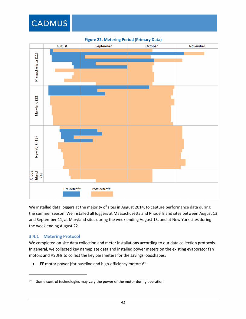
41
Figure 22. Metering Period (Primary Data)
We installed data loggers at the majority of sites in August 2014, to capture performance data during
the summer season. We installed all loggers at Massachusetts and Rhode Island sites between August 13
and September 11, at Maryland sites during the week ending August 15, and at New York sites during
the week ending August 22.
3.4.1 Metering Protocol
We completed on-site data collection and meter installations according to our data collection protocols.
In general, we collected key nameplate data and installed power meters on the existing evaporator fan
motors and ASDHs to collect the key parameters for the savings loadshapes:
EF motor power (for baseline and high-efficiency motors)14
14 Some control technologies may vary the power of the motor during operation.
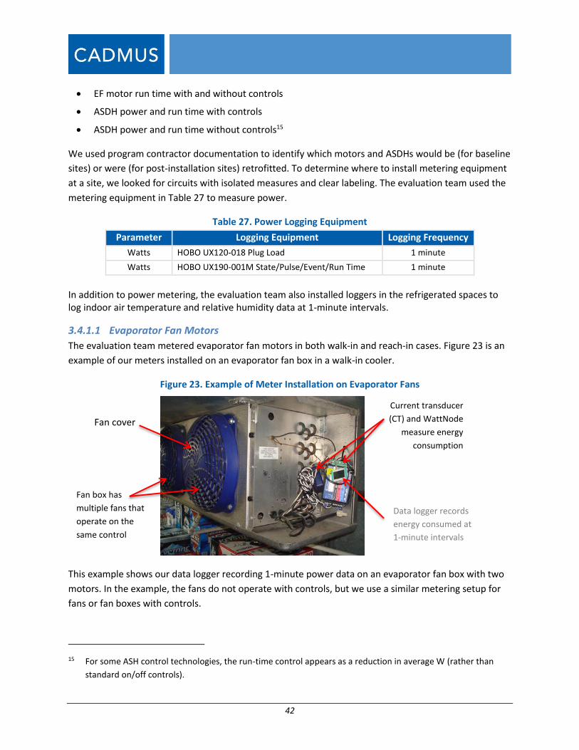
42
EF motor run time with and without controls
ASDH power and run time with controls
ASDH power and run time without controls15
We used program contractor documentation to identify which motors and ASDHs would be (for baseline
sites) or were (for post-installation sites) retrofitted. To determine where to install metering equipment
at a site, we looked for circuits with isolated measures and clear labeling. The evaluation team used the
metering equipment in Table 27 to measure power.
Table 27. Power Logging Equipment
Parameter Logging Equipment Logging Frequency
Watts HOBO UX120-018 Plug Load 1 minute
Watts HOBO UX190-001M State/Pulse/Event/Run Time 1 minute
In addition to power metering, the evaluation team also installed loggers in the refrigerated spaces to log indoor air temperature and relative humidity data at 1-minute intervals.
3.4.1.1 Evaporator Fan Motors
The evaluation team metered evaporator fan motors in both walk-in and reach-in cases. Figure 23 is an
example of our meters installed on an evaporator fan box in a walk-in cooler.
Figure 23. Example of Meter Installation on Evaporator Fans
This example shows our data logger recording 1-minute power data on an evaporator fan box with two
motors. In the example, the fans do not operate with controls, but we use a similar metering setup for
fans or fan boxes with controls.
15 For some ASH control technologies, the run-time control appears as a reduction in average W (rather than
standard on/off controls).
Fan cover
Fan box has
multiple fans that
operate on the
same control
Current transducer
(CT) and WattNode
measure energy
consumption
Data logger records
energy consumed at
5-minute intervals
Data logger records
energy consumed at
1-minute intervals
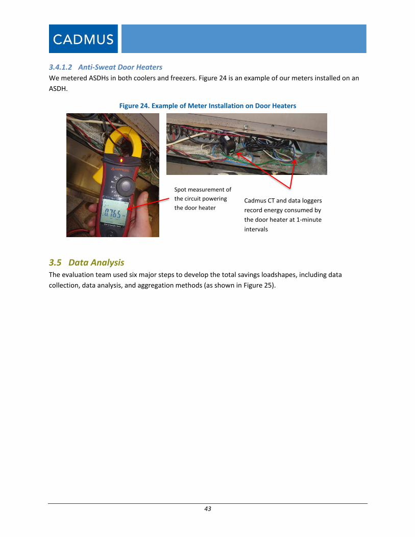
43
3.4.1.2 Anti-Sweat Door Heaters
We metered ASDHs in both coolers and freezers. Figure 24 is an example of our meters installed on an
ASDH.
Figure 24. Example of Meter Installation on Door Heaters
3.5 Data Analysis The evaluation team used six major steps to develop the total savings loadshapes, including data
collection, data analysis, and aggregation methods (as shown in Figure 25).
Spot measurement of
the circuit powering
the door heater Cadmus CT and data logger
record energy consumed
by the door heater at 5-
minute intervals.
Cadmus CT and data loggers
record energy consumed by
the door heater at 1-minute
intervals
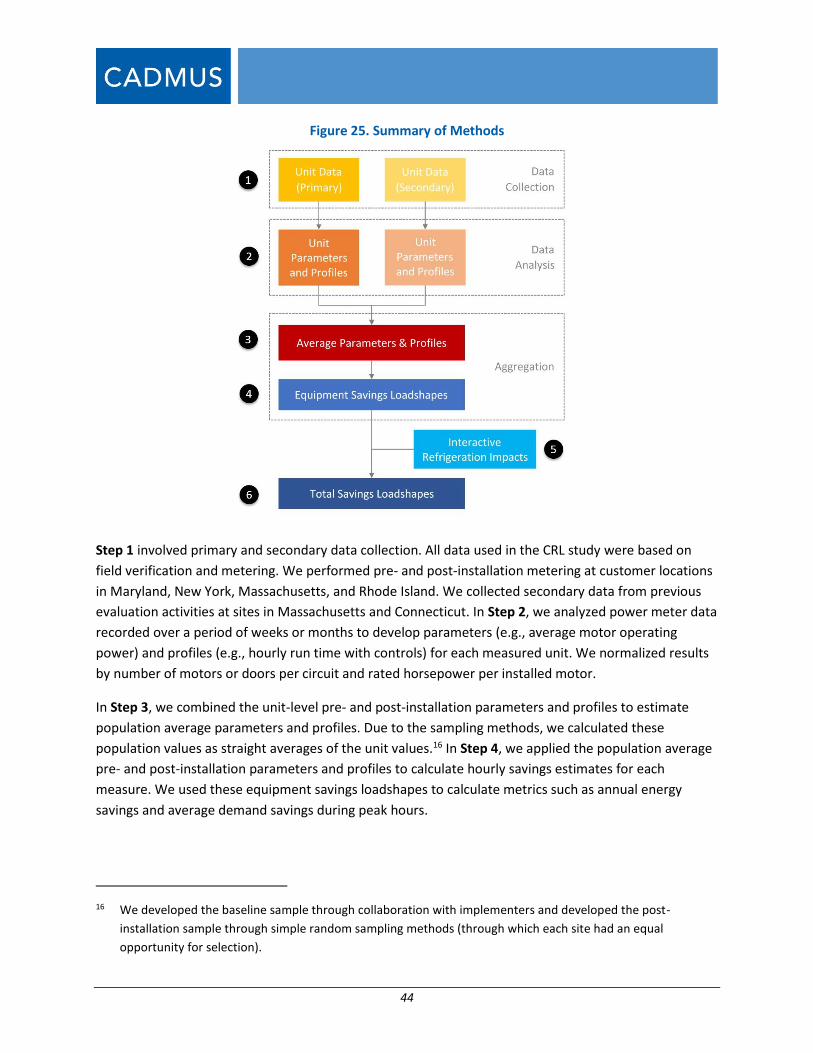
44
Figure 25. Summary of Methods
Step 1 involved primary and secondary data collection. All data used in the CRL study were based on
field verification and metering. We performed pre- and post-installation metering at customer locations
in Maryland, New York, Massachusetts, and Rhode Island. We collected secondary data from previous
evaluation activities at sites in Massachusetts and Connecticut. In Step 2, we analyzed power meter data
recorded over a period of weeks or months to develop parameters (e.g., average motor operating
power) and profiles (e.g., hourly run time with controls) for each measured unit. We normalized results
by number of motors or doors per circuit and rated horsepower per installed motor.
In Step 3, we combined the unit-level pre- and post-installation parameters and profiles to estimate
population average parameters and profiles. Due to the sampling methods, we calculated these
population values as straight averages of the unit values.16 In Step 4, we applied the population average
pre- and post-installation parameters and profiles to calculate hourly savings estimates for each
measure. We used these equipment savings loadshapes to calculate metrics such as annual energy
savings and average demand savings during peak hours.
16 We developed the baseline sample through collaboration with implementers and developed the post-
installation sample through simple random sampling methods (through which each site had an equal
opportunity for selection).
45
In Step 5, we developed the model to estimate the refrigeration interactive effects of the equipment
retrofit on refrigeration system loads and power. These effects result in additional savings due to the
reduced heat rejection requirements on the refrigeration system.
Finally, in Step 6, we applied the refrigeration interactive effects model to the equipment savings
loadshapes to calculate the total savings loadshapes. The total savings loadshapes represent the
combined impacts of the equipment retrofit and reduced refrigeration load. We separated Step 5 and
Step 6 from Step 4 to distinguish between savings from the equipment retrofit and saving due to
interactive load reduction on the refrigeration systems. Most TRMs use a similar approach to apply
these interactive effects as a multiplier on the equipment savings.
3.5.1 Unit Parameters and Profiles
To estimate savings for evaporator fan motors and ASDHs, the evaluation team used primary and
secondary data to assess key parameters (single values) and profiles (hourly values based on time of day
and day of week). The average full load operating power is a key parameter to determine the power
draw of motors and doors. The effective hourly run-time profiles provide hourly estimates of the
operating status of equipment with or without controls.
The next sections describe our approach to estimating these parameters and profiles.
3.5.1.1 Average Full Load Operating Power
We evaluated average hourly pre- and post-installation operating power for evaporator fan motors and
ASDHs by collecting one-minute interval power readings from each sampled unit. The meter data
showed three modes of operation:
ON, during which the motor/heater is running at full power for the entire minute interval
OFF, during which the motor/heater is off
State change, during which the motor/heater is either running at partial power or is turned ON or
OFF within the one-minute interval
Figure 26 shows power data from one evaporator fan motor with controls and identifies the three
modes of operation.
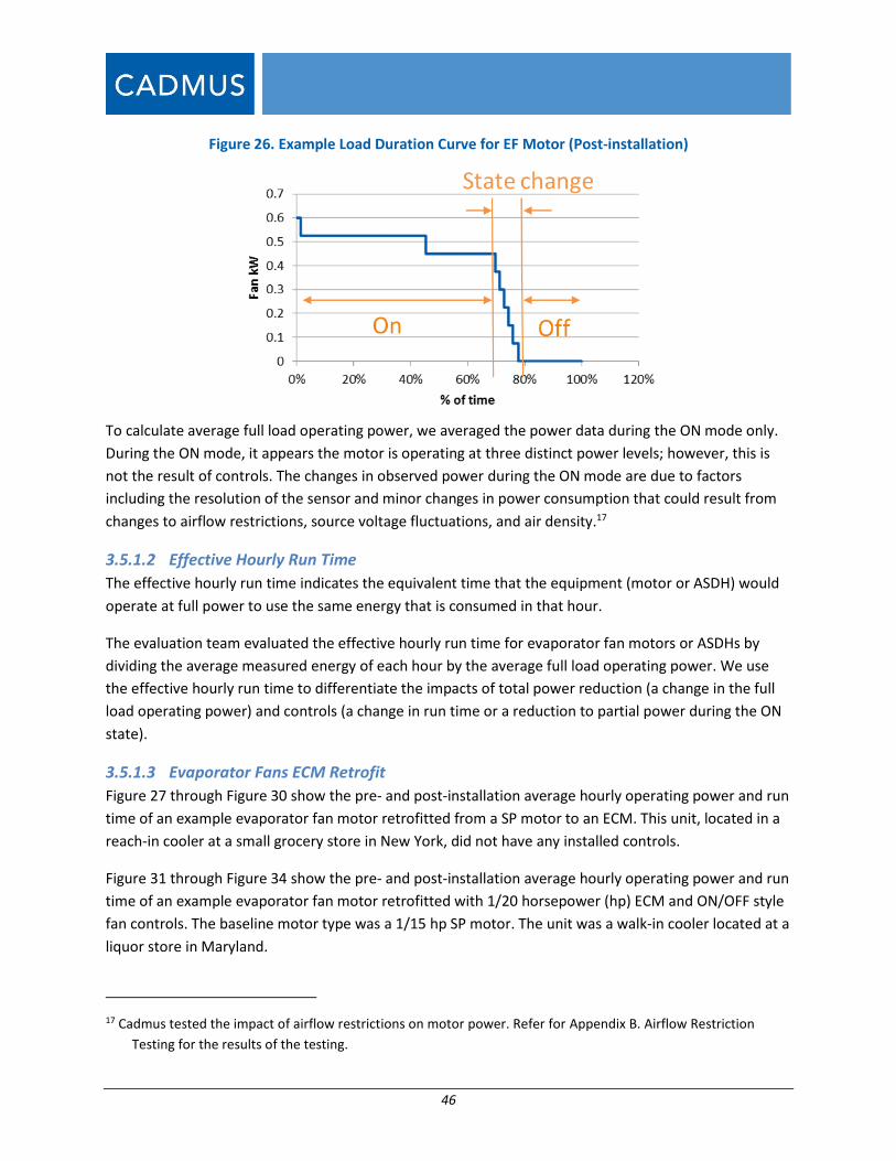
46
Figure 26. Example Load Duration Curve for EF Motor (Post-installation)
To calculate average full load operating power, we averaged the power data during the ON mode only.
During the ON mode, it appears the motor is operating at three distinct power levels; however, this is
not the result of controls. The changes in observed power during the ON mode are due to factors
including the resolution of the sensor and minor changes in power consumption that could result from
changes to airflow restrictions, source voltage fluctuations, and air density.17
3.5.1.2 Effective Hourly Run Time
The effective hourly run time indicates the equivalent time that the equipment (motor or ASDH) would
operate at full power to use the same energy that is consumed in that hour.
The evaluation team evaluated the effective hourly run time for evaporator fan motors or ASDHs by
dividing the average measured energy of each hour by the average full load operating power. We use
the effective hourly run time to differentiate the impacts of total power reduction (a change in the full
load operating power) and controls (a change in run time or a reduction to partial power during the ON
state).
3.5.1.3 Evaporator Fans ECM Retrofit
Figure 27 through Figure 30 show the pre- and post-installation average hourly operating power and run
time of an example evaporator fan motor retrofitted from a SP motor to an ECM. This unit, located in a
reach-in cooler at a small grocery store in New York, did not have any installed controls.
Figure 31 through Figure 34 show the pre- and post-installation average hourly operating power and run
time of an example evaporator fan motor retrofitted with 1/20 horsepower (hp) ECM and ON/OFF style
fan controls. The baseline motor type was a 1/15 hp SP motor. The unit was a walk-in cooler located at a
liquor store in Maryland.
17 Cadmus tested the impact of airflow restrictions on motor power. Refer for Appendix B. Airflow Restriction
Testing for the results of the testing.
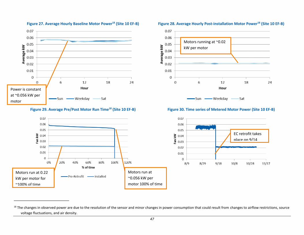
47
Figure 27. Average Hourly Baseline Motor Power18 (Site 10 EF-B) Figure 28. Average Hourly Post-installation Motor Power18 (Site 10 EF-B)
Figure 29. Average Pre/Post Motor Run Time18 (Site 10 EF-B) Figure 30. Time series of Metered Motor Power (Site 10 EF-B)
18 The changes in observed power are due to the resolution of the sensor and minor changes in power consumption that could result from changes to airflow restrictions, source
voltage fluctuations, and air density.
Motors running at ~0.02
kW per motor
Motors run at 0.22
kW per motor for
~100% of time
Power is constant
at ~0.056 kW per
motor
Motors run at
~0.056 kW per
motor 100% of time
EC retrofit takes
place on 9/14
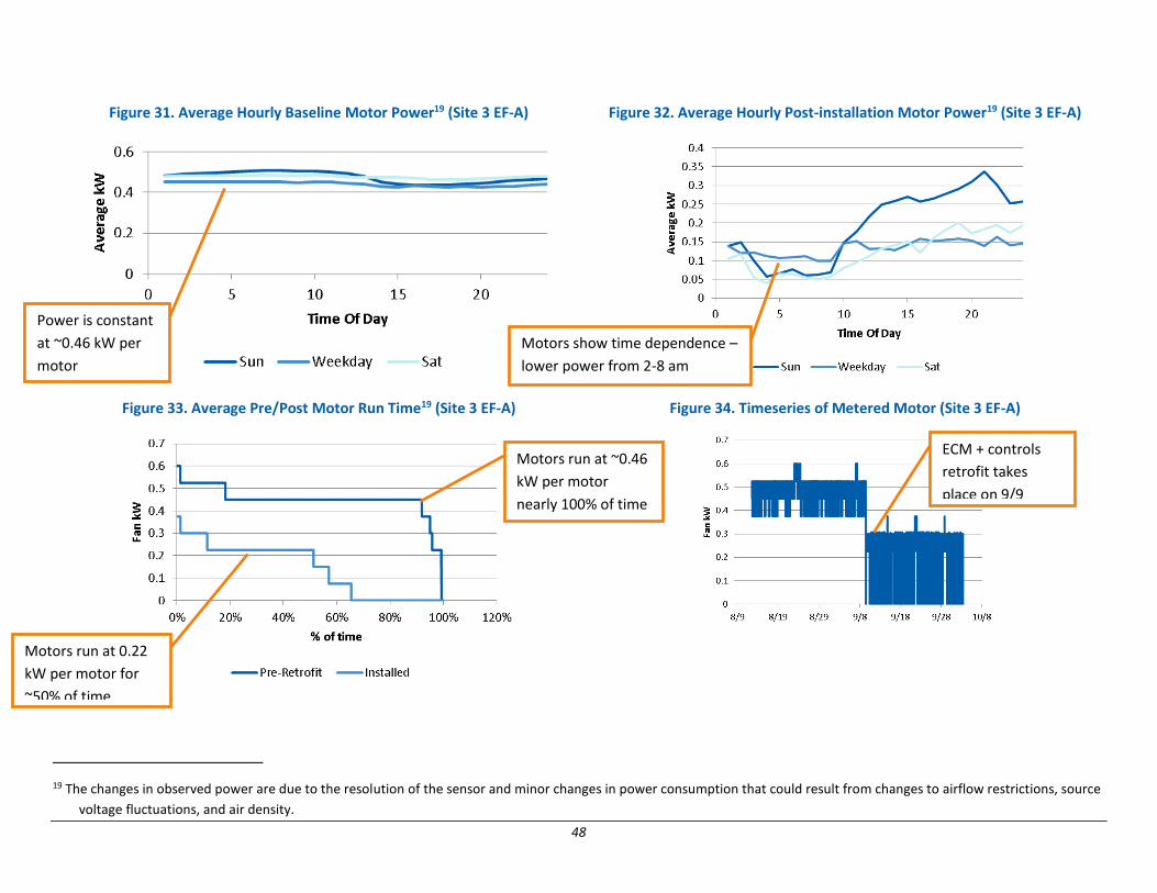
48
Figure 31. Average Hourly Baseline Motor Power19 (Site 3 EF-A) Figure 32. Average Hourly Post-installation Motor Power19 (Site 3 EF-A)
Figure 33. Average Pre/Post Motor Run Time19 (Site 3 EF-A) Figure 34. Timeseries of Metered Motor (Site 3 EF-A)
19 The changes in observed power are due to the resolution of the sensor and minor changes in power consumption that could result from changes to airflow restrictions, source
voltage fluctuations, and air density.
Power is constant
at ~0.46 kW per
motor
Motors run at ~0.46
kW per motor
nearly 100% of time
Motors run at 0.22
kW per motor for
~50% of time
ECM + controls
retrofit takes
place on 9/9
Motors show time dependence –
lower power from 2-8 am
49
3.5.1.4 Anti-Sweat Door Heater Controls
Figure 35 through Figure 38 show the pre- and post-installation average hourly operating power of an example ASDH retrofitted with micropulse style controls.
This control operates by automatically calculating the dew point in the store and applying just enough heat to doors to prevent sweating. The unit was located in
a walk-in cooler at a gas station in Massachusetts.
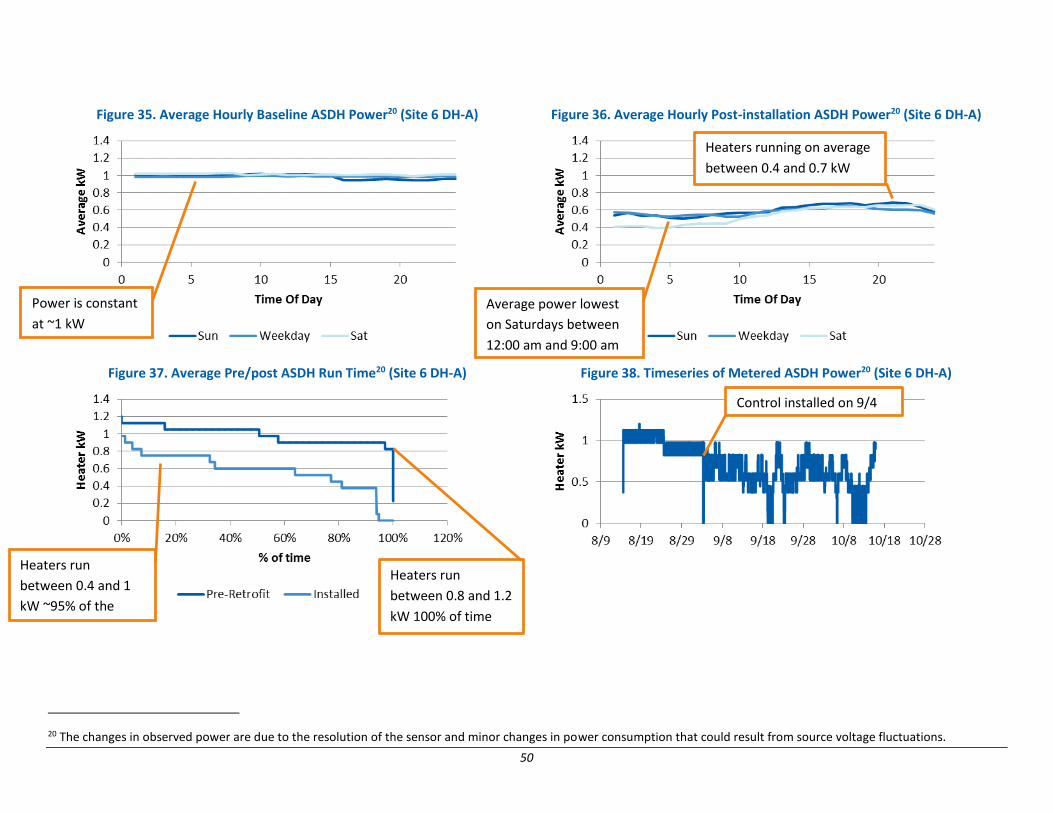
50
Figure 35. Average Hourly Baseline ASDH Power20 (Site 6 DH-A) Figure 36. Average Hourly Post-installation ASDH Power20 (Site 6 DH-A)
Figure 37. Average Pre/post ASDH Run Time20 (Site 6 DH-A) Figure 38. Timeseries of Metered ASDH Power20 (Site 6 DH-A)
20 The changes in observed power are due to the resolution of the sensor and minor changes in power consumption that could result from source voltage fluctuations.
Heaters running on average
between 0.4 and 0.7 kW
Average power lowest
on Saturdays between
12:00 am and 9:00 am
Heaters run
between 0.8 and 1.2
kW 100% of time
Control installed on 9/4
Power is constant
at ~1 kW
Heaters run
between 0.4 and 1
kW ~95% of the
time
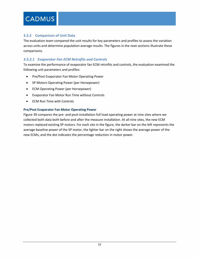
51
3.5.2 Comparison of Unit Data
The evaluation team compared the unit results for key parameters and profiles to assess the variation
across units and determine population average results. The figures in the next sections illustrate these
comparisons.
3.5.2.1 Evaporator Fan ECM Retrofits and Controls
To examine the performance of evaporator fan ECM retrofits and controls, the evaluation examined the
following unit parameters and profiles:
Pre/Post Evaporator Fan Motor Operating Power
SP Motors Operating Power (per Horsepower)
ECM Operating Power (per Horsepower)
Evaporator Fan Motor Run Time without Controls
ECM Run Time with Controls
Pre/Post Evaporator Fan Motor Operating Power
Figure 39 compares the pre- and post-installation full load operating power at nine sites where we
collected both data both before and after the measure installation. At all nine sites, the new ECM
motors replaced existing SP motors. For each site in the figure, the darker bar on the left represents the
average baseline power of the SP motor, the lighter bar on the right shows the average power of the
new ECMs, and the dot indicates the percentage reduction in motor power.
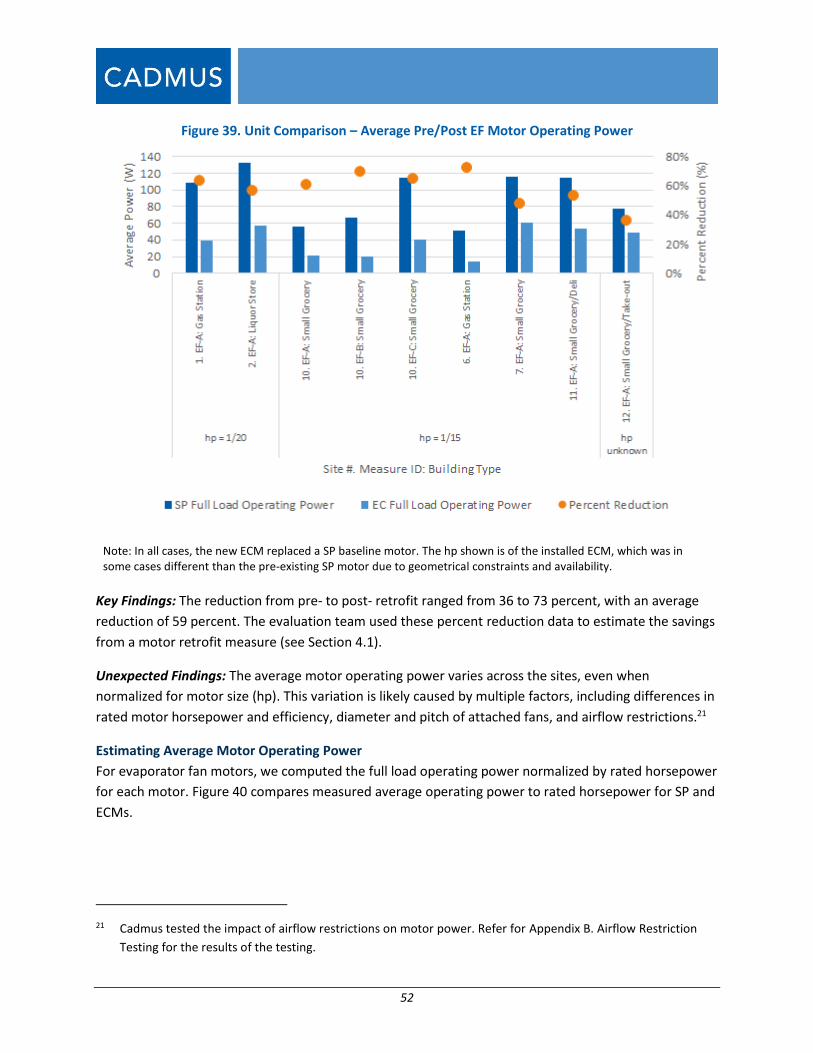
52
Figure 39. Unit Comparison – Average Pre/Post EF Motor Operating Power
Note: In all cases, the new ECM replaced a SP baseline motor. The hp shown is of the installed ECM, which was in some cases different than the pre-existing SP motor due to geometrical constraints and availability.
Key Findings: The reduction from pre- to post- retrofit ranged from 36 to 73 percent, with an average
reduction of 59 percent. The evaluation team used these percent reduction data to estimate the savings
from a motor retrofit measure (see Section 4.1).
Unexpected Findings: The average motor operating power varies across the sites, even when
normalized for motor size (hp). This variation is likely caused by multiple factors, including differences in
rated motor horsepower and efficiency, diameter and pitch of attached fans, and airflow restrictions.21
Estimating Average Motor Operating Power
For evaporator fan motors, we computed the full load operating power normalized by rated horsepower
for each motor. Figure 40 compares measured average operating power to rated horsepower for SP and
ECMs.
21 Cadmus tested the impact of airflow restrictions on motor power. Refer for Appendix B. Airflow Restriction
Testing for the results of the testing.
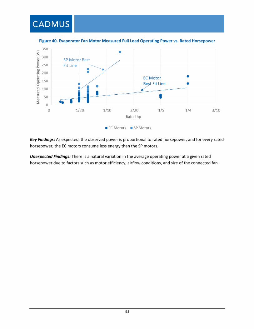
53
Figure 40. Evaporator Fan Motor Measured Full Load Operating Power vs. Rated Horsepower
Key Findings: As expected, the observed power is proportional to rated horsepower, and for every rated
horsepower, the EC motors consume less energy than the SP motors.
Unexpected Findings: There is a natural variation in the average operating power at a given rated
horsepower due to factors such as motor efficiency, airflow conditions, and size of the connected fan.
54
SP Motor Operating Power
Figure 41 compares the full load operating power (normalized by horsepower) for 18 SP motors. The SP
motors are from the nine pre/post sites and nine pre-only sites.
Figure 41. Unit Comparison – Average Baseline EF Motor Operating Power (W/hp)*
Note: In all cases, the baseline motor was SP. *The site numbers beginning with an “S” are from secondary data sources.
Key Findings: The SP motor full load operating power ranged from 1,150 to 3,350 Watts per
horsepower, with an average of 2,088 Watts per horsepower. This is the full load power used to
calculate savings for controls installed on a SP motor.
Unexpected Findings: The variation in SP motor operating power per horsepower is greater than
expected. This is due to a number of factors including the range in efficiencies of motors metered,
diameter and pitch of attached fans, and airflow restrictions.21
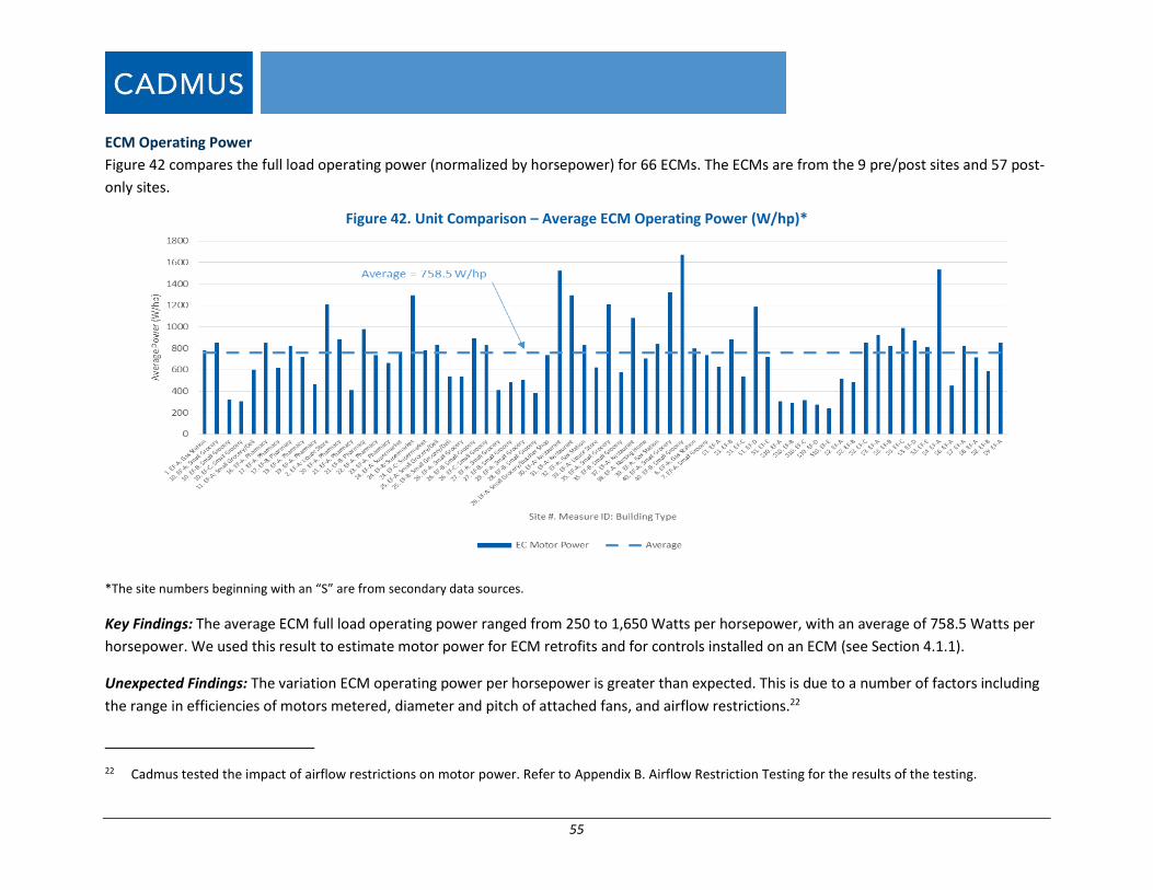
55
ECM Operating Power
Figure 42 compares the full load operating power (normalized by horsepower) for 66 ECMs. The ECMs are from the 9 pre/post sites and 57 post-
only sites.
Figure 42. Unit Comparison – Average ECM Operating Power (W/hp)*
*The site numbers beginning with an “S” are from secondary data sources.
Key Findings: The average ECM full load operating power ranged from 250 to 1,650 Watts per horsepower, with an average of 758.5 Watts per
horsepower. We used this result to estimate motor power for ECM retrofits and for controls installed on an ECM (see Section 4.1.1).
Unexpected Findings: The variation ECM operating power per horsepower is greater than expected. This is due to a number of factors including
the range in efficiencies of motors metered, diameter and pitch of attached fans, and airflow restrictions.22
22 Cadmus tested the impact of airflow restrictions on motor power. Refer to Appendix B. Airflow Restriction Testing for the results of the testing.
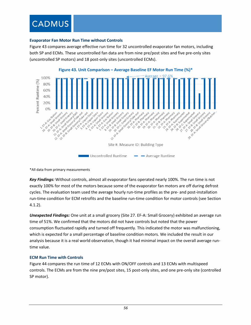
56
Evaporator Fan Motor Run Time without Controls
Figure 43 compares average effective run time for 32 uncontrolled evaporator fan motors, including
both SP and ECMs. These uncontrolled fan data are from nine pre/post sites and five pre-only sites
(uncontrolled SP motors) and 18 post-only sites (uncontrolled ECMs).
Figure 43. Unit Comparison – Average Baseline EF Motor Run Time (%)*
*All data from primary measurements
Key Findings: Without controls, almost all evaporator fans operated nearly 100%. The run time is not
exactly 100% for most of the motors because some of the evaporator fan motors are off during defrost
cycles. The evaluation team used the average hourly run-time profiles as the pre- and post-installation
run-time condition for ECM retrofits and the baseline run-time condition for motor controls (see Section
4.1.2).
Unexpected Findings: One unit at a small grocery (Site 27. EF-A: Small Grocery) exhibited an average run
time of 51%. We confirmed that the motors did not have controls but noted that the power
consumption fluctuated rapidly and turned off frequently. This indicated the motor was malfunctioning,
which is expected for a small percentage of baseline condition motors. We included the result in our
analysis because it is a real world observation, though it had minimal impact on the overall average run-
time value.
ECM Run Time with Controls
Figure 44 compares the run time of 12 ECMs with ON/OFF controls and 13 ECMs with multispeed
controls. The ECMs are from the nine pre/post sites, 15 post-only sites, and one pre-only site (controlled
SP motor).
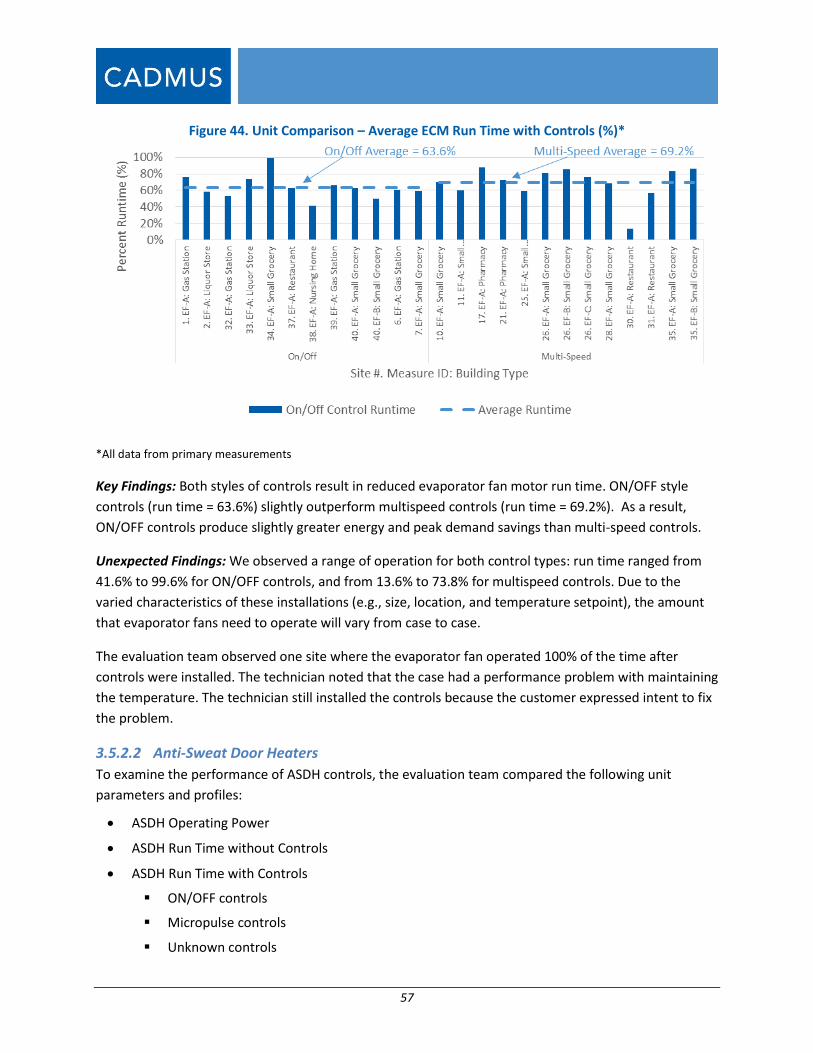
57
Figure 44. Unit Comparison – Average ECM Run Time with Controls (%)*
*All data from primary measurements
Key Findings: Both styles of controls result in reduced evaporator fan motor run time. ON/OFF style
controls (run time = 63.6%) slightly outperform multispeed controls (run time = 69.2%). As a result,
ON/OFF controls produce slightly greater energy and peak demand savings than multi-speed controls.
Unexpected Findings: We observed a range of operation for both control types: run time ranged from
41.6% to 99.6% for ON/OFF controls, and from 13.6% to 73.8% for multispeed controls. Due to the
varied characteristics of these installations (e.g., size, location, and temperature setpoint), the amount
that evaporator fans need to operate will vary from case to case.
The evaluation team observed one site where the evaporator fan operated 100% of the time after
controls were installed. The technician noted that the case had a performance problem with maintaining
the temperature. The technician still installed the controls because the customer expressed intent to fix
the problem.
3.5.2.2 Anti-Sweat Door Heaters
To examine the performance of ASDH controls, the evaluation team compared the following unit
parameters and profiles:
ASDH Operating Power
ASDH Run Time without Controls
ASDH Run Time with Controls
ON/OFF controls
Micropulse controls
Unknown controls
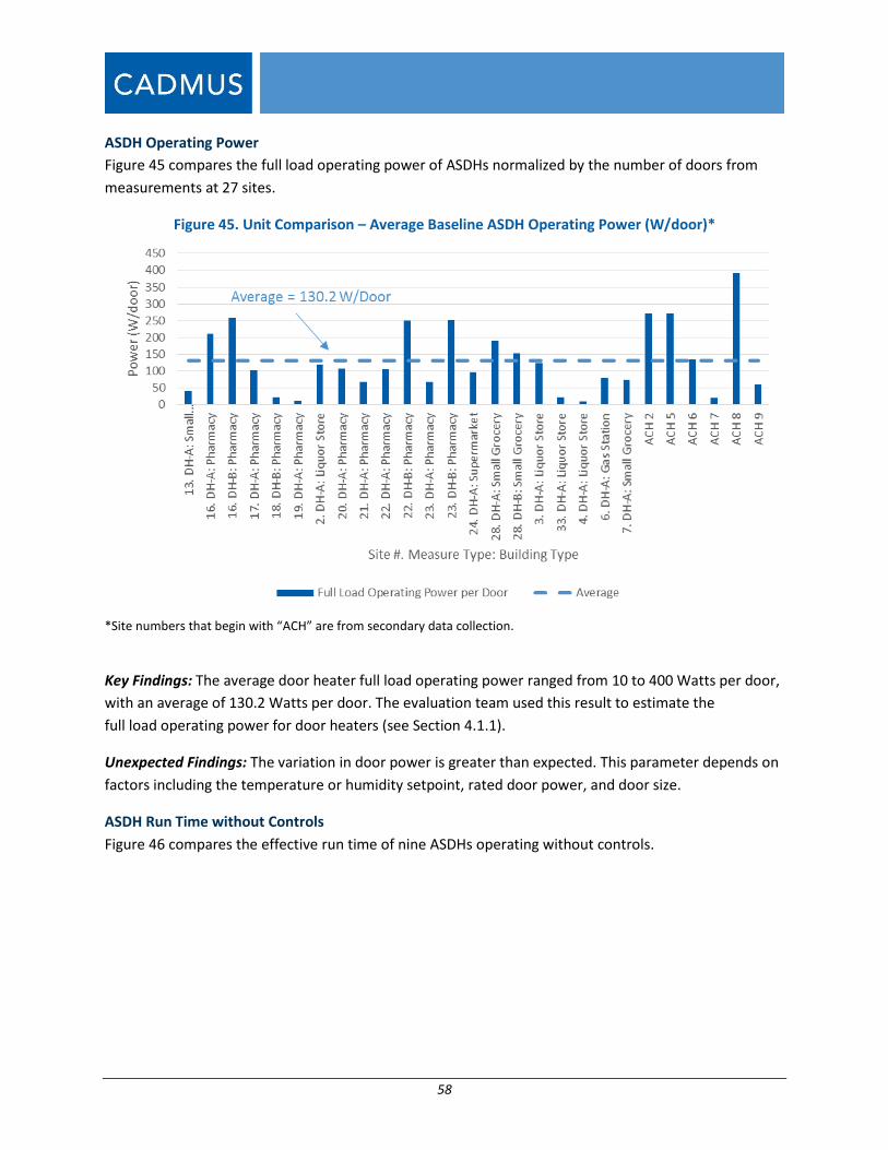
58
ASDH Operating Power
Figure 45 compares the full load operating power of ASDHs normalized by the number of doors from
measurements at 27 sites.
Figure 45. Unit Comparison – Average Baseline ASDH Operating Power (W/door)*
*Site numbers that begin with “ACH” are from secondary data collection.
Key Findings: The average door heater full load operating power ranged from 10 to 400 Watts per door,
with an average of 130.2 Watts per door. The evaluation team used this result to estimate the
full load operating power for door heaters (see Section 4.1.1).
Unexpected Findings: The variation in door power is greater than expected. This parameter depends on
factors including the temperature or humidity setpoint, rated door power, and door size.
ASDH Run Time without Controls
Figure 46 compares the effective run time of nine ASDHs operating without controls.
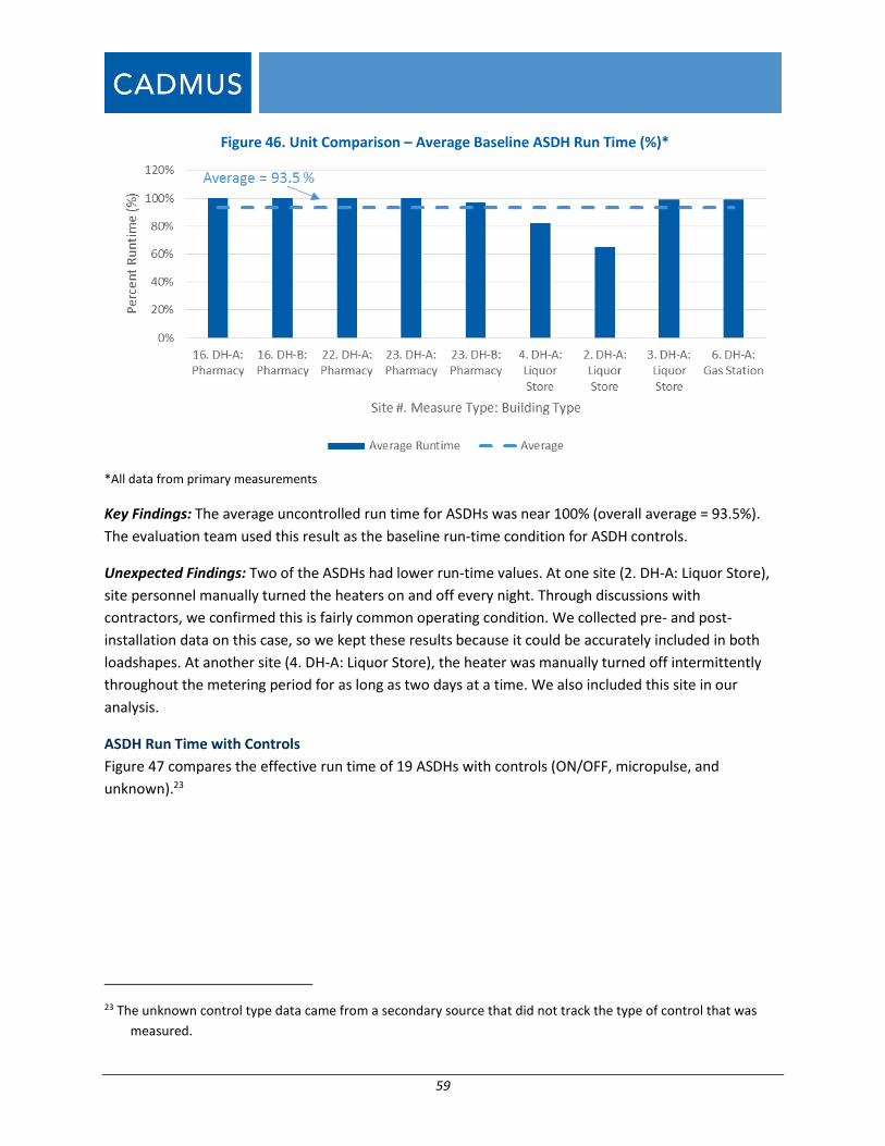
59
Figure 46. Unit Comparison – Average Baseline ASDH Run Time (%)*
*All data from primary measurements
Key Findings: The average uncontrolled run time for ASDHs was near 100% (overall average = 93.5%).
The evaluation team used this result as the baseline run-time condition for ASDH controls.
Unexpected Findings: Two of the ASDHs had lower run-time values. At one site (2. DH-A: Liquor Store),
site personnel manually turned the heaters on and off every night. Through discussions with
contractors, we confirmed this is fairly common operating condition. We collected pre- and post-
installation data on this case, so we kept these results because it could be accurately included in both
loadshapes. At another site (4. DH-A: Liquor Store), the heater was manually turned off intermittently
throughout the metering period for as long as two days at a time. We also included this site in our
analysis.
ASDH Run Time with Controls
Figure 47 compares the effective run time of 19 ASDHs with controls (ON/OFF, micropulse, and
unknown).23
23 The unknown control type data came from a secondary source that did not track the type of control that was
measured.
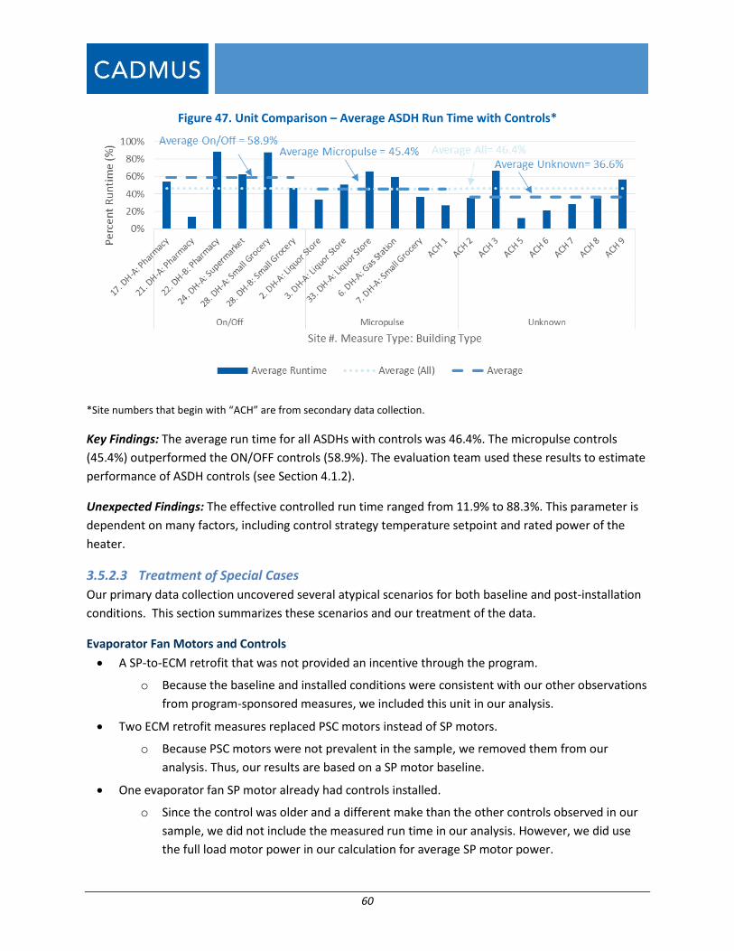
60
Figure 47. Unit Comparison – Average ASDH Run Time with Controls*
*Site numbers that begin with “ACH” are from secondary data collection.
Key Findings: The average run time for all ASDHs with controls was 46.4%. The micropulse controls
(45.4%) outperformed the ON/OFF controls (58.9%). The evaluation team used these results to estimate
performance of ASDH controls (see Section 4.1.2).
Unexpected Findings: The effective controlled run time ranged from 11.9% to 88.3%. This parameter is
dependent on many factors, including control strategy temperature setpoint and rated power of the
heater.
3.5.2.3 Treatment of Special Cases
Our primary data collection uncovered several atypical scenarios for both baseline and post-installation
conditions. This section summarizes these scenarios and our treatment of the data.
Evaporator Fan Motors and Controls
A SP-to-ECM retrofit that was not provided an incentive through the program.
o Because the baseline and installed conditions were consistent with our other observations
from program-sponsored measures, we included this unit in our analysis.
Two ECM retrofit measures replaced PSC motors instead of SP motors.
o Because PSC motors were not prevalent in the sample, we removed them from our
analysis. Thus, our results are based on a SP motor baseline.
One evaporator fan SP motor already had controls installed.
o Since the control was older and a different make than the other controls observed in our
sample, we did not include the measured run time in our analysis. However, we did use
the full load motor power in our calculation for average SP motor power.
61
Controls installed on a SP motor (rather than an ECM) as part of the program.
o We included the run-time profile from this controller in our analysis because (1) the
control type matched other controllers observed in our sample, and (2) contractors
confirmed this was not unusual.
Two evaporator fan controls units were disconnected, resulting in no savings from controls.
o Because contractors confirmed that such removal is not unusual, we included these cases
in our analysis.
At one site, a planned controls installation was cancelled after the implementer advised against
installing controls.
o We used this unit as a baseline condition only to estimate full load operating power and
motor run time without controls.
ASDH Controls
One ASDH unit was not connected (i.e., consumed no power) in the baseline condition. The
implementer re-connected the unit after installing new controls.
o We used only the post-installation data from this site to estimate run time with controls.
At one site, the store manager manually turned off the ASDHs each night.
o We included both the pre- and post-installation condition in our analysis because we
could capture data about the behavior of pre- and post-control installation and because
we confirmed with contractors that it was not unusual.
Three ASDH units exhibited zero savings.
o We were unable to determine what caused these controls to be ineffective but speculated
there could be an issue with the control model, a faulty installation, or user error. Since
we could not determine the cause and because the addition of these three sites would
drastically affect the results due to the small sample size, we excluded these units from
our analysis.
3.5.3 Refrigeration Interactive Effects
As noted in Step 5 (Refrigeration Interactive Effects) and Step 6 (Total Savings Loadshapes)—described
at the beginning of this section, Data Analysis, Figure 25—the total savings from the refrigeration
retrofit measures includes savings resulting from the reduced heat that must be rejected by the
refrigeration equipment. For example, for an ECM retrofit inside a refrigerated space, total savings
includes both the direct power reduction of the more efficient fan motor and the reduced load due to
less waste heat produced by the motors.
The evaluation team developed an Excel-based calculator to estimate these refrigeration interactive
effects for each hour of the year, based on the hourly equipment savings loadshape and ambient
weather data. Figure 48 shows our process for calculating the additional savings from the reduced
refrigeration load.
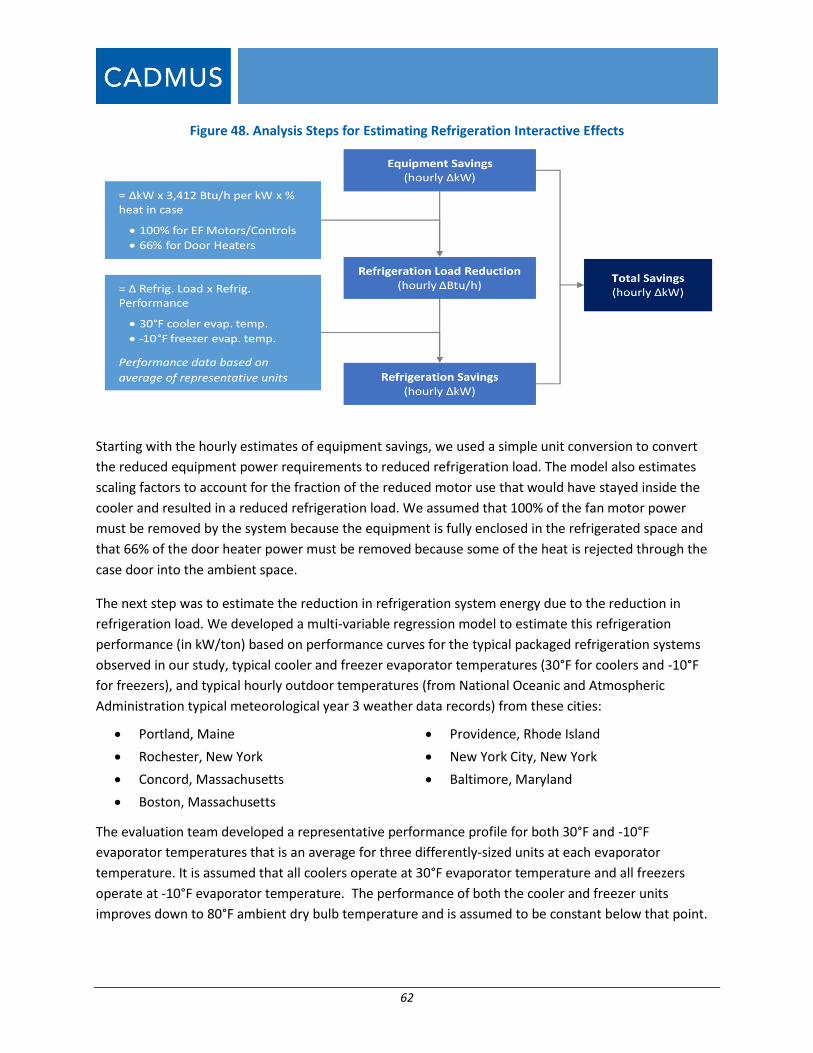
62
Figure 48. Analysis Steps for Estimating Refrigeration Interactive Effects
Starting with the hourly estimates of equipment savings, we used a simple unit conversion to convert
the reduced equipment power requirements to reduced refrigeration load. The model also estimates
scaling factors to account for the fraction of the reduced motor use that would have stayed inside the
cooler and resulted in a reduced refrigeration load. We assumed that 100% of the fan motor power
must be removed by the system because the equipment is fully enclosed in the refrigerated space and
that 66% of the door heater power must be removed because some of the heat is rejected through the
case door into the ambient space.
The next step was to estimate the reduction in refrigeration system energy due to the reduction in
refrigeration load. We developed a multi-variable regression model to estimate this refrigeration
performance (in kW/ton) based on performance curves for the typical packaged refrigeration systems
observed in our study, typical cooler and freezer evaporator temperatures (30°F for coolers and -10°F
for freezers), and typical hourly outdoor temperatures (from National Oceanic and Atmospheric
Administration typical meteorological year 3 weather data records) from these cities:
Portland, Maine
Rochester, New York
Concord, Massachusetts
Boston, Massachusetts
Providence, Rhode Island
New York City, New York
Baltimore, Maryland
The evaluation team developed a representative performance profile for both 30°F and -10°F
evaporator temperatures that is an average for three differently-sized units at each evaporator
temperature. It is assumed that all coolers operate at 30°F evaporator temperature and all freezers
operate at -10°F evaporator temperature. The performance of both the cooler and freezer units
improves down to 80°F ambient dry bulb temperature and is assumed to be constant below that point.
63
The profiles are then used to lookup the performance of either a freezer or cooler unit (kW/ton) at
varying ambient dry bub temperatures.
We assumed the load reduction to be constant for every hour in a typical year and calculated
refrigeration savings using the following equation:
Savings (kW) = Load reduction (kW) × 3,412 BTU/kW ÷ 12,000 BTU/ton × Performance (kW/ton)
Finally, we calculated the total savings by adding refrigeration savings to equipment savings for each
hour of the year. We examined the impacts of these savings by calculating the ratio of total savings to
equipment savings. We refer to this ratio as the bonus factor because it represents the additional or
bonus savings achieved at the refrigeration system when multiplied by the equipment savings. We
found that the savings calculated for each city differed by less than 1%, and therefore determined it is
best to use average values to represent all seven weather regions.
64
4 Results
This study combined primary and secondary data to examine key equipment performance parameters
and develop savings loadshapes for ECM retrofits, evaporator fan motor controls, and ASDH controls. In
this section, we describe the aggregation of the unit-level results to estimate population average
parameters and savings for each measure.
4.1 Population Average Parameters For each result, we compare the average parameters estimated in this study to existing parameters used
in TRMs across the Northeast and Mid-Atlantic, including TRMs in Connecticut, Maine, Massachusetts,
New York, and Vermont.24 We recommend the PAs adopt the population average estimates from this
study as TRM estimates. Based on our review of PA tracking data, our estimates are representative of
the case types (coolers vs. freezers and walk-ins vs. reach-ins) in which measures are installed. We
recommend PAs continue to track these differentiators and recommend additional evaluation research
to grow the metered data sample and develop case-specific results.
4.1.1 Full Load Operating Power for Evaporator Fan Motors
Table 28 shows the average operating power, in units of Watts per horsepower, for evaporator fan
motors and the average percentage change in power observed for ECM retrofit measures. The
population average values are straight averages of the sampled units.
Table 28. Average Parameters – Full Load Operating Power for EF Motors
Parameter Description Source Meter Sample
(# Circuits) Value**
(𝑊𝑆𝑃 − 𝑊𝐸𝐶𝑀
𝑊𝐸𝐶𝑀
) × 100 Percentage change in power
relative to post wattage
Pre/post metering
only*
9 primary
0 secondary 157%
(𝑊
ℎ𝑝)
𝐸𝐶𝑀
ECM power normalized by
horsepower (see Figure 42)
All ECM
measurements
42 primary
24 secondary 758 W/hp
(𝑊
ℎ𝑝)
𝑆𝑃
SP motor power normalized
by horsepower (see Figure
45)
All SP motor
measurements
13 primary
5 secondary 2,088 W/hp
* We calculated this parameter using only data from units where we collected both pre and post measurements.
**Values calculated as straight averages of available primary and secondary data.
Program Administrators can use these Watts per horsepower relationships to estimate motor operating
power given rated horsepower data for the existing or installed motors. If the PA does not have the
rated horsepower information, it should use 1/15 hp based on the size of motor most installed, of the
256 motors observed in this study (see Figure 55).
24 Note that others TRMs – NEEP Mid-Atlantic, etc. do not have this measure listed in the TRM.
65
TRM Comparison
Table 29 compares the average ECM operating power to existing TRM values.
Table 29. TRM Comparison – ECM Operating Power (W/motor)
*Based on measurement of 34 reach-ins and 8 walk-ins. Note: Only the VT TRM provides W/motor values. Other TRMs direct PAs to estimate motor power based on rated Volts, Amps, PF, and other values.
The average NEEP CRL values (based on measurements of 34 reach-ins and 8 walk-ins and an ECM
horsepower of 1/15) is higher than the VT TRM value for ECMs installed in walk-in spaces and much
higher than the VT TRM value for reach-in cases. For PAs not tracking case type (walk-in vs. reach-in) or
motor size we recommend using the NEEP CRL value.
Table 30 compares the average baseline motor power to existing TRM values.
Table 30. TRM Comparison – Baseline Motor Operating Power (W/motor)
*Based on nine measurements at pre/post sites only **Based on measurements at 18 pre-only and pre/post sites ***All measurements on walk-in cases
The average NEEP CRL value is based on SP motors only and assumes a motor size of 1/15 hp. The value
is similar to TRM estimates with two exceptions: the NEEP CRL value is much higher than the VT value
for SP motors in reach-in cases and the value for PSC motors. We recommend PAs update their TRMs
with the W/motor parameter for SP motors in walk-ins that was calculated using both the pre/post and
pre-only sites only (139 W/motor).
Table 31 compares the average motor load reduction factor to existing TRM values. We calculated this
value as the average percent reduction in operating power from pre- (SP motor) to post-retrofit (ECM)
condition of the nine instances where we collected pre- and post-retrofit measurements on the same
exact cases in the same locations.
66
Table 31. TRM Comparison – Load Reduction Factor for ECM Retrofits (%)
*Based on pre- and post-installation measurement of 6 walk-ins and 3 reach-ins
The average NEEP CRL value is based on SP motors only and within the range of TRM estimates for
replacing SP motors with ECMs.25 As expected, the NEEP CRL value is higher than TRM estimates for
replacing PSC motors with ECMs (since PSC motors are more efficient than SP motors). For PAs who do
no tracking case type (walk-in vs. reach-in), we recommend using the NEEP CRL value based on SP
motors only.
4.1.2 Full Load Operating Power for ASDH
Table 32 shows the average operating power, in units of Watts per door, for anti-sweat door heaters.
The population average values are straight averages of the sampled units.
Table 32. Average Parameters – Full Load Operating Power for ASDH
Parameter Description Source Meter Sample
(# Circuits) Value
(𝑊
𝑑𝑜𝑜𝑟)
𝐴𝑆𝐷𝐻 Operating power per door
All door heater
measurements
21 primary
6 secondary
130
W/door
Program administrators can use this average Watts per door value to estimate the full load operating
power for ASDH units. The average number of doors we metered on each circuit was eight. If the PA
does not have information about the number of connected doors per controller or circuit, this is the
number that should be used, i.e., the default savings per controller should be 1,040 W (= 130𝑊
𝑑𝑜𝑜𝑟 ×
8 𝑑𝑜𝑜𝑟𝑠).
TRM Comparison
Table 33 compares the average ASDH power per door to existing TRM values.
25 We observed very few PSC motors in the field so we removed them from our baseline condition.
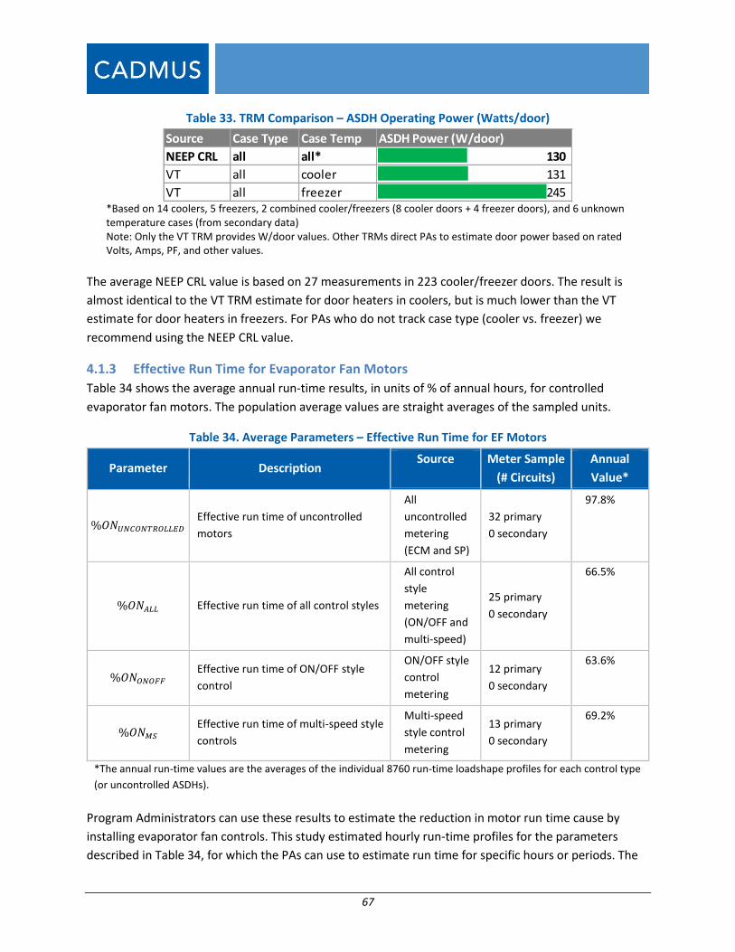
67
Table 33. TRM Comparison – ASDH Operating Power (Watts/door)
*Based on 14 coolers, 5 freezers, 2 combined cooler/freezers (8 cooler doors + 4 freezer doors), and 6 unknown temperature cases (from secondary data) Note: Only the VT TRM provides W/door values. Other TRMs direct PAs to estimate door power based on rated Volts, Amps, PF, and other values.
The average NEEP CRL value is based on 27 measurements in 223 cooler/freezer doors. The result is
almost identical to the VT TRM estimate for door heaters in coolers, but is much lower than the VT
estimate for door heaters in freezers. For PAs who do not track case type (cooler vs. freezer) we
recommend using the NEEP CRL value.
4.1.3 Effective Run Time for Evaporator Fan Motors
Table 34 shows the average annual run-time results, in units of % of annual hours, for controlled
evaporator fan motors. The population average values are straight averages of the sampled units.
Table 34. Average Parameters – Effective Run Time for EF Motors
Parameter Description Source Meter Sample
(# Circuits)
Annual
Value*
%𝑂𝑁𝑈𝑁𝐶𝑂𝑁𝑇𝑅𝑂𝐿𝐿𝐸𝐷 Effective run time of uncontrolled
motors
All
uncontrolled
metering
(ECM and SP)
32 primary
0 secondary
97.8%
%𝑂𝑁𝐴𝐿𝐿 Effective run time of all control styles
All control
style
metering
(ON/OFF and
multi-speed)
25 primary
0 secondary
66.5%
%𝑂𝑁𝑂𝑁𝑂𝐹𝐹 Effective run time of ON/OFF style
control
ON/OFF style
control
metering
12 primary
0 secondary
63.6%
%𝑂𝑁𝑀𝑆 Effective run time of multi-speed style
controls
Multi-speed
style control
metering
13 primary
0 secondary
69.2%
*The annual run-time values are the averages of the individual 8760 run-time loadshape profiles for each control type
(or uncontrolled ASDHs).
Program Administrators can use these results to estimate the reduction in motor run time cause by
installing evaporator fan controls. This study estimated hourly run-time profiles for the parameters
described in Table 34, for which the PAs can use to estimate run time for specific hours or periods. The
Source Case Type Case Temp ASDH Power (W/door)
NEEP CRL all all* 130
VT all cooler 131
VT all freezer 245
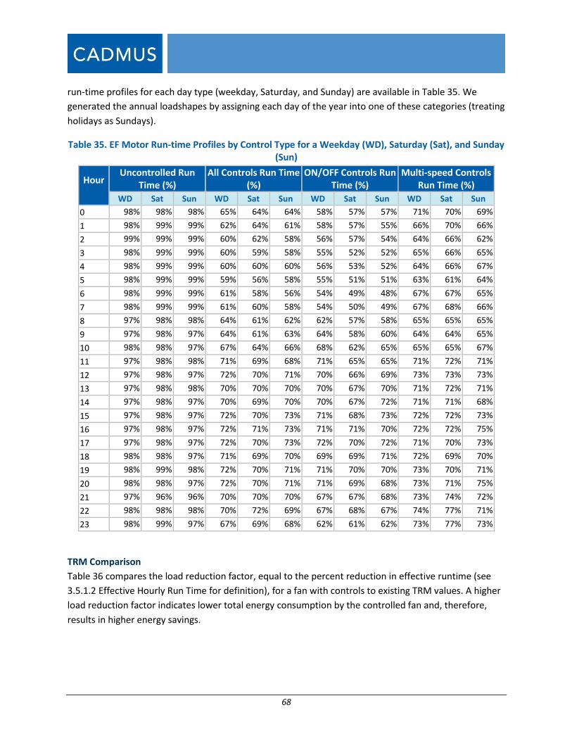
68
run-time profiles for each day type (weekday, Saturday, and Sunday) are available in Table 35. We
generated the annual loadshapes by assigning each day of the year into one of these categories (treating
holidays as Sundays).
Table 35. EF Motor Run-time Profiles by Control Type for a Weekday (WD), Saturday (Sat), and Sunday (Sun)
Hour Uncontrolled Run
Time (%) All Controls Run Time
(%) ON/OFF Controls Run
Time (%) Multi-speed Controls
Run Time (%)
WD Sat Sun WD Sat Sun WD Sat Sun WD Sat Sun
0 98% 98% 98% 65% 64% 64% 58% 57% 57% 71% 70% 69%
1 98% 99% 99% 62% 64% 61% 58% 57% 55% 66% 70% 66%
2 99% 99% 99% 60% 62% 58% 56% 57% 54% 64% 66% 62%
3 98% 99% 99% 60% 59% 58% 55% 52% 52% 65% 66% 65%
4 98% 99% 99% 60% 60% 60% 56% 53% 52% 64% 66% 67%
5 98% 99% 99% 59% 56% 58% 55% 51% 51% 63% 61% 64%
6 98% 99% 99% 61% 58% 56% 54% 49% 48% 67% 67% 65%
7 98% 99% 99% 61% 60% 58% 54% 50% 49% 67% 68% 66%
8 97% 98% 98% 64% 61% 62% 62% 57% 58% 65% 65% 65%
9 97% 98% 97% 64% 61% 63% 64% 58% 60% 64% 64% 65%
10 98% 98% 97% 67% 64% 66% 68% 62% 65% 65% 65% 67%
11 97% 98% 98% 71% 69% 68% 71% 65% 65% 71% 72% 71%
12 97% 98% 97% 72% 70% 71% 70% 66% 69% 73% 73% 73%
13 97% 98% 98% 70% 70% 70% 70% 67% 70% 71% 72% 71%
14 97% 98% 97% 70% 69% 70% 70% 67% 72% 71% 71% 68%
15 97% 98% 97% 72% 70% 73% 71% 68% 73% 72% 72% 73%
16 97% 98% 97% 72% 71% 73% 71% 71% 70% 72% 72% 75%
17 97% 98% 97% 72% 70% 73% 72% 70% 72% 71% 70% 73%
18 98% 98% 97% 71% 69% 70% 69% 69% 71% 72% 69% 70%
19 98% 99% 98% 72% 70% 71% 71% 70% 70% 73% 70% 71%
20 98% 98% 97% 72% 70% 71% 71% 69% 68% 73% 71% 75%
21 97% 96% 96% 70% 70% 70% 67% 67% 68% 73% 74% 72%
22 98% 98% 98% 70% 72% 69% 67% 68% 67% 74% 77% 71%
23 98% 99% 97% 67% 69% 68% 62% 61% 62% 73% 77% 73%
TRM Comparison
Table 36 compares the load reduction factor, equal to the percent reduction in effective runtime (see
3.5.1.2 Effective Hourly Run Time for definition), for a fan with controls to existing TRM values. A higher
load reduction factor indicates lower total energy consumption by the controlled fan and, therefore,
results in higher energy savings.
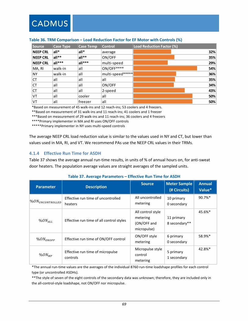
69
Table 36. TRM Comparison – Load Reduction Factor for EF Motor with Controls (%)
*Based on measurement of 45 walk-ins and 12 reach-ins; 53 coolers and 4 freezers. **Based on measurement of 31 walk-ins and 11 reach-ins; 41 coolers and 1 freezer ***Based on measurement of 29 walk-ins and 11 reach-ins; 36 coolers and 4 freezers ****Primary implementer in MA and RI uses ON/OFF controls *****Primary implementer in NY uses multi-speed controls
The average NEEP CRL load reduction value is similar to the values used in NY and CT, but lower than
values used in MA, RI, and VT. We recommend PAs use the NEEP CRL values in their TRMs.
4.1.4 Effective Run Time for ASDH
Table 37 shows the average annual run-time results, in units of % of annual hours on, for anti-sweat
door heaters. The population average values are straight averages of the sampled units.
Table 37. Average Parameters – Effective Run Time for ASDH
Parameter Description Source Meter Sample
(# Circuits)
Annual
Value*
%𝑂𝑁𝑈𝑁𝐶𝑂𝑁𝑇𝑅𝑂𝐿𝐿𝐸𝐷 Effective run time of uncontrolled
heaters
All uncontrolled
metering 10 primary
0 secondary
90.7%*
%𝑂𝑁𝐴𝐿𝐿 Effective run time of all control styles
All control style
metering
(ON/OFF and
micropulse)
11 primary
8 secondary**
45.6%*
%𝑂𝑁𝑂𝑁𝑂𝐹𝐹 Effective run time of ON/OFF control ON/OFF style
metering
6 primary
0 secondary
58.9%*
%𝑂𝑁𝑀𝑃 Effective run time of micropulse
controls
Micropulse style
control
metering
5 primary
1 secondary
42.8%*
*The annual run-time values are the averages of the individual 8760 run-time loadshape profiles for each control
type (or uncontrolled ASDHs). **The style of seven of the eight controls of the secondary data was unknown; therefore, they are included only in
the all-control-style loadshape, not ON/OFF nor micropulse.
Source Case Type Case Temp Control Load Reduction Factor (%)
NEEP CRL all* all* average 32%
NEEP CRL all** all** ON/OFF 35%
NEEP CRL all*** all*** multi-speed 29%
MA, RI walk-in all ON/OFF**** 54%
NY walk-in all multi-speed***** 36%
CT all all all 35%
CT all all ON/OFF 34%
CT all all 2-speed 43%
VT all cooler all 50%
VT all freezer all 50%
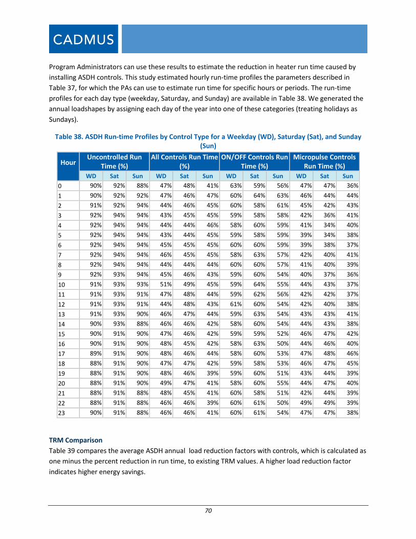
70
Program Administrators can use these results to estimate the reduction in heater run time caused by
installing ASDH controls. This study estimated hourly run-time profiles the parameters described in
Table 37, for which the PAs can use to estimate run time for specific hours or periods. The run-time
profiles for each day type (weekday, Saturday, and Sunday) are available in Table 38. We generated the
annual loadshapes by assigning each day of the year into one of these categories (treating holidays as
Sundays).
Table 38. ASDH Run-time Profiles by Control Type for a Weekday (WD), Saturday (Sat), and Sunday (Sun)
Hour Uncontrolled Run
Time (%) All Controls Run Time
(%) ON/OFF Controls Run
Time (%) Micropulse Controls
Run Time (%)
WD Sat Sun WD Sat Sun WD Sat Sun WD Sat Sun
0 90% 92% 88% 47% 48% 41% 63% 59% 56% 47% 47% 36%
1 90% 92% 92% 47% 46% 47% 60% 64% 63% 46% 44% 44%
2 91% 92% 94% 44% 46% 45% 60% 58% 61% 45% 42% 43%
3 92% 94% 94% 43% 45% 45% 59% 58% 58% 42% 36% 41%
4 92% 94% 94% 44% 44% 46% 58% 60% 59% 41% 34% 40%
5 92% 94% 94% 43% 44% 45% 59% 58% 59% 39% 34% 38%
6 92% 94% 94% 45% 45% 45% 60% 60% 59% 39% 38% 37%
7 92% 94% 94% 46% 45% 45% 58% 63% 57% 42% 40% 41%
8 92% 94% 94% 44% 44% 44% 60% 60% 57% 41% 40% 39%
9 92% 93% 94% 45% 46% 43% 59% 60% 54% 40% 37% 36%
10 91% 93% 93% 51% 49% 45% 59% 64% 55% 44% 43% 37%
11 91% 93% 91% 47% 48% 44% 59% 62% 56% 42% 42% 37%
12 91% 93% 91% 44% 48% 43% 61% 60% 54% 42% 40% 38%
13 91% 93% 90% 46% 47% 44% 59% 63% 54% 43% 43% 41%
14 90% 93% 88% 46% 46% 42% 58% 60% 54% 44% 43% 38%
15 90% 91% 90% 47% 46% 42% 59% 59% 52% 46% 47% 42%
16 90% 91% 90% 48% 45% 42% 58% 63% 50% 44% 46% 40%
17 89% 91% 90% 48% 46% 44% 58% 60% 53% 47% 48% 46%
18 88% 91% 90% 47% 47% 42% 59% 58% 53% 46% 47% 45%
19 88% 91% 90% 48% 46% 39% 59% 60% 51% 43% 44% 39%
20 88% 91% 90% 49% 47% 41% 58% 60% 55% 44% 47% 40%
21 88% 91% 88% 48% 45% 41% 60% 58% 51% 42% 44% 39%
22 88% 91% 88% 46% 46% 39% 60% 61% 50% 49% 49% 39%
23 90% 91% 88% 46% 46% 41% 60% 61% 54% 47% 47% 38%
TRM Comparison
Table 39 compares the average ASDH annual load reduction factors with controls, which is calculated as
one minus the percent reduction in run time, to existing TRM values. A higher load reduction factor
indicates higher energy savings.
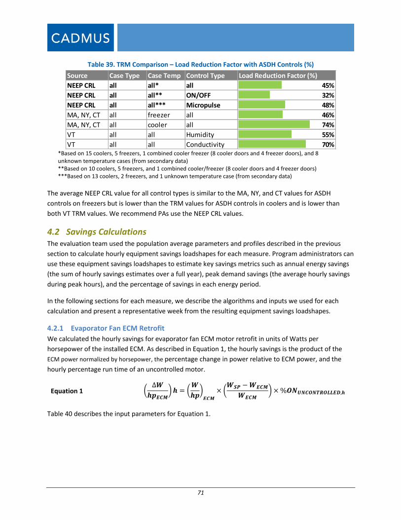
71
Table 39. TRM Comparison – Load Reduction Factor with ASDH Controls (%)
*Based on 15 coolers, 5 freezers, 1 combined cooler freezer (8 cooler doors and 4 freezer doors), and 8 unknown temperature cases (from secondary data) **Based on 10 coolers, 5 freezers, and 1 combined cooler/freezer (8 cooler doors and 4 freezer doors) ***Based on 13 coolers, 2 freezers, and 1 unknown temperature case (from secondary data)
The average NEEP CRL value for all control types is similar to the MA, NY, and CT values for ASDH
controls on freezers but is lower than the TRM values for ASDH controls in coolers and is lower than
both VT TRM values. We recommend PAs use the NEEP CRL values.
4.2 Savings Calculations The evaluation team used the population average parameters and profiles described in the previous
section to calculate hourly equipment savings loadshapes for each measure. Program administrators can
use these equipment savings loadshapes to estimate key savings metrics such as annual energy savings
(the sum of hourly savings estimates over a full year), peak demand savings (the average hourly savings
during peak hours), and the percentage of savings in each energy period.
In the following sections for each measure, we describe the algorithms and inputs we used for each
calculation and present a representative week from the resulting equipment savings loadshapes.
4.2.1 Evaporator Fan ECM Retrofit
We calculated the hourly savings for evaporator fan ECM motor retrofit in units of Watts per
horsepower of the installed ECM. As described in Equation 1, the hourly savings is the product of the
ECM power normalized by horsepower, the percentage change in power relative to ECM power, and the
hourly percentage run time of an uncontrolled motor.
Equation 1 (∆𝑾
𝒉𝒑𝑬𝑪𝑴) 𝒉 = (
𝑾
𝒉𝒑)
𝑬𝑪𝑴
× (𝑾𝑺𝑷 − 𝑾𝑬𝑪𝑴
𝑾𝑬𝑪𝑴) × %𝑶𝑵𝑼𝑵𝑪𝑶𝑵𝑻𝑹𝑶𝑳𝑳𝑬𝑫,𝒉
Table 40 describes the input parameters for Equation 1.
Source Case Type Case Temp Control Type Load Reduction Factor (%)
NEEP CRL all all* all 45%
NEEP CRL all all** ON/OFF 32%
NEEP CRL all all*** Micropulse 48%
MA, NY, CT all freezer all 46%
MA, NY, CT all cooler all 74%
VT all all Humidity 55%
VT all all Conductivity 70%
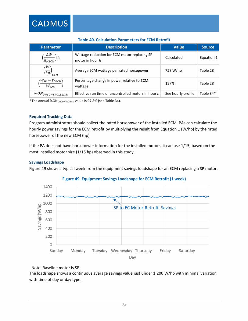
72
Table 40. Calculation Parameters for ECM Retrofit
Parameter Description Value Source
(∆𝑊
ℎ𝑝𝐸𝐶𝑀
) ℎ Wattage reduction for ECM motor replacing SP
motor in hour h Calculated Equation 1
(𝑊
ℎ𝑝)
𝐸𝐶𝑀
Average ECM wattage per rated horsepower 758 W/hp Table 28
(𝑊𝑆𝑃 − 𝑊𝐸𝐶𝑀
𝑊𝐸𝐶𝑀
) Percentage change in power relative to ECM
wattage 157% Table 28
%𝑂𝑁𝑈𝑁𝐶𝑂𝑁𝑇𝑅𝑂𝐿𝐿𝐸𝐷,ℎ Effective run time of uncontrolled motors in hour h See hourly profile Table 34*
*The annual %ONUNCONTROLLED value is 97.8% (see Table 34).
Required Tracking Data
Program administrators should collect the rated horsepower of the installed ECM. PAs can calculate the
hourly power savings for the ECM retrofit by multiplying the result from Equation 1 (W/hp) by the rated
horsepower of the new ECM (hp).
If the PA does not have horsepower information for the installed motors, it can use 1/15, based on the
most installed motor size (1/15 hp) observed in this study.
Savings Loadshape
Figure 49 shows a typical week from the equipment savings loadshape for an ECM replacing a SP motor.
Figure 49. Equipment Savings Loadshape for ECM Retrofit (1 week)
Note: Baseline motor is SP.
The loadshape shows a continuous average savings value just under 1,200 W/hp with minimal variation
with time of day or day type.

73
4.2.2 Evaporator Fan Motor Controls
We calculated the hourly savings for evaporator fan motor controls installed on ECMs or SP motors in
units of Watts per horsepower of the installed motor. As described in Equation 2 and Equation 3, the
hourly savings is the product of the motor wattage normalized by horsepower and the difference in
hourly run time between an uncontrolled and controlled motor.
Equation 2 (EF motor controls on ECM)
(∆𝑾
𝒉𝒑𝑬𝑪𝑴) 𝒉 = (
𝑾
𝒉𝒑)
𝑬𝑪𝑴
× (%𝑶𝑵𝑼𝑵𝑪𝑶𝑵𝑻𝑹𝑶𝑳𝑳𝑬𝑫 − %𝑶𝑵𝑿)𝒉
Equation 3 (EF motor controls on SP motor)
(∆𝑾
𝒉𝒑𝑺𝑷)
𝒉
= (𝑾
𝒉𝒑)
𝑺𝑷
× (%𝑶𝑵𝑼𝑵𝑪𝑶𝑵𝑻𝑹𝑶𝑳𝑳𝑬𝑫 − %𝑶𝑵𝑿)𝒉
Table 40 describes the input parameters for Equation 2 and Equation 3.
Table 41. Calculation Parameters for EF Motor Controls
Parameter Description Value Source
(∆𝑊
ℎ𝑝𝐸𝐶𝑀
)ℎ
Wattage reduction for EF controls on an ECM in hour h Calculated Equation 2
(𝑊
ℎ𝑝)
𝐸𝐶𝑀
Average ECM wattage per rated horsepower 758 W/hp Table 28
(∆𝑊
ℎ𝑝𝑆𝑃
)ℎ
Wattage reduction for EF controls on a SP motor in hour h Calculated Equation 3
(𝑊
ℎ𝑝)
𝑆𝑃
Average SP wattage per rated horsepower 2,088 W/hp Table 28
%𝑂𝑁𝑈𝑁𝐶𝑂𝑁𝑇𝑅𝑂𝐿𝐿𝐸𝐷,ℎ Effective run time of uncontrolled motor in hour h Hourly profile Table 34*
%𝑂𝑁𝑋,ℎ Effective run time of motor with control type X in hour h Hourly profile Table 34*
*The annual %ONUNCONTROLLED value is 97.8% (see Table 34).
Required Tracking Data
Program administrators should collect the rated horsepower of the motor on which the controls are
installed. PAs can calculate the hourly power savings for the EF motor controls by multiplying the result
from Equation 2 (for ECMs) or Equation 3 (for SP motors) (W/hp) by the rated horsepower of the
installed motor (hp).
If the PA does not have horsepower information for the installed motors, it can use 1/15 for ECMs or SP
motors.
Savings Loadshape
Figure 50 shows a representative week from the equipment savings loadshape for evaporator fan motor
controls. The figure shows results for multiple control types installed on SP motors and ECMs.
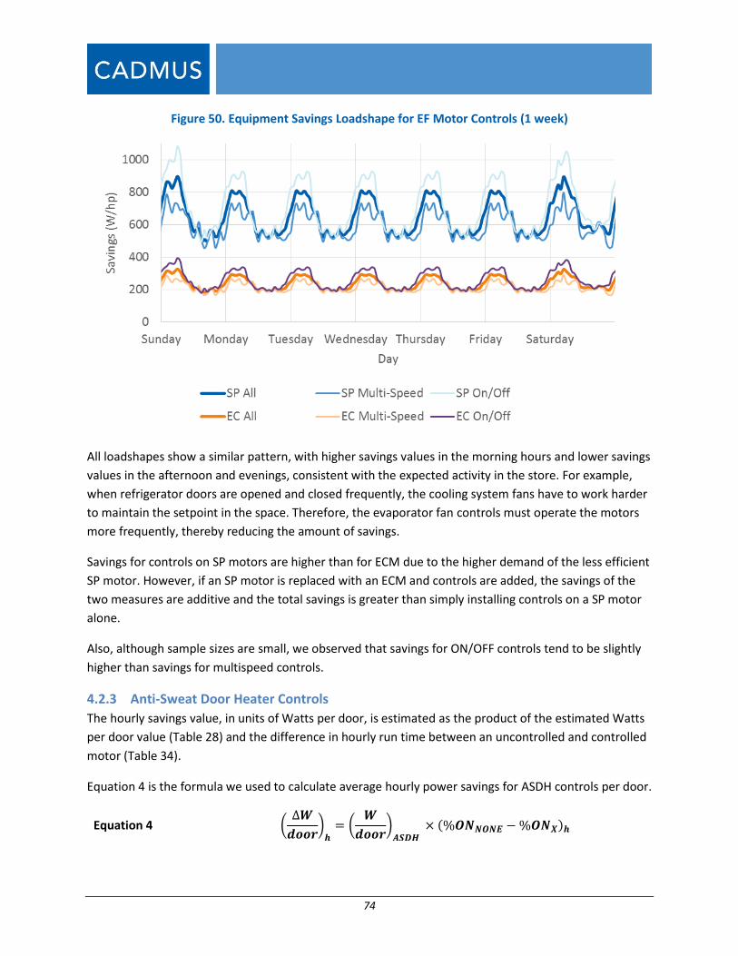
74
Figure 50. Equipment Savings Loadshape for EF Motor Controls (1 week)
All loadshapes show a similar pattern, with higher savings values in the morning hours and lower savings
values in the afternoon and evenings, consistent with the expected activity in the store. For example,
when refrigerator doors are opened and closed frequently, the cooling system fans have to work harder
to maintain the setpoint in the space. Therefore, the evaporator fan controls must operate the motors
more frequently, thereby reducing the amount of savings.
Savings for controls on SP motors are higher than for ECM due to the higher demand of the less efficient
SP motor. However, if an SP motor is replaced with an ECM and controls are added, the savings of the
two measures are additive and the total savings is greater than simply installing controls on a SP motor
alone.
Also, although sample sizes are small, we observed that savings for ON/OFF controls tend to be slightly
higher than savings for multispeed controls.
4.2.3 Anti-Sweat Door Heater Controls
The hourly savings value, in units of Watts per door, is estimated as the product of the estimated Watts
per door value (Table 28) and the difference in hourly run time between an uncontrolled and controlled
motor (Table 34).
Equation 4 is the formula we used to calculate average hourly power savings for ASDH controls per door.
Equation 4 (∆𝑾
𝒅𝒐𝒐𝒓)
𝒉= (
𝑾
𝒅𝒐𝒐𝒓)
𝑨𝑺𝑫𝑯 × (%𝑶𝑵𝑵𝑶𝑵𝑬 − %𝑶𝑵𝑿)𝒉
75
Table 42 describes the input parameters for Equation 4.
Table 42. Calculation Parameters for ASDH Controls
Parameter Description Value Source
(∆𝑊
𝑑𝑜𝑜𝑟)
ℎ
Wattage reduction per connected door for ASDH
controls in hour h Calculated Equation 4
(𝑊
𝑑𝑜𝑜𝑟)
𝐴𝑆𝐷𝐻 Average wattage of ASDH per connected door 130 W/door Table 32
%𝑂𝑁𝑁𝑂𝑁𝐸,ℎ Effective run time of uncontrolled ASDH in hour h Hourly profile Table 37*
%𝑂𝑁𝑋,ℎ Effective run time of ASDH with control type X in hour
h Hourly profile Table 37**
*The annual %ONUNCONTROLLED value is 90.7% (see Table 37).
**The annual %ONX value is 45.6% for all controls, 58.9% for ON/OFF controls, and 42.8% for micropulse controls (see
Table 37).
Required Tracking Data
Program administrators should collect the number of doors connected to the ASDH controller installed.
PAs can calculate the hourly power savings for ASDH controls by multiplying the result from Equation 4
(W/door) by the number of doors connected to the ASDH control or controls.
The average number of doors we metered on each circuit was 8. If the PA does not have information
about the number of connected doors per controller or circuit, this is the number that should be used.
Savings Loadshape
Figure 51 shows a typical week from the equipment savings loadshapes for ASDH controls. The figure
shows multiple control types as well as an average loadshape for all control types.
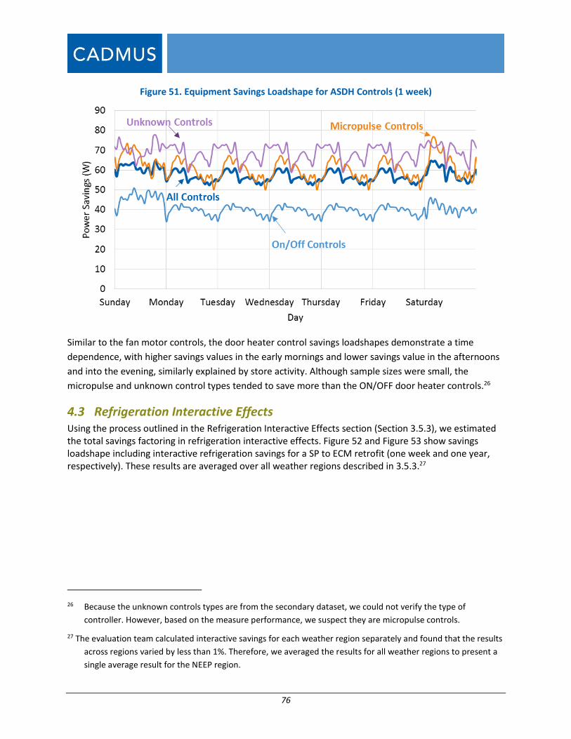
76
Figure 51. Equipment Savings Loadshape for ASDH Controls (1 week)
Similar to the fan motor controls, the door heater control savings loadshapes demonstrate a time
dependence, with higher savings values in the early mornings and lower savings value in the afternoons
and into the evening, similarly explained by store activity. Although sample sizes were small, the
micropulse and unknown control types tended to save more than the ON/OFF door heater controls.26
4.3 Refrigeration Interactive Effects Using the process outlined in the Refrigeration Interactive Effects section (Section 3.5.3), we estimated the total savings factoring in refrigeration interactive effects. Figure 52 and Figure 53 show savings loadshape including interactive refrigeration savings for a SP to ECM retrofit (one week and one year, respectively). These results are averaged over all weather regions described in 3.5.3.27
26 Because the unknown controls types are from the secondary dataset, we could not verify the type of
controller. However, based on the measure performance, we suspect they are micropulse controls.
27 The evaluation team calculated interactive savings for each weather region separately and found that the results
across regions varied by less than 1%. Therefore, we averaged the results for all weather regions to present a
single average result for the NEEP region.
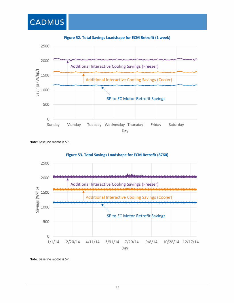
77
Figure 52. Total Savings Loadshape for ECM Retrofit (1 week)
Note: Baseline motor is SP.
Figure 53. Total Savings Loadshape for ECM Retrofit (8760)
Note: Baseline motor is SP.
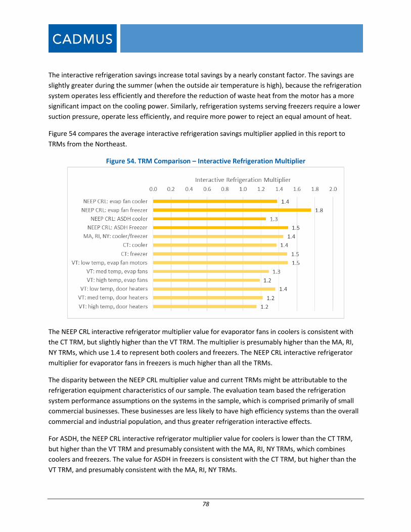
78
The interactive refrigeration savings increase total savings by a nearly constant factor. The savings are
slightly greater during the summer (when the outside air temperature is high), because the refrigeration
system operates less efficiently and therefore the reduction of waste heat from the motor has a more
significant impact on the cooling power. Similarly, refrigeration systems serving freezers require a lower
suction pressure, operate less efficiently, and require more power to reject an equal amount of heat.
Figure 54 compares the average interactive refrigeration savings multiplier applied in this report to
TRMs from the Northeast.
Figure 54. TRM Comparison – Interactive Refrigeration Multiplier
The NEEP CRL interactive refrigerator multiplier value for evaporator fans in coolers is consistent with
the CT TRM, but slightly higher than the VT TRM. The multiplier is presumably higher than the MA, RI,
NY TRMs, which use 1.4 to represent both coolers and freezers. The NEEP CRL interactive refrigerator
multiplier for evaporator fans in freezers is much higher than all the TRMs.
The disparity between the NEEP CRL multiplier value and current TRMs might be attributable to the
refrigeration equipment characteristics of our sample. The evaluation team based the refrigeration
system performance assumptions on the systems in the sample, which is comprised primarily of small
commercial businesses. These businesses are less likely to have high efficiency systems than the overall
commercial and industrial population, and thus greater refrigeration interactive effects.
For ASDH, the NEEP CRL interactive refrigerator multiplier value for coolers is lower than the CT TRM,
but higher than the VT TRM and presumably consistent with the MA, RI, NY TRMs, which combines
coolers and freezers. The value for ASDH in freezers is consistent with the CT TRM, but higher than the
VT TRM, and presumably consistent with the MA, RI, NY TRMs.
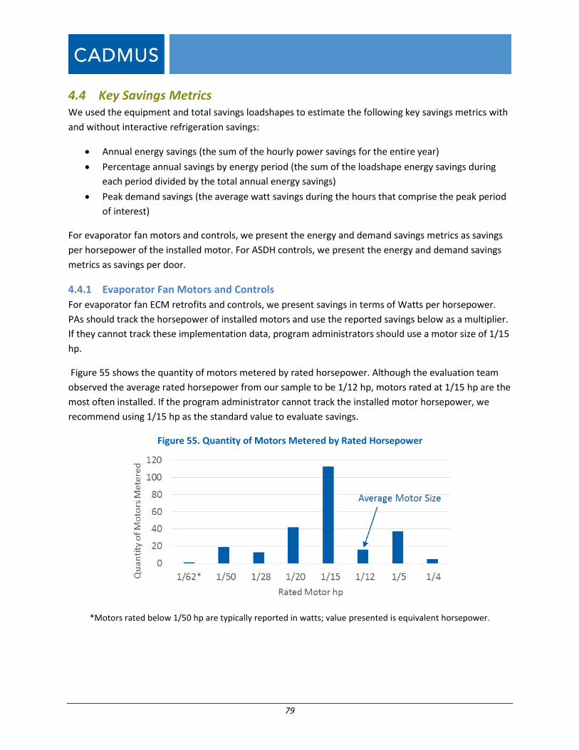
79
4.4 Key Savings Metrics We used the equipment and total savings loadshapes to estimate the following key savings metrics with
and without interactive refrigeration savings:
Annual energy savings (the sum of the hourly power savings for the entire year)
Percentage annual savings by energy period (the sum of the loadshape energy savings during
each period divided by the total annual energy savings)
Peak demand savings (the average watt savings during the hours that comprise the peak period
of interest)
For evaporator fan motors and controls, we present the energy and demand savings metrics as savings
per horsepower of the installed motor. For ASDH controls, we present the energy and demand savings
metrics as savings per door.
4.4.1 Evaporator Fan Motors and Controls
For evaporator fan ECM retrofits and controls, we present savings in terms of Watts per horsepower.
PAs should track the horsepower of installed motors and use the reported savings below as a multiplier.
If they cannot track these implementation data, program administrators should use a motor size of 1/15
hp.
Figure 55 shows the quantity of motors metered by rated horsepower. Although the evaluation team
observed the average rated horsepower from our sample to be 1/12 hp, motors rated at 1/15 hp are the
most often installed. If the program administrator cannot track the installed motor horsepower, we
recommend using 1/15 hp as the standard value to evaluate savings.
Figure 55. Quantity of Motors Metered by Rated Horsepower
*Motors rated below 1/50 hp are typically reported in watts; value presented is equivalent horsepower.
80
4.4.1.1 Annual Energy Savings
Table 43 summarizes the annual energy savings in kWh/hp for all evaporator fan motor measures. We
presented the results in terms of the horsepower of the post-installation measure, i.e., the ECM for a SP
to ECM retrofit or whatever unit the motor controls are installed on.
Table 43. Annual Energy Savings for EF Motors and Controls
Equipment Type
Annual Energy Savings (kWh/hp) Relative Precision (%)
Equipment Only
Equipment and Interactive (Cooler)*
Equipment and Interactive (Freezer)*
90% Confidence
80% Confidence
SP to ECM Retrofit 10,198 14,122 17,944 5% 4%
EF Controls on SP Motor (All) 5,712 7,908 10,048 3% 2%
EF Controls on SP Motor (OnOff) 6,248 8,650 10,991 3% 3%
EF Controls on SP Motor (MS) 5,217 7,224 9,178 5% 4%
EF Controls on ECM (All) 2,074 2,872 3,650 2% 2%
EF Controls on ECM (OnOff) 2,269 3,142 3,992 2% 2%
EF Controls on ECM (MS) 1,895 2,624 3,334 3% 3%
*Interactive savings are averaged over the weather regions shown in section 3.5.3 because the variation among regions was less than 1%.
The savings from adding controls to an SP motor are greater than an ECM; however, the savings for
adding controls to an ECM are incremental to the SP to ECM retrofit if both measures are performed
together. For example, using the average of all control types, the savings for installing controls on an SP
motor are 5,712 kWh/hp, but the savings from replacing the SP motor with an ECM and adding controls
is 10,198 + 2,074 = 12,272 kWh/hp. Thus, replacing a SP motor and adding controls results in
significantly more savings than just adding controls.
Table 44 shows the distribution of annual energy savings from evaporator fan measures in each energy
period.28
28 Summer on peak comprises 7:00 AM to 11:00 PM on non-holiday weekdays in June through September; summer
off peak comprises 11:00 pm – 7:AM on non-holiday weekdays and all hours on weekends and holidays in June
through September; winter on peak comprises 7:00 AM to 11:00 PM on non-holiday weekdays in October
through May; and winter off peak comprises 11:00 PM to 7:00 AM on non-holiday weekdays and all hours on
weekends and holidays in October through May.
81
Table 44. Energy Period Allocations for EF Motors and Controls
Equipment Type
Summer On Peak Summer Off Peak Winter On Peak Winter Off Peak
% RP@ 90%
RP@ 80%
% RP@ 90%
RP@ 80%
% RP@ 90%
RP@ 80%
% RP@ 90%
RP@ 80%
Equipment Only
SP to ECM Retrofit 15% 7% 5% 18% 18% 18% 30% 30% 30% 37% 37% 37%
EF Controls on SP Motor (All) 14% 5% 4% 19% 19% 19% 27% 27% 27% 40% 40% 40%
EF Controls on SP Motor (OnOff) 13% 6% 4% 20% 20% 20% 26% 25% 25% 41% 41% 41%
EF Controls on SP Motor (MS) 15% 8% 6% 19% 19% 19% 28% 28% 28% 39% 39% 39%
EF Controls on ECM (All) 14% 5% 4% 19% 19% 19% 27% 27% 27% 40% 40% 40%
EF Controls on ECM (OnOff) 13% 5% 4% 20% 20% 20% 26% 25% 25% 41% 41% 41%
EF Controls on ECM (MS) 15% 8% 6% 19% 19% 19% 28% 28% 28% 39% 39% 39%
Equipment and Interactive (Cooler)*
SP to ECM Retrofit 15% 7% 5% 18% 18% 18% 30% 30% 30% 37% 37% 37%
EF Controls on SP Motor (All) 14% 5% 4% 19% 19% 19% 27% 27% 27% 40% 40% 40%
EF Controls on SP Motor (OnOff) 13% 6% 4% 20% 20% 20% 25% 25% 25% 41% 41% 41%
EF Controls on SP Motor (MS) 15% 8% 6% 19% 19% 19% 28% 28% 28% 39% 39% 39%
EF Controls on ECM (All) 14% 5% 4% 19% 19% 19% 27% 27% 27% 40% 40% 40%
EF Controls on ECM (OnOff) 13% 5% 4% 20% 20% 20% 25% 25% 25% 41% 41% 41%
EF Controls on ECM (MS) 15% 8% 6% 19% 19% 19% 28% 28% 28% 39% 39% 39%
Equipment and Interactive (Freezer)*
SP to ECM Retrofit 16% 7% 5% 18% 18% 18% 30% 30% 30% 37% 37% 37%
EF Controls on SP Motor (All) 14% 5% 4% 19% 19% 19% 27% 27% 27% 40% 40% 40%
EF Controls on SP Motor (OnOff) 13% 6% 4% 20% 20% 20% 25% 25% 25% 41% 41% 41%
EF Controls on SP Motor (MS) 15% 8% 6% 19% 19% 19% 28% 28% 28% 39% 39% 39%
EF Controls on ECM (All) 14% 5% 4% 19% 19% 19% 27% 27% 27% 40% 40% 40%
EF Controls on ECM (OnOff) 13% 5% 4% 20% 20% 20% 25% 25% 25% 41% 41% 41%
EF Controls on ECM (MS) 15% 8% 6% 19% 19% 19% 28% 28% 28% 39% 39% 39%
*Interactive savings are averaged over the weather regions shown in section 3.5.3 because the variation among regions was less than 1%.
4.4.1.2 Peak Demand Savings
Table 45 (ISO-NE summer peak), Table 46 (ISO-NE winter peak), and Table 47 (PJM summer peak) show
peak demand savings in Watts per horsepower for evaporator fan ECM retrofits and controls. As for
annual kWh savings, peak demand savings from the SP to ECM retrofit and ECM controls are additive if
the measures are done together.
82
Table 45. ISO-NE Summer Peak Savings for EF Motors and Controls
Equipment Type
ISO-NE Summer Peak Savings (W/hp) Relative Precision (%)
Equipment Only
Equipment and Interactive
(Cooler)*
Equipment and Interactive (Freezer)*
90% Confidence
80% Confidence
SP to ECM Retrofit 1,155 1,609 2,053 5% 4%
EF Controls on SP Motor (All) 544 758 967 3% 3%
EF Controls on SP Motor (OnOff) 557 776 990 4% 3%
EF Controls on SP Motor (MS) 532 741 945 5% 4%
EF Controls on ECM (All) 198 275 351 2% 2%
EF Controls on ECM (OnOff) 202 282 360 3% 2%
EF Controls on ECM (MS) 193 269 343 4% 3%
*Interactive savings are averaged over the weather regions shown in section 3.5.3 because the variation among regions was less than 1%.
Table 46. ISO-NE Winter Peak Savings for EF Motors and Controls
Equipment Type
ISO-NE Winter Peak Savings (W/hp) Relative Precision (%)
Equipment Only
Equipment and Interactive
(Cooler)*
Equipment and Interactive (Freezer)*
90% Confidence
80% Confidence
SP to ECM Retrofit 1,162 1,608 2,042 5% 4%
EF Controls on SP Motor (All) 551 762 968 3% 3%
EF Controls on SP Motor (OnOff) 559 773 981 5% 5%
EF Controls on SP Motor (MS) 544 753 956 5% 5%
EF Controls on ECM (All) 200 277 352 2% 2%
EF Controls on ECM (OnOff) 203 281 356 3% 3%
EF Controls on ECM (MS) 198 273 347 4% 4%
*Interactive savings are averaged over the weather regions shown in section 3.5.3 because the variation among regions was less than 1%.
83
Table 47. PJM Peak Savings for EF Motors and Controls
Equipment Type
PJM Peak Savings (W/hp) Relative Precision (%)
Equipment Only
Equipment and Interactive
(Cooler)*
Equipment and Interactive (Freezer)*
90% Confidence
80% Confidence
SP to ECM Retrofit 1,156 1,607 2,048 5% 4%
EF Controls on SP Motor (All) 536 746 950 3% 3%
EF Controls on SP Motor (OnOff) 544 756 963 4% 4%
EF Controls on SP Motor (MS) 529 736 938 5% 5%
EF Controls on ECM (All) 195 271 345 2% 2%
EF Controls on ECM (OnOff) 197 275 350 3% 3%
EF Controls on ECM (MS) 192 267 341 4% 4%
*Interactive savings are averaged over the weather regions shown in section 3.5.3 because the variation among regions was less than 1%.
4.4.2 Anti-Sweat Door Heater Controls
In this section, we present the key savings metrics for ASDH controls in three categories:
all controls, an overall average of all control styles (including the unknown controls from the
secondary dataset);
ON/OFF controls, an average of only ON/OFF-style controls; and
Micropulse controls, an average of micropulse-style controls only.
4.4.2.1 Annual Energy Savings
Table 48 show the annual energy savings in kWh/door for each combination of ASDH controls.
Table 48. Annual Energy Savings for ASDH Controls
Equipment Type
Annual Energy Savings (kWh/door) Relative Precision (%)
Equipment Only
Equipment and Interactive (Cooler)*
Equipment and Interactive (Freezer)*
90% Confidence
80% Confidence
All Controls 515 646 773 5% 4%
On/Off Controls 364 456 546 11% 9%
Micropulse Controls 547 686 821 7% 5%
*Interactive savings are averaged over the weather regions shown in section 3.5.3 because the variation among regions was less than 1%.
Table 49 shows the distribution of annual energy savings from ASDH controls for each energy period.
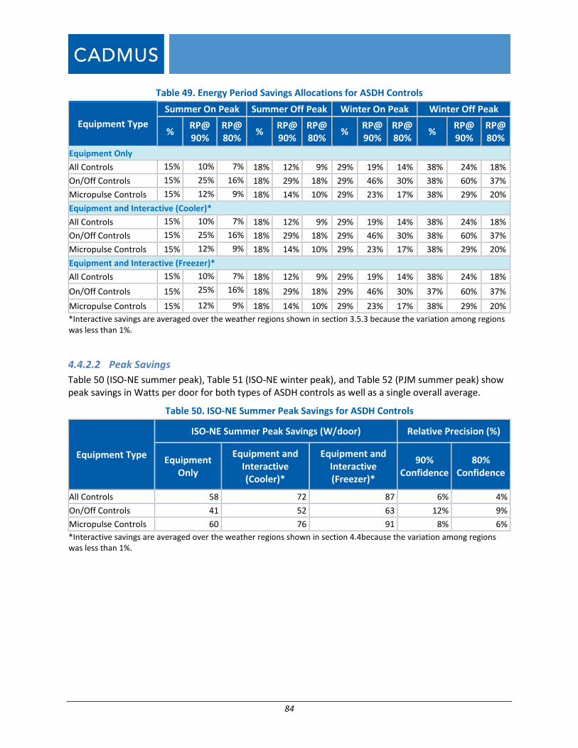
84
Table 49. Energy Period Savings Allocations for ASDH Controls
Equipment Type
Summer On Peak Summer Off Peak Winter On Peak Winter Off Peak
% RP@ 90%
RP@ 80%
% RP@ 90%
RP@ 80%
% RP@ 90%
RP@ 80%
% RP@ 90%
RP@ 80%
Equipment Only
All Controls 15% 10% 7% 18% 12% 9% 29% 19% 14% 38% 24% 18%
On/Off Controls 15% 25% 16% 18% 29% 18% 29% 46% 30% 38% 60% 37%
Micropulse Controls 15% 12% 9% 18% 14% 10% 29% 23% 17% 38% 29% 20%
Equipment and Interactive (Cooler)*
All Controls 15% 10% 7% 18% 12% 9% 29% 19% 14% 38% 24% 18%
On/Off Controls 15% 25% 16% 18% 29% 18% 29% 46% 30% 38% 60% 37%
Micropulse Controls 15% 12% 9% 18% 14% 10% 29% 23% 17% 38% 29% 20%
Equipment and Interactive (Freezer)*
All Controls 15% 10% 7% 18% 12% 9% 29% 19% 14% 38% 24% 18%
On/Off Controls 15% 25% 16% 18% 29% 18% 29% 46% 30% 37% 60% 37%
Micropulse Controls 15% 12% 9% 18% 14% 10% 29% 23% 17% 38% 29% 20%
*Interactive savings are averaged over the weather regions shown in section 3.5.3 because the variation among regions was less than 1%.
4.4.2.2 Peak Savings
Table 50 (ISO-NE summer peak), Table 51 (ISO-NE winter peak), and Table 52 (PJM summer peak) show peak savings in Watts per door for both types of ASDH controls as well as a single overall average.
Table 50. ISO-NE Summer Peak Savings for ASDH Controls
Equipment Type
ISO-NE Summer Peak Savings (W/door) Relative Precision (%)
Equipment Only
Equipment and Interactive (Cooler)*
Equipment and Interactive (Freezer)*
90% Confidence
80% Confidence
All Controls 58 72 87 6% 4%
On/Off Controls 41 52 63 12% 9%
Micropulse Controls 60 76 91 8% 6%
*Interactive savings are averaged over the weather regions shown in section 4.4because the variation among regions was less than 1%.
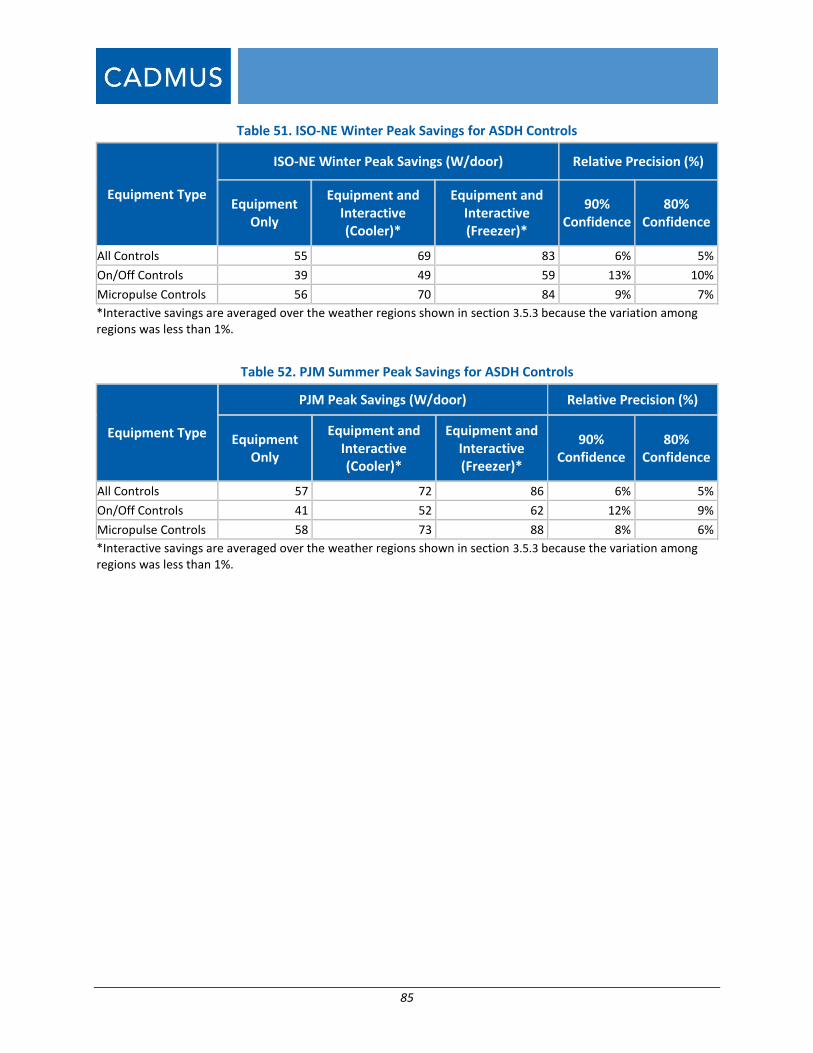
85
Table 51. ISO-NE Winter Peak Savings for ASDH Controls
Equipment Type
ISO-NE Winter Peak Savings (W/door) Relative Precision (%)
Equipment Only
Equipment and Interactive (Cooler)*
Equipment and Interactive (Freezer)*
90% Confidence
80% Confidence
All Controls 55 69 83 6% 5%
On/Off Controls 39 49 59 13% 10%
Micropulse Controls 56 70 84 9% 7%
*Interactive savings are averaged over the weather regions shown in section 3.5.3 because the variation among regions was less than 1%.
Table 52. PJM Summer Peak Savings for ASDH Controls
Equipment Type
PJM Peak Savings (W/door) Relative Precision (%)
Equipment Only
Equipment and Interactive (Cooler)*
Equipment and Interactive (Freezer)*
90% Confidence
80% Confidence
All Controls 57 72 86 6% 5%
On/Off Controls 41 52 62 12% 9%
Micropulse Controls 58 73 88 8% 6%
*Interactive savings are averaged over the weather regions shown in section 3.5.3 because the variation among regions was less than 1%.
86
5 Findings and Recommendations
The evaluation team offers the following findings and recommendations for program administrators,
implementers, and evaluators of these commercial refrigeration measures to improve the energy
savings of installations and the effectiveness of programs.
5.1.1 Key Findings
All three measure provide both energy and peak demand savings.
The evaluated operating parameters and savings results for all measures are similar to the values
currently estimated in the PAs TRMs.
All three measures are unobtrusive and provide reliable savings. There is minimal opportunity for
interference from the customer that could impact performance.
The measures have a wide range of commercial applications. The evaluation team observed
measure installations in coolers and freezers, walk-in spaces, and reach-in cases. The team also
observed measure installations across variety of commercial building types, including small
businesses and large commercial facilities.
The evaluation team observed negligible differences (<1%) in measure performance based on
weather. There is therefore no reason for different performance expectation based on geographic
region.
5.1.2 ECM Retrofits
ECM retrofits reduce operating power by 59% on average compared to baseline SP motors.
Uncontrolled evaporator fan motors operate continuously and therefore adding controls is a good
measure for both annual energy and peak demand savings.
Only two of the observed baseline motors were SP. Implementation contractors confirmed they
are less likely to replace baseline PSC motors because the replacement is less cost-effective
compared to SP replacements. Program administrators that use a blended SP/permanent split
capacitor (PSC) baseline should consider using a SP only baseline.29
The majority of installed motors are rated at 1/15 horsepower, but we observed motors ranging
from 12 Watts (equivalent to 1/62 hp) to 1/4 hp. The average rated horsepower from our sample
was 1/12 hp.
Operating power varies for both baseline SP motors and uncontrolled ECMs. This variation is
caused by multiple factors, including differences in rated motor horsepower and efficiency,
diameter and pitch of attached fans, and airflow restrictions. Cadmus tested the impact of airflow
29 Contractors confirmed SP motors are the predominant equipment used on evaporator fan motors for
commercial refrigeration applications. Since they are less efficient than PSC motors, they are also more likely
to be targeted for upgrades.
87
restrictions on motor power. Refer for Appendix B. Airflow Restriction Testing for the results of
the testing. See Section 3.5.2.1 for more detail on the observed variation in operating power.
The rated horsepower of pre-installation and post-installation motors do not always match. For
example, a 1/15-hp SP motor might be replaced with a 1/20-hp ECM, or vice versa. This is due to
geometrical constraints and equipment availability.
One pre-retrofit small grocery site (Site 27. EF-A: Small Grocery) had uncontrolled SP motors that
exhibited an average run time of 51%. We confirmed that the motors did not have controls but
noted that the power consumption fluctuated rapidly and turned off frequently. This indicated the
motor was malfunctioning, which is expected for a small percentage of baseline condition motors.
5.1.3 Evaporator Fan Controls
Evaporator fan controls reduce run time by 32% compared to fans without controls.
Controlled evaporator fan motors operate more frequently during peak periods than periods of
inactivity, but continue to turn on and off throughout the day and are therefore still a good
measure for peak demand savings.
The average run time for controlled motors varies. This variation is caused by multiple factors,
including the control type (ON/OFF style controls which vary the runtime of the motor, versus
multi-speed controls which vary the speed and runtime of the motor), space temperature settings,
and condition of refrigeration equipment. See Section 3.5.2.1 for more detail on the observed
variation in operating power.
The two types of EF controls (ON/OFF and multi-speed) perform differently. ON/OFF controls
resulted in slightly greater energy and peak demand savings than multi-speed controls.
At two of the sites we included in our analysis, controls were disconnected by the customer.
Future metering studies of controls such as these should include investigations of customer
behavior to understand whether controls are routinely disconnected by the customer, and if so,
the reasons why.
5.1.4 Anti-Sweat Door Heater Controls
ASDH controls reduce run time by 45% compared to door heaters without controls.
Controlled ASDHs operate more frequently during peak periods than periods of inactivity, but
continue to turn on and off throughout the day and are therefore still a good measure for peak
demand savings.
The two types of door heater controls (micropulse and ON/OFF) perform differently. Micropulse
controls resulted in greater energy and peak demand savings than ON/OFF controls.
There is variation in the run time of uncontrolled ASDH due to manual operation. At one site (2.
DH-A: Liquor Store), site personnel manually turned the heaters on and off every night. Through
discussions with contractors, we confirmed this is fairly common operating condition (Section
3.5.2.2).
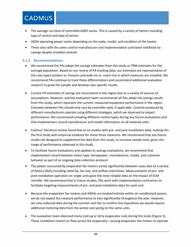
88
The average run time of controlled ASDH varies. This is caused by a variety of factors including
type of control and type of sensor.
ASDH operating power varies depending on the make, model, and condition of the heater.
Three sites with the same control manufacturer and implementation contractor exhibited no
savings despite installed controls.
5.1.5 Recommendations
We recommend the PAs adopt the savings estimates from this study as TRM estimates for the
average population. Based on our review of PA tracking data, our estimates are representative of
the case types (coolers vs. freezers and walk-ins vs. reach-ins) in which measures are installed. We
recommend PAs continue to track these differentiators and recommend additional evaluation
research to grow the sample and develop case-specific results.
Current PA estimates of savings are inconsistent in the region due to a variety of sources of
assumptions. However, and the evaluation team recommends all PAs adopt the savings results
from this study, which represent the current, measured equipment performance in the region.
Estimates between PAs should only vary by controller style, if applicable. Controls produced by
different manufacturers operate using different strategies, which we observed to impact
performance. We recommend sampling different control types during any future evaluations and
that implementers record manufacturer and model information on all metered units.
Cadmus’ literature review found few to no studies with pre- and post-installation data, making this
the first study with empirical evidence for these three measures. We recommend that any future
studies be designed to supplement the data from this study, to increase sample sizes, given the
range of performance observed in this study.
To facilitate future evaluations and updates to savings evaluations, we recommend that
implementers record baseline motor type, horsepower, manufacturer, model, and customer
behavior as part of an ongoing data collection protocol.
The power consumed by evaporator fan motors varied significantly between cases due to a variety
of factors likely including rated hp, fan size, and airflow restrictions. Measurements of pre- and
post-installation operation on single units gave the most reliable data on the impact of ECM
retrofits. We recommend that in future studies, PAs work with implementation contractors to
facilitate targeting measurements of pre- and post-installation data for each unit.
Because the evaporator fan motors and ASDHs are located entirely within air-conditioned spaces,
we do not expect the measure performance to vary significantly throughout the year. However,
we only collected data during the summer and fall; to confirm this hypothesis we would require
additional metering data from the winter and spring on the same units.
The evaluation team observed many iced-up or dirty evaporator coils during the study (Figure 5).
These conditions restrict air flow across the evaporator, causing evaporator fan motors to operate
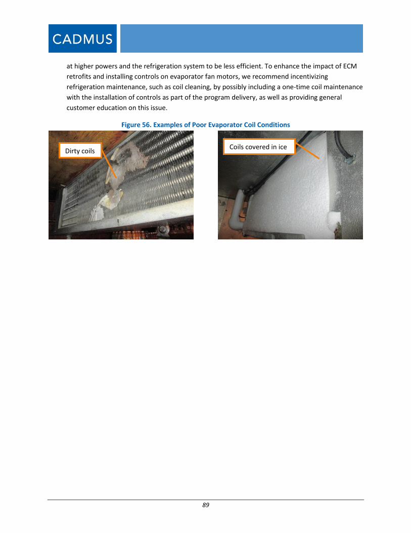
89
at higher powers and the refrigeration system to be less efficient. To enhance the impact of ECM
retrofits and installing controls on evaporator fan motors, we recommend incentivizing
refrigeration maintenance, such as coil cleaning, by possibly including a one-time coil maintenance
with the installation of controls as part of the program delivery, as well as providing general
customer education on this issue.
Figure 56. Examples of Poor Evaporator Coil Conditions
Dirty coils Coils covered in ice
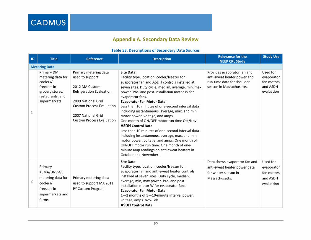
90
Appendix A. Secondary Data Review
Table 53. Descriptions of Secondary Data Sources
ID Title Reference Description Relevance for the NEEP CRL Study
Study Use
Metering Data
1
Primary DMI metering data for coolers/ freezers in grocery stores, restaurants, and supermarkets
Primary metering data used to support: 2012 MA Custom Refrigeration Evaluation 2009 National Grid Custom Process Evaluation 2007 National Grid Custom Process Evaluation
Site Data: Facility type, location, cooler/freezer for
evaporator fan and ASDH controls installed at
seven sites. Duty cycle, median, average, min, max power. Pre- and post-installation motor W for evaporator fans. Evaporator Fan Motor Data: Less than 10 minutes of one-second interval data including instantaneous, average, max, and min motor power, voltage, and amps. One month of ON/OFF motor run time Oct/Nov.
ASDH Control Data:
Less than 10 minutes of one-second interval data including instantaneous, average, max, and min motor power, voltage, and amps. One month of ON/OFF motor run time. One month of one-minute amp readings on anti-sweat heaters in October and November.
Provides evaporator fan and anti-sweat heater power and run-time data for shoulder season in Massachusetts.
Used for evaporator fan motors and ASDH evaluation
2
Primary
KEMA/DNV-GL
metering data for
coolers/
freezers in
supermarkets and
farms
Primary metering data
used to support MA 2011
PY Custom Program.
Site Data: Facility type, location, cooler/freezer for evaporator fan and anti-sweat heater controls installed at seven sites. Duty cycle, median, average, min, max power. Pre- and post-installation motor W for evaporator fans. Evaporator Fan Motor Data: 1—2 months of 5—10-minute interval power, voltage, amps. Nov-Feb.
ASDH Control Data:
Data shows evaporator fan and
anti-sweat heater power data
for winter season in
Massachusetts.
Used for
evaporator
fan motors
and ASDH
evaluation
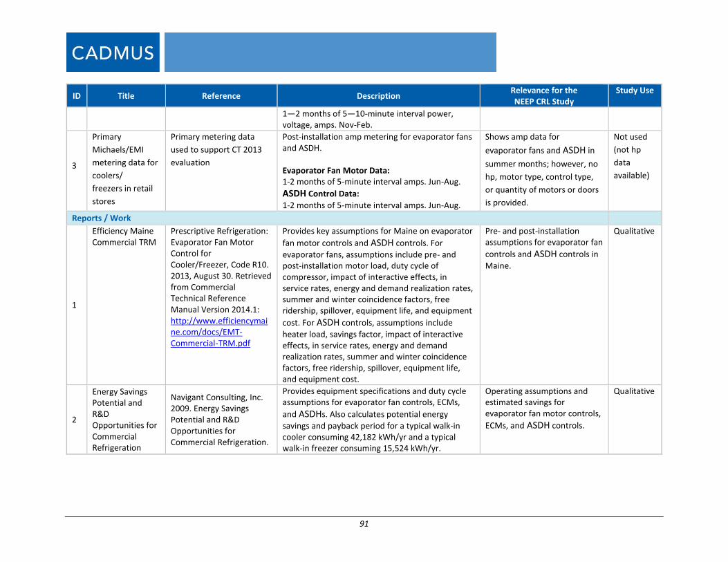
91
ID Title Reference Description Relevance for the NEEP CRL Study
Study Use
1—2 months of 5—10-minute interval power, voltage, amps. Nov-Feb.
3
Primary
Michaels/EMI
metering data for
coolers/
freezers in retail
stores
Primary metering data
used to support CT 2013
evaluation
Post-installation amp metering for evaporator fans and ASDH. Evaporator Fan Motor Data: 1-2 months of 5-minute interval amps. Jun-Aug.
ASDH Control Data:
1-2 months of 5-minute interval amps. Jun-Aug.
Shows amp data for
evaporator fans and ASDH in
summer months; however, no
hp, motor type, control type,
or quantity of motors or doors
is provided.
Not used
(not hp
data
available)
Reports / Work
1
Efficiency Maine Commercial TRM
Prescriptive Refrigeration: Evaporator Fan Motor Control for Cooler/Freezer, Code R10. 2013, August 30. Retrieved from Commercial Technical Reference Manual Version 2014.1: http://www.efficiencymaine.com/docs/EMT-Commercial-TRM.pdf
Provides key assumptions for Maine on evaporator
fan motor controls and ASDH controls. For
evaporator fans, assumptions include pre- and post-installation motor load, duty cycle of compressor, impact of interactive effects, in service rates, energy and demand realization rates, summer and winter coincidence factors, free ridership, spillover, equipment life, and equipment
cost. For ASDH controls, assumptions include
heater load, savings factor, impact of interactive effects, in service rates, energy and demand realization rates, summer and winter coincidence factors, free ridership, spillover, equipment life, and equipment cost.
Pre- and post-installation assumptions for evaporator fan
controls and ASDH controls in
Maine.
Qualitative
2
Energy Savings Potential and R&D Opportunities for Commercial Refrigeration
Navigant Consulting, Inc. 2009. Energy Savings Potential and R&D Opportunities for Commercial Refrigeration.
Provides equipment specifications and duty cycle assumptions for evaporator fan controls, ECMs,
and ASDHs. Also calculates potential energy
savings and payback period for a typical walk-in cooler consuming 42,182 kWh/yr and a typical walk-in freezer consuming 15,524 kWh/yr.
Operating assumptions and estimated savings for evaporator fan motor controls,
ECMs, and ASDH controls.
Qualitative
92
ID Title Reference Description Relevance for the NEEP CRL Study
Study Use
3
EnergyIdeas Clearinghouse Product & Technology Review
EnergyIdeas Clearinghouse. 2008, December. Product and Technology Reviews: Frigitek® Control. Retrieved from EnergyIdeas Clearinghouse: http://www.energyideas.org/documents/Factsheets/PTR/Frigitek-Dec08.pdf
Provides Frigitek manufacturer’s savings claims on evaporator fan motor controls. Also includes assumptions on motor efficiency, rpm, duty cycle, and costs.
Operating assumptions and estimated savings for evaporator fan motor controls.
Qualitative
4
Energy Savings Potential for Commercial Refrigeration Equipment
Arthur D. Little. (1996). Energy Savings Potential for Commercial Refrigeration Equipment.
Provides assumptions for on pre- and post-installation duty cycle for evaporator fan controls and annual savings estimations for evaporator fan
controls and ASDH controls.
Operating assumptions and estimated savings for evaporator fan controls and
ASDH controls.
Qualitative
5
Efficient Evaporator Fan Motors (Shaded Pole to ECM)
Southern California Edison Company. (2007). Efficient Evaporator Fan Motors (Shaded Pole to ECM).
Provides estimated savings and input assumptions for SP to ECM retrofits. Estimated savings and assumptions are provided for coolers and freezers for restaurants and grocery stores.
Operating assumptions and estimated savings for SP to ECM retrofits for restaurants and grocery.
Qualitative
6
Response to questions on Anti-Sweat Heater (ASH) Control Savings Work Paper
Memo between Cadmus and CLEAResult (November 2012). Response to questions on Anti-Sweat Heater (ASH) Control Savings Work Paper
Savings and key assumptions for low temperature
and medium temperature ASDH controls from six
sources. Savings include kWh/linear foot and kW/linear foot. Key assumptions include ASH power and EEER. Savings were calculated for the El Dorado, Arizona, climate zone using 8,760 data.
Key assumptions for ASDH
controls.
Qualitative
7
Field Testing of ECMs for Supermarket Display Cases
Foster-Miller, Inc. 1995. Field Testing of Electronically Commutated Motors for Supermarket Display Cases
Provides energy and demand savings results from field testing of ECMs in a 29-door frozen food case in a 42,000 sq ft supermarket in Menlo Park, California. Measurements were taken over three months before and after the motors were installed.
Energy savings of ECM retrofits from field testing in Menlo Park, California.
Qualitative
93
ID Title Reference Description Relevance for the NEEP CRL Study
Study Use
8
RTF Anti-sweat Heater Controls Workbook v2.0
Regional Technical Forum. 2013, October 9. Commercial: Grocery - Anti-Sweat Heater Controls v2.0. Retrieved from Regional Technical Forum
Provides possible pre- and post-installation energy
consumptions of ASDH controls and explanation of
sources.
Estimated pre- and post-installation energy
consumption data for ASDH
controls.
Qualitative
9
RTF Walk-in Evaporator Fan ECM Motor Controls Workbook v1.2
Regional Technical Forum. 2014, March 19. Commercial: Grocery - Walk-in Evaporator Fan ECM Motor Controllers v1.2. Retrieved from Regional Technical Forum
Provides possible evaporator fan power, run time, EER, and fan speed after installation of controls installed on ECMs and gives explanation of sources.
Key assumptions for evaporator fan controls installed on ECMs.
Qualitative
10
RTF Walk-in Evaporator Fan Shaded Pole Motor Controls Workbook v1.0
Regional Technical Forum. 2012, December 11. Commercial: Grocery - Walk-in Evaporator Fan Shaded Pole Motor Controllers v1.0. Retrieved from Regional Technical Forum
Provides possible evaporator fan motor power, EER, and fan speed after installation of controls on SP motor and gives explanation of sources.
Key assumptions for evaporator fan controls installed on SP motors.
Qualitative
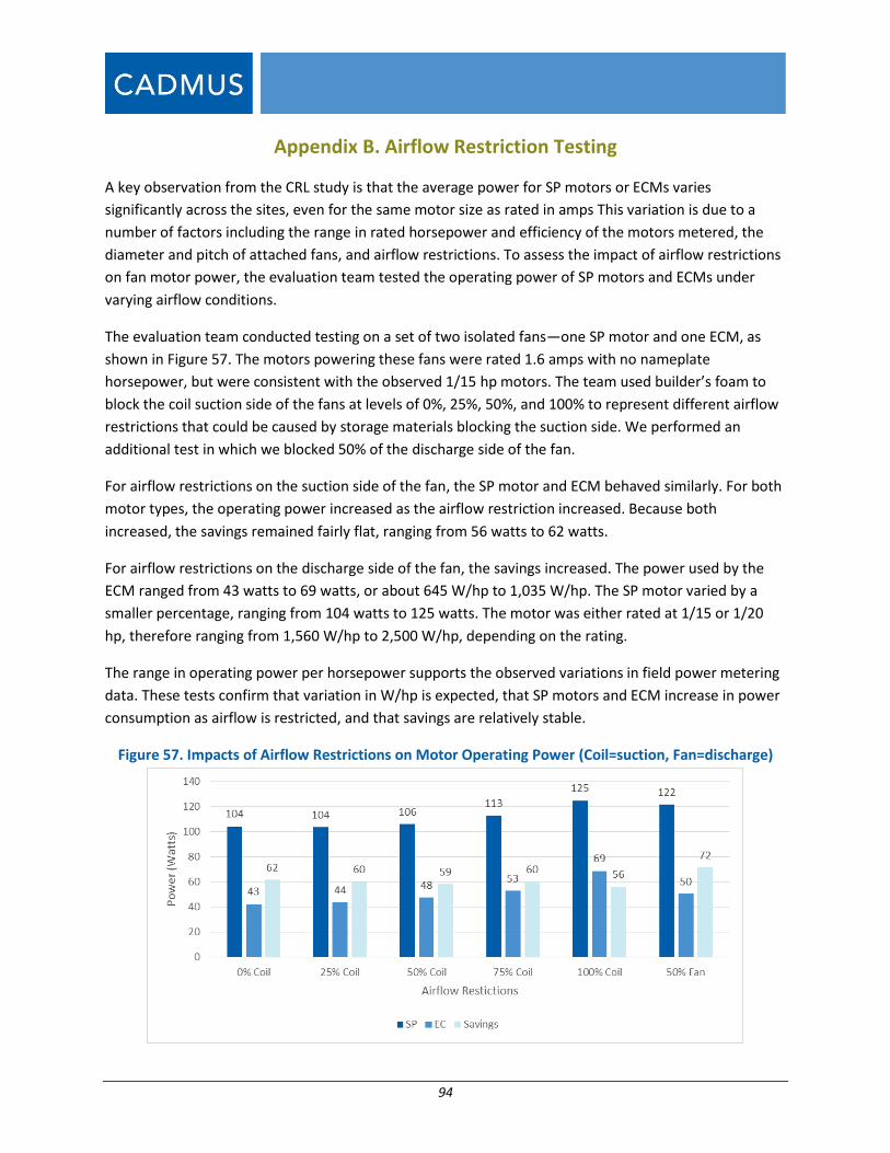
94
Appendix B. Airflow Restriction Testing
A key observation from the CRL study is that the average power for SP motors or ECMs varies
significantly across the sites, even for the same motor size as rated in amps This variation is due to a
number of factors including the range in rated horsepower and efficiency of the motors metered, the
diameter and pitch of attached fans, and airflow restrictions. To assess the impact of airflow restrictions
on fan motor power, the evaluation team tested the operating power of SP motors and ECMs under
varying airflow conditions.
The evaluation team conducted testing on a set of two isolated fans—one SP motor and one ECM, as
shown in Figure 57. The motors powering these fans were rated 1.6 amps with no nameplate
horsepower, but were consistent with the observed 1/15 hp motors. The team used builder’s foam to
block the coil suction side of the fans at levels of 0%, 25%, 50%, and 100% to represent different airflow
restrictions that could be caused by storage materials blocking the suction side. We performed an
additional test in which we blocked 50% of the discharge side of the fan.
For airflow restrictions on the suction side of the fan, the SP motor and ECM behaved similarly. For both
motor types, the operating power increased as the airflow restriction increased. Because both
increased, the savings remained fairly flat, ranging from 56 watts to 62 watts.
For airflow restrictions on the discharge side of the fan, the savings increased. The power used by the
ECM ranged from 43 watts to 69 watts, or about 645 W/hp to 1,035 W/hp. The SP motor varied by a
smaller percentage, ranging from 104 watts to 125 watts. The motor was either rated at 1/15 or 1/20
hp, therefore ranging from 1,560 W/hp to 2,500 W/hp, depending on the rating.
The range in operating power per horsepower supports the observed variations in field power metering
data. These tests confirm that variation in W/hp is expected, that SP motors and ECM increase in power
consumption as airflow is restricted, and that savings are relatively stable.
Figure 57. Impacts of Airflow Restrictions on Motor Operating Power (Coil=suction, Fan=discharge)