Embed Size (px)
Citation preview
COMMISSION INTERNATIONALE
DES GRANDS BARRAGES
Quatorzieme Congres des Grands Barrages Rio de Janeiro, 1982
Q. 54 R. 20
PREDICTION OF LANDSLIDE-GENERATED WATER WAVES(*)
CLIFFORD A. PUGH
Hydraulic Engineer, Hydraulic Structures Section
DAVID W. HARRIS
Civil Enf(ineer, Embankment Dams Sectio n
US BUREAU OF RECLAMATION
USA
INTRODUCTION
Slow moving landslides are common in valleys and canyons where reservoirs are usually located. Under certain conditions, it is possible for a landslide to break away and plunge into the water at high speeds. If this happens, large waves are formed which can create serious problems. Some areas of concern are : (1) loss of life; (2) damage to shoreline structures and boats; (3) overtopping of dams by waves with resulting damage to dams, intake structures, spillways, and powerhouses; (4) failure of dams; (5) upstream flooding due to river blockages; and (6) loss of usage of the water body due to the final position of slide material [ 1].
In 1963 a massive rockslide fell into the reservoir upstream from Vaiont dam in Italy. A wave estimated to be 100 m high spilled over the dam. The disaster resulted in the loss of about 2 600 human lives [2]. Following the
(*) Ca/cul des vagues induites par un glissement de terrain.
283
' Q. 54-R. 20 .,...,
Vaiont dam disaster many researchers began trying to simulate landslidegenerated waves. Empirical methods as well as mathematical and physical models have been used in the simulations.
An assessment -of the magnitude of landslide-generated waves in Bureau of Reclamation reservoirs with potential landslides is important to the safe operation of those reservoirs. Even if the landslides have very little chance of breaking free, it is prudent to estimate the magnitude of landslide-generated waves. If the likelihood of a slide becoming active is considered great enough, measures such as lowering the pool level to prevent dam overtopping for a predicted wave height could be taken to , reduce the hazards.
This paper summarizes the results of a study done by the Bureau of Reclamation on the available empirical methods and the design, construction, t~sting, and results of a physical model study performed on landslidegenerated waves in Morrow Point reservoir. In addition, a numerical model now under development by a contractor to the Bureau of Reclamation is explained. The numerical model should be general enough to apply to a variety of reservoirs and other bodies of water. The results from the physical model study will be used to calibrate and verify the numerical model. Results from previous studies will also be used to verify the numerical model.
HISTORIC OCCURRENCES
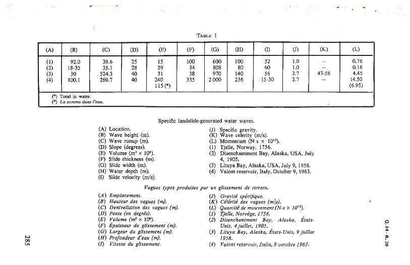
Descriptions of significant historic occurrences of landslide-generated water waves are given in the literature (2, 3, 4]. Accounts of the destruction caused by water waves are given for three specific cases [ 4] in addition to the Vaiont case [2]. Table 1 shows data pertinent to wave prediction.
1. In the winter of 1756 an icefall occurred in Langford, Norway (the J'jelle event). An ice volume of 15 hm3 slid into a fjord generating runups of 40 m on distant shorelines. From the runups, a wave height of 92 m was calculated. Thirty-two persons were killed in the event.
2. An icefall was reported on July 4, 1905, in Disenchantment Bay, Alaska, USA [5]. At a distance of 0.8 km, alder bushes at a height of 33.5 m were broken off. Vegetation was killed at a height of 20 m, 4.8 km -from the slide. At about equal distances in different directions, destroyd alders indicated waves of 18 to 3 5 m.
3. In the Gilbert inlet on the northeast end of Lituya Bay, Alaska, USA, at about 10:16 p.m. local time, July 9, 1958, a "deafening crash" was reported by one witness. A rock prism roughly triangular in cross section and with an estimated volume of 30.6 hm3 [6] slid into the bay generating a large gravity wave with a steep front. This wave was reflected down the bay as a 30-metre-high wave with a crest width of8 to 15 m. Forest cover was stripped l 100 m inland from the high tide line and approximately 0.3 m of soil was
284
,·
N 00 V,
TABLE I
(A) (B) (C) (D) (E) (F) (G) (H) (I) (J)
(I) 92.0 39.6 25 15 100 600 100 52 1.0 (2) 18-35 35.1 28 29 34 808 80 60 1.0 (3) 30 524.3 40 31 38 970 140 56 2.7 (4) 100.1 269.7 40 240 335 2000 236 15-30 2.7
115 (*)
(*) Total in water. (
0) La somme dans l'eau.
(A) Location. (B) Wave height (m). (C) Wave runup (m). (D) Slope (degrees).
Specific landslide-generated water waves.
(J) Specific gravity. (K) Wave celerity (m/ s).
(E) Volume (ml x 106).
(F) Slide thic~ness (m). (G) Slide width (m). (H) Water depth (m). (I) Slide velocity (m/ s).
(L) Momentum (N-s x 1012).
(I) Tjelle, Norway, 1756. (2) Disenchantment Bay, Alaska, USA, July
4, 1905. (3) Lituya Bay, Alaska, USA, July 9, 1958. (4) Vaiont reservoir, Italy, October 9, 1963.
Vagues types produites par un g/issement de terrain.
(A) Emplacement. (B) Hauteur des vagues (m). (C) Denivellation des vagues (m). (D) Pente (en degres). (E) Volume (ml x 106).
(F) Epaisseur du glissement (m). (G) Largeur du glissement (m). (H) Profondeur d'eau (m). (I) Vitesse du glissement.
(J) Gravite specijique. (K) Celerite des vagues (m]s). (L) Quantile de mouvement (N-s x 1012) .
(1) Tjel/e, Norvege, 1756. (2) Disenchantment Bay , Alaska, Etats
Unis, 4 jui/let, 1905. (3) Lituy a Bay , Alaska, Etats-Unis, 9 juil/et
1958. (4) Vaiont reservoir, Jtalie, 9 octobre 1963.
(K) (L)
- 0.76 - 0.18
43-58 4.45 - 14.50
(6.95)
Q.54-R.20
removed up to the wave trimline. An area of 10 km2 was destroyed with 3 hm3
of soil eroded. Two boats sank and two persons were killed. 4. One of the most damaging reservoir disasters of all time occurred on
October 9, 1963, at Vaiont dam in Italy [2]. During the night a rockslide in excess of 240 hm3 slid at a velocity of approximately 30 m per second into the .,.. reservoir. A 100-m wave overtopped the dam and maintained a height of 70 m 1.6 km downstream obliterating the town of Longavone. Loss of life was esti-mated to be 2 600 persons.
r---\ I I
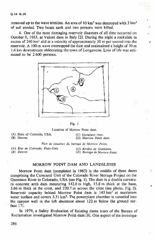
+--- ~-----J_ Fig. I
Location of Morrow Point dam.
(A) State of Colorado, USA. (B) Denver.
(C) Gunnison river. (D) Morrow Point dam.
Plan de situation du barrage de Morrow Point.
(A) Etat de Colorado, Etats-Unis. ( C) Riviere de Gunnison. (B) Denver. (D) Barrage de Morro w Point.
MORROW POINT DAM AND LANDSLIDES
Morrow Point dam (completed in 1963) ii. the middle of three dams comprising the Curecanti Unit of the Colorado River Storage Project on the Gunnison River in Colorado, USA (see Fig. 1). The dam is a double curvature concrete arch dam measuring 142.6 m high, 15.8 m thick at the base, 3.66 m thick at the crest, and 220.7 m across the crest (see photo, Fig. 2). Reservoir capacity behind Morrow Point dam is 145 hm3 at maximum water surface and covers 3.31 km 2
• The powerplant chamber is tunneled into the canyon wall in the left abutment about 122 m below the ground surface [7].
In 1979, a Safety Evaluation of Existing dams team of the Bureau of Reclamation investigated Morrow Point dam (8]. One aspect of the investiga-
286
Q. 54 -R. 20
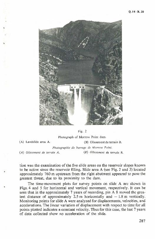
Fig. 2
Photograph of Morrow Point dam.
(A) Landslide area A. (B) Glissement de terrain B.
Photographie du barrage de Morrow Point.
(A) Glissement de terrain A. (B) Glissement de terrain B.
tion was the examination of the five slide areas on the reservoir slopes known to be active since the reservoir filling. Slide area A (see Fig. 2 and 3) located approximately 760 m upstream from the right abutment appeared to pose the greatest threat, due to its proximity to the dam.
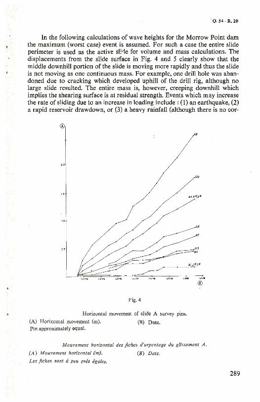
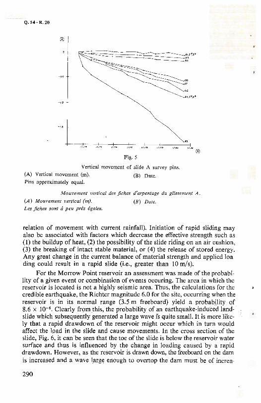
The time-movement plots for survey points on slide A are shown in Figs. 4 and 5 for horizontal and vertical movement, respectively. It can be seen that in the approximately 7 years of recording, pin A-8 moved the greatest distance of approximately 2.5 m horizontally and - 1.8 m vertically. Monitoring points for slide A were analyzed for displacements, velocities, and accelerations. The linear variation of displacement with respect to time for all points plotted indicates a constant velocity. Thus for this case, the last 7 years of data collected show no acceleration of the slide.
287
Q.54-R.20
It 0000 -IOOO·!OO 0 MlOO zooo >000 .. ,oo
(fNt}
-,oo -no Q !00 IOO 000 ,zoo '""" (melrH)
L -4 -10 4 e 12 t6 ZO
I I t,,,1,,,l,11l111l111I (fHtl
·• • • •
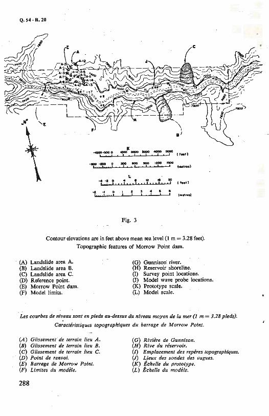
Fig. 3
Contour elevations are in feet above mean sea level (1 m = 3.28 feet).
Topographic features of Morrow Point dam.
(A) Landslide area A. (B) Landslide area B. (C) Landslide area C. (D) Reference point. (E) Morrow Point dam. (F) Model limits.
(G) Gunnison river. (H) Reservoir shoreline. (I) Survey point locations. (J) Model wave probe locations. (K) Prototype scale. (L) Model scale.
Les courbes de niveau sont en pieds au-dessus du niveau moyen de la mer (I m = 3.28 pieds).
Caracteristiques topographiques du barrage de Morrow Point.
(A) Glissement de terrain lieu A. (B) Glissement de terrain lieu B. ( C) Glissement de terrain lieu C. (D) Point de renvoi. (E) Barrage de Morrow Point. (F) Limites du modele.
288
(G) Riviere de Gunnison. (H) Rive du reservoir. (I) Emplacement des reperes topographiques. (J) Lieux des sondes des vagues. (K) Echelle du prototype. (L) Echelle du modele.
. Q,-54 - R. 20
In the following calculations of wave heights for the Morrow Point dam the maximum (worst case) event is assumed. For such a case the entire slide perimeter is used as the active sli-ie for volume and mass calculations. The displacements from the slide surface in Fig. 4 and 5 clearly show that the middle downhill portion of the slide is moving more rapidly and thus the slide is not moving as one continuous mass. For example, one drill hole was abandoned due to cracking which developed uphill of the drill rig, although no large slide resulted. The entire mass is, however, creeping downhill which implies the shearing surface is at residual strength. Events which may increase the rate of sliding due to an increase in loading include : (1) an earthquake, (2) a rapid reservoir drawdown, or (3) a heavy rainfall (although there is no cor-
@
20
15
1.0
05
Fig. 4
Horizontal movement of slide A survey pins.
(A) Horizontal movement (m). Pin approximately equal.
(B) Date.
AB
®
Mouvement horizontal des fiches d'arpentage du g/issement A.
(A) Mouvement horizontal (m). (B) Date.
Les fiches son/ d peu pres egales.
289
Q.54-R.20
@
- OS
-10
-15
A8
® Fig. 5
Vertical movement of slide A survey pins.
(A) Vertical movement (m). (B) Date. Pins approximately equal.
Mouvement vertical des fiches d'arpentage du glissement A.
(A) Mouvement vertical (m) . (B) Date.
Les fiches sont a peu pres egales.
relation of movement with current rainfall). Initiation of rapid sliding may also be associated with factors which decrease the effective strength such as (I) the buildup of heat, (2) the possibility of the slide riding on an air cushion, (3) the breaking of intact stable material, or (4) the release of stored energy. Any great change in the current balance of material strength and applied loading could result in a rapid slide (i.e., greater than IO m/s).
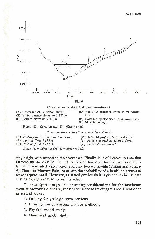
For the Morrow Point reservoir an assessment was made of the probability of a given event or combination of events occuring. The area in which the reservoir is located is not a highly seismic area. Thus, the calculations for the credible earthquake, the Richter magnitude 6.0 for the site, occurring when the reservoir is in its normal range (3.5 m freeboard) yield a probability of 8.6 x 10- 6 • Clearly from this, the probability of an earthquake-induced landslide which subsequently generated a large wave i's quite small. It is more likely that a rapid drawdown of the reservoir might occur which in turn would affect the load in the slide and cause movements. In the cross section of the slide, Fig. 6, it can be seen that the toe of the slide is below the reservoir water surface and thus is influenced by the change in loading caused by a rapid drawdown. However, as the reservoir is drawn down, the freeboard on the dam is increased and a wave large enough to overtop the dam must be of increa-
290
Q.54-R.20
2500
2400
2300
] I
LI.I 2200
2100
2000
-300 -200 -100 0
D-(m)
100
Fig. 6
200 300
Cross section of slide A (facing downstream).
F
400 500 600
(A) Centerline of Gunnison river. (D) Point 10 projected from 15 m downs-(B) Water surface elevation 2 182 m. tream. (C) Bottom elevation 2 073 m. (E) Point 6 projected from 15 m downstream.
(F) Slide boundary. Notes: E = elevation (m), D = distance (m).
Coupe au /ravers du glissement A (vue d'aval).
(A) Thalweg de la riviere de Gunnison. (D) Point JO projete de 15 ma !'aval. (B) Cote de l'eau 2 182 m. (E) Point 6 projete de 15 m a /'aval. (C) Cote du fond 2 973 m. (F) Limite du glissement.
Notes: E = elevation (m), D = distance (m).
sing height with respect to the drawdown. Finally, it is of interest to note that historically no dam in the United States has ever been overtopped by a landslide-generated water wave, and only two worldwide (Vaiont and Pontessi). Thus, for Morrow Point reservoir, the probability of a landslide-generated wave is quite small. However, as stated previously it is prudent to investigate any damaging event to assess its effect.
To investigate design and operating considerations for the maximum event at Morrow Point dam, subsequent work to investigate slide A was done in several areas :
1. Drilling for geologic cross sections.
2. Investigation of existing analysis methods.
3. Physical model study.
4. Numerical model study.
291

Q. 54-R. 20
EMPIRICAL RELATIONS
There are a number of methods suggested for the calculation of landslide-generated water waves. Slingerland and Voight [ 4] consider the methods of (1) the Noda simulation of a vertically falling box or a horizontally moving wall; (2) the empirical equations ofKamphuis and Bowering; (3) an empirical equation, derived by Slingerland and Voight, based on the Waterways Experiment Station Libby dam model [ 10] and verified with historical inciden!s; and (4) the Raney and Butler modification of vertically averaged nonlinear wave equations l 1]. The theoretical wave height produced by Morrow Point landslide A was estimated with all of these methods. However, methods 1 and 3 yielded lower values, which were felt to be reasonable and the discussion will be limited to these two methods. The methods will be discussed in the following two sections.
NODA.
Noda [9] simulated a landslide using a box with a base dimension of A and height greater than the depth of the water, d, dropped into the water at velocity vn(t}. The generated wave has a maximum height ofry. Additional assumptions involved in the derivation are :
1. The slide volume is small compared to the water volume.
2. The velocity-time history of the box is known. 3. The fluid is incompressible, its motion irrotational, and the linearized
equations of surface gravity waves are applicable. 4. The horizontal fluid velocity under the box is not a function of z, the
direction of the box drop. 5. Impact phenomena can be ignored. The actual prediction of the maximum wave height is done using charts
prepared by Noda from laboratory tests. The process may be summarized as follows:
1. Compute velocity of slide. A suggested relation [ 4] is :
v = v0 + 2 gs[sin (i}- tan 'Ps cos (i)] (1)
where:
292
v = slide velocity computed as a mass sliding on a plane; v0 = initial slide velocity; g = gravitational constant; s = distance of travel of slide; i = slope angle in degrees;
tan 'Ps = coefficient of dynamic sliding friction including pore pressure and roughness effects. May be taken as 0. 25 ± 0.12.
2. Compute Froude number = v/(gd)0·5• (2)
Q. 54-R. 20
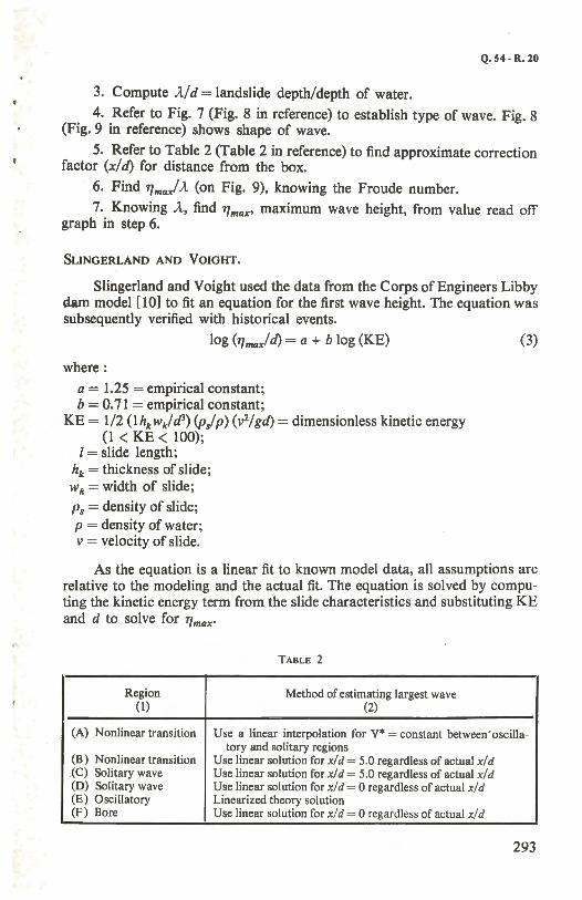
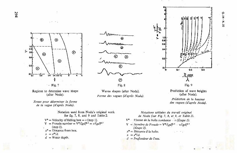
3. Compute J./d = landslide depth/depth of water.
4. Refer to Fig. 7 (Fig. 8 in reference) to establish type of wave. Fig. 8 (Fig. 9 in reference) shows shape of wave.
5. Refer to Table 2 (Table 2 in reference) to find approximate correction factor (xi d) for distance from the box.
6. Find Tfmaxf J. (on Fig. 9), knowing the Froude number.
7. Knowing J., find T/max• maximum wave height, from value read off graph in step 6.
SLINGERLAND AND VOIGHT.
Slingerland and Voight used the data from the Corps of Engineers Libby dam model [ 10] to fit an equation for the first wave height. The equation was subsequently verified with historical events.
log (TJma)d) =a+ blog (KE) (3)
where:
a= 1.25 = empirical constant; b = 0. 71 = empirical constant;
KE= 1/2 (lhk wk/c/3) (p.f p) (v2/gd) = dimensionless kinetic energy (1 < KE < 100);
I= slide length; hk = thickness of slide; wk= width of slide;
Ps = density of slide; p = density of water; v = velocity of slide.
As the equation is a linear fit to known model data, all assumptions are relative to the modeling and the actual fit. The equation is solved by computing the kinetic energy term from the slide characteristics and substituting KE and d to solve for T/max·
TABLE 2
Region Method of estimating largest wave ( I) (2)
(A) Nonlinear transition Use a linear interpolation for v• = constant betwecn·oscilla-tory and solitary regions
(B) Nonlinear transition Use linear solution for x/d = 5.0 regardless of actual x/d _(C) Solitary wave Use linear solution for x/ d = 5.0 regardless of actual x/d (D) Solitary wave Use linear solution for x/d = 0 regardless of actual x/d (E) Osci llatory Linearized theory solution (F) Bore Use linear solution for x/d = 0 regardless of actual x/ d
293
3
t
~
--,···-r
® @
©
'-1 06 OB 10
.A • Fig. 7
®
4 6
® Fig. 8
10,~------------
0.11
0.6
0.4
0.
0.1
g e~ "' 2 !? S?
;. -. -
0.2
.ll..mS!..x. A
Fig. 9
0.3
Regions to determine wave shape (after Noda).
Waves shapes (after Noda). Prediction of wave heights (after Noda). Forme des vagues (d'apres Noda}.
Zones pour determiner la forme de la vague (d'apres Noda).
Notation used from Noda's original work for fig. 7, 8, and 9 and Table 2.
V* = Velocity of falling box= v (step 1). V = Froude number= V*/(gd)0·5 = v/(gd)0· 5
(step 2). x* = Distance from box. X = x*/d. d = Water depth.
Prediction de la hauteur des vagues (d'apres Noda).
Notations uti/isees du travail original de Noda (sur Fig. 7, 8, et 9, et Table 2).
V* = Vitesse de la boite tombante = · v (Et ape 1).
V = Nombre de Froude = V*/(gd)0·5 = v/(gd)0·5
(Etape 2). x* = Distanced la boite. X = x*/d. d = Profondeur de l'eau.
•
•
•
----------------------.....:Q.54-R.20
The model was constructed to an undistorted scale of I : 250. The model topography was formed by projecting contour maps onto plywood with a ver-
MORROW POINT CALCULATIONS •
The approximation for slide A used the dimensions of width equal to 381 m, a thickness of 30 m, a length of 381 m, and a slide distance of 195 m. A velocity estimate was computed from equation (I) based on the slide distance. The resulting velocity is linearly proportional to slide distance and thus care must be exercised in choosing this parameter. For these calculations the distance was based on the distance the toe had to travel before coming to rest slightly beyond the centerline of the reservoir bottom. By making this assumption, a velocity estimate of 32.91 mis was used. Note that the requirements for rapid sliding discussed previously influence the velocity and these velocities are a maximum value. The volume of 4.35 hm3 was computed from the above dimensions. Reservoir depth at the slide is approximately 110 m. The angle of inclination o( the slide is 30° and the dynamic friction term, tan <fJs, was taken as 0.25. For the upper bound velocity estimate, the Noda and Slingerland and Voight prediction methods resulted in 10.36- and 15.25-m wave heights, respectively. For a lower velocity estimate, values of 10.36 and 5. 79 m were computed. For the higher velocity, the two methods were assumed to bound the actual case. The subsequent physical model showed the wave height to be slightly higher than the Slingerland and Voight predictions. It is interesting to note that for velocities in this range, the Noda graphs (derived from model studies) are asymptotic and thus yield the same wave height.
PHYSICAL MODEL STUDY
A physical model study was used at the Bureau of Reclamation Hydraulics Laboratory to accurately determine the characteristics of waves generated by landslides in Morrow Point reservoir. The model simulates the effect of topography of the reservoir as well as bends and other geometric features. Downstream effects are also simulated. Empirical relations and numerical methods can be verified using the model results .
THE MODEL.
The model included 5.3 km of reservoir and 1.3 km of the canyon downstream from the dam. Three landslide areas designated " A ", " B ", and " C " were studied. Fig. 3 is a plan of the reservoir area showing the location of the landslides and the model limits.
295
Q. 54- R. 20
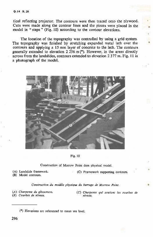
tical reflecting projector. The contours were then traced onto the plywood. Cuts were made along the contour lines and the pieces were placed in the model in " steps " (Fig. 10) according to the contour elevations.
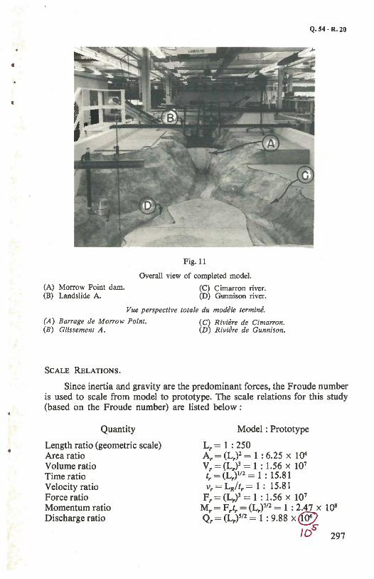
The location of the topography was controlled by using a grid system. The topography was finished by stretching expanded metal lath over the contours and applying a 15 mm layer of concrete to the lath. The contours generally extended to elevation 2 256 m (*). However, in the areas directly across from the landslides, contours extended to elevation 2 3 77 m. Fig. 11 is a photograph of the model.
Fig. 10
Construction of Morrow Point dam physical model.
(A) Landslide framework. (B) Model contours.
(C) Framework supporting contours.
Construction du mode/e physique du barrage de Morrow Point.
(A) Charpente du glissement. (B) Courbes de niveau.
( C) Charpente qui soutient !es courbes de niveau.
(*) Elevations are referenced to mean sea level.
296
•
•
•
•
(A) Morrow Point dam. (B) Landslide A.
Fig. II
Overall view of completed model.
(C) Cimarron river. (D) Gunnison river.
Vue perspective totale du modele termine.
(A) Barrage de Morrow Point. (C) Riviere de Cimarron. (B) Glissement A. (D) Riviere de Gunnison.
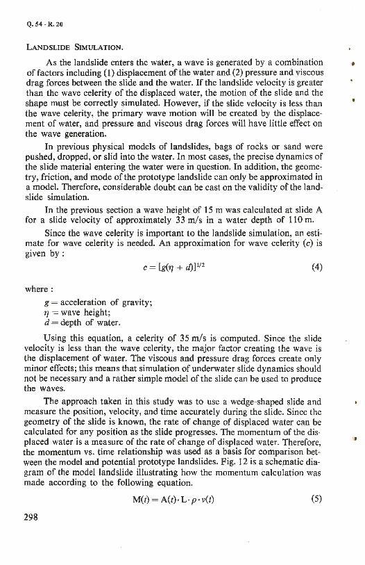
SCALE RELATIONS.
Q.54-R.20
Since inertia and gravity are the predominant forces, the Froude number is used to scale from model to prototype. The scale relations for this study (based on the Froude number) are listed below :
Quantity
Length ratio (geometric scale) Area ratio Volume ratio Time ratio Velocity ratio Force ratio Momentum ratio Discharge ratio
Model : Prototype
L, = 1 : 250 A,= (L,)2 = 1 : 6.25 x 10⁴ V, = (L,)3 = 1 : 1.56 x 10⁷
t, = (L,)112 = 1 : 15.81 v, = LR/t, = 1: 15.81
F, = (L,)3 = 1 : 1.56 x 10⁷
M, = F,t, = (L,)712 = 1 : 2.47 x 10⁸
Q, = (L,)512 = 1 : 9.88 x (@2 IDs 297
Q. 54-R.20
LANDSLIDE SIMULATION.
As the landslide enters the water, a wave is generated by a combination • of factors including (1) displacement of the water and (2) pressure and viscous drag forces between the slide and the water. If the landslide velocity is greater than the wave celerity of the displaced water, the motion of the slide and the shape must be correctly simulated. However, if the slide velocity is less than the wave celerity, the primary wave motion will be created by the displace-ment of water, and pressure and viscous drag forces will have little effect on the wave generation.
In previous physical models of landslides, bags of rocks or sand were pushed, dropped, or slid into the water. In most cases, the precise dynamics of the slide material entering the water were in question. In addition, the geometry, friction, and mode of the prototype landslide can only be approximated in a model. Therefore, considerable doubt can be cast on the validity of the landslide simulation.
In the previous section a wave height of 15 m was calculated at slide A for a slide velocity of approximately 33 m/s in a water depth of 110 m.
Since the wave celerity is important to the landslide simulation, an estimate for wave celerity is needed. An approximation for wave celerity (c) is given by:
C = [g(I] + d) ]112
where:
g = acceleration of gravity; '1J = wave height; d = depth of water.
(4)
Using this equation, a celerity of 35 m/s is computed. Since the slide velocity is less than the wave celerity, the major factor creating the wave is the displacement of water. The viscous and pressure drag forces create only minor effects; this means that simulation of underwater slide dynamics should not be necessary and a rather simple model of the slide can be used to produce the waves.
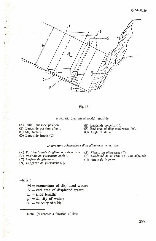
The approach taken in this study was to use a wedge-shaped slide and measure the position, velocity, and time accurately during the slide. Since the geometry of the slide is known, the rate of change of displaced water can be calculated for any position as the slide progresses. The momentum of the displaced water is a measure of the rate of change of displaced water. Therefore, the momentum vs. time relationship was used as a basis for comparison between the model and potential prototype landslides. Fig. 12 is a schematic diagram of the model landslide illustrating how the momentum calculation was made according to the following equation.
M(t) = A(t)· L· p · v(t) (5)
298
'
Q.54-R.20
Fig. 12
Schematic diagram of model landslide.
(A) Initial landslide position. (B) Landslide position after I. (C) Slip surface. (D) Landslide length (L).
(E) Landslide velocity (v). (F) End area of displaced water (A). (G) Angle of slope.
Diagramme schematique d'un glissement de terrain.
(E) Vitesse du glissement ( V). (A) Position initiale du glissement de terrain. (B) Position du g/issement apres t. ( C) Surface de glissement.
(F) Extremite de la zone de l'eau deplucee (G) Angle de la pente.
(D) Longueur du glissement (L).
where:
M = momentum of displaced water; A = end area of displaced water; L = slide length; p = density of water; v = velocity of slide.
Note : (1) denotes a function of time.
299
Q. 54-R.20
The model landslide is scaled to match the length of the prototype landslide and enters the water at the same angle. The volume of the model landslide is designed to match the prototype volume when it reaches the bottom of the • valley. The angle of the front face of the model landslide determines the volu-me.
In addition to the rate of displacement of water by the slide and total volume of displacement by the slide, the momentum vs. time relationship for the prototype slides and model slides was matched. To compute the momentum for the prototype slide equation (1) was used incrementally for the total displaced position as discussed in the previous section. Once the toe had reached the bottom of the reservoir, an overrun of material from the uphill portion of the slide was estimated. This produced a momentum vs. time graph which was S-shaped.
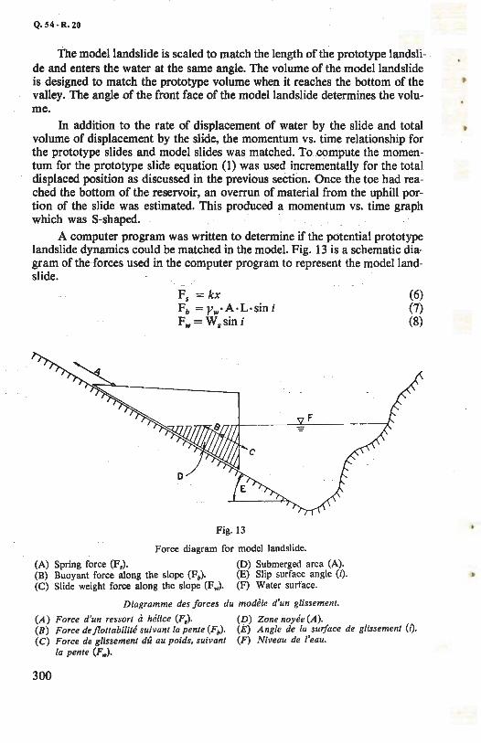
A computer program was written to determine if the potential prototype landslide dynamics could be matched in the model. Fig. 13 is a schematic diagram of the forces used in the computer program to represent the model landslide.
(A) Spring force (F,).
Fs = kx F b = y.., · A· L · sin i F.., = Wssin i
Fig. 13
Force diagram for model landslide.
(B) Buoyant force along the slope (Fb). (D) Submerged area (A). (E) Slip surface angle (i). (F) Water surface. (C) Slide weight force along the slope (F..,).
Diagramme des forces du modele d'un glissement.
(6) (7) (8)
(A) Force d'un ressort a he/ice (F,). (D) Zone noyee (A). (B) Force deflottabilite suivant la pente (Fb). (E) Angle de la surface de glissement (i). ( C) Force de glissement du au poids, suivant (F) Niveau de l'eau.
la pente (F..,).
300
'
t
where:
k = spring constant. x = spring stretch. L = slide length. i = slip surface angle.
w. = weight of the slide.
Q. 54-R.20
Yw = specific weight of water. A = submerged end area of slide. F s = spring force. Fb = buoyant force along slope. F w = slide weight force along slope.
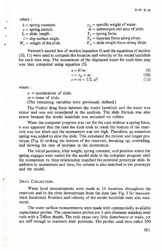
Newton's second law of motion (equation 9)-and the equations of motion (10, 11) were used to compute the location and velocity of the model landslide for each time step. The momentum of the displaced water for each time step was then computed using equation (5).
a=F/m (9) v = v0 + at (10) s = vt + 1/2 at2 (11)
where:
a = acceleration of slide. m = mass of slide. (The remaining variables were previously defined.)
The friction drag force between the model landslide and the water was minor and was not considered in the analysis. The slide friction was also minor because the model landslide was mounted on rollers.
When the computer program was run for the case without a spring force, it was apparent that the time the slide took to reach the bottom of the reservoir was too short and the momentum was too high. Therefore, an extension spring was added to slow the slide. This simulated the thinner and longer prototype (Fig. 6) striking the bottom of the reservoir, breaking up, overriding, and slowing the rate of increase in the momentum.
The initial position, slide weight, spring constant, and position where the spring engages were varied for the model slide in the computer program until the momentum vs. time relationship matched the potential prototype slide. In addition to momentum and time, the volume is also matched in the prototype and the model.
DATA COLLECTION.
Water level measurements were made at 14 locations throughout the reservoir and in the river downstream from the dam (see Fig. 3 for measurement locations). Position and velocity of the model landslide were also measured.
The water surface measurements were made with commercially available capacitance probes. The capacitance probes are 3-mm-diameter stainless steel rods with a Teflon sheath. The rods cause very little disturbance or wake, yet are stiff enough to maintain their positions. The probes used were either 300
301
Q.54 - R. 20
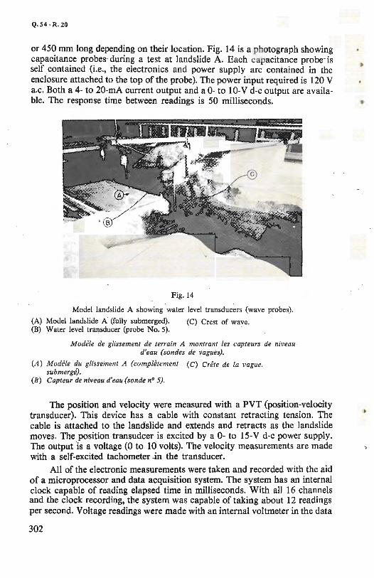
or 450 mm long depending on their location. Fig. 14 is a photograph showing capacitance probes during a test at landslide A. Each capacitance probe is self contained (i.e., the electronics and power supply are contained in the enclosure attached to the top of the probe). The power input required is 120 V a.c. Both a 4- to 20-mA current output and a 0- to 10-V d-c output are available. The response time between readings is 50 milliseconds.
Fig. 14
Model landslide A showing water level transducers (wave probes).
(A) Model landslide A (fully submerged). (C) Crest of wave. (B) Water level transducer (probe No. 5).
Modele de glissement de terrain A montrant /es capteurs de niveau d'eau (sondes de vagues).
(A) Modele du glissement A (completement (C) Crete de la vague. submerge).
(B) Capteur de niveau d'eau (sonde n° 5).
The position and velocity were measured with a PVT (position-velocity transducer). This device has a cable with constant retracting tension. The cable is attached to the landslide and extends and retracts as the landslide moves. The position transudcer is excited by a 0- to 15-V d-c power supply. The output is a voltage (Oto 10 volts). The velocity measurements are made with a self-excited tachometer in the transducer.
All of the electronic measurements were taken and recorded with the aid of a microprocessor and data acquisition system. The system has an internal clock capable of reading elapsed time in milliseconds. With all 16 channels and the clock recording, the system was capable of taking about 12 readings per second. Voltage readings were made with an internal voltmeter in the data
302
•
Q. 54-R. 20
(A)
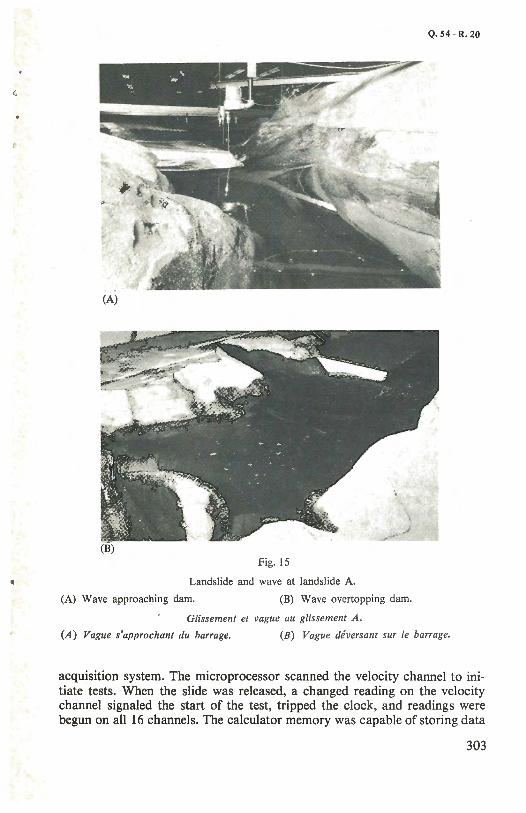
Fig. 15
Landslide and wave at landslide A.
(A) Wave approaching dam. (B) Wave overtopping dam.
G/issement et vague au g/issement A.
(A) Vague s'approchant du barrage. (B) Vague deversant sur le barrage.
acquisition system. The microprocessor scanned the velocity channel to initiate tests. When the slide was released, a · changed reading on the velocity channel signaled the start of the test, tripped the clock, and readings were begun on all 16 channels. The calculator memory was capable of storing data
303
Q.54-R.20
for about 20 seconds; the data were then stored on magnetic disk and this cycle of data recording and storage continued until the test was terminated. A 4-second gap in the data occurred while the data were being stored on disk; however, the data of primary interest were obtained in the first 20 seconds.
The PVT and water level transducers were calibrated before testing. All of the instruments demonstrated excellent linearity between output voltage and reading. The calibrations were checked throughout the testing program to ensure that the calibration coefficients did not drift. It was found that a buildup on the Teflon sheath caused the calibration coefficients to drift if the probes were left in the water. Therefore, the probes were cleaned every day prior to testing. This stabilized the calibration. Checks on the calibration coefficients indicated changes of less than 5 percent.
TEST RESULTS.
The primary data consisted of water level recordings and position and velocity measurements of the landslides. The position and velocity readings were converted to slide momentum by consideration of the slide geometry. A range of tests were run at each landslide location. Fig. 15 shows a test at landslide A. The full-scale wave overtopping the dam would be 20 m high.
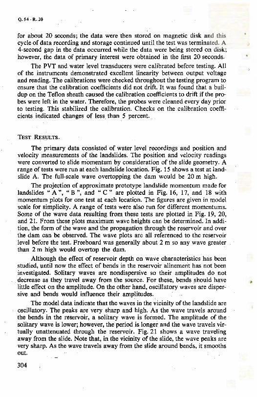
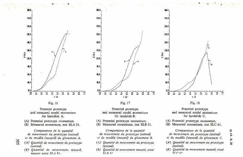
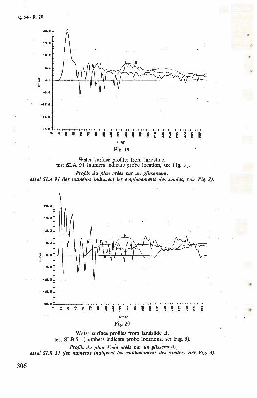
The projection of approximate prototype landslide momentum made for landslides " A ", " B ", and " C " are plotted in Fig. 16, 17, and 18 with momentum plots for one test at each location. The figures are given in model scale for simplicity. A range of tests were also run for different momentums. Some of the wave data resulting from these tests are plotted in Fig. 19, 20, and 21. From these plots maximum wave heights can be determined. In addition, the form of the wave and the propagation through the reservoir and over the dam can be observed. The wave plots are all referenced to the reservoir level before the test. Freeboard was generally about 2 m so any wave greater than 2 m high would overtop the dam.
Although the effect of reservoir depth on wave characteristics has been studied, until now the effect of bends in the reservoir alinement has not been investigated. Solitary waves are nondispersive so their amplitudes do not decrease as they travel away from the source. For these, bends should have little effect on the amplitude. On the other hand, oscillatory waves are dispersive and bends would influence their amplitudes.
The model data indicate that the waves in the vicinity of the landslide are oscillatory. The peaks are very sharp and high. As the wave travels around the bends in the reservoir, a solitary wave is formed. The amplitude of the solitary wave is lower; however, the period is longer and the wave travels virtually unattenuated through the reservoir. Fig. 21 shows a wave traveling away from the slide. Note that, in the vicinity of the slide, the wave peaks are very sharp. As the wave travels away from the slide around bends, it smooths out.
304
• • JIU
278.8
141.B
118.8
111!.B
!SU
J; - 118.8
!U
Ii.I
t(sl
Fig. 16
Potential prototype and measured model momentum
for landslide A.
(A) Potential prototype momentum. (B) Measured momentum, test SLA 91.
Comparaison de la quantile de mouvement du prototype (estime)
et du modele (mesure) du glissement A.
(A) Quantile de mouvement du prototype (estime).
(B) Quantile de mouvement mesure, mesure essai Sl,A 91 .
me
278.8
14li
1111.B
1111.B
ISB.B
J; - ,211.e
!ll.i
Ii.I
:u
t(sl
Fig. 17
Potential prototype and measured model momentum
for landslide B.
(A) Potential prototype momentum. (B) Measured momentum, test SLB 51.
Comparaison de la quantile de mouvement du prototype (estime)
et du mode/e (mesure) du glissement B.
(A) Quantile de mouvement du prototype (estime).
(B) Quantile de mouvement mesure, essai ST.R \' I
"
278.B
118.8
118.8
1111.B
!SU
l - ,211.1
!Ill
11!.i
tW
Fig. 18
Potential prototype and measured model momentum
for landslide C .
(A) Potential prototype momentum. (B) Measured momentum, test SLC 61.
Comparaison de la quantile de mouvement du prototype (estime)
et du modele (mesure) du glissement C.
(A) Quantile de mouvement du prototype (estime).
(B) Quantile de mouvement mesure, essai .<:rr1.1
Q. 54- R.20
.... 3
IS. e
.... s.e
3 ... :!:
-5. .
-1B. 0
-15- a
-2B." m ~ il: ~ m ., ; ., m ., m ., m ; ~ " m " m " m
"' " ~ N .. " .. ~ ~ . " " i!l " N N N ..
t.-CS>
Fig. 19
Water surface profiles from landslide, test SLA 91 (numers indicate probe location, see Fig. 3).
Profils du plan crees par un glissement, essai SLA 91 (/es numeros indiquent /es emplacements des sondes, voir Fig. 3) .
.... 15.0
,._.
s..
:l "-. :!:
-5..
- 1B. B
-is. e
-20. e
" ~ il: " " " !li "' " "' ~ " " " " " m ~
.. Ill I . "' " ~ ~ ~ "' ~ " .; ~ . " N N N
t.-(e)
Fig. 20
Water surface profiles from landslide B, test SLB 51 (numbers indicate probe locations, see Fig. 3).
Projils du plan d'eau crees par un glissement,. essai SLB 51 (/es numeros indiquent /es emplacements des sondes, voir Fig. 3).
306
•
Q.54-R.20
20.. 12
15..
, ... 5. •
:l ... ±
-5..
-10. 0
- 15. 0
1:.-(9)
Fig. 21
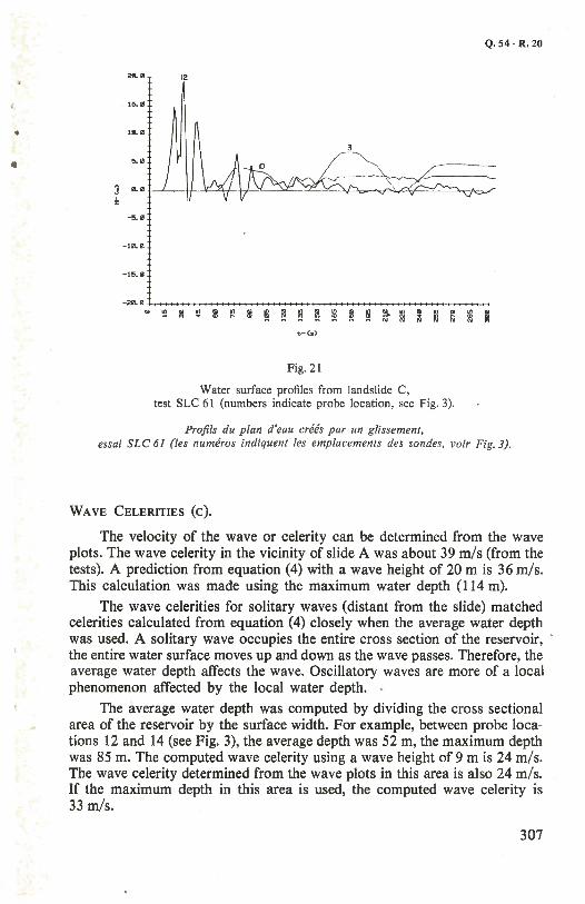
Water surface profiles from landslide C, test SLC 61 (numbers indicate probe location, see Fig. 3).
Projils du plan d'eau crees par un glissement, essai SLC 61 (/es numeros indiquent /es emplacements des sondes, voir Fig. 3).
WAVE CELERITIES (c).
The velocity of the wave or celerity can be determined from the wave plots. The wave celerity in the vicinity of slide A was about 39 mis (from the tests). A prediction from equation (4) with a wave height of 20 m is 36 m/s. This calculation was made using the maximum water depth (114 m).
The wave celerities for solitary waves (distant from the slide) matched celerities calculated from equation (4) closely when the average water depth was used. A solitary wave occupies the entire cross section of the reservoir, the entire water surface moves up and down as the wave passes. Therefore, the average water depth affects the wave. Oscillatory waves are more of a local phenomenon affected by the local water depth. .
The average water depth was computed by dividing the cross sectional area of the reservoir by the surface width. For example, between probe locations 12 and 14 (see Fig. 3), the average depth was 52 m, the maximum depth was 85 m. The computed wave celerity using a wave height of 9 m is 24 m/s. The wave celerity determined from the wave plots in this area is also 24 m/ s. If the maximum depth in this area is used, the computed wave celerity is 33 m/s.
307
Q.54 · R. 20
VOLUME OF WATER 0VERTOPPING THE DAM.
The water overtopping the dam was captured in the downstream channel J
and the volume measured. The volume overtopping due to a slide at location A was 619 000 m3• This is about 14 percent of the slide volume. If it is assu-med that most of the water overtops the dam during the 40 seconds of the main wave, the average discharge during the overtopping is 14 200 m3
/ s. The volume of water overtopping the dam as a result of a slide at loca
tion B was about 243 000 m3• This reduces to an average of 2 800 m3/ s over the 80-second dam overtopping period. The volume is about 7 percent of the total slide volume.
Waves in the river downstream from the dam were bore waves. A slide at location A results in a 7-metre-high wave in the river (Fig. 19). The wave celerity in the river was about 15 m/s. The wave in the river due to a slide at location B was about 4 m high and the wave celerity was about 11 m/s. The still water depth in the river before tests was about 9 m.
WAVE HEIGHT VS. MOMENTUM.
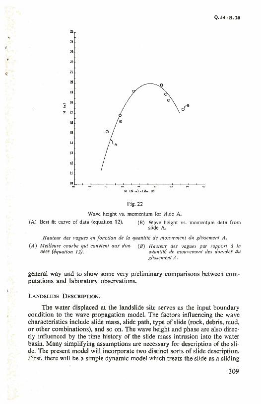
Fig. 22 is a plot of wave height at probe No. 3 vs. maximum slide momentum at slide A. The wave height increases with increasing momentum up to a certain point then decreases with added momentum. A curve was fitted to the data in the form of a parabola (equation 12).
where: I Ac-Ml 2. 1 H=B-
H = 77 = wave height (m). A = momentum at B (N-s). B = maximum wave height (m). C = constant. M = momentum (N-s).
For the data at slide A the results for the " best fit " curve are :
A= 4.61 x 10¹⁰ B = 20 C = 1.18 x 10² 1
(12)
This equation illustrates that a relatively large wave can be generated by a slide of lower velocity. If the landslide momentum is only one-third of the optimum momentum the wave height would still be 11 m at the dam, as opposed to a 20-m wave at the optimum momentum. Data from landslides B and C also show a drop in wave height at the dam for high momentums.
NUMERICAL MODEL
At the time this paper is being prepared, the numerical model is still under development. Nevertheless, it is of interest to describe the model in a
308
•
(
Q.54 - R.20
25
24
23
22
21
21! 0
19
18 0
~ (jB :,: 17
16
15
14
13
12
11
lB
M (N-e) )(10e 10
Fig. 22
Wave height vs. momentum for slide A.
(A) Best fit curve of data (equation 12). (B) Wave height vs . momentum data from slide A.
Ha uteur des vagues en fonction de la quantile de mouvement du g/issement A.
(A) Meilleure courbe qui convient aux donmies (equation 12).
(B) Hauteur des vagues par rapport ci la quantile de mouvement des donnees du glissement A.
general way and to show some very preliminary comparisons between computations and laboratory observations.
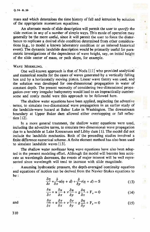
LANDSLIDE DESCRIPTION.
The water displaced at the landslide site serves as the input boundary condition to the wave propagation model. The factors influencing the wave characteristics include slide mass, slide path, type of slide (rock, debris, mud, or other combinations), and so on. The wave height and phase are also directly influenced by the time history of the slide mass intrusion into the water basin. Many simplifying assumptions are necessary for description of the slide. The present model will incorporate two distinct sorts of slide description. First, there will be a simple dynamic model which treats the slide as a sliding
309
Q. 54-R.20
mass and which determines the time history of fall and intrusion by solution of the appropriate momentum equations.
An alternate mode of slide description will permit the user to specify the slide motion in any of a number of simple ways. This mode of operation may generally be the more useful, since it will permit the user to force the disturbance to replicate a desired slide condition determined from other considerations (e.g., to model a known laboratory condition or an inferred historical event). The dynamic landslide description would be primarily useful for parametric investigations of the dependence of wave height, say, on initial height of the slide center of mass, or path slope, for example.
WAVE MODELING.
One well-known approach is that of Noda [ 11] who provided analytical and numerical results for the cases of waves generated by a vertically falling box and by a horizontally moving piston. Linear wave theory was used, and the solution was developed for one-dimensional propagation in water of constant depth. The present necessity of considering two-dimensional propagation over very irregular bathymetry would lead to an impractically cumbersome and costly model were this approach to be followed here.
The shallow water equations have been applied, neglecting the advective terms, to simulate two-dimensional wave propagation in an earlier study of the landslide-wave hazard at Baker Lake in Washington. The downstream boundary at Upper Baker dam allowed either overtopping or full reflection [ 12].
In a more general treatment, the shallow water equations were used, including the advective terms, to simulate two-dimensional wave propagation due to a landslide at Lake Koocanusa and Libby dam [ 1]. The model did not include the landslide mechanics. Both of the preceding studies involved a finite difference numerical scheme. A finite element method has also been used to simulate landslide waves [13].
The shallow water nonlinear long wave equations have also been adopted in the present modeling effort. Although the model will become less accurate as wavelength decreases, the events of major interest will be well represented since wavelength will tend to increase with slide magnitude.
Assuming hydrostatic pressure, the depth-averaged continuity equation and equations of motion can be derived from the Navier-Stokes equations to ~= .
877 8 8 8t + 8x u(77 + d) + 8y v(77 + d) = S (13)
8u 8u 8u 877 - + u - + v-+ g- + F = 0 8 t 8x 8y 8x x
(14)
and 8y 8v 8v 877 -_-+ u-,-+ v-+ g-+ F =0 /:it bx 8y 8y Y
(15)
310
_)
where:
t = time; x, y = horizontal axes;
• "I = surface displacement;
Q. 54 - R.20
u, v = depth averaged velocities in the x and y directions, respectively; < d = still water depth;
S = a sink-source term, positive for source; g = acceleration of gravity;
Fx, FY= components of bottom friction stress per unit mass.
The effect of the Coriolis force is entirely negligible for flow in a relatively small region. The bottom friction stress is obtained from :
gu(u2 + v2)112 (ry + d)C 2 (16)
where C is the Chezy coefficient. The drag between the intruding mass and the fluid will be considered in subsequent work, somewhat along the lines of Raney and Butler.
An explicit finite-difference scheme is used to convert the above partial differential equations into numerical form. An economical scheme [ 14] is used in which all values of the two-dimensional flow components, including surface elevations, velocities, and friction coefficients, are stored in onedimensional vectors the sizes of which are equal to the number of computational grid points. Grid points over land areas will not consume computer memory with this special treatment, and the computation time can be reduced for most applications.
NUMERICAL EXPERIMENT.
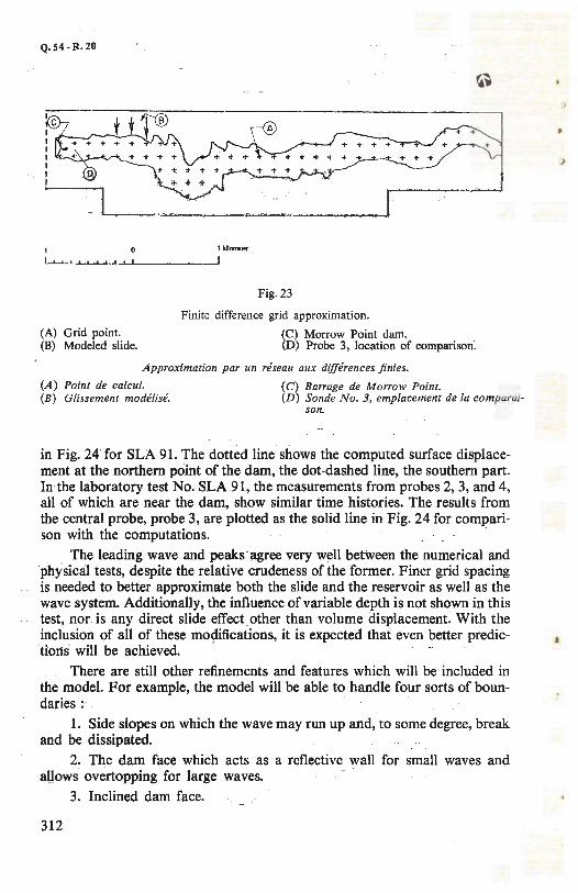
A preliminary version of the numerical model has been exercised to simulate laboratory test No. SLA 91. A 6 x 32 point grid with a uniform step size of 152 m was set up to cover the Morrow Point reservoir area (Fig. 23). In this simulation, the still water depth was set to a constant value of 91 m. Morrow Point dam is located at the west end of the study area as shown in the figure. The time history of the intruding slide volume was recorded during the
• laboratory test and is input to the numerical model as a simple time dependent mass displacement. The width of the slide in the laboratory was L52 m, or 381 m in prototype scale. The intruded mass was modeled by an even distribution to three grid points as indicated by the arrows in Fig. 23. The width of the model slide is thus about 457 m in this numerical experiment, or about 20 percent greater than actual.
RESULTS AND DISCUSSION.
Morrow Point dam is represented by two grids in this preliminary test. The computed surface displacements, H, at these two grid points are plotted
311
Q. 54-R. 20
(A) Grid point. (B) Modeled slide.
1knom!!ter
Fig. 23
Finite difference grid approximation.
(C) Morrow Point dam. {D) Probe 3, location of comparison'.
Approximation par un reseau aux dijferences finies.
(A) Point de ca/cul. {C) Barrage de Morrow Point. (B) G/issement modelise. (D) Sande No. 3, emplacement de la comparai-
son.
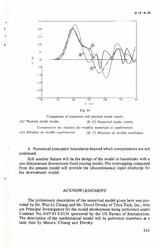
in Fig. 24 for SLA 91. The dotted line shows the computed surface displacement at the northern point of the dam, the dot-dashed line, the southern part. In the laboratory test No. SLA 91, the measurements from probes 2, 3, and 4, all of which are near the dam, show similar time histories. The results from the central probe, probe 3, are plotted as the solid line in Fig. 24 for comparison with the computations.
The leading wave and peaks agree very well between the numerical and physical tests, despite the relative crudeness of the former. Finer grid spacing is needed to better approximate both the slide and the reservoir as well as the wave system. Additionally, the influence of variable depth is not shown in this test, nor is any direct slide effect other than volume displacement. With the inclusion of all of these modifications, it is expected that even better predictions will be achieved.
There are still other refinements and features which will be included in the model. For example, the model will be able to handle four sorts of boundaries :
1. Side slopes on which the wave may run up and, to some degree, break and be dissipated.
2. The dam face which acts as a reflective wall for small waves and allows overtopping for large waves.
3. Inclined dam face.
312
l
t
•
25
20
15
10
5
E 0
I
- 5
-10
- 15
- 20
- 250
t, I ' I
f
,/ l
} _,,,/'
15 30
I I
~\ \
45
t (s)
Fig. 24
60 75
Comparison of numerical and physical model results.
(A) Physical model results. (B, C) Numerical model results.
Comparaison des resultats des mode/es numerique et experimental.
Q.54-R.20
90
(A) Resultats du mode/e experimental. (B, C) Resultats du mode/e numerique.
4. Numerical truncation boundaries beyond which computations are not continued.
Still another feature will be the design of the model to handshake with a one-dimensional downstream flood routing model. The overtopping computed from the present model will provide the (discontinuous) input discharge for the downstream model.
ACKNOWLEDGMENT
The preliminary description of the numerical model given here was provided by Dr. Wen-Li Chiang and Mr. David Divoky of Tetra Tech, Inc., who are Principal Investigators for the model development being performed under Contract No. 0-07-81-S 0134 sponsored by the US Bureau of Reclamation. The description of the mathematical model will be published elsewhere at a later date by Messrs. Chiang and Divoky.
313
Q. 54- R.20
REFERENCES
Ll] RANEY, D. C. and BUTLER, H. L. - "A NumericalModel for Predicting the Effects of Landslide Generated Water Waves ", US Army Engi-neers Waterways Experiment Station Research Report No. H-75-1, " 1975.
L2] JANSEN, R. B. - Dams and Public Safety, US Bureau of Reclamation Technical Publication, Denver, Colorado, 1980.
l3] DAVIDSON, D. D. and McCARTNEY, B. L. -" Water WavesGenerated by Landslides in Reservoirs", Journal of the Hydraulics Division, ASCE, Vol. 101, No. HYD-12, Proc. Paper 11791, pp. 1484-1501, December 1975.
[4] SLINGERLAND, R. L. and VOIGHT, B. - "Occurrences,properties, and predictive models of landslide generated water waves", Rocks/ides and Avalanches, Vol. 2, Elsevier Science Publishing, 1979.
[5] TARR, R. S. - "The Yakutnt Bay Region, Alaska; physiography and glacite geology", US Geological Survey, Prof. Paper 64, 1909.
[6] MILLER, D. J. - "Giant waves in Lituya Bay, Alaska", US Geological Survey, Prof. Paper, 35406. 1960.
[7] - Project Data, USBR Technical Publication, Denver, Colorado, 1981.
[8] - Evaluation Report for Morrow Point dam, Colorado River Storage Project, Upper Colorado Region, USBR. SEED Report, 1979.
[9] NODA, E. - "Water Waves Generated by Landslide", Journal of the Waterways, Harbors, and Coastal Engineering Division, Proceedings of the American Society of Civil Engineers, Vol. 96, No. WW 4, pp. 835-855, November 1970.
[10] DAVIDSON, D. D. and WHALEN, R. W. - "Potential Landslide Generated Waterwaves, Libby dam and Lake Kookanusa, Montana", Technical Report No. H 074-15, US Army Engineers Waterways Experiment Station, Vicksburg, Mississippi, 1974.
[11] NODA, E. - "Theory of Water Waves Generated by a Time-Dependent Boundary Displacement", Technical Report HEL 16-5, Universitv of California, Berkeley, California, iv+ 225 pp., 1969.
[12] Tetra Tech., Inc., "Estimation of Water Wave Heights at Baker Lake Resulting from Possible Landslides from Mt. Baker", Report TC-628, for Puget Sound Power and Light Company, 1975.
[13] KouTITAS, C. G. - "Finite Element Approach to Waves Due to Landslides", Journal of the Hydraulics Division, ASCE Journal 103 (HY 9), Proc. Paper 13218, 1021-1029, 1977.
314
Q.54-R.20
[14] CHIANG, W.-L. - "Tide-lnquced Currents in Harbors of Arbitrary Sha-t pe ", Ph. D. dissertation, University of Southern California,
ix+ 194 pp., 1980.
SUMMARY
In this paper landslide-generated wave predictions are discussed. Three methods are used for the predictions : (I) empirical relations, (2) a physical model, and (3) a numerical model. All results are compared using topographic features and physical dimensions from the Morrow Point reservoir. A 6-to 20-m-high wave is predicted for a rapid slide 750 m from the dam with all methods used.
The empirical methods used in the study are the Noda method and the Slingerland and Voight equation. Both yield approximately the same results with the Slingerland and Voight equation giving slightly smaller results than the model results.
A physical model was constructed to represent the Morrow Point reservoir and simufate three landslides. The landslides accurately model the total displacement of water and the momentum of water displaced by the slide. An electronic measurement system to accurately track the slide and waves throughout the reservoir as well as downstream of the dam was used.
A numerical (computer) technique is being developed to model general cases. Once verified with the physical model results and other available data, the code may be used to solve general cases. With this technique, landslidegenerated water waves can be investigated for reservoirs. The results can be used for design or operational purposes.
RESUME
.1 Dans cette etude, on discute du calcul des vagues induites par des glisse-ments de terrain. II ya trois methodes: (a) !es relations empiriques, (b) un modele physique, et (c) un modele numerique. On compare tous Jes resultats en utilisant !es caracteristiques topographiques et Jes dimensions physiques de la retenue de Morrow Point. Avec toutes Jes methodes utilisees, un glissement rapide de terrain situe a 7 50 m en amont du barrage conduit a prevoir une vague de 6 a 20 m de hauteur.
Les methodes empiriques qu'on a utilisees dans l'etude sont la methode Noda et !'equation de Slingerland et Voight. Les deux methodes donnent a peu pres Jes memes resultats, !'equation de Slingerland et Voight donnant cependant des resultats un peu plus faibles que ceux resultant des modeles.
315
Q.54- R. 20
Un modele physique a ete construit pour representer la retenue de Morrow Point et pour simuler trois glissements de terrain. Les glissements entrainent exactement le deplacement d'eau et la quantite de mouvement. On a utilise un systeme de mesures electroniques pour suivre exactement le glissement et les vagues dans tout le reservoir et egalement en aval du' barrage.
On est en train de mettre au point une technique numerique (avec un ordinateur) pour modeliser tous Jes cas. Quand on aura verifie Jes resultats
· avec le modele physique et d'autres donnees, on pourra utiliser le code dans tous !es cas. Avec cette technique on peut etudier !es glissements de terrain des reservoirs. On peut en utiliser !es resultats au stade du projet ou de !'exploitation.
316
Bureau t::4' Ji\.e~lm!iat-ion HYDRAULICS BRANCH
..