Commodity Options - PMC Derivatives

c24_1 04/28/2008 570

CHAPTER 24Commodity Options

Carol AlexanderChair of Risk Management and Director of Research

ICMA CentreUniversity of Reading

Aanand VenkatramananDoctoral Researcher

ICMA CentreUniversity of Reading

There are three reasons to trade commodity options: diversification, hedg-ing, and speculation. Options are included in investment portfolios be-

cause they have a limited upside or downside, compared with futures.Commodity options provide diversification because they have low correla-tions with equities and bonds. For that reason it is optimal to diversify byadding commodity options to standard portfolios despite their being riskyinstruments.

Risk managers use commodity options to hedge price risk. For instance,calendar spreads can be used to protect producers in a market that tends toswing between backwardation and contango. Average price options (wherethe payoff depends on the difference between some average of underlyingprices and the option strike) are also popular for risk management becausethey are much cheaper than standard options—yet they still allow the pur-chaser to secure supplies at a fixed price.

Speculators use options as highly leveraged bets on price direction. Forinstance, a U.S. calendar spread call on the difference between the one-month futures price and the three-month futures price is a bet that futureswill move to stronger backwardation at some time before the option’s ex-piry. At exercise the purchaser receives a long position on the one-month

570

c24_1 04/28/2008 571

futures and a short position on the three-month futures, at their prevailingmarket prices.

To buy an option is to be long volatility. Hence commodity options canalso be used to speculate on volatility and to hedge volatility risk. All com-modity prices are volatile, some more than others. Agriculturals tend tohave the lowest volatilities, generally only around 30% to 50% but metalsand energy have much higher volatility. For instance, the volatility of on-peak spot electricity prices in the United States was almost 200% in 2005.

This chapter provides a survey of the market for commodity options, theproducts that are commonly traded and the models that we can use to priceand hedge commodity options.

COMMODITY OPTIONS MARKETS

The volume of exchange-traded options on commodities has grown steadilysince the first contracts were introduced in the late 1980s. NYMEX andCOMEX are the most active platforms for trading, mostly in different typesof U.S. options on energy and metals futures. In 2006 a total of 60 millioncommodity options contracts were traded on the Nymex and Comex ex-changes, over 25% of the total volume traded on commodity futures con-tracts (see Exhibit 24.1).

0

50

100

150

200

250

300

1994 1995 1996 1997 1998 1999 2000 2001 2002 2003 2004 2005 2006

Options

Futures

EXHIBIT 24.1 NYMEX Futures and Options Trading Volume

Commodity Options 571

c24_1 04/28/2008 572

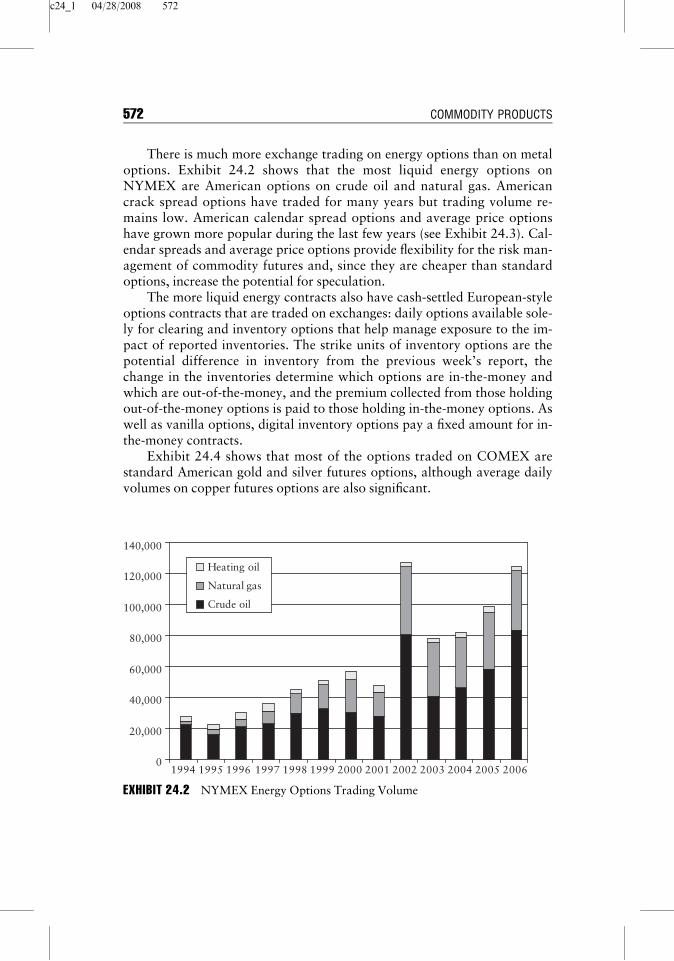
There is much more exchange trading on energy options than on metaloptions. Exhibit 24.2 shows that the most liquid energy options onNYMEX are American options on crude oil and natural gas. Americancrack spread options have traded for many years but trading volume re-mains low. American calendar spread options and average price optionshave grown more popular during the last few years (see Exhibit 24.3). Cal-endar spreads and average price options provide flexibility for the risk man-agement of commodity futures and, since they are cheaper than standardoptions, increase the potential for speculation.

The more liquid energy contracts also have cash-settled European-styleoptions contracts that are traded on exchanges: daily options available sole-ly for clearing and inventory options that help manage exposure to the im-pact of reported inventories. The strike units of inventory options are thepotential difference in inventory from the previous week’s report, thechange in the inventories determine which options are in-the-money andwhich are out-of-the-money, and the premium collected from those holdingout-of-the-money options is paid to those holding in-the-money options. Aswell as vanilla options, digital inventory options pay a fixed amount for in-the-money contracts.

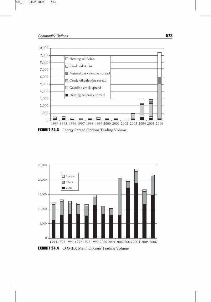
Exhibit 24.4 shows that most of the options traded on COMEX arestandard American gold and silver futures options, although average dailyvolumes on copper futures options are also significant.

0

20,000

40,000

60,000

80,000

100,000

120,000

140,000

1994 1995 1996 1997 1998 1999 2000 2001 2002 2003 2004 2005 2006

Heating oil

Natural gas

Crude oil

EXHIBIT 24.2 NYMEX Energy Options Trading Volume

572 COMMODITY PRODUCTS

c24_1 04/28/2008 573

0

1,000

2,000

3,000

4,000

5,000

6,000

7,000

8,000

9,000

10,000

Heating oil Asian

Crude oil Asian

Natural gas calendar spread

Crude oil calendar spread

Gasoline crack spread

Heating oil crack spread

2006200520042003200220012000199919981997199619951994

EXHIBIT 24.3 Energy Spread Options Trading Volume

0

5,000

10,000

15,000

20,000

25,000

Copper

Silver

Gold

2006200520042003200220012000199919981997199619951994

EXHIBIT 24.4 COMEX Metal Options Trading Volume


c24_1 04/28/2008 574

Two other large exchanges specialize in options on futures of agricul-turals such as dairy products, cocoa, coffee, sugar, soybean products, corn,wheat, live cattle, and lean hogs. These are the CME group (created by tacmerger of Chicago Mercantile Exchange (CME) and the Chicago Board ofTrade (CBOT)) and the main commodity options exchange outside the U.S.,Euronext.Liffe.

Hence the major commodities exchanges all trade in options on futuresof the same maturity as the option, and not in options on spot prices. Thereare two good reasons for this. First, the no-arbitrage argument that gives theoption price has to be based on the possibility of hedging with a liquid asset,and the futures are usually far more liquid than the spot. Secondly, spotprices are more difficult to model than futures prices because they displaymean reversion that is related to seasonally and long-term economic equilib-ria that equate supply and demand. (For instance, if a Chinese car manufac-turer dramatically increases production of inexpensive cars, the price ofgasoline will increase in the short term but over the longer term more refin-eries would be built to meet the demand for gasoline.) In contrast, a fixed-term futures contract is a martingale under the risk neutral measure.

A variety of commodity options are traded over-the-counter (OTC) andfor these the underlying can be the spot price rather than the futures price.Common products include caps (which provide upside protection), floors(which provide downside protection), and collars (which provide both).Path dependent options such as average price options and barriers, whichare cheaper than standard options, are also traded OTC.

A particularly risky OTC option is the floating strike option. The holderof a floating strike European call contract has the right, but not the obliga-tion, to buy the commodity at the strike price every day during the exercisemonth. The strike price is based on the previous end-of-month price. Theprice of the commodity could change considerably during the exercise month,hence the writers of such options face huge risks. These products are alsodifficult to hedge and so are rather expensive. Nevertheless, the demand forsuch products is considerable and even more complex and risky productssuch as have recently become popular.

HISTORICAL PRICE BEHAVIOR

This section examines the behavior of daily spot and futures prices during2005 and 2006 in five different commodities that have actively traded fu-tures options on U.S. exchanges. These are corn, lean hogs, silver, naturalgas, and electricity. They have been chosen to represent the three mainclasses of commodities: agriculturals, metals, and energy. We demonstrate


c24_1 04/28/2008 575

that the price processes for these five different commodities are remarkablydifferent.

Corn

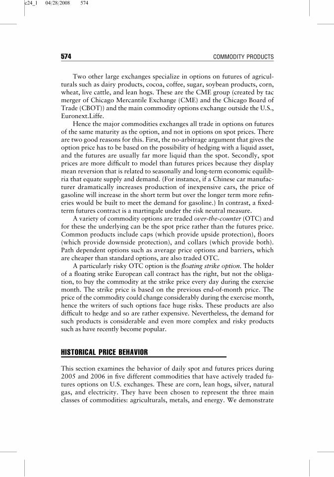
Exhibit 24.5 depicts the spot price on the right hand scale and several fu-tures prices on the left hand scale. Throughout most of 2005 and 2006, themarket was in contango and futures of different maturities are highly corre-lated with each other and with the spot price. Prices can jump at the time ofthe U.S. Department of Agriculture crop production forecasts and in re-sponse to news announcements. A recent example of this was the reactionto President Bush’s announcement of plans to increase ethanol production,clearly visible in January 2007.

Lean Hogs

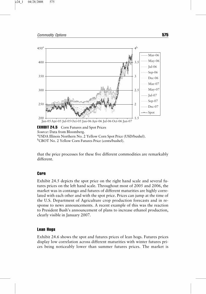
Exhibit 24.6 shows the spot and futures prices of lean hogs. Futures pricesdisplay low correlation across different maturities with winter futures pri-ces being noticeably lower than summer futures prices. The market is

200

250

300

350

400

450a

1.5

2

2.5

3

3.5

4b

Mar-06

May-06

Jul-06

Sep-06

Dec-06

Mar-07

May-07

Jul-07

Sep-07

Dec-07

Spot

Jan-07Jan-05 Jan-06Apr-05 Apr-06Jul-05 Jul-06Oct-05 Oct-06

EXHIBIT 24.5 Corn Futures and Spot PricesSource: Data from Bloomberg.aUSDA Illinois Northern No. 2 Yellow Corn Spot Price (USD/bushel).bCBOT No. 2 Yellow Corn Futures Price (cents/bushel).


c24_1 04/28/2008 576

characterized by a relatively flat demand and an inelastic supply that is setby the farmer’s decision to breed 10-months previously. High prices induceproducers to retain more sows for breeding. This pushes the price evenhigher—and prices tend to peak in the summer months when supply of livehogs is usually at its lowest. Price jumps may correspond to the U.S. De-partment of Agriculture official ‘‘hogs and pigs’’ report on the size of thebreeding herd.

Silver

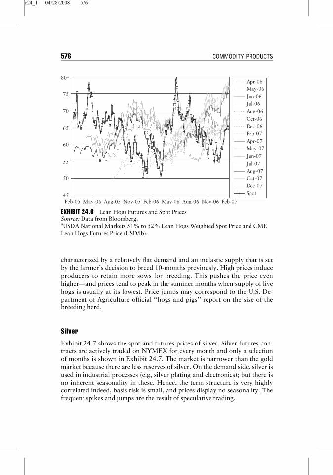
Exhibit 24.7 shows the spot and futures prices of silver. Silver futures con-tracts are actively traded on NYMEX for every month and only a selectionof months is shown in Exhibit 24.7. The market is narrower than the goldmarket because there are less reserves of silver. On the demand side, silver isused in industrial processes (e.g, silver plating and electronics); but there isno inherent seasonality in these. Hence, the term structure is very highlycorrelated indeed, basis risk is small, and prices display no seasonality. Thefrequent spikes and jumps are the result of speculative trading.

45

50

55

60

65

70

75

80a

Apr-06May-06Jun-06Jul-06Aug-06Oct-06Dec-06Feb-07Apr-07May-07Jun-07Jul-07Aug-07Oct-07Dec-07Spot

Nov-06Nov-05 Aug-06Aug-05 May-06May-05Feb-05 Feb-07Feb-06

EXHIBIT 24.6 Lean Hogs Futures and Spot PricesSource: Data from Bloomberg.aUSDA National Markets 51% to 52% Lean Hogs Weighted Spot Price and CMELean Hogs Futures Price (USD/lb).


c24_1 04/28/2008 577

Natural Gas

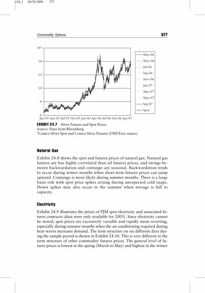
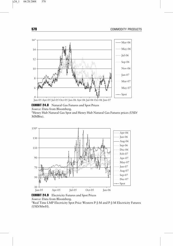
Exhibit 24.8 shows the spot and futures prices of natural gas. Natural gasfutures are less highly correlated than oil futures prices, and swings be-tween backwardation and contango are seasonal. Backwardation tendsto occur during winter months when short-term futures prices can jumpupward. Contango is more likely during summer months. There is a largebasis risk with spot price spikes arising during unexpected cold snaps.Down spikes may also occur in the summer when storage is full tocapacity.

Electricity

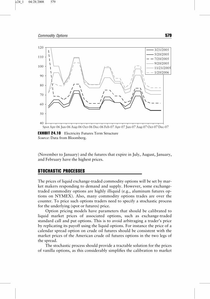
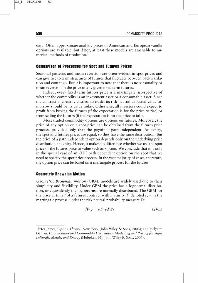
Exhibit 24.9 illustrates the prices of PJM spot electricity and associated fu-tures contracts (data were only available for 2005). Since electricity cannotbe stored, spot prices are excessively variable and rapidly mean reverting,especially during summer months when the air conditioning required duringheat waves increases demand. The term structure on six different days dur-ing the sample period is shown in Exhibit 24.10. This is very different to theterm structure of other commodity futures prices. The general level of fu-tures prices is lowest in the spring (March to May) and highest in the winter

6

8

10

12

14

16a

Mar-06

May-06

Jul-06

Sep-06

Nov-06

Jan-07

Mar-07

May-07

Sep-07

Spot


EXHIBIT 24.7 Silver Futures and Spot PricesSource: Data from Bloomberg.aComex Silver Spot and Comex Silver Futures (USD/Troy ounce).


c24_1 04/28/2008 578

4

6

8

10

12

14

16a

Mar-06

May-06

Jul-06

Sep-06

Nov-06

Jan-07

Mar-07

May-07

Spot


EXHIBIT 24.8 Natural Gas Futures and Spot PricesSource: Data from Bloomberg.aHenry Hub Natural Gas Spot and Henry Hub Natural Gas Futures prices (USD/MMBtu).

30

50

70

90

110

130

150a

Jan-05

Apr-06

Jun-06

Aug-06

Sep-06

Dec-06

Feb-07

Apr-07

May-07

Jun-07

Aug-07

Sep-07

Dec-07

Spot

Jan-06Oct-05Jul-05Apr-05

EXHIBIT 24.9 Electricity Futures and Spot PricesSource: Data from Bloomberg.aReal Time LMP Electricity Spot Price Western P-J-M and P-J-M Electricity Futures(USD/MwH).


c24_1 04/28/2008 579

(November to January) and the futures that expire in July, August, January,and February have the highest prices.

STOCHASTIC PROCESSES

The prices of liquid exchange-traded commodity options will be set by mar-ket makers responding to demand and supply. However, some exchange-traded commodity options are highly illiquid (e.g., aluminum futures op-tions on NYMEX). Also, many commodity options trades are over thecounter. To price such options traders need to specify a stochastic processfor the underlying (spot or futures) price.

Option pricing models have parameters that should be calibrated toliquid market prices of associated options, such as exchange-tradedstandard call and put options. This is to avoid arbitraging a trader’s priceby replicating its payoff using the liquid options. For instance the price of acalendar spread option on crude oil futures should be consistent with themarket prices of the American crude oil futures options in the two legs ofthe spread.

The stochastic process should provide a tractable solution for the pricesof vanilla options, as this considerably simplifies the calibration to market

40

50

60

70

80

90

100

110

120

Aug-06

3/21/20055/20/20057/20/20059/20/200511/21/20051/20/2006

Dec-07Oct-07Spot Apr-06 Jun-06 Aug-07Jun-07Apr-07Feb-07Dec-06Oct-06

EXHIBIT 24.10 Electricity Futures Term StructureSource: Data from Bloomberg.


c24_1 04/28/2008 580

data. Often approximate analytic prices of American and European vanillaoptions are available, but if not, at least these models are amenable to nu-merical methods of resolution.1

Comparison of Processes for Spot and Futures Prices

Seasonal patterns and mean reversion are often evident in spot prices andcan give rise to term structures of futures that fluctuate between backwarda-tion and contango. But it is important to note that there is no seasonality ormean reversion in the price of any given fixed term futures.

Indeed, every fixed term futures price is a martingale, irrespective ofwhether the commodity is an investment asset or a consumable asset. Sincethe contract is virtually costless to trade, its risk-neutral expected value to-morrow should be its value today. Otherwise, all investors could expect toprofit from buying the futures (if the expectation is for the price to rise) orfrom selling the futures (if the expectation is for the price to fall).

Most traded commodity options are options on futures. Moreover, theprice of any option on a spot price can be obtained from the futures priceprocess, provided only that the payoff is path independent. At expiry,the spot and futures prices are equal, so they have the same distribution. Butthe price of a path independent option depends only on the underlying pricedistribution at expiry. Hence, it makes no difference whether we use the spotprice or the futures price to value such an option. We conclude that it is onlyin the special case of an OTC path dependent option on the spot that weneed to specify the spot price process. In the vast majority of cases, therefore,the option price can be based on a martingale process for the futures.

Geometric Brownian Motion

Geometric Brownian motion (GBM) models are widely used due to theirsimplicity and flexibility. Under GBM the price has a lognormal distribu-tion, or equivalently the log returns are normally distributed. The GBM forthe price at time t of a futures contract with maturity T, denoted Ft;T , is themartingale process, under the risk neutral probability measure Q :

dFt;T ¼ sFt;TdWt (24.1)

1Peter James, Option Theory (New York: John Wiley & Sons, 2003); and HelyetteGeman, Commodities and Commodity Derivatives: Modelling and Pricing for Agri-culturals, Metals, and Energy (Hoboken, NJ: John Wiley & Sons, 2005).


c24_1 04/28/2008 581

where the volatility s is constant and W is a Wiener process. Application ofIto’s lemma to the no-arbitrage relationship between spot and futures pricesprovides the following representation for the spot price St:

2

dSt ¼ r� yð ÞStdt þ sStdWt (24.2)

where r is the carry cost (including financing, transportation, storage, insur-ance, etc.) and y is the convenience yield.

It is important to note that equations (24.1) and (24.2) will only beequivalent processes for the market prices of the spot and futures if thefutures is fairly priced; that is, F�t;T ¼ Ft;T . But commodity futures can fallfar below their fair price relative to the spot market price because only aone-way arbitrage is possible (spot commodities cannot be sold short).The deviation of the market price of the futures from its fair price rela-tive to the spot is attributed to the convenience yield, and this is veryuncertain.

Therefore, the equations (24.1) and (24.2) are generally driven by dif-ferent Wiener processes because the uncertainty in the basis appears thespot price, but this never changes the fact that the futures price must be amartingale under the risk-neutral measure.

Spot Price Processes

Spot prices can exhibit mean-reversion and seasonality, and their uncer-tainty includes uncertainty about the basis. This section explains how to ex-tend the process (24.2) to allow for these.

Gibson and Schwartz3 introduced the following two-factor processwith stochastic convenience yield:

dSt ¼ r� yð ÞStdt þ s1StdW1;t

dy ¼ k a� yð Þ � lð Þdt þ s2dW2;t and dW1;t; dW2;t

� �¼ rdt

(24.3)

where k is the rate of mean reversion for the convenience yield, a is themean convenience yield, and l is the convenience yield risk premium.4

2The No-Arbitrage Condition for the Fair Price F�t;T of The Future isF�t;T ¼ Ste

r�yð Þ T�tð Þ.3Rajna Gibson and Eduardo S. Schwartz, ‘‘Stochastic Convenience Yield and thePricing of Oil Contingent Claims,’’ Journal of Finance 45, no. 3 (1990), pp. 959–976.4This allows for risk adjusted drift as convenience yield risk cannot be completelyhedged.


c24_1 04/28/2008 582

The fair value relationship between spot and futures under theseprocesses is given by5

Ft;T ¼ St exp �y1� ekðT�tÞ

kþ At;T

!

(24.4)

where

At;T ¼ r� aþ l

kþ 1

2

s22

k2� s1s2r

k

!

T � tð Þ þ 1

4s2

2

1� e�2k T�tð Þ

k3

þ a� l

k

� �kþ s1s2r�

s22

k2

!1� e�k T�tð Þ

k2

An alternative to modeling mean reversion in a stochastic convenienceyield is to apply a mean reverting stochastic process to the spot price itself,such as the one-factor Pilipovic model:6

dSt ¼ k X� Stð Þdt þ sSgt dZt (24.5)

where k is the speed of mean reversion, X is the equilibrium price, and g anypositive real number. Beyond this we have multifactor mean reverting mod-els that assume a stochastic, mean-reverting equilibrium price.7

These models are useful for pricing path dependent options on spot pri-ces where the processes display mean-reversion linked, for example, to sea-sonal patterns.

Jump Diffusion

One of the main limitations of GBM is that the underlying price has alognormal distribution, yet this is rarely borne out in practice. Traders

5Petter Bjerksund, ‘‘Contingent Claims Evaluation when the Convenience Yield isStochastic: Analytical Results,’’ Norwegian School of Economics and Business Ad-ministration. Department of Finance and Management Science, 1991.6Dragana Pilipovic, Energy Risk: Valuing and Managing Energy Derivatives(McGraw-Hill), 1997.7See Eduardo S. Schwartz, ‘‘The Stochastic Behavior of Commodity Prices: Implica-tions for Valuation and Hedging,’’ Journal of Finance 52, no. 3 (1997), pp. 923–973; and David Beaglehole and Alain Chebanier, ‘‘A Two-Factor Mean-RevertingModel,’’ Risk, 15, no. 7 (2002), pp. 65–69.


c24_1 04/28/2008 583

know that asset returns have skewed and heavy-tailed distributions and thisis the reason why we observe a volatility smile and skew in the market pri-ces of plain European options. Heavy tails are a common feature in com-modity returns distributions, particularly in energy and power marketswhere price spikes and jumps are frequent.8

To capture such behavior a jump diffusion (JD) process is necessary.Taking the martingale process in equation (24.1) and adding a Poisson dis-tributed random jump variable gives

dFt;T ¼ Ft;T �lkdt þ sdWt þ Ytdqtð Þ (24.6)

where qt is a Poisson process, l is the jump risk premium, k is the jumpintensity, and Yt is the magnitude of the jump, being a random variable withsome specific distribution. A popular choice is to assume that Yt islognormally distributed, following Merton,9 because it gives an analyticformula for the option price. But lognormality implies that price jumps canonly be positive, which is not a suitable assumption for energy and powermarkets where prices spike and can jump down as well as up. For such mar-kets, double-jump processes are more realistic.

Jump diffusion models have theoretical and practical disadvantages.The inability to hedge all sources of risks means that we have an incompletemarkets setting, and calibration of these models is very difficult.

Stochastic Volatility

In a general stochastic volatility framework, the underlying price and itsvariance follow correlated processes:

dFt;T ¼ffiffiffiffiffiVt

pFt;TdW1;t

dVt ¼ adt þ bVgt dW2;t

with< dW1; dW2 > ¼ rdt

(24.7)

The parameters a and b can depend on Ft,T and Vt, but then numericalmethods must be used to obtain the price of even standard Europeanoptions.

8Jumps can occur in futures prices as well as spot prices so in the following, sincemost commodity options are on futures, we describe the futures price process leavingreaders to infer the associated spot price process themselves.9Robert C. Merton, ‘‘Theory of Rational Option Pricing,’’ Bell Journal of Econom-ics and Management Science 4, no. 1 (1973), pp. 141–183.


c24_1 04/28/2008 584

One of the few stochastic volatility models with a (quasi) analytic solu-tion for standard European options is Heston’s model.10 In this model a is amean reversion term with a volatility risk premium in the mean reversionrate, b is constant, and g ¼ 0:5. Its popularity rests on the fact that it is rela-tively easy to calibrate.11

The Heston model also has nonzero price-volatility correlation and thisis essential if the model is to capture the skewed and leptokurtic price den-sities of commodity futures. With a zero correlation between the price andvolatility, as for instance in the Hull and White model,12 the price density isleptokurtic but not skewed. The model-implied volatilities therefore musthave symmetric smiles. This is unrealistic for almost all markets.

Recent additions to the family of stochastic volatility models are thestochastic-implied volatility model of Ledoit and Santa-Clara and Schon-bucher13 and the stochastic local volatility model of Alexander and No-gueira.14 Stochastic implied volatility assumes a different, correlatedstochastic process for each implied volatility and stochastic local volatilityassumes the parameters of a deterministic volatility function are stochastic.Alexander and Nogueira prove that the two approaches are equivalent.They give identical option prices and hedge ratios, but stochastic local vola-tility models are easier to calibrate.

Local Volatility

The concept of local volatility was first introduced by Dupire15 and Der-man.16 Local volatility s Ft;T ; t

� �, also known as forward volatility, is the

future volatility locked in by the prices of traded options, just as forward

10Steven L. Heston, ‘‘A Closed-Form Solution for Options with Stochastic Volatilitywith Applications to Bond and Currency Options,’’ The Review of Financial Studies6, no. 2 (1993), pp. 327–343.11See Darrell Duffie, Jun Pan and Kenneth J. Singleton, ‘‘Transform Analysis andOption Pricing for Affine Jump-Diffusions,’’ Econometrica 68, no. 6 (2000), pp.1343–1376.12John Hull and Alan White, ‘‘The Pricing of Options on Assets with Stochastic Vol-atilities,’’ Journal of Finance 42, (1987), pp. 281–300.13See Olivier Ledoit and Pedro Santa-Clara, Relative Option Pricing with StochasticVolatility, Technical Report, UCLA, 1998; and Philipp J. Schonbucher, ‘‘A MarketModel for Stochastic Implied Volatility,’’ Technical Report, Department of Statis-tics, Bonn University, 1999.14Carol Alexander and Leonardo M. Nogueira, ‘‘Hedging with Stochastic LocalVolatility,’’ SSRN eLibrary, 2004.15Bruno Dupire, ‘‘Pricing with a Smile’’ Risk 7, no. 1 (1994), pp. 18–20.16Emanuel Derman, ‘‘Volatility Regimes,’’ Risk 12, no. 4 (1999), pp. 55–59.


c24_1 04/28/2008 585

interest rates are locked in by the prices of traded bonds. Since volatility isdeterministic, markets are arbitrage free and we can find a unique local vol-atility surface that is consistent with any implied volatility surface.

Local volatility is a way to avoid complete specification of the priceprocess and preserve the simplicity of Black-Scholes framework. There isonly one source of risk, the markets are complete, and preference free op-tion valuation is possible. Dupire derived a celebrated equation for the localvolatility function:

s Ft;T ; t� �

j Ft;T ¼ K; t ¼ T� �

¼ 2

@ fK;T

@T

K2 @2 fK;T

@K2

(24.8)

where fK,T is the market price of an option with strike K and maturity T.Local volatility implies that the martingale process for the futures price

has nonconstant volatility. The local volatility s Ft;T ; t� �

is a deterministicfunction of the underlying price and time. The difficulty lies in extracting alocal volatility function from the market data that is stable over time. Forthis reason many practitioners now use the term local volatility to refer toany processes with a nonconstant but deterministic volatility. Many differ-ent parametric forms have been proposed, amongst the most popular beingthe lognormal mixture diffusion of Brigo and Mercurio17 where the pricedensity is assumed to be a mixture of two or more lognormal densities. Thelognormal mixture approach has two great advantages: It capturesthe skewness and leptokurtosis observed in price densities and it retains thetractability of lognormal models. In particular, the price of a European op-tion is just a weighted sum of Black-Scholes option prices based on differentvolatilities.

GARCH

Market prices of options are always not easy to find. For instance there areno exchange traded options on electric power. Hence to price an OTC con-tract for an option on power futures, or for any other options where marketdata are not available, we may consider calibrating the option pricing mod-el using historical data and adjusting the drift for risk neutrality.

It is possible to formulate discrete time versions of any of the continu-ous time processes described above and many of these will be equivalent to

17Damiano Brigo and Fabio Mercurio, ‘‘Lognormal-Mixture Dynamics and Calibra-tion to Market Volatility Smiles,’’ International Journal of Theoretical and AppliedFinance 5, no. 4 (2002), pp. 427–446.


c24_1 04/28/2008 586

a GARCH process. GARCH—for generalized autoregressive conditionalheteroscedasticity—is the standard framework for modeling time varyingvolatility in discrete time and was introduced by Engle18 and Bollerslev.19

By now there are numerous different GARCH models and a vast literatureon the comparative quality of their fit to historical data on returns. A surveyof this is provided by Alexander and Lazar20 who demonstrate the advan-tages of using a GARCH model where the conditional returns distributionis a mixture of two normal distributions.

From this vast literature the consensus option is that an asymmetricGARCH model with any skewed and leptokurtic conditional returns distri-bution fits most financial returns far better than the plain vanilla symmetricnormal GARCH (1,1) model:

s2t ¼ vþ ae2

t�1 þ bs2t�1 (24.9)

where v> 0 is a constant, a� 0 is the error coefficient, and b� 0 lagcoefficient.

It can be proved that the continuous limit of these models is a continu-ous time stochastic volatility model. Therefore, estimating GARCH modelparameters using a series of historical returns allows one to infer option pri-ces in a stochastic volatility framework. Nelson21 proved that the standardnormal GARCH (1,1) model converges to a stochastic volatility model withzero price-volatility correlation. This is unfortunate since such models areof limited use. However, the assumptions made by Nelson were questionedby Corradi,22 and later work by Alexander and Lazar23 has not only shownthat Nelson’s conclusion should be questioned, but that an assumption-free

18Robert F. Engle, ‘‘Autoregressive Conditional Heteroscedasticity with Estimatesof the Variance of United Kingdom Inflation,’’ Econometrica 50, no. 4 (1982), pp.987–1008.19Tim Bollerslev, ‘‘Generalized Autoregressive Conditional Heteroskedasticity,’’Journal of Econometrics 31, no. 3 (1986), pp. 307–327.20Carol Alexander and Emese Lazar, On the Continuous Limit of GARCH, ICMACentre Discussion Papers in Finance 2005-13, 2005.21Daniel B. Nelson, ‘‘ARCH Models as Diffusion Approximations,’’ Journal ofEconometrics 45, (1990), pp. 7–38.22Valentina Corradi, ‘‘Reconsidering the Continuous Time Limit of the GARCH(1,1) Process,’’ Journal of Econometrics 96, (2000), pp. 145–153.23Alexander and Lazar, ‘‘On The Continuous Limit of GARCH.’’


c24_1 04/28/2008 587

continuous limit of (weak) GARCH is actually a wonderful stochastic vola-tility model! It takes the form:

dFt;T ¼ffiffiffiffiVp

Ft;TdW1;t

dVt ¼ v� uVð Þdt þffiffiffiffiffiffiffiffiffiffiffih� 1

paVtdW2;t

< dW1;t; dW2;t > ¼ rdt

r ¼ tffiffiffiffiffiffiffiffiffiffiffih� 1p

(24.10)

The nonzero correlation r between the price process and the volatilitycaptures a proper volatility skew, and the correlation is related to the skew-ness t and kurtosis h of returns, which is very intuitive.

Forward Curve Models

The single-factor models of futures prices that we have considered so farignore any relationship between futures of different maturities. Yet termstructures of commodity futures are very highly correlated and options thatdepend on more than one futures price, such as the calendar spread energyoptions that are actively traded on NYMEX, need to account for this corre-lation. The general forward curve model for commodities is similar to theHJM model for interest rates:24

dFt;T ¼Xm

i¼1

si t;T; Ft;T

� �Ft;TdZi;t (24.11)

where m is the number of uncorrelated common factors. These models aredifficult to calibrate due to the large number of parameters and prices areoften computed using Monte Carlo simulation.25

PRICING OPTIONS

In this section we describe some common types of commodity options and,where possible, state their prices under different assumptions about the sto-chastic process governing the underlying price dynamics.

24David Heath, Robert Jarrow, and Andrew Morton, ‘‘Bond Pricing and The TermStructure of Interest Rates: A New Methodology for Contingent Claims Valuation,’’Econometrica 60, no. 1 (1992), pp. 77–105.25See Carol O. Alexander, ‘‘Correlation and Cointegration in Energy Markets,’’Managing Energy Price Risk 3, (2004).


c24_1 04/28/2008 588

Standard European Options

Under the assumption that the futures price follows the zero-drift geometricBrownian motion in equation (24.1), Black and Scholes26 derived the fol-lowing analytic formula for the price at time t of a standard European op-tion on Ft, T with strike K and maturity T:

f K;Tt ¼ ve�r T�tð Þ FtF vd1;t

� �� KF vd2;t

� �� (24.12)

where F is the standard normal distribution function, v ¼ 1 for a call andv ¼ �1 for a put and

d1;t ¼ln

Ft;T

K

� �

sffiffiffiffiffiffiffiffiffiffiffiffiT � tp þ 1

2sffiffiffiffiffiffiffiffiffiffiffiffiT � tp

d2;t ¼1;t �sffiffiffiffiffiffiffiffiffiffiffiffiT � tp

(24.13)

The associated formula for a European option on the spot price withGBM dynamics, equation (24.2) is the celebrated Black-Scholes formula:

f K;Tt ¼ v Ste

�y T�tð ÞF vd1;t

� �� Ke�r T�tð ÞF vd2;t

� �� (24.14)

Under the lognormal jump diffusion model of Merton27 the price of astandard European option is a Poisson distributed sum of Black or Black-Scholes prices with adjusted drift and volatility to compensate for the effectof the jumps. Specifically, in equation (24.7), suppose log(Yt) has a normaldistribution with mean a and standard deviation b, that is,log Ytð Þ�N a;bð Þ. Then the price of a standard European option under thejump diffusion process is

f K;Tt ¼

X1

n¼0

e�lDt lDtð Þn

n!f BSt S;K;T; r� Akþ nl

T;

ffiffiffiffiffiffiffiffiffiffiffiffiffiffiffiffiffiffiffiffiffiffiffiffiffi

s2 þ nb2

T;v

s0

@

1

A

(24.15)

where A ¼ l;v ¼ 1 for calls, A ¼ a;v ¼ �1 for puts, andf BSt S;K;T; r; s;vð Þ is the Black-Scholes price as in equation (24.14).

26Fischer Black and Myron Scholes, ‘‘The Pricing of Options and Corporate Liabil-ities,’’ Journal of Political Economy 81, no. 3 (1973), pp. 637–654.27Merton, Theory of Rational Option Pricing.


c24_1 04/28/2008 589

American Options

Before expiry, the possibility of early exercise means that the price of anAmerican option is always greater than or equal to the price of its Europeancounterpart. Since no traded options are perpetual the expiry date forces theprice of an American option to converge to the European price.

The majority of exchange-traded commodity options are standard Ameri-can options on futures. For a standard American call or put on a futures con-tract, and under the assumption that the premium is paid at expiry, it can beshown that the early exercise premium will not affect the price of the option.28

But of course option premiums are payable up front, so this theoretical resultdoes not hold exactly in practice. The possibility of early exercise impliesstandard American options on futures may have prices above those of the cor-responding European option, but the effect is quite small.

More generally, and for path dependent options such as the Asian op-tions we discuss next, the price of an American-style option is determinedby the type of the underlying asset, the prevailing discount rate, and if theoption is on the spot price, also the convenience yield.

American options can be priced using the free boundary pricing meth-ods of McKean,29 Kim,30 Carr et al.,31 Jacka,32 and others. For instance,the price of a standard American option with payoff max v St � Kð Þ; 0f g ona commodity with spot price process (24.2) is given by

P St; t;vð Þ ¼ PE St;T;vð Þ þ v

Z T

tySte

�y s�tð ÞF v d1 St;Bt; s� tð Þð Þ ds

� v

Z T

trKe�r s�tð ÞF v d2 St;Bt; s� tð Þð Þ ds ð24:16Þ

where v ¼ 1 for a call and �1 for a put and Bt is the early exercise boun-dary. That is, an American call option price is the price of its European

28See James, Option Theory.29Henry P. McKean, ‘‘Appendix: A free boundary problem for the heat equationarising from a problem in mathematical economics’’, Industrial Management Re-view 6(2):32–39, 1965.30I. N. Kim, ‘‘The Analytic Valuation of American Options, Review of FinancialStudies,’’ 1990.31Peter Carr, Robert A. Jarrow, and Ravi Myneni, Alternative Characterizations ofAmerican Put Options, Cornell University, Johnson Graduate School of Manage-ment, 1989.32S.D. Jacka, ‘‘Optimal Stopping and the American Put’’, Mathematical Finance 1,no. 1 (1991), pp. 1–14.

Au: Editingnot clear.Please checkfootnote 32.


c24_1 04/28/2008 590

counterpart plus the income from dividends (after exercise) minus the risk-free interest lost due to the payment of the strike price. At the boundary(optimal exercise), the price of the American option is its intrinsic value;that is, v St � Kð Þ, and the slope of the price function is one. These are calledvalue-match and high-contact conditions respectively. Bt is often estimatednumerically using a gradient algorithm.33

Asian Options

An Asian option reduces the risk faced by the writer and allows the holderto secure his supplies at a cheaper price at the same time. For commoditiesthat are prone to frequent spikes or jumps, Asian options considerablyreduce the calendar basis risk. As the volatility of the average price is lessthan the price itself these options are cheaper than their standardcounterparts.

There are two types of Asian options: average price options and averagestrike options. The payoff to these is given by

VAverage Price ¼ max St0;tn� K; 0

� �

VAverage Strike ¼ max ST � St0;tn; 0

� � (24.17)

where

St0;tn ¼Ptn

ti¼t0Sti

tn � t0; 0 � t0 <T; tn ¼ T

The averaging period can start right on day zero or at a forward date.Contracts which involve trades with different volumes over a period of timemight use (volume) weighted averages.

Asian options are widely traded OTC and in recent years options onfutures have been introduced in exchanges worldwide. Exhibit 24.2shows the dramatic increase in the volumes of Asian options, particularlycrude oil, traded in the last two years. Exchange-traded contracts are pri-marily financially settled while an OTC contract might involve physicaldelivery.

The most widely used techniques to price Asian options assume a pro-cess of the form (24.2). But pricing under this assumption is not easy as the

33For example, see Giovanni Barone-Adesi and Robert E. Whaley, ‘‘Efficient Ana-lytic Approximation of American Option Values,’’ Journal of Finance 42, no. 2(1987), pp. 301–320.


c24_1 04/28/2008 591

average of the prices is not lognormal. There is no closed form solution andthe prices are often computed numerically or using analytic approxima-tions. Few methods assume that average price is lognormally distributedbut the results are not accurate.34

An approximation by Vorst35 uses the difference between the arith-metic and geometric averages to compute the price of the option. The ad-vantage of using geometric averages is the fact that a product of lognormalvariables remains lognormal. For example, for an Asian option on the spotwe have,

f Gt � f A

t � f Gt þ e�r T�tð Þ E SA

� E SG

� �(24.18)

The approximate price is given by

f̂ t ¼ ve�r T�tð Þ S�F vd�1� �

� K�F vd�2� ��

(24.19)

S� ¼ E SG

¼ emGþ1

2 s2G

K� ¼ K� E SA½ � � E SG

� �

d�1 ¼ln S

�

K�

� �þ 1

2 s2G

sG

d�2 ¼ d�1 � sG

where ln SG

� ��N mG; s

2G

� �.36

Spread Options

A standard spread option is just like a plain vanilla option but it is written onthe spread between two futures prices (or, less commonly, on the spread

34See Edmond Levy, ‘‘Pricing European Average Rate Currency Options,’’ Journalof International Money and Finance 11, no. 5 (1992), pp. 474–491; and Stuart M.Turnbull and Lee MacDonald Wakeman, ‘‘A Quick Algorithm for Pricing EuropeanAverage Options,’’ Journal of Financial and Quantitative Analysis 26, no. 3 (1991),pp. 377–389.35Ton Vorst, Prices and Hedge Ratios of Average Exchange Rate Options WhitePaper, Econometric Institute, Erasmus University Rotterdam, 1990.36For a similar (and better) analytic approximation see Michael Curran, ‘‘BeyondAverage Intelligence,’’ Risk 5, no. 10 (1992), p. 60.


c24_1 04/28/2008 592

between two spot prices). Spread options comprise a diverse range of productsthat are used to hedge a variety of risks, correlation and lock in revenues. Afew examples are options on intercommodity spreads (cracks and sparks), in-tracommodity spreads (quality), calendar spreads, and locational spreads.

The most basic approach to pricing a spread option would be to assumethe spread follows an arithmetic Brownian motion. But this ignores the cor-relation between the two price processes and would lead to inaccurate re-sults. Ravindran Transpose,37 Shimko,38 Kirk39 and others assume the twoprices follow correlated geometric Brownian motions (2GBM). PricingEuropean spread options in this framework is difficult because a linear com-bination of lognormal processes is not lognormal.

The analytic approximation to the price of a European spread optionon futures was given by Kirk.

Pt ¼ ve�r T�tð Þ F1;tF vd�1� �

� Kþ F2;t

� �F vd�2� ��

(24.20)

The problem with approximations such as Kirk’s is that it is only validfor spread options with very low strikes. As soon as the option strike riseseven to the at-the-money (ATM) level, the approximation is inaccurate. Amuch better approximation to the price of a spread option, one that is accu-rate for all strikes, has been developed by Alexander and Venkatramanan.40

They represent the price of spread option as the sum of prices of two com-pound exchange options and then apply the exchange option price derivedby Margrabe.41 The exchange options are: to exchange a call on one assetwith a call on the other asset, and to exchange a put on one asset with a puton the other asset. The risk neutral price of the spread option at time t is givenby

ft ¼ e�r T�tð ÞEQ v U1;T �U2;T

� � þn o

þ e�r T�tð ÞEQ v V2;T � V1;T

� � þn o(24.21)

37K. Ravindran, ‘‘Low-Fat Spreads,’’ Risk 6, no. 10 (1993), pp. 56–57.38David C. Shimko, ‘‘Options on Futures Spreads: Hedging, Speculation and Valua-tion,’’ Journal of Futures Markets 14, no. 2 (1994), pp. 183–213.39Ewan Kirk, ‘‘Correlation in Energy Markets,’’ Managing Energy Price Risk, 1996.40Carol Alexander and Aanand Venkatramanan, ‘‘Analytic Approximations ForSpread Option,’’ ICMA Centre Discussion Papers 2007–11, 2007.41William Margrabe, ‘‘The Value of an Option to Exchange One Asset for An-other,’’ The Journal of Finance 33, no. 1 (1978), pp. 177–186.


c24_1 04/28/2008 593

where U1;T ; V1;T are payoffs to European call and put options on asset 1with strike mK and U2;T ; V2;T on asset 2 with strike m� 1ð ÞK; respectively.EQ is the expectation under the risk neutral measure and v ¼ 1 for calls, �1for puts.

Because the payoff to a spread option decreases with correlation,‘‘frowns’’ in the correlation implied from market prices of spread options ofdifferent strikes are evident. Market prices of out-of-the-money (OTM) calland put spread options are higher than the standard 2GBM model pricesbased on the ATM implied correlation, because traders recognize theskewed and leptokurtic nature of commodity price returns. Hence the im-plied correlations that are backed-out from OTM options in the 2GBMmodel are lower than the ATM implied correlation.

A model that captures this feature is the stochastic volatility jump diffu-sion of Carmona and Durrleman.42 However, pricing and hedging in thismodel necessitates a computationally intensive numerical resolution meth-od such as a fast Fourier transforms. An alternative is to use the bivariatenormal mixture approach of Alexander and Scourse,43 which provides ananalytic approximation to the price of a spread option that is accurate, con-sistent with implied volatility skews, and also consistent with correlationfrowns in spread option market prices.

SWING OPTIONS

Swing options are volumetric contracts that are mainly traded in marketswhich require a high degree of flexibility in the delivery of the physical asset.For instance, in natural gas markets, since storage capacities are limited, thedistributor might require variable supplies due to sudden changes in de-mand from the end user. In a typical contract, the holder of the optionagrees to buy a fixed amount of gas (base amount) and has an option toraise or decrease his required quantity (swing) within a prespecified limitfor the agreed strike price.

A swing contract with N days to expiry would allow the holder to exer-cise n � N swings at a rate of one per day. When n ¼ N the pricing problemreduces to pricing a strip of n European options with corresponding strikesand maturities. When n<N then the problem becomes that of optimal ex-ercises equivalent to pricing n early exercise options. When n ¼ 1 then the

42Rene Carmona and Valdo Durrleman, ‘‘Pricing and Hedging Spread Options in aLog-Normal Model,’’ Technical Report, 2003.43Carol Alexander and Andrew Scourse, ‘‘Bivariate Normal Mixture Spread OptionValuation,’’ Quantitative Finance 4, no. 6 (2004), pp. 637–648.


c24_1 04/28/2008 594

price is that of a single American option. This gives us a range of pricesbetween which the swing option price must lie:

Pn¼NEuropean � P0< n�N

Swing � Pn¼1American

Swing options can be priced dynamically using K simultaneous 2-Dtrees in a similar fashion as the American options.44

SUMMARY

Commodity options are traded for portfolio diversification, speculative, andrisk management purposes. Most of the activity is on the U.S. exchangeswhere options on energy futures, metals futures, and agricultural futuresare traded. The majority of these options are standard American calls andputs; but the market for calendar spreads and average price options hasbeen growing during the last few years.

The historical characteristics of commodity prices are specific to thecommodity type. We have examined five representative commodities:

& Corn. Where the market is now usually contango and price jumps areassociated with news.

& Live hogs. Where futures prices are not highly correlated and seasonalprice peaks occur in summer months.

& Silver. Where the term structure is almost flat, there is no seasonalityand prices jump with speculative trading.

& Natural gas. Where the term structure swings between backwardationin winter and contango in summer, and prices can spike up during win-ter cold snaps and down in the summer when storage is full to capacity.

& Electricity. Where spot prices are excessively volatile in the summer,futures prices are highest in the winter and the term structure has jumpfor futures expiring in winter and spring.

Almost all commodity options prices can be based on a martingale pro-cess for the futures, possibly with jumps. The only exception is path

44For a detailed discussion on this see Patrick Jaillet, Ehud I. Ronn, and Stathis Tom-paidis, ‘‘Valuation of Commodity-Based Swing Options,’’ Management Science 50,no. 7 (2004), pp. 909–921.


c24_1 04/28/2008 595

dependent options on the spot price, for which a spot price process withmean reversion, jumps, and possibly a stochastic convenience yield couldbe used.

American options on futures have prices that are either equal to or veryclose to those of the equivalent European options when the premium fromthe discount rate is very small. Analytic formulas or approximations havebeen given for standard options, average price options, and spread optionsand these are the options that are most actively traded.


Documents

Commodity Options - PMC Derivatives