Embed Size (px)
Citation preview
Commodity Price Cycles: The Perils of Mismanaging the Boom
Gustavo Adler and Sebastián Sosa
WP/11/283

© 2011 International Monetary Fund WP/11/283 IMF Working Paper Western Hemisphere Department
Commodity Price Cycles: The Perils of Mismanaging the Boom
Prepared by Gustavo Adler and Sebastián Sosa1
Authorized for distribution by Charles F. Kramer
December 2011
Abstract
1 We are very grateful to Nicolás Eyzaguirre, Rodrigo Valdés, Charles Kramer and Luis Cubeddu for their input and feedback. We also thank Camilo Tovar, Herman Kamil and seminar participants at the Central Banks of Colombia, Paraguay and Uruguay, and the IMF’s Western Hemisphere Department for their useful comments, and Alejandro Carrión, Marola Castillo and Ben Sutton for their research assistance. A previous version of this work was published as Chapter 3 of the Fall 2011 Regional Economic Outlook—Western Hemisphere.
This Working Paper should not be reported as representing the views of the IMF. The views expressed in this Working Paper are those of the author(s) and do not necessarily represent those of the IMF or IMF policy. Working Papers describe research in progress by the author(s) and are published to elicit comments and to further debate.
Commodity-exporting countries have significantly benefited from the commodity price boom of recent years. At the current juncture, however, uncertain global economic prospects have raised questions about their vulnerability to a sharp fall in commodity prices and the policies that can shield it from such a shock. To address these questions, this paper takes a long term (4 decade) view at emerging markets’ commodity dependence, the history of commodity price busts and the role of policies in mitigating or amplifying their economic impact. The paper highlights the stark difference in trends between Latin America—one of the most vulnerable regions given its high, and rising, commodity dependence—and emerging Asia—which has evolved from being a net exporter to a net importer of commodities in the last 40 years. We find evidence, however, that while commodity dependence is an important ingredient, a country’s ultimate degree of vulnerability to commodity price shocks is to a great extent determined by the flexibility and quality of its policy framework. Policies in the run-up of sharp terms-of-trade drops—especially when those are preceded by booms—play a particularly important role. Limited exchange rate flexibility, a weak external position, and loose fiscal policy tend to amplify the negative effects of these shocks on domestic output. Financial dollarization also appears to act as a shock “amplifier.”
JEL Classification Numbers: E32, E65, F10, F40, Q00 Keywords: Commodity prices, terms of trade, economic policies Authors’ E-Mail Addresses: [email protected]; [email protected]

2
Contents Page I. Introduction .................................................................................................................................... 3
II. A Historical Perspective on Commodity Prices ............................................................................. 4
III. Commodity Dependence: Latin America vs. Emerging Asia ......................................................... 8
IV. What Explains Economic Performance in the Face of Terms of Trade Busts? .............................. 13
A. Cross-Sectional Approach ..................................................................................................... 14
B. Panel Approach ..................................................................................................................... 21
V. Conclusions ..................................................................................................................................... 25
Annexes
1. Additional Figures ......................................................................................................................... 29
2. The Cost of Mismanaging Abundance ............................................................................................ 36
3. Cross-Sectional Approach: List of Explanatory and Control Variables .......................................... 38
References ............................................................................................................................................. 27 Tables
1. Commodity Price Behavior, 1958–2011 ............................................................................................ 6
2. Global Factors and Commodity Prices: Principal Component Analysis ........................................... 7
3. Cross-Sectional Approach: Results .................................................................................................. 20
4. Econometric Results of Panel Approach ......................................................................................... 23
Figures
1. Commodity Prices in Historical Perspective, 1958–2011 ................................................................ 5
2. Comovement across Commodity Prices ........................................................................................... 6
3. Commodity Prices during Global Recessions, 1960–2010 ............................................................. 7
4. Macro Performance of Commodity Exporters and Other Emerging Market Economies
during Global Recessions, 1980–2010 ......................................................................................... 8
5. Financial Conditions during Global Recessions, 1995–2010 ........................................................... 8
6. Commodity Dependence: A Regional and Historical Comparison ................................................ 11
7. Commodity Dependence and Export Concentration, 2010 ............................................................ 12
8. Episodes of Terms of Trade Busts .................................................................................................. 15
9. Terms of Trade Shocks and GDP Growth ...................................................................................... 16
10. Performance by Region ................................................................................................................... 16
11. Key Fundamentals of Best and Worst Performers in Terms-of-Trade Busts ................................. 16
12. Policies and Output Performance: Does it Matter if the Bust was Preceded by a Boom ................ 19
13. Amplification/Mitigation by Key Economic Fundamentals .......................................................... 24
14. LA7: Impact of a 2008- Crisis-like Event ...................................................................................... 25

3
I. INTRODUCTION
Commodity-exporting emerging markets have significantly benefited from the commodity price boom of recent years. At the current juncture, however, uncertain global economic prospects have raised questions about their vulnerability to a sharp fall in such prices—since these tend to be very sensitive to global activity—and the policies that can shield these countries from such a shock.
This paper answers these questions by examining the behavior of commodity prices and the trends in commodity dependence and export concentration in key emerging-market regions during the last 4 decades, as well as by drawing lessons from the history of economic performance of these countries during episodes of sharp movements in trade prices.2 It pays particular attention to the role of macroeconomic policies and fundamentals (in the period preceding the shock) in shaping the economic impact, in terms of domestic output, of subsequent negative terms-of-trade shocks.3 Two complementary approaches are used: a cross-sectional study of episodes of sharp negative terms-of-trade shocks and a panel data approach. In both, the period of analysis is 1970–2010, for a sample of 64 emerging and large commodity-exporting advanced economies.
Unlike other studies—which have focused mostly on the traditional measure of terms of trade (export prices over import prices)—we rely on an adjusted measure that captures the income effect of changes in trade prices, taking into account the initial export and import ratios to GDP (that is, the direct impact of the changes in export and import deflators on the trade balance, given volumes). This measure delivers more robust results than the traditional measure of terms of trade, as it combines the latter with information on the country’s degree of trade openness.4
A number of interesting stylized facts arise from the historical perspective:
The recent price boom is remarkable in historical terms, but less so for food prices—which are still significantly below their 1960s–70s levels, after trending downward for several decades.
While commodity prices are sensitive to global output, some (e.g., food prices) are less so, forcing a distinction when assessing vulnerability across exporters of different commodities.
In contrast to previous price cycles, the current one has shown a high comovement of prices, mainly reflecting the dominant role of global demand as a key common driver of price changes.
2 In this paper, dependence refers to the importance of net commodity exports in relation to the country’s GDP, while concentration refers to the share of gross commodity exports in total exports. The first concept provides information on the country’s vulnerability to a commodity price shock, while the second provides information on its flexibility to adjust to such shock (as discussed in more detail below).
3 Our focus is on the effect of these shocks on output. Other papers, in turn, have examined the effects of international commodity price swings on inflation (see Chapter 3 of the September 2011 World Economic Outlook) or on the fiscal position (see, for instance, Céspedes and Velasco, 2011, and Kaminsky, 2009).
4 The adjustment for trade openness is critical in order to indentify an economic impact of trade prices on domestic output, since even large shocks can have limited impact if the country’s degree of openness is low.

4
Despite shifting trade structures in some countries, Latin America is—on average—as dependent on commodities today as 40 years ago. This is clearly the case in South America, while Mexico and Central America have significantly reduced such dependence. At the same time, the region has seen a trend towards more diversified export structures in most cases, with the exception of the large metal and energy exporters.
In contrast, emerging Asia has evolved from being a strong net commodity exporter in 1970 to being a net importer in 2010, while also recording a marked export diversification.
While a country’s degree of reliance on commodities is a key ingredient in determining the economic impact of commodity price shocks, we find little evidence that the induced terms-of-trade shock—even adjusting for the degree of trade openness—can explain, by itself, how countries fare during episodes of sharp trade price busts. This suggests that other factors play an important role in amplifying or mitigating such impact. Indeed, we find evidence that policies in the run-up of sharp terms-of-trade drops—especially when those are preceded by booms—play an important role in shaping the economic impact. Limited exchange rate flexibility, a weak external position, and loose fiscal policy tend to amplify the negative effects of these shocks on domestic output. Financial dollarization also appears to act as a shock “amplifier.” Interestingly, we find that a higher degree of financial integration with the rest of the world helps to buffer the shock when country fundamentals are relatively good, but not necessarily otherwise.
The paper is organized as follows: Section II presents key stylized facts on commodity prices that put the recent boom in historical perspective and provide insights about the idiosyncratic behavior of different commodities and the comovement among them. Section III documents the extent of emerging markets’ commodity dependence, highlighting key differences across regions and some marked shifts in individual countries’ trade structures. Section IV studies the role of policies and fundamentals—particularly during the boom phase of the commodity price cycle—in determining the impact on domestic output of the subsequent negative terms of trade shocks. Section V discusses key conclusions and policy implications.
II. A HISTORICAL PERSPECTIVE ON COMMODITY PRICES
A historical view of commodity prices is not straight forward. With high world inflation in the 1970s and 1980s, nominal series can give a distorted picture of their behavior. At the same time, given that commodities are normally priced in U.S. dollars, marked movements in the value of U.S. dollar vis-à-vis other currencies can have a numeraire effect on commodity prices that does not reflect an intrinsic change in the relative price of these goods at a global level. To correct for these two factors, we construct series of prices in real terms that also strip the changes in the value of the U.S. dollar relative to other major currencies.5 References to commodity prices in the rest of the paper are always in real terms.
5 Commodity prices—in U.S. dollars—are deflated by a weighted average of the wholesale price indices (WPIs) of five countries (France, Germany, Japan, the U.K., and the U.S.) whose currencies comprise the IMF’s Special Drawing Right (SDR) basket (with the euro succeeding the French franc and German mark in the euro era). Each country’s WPI is converted to U.S. dollars using the average exchange rate of the period, and the average is computed using the weights of the SDR basket. Thus, our measure of real commodity prices is stripped of the mechanical impact of changes in the U.S.-dollar exchange rate vis-à-vis other currencies (a numeraire effect due to the fact that commodity prices are quoted in U.S. dollars).
5
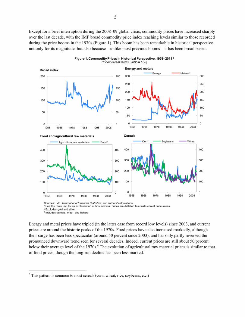
Except for a brief interruption during the 2008–09 global crisis, commodity prices have increased sharply over the last decade, with the IMF broad commodity price index reaching levels similar to those recorded during the price booms in the 1970s (Figure 1). This boom has been remarkable in historical perspective not only for its magnitude, but also because—unlike most previous booms—it has been broad based.
Energy and metal prices have tripled (in the latter case from record low levels) since 2003, and current prices are around the historic peaks of the 1970s. Food prices have also increased markedly, although their surge has been less spectacular (around 50 percent since 2003), and has only partly reversed the pronounced downward trend seen for several decades. Indeed, current prices are still about 50 percent below their average level of the 1970s.6 The evolution of agricultural raw material prices is similar to that of food prices, though the long-run decline has been less marked.
6 This pattern is common to most cereals (corn, wheat, rice, soybeans, etc.)
0
50
100
150
200
250
300
0
50
100
150
200
250
300
1958 1968 1978 1988 1998 2008
Energy Metals ²
0
100
200
300
400
0
100
200
300
400
1958 1968 1978 1988 1998 2008
Agricultural raw materials Food ³
Food and agricultural raw materials
0
50
100
150
200
0
50
100
150
200
1958 1968 1978 1988 1998 2008
Figure 1. Commodity Prices in Historical Perspective, 1958–2011 1(Index in real terms, 2005 = 100)
Sources: IMF, International Financial Statistics; and authors' calculations.1 See the main text for an explanantion of how nominal prices are deflated to construct real price series.2 Excludes gold and silver.3 Includes cereals, meat and fishery.
Broad index Energy and metals
0
100
200
300
400
0
100
200
300
400
1958 1968 1978 1988 1998 2008
Corn Soybeans Wheat
Cereals

6
Interestingly, food prices have also been less volatile and their shocks more persistent than those of metals and energy (Table 1)—although there are also marked differences within the food category, as prices for cereals tend to display relatively higher volatility and lower persistence than those of meat and fishery (to a large extent reflecting weather-related idiosyncratic shocks).
A look at the comovement across commodity prices suggests that the relationship between them has changed significantly over time, reflecting the varying nature of underlying shocks (Figure 2). Prices across all categories have tended to move in the same direction in the last decade, on account of the dominant role of global demand as a key common driver of price changes. They have also shown pronounced comovement in response to financial shocks, as seen during the 2008–09 crisis and, somewhat less markedly, in the second half of 2011. In previous decades, however—and particularly during past commodity boom-bust cycles—the correlation was lower, even negative in some cases. Clear examples are the first and second oil price shocks in the 1970s and the Gulf War shock in the early 1990s, in which the oil supply shocks triggered a slowdown in global economic activity, negatively affecting the demand for and price of other commodities (Figure A in Annex 1).
The importance of common (global) underlying factors in driving prices across different categories of commodities is confirmed by a statistical analysis of principal components (Table 2). In the last decade, the first principal component accounted for almost 85 percent of the variance of commodity prices, and prices of all categories were positively correlated with this underlying common force. This reflects to a great extent the increasing importance of China in global demand for commodities.7 In the 1970s and 1980s, in contrast, the first principal component accounted for about 65 percent of the variance of commodity prices, and whereas it was positively correlated with prices of metals and food, the correlation with energy prices was negative.
7 See the September 2006, April 2008, and October 2008 editions of the World Economic Outlook for more in-depth analyses of the underlying drivers of commodity prices in recent years.
0
10
20
30
40
0
10
20
30
40
Not statitiscally significant
Significant at the 10 percent level
Significant at the 1 percent level
1970s 1980s 1990s 2000s
Figure 2. Comovement across Commodity Prices¹(Groupwise correlation across categories, percent)
Sources: IMF, International Financial Statistics and authors' calculations.1 Based on monthly percentage changes of IMF commodity price indexes for energy, metals, and food, and on a statistic for a likelihood ratio test in which, under the null hypothesis, all pairwise correlations are equal to zero (i.e., the correlation matrix is equal to the identity matrix). See Valdes (1997) and Pindyck and Rotemberg (1990) for details.
Volatility
Autocorrelation HLS2 Std. dev. (dlog)
(24 months) (years) (percent)
Energy 0.70 9 8.2
Metals 0.70 9 3.9
Agricultural raw materials 0.26 2 3.0
Food 0.80 11 2.9
Cereals 3 0.58 4 5.8
1 Based on monthly data.
Table 1. Commodity Price Behavior, 1958–20111
Persistence
2 Half-life of a unit shock (HLS) is the length of time (in years) until the impulse response of a shock to prices is half its initial magnitude.3 Include corn, rice, soybeans, and wheat.
Sources: IMF, International Financial Statistics and authors' calculations.

7
Finally, despite their high correlation—especially recently—a glance at the behavior of commodity prices during global recessions suggests that there are notable differences across commodities in their sensitivity to the global cycle, with food prices being significantly less sensitive—possibly reflecting higher supply elasticity and lower income elasticity of demand (relative to other commodities). This lower impact was visible during the 2008–09 Great Recession as well as in other slowdowns in the last four decades (Figure 3).8 These differences across categories suggest that the degree of vulnerability to a global slowdown may vary significantly even within the group of commodity-exporting countries, depending on the specific commodities countries specialize in.
Consistent with global recessions being accompanied by lower commodity prices, net commodity exporters have been particularly affected during those episodes (Figure 4), displaying lower export (values and volumes) and domestic output growth than non-commodity exporters. Quantifying such impact, however, is challenging, as recent recessions have also been, in general, associated with tighter financing conditions for emerging markets (Figure 5), implying a “triple” shock—that is, weaker terms of trade, lower external demand, and tighter global financial conditions—for many commodity-exporting
8 A similar pattern was observed during the turbulence in global markets during the second half of 2011.
-12
-10
-8
-6
-4
-2
0
2
4
6
8
50
60
70
80
90
100
110
120
130
Energy prices Metal prices
Food prices Output gap (percent of potential, right scale)
Q2 Q3 Q4 Q1 Q2 Q3 Q4 Q12008 2009 2010
2008–09 Global Recession(Index, March 2008 = 100; and output gap in percent)
-2.5
-2.0
-1.5
-1.0
-0.5
0.0
0.5
1.0
1.5
2.0
70
75
80
85
90
95
100
105
110
t + 12 months
t + 24months
t
Previous Global Recessions, 1960–20082
(Index, t = 100; and output gap in percent)
Source: authors' calculations.1 Recessions defined on the basis of estimated output gap for advanced economies (using industrial production series). A slowdown is considered a recession if the output gap reaches at least –1. 5 percent of potential output for at least a quarter. Reported commodity prices are in real terms.2 t corresponds to the month of the peak value of the cyclical component of output, before ouput falls below potential. Only the first 30 months are reported as length of recessions varies across cases. Oil shocks of 1969 and 1973 are excluded.
Figure 3. Commodity Prices During Global Recessions, 1960–20101
1970s–80s 2000s
Share of variance explained by first principal component 0.63 0.84
Measure of comovement with
common global factor1
Food 0.63 0.56
Energy -0.36 0.59
Metals 0.68 0.58
Source: authors ' ca lculations .1 Loadings of fi rs t principa l component.
Table 2. Global Factors and Commodity Prices:
Principal Component Analysis

8
economies. This highlights the intrinsic difficulties of assessing the impact of price shocks, as many of these countries are hit by simultaneous and highly correlated shocks. In section IV we discuss the identification strategy to disentangle the effect of terms of trade shocks.
III. COMMODITY DEPENDENCE: LATIN AMERICA VS. EMERGING ASIA
The degree of a country’s reliance on commodity exports can be gauged with two different measures, that provide distict information:
A measure of commodity dependence, defined as total net exports of these basic products relative to the country’s GDP. This indicator provides information on the potential effect that a commodity price shock would have on domestic output.9
A measure of commodity export concentration, defined as gross commodity exports in percent of total exports of good and services. This second measure, that factors in the degree of a country’s trade openness, can inform about the country’s ability to adjust to a given commodity price shock. This potential source of strength has been pointed out by some authors (see, for instance, Calvo and Talvi, 2005), who have stressed the role of the relative size of the tradable sector (vis-à-vis the non-tradable sector) in determining the economy’s ability to adjust to an external shock.
9 Alternatively, one could focus on the size of the commodity sector in terms of their share of domestic output. Whether such measure would be preferable or not is not obvious, however, as our focus is on the income effect of changes in international prices. Such effect may net out in the case of commodities produced and consumed domestically.
-9
-7
-5
-3
-1
-9
-7
-5
-3
-1
Commodity exportersOthers
Peak TroughClosing
OG 2
Export prices
-10
-5
0
5
10
15
-10
-5
0
5
10
15
Peak TroughClosing
OG 2
Export volumes
0
2
4
6
8
10
0
2
4
6
8
10
Closing OG 2TroughPeak
Real GDP
Figure 4. Macro Performance of Commodity Exporters and Other Emerging Economies during Global Recessions, 1980–2010 1(Median cumulative growth, peak year = 0)
Source: authors' calculations.1 Median values are reported. Based on Hodrick-Prescott-filtered estimates of output gap for advanced economies, using industrial production. All recessions display the same pattern, except for the one following the 2008-09 financial crisis (the commodity price slump was short-lived in the latter case).2 Year at which estimated output gap closes.
Figure 5. Financial Conditions During Global Recessions, 1995–20101
10
12
14
16
18
20
22
24
26
28
30
200
300
400
500
600
700
800
900
1000
EMBIG spread (basis points)
VIX (right scale)
t + 12 months
t + 24months
t
Source: authors' calculations.1 Simple average. Recessions defined on the basis of output gap estimated from advanced markets' industrial production series. A slowdown is considered a recession if the estimated output gap reaches at least –1. 5 percent of potential output for at least a quarter. (t) corresponds to month of the peak value of the cyclical component of output, before output falls below potential. Only the first 30 months are reported as length of recessions varies across episodes.

9
In concrete, a larger tradable sector would entail a smaller real exchange rate depreciation in order to restore external sustainability in the event of a negative shock. In this vein, the higher vulnerability due to a growing share of commodity exports in GDP would be mitigated by an even more pronounced increase in exports of other goods.
Commodity Dependence
The degree of commodity dependence, as well as its evolution over time, differs significantly across emerging market regions (Figures 6 and 7, and Figures B, D, and F in Annex 1).
South America is the most commodity-dependent subregion, and this feature has become more pronounced over time (net commodity exports represented 10 percent of GDP in 2010, compared with 6 percent in 1970). Although the increase has been broad based, metals and energy still account for the largest shares of net commodity exports.
In contrast, Mexico and Central America have recorded sharp declines in net commodity exports, primarily as a result of falling agriculture exports and increasing energy imports. The subregion was a large commodity exporter in 1970 (8 percent of GDP) and currently shows balanced trade in commodities (still being a net exporter of agriculture goods but now also a net importer of energy).
The trends in emerging Asia greatly differ from those in Latin America, as the former has evolved from being a net commodity exporter (reaching around 6 percent of GDP in 1970) to being a net importer (almost 3 percent of GDP) in 2010. This shift has been mostly due to a sharp decline in exports of raw materials and an increase in imports of energy and metals. Most large emerging economies in Asia are now net importers of energy.
A comparison with some large commodity-exporting advanced economies (Australia, Canada, New Zealand, and Norway) also yields some interesting insights. As in the case of South America, dependence is high and has increased markedly in these advanced economies (from an average of 6 percent of GDP in 1970 to 13 percent in 2010).10
Commodity Export Concentration
While increasing dependence on commodities (as percent of GDP) has made some countries in South America more vulnerable to negative commodity price shocks, even larger increases in non-commodity exports (trade openess has grown markedly) have led in many cases to a more diversified export structure, arguably making these economies more flexible to withstand such shocks. Export diversification has been even more pronounced in Mexico and Central America, and—especially—in emerging Asia (Figures 6 and 7, and Figures C, E, and G in Annex 1):
10 Norway is the most commodity-dependent country in this group (net commodity exports represented 23 percent of GDP in 2010, with net oil exports accounting for 21 percent of GDP). Australia also recorded an increase in dependence, especially in the last decade, driven by the increasing importance of metals and—to a lesser extent—energy.
10
Several countries in South America (Argentina, Brazil, Uruguay) have diversified away from commodities, although the latter still account, on average, for 60 percent of total exports of goods and services. Interestingly, this diversification has not taken place in the case of the heavy metal or energy exporters. Indeed, metal (Chile and Peru) and energy exporters (Colombia, Ecuador, and Venezuela) still have higher concentrations of their exports, with metals (energy) accounting, on average, for about 60 percent (80 percent) of total exports. Moreover, these countries exhibit a higher degree of commodity dependence, with commodity exports averaging 20 and 17 percent of GDP, respectively, compared to only 8 percent in other countries in the region.11
In Mexico and Central America, the importance of commodity exports has also halved (from 50 percent of total exports to around 25 percent) between 1970–80 and 2010.12
Diversification in emerging Asia has been even starker, with commodity exports falling from about 60 percent of total exports in the 1970s to less than 20 percent in 2010.
Commodity-exporting advanced economies, in turn, have a less diversified export structure than 40 years ago. In fact, after declining slightly for three decades, the share of commodity exports in total exports increased sharply in the last decade for this group of countries, reaching—on average—60 percent in 2010. Interestingly, these countries appear to be more reliant on commodities—based on our dimensions of dependence and export concentration—than the emerging market regions in our sample.
Finally, the changing dependence on commodities in many countries has also been, at least partly, driven by growing commodity imports—reflecting primarily the increasing need for energy in rapidly expanding emerging market economies (Figure 6).
The share of commodities in Latin America’s total imports has increased markedly as a percentage of GDP (although not in terms of total imports) with energy remaining the main category of commodity imports across the region.
11 Two cases in this group show particularly interesting shifts: Colombia has exhibited a marked shift in its trade structure over the last four decades, even though the overall share of commodities has remained quite stable. Agricultural exports—which accounted for more than half of total exports in 1970–80—represent less than 10 percent today. In contrast, the share of energy exports has increased from less than 5 percent to 50 percent over the same period. As a percentage of GDP, net agricultural exports declined from about 5 percent to close to balance, whereas net energy exports surged from around zero to 8 percent over the same period. Venezuela has recorded a substantial decline in net energy exports, from 30 percent of GDP in 1990 to about 15 percent in 2010. However, diversification has declined markedly in this country, with commodity exports rising from 75 percent of total exports in 1980 to about 90 percent in 2010.
12 Mexico recorded a substantial decline in net energy exports, declining from 4½ to 1½ percent of GDP between 1980 and 2010. At the same time, it diversified away from those, with such exports currently amounting only to 13 percent of total exports (compared with about 50 percent in 1980).

11
-4
-2
0
2
4
6
8
10
12
1970 1980 1990 2000 2010-4
-2
0
2
4
6
8
10
12
Agriculture and related products
Animals and related products
Metals
Energy
Other raw materials
Total
Sources: World Integrated Trade Solutions database; and authors' calculations.1 Simple average for Argentina, Brazil, Chile, Colombia, Ecuador, Peru, Uruguay, and Venezuela.2 Simple average for Mexico, Costa Rica, El Salvador, and Guatemala.3 Simple average for China, India, Indonesia, Korea, Malaysia, Philippines, and Thailand.
-4
-2
0
2
4
6
8
10
12
1970 1980 1990 2000 2010-4
-2
0
2
4
6
8
10
12
-4
-2
0
2
4
6
8
10
12
1970 1980 1990 2000 2010-4
-2
0
2
4
6
8
10
12
Net commodity exports (Percent of GDP)
Figure 6. Commodity Dependence: A Regional and Historical Comparison
0
5
10
15
0
20
40
60
80
1970 1980 1990 2000 2010
Agriculture and related products
Animals and related products
Metals
Energy
Other raw materials
Total (percent of GDP, right scale)
South America1
Gross exports(Percent of total exports of goods and services, unless otherwise indicated)
0
5
10
15
0
20
40
60
80
1970 1980 1990 2000 2010
Mexico and Central America2
0
3
6
9
12
15
0
20
40
60
80
1970 1980 1990 2000 2010
Asia3
0
2
4
6
8
10
12
0
10
20
30
40
1970 1980 1990 2000 2010
Agriculture and related products
Animals and related products
Metals
Energy
Other raw materials
Total (percent of GDP, right scale)
0
2
4
6
8
10
12
0
10
20
30
40
1970 1980 1990 2000 2010
0
2
4
6
8
10
12
0
10
20
30
40
1970 1980 1990 2000 2010
Gross imports (Percent of total imports of goods and services, unless otherwise indicated)

12
Emerging Asia has shown a similar pattern, with the exception of China—where commodity imports have increased both as a fraction of total imports and as a percentage of GDP.
In sum, Latin America remains—on average—as exposed to commodities-related risk as four decades ago, making it vulnerable to a sharp decline in commodity prices. At the same time, higher export diversification (as non-commodity exports have grown even faster) has arguably made many of the countries in this region more flexible to withstand such shocks. This is not the case, though, for energy and metal exporters in the region, which are today particularly vulnerable to a global slowdown, given their higher overall commodity dependence and their greater concentration in commodities—heightened by their exposure to commodities that are more sensitive to the global economic cycle. In contrast,
Figure 7. Commodity Dependence and Export Concentration, 2010
Dependence (Net commodity exports in percent of GDP)
Export Concentration(Gross commodity exports in percent of total exports)
Sources: World Integrated Trade Solutions database and authors' calculations.

13
emerging Asia has evolved from being a strong net commodity exporter in 1970 to being a net importer in 2010, while also recording a marked export diversification, turning the region less vulnerable to a negative commodity price shock (from the perspective of a pure price shock).
A country’s ultimate degree of vulnerability is, however, also determined by the flexibility and quality of their policy frameworks. The role of policies in shaping the impact of shocks is examined in the next section.
IV. WHAT EXPLAINS ECONOMIC PERFORMANCE IN THE FACE OF TERMS OF TRADE BUSTS?
Although high commodity dependence can make emerging market countries vulnerable to a sharp turnaround in commodity prices, the potential economic impact of such a shock is not obvious. This is partly because the degree of commodity dependence can be mitigated by a diversified export structure (as discussed before) but also—and more importantly—because economic fundamentals and policies can play an important role in mitigating or amplifying the effects of price shocks.
Furthermore, the frequent concurrence of terms of trade and other external shocks (global growth or financial) makes it intrinsically difficult to observe the direct impact of price shocks, unless a multivariate setting is used (enabling the effect of different external factors to be disentangled from the price effect and its interactions with country economic fundamentals).
This section presents two complementary approaches for exploring the determinants of macroeconomic performance during episodes of sharp terms of trade drops—most of the time driven by commodity price shocks—in such a multivariate setting. The aim is to explain whether and to what extent country fundamentals and policies can shape the impact of these foreign shocks. The focus is on large terms of trade changes, as country fundamentals are likely to play a more important role when shocks are sizable (e.g., the flexibility of policy frameworks is more critical when the need for economic adjustment is large).
The first methodology entails a cross-sectional study of episodes of sharp negative terms of trade shocks that took place between 1970 and 2010 in a sample of 64 emerging and large commodity-exporting advanced economies. After documenting the behavior of key macroeconomic variables during these episodes, we explore the role of fundamentals in determining the overall impact of the external price shock on domestic output.
This approach is complemented by a similar exercise in a panel setting, which allows us to explore the importance of certain variables for which reliable data are available only for a shorter and more recent time span (e.g., degree of dollarization, fiscal stance).
Unlike other studies—which have focused mostly on the traditional measure of terms of trade (export prices over import prices)—we rely on an adjusted measure that captures the magnitude of the income effect of changes in trade prices, taking into account the initial export and import ratios to GDP (that is,

14
the direct impact of the changes in export and import deflators on the trade balance, given volumes).13 Specifically:
X M ;
where Xand Mdenote the percentage change in export and import deflators, respectively, and
and are the previous-year ratios of exports and imports to GDP.
A. Cross-Sectional Approach
The cross-sectional approach entails assessing whether country fundamentals at the outset of the shock can explain cross-country differences in macroeconomic performance during the full length (i.e., from peak to trough) of episodes of sharp and negative terms of trade shocks. Episodes are identified on the basis of whether a country experienced a cumulative drop in its (adjusted) terms of trade of at least 3 percentage points of GDP, from peak to trough (with negative changes in at least two consecutive years). The threshold is somewhat arbitrary. It is set at a relatively high level to increase the likelihood of identifying an economic impact and at the same time not too high in order to preserve a reasonable sample size. By requiring at least two consecutive years of terms of trade declines, our sample does not include any episode around the 2008–09 global crisis, given that the commodity price drop proved to be short-lived.
This criterion identifies 98 episodes (Figure 8). The sample of countries includes both commodity exporters and importers, in order to disentangle the price effect from the effect of other external shocks that could be highly correlated with commodity prices (e.g., global growth). Terms-of-trade shocks induced by export prices do not appear to have a different impact than those induced by import prices.
Interestingly, although there is a prevalence of episodes during the commodity shocks of the 1970s and 1980s, there are still a fair number of episodes dated in the last two decades—although the latter reflect primarily shocks to commodity-importing countries arising from higher import prices, rather than from lower export prices. In most cases, terms of trade shocks have been quite persistent, with an average peak-to-trough time span of 4½ years.
The magnitude of these shocks has been wide ranging, and so has output performance during the episodes—suggesting that, despite being sizable, the price shocks cannot by themselves explain the differences in macroeconomic performance (Figure 9). In fact, only two-thirds of the episodes show negative cumulative growth (relative to the preshock average), and the fraction falls to one-half for the subsample of episodes taking place during the 2000s. This reflects the importance of other external
13 This measure can be (loosely) interpreted as a combination of standard terms of trade and trade openness. It does not attempt to capture, however, the economy’s ability to adjust to an external price shock—as raised by Calvo and Talvi, 2003—but the net trade gains or losses (in terms of GDP) from shifts in export and import prices. Econometric results confirm that this measure of terms of trade is more informative than the traditional ratio of export to import prices, as the latter does not deliver statistically significant results.

15
factors in driving economic growth, as the latter period was characterized by favorable global growth and financial conditions.
Algeria 0 0 0 0 0 0 0 0 0 0 0 0 0 0 0 0 0 2 2 2 2 0 0 2 2 2 2 0 0 0 0 0 0 0 0 0 0 0 0 0 0
A rgentina 0 0 0 0 0 0 0 0 0 0 0 2 2 2 2 0 0 0 0 0 0 0 0 0 0 0 0 0 2 2 2 2 2 2 2 0 0 0 0 0 0
Australia 0 0 0 0 0 2 2 2 2 2 0 0 0 0 0 0 0 0 0 0 0 0 0 0 0 0 0 0 0 0 0 0 0 0 0 0 0 0 0 0 0
Bo livia 0 0 0 0 0 0 2 2 2 2 2 0 0 0 0 0 0 0 0 0 2 2 2 2 2 0 0 0 0 0 0 0 0 0 0 0 0 0 0 0 0
Chile 0 2 2 2 2 2 2 2 0 0 0 2 2 2 2 2 2 2 2 0 0 0 0 0 0 0 0 0 0 0 0 0 0 0 0 0 0 0 0 0 0
Co lombia 0 0 0 0 0 0 0 0 0 2 2 2 2 0 0 0 0 0 2 2 2 2 2 2 2 2 2 0 0 0 0 0 0 0 0 0 0 0 0 0 0
Costa Rica 0 0 1 1 1 1 1 0 0 2 2 2 2 2 2 0 0 0 2 2 2 2 2 2 2 0 0 0 2 2 2 2 2 2 1 1 1 1 1 1
Dominican Rep. 0 0 0 0 0 0 0 2 2 2 2 2 0 0 0 0 0 0 0 0 1 1 1 1 1 1 0 0 0 0 0 0 0 0 0 0 0 1 1 1 1
Ecuador 0 0 0 0 0 0 0 0 0 0 0 0 2 2 2 2 2 2 2 2 2 0 0 2 2 2 2 2 2 2 2 0 0 0 0 0 0 0 0 0 0
Egypt 0 0 0 0 0 0 0 0 0 0 0 0 0 2 2 2 2 0 0 0 0 0 0 0 0 0 0 0 0 0 0 0 0 0 1 1 1 0 0 0 0
El Salvador 0 0 0 0 0 0 0 0 0 0 0 0 0 0 0 0 0 0 0 0 0 0 0 0 0 0 0 0 0 2 2 2 2 2 2 2 2 2 2 2 2
Guatemala 0 0 0 0 0 0 0 0 0 2 2 2 2 2 2 0 0 0 0 0 0 0 0 0 0 0 0 0 0 2 2 2 2 2 2 2 2 2 2 2 2
Hungary 2 2 2 2 2 2 2 2 2 2 0 0 0 0 2 2 2 2 2 0 0 0 0 2 2 2 0 0 0 0 0 0 0 0 0 0 2 2 2 0 0
Iceland 0 0 0 0 0 0 0 0 0 0 2 2 2 2 2 2 2 0 0 2 2 2 0 0 0 0 0 0 0 0 0 0 0 0 0 0 0 0 1 1 1
India 0 0 0 0 0 0 0 0 0 0 0 0 0 0 0 0 0 0 0 0 0 0 0 0 0 0 0 0 0 0 0 0 0 0 1 1 1 1 1 1 1
Indonesia 0 0 0 0 0 0 0 0 0 0 0 0 0 0 0 0 0 2 2 2 2 0 0 0 0 0 0 2 2 2 2 0 0 0 0 0 0 0 0 0 0
Israel 0 1 1 1 1 1 1 0 0 0 0 0 0 0 0 0 0 0 0 0 0 0 0 0 0 0 0 0 0 0 0 2 2 2 2 2 2 2 2 2 0
Jamaica 0 0 0 0 1 1 1 0 0 0 0 0 0 0 1 1 1 1 0 0 2 2 2 2 2 2 0 0 0 0 2 2 2 2 2 2 2 2 2 2 2
Jordan 0 0 0 0 0 0 0 0 0 0 0 0 0 0 0 0 0 0 0 0 0 0 0 0 0 0 0 0 2 2 2 2 2 2 2 2 2 0 0 0 0
Korea 0 0 0 1 1 1 1 0 0 0 2 2 2 0 0 0 0 0 0 0 0 0 0 0 0 0 2 2 2 2 2 2 2 2 0 0 1 1 1 1 1
Libya 0 0 0 0 0 0 2 2 2 2 2 0 0 0 0 0 0 2 2 0 0 0 0 0 0 0 0 0 0 0 0 0 2 2 2 0 0 0 0 0 0
M alaysia 0 1 1 1 1 1 1 1 0 0 0 2 2 2 2 0 0 0 0 0 0 0 0 0 0 0 0 0 0 0 0 2 2 2 0 0 0 0 0 0 0
M exico 0 0 0 0 0 0 0 0 0 0 0 2 2 2 2 2 2 2 0 0 0 0 2 2 2 0 0 2 2 2 2 2 2 2 0 0 0 0 0 0 0
M orocco 0 0 0 0 0 0 0 0 0 0 0 0 0 0 2 2 2 2 2 2 2 2 0 0 0 0 0 0 0 0 0 0 0 0 0 0 0 0 0 0 0
New Zealand 0 0 0 0 0 2 2 2 0 0 0 0 0 0 0 0 0 0 0 0 0 0 0 0 0 0 0 0 0 0 0 0 0 0 0 0 0 0 0 0 0
Nigeria 0 0 0 0 0 0 0 0 0 0 0 0 0 0 0 0 2 2 2 0 0 0 2 2 2 2 2 2 0 0 0 0 0 0 0 0 0 0 0 0 0
Norway 0 0 0 0 0 1 1 1 1 1 0 0 0 0 0 0 2 2 2 2 2 0 0 0 0 0 0 0 0 0 0 0 0 0 0 0 0 0 0 0 0
Pakistan 0 0 0 0 0 2 2 2 0 0 0 2 2 2 0 0 0 2 2 2 0 0 0 0 0 0 0 0 0 0 0 0 0 0 1 1 1 1 0 0 0
Panama 0 1 1 1 1 1 1 1 1 1 1 1 0 0 0 0 0 0 0 0 2 2 2 2 2 0 0 0 0 0 0 0 0 0 0 0 0 0 0 0 0
Paraguay 0 0 0 0 0 0 0 0 0 2 2 2 0 0 0 0 0 0 0 0 0 0 2 2 2 2 0 0 0 2 2 2 2 0 0 0 2 2 2 0 0
Peru 0 0 0 0 0 2 2 2 2 2 2 0 0 0 0 0 2 2 2 0 0 0 0 0 0 0 0 2 2 2 2 2 2 2 0 0 0 0 0 0 0
Philippines 0 0 0 0 0 0 2 2 2 2 0 0 0 0 0 0 0 0 0 0 0 0 0 1 1 1 1 1 1 1 1 1 1 0 0 0 0 0 0 0 0
Po land 0 0 0 0 0 2 2 2 2 2 2 2 2 2 2 2 2 0 0 0 0 0 0 0 0 0 0 0 0 0 0 0 0 0 0 0 0 0 0 0 0
Qatar 0 0 0 0 0 0 0 0 0 0 0 0 0 2 2 2 2 2 2 0 0 2 2 2 2 2 2 0 0 0 0 0 0 0 0 0 0 0 0 0 0
Saudi Arabia 0 0 0 0 0 0 0 0 0 0 0 0 0 0 0 0 0 0 0 0 0 0 2 2 2 2 2 0 0 0 0 0 0 0 0 0 0 0 0 0 0
South Africa 0 0 0 0 0 1 1 1 1 1 1 1 0 0 0 0 0 0 0 0 0 0 0 0 0 0 0 0 0 0 0 0 0 0 0 0 0 0 0 0 0
Sri Lanka 1 1 1 1 1 1 1 0 0 2 2 2 2 2 2 0 0 0 0 0 0 0 0 0 0 0 0 0 0 0 0 0 0 0 0 2 2 2 2 2 2
Thailand 0 0 0 0 0 0 0 0 0 2 2 2 2 2 2 0 0 0 0 0 0 0 0 0 0 0 0 0 2 2 2 2 2 2 0 0 0 0 0 0 0
Tunisia 0 0 0 0 0 0 0 0 0 0 0 0 0 0 2 2 2 2 2 0 0 0 0 0 0 1 1 1 1 0 0 0 0 0 1 1 1 1 1 1 0
Turkey 0 0 0 0 0 0 0 0 0 1 1 1 1 0 0 0 0 0 0 0 2 2 2 0 0 0 0 0 0 0 0 0 0 0 1 1 1 1 1 1 1
United Arab Em. 0 0 0 0 0 0 0 0 0 0 0 0 0 0 0 0 0 0 0 0 0 0 2 2 2 2 2 0 0 0 0 0 0 0 0 0 0 0 0 0 0
Uruguay 0 0 0 0 0 2 2 2 0 0 2 2 2 2 2 2 2 2 0 0 0 0 0 0 0 0 0 0 0 0 0 0 0 0 0 0 0 0 0 0 0
Venezuela 0 0 0 0 0 0 0 0 2 2 2 0 0 2 2 2 2 2 2 0 0 0 2 2 2 2 2 2 2 2 2 0 0 0 0 0 0 0 0 0 0
Number of episodes 2 6 7 8 9 17 20 16 12 19 18 19 16 16 19 13 16 17 16 9 13 10 14 17 17 14 11 9 12 14 15 14 15 13 13 12 15 14 14 12 10
Figure 8. Episodes of Terms of Trade Busts¹(Time span of each episode)
26 7 8 9
1720
1612
19 18 1916 16
19
1316 17 16
913
1014
17 1714
11 912 14 15 14 15 13 13 12
15 14 14 12 10
0
10
20
Source: authors' calculations.¹ Episodes of negative (adjusted) terms of trade shocks of at least 3 percentage points of GDP, cumulative peak to trough. Lighter blue shading corresponds to episodes in which the terms of trade drop is not accompanied by a drop in real (U.S. CPI-deflated) export prices (i.e., the change in terms of trade comes from import prices).

16
A breakdown by region indicates that, for shocks of similar magnitude, Latin America appears to have been more affected than other regions (Figure 10). Since our measure of terms of trade already factors in the countries’ degree of trade openness, this disparity in economic impact suggests that other economic fundamentals may have played a role in amplifying the impact of these shocks.
A glance at the dynamics of key macro variables around the episodes, comparing best and worst macro performers (in terms of GDP growth) offers some additional insights (Figure 11):
There is considerable difference between the best and the worst performers, with evidence suggesting that those growing faster before the shock (while external conditions were favorable) suffer the most with the reversal.
Interestingly, these two groups do not appear to have faced significantly different trade prices, either during the boom or the subsequent bust.
-50 -40 -30 -20 -10 0-50
-40
-30
-20
-10
0
10
20
30
40
50
-50
-40
-30
-20
-10
0
10
20
30
40
50
Rea
l GD
P g
row
th¹
Terms of trade shock²
Figure 9. Terms of Trade Shocks and GDP Growth(Cumulative, peak to trough)
Source: authors' calculations.¹ Cumulative difference with respect to prebust (t–3 to t) growth. tis the last year before the drop in terms of trade.² Cumulative direct effect in adjusted terms of trade, in percent of GDP.
Source: authors' calculations.¹ Cumulative difference with respect to prebust (t–3 to t–1) growth, in percentage points.² Cumulative direct effect in adjusted terms of trade, in percent of GDP.
Emerging LA Emerging Asia Other Emerging Markets
-14
-12
-10
-8
-6
-4
-2
0
-6
-5
-4
-3
-2
-1
0
Real GDP growth¹
Terms-of-trade shock (right scale)²
Figure 10. Performance by Region(Percent, simple averages)
0
1
2
3
4
5
6
7
0
1
2
3
4
5
6
7
t–3 t–1 t+1 t+3 t+5
Best performers' averageBest performers' medianWorst performers' averageWorst performers' median
Growth (Percent)
Terms of trade (adjusted)(Percent of GDP, cumulative t-3=0)
Underlying Current Account (Percent of GDP)
Current Account (Percent of GDP)
Figure 11. Key Fundamentals of Best and Worst Performers in Terms-of-Trade Busts ¹(Centered at terms-of-trade peak year, t)
Sources: IMF International Financial Statistics, and authors' calculations. ¹ Statistics of upper and lower halves of the sample of episodes, ranked on the basis of the average GDP growth in [t+1,t+3] relative to the preepisode [t–3,t–1] average.
t–3 t–1 t+1 t+3 t+5-6
-4
-2
0
2
4
6
8
-6
-4
-2
0
2
4
6
8
t–3 t–1 t+1 t+3 t+5-6
-5
-4
-3
-2
-1
0
1
-6
-5
-4
-3
-2
-1
0
1
t–3 t–1 t+1 t+3 t+5-9-8-7-6-5-4-3-2-101
-10
-8
-6
-4
-2
0
2

17
As most episodes of price busts were preceded by improving terms of trade, current account balances often strengthened before the negative shock.
However, underlying current accounts (stripped of terms of trade changes) weakened markedly.
Overall, macro performance during these episodes appears to reflect more than simply the effect of the terms of trade, to the extent that countries facing more favorable price dynamics do not appear to have outperformed the rest (Annex 2). These stylized facts reinforce the need for a multivariate setting in order to properly examine the determinants of output performance in the face of large terms of trade shocks.
With this aim, we first estimate a simple regression model to identify the effects of fundamentals on output performance during the episodes, controlling for the size of the shock and other external factors. The specification is as follows:
α β A β′ β′ ε
Where:
Yi is the output performance in episode i, (measured as the cumulative difference between annual growth during the episode and the average growth rate in the preshock period). The average growth rate is computed over the five-year period up to the shock. We also use the three-year period preceding the shock and the main results do not change significantly.
ToTiA is the (adjusted) terms of trade cumulative change during episode i;,
Xi is a vector of variables reflecting fundamentals and policies in the run-up to the shock, and
Zi is a vector of controls (external factors).
We focus on the following explanatory variables that—to different degrees—reflect economic policies:14
The external position, as reflected by the current account, external debt or international reserves (either the level at the time of the shock or the change in the three years preceding the episode).
A measure of “de facto” exchange rate flexibility, using the classification of Ilzetzki, Reinhart, and Rogoff (2008).15
The occurrence of a credit boom during the three-year period preceding the shock, as identified by either Gourinchas, Landerretche, and Valdes (2001) or Mendoza and Terrones (2008).
14 All explanatory as well as control variables are explained in detail in Annex 3.
15 We also explore an alternative measure based on the standard deviation of the monthly percentage changes of the nominal exchange rate (over a 12-month window).

18
We also explore the role of financial openness—which could determine the country’s ability to obtain foreign funding to buffer the shock—using a measure of capital account openness based on the index constructed by Chinn and Ito (2008), as well as a measure of international financial integration, calculated as the sum of the countries’ total foreign assets and liabilities—in percent of GDP—from the updated and extended version of the Lane and Milesi-Ferretti (2007) data set. The use of two different measures of financial openness allows us to properly interpret the results of the regression, as discussed below.
While we include public debt in the set of explanatory variables, other fiscal and financial sector variables are not included in this approach.16 In particular, we do not include in the cross-section analysis any measure of the fiscal stance or the cyclical behavior of fiscal policy in the period preceding the episode. This reflects poor data quality and/or coverage for a number of episodes that date back to the 1970s and 1980s. In the case of financial variables (notably, financial dollarization), it is because insufficient variance across episodes in those decades also precludes proper econometric examination. These variables, however, are explored in the panel approach presented in the next section.
External factors used as controls are global demand (proxied by world real GDP growth) and global financial conditions (using the Chicago Board Options Exchange Market Volatility Index, VIX, and the 10-year U.S. Treasury Bond yield).
Following a “specific-to-general” approach, we first regress output performance on each of the fundamentals, controlling for the size of the shock and for external conditions. Then, we include all the relevant fundamentals (and control variables) in a single regression. A negative value in our dependent variable indicates a loss of output, therefore a positive (negative) coefficient on an explanatory variable implies that this variable mitigates (exacerbates) the negative impact of the terms of trade shock on output.
Regressions are estimated using ordinary least squares with robust standard errors. For the sake of brevity, in Table 3 we omit the coefficients of the external controls. Results may underestimate the effect of terms-of-trade shocks to the extent that some price movements arise from idiosyncratic shocks in countries with a large share in global supply of commodities (e.g., an unexpected increase in production of copper in Chile leading to a fall in international copper prices and, thus, on Chile’s terms of trade).
The main results are as follows (Figure 12 and Table 3):
The output loss is smaller in countries with a stronger external position, as reflected in any of the current account measures (columns 1–2 and 6–9 in the table). The result holds when the change in terms of trade in the three years preceding the shock is controlled for, suggesting that countries with a weaker (or deteriorating) underlying current account position tend to underperform in the aftermath of large terms of trade declines.
16 We consider public debt in percent of GDP, both the level at the time of the shock and the change in the three years preceding the episode.

19
Moreover, the negative impact of a weak external position is larger, the larger the preceding terms of trade boom (columns 10–11).
There is robust evidence that the decline in output is smaller in countries with more flexible exchange rate regimes (see columns 3–4 and 6–11), supporting the notion that exchange rate flexibility significantly enhances the economy’s ability to adjust to real external disturbances.
We find no evidence that countries’ external (or public) debt position explains differences in output performance during the bust. This may reflect the fact that countries with stronger policies typically have greater access to markets and can afford higher debt ratios without raising concerns about debt sustainability. Similarly, neither international reserves nor credit booms appear to have played a role. The muted result in regard to international reserves could reflect the fact that monetary authorities are often reluctant to make use of their reserve holdings to mitigate negative external shocks. This appears to have been the case, for instance, during the 2008 global financial crisis, when even countries with large amounts of reserves did not run down their holdings significantly.
A higher degree of capital account openness appears to be associated with larger output costs (columns 5–10), suggesting that capital inflows have, at least on average, been procyclical in the cases examined. However, the degree of capital procyclicality is likely to depend on the quality of country fundamentals. This caveat is particularly important in regard to our study, since many of the identified episodes from the 1970s and 1980s featured relatively weak policy frameworks. In fact, there is a vast literature pointing to the counterproductive effects of premature capital account liberalizations in developing countries. In fact, when using the measure of international financial integration, the result reverts. This is because the latter better captures the interaction of financial openess and quality of fundamentals (as countries with good fundamentals tend to be more financially integrated). These results suggest that financial openness helps buffer the shock when country fundamentals are strong but could exacerbate it when fundamentals are weak.
Finally, there is strong evidence that other external factors (notably, international interest rates and the degree of risk aversion, as reflected in the VIX) are also significant determinants of output performance during the bust.
0.0
0.5
1.0
1.5
ToT boom No boom
Benefit of a 1-percent-of-GDP higher current account balance
0
5
10
15
ToT boom No boom
Benefit of a flexible exchange rate regime
Sources: IMF, International Financial Statistics; and authors' calculations.1 Impact on cumulative output growth during the episode, as defined in the text. Based on column 10 of Table 3.3. ToT boomreflects the increase in the adjusted terms of trade (prior to the bust) of the 75th percentile of the sample (around 6 percent). No boom reflects the increase of the 25th percentile of the sample (roughly zero).
Figure 12. Policies and Output Performance: Does It Matter if the Bust was Preceded by a Boom?(Percentage points of GDP growth)1

20
(1) (2) (3) (4) (5) (6) (7) (8) (9) (10) (11)
ToT A 2 0.264 0.284* 0.205 -0.113 0.160 0.092 0.012 0.159 0.020 0.135 0.096(0.23) (0.17) (0.20) (0.19) (0.15) (0.26) (0.27) (0.23) (0.22) (0.199) (0.200)
CA (percent of GDP, level in t ) 3 0.568* 0.615+ 0.648* -0.105 -0.101(0.29) (0.42) (0.37) (0.37) (0.36)
CA_2 (percent of GDP, change t -3, t ) 3 0.503** 0.557* 0.456**(0.20) (0.30) (0.23)
ER Regime 4 -10.59** -9.084* -10.50** -9.589* -13.54***(4.43) (4.57) (4.74) (4.80) (4.59)
FXVol 5 0.946*** 0.707** 0.701**(0.32) (0.34) (0.32)
KA openness 6 -2.030* -1.755 -2.036 -1.567 -1.991 -2.339+
(1.21) (1.50) (1.50) (1.58) (1.45) (1.45)
Fin. Integ. 7 0.071***(0.02)
CA x ToT A Prev 8 0.222*** 0.133**(0.08) (0.06)
ER Regime x ToT A Prev 8 -0.277 -0.209(0.51) (0.48)
ToT A Prev 8 0.129 0.191(0.48) (0.44)
Constant -1.27 -3.43 0.62 -7.70** -3.86 -0.29 -5.68** -1.35 -7.57*** -0.86 -6.60(2.75) (2.34) (2.70) (2.97) (2.40) (3.19) (2.83) (2.67) (2.78) (3.25) (4.36)
Number of observations 91 93 79 68 92 70 64 73 66 70 70R ² 0.103 0.114 0.131 0.119 0.102 0.207 0.213 0.211 0.206 0.305 0.332
Source: authors' calculations.
2 Cumulative change in the adjusted terms of trade measure, from peak to trough.3 Current account balance, percent of GDP, in period t or change from t –3 to t, as indicated.4 Exchange rate flexibility, based on Ilzetzki, Reinhart, and Rogoff (2008) de facto index, at t . Dummy = 1 if index is between 1 and 4 (fixed), 0 if between 4 and 13 (flexible).5 Standard deviation of the monthly percentage changes of the nominal exchange rate (over a 12-month window).6 Chinn and Ito (2008) capital account openness index, average t –2 to t.7 Measure of financial integration, defined as the sum of total external assets and total external liabilities (in percent of GDP).8 Cumulative change in the adjusted terms of trade measure, in the three-year period before the shock.*** p<0.01, ** p<0.05, * p<0.1, + p<0.15.
Table 3. Cross-Sectional Approach: Results1
Dependent variable: Cumulative output growth during the bust (Yi), relative to trend growth
1 Regressions estimated using ordinary least squares with robust standard errors (in parentheses). Regressions include controls for global factors (coefficients not shown).

21
B. Panel Approach
A large number of the episodes identified under the previous methodology date back to the 1970s and 1980s. As mentioned previously, this poses a constraint on our ability to assess the importance of some fiscal and financial sector features, in the first case because of unavailable or unreliable data, and in the second case because of insufficient variance across countries and time for those decades. An example of the latter is financial dollarization, a feature that arose widely only during the 1980s, partly as a result of the move towards capital account liberalization. Hence, we complement the cross-sectional exercise with a panel approach that allows us to exploit the time series dimension of fiscal and financial variables, for which recent data are more reliable and show higher variation.
Our interest here is in assessing the potential “amplifying” role of certain fundamentals in regard to the impact of large and negative terms-of-trade shocks. We estimate the following specification in a panel setting with fixed effects:
, β β ,A β′ ,
′, , ε ,
where:
, is country i’s real GDP growth at year t,
,A is the adjusted measure of terms of trade;
, is a vector of exogenous control variables (including world real GDP growth, the U.S. 10-
year Treasury Bond yield, and the VIX);
, is a variable that takes the value of the terms of trade shock at year t ( ,A ) if the latter is
lower than a certain threshold (set at -1.5 percentage points of GDP in our benchmark estimation). This threshold implies that about 20 percent of the annual observations are considered large and negative shocks; and
, is a vector of country i’s economic fundamentals that (have the potential to) amplify the
impact of terms of trade shocks.
Our interest is in the vector of coefficients β as it provides insights on which and to what extent certain
economic fundamentals can exacerbate the effect of such shocks, over and above their direct effect. Under this specification the direct marginal effect of a large and negative terms of trade shock can be
computed as (β β′ FEM) where FEM is the vector of fundamentals evaluated at the average value for the
sample of countries. The amplification effect of country i’s policies (relative to an average country), on
the other hand, can be calculated as β′ F , FEM ). Results are robust to an alternative specification that
incorporates the level of policy variables, in addition to their interactions with I , . Results also hold if the dependent variable is measured relative to potential growth (with the latter proxied by the 10-year moving average).

22
The following set of macroeconomic fundamentals is explored:
Public and external debt, current account, and net foreign assets (in percent of GDP).
A measure of “de facto” exchange rate flexibility, as discussed in the previous section.
A measure of financial dollarization, defined as the share of foreign currency deposits in total deposits of the banking system. We rely on Levy Yeyati’s database, although we augment it (using information from multiple sources, including IMF staff reports, academic papers, and country documents) to extend the series back to the 1970s for a number of countries.
The primary fiscal balance, in percent of GDP, as a measure of the fiscal position.
A measure of capital account openness, based on Chinn and Ito’s (2008) index, normalized to range from 0 to 1, with 1 being the most open.
The measure of international financial integration described previously.
We estimate two alternative specifications of the model. The first examines the role of policies in amplifying or mitigating the impact of all large and negative shocks (of at least 1½ percent of GDP). The second one examines the particular case of large negative shocks (also of at least 1½ percent of GDP) that were preceded by improving terms of trade (in the three previous years).17 This second specification allows us to explore specifically to what extent policy responses during the boom phase of commodity price ‘boom-bust cycles’ determine the impact of subsequent large price reversals.
Results unveil a number of insights (Table 4):
While terms of trade appear to explain relatively little of the variance in growth (see R2 in column 1), the estimation captures an unambiguous and statistically significant effect: a negative terms-of-trade shock of 1 percentage point of GDP would lead to 0.13 percent lower growth in the same year of the shock and 0.08 percent lower growth in the second year. The introduction of the external variables as controls reduces only marginally the coefficients of terms of trade, suggesting that the correlation between these other factors and terms of trade is relatively low in the sample. To a great extent this reflects the fact that the sample includes both commodity exporters and importers. Any correlation between global financial and growth variables and commodity prices tends to disappear when the full sample is used (unlike the case of the subsample of commodity exporters). This highlights the advantage of including commodity importers, to better disentangle the price effect from the impact of other global shocks.
17 In the first case the variable , takes the value of the terms-of-trade shock if the latter is lower than -1.5 percentage points of GDP. In the second case, , takes the value of the terms-of-trade shock if the latter is lower than -1.5 percentage points of GDP and the previous three years were characterized by positive terms of trade shocks.

23
Sample period: 1970–2007 Base
With ext. controls
Variable (1) (2) (3) (4) (5) (6) (7) (8) (9) (10) (11) (12) (13) (15) (16) (17) (18) (19)
Terms of trade 2 0.131*** 0.100*** 0.077* 0.070 0.093+ 0.070* 0.081** 0.084* -0.023 0.069* 0.074* 0.061 0.024 0.090** 0.090** 0.004 0.002 0.002(0.037) (0.035) (0.045) (0.049) (0.058) (0.036) (0.035) (0.047) (0.072) (0.037) (0.040) (0.043) (0.053) (0.035) (0.034) (0.054) (0.055) (0.055)
Lagged terms of trade 2 0.082** 0.074** 0.070 0.122*** 0.115*** 0.068+ 0.078** 0.080** 0.032 0.072 0.136*** 0.119** 0.092** 0.087** 0.091** 0.033 0.031 0.032
(0.036) (0.036) (0.053) (0.032) (0.042) (0.041) (0.037) (0.039) (0.055) (0.052) (0.034) (0.045) (0.038) (0.036) (0.034) (0.055) (0.056) (0.056)Lagged real GDP (level) -0.002 -0.009 -0.000 -0.009 0.025*** 0.002 -0.002 0.026** -0.009 0.000 -0.010 0.025*** 0.002 -0.002 0.025** 0.025** 0.025**
(0.008) (0.008) (0.010) (0.010) (0.009) (0.008) (0.008) (0.011) (0.008) (0.010) (0.010) (0.009) (0.008) (0.008) (0.011) (0.011) (0.011)
World GDP growth 0.477*** 0.462*** 0.419*** 0.407*** 0.516*** 0.439*** 0.495*** 0.452*** 0.458*** 0.393*** 0.403*** 0.513*** 0.422*** 0.486*** 0.405*** 0.401** 0.402**(0.091) (0.090) (0.090) (0.090) (0.140) (0.087) (0.085) (0.149) (0.092) (0.083) (0.090) (0.139) (0.088) (0.087) (0.149) (0.150) (0.150)
U.S. 10-year Treasury Bond Yield -0.296*** -0.231*** -0.268*** -0.266*** -0.071 -0.288*** -0.297*** -0.035 -0.231***-0.250***-0.264*** -0.093 -0.278***-0.294*** -0.042 -0.042 -0.043
(0.069) (0.066) (0.081) (0.080) (0.086) (0.069) (0.071) (0.064) (0.065) (0.079) (0.078) (0.080) (0.069) (0.071) (0.064) (0.064) (0.064)VIX -0.107*** -0.110*** -0.098*** -0.119*** -0.096*** -0.113*** -0.108*** -0.107*** -0.111***-0.101***-0.119***-0.099***-0.116***-0.111***-0.109***-0.110***-0.110***
(0.021) (0.023) (0.023) (0.023) (0.023) (0.021) (0.020) (0.030) (0.024) (0.022) (0.023) (0.024) (0.021) (0.021) (0.029) (0.030) (0.030)
ER flexibility (t–1) 4 -0.001 -0.015 0.053* 0.019 -0.042 -0.239*** -0.043 -0.181***
(0.013) (0.011) (0.030) (0.037) (0.036) (0.025) (0.086) (0.027)Dollarization (t–1) 5 0.004 0.050***
(0.004) (0.018)ER flexibility * Dollarization (t–1) 6 0.000 -0.000 0.007 0.006*** 0.005*** 0.006***
(0.000) (0.000) (0.005) (0.001) (0.001) (0.000)Primary fiscal balance (t–1) 7 -0.038*** -0.023*** -0.096*** -0.428***-0.428***-0.429***
(0.013) (0.008) (0.021) (0.020) (0.035) (0.014)
Capital account openness 8 0.103 0.251 0.802*** 2.437*** 2.202***(0.121) (0.258) (0.270) (0.320) (0.255)
Financial integration 9 0.059 -0.456+ 0.390* -1.573** -0.491
(0.099) (0.281) (0.217) (0.599) (0.342)Constant 4.256*** 6.332*** 6.698*** 6.191*** 7.319*** 2.470** 6.293*** 6.335*** 2.768** 6.744*** 6.166*** 7.408*** 2.744*** 6.288*** 6.342*** 3.109** 3.119** 3.122**
(0.009) (0.852) (0.865) (1.038) (1.062) (1.022) (0.861) (0.866) (1.194) (0.902) (1.020) (1.066) (0.979) (0.849) (0.894) (1.163) (1.165) (1.165)
Number of observations 2,025 2,025 1,567 1,571 1,227 1,130 1,970 1,879 760 1,567 1,571 1,227 1,130 1,970 1,879 767 760 760R ²- within 0.023 0.089 0.090 0.084 0.109 0.125 0.091 0.098 0.100 0.090 0.102 0.110 0.128 0.097 0.103 0.100 0.100 0.101R ²- between 0.006 0.004 0.154 0.008 0.133 0.039 0.003 0.004 0.261 0.164 0.055 0.172 0.006 0.001 0.002 0.234 0.236 0.242R ²- overall 0.015 0.077 0.088 0.070 0.105 0.069 0.075 0.085 0.029 0.089 0.089 0.109 0.081 0.080 0.088 0.035 0.035 0.035
Number of countries 64 64 59 61 55 57 63 63 49 59 61 55 57 63 63 50 49 49
Source: authors' calculations.
8 Index of Chinn and Ito (2008) normalized to range between 0 and 1 (1 being the most open).9 Total foreign assets plus total foreign liabilities, in percent of GDP. Countries with the U.S. level or higher are classified as fully integrated. For other countries, the measure is reported relative to the level of the U.S.*** p < 0.01, ** p < 0.05, * p < 0.1, + p < 0.15.
2 Adjusted terms-of trade-measure. 3 Interaction of country economic fundamentals with the measure of adjusted terms of trade when the latter is lower than – 1.5 percentage points of GDP (zero otherwise). Columns 10–19 add the constraint that these shocks must be preceded by improving terms of trade in the three previous years (to capture the importance of policies in preceding price booms for explaining subsequent performance during busts).4 Measure of "de facto" exchange rate flexibility constructed by Ilzetzki, Reinhart, and Rogoff (2008), ranging from 1 to 13, with 13 being the most flexible regime.5 Foreign currency deposits as a percentage of total deposits. 6 Interaction of exchange rate flexibility measure and dollarization.7 Level, in percent of GDP.
1 Based on panel estimation, with fixed effects, that allows for asymmetric amplification effect, of negative and large terms-of-trade shocks, by country economic fundamentals. Robust standard errors reported in parenthesis.
Table 4. Econometric Results of Panel Approach1
Dependent Variable: GDP growth (annual, in percent)
Amplification of large and negative shocks Amplification of large and negative shocks preceded by booms
Interaction of fundamentals and
negative and large ToT shocks 3

24
We find evidence that policies in the run up to negative terms of trade shocks, particularly during booms, play a critical role in mitigating the impact of the negative shocks (Figure 13 and Table 4). Figure 13 reports the mitigation effect—of having better fundamentals than the average emerging market economy, one dimension at a time—in case of a negative terms-of-trade shock of 1 percent of GDP.
A stronger fiscal position at the time of the shock can help mitigate its impact—arguably reflecting more space to undertake countercylical policy. The mitigating effect is considerably stronger in the cases of shocks preceded by favorable conditions, stressing the importance of prudent fiscal management during booms.
As in the cross-sectional study, exchange rate flexibility during booms also appears to operate as an important shock absorber.
There is also strong evidence that financial dollarization is an important shock “amplifier” of boom-bust price cycles. There is less clear evidence of such effect in other cases (not preceded by booms).
As expected, exchange rate flexibility appears to lose power as a shock absorber in the presence of high financial dollarization (as indicated by the corresponding interaction term). The positive coefficient on the interaction term likely reflects the impact of balance sheet effects in dollarized economies. Results may overstate the effect of dollarization to the extent that such a feature is not accompanied by significant currency mismatches.
-2.0
-1.5
-1.0
-0.5
0.0
0.5
1.0
1.5
-2.0
-1.5
-1.0
-0.5
0.0
0.5
1.0
1.5
Peg ---"De facto" crawl →
Float
10 percent dollarization
Average EM dollarization
50 percent dollarization
Mitigated
Amplified
Figure 13. Amplification/Mitigation by Key Economic Fundamentals 1(Effect of terms of trade shock for different levels of fundamentals)
Source: authors' calculations.1 Based on panel approach results (column 19 of Table 3.4). Each figure reports the mitigation effect—of having better fundamentals than the average emerging market economy, in one dimesion at a time—to a 1 percent of GDP negative terms of trade shock.2 Net effect, including interaction between exchange rate flexibility and the level of deposit dollarization.3 Percent of GDP.
Exchange rate flexibility and dollarization2
-1.5
-1.0
-0.5
0.0
0.5
1.0
1.5
-1.5
-1.0
-0.5
0.0
0.5
1.0
1.5
-2 0 2
Mitigated
Amplified
Primary balance3

25
In line with the results of the previous section, a more open capital account, on average, does not seem to smooth the external trade shock. The result reverts, however, if the measure of financial integration is used instead.
With the exception of external debt and in line with previous results, we do not find evidence of other stock variables—public debt and net foreign assets—playing a significant role in amplifying or mitigating terms of trade shocks.
To illustrate the importance of the econometric evidence regarding the economic impact of a terms-of-trade shock (vis-à-vis other external shocks) and the role of policies in mitigating or amplifying such shock, we simulate a tail event with parameters similar to those seen during the 2008–09 globlal crisis, and assess the impact on an average Latin American economy as well as on two fictional countries, with strong and weak policy frameworks respectively (Figure 14). As the evidence shows, for this set of commodity-exporting economies, the impact of a price shock could be substantial both in absolute sense as well as in comparison to other external shocks (financial and world growth). But policies can play a very important role, reducing or mutiplying the impact several times.
V. CONCLUSIONS
With many net commodity exporters, Latin America—especially its southern region—is one of the most commodity-dependent regions within the emerging market world. In all but a few countries, this reliance on commodities appears to have remained broadly unchanged for the last 40 years. In contrast, emerging Asia has evolved from being a strong net commodity exporter in 1970 to being a net importer in 2010, while also recording a marked export diversification.
In this setting, increasing uncertainty regarding global economic prospects has raised questions about the potential impact of a sharp decline in commodity prices on commodity-exporting emerging markets (particularly in Latin America) and policies that could mitigate such impact. The rich history of terms of trade shocks in emerging and commodity-exporting advanced economies over the last four decades provides valuable insights on these questions.
Results of two complementary methodologies suggest that policies preceding sharp drops in terms of trade play an important role in determining the countries’ subsequent economic performance, particularly when such shocks are preceded by benign conditions (booms). This highlights the importance of
-1.8-1.5
-1.3
0.1
-3.5
-3.0
-2.5
-2.0
-1.5
-1.0
-0.5
0.0
0.5
1.0
-3.5
-3.0
-2.5
-2.0
-1.5
-1.0
-0.5
0.0
0.5
1.0
Terms of trade
VIX World GDP growth
US 10 year T-bond yield
country with weaker policies 3
(-6.1)
average LA7
country with strong policies 2
(-0.47)
Figure 14. LA7: Impact of a 2008 Crisis-like Event¹(Percentage points of GDP growth)
Source: authors' calculations. 1 Based on specification presented in column 19 of Table 3.4 evaluated at the average 2010 value of fundamentals for the LA7 group (Argentina, Brazil, Chile, Colombia, Mexico, Peru and Uruguay). Assumes shocks of (i) 40 percent drop in all commodity prices, leading to a -2.8 percentage points of GDP terms of trade shock (based on LA7's average net commodity exposure); (ii) a slowdown in global growth of 3.3 percent; (iii) a fall of 137 basis points in the US 10-year T-bond yield; and (iv) an increase of 14 points in the VIX. These assumptions are broadly consistent with developments during the 2008–09 crisis. As discussed in previous sections, a global recession would likely impact metal and energy prices more markedly than other (e.g., food) prices. Thus, the assumed 40 percent shock across all commodities may overstate the likely price shock for some countries and understate it for others. 2 With floating exchange rate regime, 15 percent dollarization and balanced primary fiscal accounts.3 With de-facto crawling band (narrower than +/-5 percent), 30 percent dollarization and primary balance of -2 percent of GDP.

26
countercyclical policies during the boom phase of commodity price cycles. In particular, we find evidence that exchange rate flexibility can play a powerful role as a shock absorber, although with significantly less of an effect in the context of highly dollarized economies—as balance sheet effects often limit the benefits of exchange rate flexibility. There is also strong evidence that countries that behave more prudently during the boom phase—preventing or limiting the deterioration of the underlying fiscal and external positions—perform better during the bust. Specifically, economies with weak current accounts tend to underperform, whereas a healthy initial fiscal position can play a major role in reducing the impact of the external shock—arguably because it allows countercyclical fiscal policy to be undertaken.
The econometric evidence also points to the significance of other external factors—like global economic activity and financial conditions—in driving economic growth in emerging markets.
In the current environment, where global growth prospects and financial stability are the main sources of concern, a tail event scenario would likely entail a deterioration of external conditions in all fronts, further stressing the need for prudent macro-economic management—along the lines discussed previously—while favorable external conditions last.

27
REFERENCES
Barsky, Robert B. and Lutz Kilian, 2004, “Oil and the Macroeconomy since the 1970s,” Journal of Economic Perspectives, Vol. 18, No. 4 (Fall), pp. 115–34.
Calvo, Guillermo, Alejandro Izquierdo, and Ernesto Talvi, 2003, “Sudden Stops, the Real Exchange Rate, and Fiscal Sustainability: Argentina’s Lessons,” NBER Working Paper No. 9828 (Cambridge, Massachusetts: National Bureau of Economic Research).
Céspedes, Luis Felipe, and Andrés Velasco, 2011, “Was This Time Different? Fiscal Policy in Commodity Republics,” paper prepared for the BIS 10th Annual Conference, Lucerne, Switzerland, June 23–24, 2011.
Chinn, Menzie D., and Hiro Ito, 2008, “A New Measure of Financial Openness,” Journal of Comparative Policy Analysis: Research and Practice, Vol. 10, No. 3, pp. 309–22.
Eyzaguirre, Nicolás, Martin Kaufman, Steven Phillips, and Rodrigo Valdés, 2011, “Managing Abundance to Avoid a Bust in Latin America,” IMF Staff Discussion Note 11/07 (Washington: International Monetary Fund).
Frankel, Jeffrey, 2006, “The Effect of Monetary Policy on Real Commodity Prices,” in Asset Prices and Monetary Policy, ed. by John Campbell (Chicago: University of Chicago Press).
Gourinchas, Pierre-Olivier, Rodrigo Valdés, and Oscar Landerretche, 2001, “Lending Booms: Latin America and the World,” NBER Working Paper No. 8249 (Cambridge, Massachusetts: National Bureau of Economic Research).
Ilzetzki, Ethan, Carmen Reinhart, and Kenneth Rogoff, 2008, “Exchange Rate Arrangements Entering the 21st Century: Which Anchor Will Hold?” (unpublished; University of Maryland and Harvard University) .
International Monetary Fund, 2006, World Economic Outlook (Washington, September).
__________, 2008a, World Economic Outlook (Washington, April).
__________, 2008b, World Economic Outlook (Washington, October).
__________, 2011a, Regional Economic Outlook: Western Hemisphere—Watching Out for Overheating (Washington: April).
__________, 2011b, World Economic Outlook (Washington, April).
__________, 2011c, World Economic Outlook (Washington, September).
Kaminsky, Graciela, 2009, “Terms of Trade Shocks and Fiscal Cycles,” NBER Working Paper 15780.

28
Lane, Philip R., and Gian Maria Milesi-Ferretti (2007), “The External Wealth of Nations Mark II: Revised and Extended Estimates of Foreign Assets and Liabilities, 1970–2004,” Journal of International Economics 73 (November), pp. 223–50.
Mendoza, Enrique, and Marco Terrones, 2008, “An Anatomy of Credit Booms: Evidence from Macro Aggregates and Micro Data,” IMF Working Paper 08/226 (Washington: International Monetary Fund).
Pindyck, Robert, and Julio Rotemberg, 1990, “The Excess Co-movement of Commodity Prices,” Economic Journal, Vol. 100, No. 4.
Roache, Shaun, forthcoming, “China’s Impact on World Commodity Markets,” Working Paper (Washington: International Monetary Fund).
Valdés, Rodrigo, 1997, “Emerging Markets Contagion: Evidence and Theory,” Documentos de Trabajo del Banco Central, Central Bank of Chile.

29
ANNEX 1. ADDITIONAL FIGURES
50
100
150
200
250
300
350
400
50
100
150
200
250
300
350
400
0
10
20
30
40
-15
-5
5
15
1972 1973 1974 1975 1976
First oil price shock(December 1973 = 100)
Recent commodity price shock(December 2004 = 100)
A. Episodes of Commodity Price Booms and Busts
Sources: IMF, World Economic Outlook; Haver Analytics; and authors' calculations.
50
100
150
200
50
100
150
200
0
10
20
30
-4
0
4
8
1978 1979 1980 1981 1982
Second oil price shock(April 1979 = 100)
Gulf War oil price shock(July 1990 = 100)
50
100
150
200
250
300
50
100
150
200
250
300
0
20
40
60
-20
-10
0
10
2004 2006 2007 2008 2009 2010
50
100
150
200
50
100
150
200
0
10
20
30
40
-5
0
5
1989 1990 1991 1992 1993
Energy Metals Food Advanced economies industrial production growth VIX (right scale)

30
-5
0
5
10
-5
0
5
10
1970 1980 1990 2000 2010
Agriculture and related products Animals and related products Metals Energy Other raw materials Total
Argentina
South America Mexico and Central America
-10
-5
0
5
-10
-5
0
5
1970 1980 1990 2000 2010
Brazil
-10
-5
0
5
10
15
20
25
30
-10
-5
0
5
10
15
20
25
30
1970 1980 1990 2000 2010
Chile
-5
0
5
10
-5
0
5
10
1970 1980 1990 2000 2010
Colombia
-5
0
5
-5
0
5
1970 1980 1990 2000 2010
Mexico
-5
0
5
10
15
-5
0
5
10
15
1970 1980 1990 2000 2010
Peru
-5
0
5
10
15
20
25
30
35
-5
0
5
10
15
20
25
30
35
1970 1980 1990 2000 2010
Venezuela
B. Net Commodity Exports―Selected Latin American Countries(Percent of GDP)
-5
0
5
10
15
20
25
-5
0
5
10
15
20
25
1970 1980 1990 2000 2010
Ecuador
-5
0
5
10
15
20
-10
-5
0
5
10
15
20
1970 1980 1990 2000 2010
Costa Rica
-5
0
5
10
15
-5
0
5
10
15
1970 1980 1990 2000 2010
El Salvador
-10
-5
0
5
10
15
-10
-5
0
5
10
15
1970 1980 1990 2000 2010
Uruguay
-10
-5
0
5
10
15
-10
-5
0
5
10
15
1970 1980 1990 2000 2010
Guatemala
Sources: World Integrated Trade Solutions database; and authors' calculations.

31
0
5
10
0
20
40
60
80
100
1970 1980 1990 2000 2010
Agriculture and related products Animals and related products Metals Energy Other Raw Materials Total (percent of GDP, right scale)
Argentina South America Mexico and Central America
0
5
10
0
20
40
60
80
100
1970 1980 1990 2000 2010
Brazil
0
10
20
30
0
20
40
60
80
100
1970 1980 1990 2000 2010
Chile
0
5
10
15
0
20
40
60
80
100
1970 1980 1990 2000 2010
Colombia
0
5
10
0
20
40
60
80
100
1970 1980 1990 2000 2010
Mexico
0
5
10
15
20
0
20
40
60
80
100
1970 1980 1990 2000 2010
Peru
0
5
10
15
0
20
40
60
80
100
1970 1980 1990 2000 2010
Uruguay
0
5
10
15
20
25
30
35
0
20
40
60
80
100
1970 1980 1990 2000 2010
Venezuela
C. Gross Commodity Exports―Selected Latin American Countries(Percent of total exports of goods and services)
0
5
10
15
20
25
30
-20
10
40
70
100
1970 1980 1990 2000 2010
Ecuador
0
5
10
15
20
0
20
40
60
80
100
1970 1980 1990 2000 2010
Costa Rica
0
5
10
15
0
20
40
60
80
100
1970 1980 1990 2000 2010
El Salvador
0
5
10
15
20
0
20
40
60
80
100
1970 1980 1990 2000 2010
Guatemala
Sources: World Integrated Trade Solutions database; and authors' calculations.

32
-10
-5
0
5
-10
-5
0
5
1970 1980 1990 2000 2010
Agriculture and related products Animals and related products Metals Energy Other raw materials Total
China
D. Net Commodity Exports―Selected Asian Countries(Percent of GDP)
Sources: World Integrated Trade Solutions database; and authors' calculations.
-10
-5
0
5
-10
-5
0
5
1970 1980 1990 2000 2010
India India
-5
0
5
10
15
20
-5
0
5
10
15
20
1970 1980 1990 2000 2010
Indonesia
-20
-15
-10
-5
0
5
-20
-15
-10
-5
0
5
1970 1980 1990 2000 2010
Korea
-10
0
10
20
30
-10
0
10
20
30
1970 1980 1990 2000 2010
Malaysia
-10
-5
0
5
10
-10
-5
0
5
10
1970 1980 1990 2000 2010
Philippines
-10
-5
0
5
10
15
-10
-5
0
5
10
15
1970 1980 1990 2000 2010
Thailand

33
0
5
10
0
20
40
60
80
100
1970 1980 1990 2000 2010
Agriculture and related products Animals and related products Metals Energy Other Raw Materials Total (percent of GDP, right scale)
China
E. Gross Commodity Exports―Selected Asian Countries(Percent of total exports of goods and services)
Sources: World Integrated Trade Solutions database; and authors' calculations.
0
5
10
0
20
40
60
80
100
1970 1980 1990 2000 2010
India
0
5
10
15
20
25
0
20
40
60
80
100
1970 1980 1990 2000 2010
Indonesia
0
5
10
0
20
40
60
80
100
1970 1980 1990 2000 2010
Korea
0
5
10
15
20
25
30
35
40
0
20
40
60
80
100
1970 1980 1990 2000 2010
Malaysia
0
5
10
15
0
20
40
60
80
100
1970 1980 1990 2000 2010
Philippines
0
5
10
15
20
0
20
40
60
80
100
1970 1980 1990 2000 2010
Thailand

34
-5
0
5
10
15
-5
0
5
10
15
1970 1980 1990 2000 2010
Agriculture and related products Animals and related productsMetals EnergyOther raw materials Total
Australia
F. Net Commodity Exports―Selected Advanced Economies(Percent of GDP)
Sources: World Integrated Trade Solutions database; and authors' calculations.
-5
0
5
10
-5
0
5
10
1970 1980 1990 2000 2010
Canada
-10
-5
0
5
10
15
20
-10
-5
0
5
10
15
20
1970 1980 1990 2000 2010
New Zealand
-10
-5
0
5
10
15
20
25
30
-10
-5
0
5
10
15
20
25
30
1970 1980 1990 2000 2010
Norway

35
0
5
10
15
20
0
20
40
60
80
100
1970 1980 1990 2000 2010
Agriculture and related products Animals and related productsMetals EnergyOther raw materials Total (percent of GDP, right scale)
Australia
G. Gross Commodity Exports―Selected Advanced Economies(Percent of total exports of goods and services)
Sources: World Integrated Trade Solutions database; and authors' calculations.
0
5
10
15
0
20
40
60
80
100
1970 1980 1990 2000 2010
Canada
0
5
10
15
20
25
0
20
40
60
80
100
1970 1980 1990 2000 2010
New Zealand
0
5
10
15
20
25
30
0
20
40
60
80
100
1970 1980 1990 2000 2010
Norway

36
ANNEX 2. THE COST OF MISMANAGING ABUNDANCE
A number of the identified episodes of sharp negative terms of trade shocks were preceded by significant improvements in such terms. Although those preceding booms provided an opportunity for countries to improve their fundamentals and shield themselves against future shocks, the empirical evidence suggests that these countries by and large did not take advantage of this opportunity. We explore the importance of having experienced a terms-of-trade boom in the years preceding a bust by splitting the sample between countries with the largest improvements in terms of trade (in the three years preceding the fall) and the rest. This simple exercise points to the importance of policy responses during the boom: despite displaying significantly better terms of trade (an average cumulative impact of about 10 percentage points of GDP against 0 for the rest of the sample), countries with preceding booms did not perform better. On the contrary, although they grew at broadly the same pace as other countries before the bust, booming countries decelerated more markedly afterward in the face of the terms-of-trade drops of similar magnitudes.18
Policy responses appear to have played a role in explaining these “missed opportunities”:
Countries with preceding booms showed strong improvements in their current accounts during the boom, but significantly larger deteriorations in their underlying (price-adjusted) positions.
Booming countries appear not to have allowed their nominal exchange rates to appreciate more, although their real exchange rates still appreciated more on account of higher inflation.
Booming countries also missed the opportunity to strengthen their fiscal positions (not shown), as their primary balances did not improve during the boom either in relative terms to other countries or in absolute terms.
18 This pattern holds is median (rather than means) are used.
-3 -2 -1 0 1 2 3 4 5-10
-5
0
5
10
15
Countries with preceding terms of trade booms (mean)
Other countries (mean)
Terms of trade 2(Percent of GDP)
Growth(Percent)
2.0
3.0
4.0
5.0
6.0
-3 -2 -1 0 1 2 3 4 5
Economic Performance in Countries with and without Preceding Terms of Trade Booms¹
Source: authors' calculations.¹Based on splitting the sample of episodes of large and negative (adjusted) terms of trade shocks into two halves, based on the cumulative terms-of-trade changes between t–3 and t. Averages for each subsample are reported. 2 Adjusted terms of trade, cumulative since t-3.

37
-9
-6
-3
0
3
6
-3 -2 -1 0 1 2 3 4 5
Countries with preceding terms of trade booms (mean)Other countries (mean)
-3 -2 -1 0 1 2 3 4 5-15
-10
-5
0
5
Underlying current account²(Percent of GDP)
Current account (Percent of GDP)
60
80
100
120
-3 -2 -1 0 1 2 3 4 5
Bilateral nominal exchange rate³ (Index, t–3 = 100)
Bilateral real exchange rate³(Index, t–3 = 100)
90
95
100
105
110
-3 -2 -1 0 1 2 3 4 5
Key Fundamentals in Countries with and without Preceding Terms of Trade Booms¹
Source: authors' calculations.¹ Based on splitting the sample of episodes of large and negative (adjusted) terms of trade shocks into two halves, based on the cumulative terms of trade changes between t-3 and t,where t is the year before the shock. Averages for each sub-sample are reported. ² Prices held constant at t-3 levels.³ Increases indicate appreciation.

38
ANNEX 3. CROSS-SECTIONAL APPROACH: LIST OF EXPLANATORY AND CONTROL
VARIABLES
Dependent variable: output performance during the episode of terms-of-trade bust
Y Cumulative deviation of GDP growth during the episode (t+1, t+K+1) from average growth in the five years prior to the shock (t-4,t), where t is the year before the shock, and k is the number of years with declining (adjusted) terms of trade, defined so that a lower (more negative) value means a greater output loss.
Terms of trade
ToTA Cumulative change in adjusted terms of trade from t+k (trough) to t (peak).
ToTA Prev Cumulative change in adjusted terms of trade from t-3 to t.
External position
CA Current account balance, in percent of GDP, in period t. CA_2 Current account balance, in percent of GDP, change from t-3 to t. ExtDebt External debt, in percent of GDP, change from t-3 to t. FXRes Foreign reserves, in percent of GDP, in period t. FXRes_2 Foreign reserves, in percent of GDP, change from t-3 to t.
Fiscal Position
PubDebt Public debt, in percent of GDP, level in period t. PubDebt_2 Public debt, in percent of GDP, change from t-3 to t.
Other country conditions/fundamentals
ER Regime
ER flexibility, based on Ilzetzki, Reinhart, and Rogoff (2008) de facto index, at t. Dummy = 1 if index is between 1 and 4 (fixed), 0 if between 4 and 13 (flexible).
Volfx Standard deviation of the monthly percentage changes of the nominal exchange rate (over a 12-month window), as a proxy for exchange rate flexibility.
KA Openness Chinn and Ito (2008) capital account openness index, average t-2 to t. Fin. Integ. Measure of financial integration, defined as the sum of total external assets and liabilities,
in percent of GDP. Credit Boom
Dummy = 1 if a credit boom occurred in the three years preceding the shock, as identified by either Gourinchas, Landerretche, and Valdes (2001) or Mendoza and Terrones (2008).
Controls: external conditions
U.S. Tbond Change in U.S. Treasury bond real interest rate (in percent) after the shock: difference between average (t+1,t+K+1) and average (t-2,t).
VIX Change in the VIX after the shock: difference between average (t+1,t+K+1) and average (t-2,t).
WGDPGrowth
World real GDP growth (in percent): difference between average (t+1,t+K+1) and average (t-2,t).