Commodity Spread Option Pricing

Department of Economics, Mathematics and Statistics

MSc in Financial Engineering

On Numerical Methods for the Pricing of Commodity

Spread Options

Damien Deville

September 11, 2009

Supervisor: Dr. Steve Ohana

“This report is submitted as part requirement for the MSc Degree in Financial Engineer-

ing at Birkbeck College. It is substantially the result of my own work except where explicitly

indicated in the text.”

“The report may be freely copied and distributed provided the source is explicitly acknowl-

edged.”

1

Abstract

We study numerical methods to price commodity spread options. We first present

spread options and particularly the crack spread options paying the buyer the difference

between the crude oil and heating oil futures prices. We then present the Monte Carlo

option pricing pricing framework and discuss its application to spread option pricing.

Finally, we discuss some variance reduction techniques and show their efficacy in front

of a classic Monte Carlo computation.

A copy of this report and all the code written for the project can be found on my website:

http://www.ddeville.me

2

Contents

1 An overview of the Spread options 4

1.1 The spread options in commodities . . . . . . . . . . . . . . . . . . . . . . . 4

1.2 The case of the Crack Spread option . . . . . . . . . . . . . . . . . . . . . . 5

1.3 The Kirk formula . . . . . . . . . . . . . . . . . . . . . . . . . . . . . . . . . 6

2 Monte Carlo framework for pricing options 8

2.1 Results from probability theory . . . . . . . . . . . . . . . . . . . . . . . . . 9

2.2 The discretization method: Euler scheme . . . . . . . . . . . . . . . . . . . . 10

2.3 The spread option setting . . . . . . . . . . . . . . . . . . . . . . . . . . . . 12

3 Variance reduction techniques 15

3.1 Antithetic variates . . . . . . . . . . . . . . . . . . . . . . . . . . . . . . . . 15

3.2 Control variates . . . . . . . . . . . . . . . . . . . . . . . . . . . . . . . . . . 18

4 Results 23

5 Conclusion 25

Appendix 26

A Additional Matlab code 26

References 28

3

1 An overview of the Spread options

A spread option is an option that pays the buyer at maturity the difference between two

assets, generally futures prices. However, spread options can be written on all types of

financial products including equities, bonds and currencies.

If we assume a spread option between two assets S1 and S2, at maturity the payoffs or both

call and put will be

fC = max(S1 − S2 −K, 0) (1)

fP = max(K − S1 + S2, 0) (2)

where

• fC is the price of the call spread option at maturity

• fP is the price of the put spread option at maturity

• S1 is the price of asset 1 at maturity

• S2 is the price of asset 2 at maturity

• K is the strike price

1.1 The spread options in commodities

The spread options are among the most traded instruments in the world of commodities [9].

Generally, the payoff of a spread option is defined as the difference between two or more

commodities.

However, it can also be defined as the difference between two different maturities for the

same commodity. In this case, it is called a calendar spread. Calendar spread are used in

order to hedge risks linked to the seasonality of a commodity.

In this project, we will focus on the spreads between two commodities and particularly the

energy commodities.

Some types of commodity spreads enable the trader to gain exposure to the commodity’s

4

production process. This is created by purchasing a spread option based on the difference

between the inputs and outputs of the process. Common examples of this type of spread are

the crack, crush and spark spreads.

1.2 The case of the Crack Spread option

A petroleum refiner is caught between two markets: the crude oil market from which he buys

raw materials and whose prices determine a large amount of its costs and the refined product

(heating oil or gasoline) market where he sells its production and whose prices determine its

earning. A change in the price difference between these two prices can represent an enormous

risk for the refiner. There has been a tremendous demand for financial products able to cope

with this problem and offer way to hedge this risk for refiners.

Crack Spread options on oil products are traded on the New York Mercantile Exchange.

Crack spread options are puts and calls on the one-to-one ratio between the New York Har-

bor heating oil futures and New York Harbor unleaded gasoline futures contract and the

Exchange’s light, sweet crude oil futures contract. The underlying spread and options price

is expressed as dollars and cents per barrel. The one-to-one ratio of the options meets the

needs of many refiners, because it reflects the refiner’s exposure related to the manufacture

of gasoline and heating oil throughout the year.

The most popular crack spread is the 3-2-1 crack spread. Its payoff at maturity is defined

by

fCS = 3fCO − 2fGA − 1fHO (3)

where

• fCS is the crack spread value at maturity

• fCO is the value of a crude oil future contract at maturity

• fGA is the value of a gasoline future contract at maturity

• fHO is the value of a heating oil future contract at maturity

5

However, even if the 3-2-1 crack spread is the most famous among the future contracts,

when dealing with spread options, we usually consider spreads between only two underlying

future prices.

1.3 The Kirk formula

In 1995, Kirk gave an approximation and proposed a pricing formula for a spread options

between two underlying futures contracts assuming both underlying assets follow correlated

geometric Brownian motion. The formula for both call and put spread options are as follows

fC(0) = (S2 +K)

[e−rT

(Φ(d1)

S1

S2 +K− Φ(d2)

)](4)

fP (0) = (S2 +K)

[e−rT

(Φ(−d2)− Φ(−d1)

S1

S2 +K

)](5)

where

d1 =log(

S1

S2+K

)+ (σ2/2)T

σ√T

(6)

d2 =log(

S1

S2+K

)− (σ2/2)T

σ√T

(7)

and

σ =

√σ2

1 +

(σ2

S2

S2 +K

)2

− 2ρσ1σ2S2

S2 +K(8)

where

• f(0) is the option price at date 0

• r is the risk-free interest rate

• Φ(T ) is the cumulative standard Normal

• S1,2 is the asset price 1,2

• K is the strike price

• σ1,2 is the volatility of asset 1,2

6

• ρ is the correlation

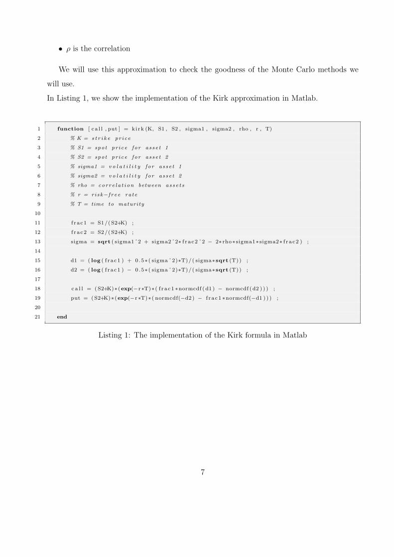
We will use this approximation to check the goodness of the Monte Carlo methods we

will use.

In Listing 1, we show the implementation of the Kirk approximation in Matlab.

1 function [ c a l l , put ] = k i rk (K, S1 , S2 , sigma1 , sigma2 , rho , r , T)

2 % K = s t r i k e p r i c e

3 % S1 = spot p r i c e f o r a s s e t 1


5 % sigma1 = v o l a t i l i t y f o r a s s e t 1


7 % rho = co r r e l a t i on between a s s e t s

8 % r = r i sk−f r e e ra t e

9 % T = time to maturi ty

10

11 f r a c 1 = S1/( S2+K) ;

12 f r a c 2 = S2/( S2+K) ;

13 sigma = sqrt ( sigma1ˆ2 + sigma2 ˆ2∗ f r a c 2 ˆ2 − 2∗ rho∗ sigma1∗ sigma2∗ f r a c 2 ) ;

14

15 d1 = ( log ( f r a c 1 ) + 0 . 5∗ ( sigma ˆ2)∗T)/( sigma∗sqrt (T) ) ;

16 d2 = ( log ( f r a c 1 ) − 0 . 5∗ ( sigma ˆ2)∗T)/( sigma∗sqrt (T) ) ;

17

18 c a l l = ( S2+K)∗ (exp(−r ∗T)∗ ( f r a c 1 ∗normcdf ( d1 ) − normcdf ( d2 ) ) ) ;

19 put = (S2+K)∗ (exp(−r ∗T)∗ ( normcdf(−d2 ) − f r a c 1 ∗normcdf(−d1 ) ) ) ;

20

21 end

Listing 1: The implementation of the Kirk formula in Matlab

7

2 Monte Carlo framework for pricing options

When pricing exotic options, very often a closed-form solution is not available. We thus

have to use some numerical methods. In the case of spread options, the following numerical

methods are available:

• Binomial or trinomial trees

• Finite differences (PDE solver)

• Monte Carlo methods

• FFT methods (in case we know the characteristic function for the underlying process,

which is always true with Levy processes for example)

For the scope of this project, we will focus on Monte Carlo methods.

Monte Carlo methods are famous for their simplicity but unfortunately also for their slow-

ness. However, a large number of variance reduction techniques exist that allow the method

to converge faster and then require less steps to be used.

Following, we present the basics of the Monte Carlo method.

When pricing an option under the Monte Carlo framework, we use the fact that an option

price can be written as the following discounted expectation

f(t) = e−r(T−t)EQ [φ(T )|Ft] (9)

where

• f(t) is the option price at date t < T

• r is the risk-free interest rate

• φ(T ) is the option payoff at date T

• Ft is the filtration representing the information set available at date t

• EQ is the expectation under the risk-neutral measure Q

8

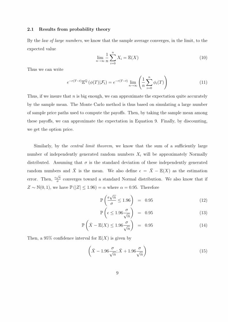
2.1 Results from probability theory

By the law of large numbers, we know that the sample average converges, in the limit, to the

expected value

limn→∞

1

n

n∑i=0

Xi = E(X) (10)

Thus we can write

e−r(T−t)EQ (φ(T )|Ft) = e−r(T−t) limn→∞

(1

n

n∑i=0

φi(T )

)(11)

Thus, if we insure that n is big enough, we can approximate the expectation quite accurately

by the sample mean. The Monte Carlo method is thus based on simulating a large number

of sample price paths used to compute the payoffs. Then, by taking the sample mean among

these payoffs, we can approximate the expectation in Equation 9. Finally, by discounting,

we get the option price.

Similarly, by the central limit theorem, we know that the sum of a sufficiently large

number of independently generated random numbers Xi will be approximately Normally

distributed. Assuming that σ is the standard deviation of these independently generated

random numbers and X is the mean. We also define ε = X − E(X) as the estimation

error. Then, ε√nσ

converges toward a standard Normal distribution. We also know that if

Z ∼ N(0, 1), we have P (|Z| ≤ 1.96) = α where α = 0.95. Therefore

P(ε√n

σ≤ 1.96

)= 0.95 (12)

P(ε ≤ 1.96

σ√n

)= 0.95 (13)

P(X − E(X) ≤ 1.96

σ√n

)= 0.95 (14)

Then, a 95% confidence interval for E(X) is given by(X − 1.96

σ√n

; X + 1.96σ√n

)(15)

9

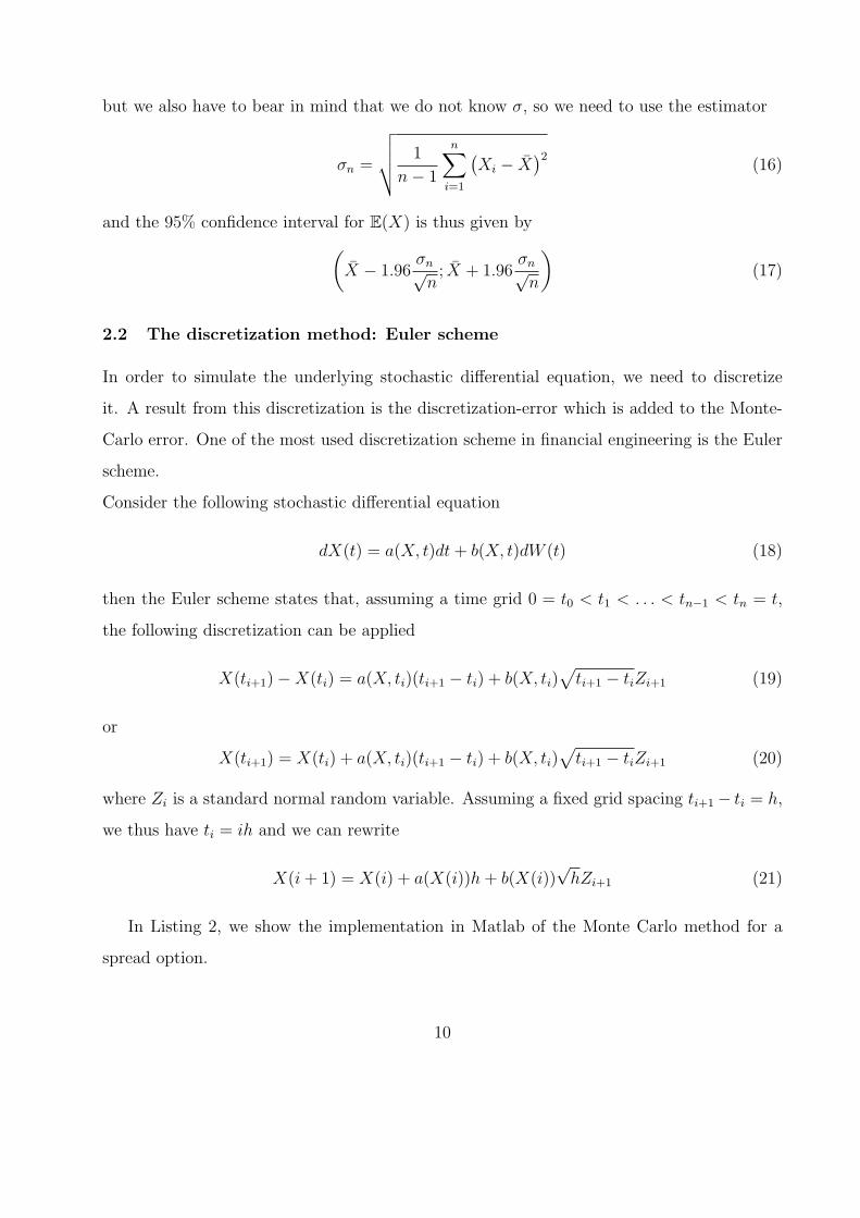
but we also have to bear in mind that we do not know σ, so we need to use the estimator

σn =

√√√√ 1

n− 1

n∑i=1

(Xi − X

)2(16)

and the 95% confidence interval for E(X) is thus given by(X − 1.96

σn√n

; X + 1.96σn√n

)(17)

2.2 The discretization method: Euler scheme

In order to simulate the underlying stochastic differential equation, we need to discretize

it. A result from this discretization is the discretization-error which is added to the Monte-

Carlo error. One of the most used discretization scheme in financial engineering is the Euler

scheme.

Consider the following stochastic differential equation

dX(t) = a(X, t)dt+ b(X, t)dW (t) (18)

then the Euler scheme states that, assuming a time grid 0 = t0 < t1 < . . . < tn−1 < tn = t,

the following discretization can be applied

X(ti+1)−X(ti) = a(X, ti)(ti+1 − ti) + b(X, ti)√ti+1 − tiZi+1 (19)

or

X(ti+1) = X(ti) + a(X, ti)(ti+1 − ti) + b(X, ti)√ti+1 − tiZi+1 (20)

where Zi is a standard normal random variable. Assuming a fixed grid spacing ti+1− ti = h,

we thus have ti = ih and we can rewrite

X(i+ 1) = X(i) + a(X(i))h+ b(X(i))√hZi+1 (21)

In Listing 2, we show the implementation in Matlab of the Monte Carlo method for a

spread option.

10

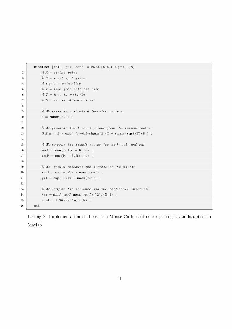
1 function [ c a l l , put , conf ] = BS MC(S ,K, r , sigma ,T,N)


3 % S = as s e t spot p r i c e

4 % sigma = v o l a t i l i t y

5 % r = r i sk−f r e e i n t e r e s t ra t e


7 % N = number o f s imu la t i ons

8

9 % We generate a standard Gaussian vec t o r s

10 Z = randn(N, 1 ) ;

11

12 % We generate f i n a l a s s e t p r i c e s from the random vec tor

13 S f i n = S ∗ exp( ( r−0.5∗ sigma ˆ2)∗T + sigma∗sqrt (T)∗Z ) ;

14

15 % We compute the payo f f v ec to r f o r both c a l l and put

16 resC = max( S f i n − K, 0) ;

17 resP = max(K − S f in , 0) ;

18

19 % We f i n a l l y d i scount the average o f the payo f f

20 c a l l = exp(−r ∗T) ∗ mean( resC ) ;

21 put = exp(−r ∗T) ∗ mean( resP ) ;

22

23 % We compute the var iance and the conf idence i n t e r v a l l

24 var = sum( ( resC−mean( resC ) . ˆ 2 ) / (N−1) ;

25 conf = 1.96∗ var /sqrt (N) ;

26 end

Listing 2: Implementation of the classic Monte Carlo routine for pricing a vanilla option in

Matlab

11

2.3 The spread option setting

When pricing spread options with the Monte Carlo method, we used the fact that the dy-

namics of both asset prices can be written as

dS1(t)

S1(t)= µ1(t, S1(t), S2(t))dt+ σ1(t, S1(t), S2(t)) (22)[

ρ(t, S1(t), S2(t))dW1(t) +√

1− ρ(t, S1(t), S2(t))dW2(t)]

dS2(t)

S2(t)= µ2(t, S1(t), S2(t))dt+ σ2(t, S1(t), S2(t))dW2(t) (23)

where

• S1,2 is the price of the asset 1, 2

• µ1,2 is the cost of carry for the asset 1, 2

• σ1,2 is the volatility for the asset 1, 2

• ρ is the correlation between both assets

The two equations can be solved separately and the solutions are as following

S1(T ) = S1(0) exp[(µ1 − σ2

1/2)T + σ1ρ√TU + σ2

√1− ρ2

√TV]

(24)

S2(T ) = S2(0) exp[(µ2 − σ2

2/2)T + σ2

√TU]

(25)

where U and V are two independent standard Gaussian random variables.

Then, we know that the payoff at maturity of a spread call option is defined as

ΦC(T ) = S1(T )− S2(T )−K (26)

and a spread put option

ΦP (T ) = K − [S1(T )− S2(T )] (27)

So, as explained in the previous section, given the value of the parameters and the asset

prices today S1(0) and S2(0), we can compute the option price at date t by simulation a large

number of asset prices S1(T ) and S2(T ) from Equations 24 and 25. We can then compute

12

the payoff from these simulations with Equations 26 and 27, take an average of it and finally

discount it in order to get the option price.

In Listing 3, we show the implementation in Matlab of the Monte Carlo method for a spread

option.

13

1 function [ c a l l , put , conf ] = MC(K, S1 , S2 , sigma1 , sigma2 , mu1 , mu2 , rho , r , T, N)






7 % mu1 = cos t o f carry f o r a s s e t 1

8 % mu2 = cos t o f carry f o r a s s e t 2





13

14 % We generate two standard Gaussian vec t o r s

15 U = randn(N, 1 ) ;

16 V = randn(N, 1 ) ;

17

18 % We generate f i n a l c o r r e l a t e d a s s e t p r i c e s from the 2 random vec to r s

19 S1 f i n = S1 ∗ exp( (mu1−0.5∗ sigma1 ˆ2)∗T + sigma1∗ rho∗sqrt (T)∗U + . . .

20 . . . + sigma2∗sqrt(1−rho ˆ2)∗ sqrt (T)∗V ) ;

21 S2 f i n = S2 ∗ exp( (mu2−0.5∗ sigma2 ˆ2)∗T + sigma2∗sqrt (T)∗U ) ;

22


24 resC = max( ( S 1 f i n − S2 f i n ) − K, 0) ;

25 resP = max(K − ( S 1 f i n − S2 f i n ) , 0) ;

26




30


32 var = sum( ( resC−meanC) . ˆ 2 ) / (N−1) ;

33 conf = 1.96∗ var /sqrt (N) ;

34 end

Listing 3: Implementation of the classic Monte Carlo routine for pricing a spread option in

Matlab

14

3 Variance reduction techniques

In order to increment the efficiency of Monte Carlo simulations, we need to reduce the variance

of the estimates.

We are presenting two variance reduction techniques: antithetic variates and control variates.

We first apply these techniques to vanilla options in order to compare their efficacy with the

Black-Scholes formula.

3.1 Antithetic variates

The method of antithetic variates reduces variance by introducing negative dependence be-

tween pairs of replications.

For example, when generating random variables normally distributed, the variables Z and

−Z form an antithetic pair since a large value of one results in a small value of the other. This

is due to the fact that the standard Normal distribution is symmetric around zero. Thus, if

we use the standard N(0, 1) i.i.d variables Zi in order to generate a Brownian motion path,

using −Zi we simulate the reflection of this path about the origin. Based upon this fact,

using this method we actually reduce the variance of the errors.

Assuming we want to price a vanilla option using the Monte Carlo numerical method

coupled with the antithetic variates method in order to reduce the variance, we have to

proceed as follows:

• we compute a vector Z1 of Normal random variables.

• we compute a vector of asset prices S1 under the GBM process based on the vector Z1

• we create a new vector Z2 given by Z2 = −Z1

• we compute a new vector of asset prices S2 under the GBM process based on the vector

Z2

15

• we take an average of the values constituting both vectors S1 and S2 that we call A1

and A2

• we take the following average (A1 + A2)/2 and we discount it.

In Listing 4, we show the implementation in Matlab of the Monte Carlo method for pric-

ing a vanilla option using the antithetic variates for reducing the variance of the estimates.

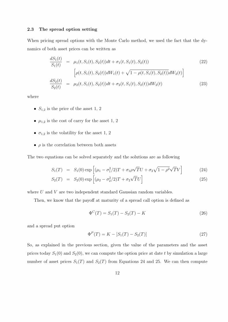
In Figure 1, we show the convergence of the Monte Carlo option prices to the actual

Black-Scholes price using both the classic Monte Carlo method and the Monte Carlo method

coupled with the antithetic variates. We clearly see that even if both seem to converge to

the same value, the variance of the second one is lower and the price converges a lot faster.

Figure 1: Evolution of the Monte Carlo option price when the number of simulations in-

creases. Using antithetic variates (red), we see the Monte Carlo price converges earlier.

16

1 function [ c a l l , put , conf ] = antitheticBS MC (S ,K, r , sigma ,T,N)

2 % S = spor t p r i c e






8

9 % We generate a standard Gaussian vec tor

10 Z = randn(N, 1 ) ;

11 % We generate the a n t i t h e t i c random vec tor

12 nZ = −Z ;

13

14 % We generate f i n a l a s s e t p r i c e s from both random vec to r s

15 pS f i n = S ∗ exp ( ( r−0.5∗ sigma ˆ2)∗T + sigma∗sqrt (T)∗Z ) ;

16 nS f i n = S ∗ exp ( ( r−0.5∗ sigma ˆ2)∗T + sigma∗sqrt (T)∗nZ ) ;

17

18 % We compute the payo f f v ec to r f o r the c a l l f o r both random vec to r s

19 resCp = max( pS f i n − K, 0) ;

20 resCn = max( nS f i n − K, 0) ;

21 % We compute the payo f f v ec to r f o r the put f o r both random vec to r s

22 resPp = max(K − pS f in , 0) ;

23 resPn = max(K − nS f in , 0) ;

24

25 % We compute the average between normal and a n t i t h e t i c payo f f s

26 resC = 0 .5 ∗ ( resCp + resCn ) ;

27 resP = 0 .5 ∗ ( resPp + resPn ) ;

28


30 c a l l = exp(−r ∗T)∗mean( resC ) ;

31 put = exp(−r ∗T)∗mean( resP ) ;

32


34 var = sum( ( resC−meanC) . ˆ 2 ) / (N−1) ;

35 conf = 1.96∗ var /sqrt (N) ;

36 end

Listing 4: Matlab function that computes vanilla option prices with Monte Carlo using

antithetic variates variance reduction technique.

17

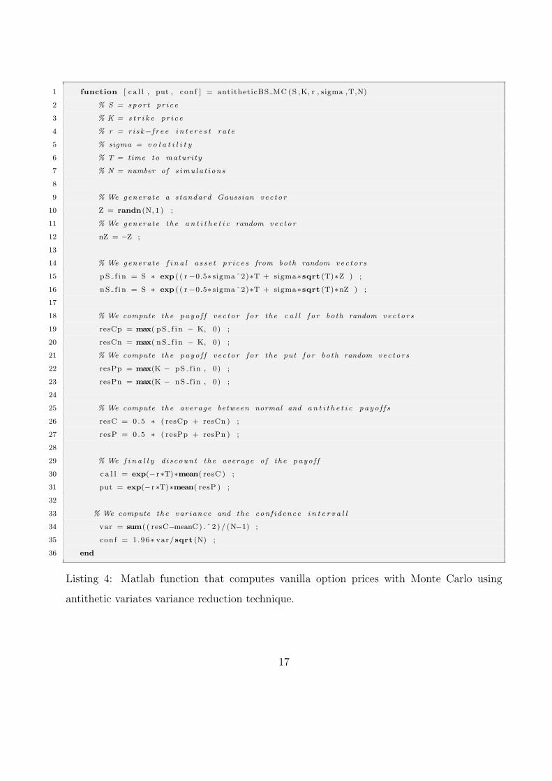
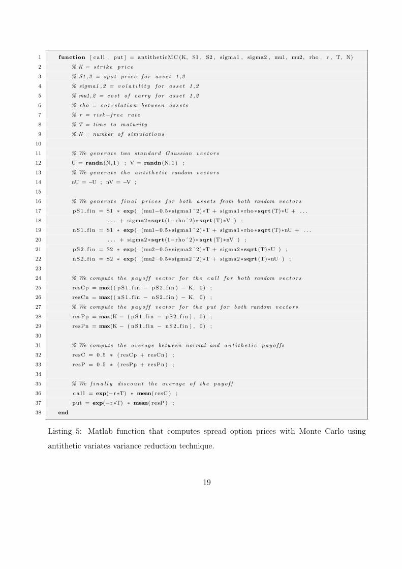
In Listing 5 we show the Matlab implementation of the Monte Carlo method for pricing

a spread option using the antithetic variates variance reduction technique.

3.2 Control variates

The control variate technique allows an effective variance reduction in a simple theoretical

framework. The method takes advantage of random variables with known expected value

and positively correlated with the variable under consideration. Let Y be a random variable

whose mean is to be determined through Monte Carlo simulation and X a random variable

with known mean E(X). Now, for each trial, the outcome of Xi is calculated along with the

output of Yi. Let us call Y CV the control variate estimator of E(Y ). The control variate

estimator is thus given by

Y CV =1

n

n∑i=1

(Yi − b(Xi − E(X))) (28)

= Y − b(X − E(X)) (29)

for any fixed b (further we will talk about the estimation of this parameter b).

We can show that the control variate estimator YCV is unbiased and consistent

E(Y CV ) = E(Y )− E(X) + E(X) = E(Y ) (30)

and

limn→∞

1

n

n∑i=1

Y CVi = lim

n→∞

1

n

n∑i=1

(Yi −Xi + E(X)) = E(Y −X + E(X))→ E(Y ) (31)

Then, each Yi has variance

var(Y CVi ) = var(Yi − b[Xi − E(X)]) (32)

= σ2Y − 2bσXσY ρ+ b2σ2

X (33)

where σ2X = var(X), σ2

Y = var(Y ) and ρ is the correlation between X and Y .

The optimal coefficient b∗ that minimizes the variance is given by

b∗ =σYσX

ρ =cov(X, Y )

var(X)(34)

18

1 function [ c a l l , put ] = antitheticMC (K, S1 , S2 , sigma1 , sigma2 , mu1 , mu2 , rho , r , T, N)


3 % S1 ,2 = spot p r i c e f o r a s s e t 1 ,2

4 % sigma1 ,2 = v o l a t i l i t y f o r a s s e t 1 ,2

5 % mu1,2 = cos t o f carry f o r a s s e t 1 ,2





10

11 % We generate two standard Gaussian vec t o r s

12 U = randn(N, 1 ) ; V = randn(N, 1 ) ;

13 % We generate the a n t i t h e t i c random vec to r s

14 nU = −U ; nV = −V ;

15

16 % We generate f i n a l p r i c e s f o r both a s s e t s from both random vec to r s

17 pS1 f i n = S1 ∗ exp( (mu1−0.5∗ sigma1 ˆ2)∗T + sigma1∗ rho∗sqrt (T)∗U + . . .

18 . . . + sigma2∗sqrt(1−rho ˆ2)∗ sqrt (T)∗V ) ;

19 nS1 f i n = S1 ∗ exp( (mu1−0.5∗ sigma1 ˆ2)∗T + sigma1∗ rho∗sqrt (T)∗nU + . . .

20 . . . + sigma2∗sqrt(1−rho ˆ2)∗ sqrt (T)∗nV ) ;

21 pS2 f i n = S2 ∗ exp( (mu2−0.5∗ sigma2 ˆ2)∗T + sigma2∗sqrt (T)∗U ) ;

22 nS2 f i n = S2 ∗ exp( (mu2−0.5∗ sigma2 ˆ2)∗T + sigma2∗sqrt (T)∗nU ) ;

23

24 % We compute the payo f f v ec to r f o r the c a l l f o r both random vec to r s

25 resCp = max( ( pS1 f i n − pS2 f i n ) − K, 0) ;

26 resCn = max( ( nS1 f i n − nS2 f i n ) − K, 0) ;

27 % We compute the payo f f v ec to r f o r the put f o r both random vec to r s

28 resPp = max(K − ( pS1 f i n − pS2 f i n ) , 0) ;

29 resPn = max(K − ( nS1 f i n − nS2 f i n ) , 0) ;

30

31 % We compute the average between normal and a n t i t h e t i c payo f f s

32 resC = 0 .5 ∗ ( resCp + resCn ) ;

33 resP = 0 .5 ∗ ( resPp + resPn ) ;

34




38 end

Listing 5: Matlab function that computes spread option prices with Monte Carlo using

antithetic variates variance reduction technique.

19

Since we do not know the values of cov(X, Y ) and var(X), we have to estimate b∗ as follows

b∗ =

∑ni=1(Xi − X)(Yi − Y )∑n

i=1(Xi − X)2(35)

As a control variate, we can use the underlying asset for example. Since we know that

discounted asset prices are martingale

E(S(T )) = erTS(0) (36)

we can easily use S as the control variate and, assuming φ is the payoff of the option, we can

write the control variate estimator as

1

n

n∑i=1

(φi − b[Si(T )− erTS(0)]) (37)

In Listing 6, we show the implementation in Matlab of the Monte Carlo method for pric-

ing a vanilla option using the control variates for reducing the variance of the estimates.

In Figure 2, we show the convergence of the Monte Carlo option prices to the actual

Black-Scholes price using both the classic Monte Carlo method and the Monte Carlo method

coupled with the control variates. We clearly see that even if both seem to converge to the

same value, the variance of the second one is lower and the price converges a lot faster.

20

1 function [ c a l l , put ] = controlBS MC (S ,K, r , sigma ,T,N)

2 % S = spor t p r i c e






8

9 % We generate a standard Gaussian vec tor

10 Z = randn(N, 1 ) ;

11

12 % We generate f i n a l a s s e t p r i c e s from the random vec tor

13 S f i n = S∗exp ( ( r−0.5∗ sigma ˆ2)∗T + sigma∗sqrt (T)∗Z) ;

14


16 resC = max( S f i n − K, 0) ;

17 resP = max(K − S f in , 0) ;

18

19 % We sub s t r a c t the mean to each payo f f

20 newC = resC − mean( resC ) ;

21 newP = resP − mean( resP ) ;

22 % We sub s t r a c t the mean to each f i n a l p r i c e

23 newS = S f i n − mean( S f i n ) ;

24

25 % We compute the va lue o f be ta f o r both c a l l and put

26 bC = mean(newC.∗newS)/mean(newS .∗newS) ;

27 bP = mean(newP .∗newS)/mean(newS .∗newS) ;

28

29 % We compute the payo f f c on t ro l v a r i a t e s

30 f i na lC = resC − bC∗( S f i n − exp( r ∗T)∗S) ;

31 f i n a lP = resP − bP∗( S f i n − exp( r ∗T)∗S) ;

32


34 c a l l = exp(−r ∗T) ∗ mean( f i na lC ) ;

35 put = exp(−r ∗T) ∗ mean( f i n a lP ) ;

36 end

Listing 6: Matlab function that computes vanilla option prices with Monte Carlo using control

variates variance reduction technique.

21

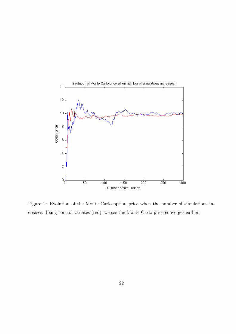
Figure 2: Evolution of the Monte Carlo option price when the number of simulations in-

creases. Using control variates (red), we see the Monte Carlo price converges earlier.

22

4 Results

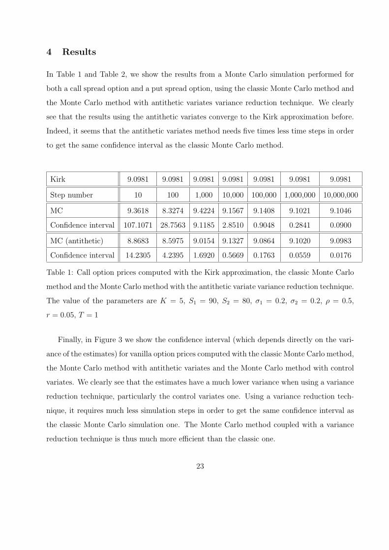
In Table 1 and Table 2, we show the results from a Monte Carlo simulation performed for

both a call spread option and a put spread option, using the classic Monte Carlo method and

the Monte Carlo method with antithetic variates variance reduction technique. We clearly

see that the results using the antithetic variates converge to the Kirk approximation before.

Indeed, it seems that the antithetic variates method needs five times less time steps in order

to get the same confidence interval as the classic Monte Carlo method.

Kirk 9.0981 9.0981 9.0981 9.0981 9.0981 9.0981 9.0981

Step number 10 100 1,000 10,000 100,000 1,000,000 10,000,000

MC 9.3618 8.3274 9.4224 9.1567 9.1408 9.1021 9.1046

Confidence interval 107.1071 28.7563 9.1185 2.8510 0.9048 0.2841 0.0900

MC (antithetic) 8.8683 8.5975 9.0154 9.1327 9.0864 9.1020 9.0983


Table 1: Call option prices computed with the Kirk approximation, the classic Monte Carlo

method and the Monte Carlo method with the antithetic variate variance reduction technique.

The value of the parameters are K = 5, S1 = 90, S2 = 80, σ1 = 0.2, σ2 = 0.2, ρ = 0.5,

r = 0.05, T = 1

Finally, in Figure 3 we show the confidence interval (which depends directly on the vari-

ance of the estimates) for vanilla option prices computed with the classic Monte Carlo method,

the Monte Carlo method with antithetic variates and the Monte Carlo method with control

variates. We clearly see that the estimates have a much lower variance when using a variance

reduction technique, particularly the control variates one. Using a variance reduction tech-

nique, it requires much less simulation steps in order to get the same confidence interval as

the classic Monte Carlo simulation one. The Monte Carlo method coupled with a variance

reduction technique is thus much more efficient than the classic one.

23

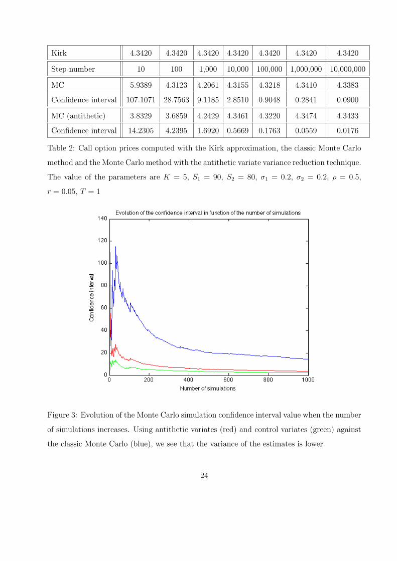
Kirk 4.3420 4.3420 4.3420 4.3420 4.3420 4.3420 4.3420

Step number 10 100 1,000 10,000 100,000 1,000,000 10,000,000

MC 5.9389 4.3123 4.2061 4.3155 4.3218 4.3410 4.3383


MC (antithetic) 3.8329 3.6859 4.2429 4.3461 4.3220 4.3474 4.3433


Table 2: Call option prices computed with the Kirk approximation, the classic Monte Carlo

method and the Monte Carlo method with the antithetic variate variance reduction technique.

The value of the parameters are K = 5, S1 = 90, S2 = 80, σ1 = 0.2, σ2 = 0.2, ρ = 0.5,

r = 0.05, T = 1

Figure 3: Evolution of the Monte Carlo simulation confidence interval value when the number

of simulations increases. Using antithetic variates (red) and control variates (green) against

the classic Monte Carlo (blue), we see that the variance of the estimates is lower.

24

5 Conclusion

We first presented the spread options and exposed their characteristics. We then explained

the Monte Carlo framework for pricing vanilla options and showed how it could be extended

in order to price exotic options, spread options in particular. We wrote some Matlab code

that replicates these methods and compute option prices with the Monte Carlo framework.

Finally, in order to increase the efficiency of the Monte Carlo method, we presented two

variance reduction techniques: the antithetic variates and the control variates. We showed

how these techniques actually decreased the variance of the estimates increasing radically the

efficiency of the Monte Carlo method since much less steps were required in order to get the

same result as a classic Monte Carlo method.

Some extensions to this project could be the introduction of a stochastic interest rate or a

stochastic volatility in the model. We could also use other types of stochastic processes for

the underlying such as processes displaying jumps as the Levy processes.

25

Appendix

A Additional Matlab code

In this appendix, we list the Matlab code that has been used in order to generate the graphs.

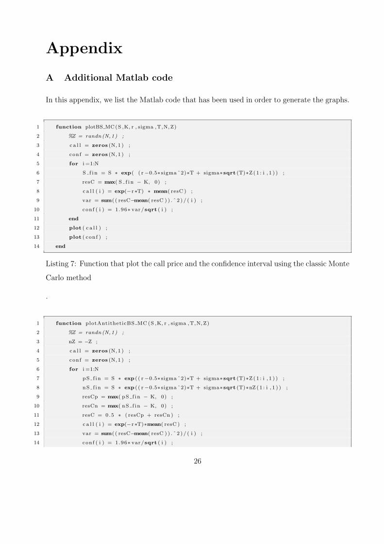
1 function plotBS MC(S ,K, r , sigma ,T,N,Z)

2 %Z = randn (N,1 ) ;

3 c a l l = zeros (N, 1 ) ;

4 conf = zeros (N, 1 ) ;

5 for i =1:N

6 S f i n = S ∗ exp( ( r−0.5∗ sigma ˆ2)∗T + sigma∗sqrt (T)∗Z ( 1 : i , 1 ) ) ;

7 resC = max( S f i n − K, 0) ;

8 c a l l ( i ) = exp(−r ∗T) ∗ mean( resC ) ;

9 var = sum( ( resC−mean( resC ) ) . ˆ 2 ) / ( i ) ;

10 conf ( i ) = 1.96∗ var /sqrt ( i ) ;

11 end

12 plot ( c a l l ) ;

13 plot ( conf ) ;

14 end

Listing 7: Function that plot the call price and the confidence interval using the classic Monte

Carlo method

.

1 function plotAntitheticBS MC (S ,K, r , sigma ,T,N,Z)

2 %Z = randn (N,1 ) ;

3 nZ = −Z ;

4 c a l l = zeros (N, 1 ) ;


6 for i =1:N

7 pS f i n = S ∗ exp ( ( r−0.5∗ sigma ˆ2)∗T + sigma∗sqrt (T)∗Z ( 1 : i , 1 ) ) ;

8 nS f i n = S ∗ exp ( ( r−0.5∗ sigma ˆ2)∗T + sigma∗sqrt (T)∗nZ ( 1 : i , 1 ) ) ;

9 resCp = max( pS f i n − K, 0) ;

10 resCn = max( nS f i n − K, 0) ;

11 resC = 0 .5 ∗ ( resCp + resCn ) ;

12 c a l l ( i ) = exp(−r ∗T)∗mean( resC ) ;

13 var = sum( ( resC−mean( resC ) ) . ˆ 2 ) / ( i ) ;

14 conf ( i ) = 1.96∗ var /sqrt ( i ) ;

26

15 end

16 plot ( c a l l , ’ r ’ ) ;

17 plot ( conf , ’ r ’ ) ;

18 end

Listing 8: Function that plot the call price and the confidence interval using the Monte Carlo

method with the antithetic variates

.

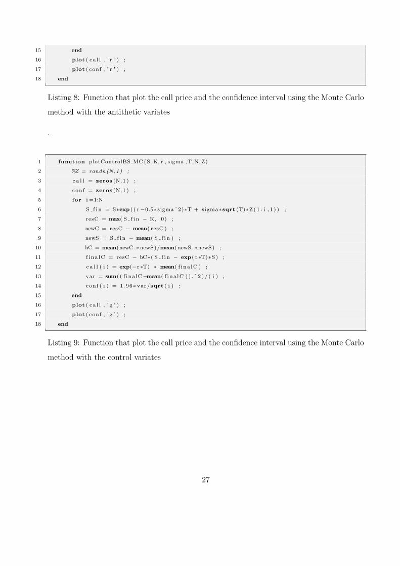
1 function plotControlBS MC (S ,K, r , sigma ,T,N,Z)

2 %Z = randn (N,1 ) ;

3 c a l l = zeros (N, 1 ) ;


5 for i =1:N

6 S f i n = S∗exp ( ( r−0.5∗ sigma ˆ2)∗T + sigma∗sqrt (T)∗Z ( 1 : i , 1 ) ) ;

7 resC = max( S f i n − K, 0) ;

8 newC = resC − mean( resC ) ;

9 newS = S f i n − mean( S f i n ) ;

10 bC = mean(newC.∗newS)/mean(newS .∗newS) ;

11 f i na lC = resC − bC∗( S f i n − exp( r ∗T)∗S) ;

12 c a l l ( i ) = exp(−r ∗T) ∗ mean( f i na lC ) ;

13 var = sum( ( f ina lC−mean( f i na lC ) ) . ˆ 2 ) / ( i ) ;

14 conf ( i ) = 1.96∗ var /sqrt ( i ) ;

15 end

16 plot ( c a l l , ’ g ’ ) ;

17 plot ( conf , ’ g ’ ) ;

18 end

Listing 9: Function that plot the call price and the confidence interval using the Monte Carlo

method with the control variates

27

References

[1] Andreas, A., Engelmann, B., Schwendner, P., and Wystup, U. Fast fourier

method for the valuation of options on several correlated currencies. Foreign Exchange

Risk 2 (2002).

[2] Bjerksund, P., and Stensland, G. Closed form spread option valuation. pa-

pers.ssrn.com (2006).

[3] Black, F. The pricing of commodity contracts. Journal of financial economics (1976),

167–179.

[4] Boyle, P. P. A lattice framework for option pricing with two state variables. Journal

of Financial and Quantitative Analysis (1988), 1–12.

[5] Carmona, R., and Durrleman, V. Pricing and hedging spread options. Siam

Review 45, 4 (2003), 627–685.

[6] Carmona, R., and Durrleman, V. Pricing and hedging spread options in a lognor-

mal model. Siam Review 45, 4 (2003), 627–685.

[7] Dempster, M., and Hong, S. Spread option valuation and the fast fourier transform.

manuscript. University of Cambridge (2000).

[8] Duan, J., and Pliska, S. Option valuation with co-integrated asset prices. Journal

of Economic Dynamics and Control 28, 4 (2004), 727–754.

[9] Geman, H. Commodities and commodity derivatives. Wiley, 2005.

[10] Glasserman, P. Monte Carlo methods in financial engineering. Springer, 2003.

[11] Margrabe, W. The value of an option to exchange one asset for another. Journal of

Finance (1978), 177–186.

28

[12] Nakajima, K., and Maeda, A. Pricing commodity spread options with stochastic

term structure of convenience yields and interest rates. Asia-Pacific Finan Markets 14,

1 (2007), 157–184.

29

Documents

Commodity Spread Option Pricing