COMMON MISTAKES ON THE AP MICRO EXAM

Compiled by: John Ostick

Malvern PrepMalvern, PA 19355

COMMON MISTAKES ON THE AP MICRO EXAM

Compiled by: John Ostick

Malvern PrepMalvern, PA 19355

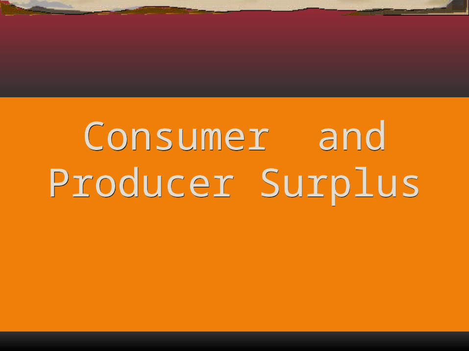
Consumer and Producer SurplusConsumer and

Producer Surplus

McGraw-Hill/Irwin © 2002 The McGraw-Hill Companies, Inc., All Rights Reserved.

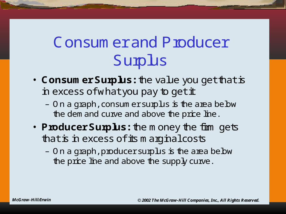
Consumer and Producer Surplus

• Consumer Surplus: the value you get that is in excess of what you pay to get it – On a graph, consumer surplus is the area below

the demand curve and above the price line.

• Producer Surplus: the money the firm gets that is in excess of its marginal costs– On a graph, producer surplus is the area below

the price line and above the supply curve.

McGraw-Hill/Irwin © 2002 The McGraw-Hill Companies, Inc., All Rights Reserved.

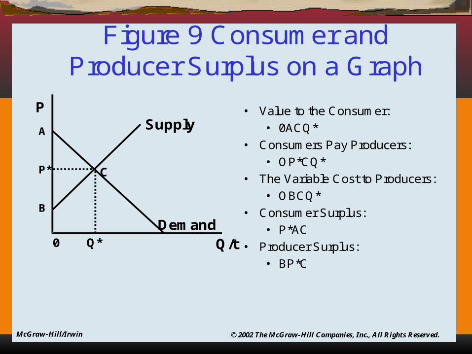
Figure 9 Consumer and Producer Surplus on a Graph

Q/t

P

Demand

SupplyA

P*

B

C

0 Q*

• Value to the Consumer:

• 0ACQ*

• Consumers Pay Producers:

• OP*CQ*

• The Variable Cost to Producers:

• OBCQ*

• Consumer Surplus:

• P*AC

• Producer Surplus:

• BP*C

Dead Weight LossDead Weight Loss

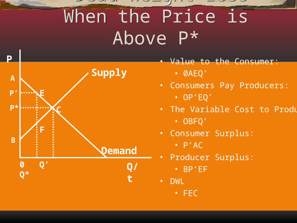
Dead Weight Loss When the Price is Above P*

Dead Weight Loss When the Price is Above P*

Q/t

P

Demand

SupplyA

C

0 Q’ Q*

E

F

P’

P*

B

• Value to the Consumer: • 0AEQ’

• Consumers Pay Producers: • OP’EQ’

• The Variable Cost to Producers: • OBFQ’

• Consumer Surplus: • P’AC

• Producer Surplus: • BP’EF

• DWL• FEC

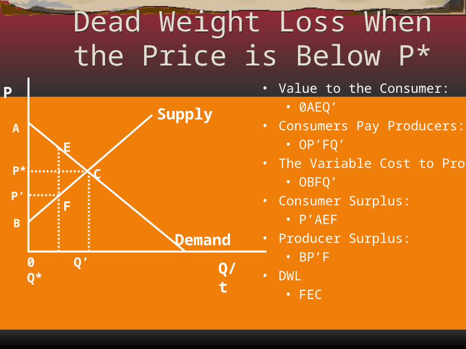
Dead Weight Loss When the Price is Below P*

Dead Weight Loss When the Price is Below P*

Q/t

P

Demand

SupplyA

P* C

0 Q’ Q*

E

FP’

B

• Value to the Consumer: • 0AEQ’

• Consumers Pay Producers: • OP’FQ’

• The Variable Cost to Producers: • OBFQ’

• Consumer Surplus: • P’AEF

• Producer Surplus: • BP’F

• DWL• FEC

ELASTICITY

Tax Incidence &

Effects on Revenue and Prices

ELASTICITY

Tax Incidence &

Effects on Revenue and Prices

Tax RevenuesEfficiency Loss of a TaxRole of ElasticitiesQualifications

•Redistributive Goals•Reducing Negative Externalities

TAX INCIDENCE ANDEFFICIENCY LOSS

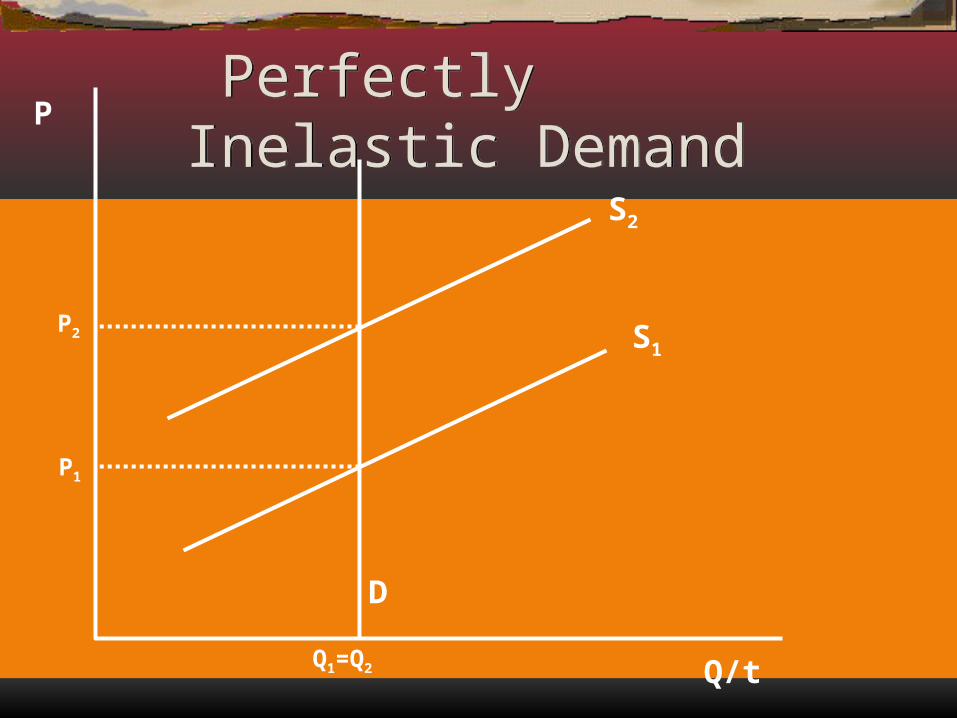
Perfectly Inelastic Demand Perfectly Inelastic Demand

D

Q/t

P

S2

Q1=Q2

P2 S1

P1

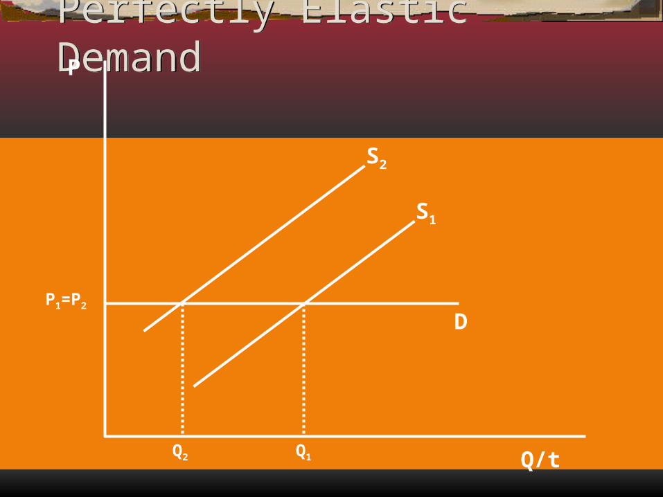
Perfectly Elastic Demand Perfectly Elastic Demand

Q/t

P

D

S2

P1=P2

Q2

S1

Q1

Inelastic Demand (at moderate prices)

Inelastic Demand (at moderate prices)

P

Q/t

D

S1

P1

Q1Q2

S2

P2

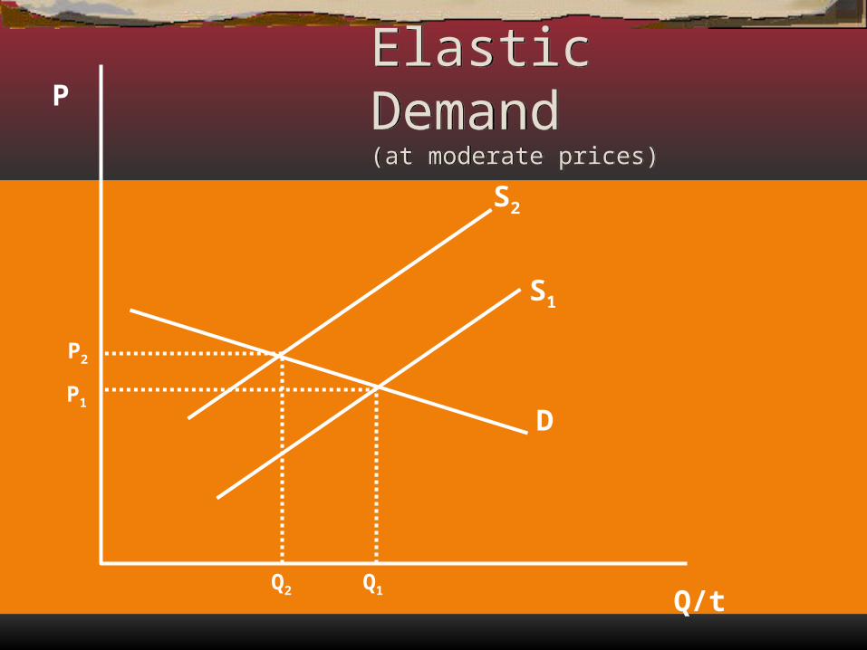
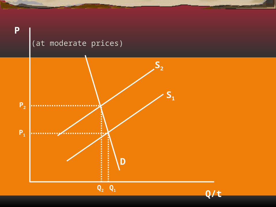
Elastic Demand(at moderate prices)

Elastic Demand(at moderate prices)

Q/t

P

Q1

D

S1

P1

S2

P2

Q2

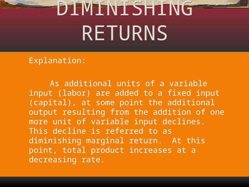
DIMINISHING RETURNS

DIMINISHING RETURNS

Explanation:

As additional units of a variable input (labor) are added to a fixed input (capital), at some point the additional output resulting from the addition of one more unit of variable input declines. This decline is referred to as diminishing marginal return. At this point, total product increases at a decreasing rate.

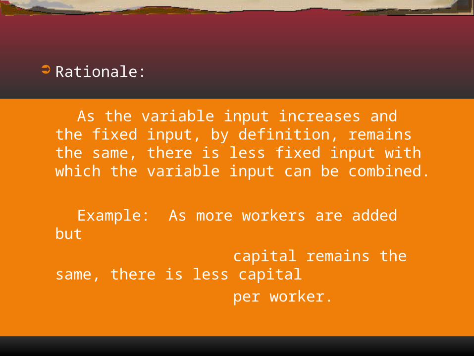
Rationale:

As the variable input increases and the fixed input, by definition, remains the same, there is less fixed input with which the variable input can be combined.

Example: As more workers are added but capital remains the same, there is less capital per worker.

Law of Diminishing Returns

SHORT-RUN PRODUCTIONRELATIONSHIPS

To

tal P

rod

uct

, TP

Quantity of Labor

Ave

rag

e P

rod

uct

, AP

, an

dm

arg

inal

pro

du

ct, M

P

Quantity of Labor

Total Product

MarginalProduct

AverageProduct

IncreasingMarginalReturns

Law of Diminishing Returns

SHORT-RUN PRODUCTIONRELATIONSHIPS

To

tal P

rod

uct

, TP

Quantity of Labor

Ave

rag

e P

rod

uct

, AP

, an

dm

arg

inal

pro

du

ct, M

P

Quantity of Labor

Total Product

MarginalProduct

AverageProduct

DiminishingMarginalReturns

Law of Diminishing Returns

SHORT-RUN PRODUCTIONRELATIONSHIPS

To

tal P

rod

uct

, TP

Quantity of Labor

Ave

rag

e P

rod

uct

, AP

, an

dm

arg

inal

pro

du

ct, M

P

Quantity of Labor

Total Product

MarginalProduct

AverageProduct

NegativeMarginalReturns

Two Approaches to Find the PROFIT

MAXIMIZING QUANTITY ( PRICE)

Two Approaches to Find the PROFIT

MAXIMIZING QUANTITY ( PRICE)

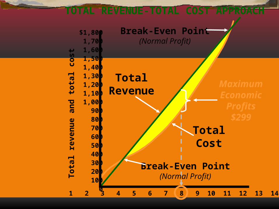
$1,8001,7001,6001,5001,4001,3001,2001,1001,000 900 800 700 600 500 400 300 200 100 0

To

tal r

eve

nu

e a

nd

to

tal c

ost

TotalRevenue

TotalCost

MaximumEconomic

Profits$299

Break-Even Point(Normal Profit)

Break-Even Point(Normal Profit)

1 2 3 4 5 6 7 8 9 10 11 12 13 14

TOTAL REVENUE-TOTAL COST APPROACH

$200

150

100

50

0

Co

st a

nd

Rev

enu

e

1 2 3 4 5 6 7 8 9 10

MC

MR

AVCATC

Economic Profit

$131.00

$97.78

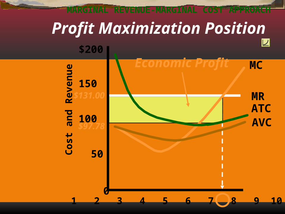
MARGINAL REVENUE-MARGINAL COST APPROACH

Profit Maximization Position

Key Micro FormulasKey Micro Formulas

 

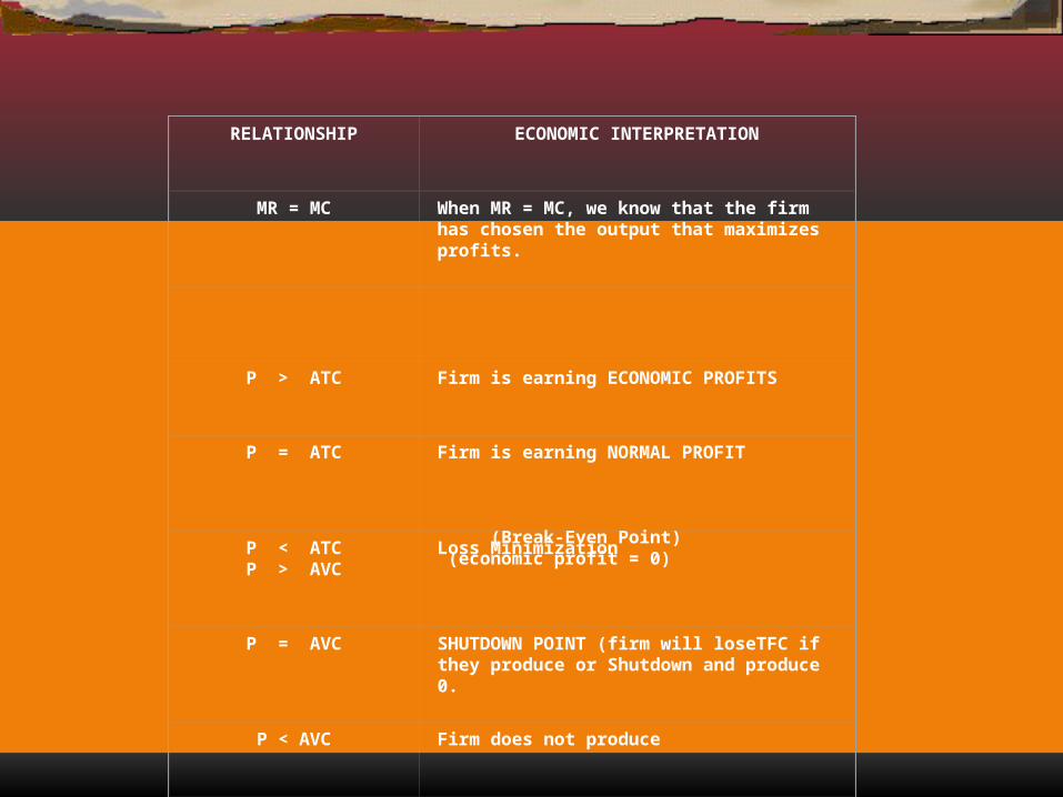
RELATIONSHIP ECONOMIC INTERPRETATION

MR = MC When MR = MC, we know that the firm has chosen the output that maximizes profits.

P > ATC Firm is earning ECONOMIC PROFITS

P = ATC Firm is earning NORMAL PROFIT (Break-Even Point) (economic profit = 0)

P < ATCP > AVC

Loss Minimization

P = AVC SHUTDOWN POINT (firm will loseTFC if they produce or Shutdown and produce 0.

P < AVC Firm does not produce

Finding the Perfectly

Competitive Firm’s Supply Curve

Finding the Perfectly

Competitive Firm’s Supply Curve

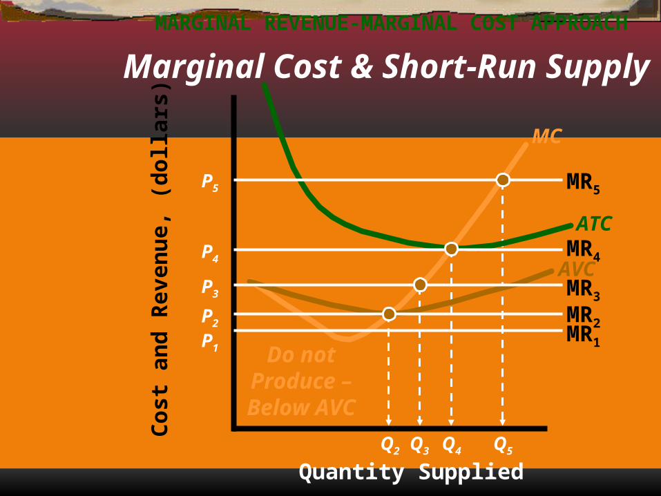
Co

st a

nd

Rev

enu

e, (

do

llar

s) MC

MR1

AVC

ATC

MARGINAL REVENUE-MARGINAL COST APPROACH

Quantity Supplied

MR2

MR3

MR4

MR5

P1

P2

P3

P4

P5

Q2 Q3 Q4 Q5

Marginal Cost & Short-Run Supply

Do notProduce –

Below AVC

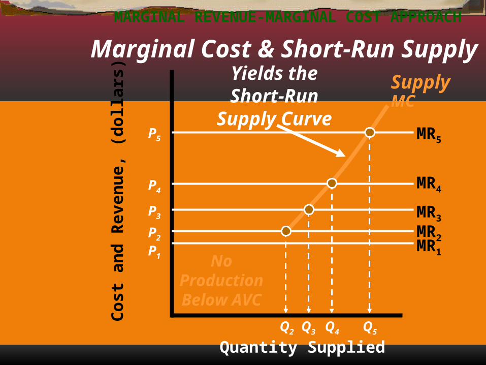
Co

st a

nd

Rev

enu

e, (

do

llar

s)MC

MR1

MARGINAL REVENUE-MARGINAL COST APPROACH

Quantity Supplied

MR2

MR3

MR4

MR5

P1

P2

P3

P4

P5

Q2 Q3 Q4 Q5

Marginal Cost & Short-Run SupplyYields theShort-Run

Supply Curve

Supply

NoProductionBelow AVC

Long Run Equilibrium (Perfectly

Competitive Firm)

Long Run Equilibrium (Perfectly

Competitive Firm) Productive Efficiency Allocative Efficiency

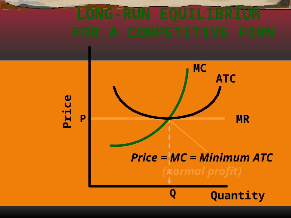
P MR

Q

MCATC

Quantity

Pri

ce

Price = MC = Minimum ATC(normal profit)

LONG-RUN EQUILIBRIUM FOR A COMPETITIVE FIRM

How an Increase in Demand Changes

Long-Run Equilibrium for the Firm and Industry

How an Increase in Demand Changes

Long-Run Equilibrium for the Firm and Industry

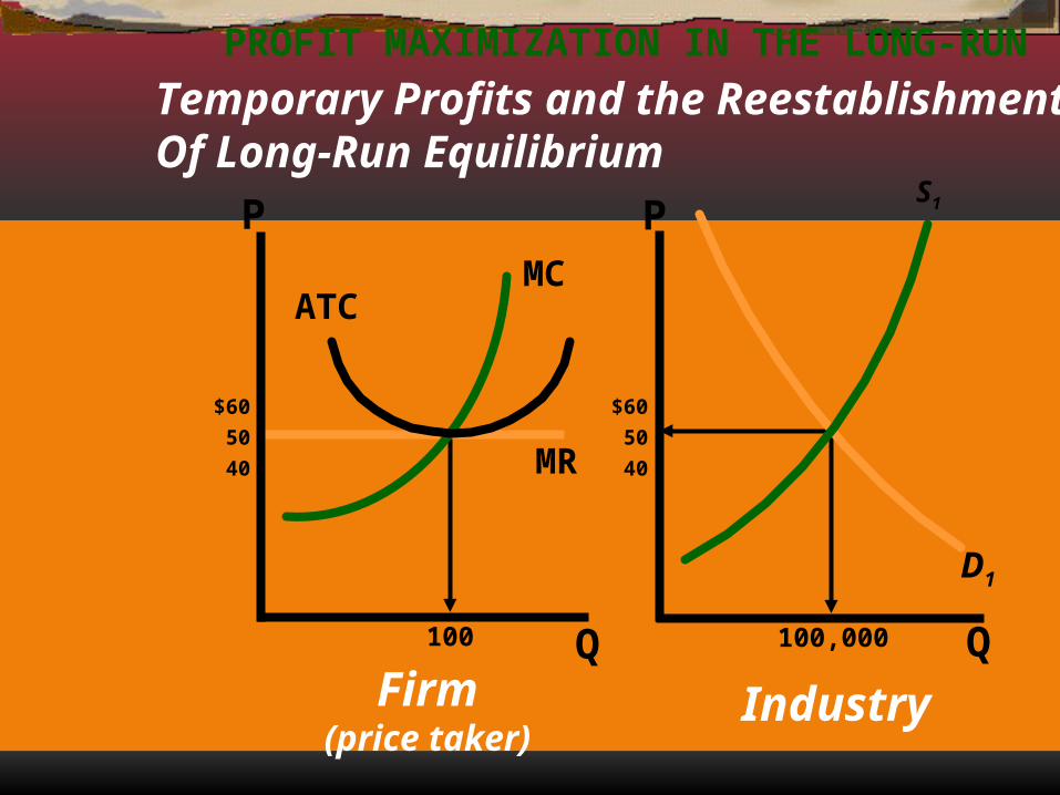
Temporary Profits and the ReestablishmentOf Long-Run Equilibrium

S1

MCATC

P

Q100

P

Q100,000

IndustryFirm(price taker)

$60

50

40

$60

50

40

PROFIT MAXIMIZATION IN THE LONG-RUN

MR

D1

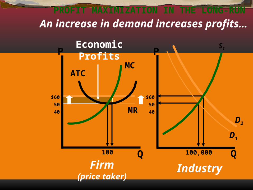
An increase in demand increases profits…

MR

D1

MCATC

P

Q100

P

Q100,000

IndustryFirm(price taker)

$60

50

40

$60

50

40

PROFIT MAXIMIZATION IN THE LONG-RUN

D2

EconomicProfits

S1

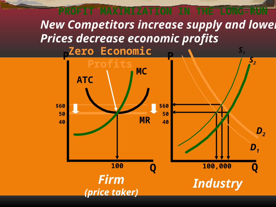
New Competitors increase supply and lowerPrices decrease economic profits

MR

D1

MCATC

P

Q100

P

Q100,000

IndustryFirm(price taker)

$60

50

40

$60

50

40

PROFIT MAXIMIZATION IN THE LONG-RUN

D2

Zero EconomicProfits

S1

S2

How an Decrease in Demand Changes Long-Run Equilibrium for the Firm and Industry

How an Decrease in Demand Changes Long-Run Equilibrium for the Firm and Industry

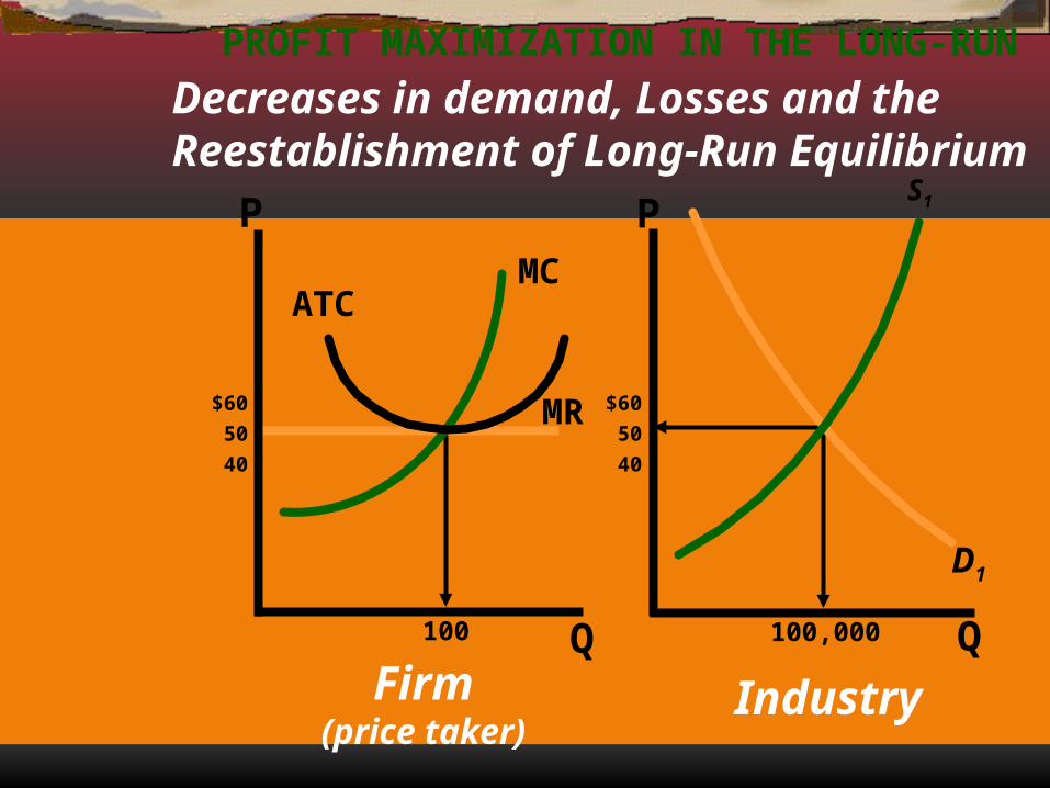
Decreases in demand, Losses and the Reestablishment of Long-Run Equilibrium

S1

MCATC

P

Q100

P

Q100,000

IndustryFirm(price taker)

$60

50

40

$60

50

40

PROFIT MAXIMIZATION IN THE LONG-RUN

D1

MR

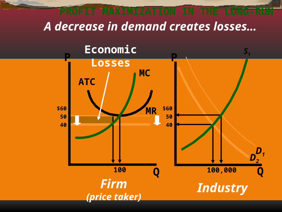
A decrease in demand creates losses…

MR

D1

MCATC

P

Q100

P

Q100,000

IndustryFirm(price taker)

$60

50

40

$60

50

40

PROFIT MAXIMIZATION IN THE LONG-RUN

D2

EconomicLosses

S1

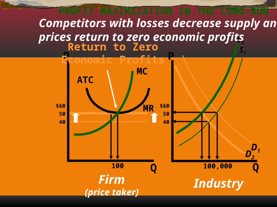
MR

D1

MCATC

P

Q100

P

Q100,000

IndustryFirm(price taker)

$60

50

40

$60

50

40

PROFIT MAXIMIZATION IN THE LONG-RUN

D2

Return to ZeroEconomic Profits

S1

S3

Competitors with losses decrease supply andprices return to zero economic profits

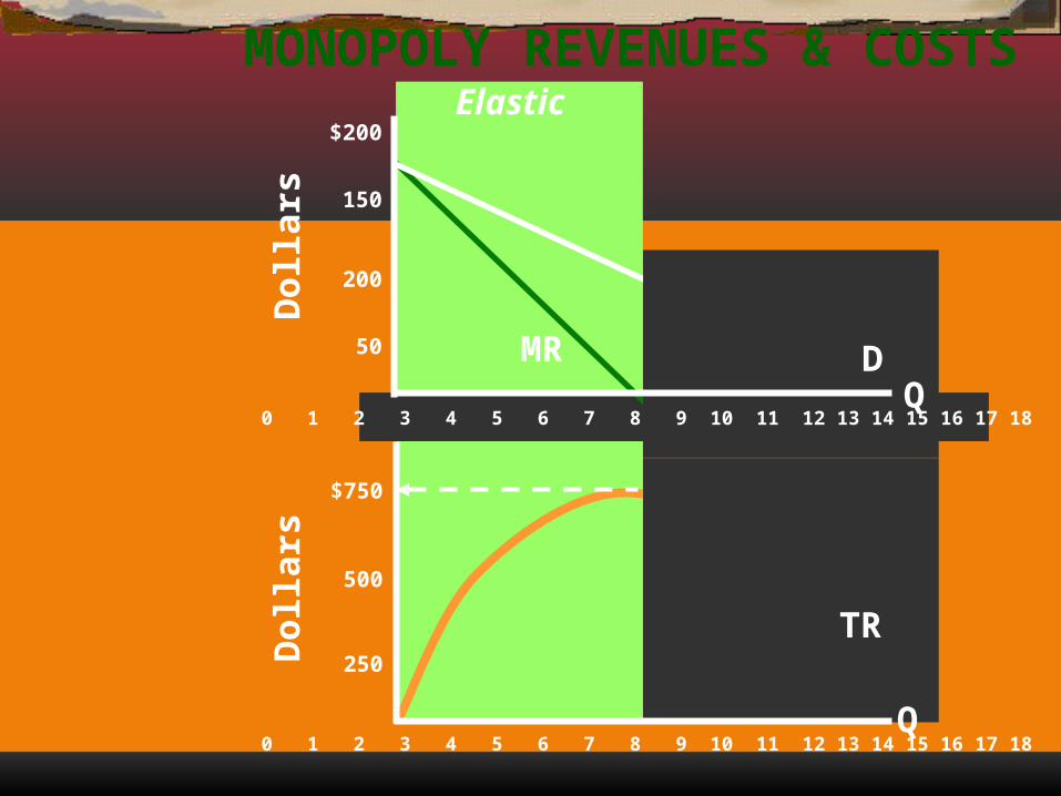
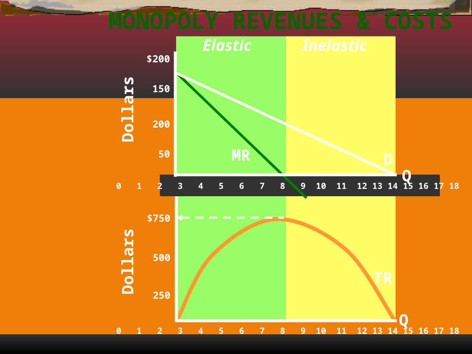
Price and Marginal Revenue for a

Monopoly

Price and Marginal Revenue for a

Monopoly

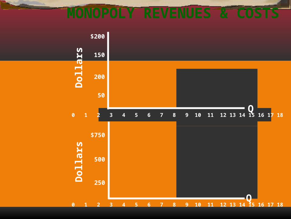
MONOPOLY REVENUES & COSTS

Do

llar

sD

oll

ars

$200

150

200

50

$750

500

250

0 1 2 3 4 5 6 7 8 9 10 11 12 13 14 15 16 17 18

Q0 1 2 3 4 5 6 7 8 9 10 11 12 13 14 15 16 17 18

Q

MONOPOLY REVENUES & COSTS

Do

llar

sD

oll

ars

$200

150

200

50

$750

500

250

MR

Elastic

0 1 2 3 4 5 6 7 8 9 10 11 12 13 14 15 16 17 18

DQ

0 1 2 3 4 5 6 7 8 9 10 11 12 13 14 15 16 17 18

TR

Q

MONOPOLY REVENUES & COSTS

Q

Do

llar

sD

oll

ars

$200

150

200

50

$750

500

250

TR

MR D

InelasticElastic

0 1 2 3 4 5 6 7 8 9 10 11 12 13 14 15 16 17 18Q

0 1 2 3 4 5 6 7 8 9 10 11 12 13 14 15 16 17 18

Failing to remember how to shade the area of ECONOMIC PROFIT

THE PROFIT-MAXIMIZING

POSITION OF A MONOPOLY

Failing to remember how to shade the area of ECONOMIC PROFIT

THE PROFIT-MAXIMIZING

POSITION OF A MONOPOLY

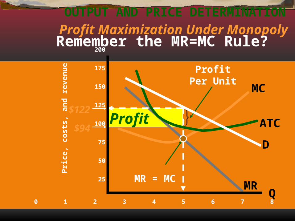
Profit Maximization Under Monopoly

D

MC

ATC

MR

$94

$122Profit

MR = MC

ProfitPer Unit

OUTPUT AND PRICE DETERMINATION

Q

200

175

150

125

100

75

50

25

0 1 2 3 4 5 6 7 8 9 10

Pri

ce,

cost

s, a

nd

rev

enu

e

Remember the MR=MC Rule?

And the Shading of Economic Losses

LOSS MINIMIZATION OF THE IMPERFECT

COMPETITOR

And the Shading of Economic Losses

LOSS MINIMIZATION OF THE IMPERFECT

COMPETITOR

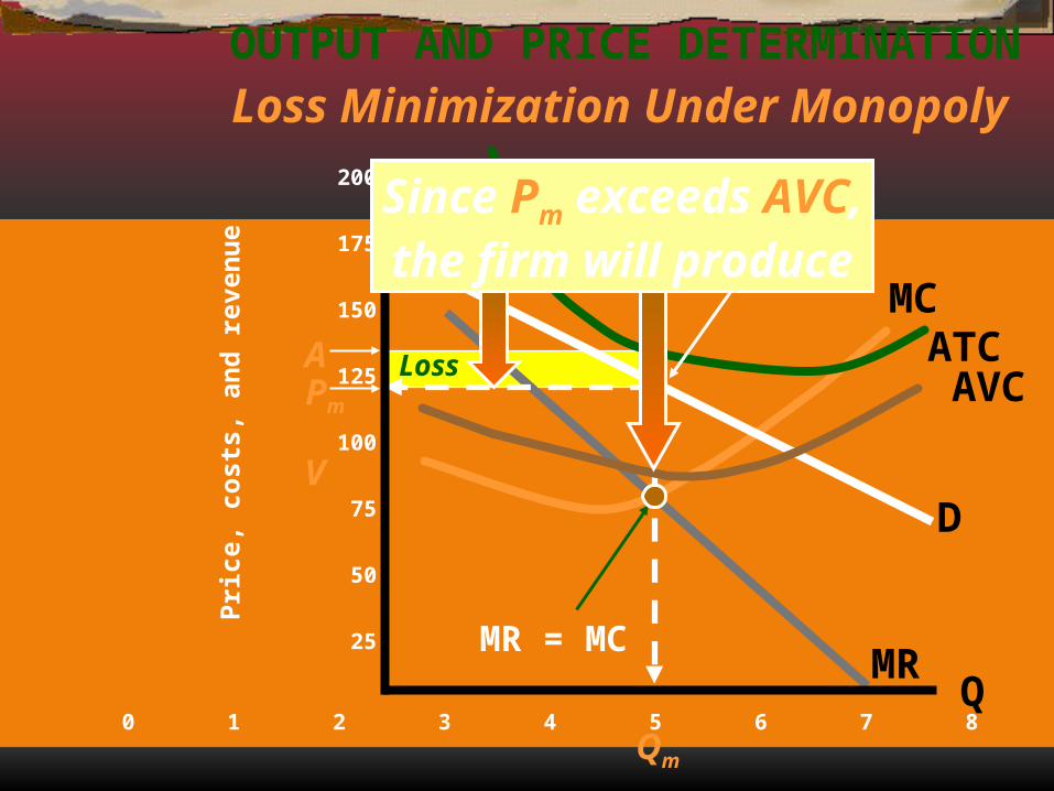
Loss Minimization Under Monopoly

D

MCATC

MR

APm

Loss

MR = MC

LossPer Unit

OUTPUT AND PRICE DETERMINATION

Q

200

175

150

125

100

75

50

25

0 1 2 3 4 5 6 7 8 9 10

Pri

ce,

cost

s, a

nd

rev

enu

e

AVC

Qm

V

Since Pm exceeds AVC,the firm will produce

Monopoly

vs.

Competition

Monopoly

vs.

Competition

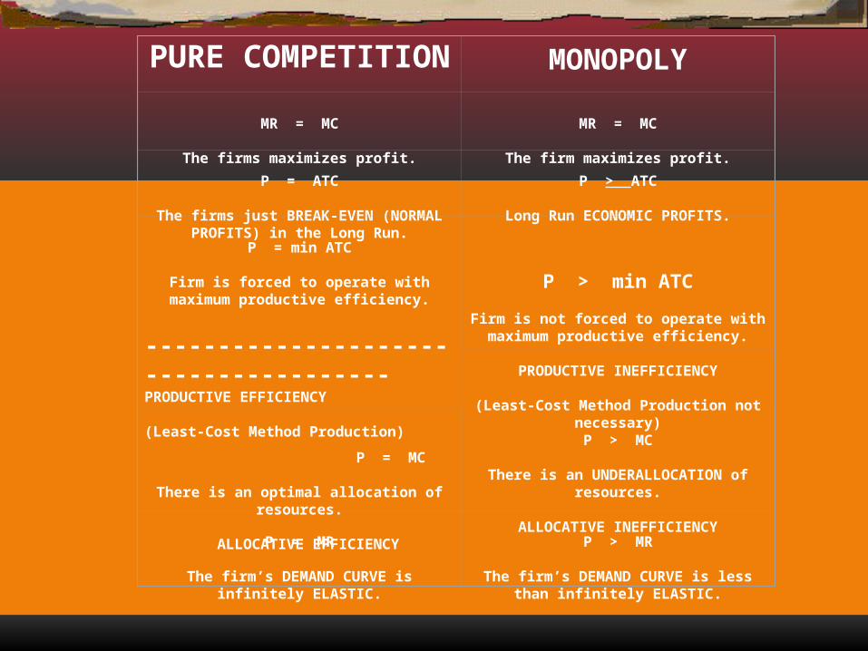
PURE COMPETITION

MONOPOLY

MR = MC

The firms maximizes profit.

MR = MC

The firm maximizes profit.

P = ATC

The firms just BREAK-EVEN (NORMAL PROFITS) in the Long Run.

P > ATC

Long Run ECONOMIC PROFITS.

P = min ATC

Firm is forced to operate with maximum productive

efficiency.

 --------------------------------------PRODUCTIVE EFFICIENCY (Least-Cost Method Production)

 

P > min ATC 

Firm is not forced to operate with maximum productive efficiency.

PRODUCTIVE INEFFICIENCY

(Least-Cost Method Production not necessary)

P = MC

There is an optimal allocation of resources.

ALLOCATIVE EFFICIENCY

P > MC

There is an UNDERALLOCATION of resources.

ALLOCATIVE INEFFICIENCY

P = MR

The firm’s DEMAND CURVE is infinitely ELASTIC.

P > MR

The firm’s DEMAND CURVE is less than infinitely

ELASTIC.

Q

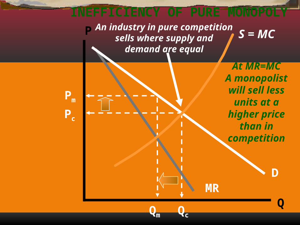
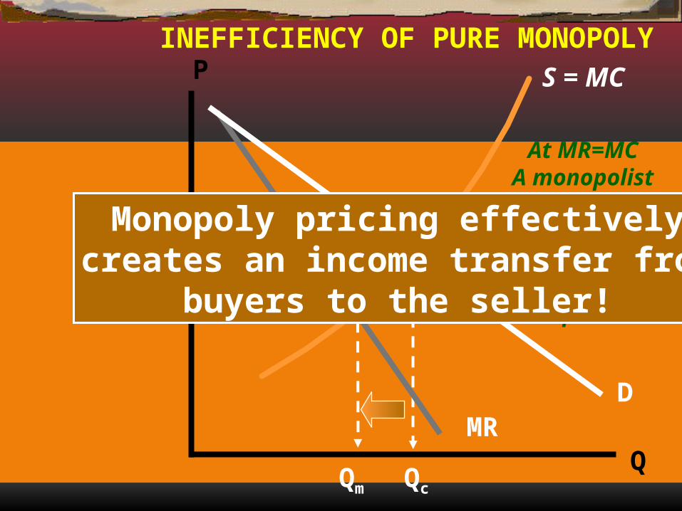
INEFFICIENCY OF PURE MONOPOLY

P

DMR

S = MC

Pc

Pm

QcQm

At MR=MCA monopolistwill sell less

units at ahigher price

than incompetition

An industry in pure competitionsells where supply and

demand are equal

Q

INEFFICIENCY OF PURE MONOPOLYP

DMR

S = MC

Pc

Pm

QcQm

At MR=MCA monopolistwill sell less

units at ahigher price

than incompetition

Monopoly pricing effectivelycreates an income transfer from

buyers to the seller!

Not being able to GRAPH a Natural

Monopoly and the Socially- Optimal

Outputand

Fair-Return Output Levels

Not being able to GRAPH a Natural

Monopoly and the Socially- Optimal

Outputand

Fair-Return Output Levels

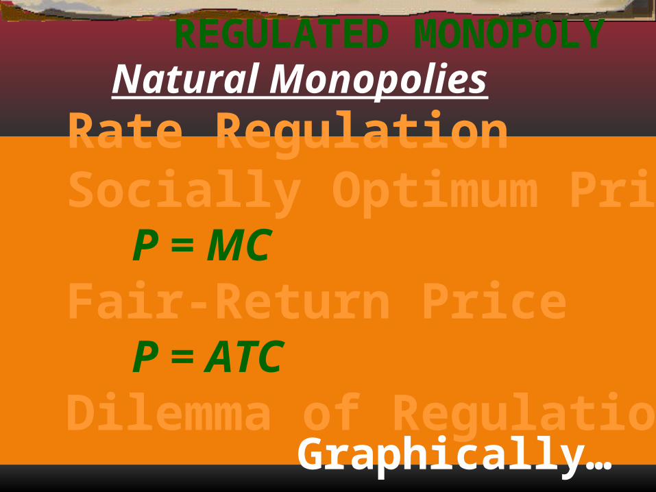
Natural MonopoliesRate RegulationSocially Optimum Price

P = MCFair-Return Price

P = ATCDilemma of Regulation

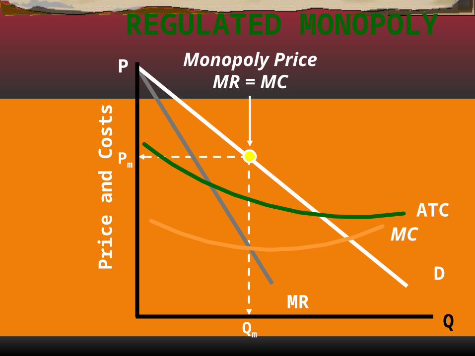
REGULATED MONOPOLY

Graphically…

REGULATED MONOPOLY

Q

D

MR

MCATC

P

Pri

ce a

nd

Co

sts

Monopoly PriceMR = MC

Qm

Pm

REGULATED MONOPOLY

Q

D

MR

MCATC

P

Pri

ce a

nd

Co

sts

Monopoly PriceMR = MC

Qm

Pm

REGULATED MONOPOLY

Q

D

MR

MCATC

P

Pri

ce a

nd

Co

sts

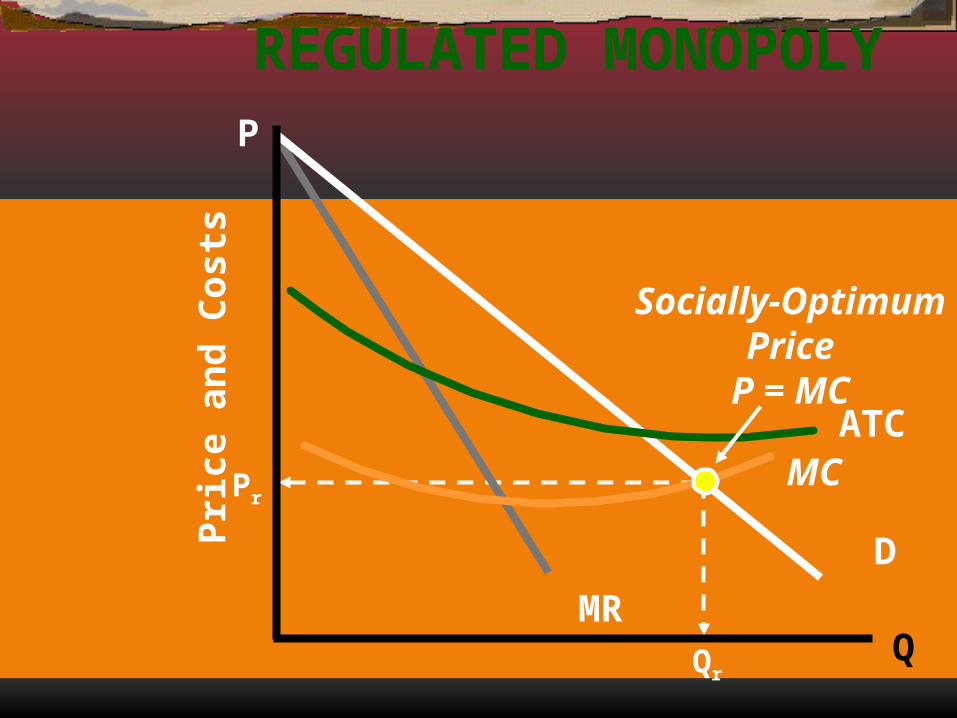
Socially-OptimumPrice

P = MC

Qr

Pr

REGULATED MONOPOLY

Q

D

MR

MCATC

P

Pri

ce a

nd

Co

sts

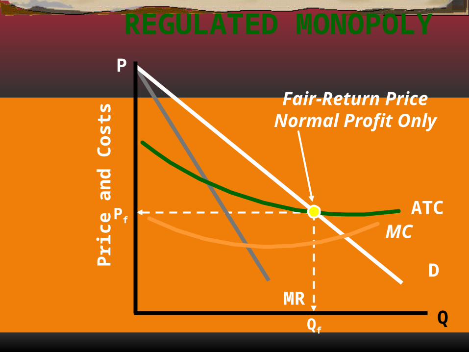
Fair-Return PriceNormal Profit Only

Qf

Pf

REGULATED MONOPOLY

Q

D

MR

MCATC

P

Pri

ce a

nd

Co

sts

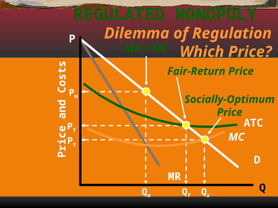
MR = MC

Fair-Return Price

Socially-OptimumPrice

Qm Qf Qr

Dilemma of RegulationWhich Price?

Pm

Pf

Pr

Single PRICE Monopoly

vs.

Price Discrimination

Single PRICE Monopoly

vs.

Price Discrimination

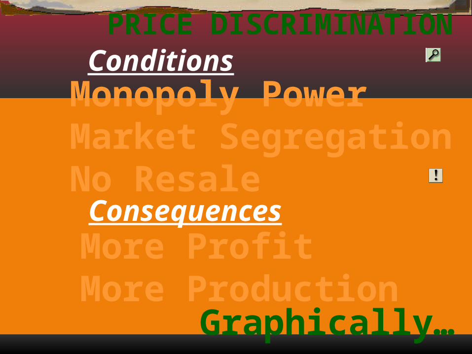
ConditionsMonopoly PowerMarket SegregationNo Resale

ConsequencesMore ProfitMore Production

PRICE DISCRIMINATION

Graphically…

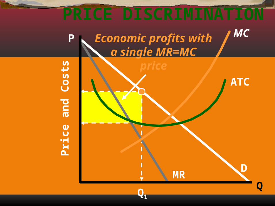
Q

DMR

MC

ATC

P

Q1

Pri

ce a

nd

Co

sts

Economic profits witha single MR=MC

price

PRICE DISCRIMINATION

Q

D

MC

ATC

P

Q1

Pri

ce a

nd

Co

sts

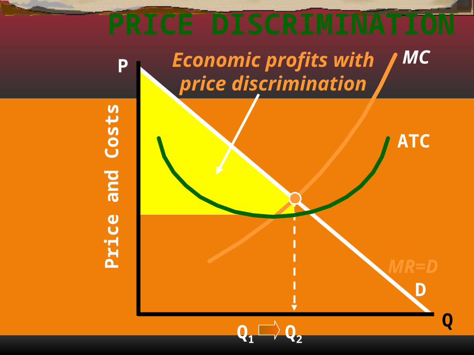
PRICE DISCRIMINATION

Q2

A perfectly discriminatingmonopolist has MR=D,producing more product

and more profit!

MR=D

Q

D

MC

ATC

P

Q1

Pri

ce a

nd

Co

sts

Economic profits withprice discrimination

PRICE DISCRIMINATION

Q2

MR=D

Monopolistic Competiton

What is it?Monopoly?

Competition?

Monopolistic Competiton

What is it?Monopoly?

Competition?

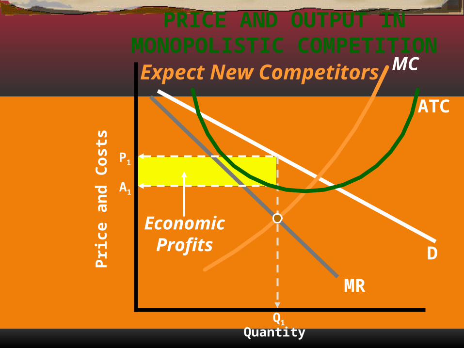
D

MR

P1

ATCP

rice

an

d C

ost

s

Q1

EconomicProfits

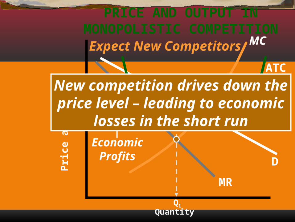
Expect New Competitors

PRICE AND OUTPUT INMONOPOLISTIC COMPETITION

Quantity

A1

MC

D

MR

P1

ATCP

rice

an

d C

ost

s

Q1

EconomicProfits

Expect New Competitors

PRICE AND OUTPUT INMONOPOLISTIC COMPETITION

Quantity

A1

New competition drives down theprice level – leading to economic

losses in the short run

MC

D

MR

MC

P2

ATCP

rice

an

d C

ost

s

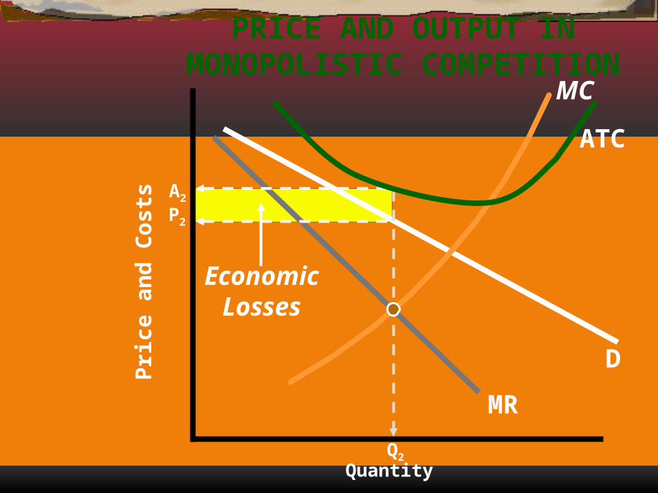
Q2

EconomicLosses

PRICE AND OUTPUT INMONOPOLISTIC COMPETITION

Quantity

A2

D

MR

MC

P2

ATCP

rice

an

d C

ost

s

Q2

EconomicLosses

PRICE AND OUTPUT INMONOPOLISTIC COMPETITION

Quantity

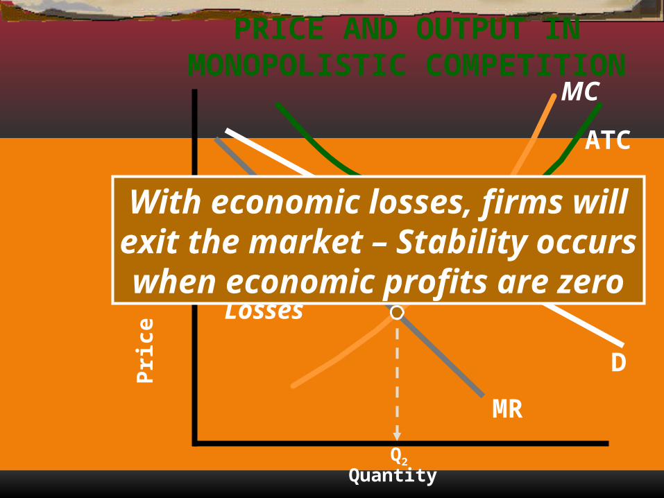
A2With economic losses, firms willexit the market – Stability occurswhen economic profits are zero

D

MR

MC

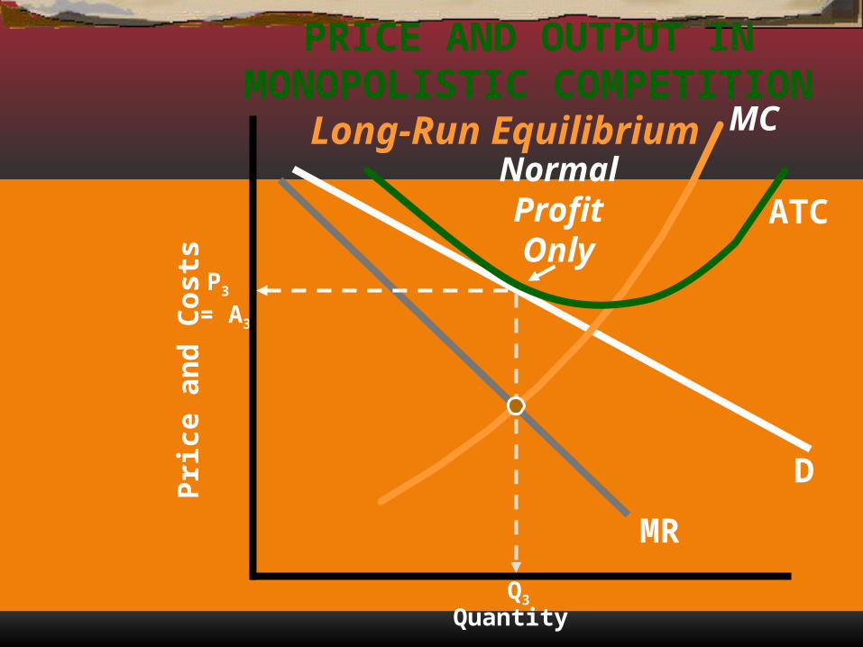
P3 = A3

ATCP

rice

an

d C

ost

s

Q3

PRICE AND OUTPUT INMONOPOLISTIC COMPETITION

Quantity

Long-Run EquilibriumNormalProfitOnly

NOW,

for theRESOURCE (Factor)

MARKETS

NOW,

for theRESOURCE (Factor)

MARKETS

Remember…

Product Market:

MR = MC

Resource Market:

MRP = MFC

Remember…

Product Market:

MR = MC

Resource Market:

MRP = MFC

Units ofResource

TotalProduct(Output)

Marginalproduct

(MP)Product

PriceTotal

Revenue

MarginalRevenue

Product (MRP)

]]]]]]

0 1 2 3 4 5 6 7 8 Q

P 141210 8 6 4 2R

esou

rce

pric

e(w

age

rate

)

Quantity of resource demanded

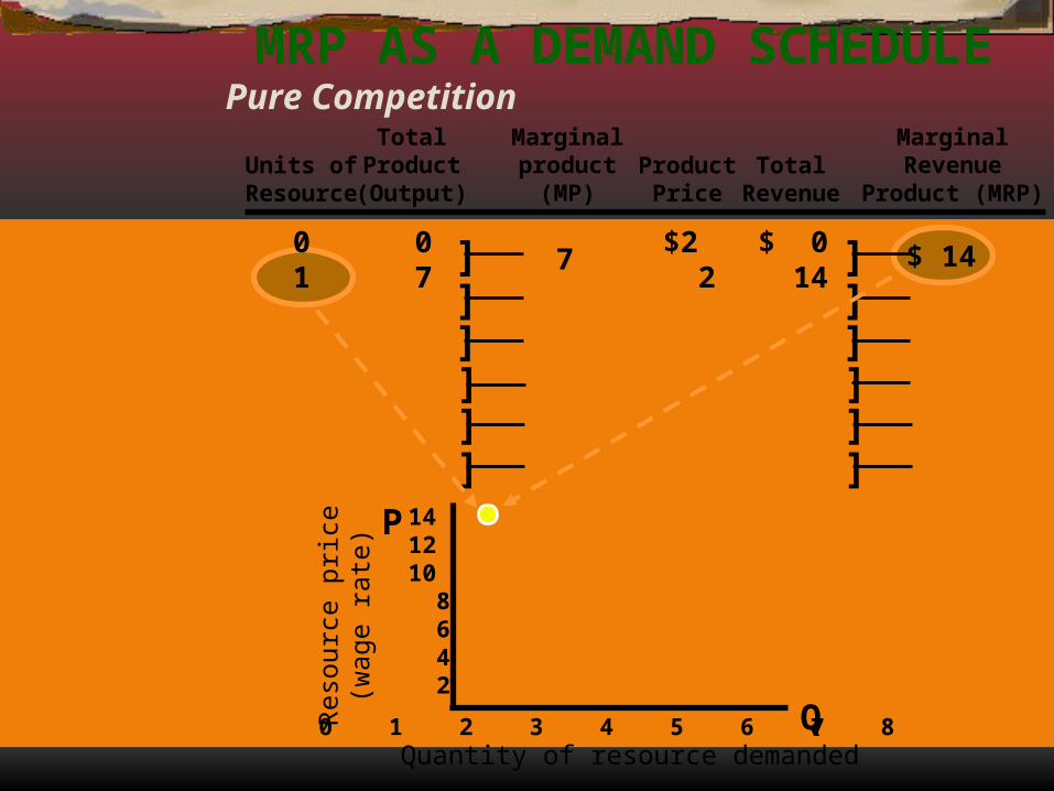
Pure CompetitionMRP AS A DEMAND SCHEDULE

]]]]]]

01

0 7

7$2 2

$ 0 14

$ 14

Units ofResource

TotalProduct(Output)

Marginalproduct

(MP)Product

PriceTotal

Revenue

MarginalRevenue

Product (MRP)

]]]]]]

0 1 2 3 4 5 6 7 8 Q

P 141210 8 6 4 2R

esou

rce

pric

e(w

age

rate

)

Quantity of resource demanded

Pure CompetitionMRP AS A DEMAND SCHEDULE

]]]]]]

012

0 713

76

$2 2 2

$ 0 14 26

$ 14 12

Units ofResource

TotalProduct(Output)

Marginalproduct

(MP)Product

PriceTotal

Revenue

MarginalRevenue

Product (MRP)

]]]]]]

0 1 2 3 4 5 6 7 8 Q

P 141210 8 6 4 2R

esou

rce

pric

e(w

age

rate

)

Quantity of resource demanded

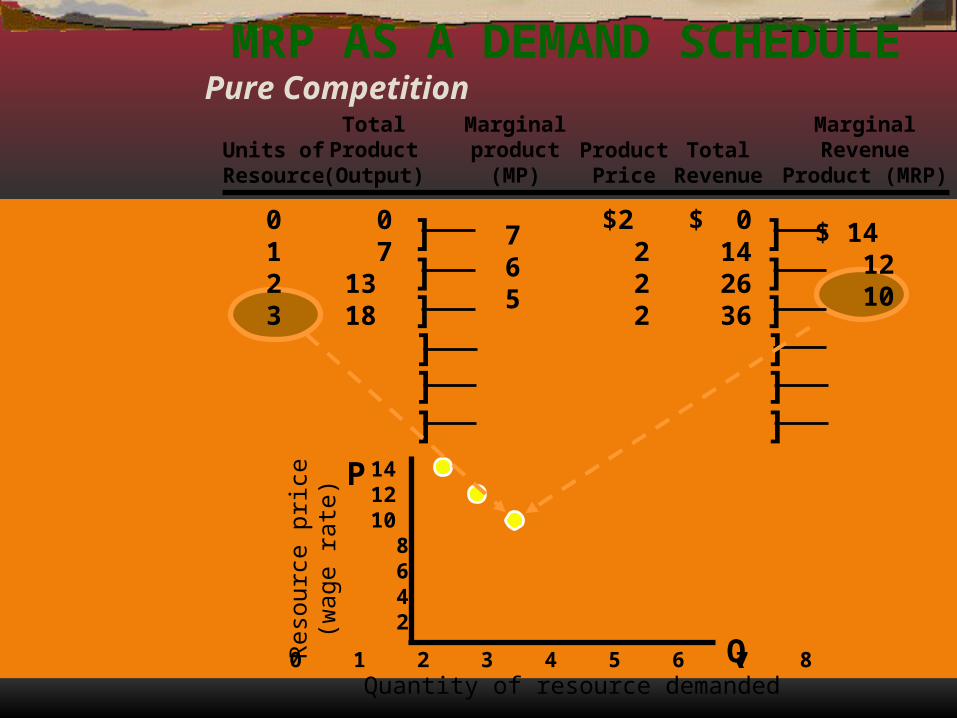
Pure CompetitionMRP AS A DEMAND SCHEDULE

]]]]]]

0123

0 71318

765

$2 2 2 2

$ 0 14 26 36

$ 14 12 10

Units ofResource

TotalProduct(Output)

Marginalproduct

(MP)Product

PriceTotal

Revenue

MarginalRevenue

Product (MRP)

]]]]]]

0 1 2 3 4 5 6 7 8 Q

P 141210 8 6 4 2R

esou

rce

pric

e(w

age

rate

)

Quantity of resource demanded

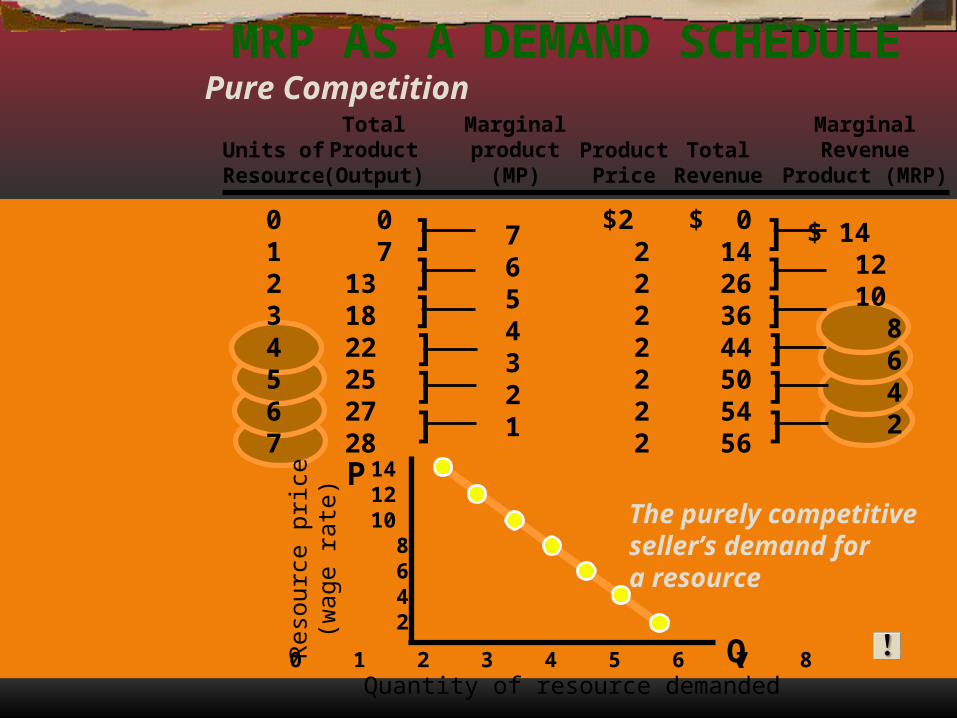
Pure CompetitionMRP AS A DEMAND SCHEDULE

]]]]]]

01234567

0 7131822252728

7654321

$2 2 2 2 2 2 2 2

$ 0 14 26 36 44 50 54 56

$ 14 12 10 8 6 4 2

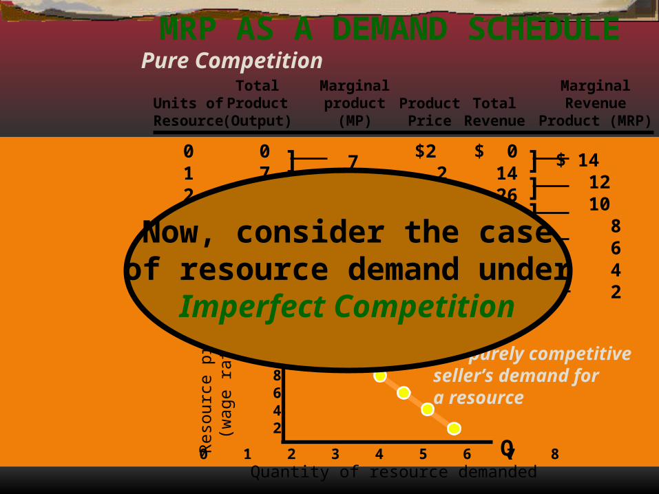
The purely competitiveseller’s demand fora resource

Units ofResource

TotalProduct(Output)

Marginalproduct

(MP)Product

PriceTotal

Revenue

MarginalRevenue

Product (MRP)

]]]]]]

0 1 2 3 4 5 6 7 8 Q

P 141210 8 6 4 2R

esou

rce

pric

e(w

age

rate

)

Quantity of resource demanded

Pure CompetitionMRP AS A DEMAND SCHEDULE

]]]]]]

01234567

0 7131822252728

7654321

$2 2 2 2 2 2 2 2

$ 0 14 26 36 44 50 54 56

$ 14 12 10 8 6 4 2

The purely competitiveseller’s demand fora resource

Now, consider the caseof resource demand under

Imperfect Competition

Units ofResource

TotalProduct(Output)

Marginalproduct

(MP)Product

PriceTotal

Revenue

MarginalRevenue

Product (MRP)

]]]]]]

0 1 2 3 4 5 6 7 8 Q

P 141210 8 6 4 2R

esou

rce

pric

e(w

age

rate

)

Quantity of resource demanded

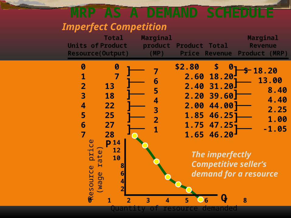
Imperfect CompetitionMRP AS A DEMAND SCHEDULE

]]]]]]

01234567

0 7131822252728

7654321

$2.80 2.60 2.40 2.20 2.00 1.85 1.75 1.65

$ 0 18.20 31.20 39.60 44.00 46.25 47.25 46.20

$ 18.20 13.00 8.40 4.40 2.25 1.00 -1.05

The imperfectlyCompetitive seller’sdemand for a resource

LABOR MARKETS:

Wage Determination

LABOR MARKETS:

Wage Determination

PURELY COMPETITIVELABOR MARKET

Purely competitive labor market:

Many Firms

Numerous Qualified Workers

“Wage Taker” Behavior

Market Demand for Labor

Market Supply of Labor

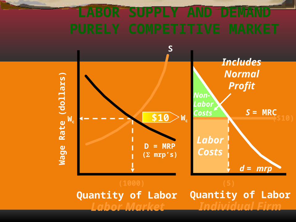
Non-LaborCosts

LaborCosts

LABOR SUPPLY AND DEMANDPURELY COMPETITIVE MARKET

Labor Market

S

D = MRP( mrp’s)

Wc

(1000)

Individual Firm

S = MRC

d = mrp

Wc

Quantity of Labor

Wa

ge

Ra

te (

do

llars

)

Quantity of Labor

($10)

(5)

$10 $10 $10 $10 $10 $10

IncludesNormalProfit

Wa

ge

Ra

te (

do

llars

)S

Quantity of Labor

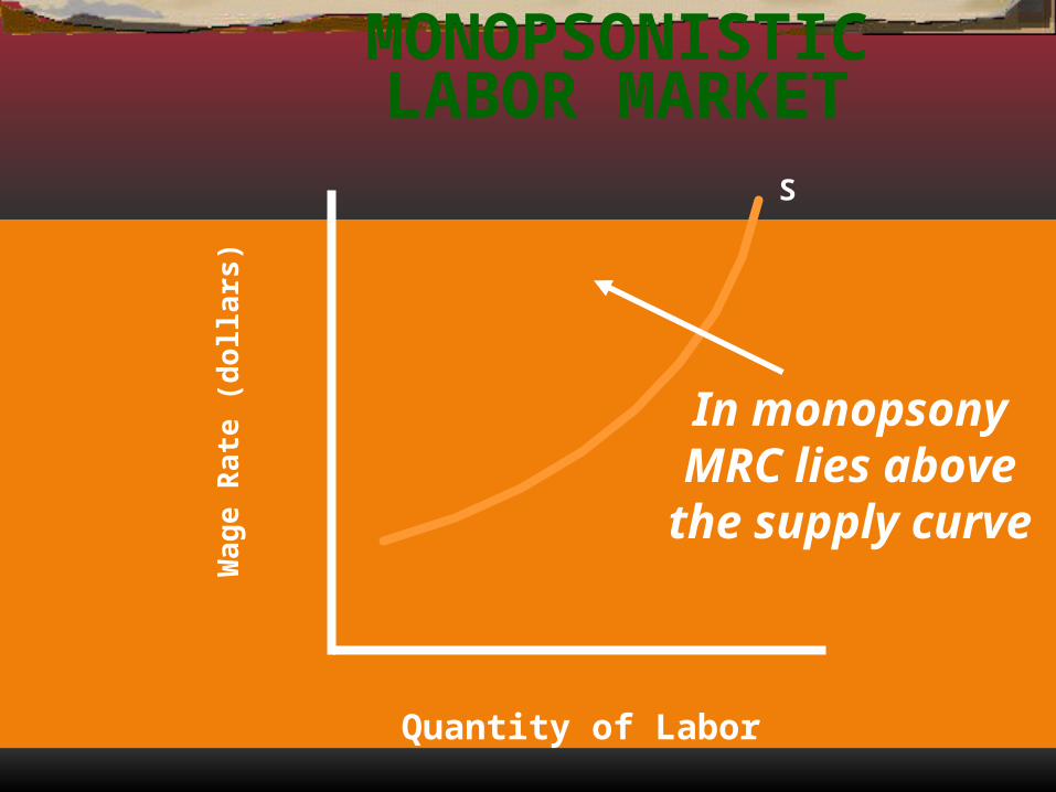
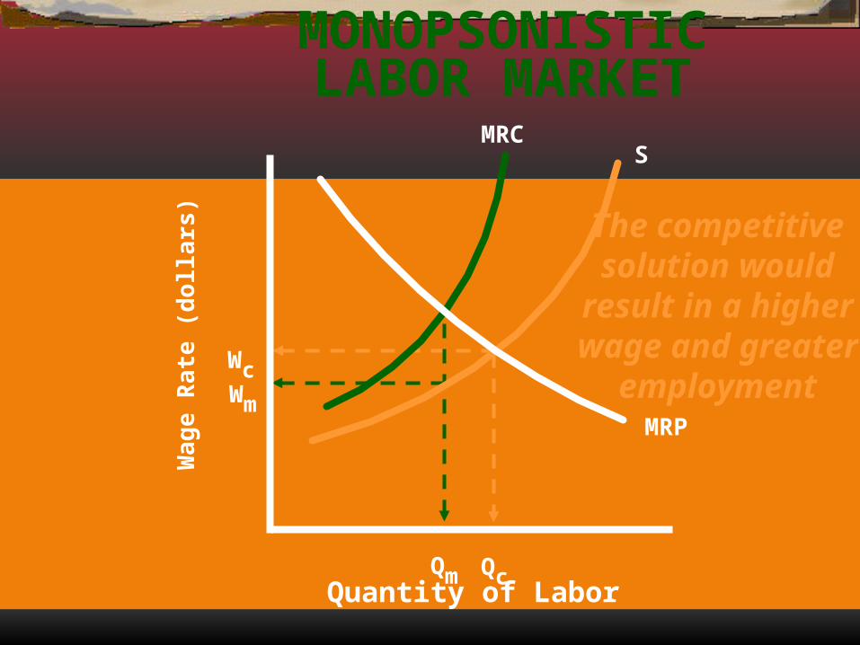
MONOPSONISTICLABOR MARKET

In monopsonyMRC lies abovethe supply curve

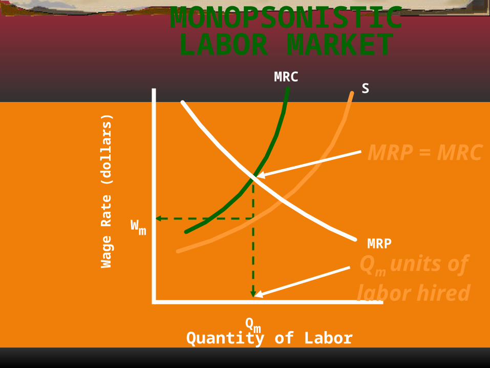
Wa

ge

Ra

te (

do

llars

)

MRP

S

Wm

Quantity of Labor

MRC

Qm

MONOPSONISTICLABOR MARKET

MRP = MRC

Qm units oflabor hired

Wa

ge

Ra

te (

do

llars

)

MRP

S

Wm

Quantity of Labor

MRC

Wc

Qm Qc

The competitivesolution would

result in a higherwage and greater

employment

MONOPSONISTICLABOR MARKET

EXTERNALITIES

Negative

Positive

EXTERNALITIES

Negative

Positive

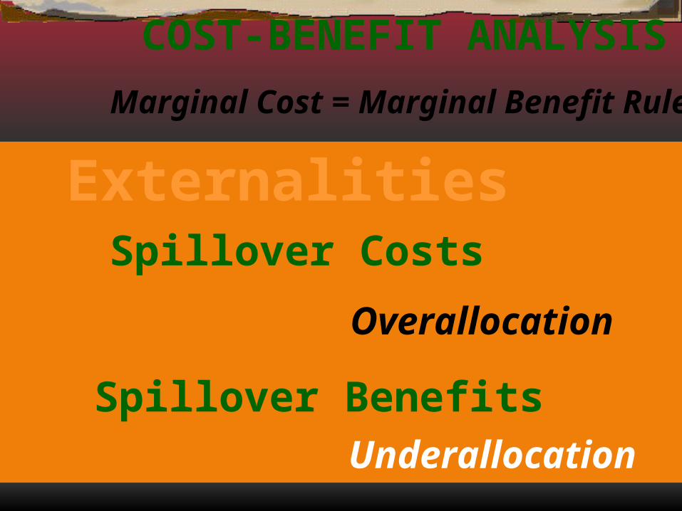
COST-BENEFIT ANALYSIS

Marginal Cost = Marginal Benefit Rule

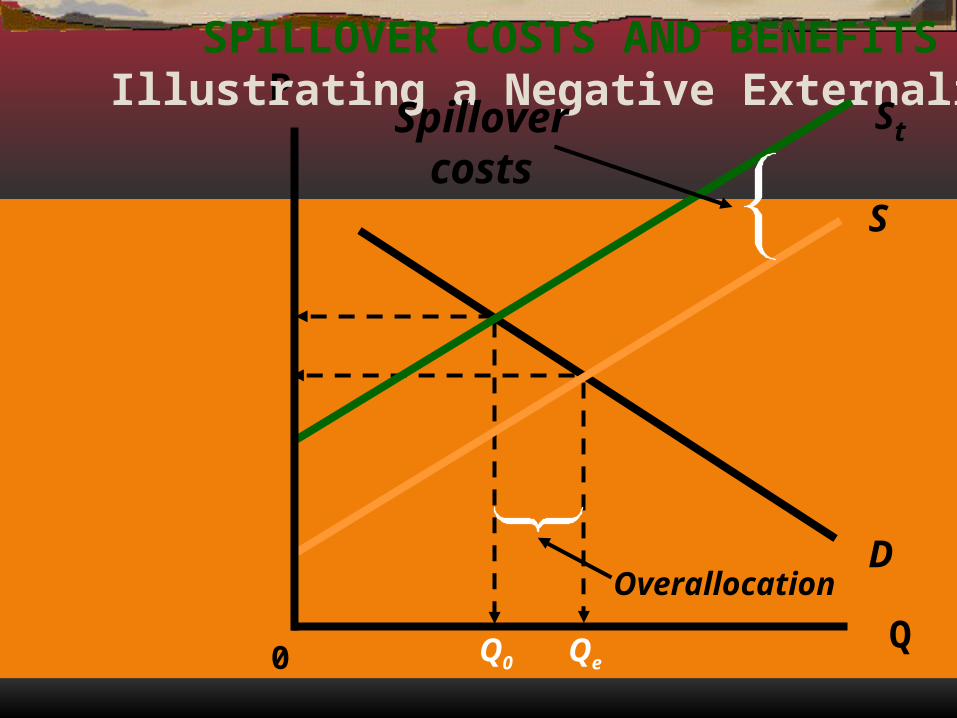
Spillover Costs

Overallocation

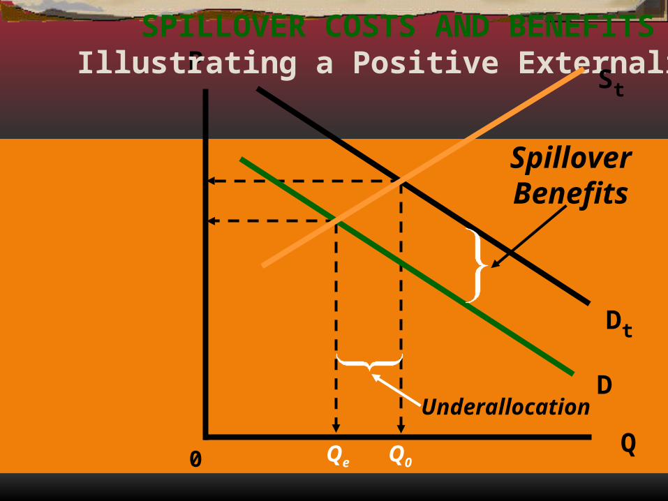
Spillover BenefitsUnderallocation

Externalities

P

Q

SPILLOVER COSTS AND BENEFITSIllustrating a Negative Externality

D

0

Spillovercosts

St

S

Overallocation

Q0 Qe

P

Q

SPILLOVER COSTS AND BENEFITSIllustrating a Positive Externality

0 Qe Q0

D

Dt

SpilloverBenefits

St

Underallocation

Taxation ConceptsTaxation Concepts

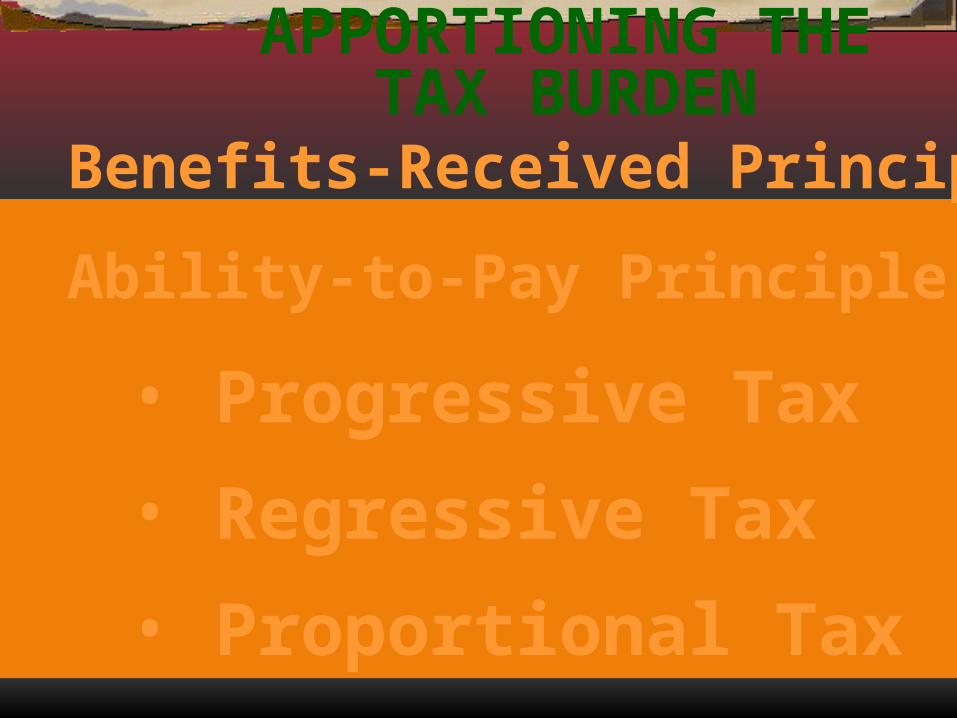
APPORTIONING THE

TAX BURDENBenefits-Received Principle

Ability-to-Pay Principle

• Progressive Tax

• Regressive Tax

• Proportional Tax

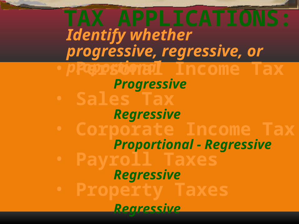
TAX APPLICATIONS:

• Personal Income TaxProgressive

• Sales TaxRegressive

• Corporate Income TaxProportional - Regressive

• Payroll TaxesRegressive

• Property TaxesRegressive

Identify whether progressive, regressive, or proportional

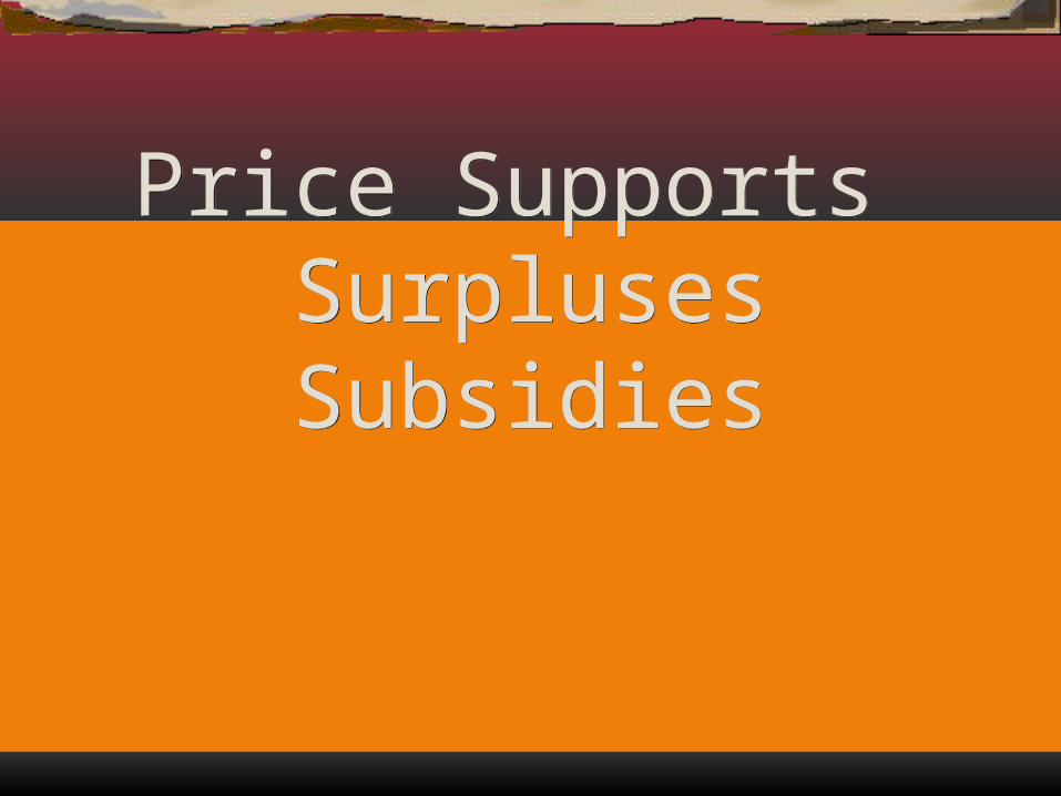
Price Supports SurplusesSubsidies

Price Supports SurplusesSubsidies

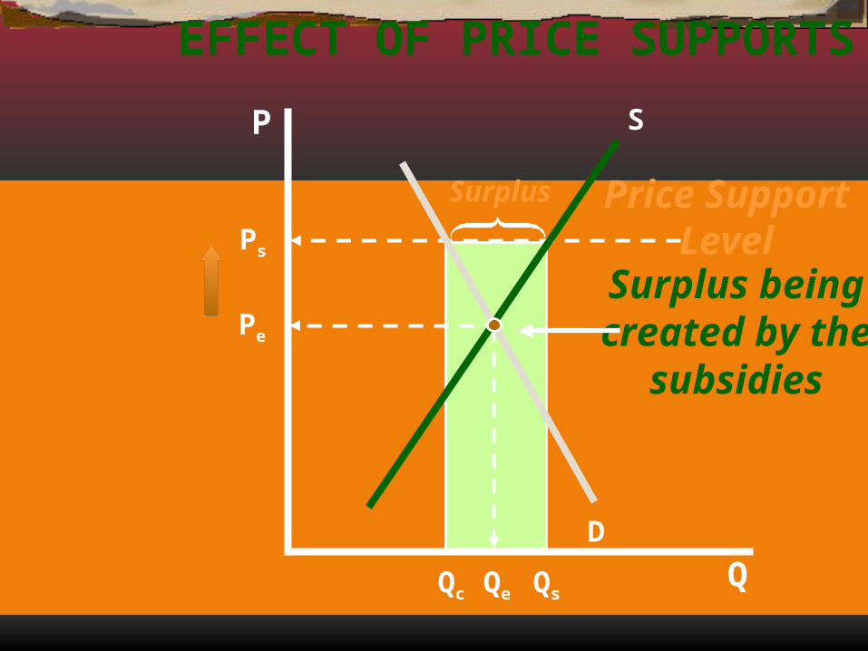
EFFECT OF PRICE SUPPORTS

Pe

D

S

QeQc Qs

Surplus

Ps

Surplus beingcreated by thesubsidies

Q

P

Price SupportLevel

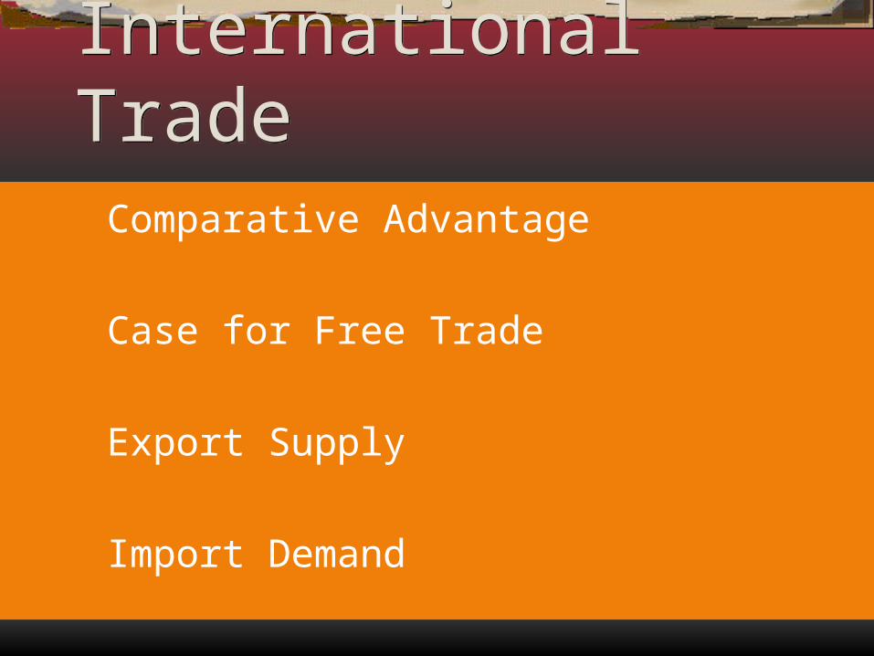
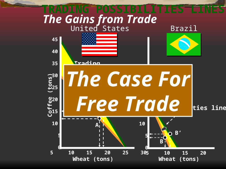
International TradeInternational Trade Comparative Advantage

Case for Free Trade

Export Supply

Import Demand

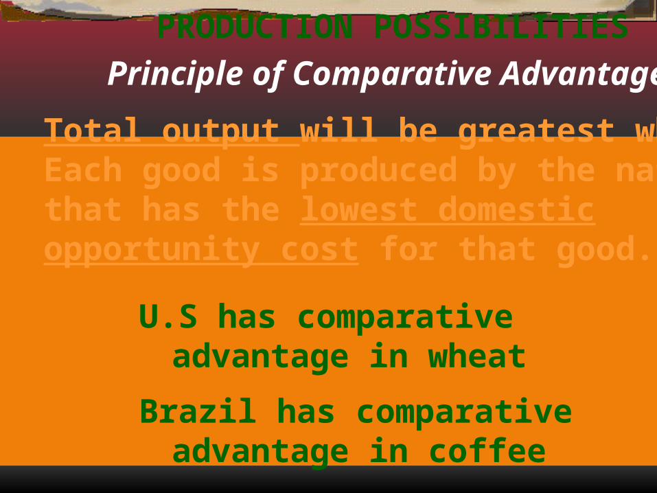
Total output will be greatest whenEach good is produced by the nationthat has the lowest domesticopportunity cost for that good.

U.S has comparative advantage in wheat

Brazil has comparative advantage in coffee

Principle of Comparative Advantage

PRODUCTION POSSIBILITIES

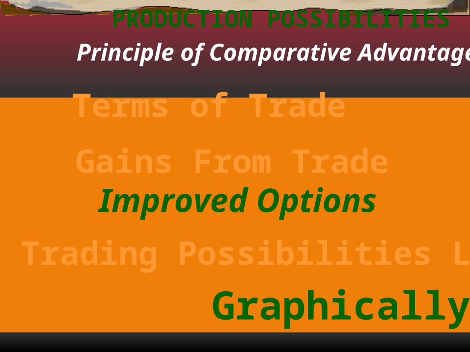
Terms of Trade

Gains From TradeImproved Options

Principle of Comparative Advantage

PRODUCTION POSSIBILITIES

Trading Possibilities Line

Graphically…

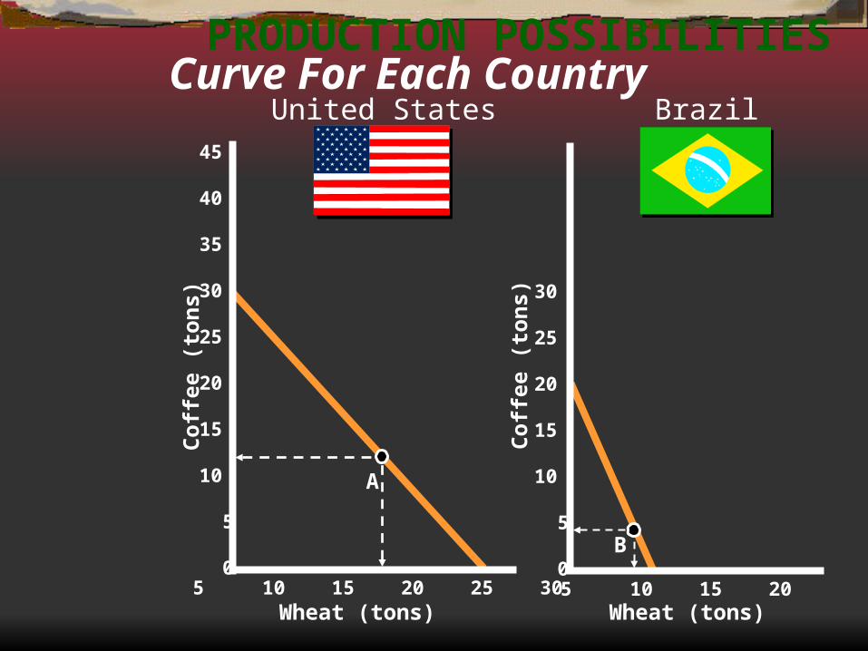
PRODUCTION POSSIBILITIES

A

B

Co

ffee

(to

ns)

Co

ffee

(to

ns)

45

40

35

30

25

20

15

10

5

0

30

25

20

15 10 5

05 10 15 20 25 30 5 10 15 20

Wheat (tons) Wheat (tons)

Curve For Each CountryUnited States Brazil

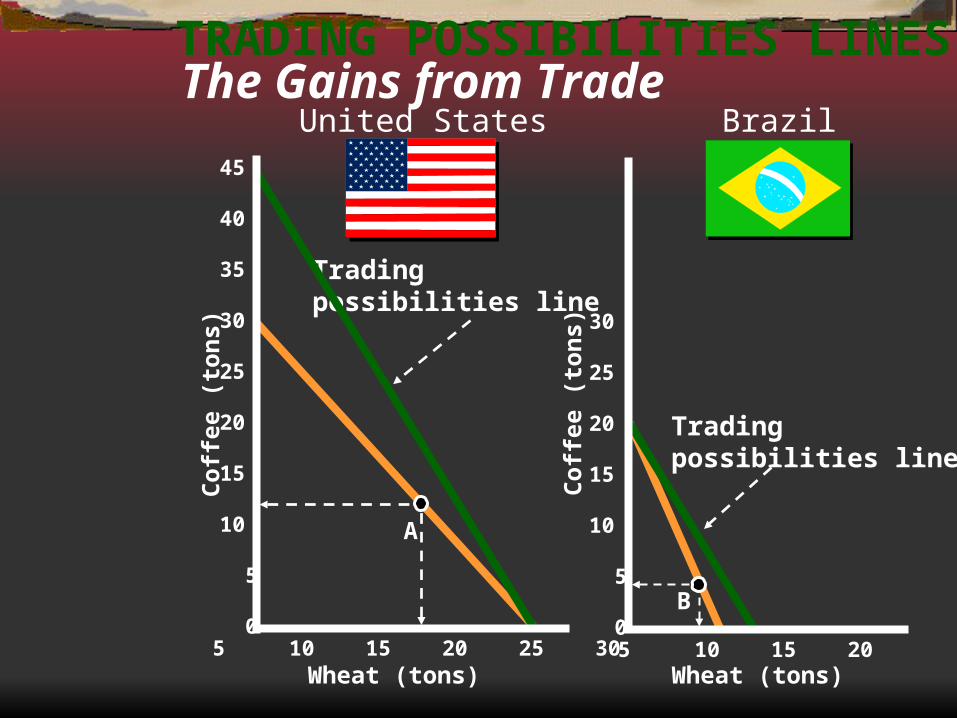
TRADING POSSIBILITIES LINES

Co

ffee

(to

ns)

Co

ffee

(to

ns)

45

40

35

30

25

20

15

10

5

0

30

25

20

15 10 5

05 10 15 20 25 30 5 10 15 20

A

B

Tradingpossibilities line

Tradingpossibilities line

Wheat (tons) Wheat (tons)

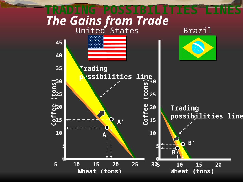
The Gains from TradeUnited States Brazil

TRADING POSSIBILITIES LINES

Co

ffee

(to

ns)

Co

ffee

(to

ns)

45

40

35

30

25

20

15

10

5

0

30

25

20

15 10 5

05 10 15 20 25 30 5 10 15 20

A

B

Tradingpossibilities line

Tradingpossibilities line

A’

B’

Wheat (tons) Wheat (tons)

The Gains from TradeUnited States Brazil

TRADING POSSIBILITIES LINES

Co

ffee

(to

ns)

Co

ffee

(to

ns)

45

40

35

30

25

20

15

10

5

0

30

25

20

15 10 5

05 10 15 20 25 30 5 10 15 20

A

B

Tradingpossibilities line

Tradingpossibilities line

A’

B’

Wheat (tons) Wheat (tons)

The Gains from TradeUnited States Brazil

The Case ForFree Trade

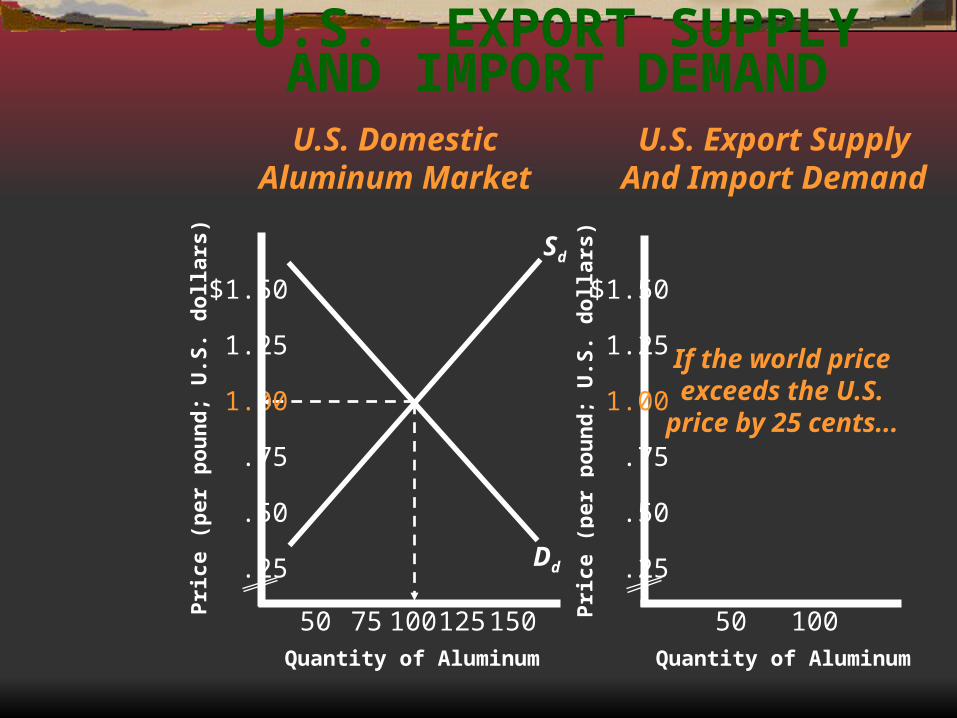
U.S. EXPORT SUPPLYAND IMPORT DEMAND

U.S. DomesticAluminum Market

U.S. Export SupplyAnd Import Demand

Dd

Sd

If the world priceexceeds the U.S.

price by 25 cents...

$1.50

1.25

1.00

.75

.50

.25Pri

ce (

per

po

un

d;

U.S

. do

llars

)

10050 75 125150Quantity of Aluminum

10050P

rice

(p

er p

ou

nd

; U

.S. d

olla

rs)

$1.50

1.25

1.00

.75

.50

.25

Quantity of Aluminum

EXPORTS = 50

U.S. EXPORT SUPPLYAND IMPORT DEMAND

U.S. DomesticAluminum Market

U.S. Export SupplyAnd Import Demand

$1.50

1.25

1.00

.75

.50

.25

10050

DdPri

ce (

per

po

un

d;

U.S

. do

llars

)

Pri

ce (

per

po

un

d;

U.S

. do

llars

)

10050 75 125150

SURPLUS = 50

$1.50

1.25

1.00

.75

.50

.25

If the world pricegoes further up...

Sd

Quantity of Aluminum Quantity of Aluminum

EXPORTS = 50

EXPORTS = 100

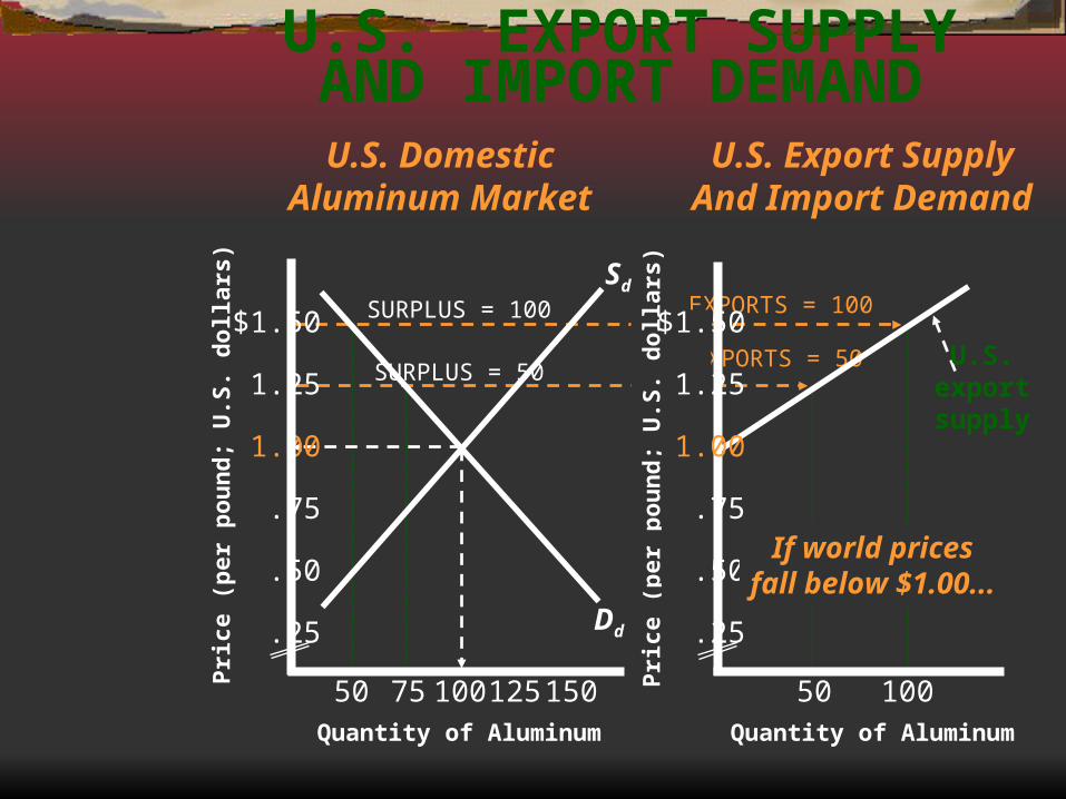
U.S. EXPORT SUPPLYAND IMPORT DEMAND

U.S. DomesticAluminum Market

U.S. Export SupplyAnd Import Demand

$1.50

1.25

1.00

.75

.50

.25

10050

DdPri

ce (

per

po

un

d;

U.S

. do

llars

)

Pri

ce (

per

po

un

d;

U.S

. do

llars

)

10050 75 125150

SURPLUS = 50

SURPLUS = 100 $1.50

1.25

1.00

.75

.50

.25

If world pricesfall below $1.00...

Sd

U.S.exportsupply

Quantity of Aluminum Quantity of Aluminum

SHORTAGE = 50

U.S. EXPORT SUPPLYAND IMPORT DEMAND

U.S. DomesticAluminum Market

U.S. Export SupplyAnd Import Demand

$1.50

1.25

1.00

.75

.50

.25

10050

DdPri

ce (

per

po

un

d;

U.S

. do

llars

)

Pri

ce (

per

po

un

d;

U.S

. do

llars

)

10050 75 125150

SURPLUS = 50

SURPLUS = 100 $1.50

1.25

1.00

.75

.50

.25

Sd

EXPORTS = 50

EXPORTS = 100

IMPORTS = 50

U.S.exportsupply

Quantity of Aluminum Quantity of Aluminum

SHORTAGE = 50

SHORTAGE = 100

U.S. EXPORT SUPPLYAND IMPORT DEMAND

U.S. DomesticAluminum Market

U.S. Export SupplyAnd Import Demand

$1.50

1.25

1.00

.75

.50

.25

10050

DdPri

ce (

per

po

un

d;

U.S

. do

llars

)

Pri

ce (

per

po

un

d;

U.S

. do

llars

)

10050 75 125150

SURPLUS = 50

SURPLUS = 100

U.S.exportsupply

EXPORTS = 50

EXPORTS = 100

IMPORTS = 50

IMPORTS = 100

U.S.import

demand

$1.50

1.25

1.00

.75

.50

.25

Sd

Quantity of Aluminum Quantity of Aluminum

CANADIAN EXPORT SUPPLYAND IMPORT DEMANDCanada’s DomesticAluminum Market

Canada’s Export SupplyAnd Import Demand

DdSHORTAGE = 50

$1.50

1.25

1.00

.75

.50

.25

10050

Pri

ce (

per

po

un

d;

U.S

. do

llars

)

Pri

ce (

per

po

un

d;

U.S

. do

llars

)

10050 75 125150

SURPLUS = 100

Canadianexportsupply

Canadianimport

demand

$1.50

1.25

1.00

.75

.50

.25

Sd

SURPLUS = 50

Quantity of Aluminum Quantity of Aluminum

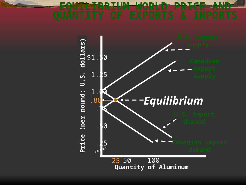
EQUILIBRIUM WORLD PRICE ANDQUANTITY OF EXPORTS & IMPORTS

Pri

ce (

per

po

un

d;

U.S

. d

oll

ars)

U.S. exportsupply

U.S. importdemand

Quantity of Aluminum

Canadianexportsupply

Canadian importdemand

10050

$1.50

1.25

1.00

.75

.50

.25

25

.88 Equilibrium