Economic Modelling 35 (2013) 472–476

Contents lists available at ScienceDirect

Economic Modelling

j ourna l homepage: www.e lsev ie r .com/ locate /ecmod

Common trends and common cycles in stock markets

Paresh Kumar Narayan ⁎, Kannan S. ThuraisamyCentre for Financial Econometrics, School of Accounting, Economics and Finance, Faculty of Business and Law, Deakin University, 221 Burwood Highway, Burwood, Victoria 3125, Australia

⁎ Corresponding author. Tel.: +61 3 9244 6180; fax: +E-mail addresses: paresh.narayan@deakin.edu.au (P.K.

Kannan.thuraisamy@deakin.edu.au (K.S. Thuraisamy).

0264-9993/$ – see front matter © 2013 Elsevier B.V. All rihttp://dx.doi.org/10.1016/j.econmod.2013.08.002

a b s t r a c t

a r t i c l e i n f o

Article history:Accepted 1 August 2013Available online xxxx

JEL classification:C22F31

Keywords:Stock pricesTrend-cycle decompositionPermanent and transitory shocks

In this paper we examine the role of permanent and transitory shocks in explaining variations in the S&P 500,Dow Jones and the NASDAQ. Our modeling technique involves imposing both common trend and commoncycle restrictions in extracting the variance decomposition of shocks. We find that: (1) the three stock price in-dices are characterized by a common trend and common cycle relationship; and (2) permanent shocks explainthe bulk of the variations in stock prices over short horizons.

© 2013 Elsevier B.V. All rights reserved.

1. Introduction

What determines stockmarket volatility is an important topic fromamonetary policymaker's point of view for two reasons. First, havingreliable estimates of the impact of monetary policies on the financialmarkets will be instrumental in formulating effective policy decisions.From the perspective of monetary policymakers, having reliable esti-mates of the reaction of asset prices to policy instruments is a criticalstep in formulating effective policy decisions. Much of the transmissionof monetary policy comes through the influence of short-term interestrates on other asset prices – including longer term interest rates andstock prices – that determine private borrowing costs and changes inwealth, which in turn influence real economic activity (Rigobon andSack, 2004: 1554). Second, reliable information on the reactions ofstock markets to monetary policies is likely to be useful for financialmarket participants in formulating effective investment and risk man-agement decisions.

There are several studies (Bernanke and Kuttner, 2005; Gallagher,1999; Gallagher and Taylor, 2000, 2002a,b; Lee, 1992; Rapach, 2001)that examine the behavior of stockmarkets at high-frequency horizons.The study closest to ours is Narayan (2010), who examines commoncycles and common trends relationship between three countries'(Singapore, Taiwan, and South Korea) stock price indices. He findsmixed results on the relative importance of permanent and transitory

61 3 9244 6034.Narayan),

ghts reserved.

shocks.1 Our approach is the same as Narayan (2010); however, thereis one principal difference. Instead of focusing on country-level stockmarkets, we consider stock exchanges from a single country—UnitedStates. We believe that if permanent and transitory shocks, in particulartheir relative importance is to be judged, it is best examined if a range ofstock exchanges from within a country is considered. This is an impor-tant consideration because shocks, particularly if the shock (regardlessof how a shock is defined) originates from one of the countries thatare part of the sample (model) then the impact of the shock on thatcountry is likely to be more than the other countries in the model.Therefore, a country-level analysis is likely to suffer from this bias. Bycomparison if stock exchanges of a single country are chosen thenshocks originating from that countrywill have the same degree of expo-sure to all stock exchanges. This, as a result, is a more ideal case for un-derstanding the relative importance of shocks. Subsequently, our maincontribution is this.

The goal of this paper is to examine the importance of permanent andtransitory shocks in explaining variations in three American stock priceseries, namely the S&P 500, Dow Jones and NASDAQ using a more effi-cient trend-cycle decomposition technique. Foreshadowing the mainconclusions, we find that S&P 500, Dow Jones and the NASDAQ shareone common trend and two common cycles, and permanent shocks

1 One must not ignore the fact that common trend and common cycles or simply atrend-cycle decomposition of particularly macroeconomic variables, with a growing focuson business cycle, is popular now. The list of studies is large to be cited here but some pa-pers published in this journal that readers may find of interest are Harvey and Mills(2002), Fukuda (2009), Centoni et al. (2007) Caporale (1997), Narayan (2008), andManfredi and Fanti (2004).

0.3

0.4

0.5

0.6

0.7

0.8

0.9

1.0

1986 1988 1990 1992 1994 1996 1998 2000 2002 2004

Cor(RDJ,RNSQ)Cor(RDJ,RSP)Cor(RNSQ,RSP)

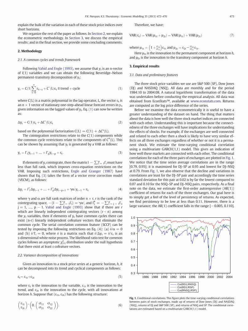
Fig. 1. Conditional correlations. This figure plots the time-varying conditional correlationsbetween pairs of stock exchanges, made up of returns of Dow Jones (DJ) and NASDAQ(NSQ), returns of DJ and S&P 500 (SP), and returns of NSQ and SP. The conditional corre-lations are estimated based on a multivariate GARCH(1,1) model.

473P.K. Narayan, K.S. Thuraisamy / Economic Modelling 35 (2013) 472–476

explain the bulk of the variation in each of these stock price indices overshort horizons.

We organize the rest of the paper as follows. In Section 2, we explainthe econometric methodology. In Section 3, we discuss the empiricalresults; and in thefinal section,we provide some concluding comments.

2. Methodology

2.1. A common cycles and trends framework

Following Vahid and Engle (1993), we assume that yt is an n-vectorof I(1) variables and we can obtain the following Beveridge–Nelsonpermanent-transitory decomposition of yt:

yt ¼ C 1ð ÞX∞s¼0

εt−s þ C� Lð Þεt ≡ trendþ cycle ð1Þ

where C(L) is a matrix polynomial in the lag operator, L, the vector εt isan n × 1 vector of stationary one-step-ahead linear forecast errors in yt,given information on the lagged values of yt. Eq. (1) can now bewrittenas:

Δyt ¼ C 1ð Þεt þ ΔC� Lð Þεt ð2Þ

based on the polynomial factorization C(L) = C(1) + ΔC*(L).The cointegration restrictions relate to the C(1) components while

the common cycle restrictions relate to the components of C⁎(L). Thiscan be shown by assuming that yt is generated by a VAR as follows:

yt ¼ Γ1yt−1 þ…þ Γpyt−p þ εt: ð3Þ

If elements of yt cointegrate, then thematrix I − ∑i = 1p Γi must have

less than full rank, which imposes cross-equation restrictions on theVAR. Imposing such restrictions, Engle and Granger (1987) haveshown that Eq. (3) takes the form of a vector error correction model(VECM), as follows:

Δyt ¼ Γ�1Δyt−1 þ…þ Γ�pΔyt−pþ1 þ γα′yt−1 þ εt ð4Þ

where γ and α are full rank matrices of order n × r, r is the rank of thecointegrating space, −(I − ∑i = 1

p Γi) = γα′, and Γj⁎ = −∑i = j + 1p Γi,

j = 1, …, p − 1. Vahid and Engle (1993) show that if there are rwhich are linearly independent cointegrating vectors (r b n) amongthe yt variables, then if elements of yt have common cycles there canexist (n-r) linearly independent cofeature vectors that eliminate thecommon cycle. The serial correlation common feature (SCCF) can betested by imposing the following restrictions on Eq. (4): (a) δ′α = 0and (b) δ′Γi = 0, where δ is a matrix such that δ′Δyt = δ′εt is ans-dimensionalwhite noise process. The likelihood ratio test for commoncycles follows an asymptotic χ(v)2 distribution under the null hypothesisthat there exist at least s cofeature vectors.

2.2. Variance decomposition of innovations

Given an innovation to a stock price series at a generic horizon, h, itcan be decomposed into its trend and cyclical components as follows:

εt¼ ε1tþε2t ð5Þ

where εt is the innovation to the variable, ε1t is the innovation to thetrend, and ε2t is the innovation to the cycle, with all innovations athorizon h. Suppose that (ε1t, ε2t) has the following structure:

ε1tε2t

� �e 0; σ11 σ12σ21 σ22

� �� �: ð6Þ

Therefore, we have:

VAR εtð Þ ¼ VAR μ1t þ μ2tð Þ ¼ VAR μ1tð Þ þ VAR μ2tð Þ ð7Þ

where μ1t ¼ 1þ σ12σ11

� �ε1t and μ2t ¼ ε2t− σ12

σ11ε1t:

Here μ1t is the innovation to the permanent component at horizon h,and μ2t is the innovation to the transitory component at horizon h.

3. Empirical results

3.1. Data and preliminary features

The three stock price variables we use are S&P 500 (SP), Dow Jones(DJ) and NASDAQ (NSQ). All data are monthly and for the period1984:10 to 2004:08. A natural logarithmic transformation of the datawas undertaken before conducting the empirical analysis. All data wasobtained from EconStats™, available at www.econstats.com. Returnsare computed as the log price difference of the series.

Before we examine the data econometrically it is useful to have agreater understanding of the dataset on hand. The thing that mattersabout the data is howwell the three stockmarket indices are connectedwith each other. Understanding this is important because the connect-edness of the three exchanges will have implications for understandingthe effects of shocks. For example, if the exchanges are well connectedand related to each other then a shock is likely to have very similar ef-fects on all three exchanges regardless of whether or not it is a perma-nent shock. We estimate the time-varying conditional correlationusing a multivariate GARCH(1,1) model. This gives an indication ofhowwell these markets are connected with each other. The conditionalcorrelations for each of the three pairs of exchanges are plotted in Fig. 1.We notice that the time series average correlations are in the range[0.79, 0.95]; it is maximized for DJ–SP at 0.95 and lowest for DJ–NSQat 0.79. From Fig. 1, we also observe that the decline and variations incorrelations are least for the DJ–SP pair and accordingly the time seriesstandard deviation for this pair at 0.02 is by far the lowest compared to0.07 and 0.10 for the NSQ–SP and DJ–NSQ pairs, respectively. As a finalnote on the data, we estimate the first-order autoregressive (AR(1))coefficient of returns for each of the three exchanges. Our goal here isto simply get a feel of the level of persistency of returns. As expected,we find persistency to be low at less than 0.11. However, there is alarge variance; the AR(1) coefficient falls in the range [−0.005, 0.110].

Table 2Narayan and Popp test for unit root in the presence of two endogenous structural breaks.This table reports the results from theNarayan and Popp two endogenous structural breaktest. Themodel includes two structural breaks in the intercept and slope of the time seriesdata (stock price). The structural break dates as reflected in the trend are reportedtogether with the t-test that examines the null hypothesis of a unit root. The optimal laglength used to control for serial correlation is reported in the last row.

S&P 500 Dow Jones NASDAQ

TB1 1989M05 1989M05 1989M05TB2 1993M08 1993M08 1993M08t-Test −0.535 −1.175 −2.474k 2 2 2

Notes: Critical values at the 1%, 5%, and10% are−5.287,−4.692, and−4.396, respectively.Critical values are obtained from Table 3, page 1429 (Narayan and Popp, 2010).

Table 3Cointegration and common feature tests.This table reports three sets of results. In Panel Awe report the trace test for cointegration;in Panel B, we report the maximum eigenvalue test for cointegration; and in Panel C, we

474 P.K. Narayan, K.S. Thuraisamy / Economic Modelling 35 (2013) 472–476

These statistics, taken together, suggest that these three stock ex-changes although of the same country have a fair share of heterogeneity.

3.2. Unit root and cointegration tests

The aim of this section is to examine the integrational properties ofthe S&P 500, Dow Jones andNASDAQ.We achieve this by using two uni-variate tests for unit roots, namely the conventional augmented Dickeyand Fuller (ADF) test and the generalized least squares ADF test, whichexamine the null hypothesis of a unit root againstmean stationarity andtrend stationarity. The results are presented in Table 1. Ourmain findingis as follows. For the log-levels of each of the three stock price variables,using both models with and without a time trend, we are unable to re-ject the unit root null hypothesis at conventional levels of significance.Meanwhile, when we repeat the exercise for the first difference of thestock price series, we are able to reject the unit root null hypothesis,implying that stock prices are either difference stationary or trendstationary. In other words, the ADF test and the ADF-GLS test resultssuggest that the log-levels of stock prices are characterized by a unitroot process.

Perron (1989) argued that if there is a structural break, the power toreject a unit root decreases when the stationary alternative is true andthe structural break is ignored. Narayan and Popp (2013) show thesize and power properties of a range of popular two structural break(endogenous) unit root tests. They consider the Lumsdaine and Papell(1997) test, the Lee and Strazicich (2003) test, and the recently devel-oped Narayan and Popp (2010) test. Their main finding from this com-parison analysis is that the Narayan and Popp two structural break testhas better size and high power and it identifies the structural breaksaccurately. Motivated by these findings, we now consider whethereach of the three stock price indices are unit-root non-stationary usingthe Narayan and Popp test.

The results from the Narayan and Popp test are reported in Table 2.Two results are worth highlighting. First, notice that the two structuralbreak dates are common across all three stock indices. The first breakfollows the 1987US stockmarket crash andprecedes the early 1990s re-cession. The second break follows recessions in the US. This recessionactually lasted from July 1990 toMarch 1991. The secondfinding relatesto the null hypothesis of a unit root. The t-test statistics are reported.These test statistics are all greater than the critical values at the 10%level or better, suggesting that one cannot reject the unit root nullhypothesis. Therefore, we conclude that stock price indices are bestcharacterized by a unit root non-stationary process.

We use Johansen's (1988, 1991) approach, which uses the maxi-mum likelihood procedure to determine the presence of cointegratingvectors among the three stock price series. Johansen and Juselius(1992) recommend the trace test and the maximum eigenvalue teststatistics to determine the number of cointegrating vectors. We use a

Table 1ADF unit root test results.This table reports simple ADF and ADF-GLS tests for testing the null hypothesis of a unitroot. The results are conducted on both levels (logs of stock price) and first difference ofvariables. The models are estimated with and without a time trend. In square bracketswe report the optimal lag length, which is obtained using the Schwarz InformationCriterion (SIC). We begin the lag length selection criteria with a maximum of eight lagsand then implement the SIC procedure.

ADF ADF-GLS

No trend Trend No trend Trend

ln SPtSP −1.6249 [0] −1.4112 [0] 1.3209 [0] −1.2977 [0]Δ ln SPtSP −15.1986 [0] −15.2765 [0] −13.0989 [0] −14.3005 [0]ln SPtDJ −1.5914 [0] −1.8401 [0] 1.5899 [0] −1.5828 [0]Δ ln SPtDJ −15.4138 [0] −15.4814 [0] −13.1619 [0] −14.4625 [0]ln SPtNSDQ −1.3601 [0] −1.5073 [0] 0.6188 [0] −1.5823 [0]Δ ln SPtSP −13.7192 [0] −13.7316 [0] −12.6289 [0] −13.2956 [0]

Notes: The square brackets contain the lag lengths.

model with a restricted intercept but no time trend, and begin the opti-mal lag length searchwith amaximumof 12 lags.We obtain the optimallag length of 8 by using the Schwarz Information Criterion. The resultsare reported in Table 3. Panel A consists of the trace test results whilePanel B consists of the results from the maximum eigenvalue test.Both tests indicate evidence of only one cointegrating relationshipamong the three stock price series.

3.3. Common feature test

As explained earlier, apart from testing for common trends, we alsotest for common cycles.We report the results of the common cycles testin Panel C of Table 3.Weorganize the results as follows. Thefirst columnconsists of the null hypothesis of common feature vectors; the secondcolumn consists of the squared canonical correlations; the third columnconsists of the chi-square test statistic; and the final column consists ofthe p-value. We find that there exist two common features among thethree stock price series. Fig. 2 plots the cycles of the stock price series.

3.4. Multivariate trend-cycle decomposition based variancedecomposition analysis

The aim of this section is to compute the variance decomposition ofpermanent and transitory shocks in explaining stock prices. We com-pute the percentage of the variance of total forecast errors explainedby permanent shocks over monthly horizons and report the resultsin Table 4. Our main finding is that permanent shocks are relatively

report the common feature test results. The test statistics together with their criticalvalues and/or p-values are reported.

H0 H1 Statistic 5% CV 10% CV

Panel A: Johansen's trace test for cointegrationr = 0 r ≥ 1 37.0515** 31.5400 28.7800r ≤ 1 r ≥ 2 8.0700 17.8600 15.7500r ≤ 2 r ≥ 3 1.9469 8.0700 6.5000

Panel B: Johansen's maximum eigenvalue test for cointegrationr = 0 r = 1 28.9816** 21.1200 19.0200r ≤ 1 r = 2 6.1230 14.8800 12.9800r ≤ 2 r = 3 1.9469 8.0700 6.5000

H0bλi p-Value

Panel C: Common feature testS ≥ 1 0.0094 0.7042S ≥ 2 0.0471 0.0627S ≥ 3 0.0623 0.2114

Notes: ** denote statistical significance at the 5% level. The optimal lag length of 8 isselected using the Schwarz Information Criterion.

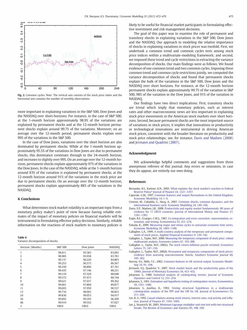
Fig. 2. Common cycles. Note: The vertical axis consists of the stock price index and thehorizontal axis contains the number of monthly observations.

475P.K. Narayan, K.S. Thuraisamy / Economic Modelling 35 (2013) 472–476

more important in explaining variations in the S&P 500, Dow Jones andthe NASDAQ over short-horizons. For instance, in the case of S&P 500,at the 1-month horizon approximately 98.9% of the variations areexplained by permanent shocks and at the 12-month horizon perma-nent shocks explain around 99.7% of the variations. Moreover, on anaverage over the 12-month period, permanent shocks explain over99% of the variations in the S&P 500.

In the case of Dow Jones, variations over the short horizon are alsodominated by permanent shocks. While at the 1-month horizon ap-proximately 95.5% of the variations in Dow Jones are due to permanentshocks, this dominance continues through to the 24-month horizon,and increases to slightly over 99%. On an average over the 12-month ho-rizon, permanent shocks explain approximately 97% of the variations intheDow Jones. In the case of theNASDAQ,while at the 1-month horizonaround 83% of the variation is explained by permanent shocks, at the12-month horizon around 91% of the variations in the stock price aredue to permanent shocks. On an average over the 12-month horizon,permanent shocks explain approximately 88% of the variations in theNASDAQ.

4. Conclusions

What determines stockmarket volatility is an important topic fromamonetary policy maker's point of view because having reliable esti-mates of the impact of monetary policies on financial markets will beinstrumental in formulating effective policy decisions. Similarly, reliableinformation on the reactions of stock markets to monetary policies is

Table 4Variance decomposition of shocks.

Horizon (Months) S&P 500 Dow Jones NASDAQ

1 98.811 95.583 83.0932 98.985 95.938 83.7813 99.137 96.220 84.8034 99.253 96.575 86.5675 99.350 96.896 87.7616 99.435 97.146 88.2217 99.510 97.320 88.6488 99.572 97.473 88.7449 99.621 97.637 89.26210 99.661 97.804 89.87711 99.693 97.950 90.53712 99.716 98.063 90.85324 99.836 99.053 94.91736 99.892 99.393 96.20948 99.919 99.552 97.027∞ 100.0 100.0 100.0

likely to be useful for financial market participants in formulating effec-tive investment and risk management decisions.

The goal of this paper was to examine the role of permanent andtransitory shocks in explaining variations in the S&P 500, Dow Jonesand the NASDAQ. Our approach to modeling the relative importanceof shocks in explaining variations in stock prices was twofold. First, weundertook a common trend and common cycles tests among stockprice indices within a multivariate-modeling framework; and second,we imposed these trend and cycle restrictions in extracting the variancedecomposition of shocks. Our main findings were as follows. We foundevidence of one common trend and two common cycles. Imposing thesecommon trend and common cycle restrictions jointly, we computed thevariance decomposition of shocks and found that permanent shocksexplain the bulk of the variations in the S&P 500, Dow Jones and theNASDAQ over short horizons. For instance, at the 12-month horizonpermanent shocks explain approximately 99.7% of the variation in S&P500, 98% of the variation in the Dow Jones, and 91% of the variation inNASDAQ.

Our findings have two direct implications. First, transitory shocksare trivial which imply that monetary policies, such as interestrates and other macroeconomic news are less important in explainingstock price movements in the American stock markets over short hori-zons. Second, because permanent shocks are themost important sourceof variations in stock prices, it implies that innovations in productivityor technological innovations are instrumental in driving Americanstock prices, consistent with the broader literature on productivity andstock price relationships; see, for instance, Davis and Madsen (2008)and Jermann and Quadrini (2007).

Acknowledgment

We acknowledge helpful comments and suggestions from threeanonymous referees of this journal. Any errors or omissions, in casethey do appear, are entirely our own doing.

References

Bernanke, B.S., Kuttner, K.N., 2005. What explains the stock market's reaction to FederalReserve Policy? Journal of Finance LX, 1221–1257.

Caporale, G.M., 1997. Common features and output fluctuations in the United Kingdom.Economic Modelling 14, 1–9.

Centoni, M., Cubadda, G., Hecq, A., 2007. Common shocks, common dynamics, and theinternational business cycle. Economic Modelling 24, 149–166.

Davis, E.P., Madsen, J.B., 2008. Productivity and equity market fundamentals: 80 years ofevidence for 11 OECD countries. Journal of International Money and Finance 27,1261–1283.

Engle, R.F., Granger, C.W.J., 1987. Co-integration and error correction: representation, es-timation, and testing. Econometrica 55, 251–276.

Fukuda, K., 2009. Measuring major and minor cycles in univariate economic time series.Economic Modelling 26, 1093–1100.

Gallagher, L.A., 1999. A multi-country analysis of the temporary and permanent compo-nents of stock prices. Applied Financial Economics 9, 129–142.

Gallagher, L., Taylor, M.P., 2000. Measuring the temporary component of stock price: robustmultivariate analysis. Economics Letters 67, 193–200.

Gallagher, L., Taylor, M.P., 2002a. The stock return-inflation puzzle revisited. EconomicsLetters 75, 147–156.

Gallagher, L., Taylor, M.P., 2002b. Permanent and temporary components of stock prices:evidence from assessing macroeconomic shocks. Southern Economic Journal 69,345–362.

Harvey, D.I., Mills, T.C., 2002. Common features in UK sectoral output. Economic Model-ling 19, 91–104.

Jermann, U.J., Quadrini, V., 2007. Stock market boom and the productivity gains of the1990s. Journal of Monetary Economics 54, 413–432.

Johansen, S., 1988. Statistical analysis of cointegrating vectors. Journal of EconomicDynamics and Control 12, 231–254.

Johansen, S., 1991. Estimation and hypothesis testing of cointegration vectors. Econometrica59, 1551–1580.

Johansen, S., Juselius, K., 1992. Testing structural hypotheses in a multivariatecointegration analysis of the PPP and the UIP for UK. Journal of Econometrics 53,211–244.

Lee, B.-S., 1992. Causal relations among stock returns, interest rates, real activity and infla-tion. Journal of Finance 47, 1591–1603.

Lee, J., Strazicich, M., 2003. Minimum Lagrangemultiplier unit root test with two structuralbreaks. The Review of Economics and Statistics 85, 108–109.

476 P.K. Narayan, K.S. Thuraisamy / Economic Modelling 35 (2013) 472–476

Lumsdaine, R.L., Papell, D.H., 1997. Multiple trend breaks and the unit-root hypothesis.The Review of Economics and Statistics 79, 212–218.

Manfredi, P., Fanti, L., 2004. Cycles in dynamic economic modelling. Economic Modelling21, 573–594.

Narayan, P.K., 2008. An investigation of the behaviour of Australia's business cycle.Economic Modelling 25, 676–683.

Narayan, P.K., 2010. What drives stock markets over short horizons? Evidence fromemerging markets. Quantitative Finance 11, 261–269.

Narayan, P.K., Popp, S., 2010. A new unit root test with two structural breaks in level andslope at unknown time. Journal of Applied Statistics 37, 1425–1438.

Narayan, P.K., Popp, S., 2013. Size and power properties of structural break unit root tests.Applied Economics 45, 721–728.

Perron, P., 1989. The great crash, the oil price shock and the unit root hypothesis.Econometrica 57, 1361–1401.

Rapach, D.E., 2001. Macro shocks and real stock prices. Journal of Economics and Business53, 5–26.

Rigobon, R., Sack, B., 2004. The impact of monetary policy on asset prices. Journal of Mon-etary Economics 51, 1553–1575.

Vahid, F., Engle, R.F., 1993. Common trends and common cycles. Journal of Applied Econo-metrics 8, 341–360.