Commun Nonlinear Sci Numer Simulat 19 (2014) 3938–3953

Contents lists available at ScienceDirect

Commun Nonlinear Sci Numer Simulat

journal homepage: www.elsevier .com/locate /cnsns

Fractional-order theory of heat transport in rigid bodies

http://dx.doi.org/10.1016/j.cnsns.2014.04.0041007-5704/� 2014 Elsevier B.V. All rights reserved.

⇑ Address: Dipartimento di Ingegneria Civile, Ambientale, Aerospaziale, dei Materiali, Viale delle Scienze Ed.8, 90128 Palermo, Italy. Tel.:23896763.

E-mail address: massimiliano.zingales@unipa.it

Massimiliano Zingales ⇑Dipartimento di Ingegneria Civile, Ambientale, Aerospaziale, dei Materiali, Viale delle Scienze Ed.8, 90128 Palermo, ItalyBio-Nanomechanics in Medicine (BNM2) Laboratory, Mediterranean Center of Human Health and Advanced Biotechnologies (MED-CHHAB),Viale delle Scienze Ed.18, 90128 Palermo, Italy

a r t i c l e i n f o a b s t r a c t

Article history:Received 7 October 2013Received in revised form 16 April 2014Accepted 17 April 2014Available online 30 April 2014

Keywords:Fractional derivativesNon-local thermodynamicsGeneralized entropyTemperature fieldNon-local temperature gradients

The non-local model of heat transfer, used to describe the deviations of the temperaturefield from the well-known prediction of Fourier/Cattaneo models experienced in complexmedia, is framed in the context of fractional-order calculus. It has been assumed (Borinoet al., 2011 [53], Mongioví and Zingales, 2013 [54]) that thermal energy transport is dueto two phenomena: (i) A short-range heat flux ruled by a local transport equation; (ii) Along-range thermal energy transfer proportional to a distance-decaying function, to the rel-ative temperature and to the product of the interacting masses. The distance-decayingfunction is assumed in the functional class of the power-law decay of the distance yieldinga novel temperature equation in terms of a-order Marchaud fractional-order derivativeð0 6 a 6 1Þ. Thermodynamical consistency of the model is provided in the context of Clau-sius–Plank inequality. The effects induced by the boundary conditions on the temperaturefield are investigated for diffusive as well as ballistic local heat flux. Deviations of the tem-perature field from the linear distributions in the neighborhood of the thermostated zonesof small-scale conductors are qualitatively predicted by the used fractional-order heattransport model, as shown by means of molecular dynamics simulations.

� 2014 Elsevier B.V. All rights reserved.

1. Introduction

The need for non-local thermodynamics in physical sciences and engineering may be traced back to the mid of the lastcentury in the attempt to capture the experimental effects unpredicted by Fourier diffusion theory. Indeed several experi-mental observations of temperature field at metal interfaces as well as of the changes in conductivity parameters in theneighborhood of thermostated regions (Kapitsa phonon-scattering) shows a localization of temperature gradients close tothe borders [1].

Similar phenomena have been observed with molecular dynamics (MD) simulations of heat transfer in nanowires show-ing that the presence of thermostated regions involves a phonon–phonon scattering that modifies the conductivity propertyof the materials [2,3].

Such studies have been further developed toward the use of advanced mathematical tools as the fractional-order calculus[4] to capture memory [5,6] as well as non-local effects [7–9]. Indeed fractional (real) order integro-differential operatorshave been introduced more and more often in several contexts of physics and engineering for their capability to interpolateamong the well-known integer-order operators of classical differential calculus [10]. In this regard some applications may be

+39 091

M. Zingales / Commun Nonlinear Sci Numer Simulat 19 (2014) 3938–3953 3939

found in the study of temporal and spatial evolution of complex systems close to critical points [11–14] or in stochastic set-ting [15–17]. Fractional-order differential calculus is widely used, also, to model the mechanical behavior of polymers, gels,foams and glassy materials [18–22] but also to model the rheology of soft matter and biological tissues [23–25]. States andfree energies for non-linear geometries [26–30] in terms of fractional-order derivatives may also be formulated.

The long-tails of fractional operators have been used to formulate non-local stress–strain constitutive equations that are aparticularized version of the integral model of non-local elasticity [31,32]. The same feature has been also used by the authorand its research team to derive a mechanically-based fractional-order non-local elasticity in statics [33–36] and wave prop-agation contexts [37,38] (see e.g. [39] for a complete review).

The presence of spatial non-local effects, observed in heat transport framework, has been introduced by means of integralmodels involving, beside the local gradient of the temperature field, an integral convolution among the temperature gradientand a real-order attenuation function [40–42]. The non-local formulation, originally proposed by Eringen and his co-workers,has been used, recently, to model thermoelastic coupling in microelectromechanical resonators (MEMRS) [43,44]. Some gen-eralization of this theory may be useful to the analysis of small-scale systems accounting for second-sound effects [45–47]modeled with a first-order time derivative of the heat flux [48–50] and introducing a generalized entropy [51,52].

Very recently a non-local model of thermal energy transport has been proposed with a physical picture of heat transfer in1D setting. It has been assumed that the non-local residual in the balance equation is due to a volume integral over the bodydomain of the elementary long-range heat transport among adjacent and non-adjacent locations of the body [53]. The long-range thermal energy contribution is modeled as two point function PðnlÞ x; y; tð Þ that depends on: (i) A decaying functiondecreasing with the distance of the interacting elements; (ii) The relative temperatures among locations and (iii) The productof the masses at locations x and y [54].

In this paper it is shown that, assuming the decaying function in the functional class of power-laws of the distance, thebalance principle involves fractional-order non-local residuals. The correspondent temperature equation is obtained in termsof Marchaud-type fractional derivatives in unbounded domains. A different scenario appears as the thermal energy exchangein bounded domains is considered since only the integral contributions to the Marchaud fractional derivatives defined onbounded regions appear. It follows that the divergent algebraic contributions at the borders are not included in the formu-lation allowing for the position of non-homogeneous Dirichlet boundary conditions straightforwardly. Moreover the Neu-mann boundary conditions associated to the fractional-order temperature equation involve, only, the gradient of thetemperature field as in well-known local heat transport theories.

The effects induced by the non-homogeneous boundary condition is further investigated, in this paper, either for diffusiveand ballistic/diffusive thermal energy exchange. The numerical results reported in the analyses describe the temperaturefield in 1D rigid conductors showing that the proposed model of fractional-order thermal energy exchange may capturethe non-uniform temperature distribution observed in Kapitsa experiments as well as in molecular dynamics simulations.

2. The fractional model of thermal energy exchange in rigid bodies: the second law of thermodynamics

In this section the fractional-order model of thermal energy exchange is derived for a diffusive heat transport. In the firstpart of the section the balance equation as well as the second law of thermodynamics will be shortly recalled. The secondpart of the section is dedicated to a numerical simulation of the temperature field in a 1D rigid conductor in presence of long-range thermal energy transport. The effects of the differentiation order on the temperature field in bounded conductors havebeen addressed with a numerical simulation code.

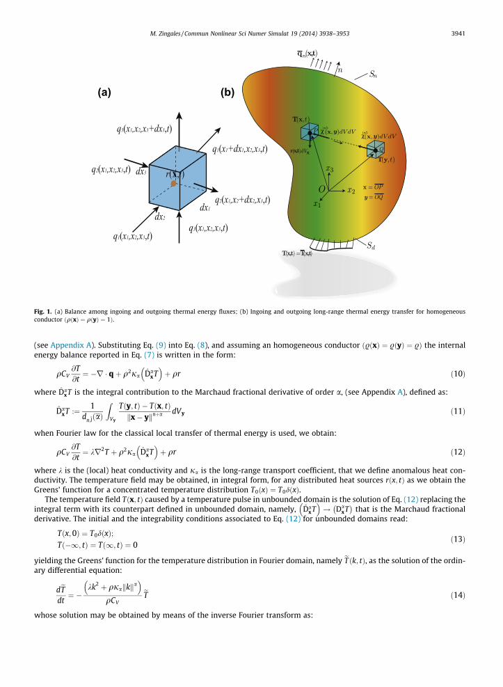
The main idea beyond the proposed model of non-local thermodynamics relies on the assumption that the energy balanceat location x 2 R3 of a rigid body, encapsulated in a subset V � R3 with boundary surface S ¼ @V , involves the followingcontributions:

1. The thermal energy flux among adjacent locations, that it is related to the divergence $ � qðx; tÞ of the heat flux densityvector qðx; tÞ.

2. A non-local energy transfer, due to the contribution of the elements y 2 R3 of the body, that it is assumed proportional tothe mass densities of the interacting elements at the locations x and y as

PðnlÞ x; y; tð Þ ¼ vðnlÞ x; y; tð ÞqðxÞqðyÞdVxdVy ð1Þ

where vðnlÞ x; y; tð ÞqðyÞdVy is the long-range specific energy per unit time transferred at locations x by the element at the loca-tion y and q is the mass density that is time-independent. Under some restriction of the functional dependence of the long-range specific energy PðnlÞ x; y; tð Þ, a Marchaud-type, fractional-order, non-local model of thermal energy transport is obtainedin unbounded domains. In bounded domains, instead, only integral parts of fractional-order operators are involved.

This latter consideration yields two key features of the fractional model of long-range heat transport: (i) The Non-Homoge-neous Dirichlet boundary conditions of the temperature field along the boundary Sd, namely Tðx; tÞ ¼ Tðx; tÞ with x 2 Sd maybe easily accounted for since the divergent algebraic contribution to the Marchaud fractional derivatives do not appear; (ii)The Neumann boundary conditions on the free surface Sn involves, only, the local contribution to the heat transfer in terms ofgradients of the temperature field r � Tðx; tÞ with x 2 Sn since the overall residual reads:

3940 M. Zingales / Commun Nonlinear Sci Numer Simulat 19 (2014) 3938–3953

ZVx

ZVy

vðnlÞ x; y; tð ÞqðyÞqðxÞdVydVx ¼ 0 ð2Þ

for any specific class of the specific long-range heat transport vðnlÞ x; y; tð ÞqðyÞdVy [54].

2.1. The fractional-order theory of Classical Irreversible Thermodynamics (CIT)

Let us consider an isotropic solid body with u :¼ u x; tð Þ the specific internal energy at location x and time t and let usassume that . ¼ .ðxÞ is the time-independent body density at location x as for closed thermodynamical system. The absolutetemperature of the body is denoted as Tðx; tÞ, and CV ¼ @u

@T

� �T0

is the volume specific heat at room temperature T0 assumedconstant in the analysis.

In the context of non-local thermodynamics we assume that, at location x ¼ x1; x2; x3ð Þ of the body, the internal energy ofthe body .ðxÞuðx; tÞ is composed by two contributes as:

@ .ðxÞuð Þ@t

¼ @ .ðxÞulð Þ@t

þ @ .ðxÞunlð Þ@t

ð3Þ

where we denoted .ðxÞulðx; tÞ and .ðxÞunlðx; tÞ the local and the long-range overall contribution to the internal energy atlocation x, respectively. In this regard the rate of change of the internal energy function in the balance equation (3) for aclosed thermodynamical system reads:

@u@t¼ @ul

@tþ @unl

@t¼ _wðx; tÞ þ _hðx; tÞ ¼ _hlðx; tÞ þ _hnlðx; tÞ ð4Þ

where _w ¼ 0 since rigid conductors are considered and _h is the rate of change of the specific thermal energy that is composedby a local _hlðx; tÞ and a long-range _hnlðx; tÞ term, respectively. The latter equality in Eq. (4) is the local version of first principleof thermodynamics in presence of long-range thermal energy transport yielding that the rate of change of the specific inter-nal energy _uðx; tÞ, equates the rate of change of the thermal energy _hðx; tÞ in any subdomain dVx of the conductor.

The proposed model of thermal energy transfer involves two main assumptions about the intrinsic state functions,namely, hlðx; tÞ and hnlðx; tÞ as:

� The rate of change of the local contribution qðxÞdVx_hlðx; tÞ depends on the thermal energy flux across the boundaries of

the control volume dVx, namely, qðx; tÞ as:

qðxÞ _hlðx; tÞ ¼ �r � qðx; tÞ þ qðxÞrðx; tÞ ð5Þ

with rðx; tÞ a specific thermal power source at location x as it may be easily withdrawn from the balance in Fig. 1(a).� The rate of change of the non-local thermal energy contribution qðxÞdVx

_hnlðx; tÞ is obtained as the resultant of the two-points exchange in Eq. (1), namely, PðnlÞ x; y; tð Þ (see Fig. 1(b)) yielding an additional thermal power source for the controlvolume dVx:

qðxÞdVx_hnlðx; tÞ ¼

ZVy

PðnlÞ x; y; tð Þ dVy ¼ qðxÞdVx

ZVy

vðnlÞ x; y; tð ÞqðyÞdVy ð6Þ

The first principle of thermodynamics introduced by Eqs. (1) and (6) may be obtained substituting Eqs. (5) and (6) into thebalance equation reported in Eq. (4) yielding:

qðxÞ @uðx; tÞ@t

¼ �r � qðx; tÞ þ qðxÞZ

Vy

vðnlÞ x; y; tð ÞqðyÞ dVy þ qðxÞrðx; tÞ ð7Þ

where the integral at the right-hand side is the non-local heat transfer contribute due to the interaction between the particlelocated at position x and all the other particles of the body [45].

The long-range contribution, namely function vðnÞl x; y; tð Þ, is the long-range thermal energy transfer and it depends on therelative temperature measured at locations x and y as:

vðnlÞ x; y; tð Þ ¼ jag kx� ykð Þ Tðy; tÞ � T x; tð Þ½ � ð8Þ

with ja a material dependent proportional coefficient and g kx� ykð Þ is a distance-decaying function accounting for thedecay of the long-range thermal energy transfer with the interdistance. In the following we assume that the functiong kx� ykð Þ decays as a power-law of the distance as:

g kx� ykð Þ ¼ 1dn;l að Þ

1kx� yknþa ð9Þ

where a 2 R; n 2 N is the dimension of the topological space of the body (in our case n ¼ 3) and the normalization coeffi-cient dn;l að Þ is related to the decaying exponent a and to the dimension of the topological space embedding the conductor n

(b)(a)

Fig. 1. (a) Balance among ingoing and outgoing thermal energy fluxes; (b) Ingoing and outgoing long-range thermal energy transfer for homogeneousconductor ðqðxÞ ¼ qðyÞ ¼ 1Þ.

M. Zingales / Commun Nonlinear Sci Numer Simulat 19 (2014) 3938–3953 3941

(see Appendix A). Substituting Eq. (9) into Eq. (8), and assuming an homogeneous conductor ð.ðxÞ ¼ .ðyÞ ¼ .Þ the internalenergy balance reported in Eq. (7) is written in the form:

qCV@T@t¼ �r � qþ q2ja D̂a

xT� �

þ qr ð10Þ

where D̂axT is the integral contribution to the Marchaud fractional derivative of order a, (see Appendix A), defined as:

D̂axT :¼ 1

dn;l að Þ

ZVy

Tðy; tÞ � T x; tð Þkx� yknþa dVy ð11Þ

when Fourier law for the classical local transfer of thermal energy is used, we obtain:

qCV@T@t¼ kr2T þ q2ja D̂a

xT� �

þ qr ð12Þ

where k is the (local) heat conductivity and ja is the long-range transport coefficient, that we define anomalous heat con-ductivity. The temperature field may be obtained, in integral form, for any distributed heat sources rðx; tÞ as we obtain theGreens’ function for a concentrated temperature distribution T0ðxÞ ¼ T0dðxÞ.

The temperature field Tðx; tÞ caused by a temperature pulse in unbounded domain is the solution of Eq. (12) replacing theintegral term with its counterpart defined in unbounded domain, namely, D̂a

xT� �

! DaxT

� �that is the Marchaud fractional

derivative. The initial and the integrability conditions associated to Eq. (12) for unbounded domains read:

Tðx;0Þ ¼ T0dðxÞ;Tð�1; tÞ ¼ Tð1; tÞ ¼ 0

ð13Þ

yielding the Greens’ function for the temperature distribution in Fourier domain, namely eT ðk; tÞ, as the solution of the ordin-ary differential equation:

deTdt¼ �

kk2 þ qjakkka� �

qCV

eT ð14Þ

whose solution may be obtained by means of the inverse Fourier transform as:

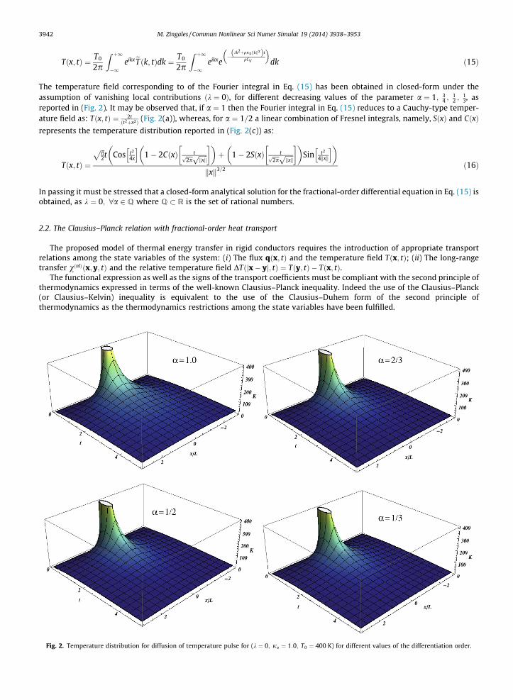
Fig.

3942 M. Zingales / Commun Nonlinear Sci Numer Simulat 19 (2014) 3938–3953

Tðx; tÞ ¼ T0

2p

Z þ1

�1eikxeT ðk; tÞdk ¼ T0

2p

Z þ1

�1eikxe

�kk2þqjakkkað Þt

qCV

� �dk ð15Þ

The temperature field corresponding to of the Fourier integral in Eq. (15) has been obtained in closed-form under theassumption of vanishing local contributions ðk ¼ 0Þ, for different decreasing values of the parameter a ¼ 1; 3

4 ;12 ;

13, as

reported in (Fig. 2). It may be observed that, if a ¼ 1 then the Fourier integral in Eq. (15) reduces to a Cauchy-type temper-ature field as: Tðx; tÞ ¼ 2t

ðt2þx2Þ (Fig. 2(a)), whereas, for a ¼ 1=2 a linear combination of Fresnel integrals, namely, SðxÞ and CðxÞrepresents the temperature distribution reported in (Fig. 2(c)) as:

Tðx; tÞ ¼

ffiffiffip2

pt Cos t2

4x

h i1� 2CðxÞ tffiffiffiffi

2pp ffiffiffiffiffi

kxkp

� � þ 1� 2SðxÞ tffiffiffiffi

2pp ffiffiffiffiffi

kxkp

� � Sin t2

4kxk

h i kxk3=2 ð16Þ

In passing it must be stressed that a closed-form analytical solution for the fractional-order differential equation in Eq. (15) isobtained, as k ¼ 0; 8a 2 Q where Q � R is the set of rational numbers.

2.2. The Clausius–Planck relation with fractional-order heat transport

The proposed model of thermal energy transfer in rigid conductors requires the introduction of appropriate transportrelations among the state variables of the system: (i) The flux qðx; tÞ and the temperature field Tðx; tÞ; (ii) The long-rangetransfer vðnlÞðx; y; tÞ and the relative temperature field DTðjx� yj; tÞ ¼ Tðy; tÞ � Tðx; tÞ.

The functional expression as well as the signs of the transport coefficients must be compliant with the second principle ofthermodynamics expressed in terms of the well-known Clausius–Planck inequality. Indeed the use of the Clausius–Planck(or Clausius–Kelvin) inequality is equivalent to the use of the Clausius–Duhem form of the second principle ofthermodynamics as the thermodynamics restrictions among the state variables have been fulfilled.

2. Temperature distribution for diffusion of temperature pulse for (k ¼ 0; ja ¼ 1:0; T0 ¼ 400 K) for different values of the differentiation order.

M. Zingales / Commun Nonlinear Sci Numer Simulat 19 (2014) 3938–3953 3943

The compatibility of the proposed model is assessed in terms of the entropy state function, namely, sðx; tÞ that must obeyto Clausius–Planck inequality for a thermodynamical system evolving from state A! B at time instants tA and tB, respec-tively, as:

MsABðxÞ ¼ sðx; tBÞ � s x; tAð Þ ¼Z tB

tA

q_sðx; tÞdt PZ tB

tA

dhðx; tÞTðx; tÞ ð17Þ

where we introduced the specific entropy function rate _sðx; tÞ and dh is the thermal energy increment of the body subdomainat location x. Recalling that, in a rigid body, s ¼ sðuÞ and that @s=@u ¼ 1=T , making use of the energy balance equation, theright hand side of Eq. (17) may be written in the form:

q_sðx; tÞP �$ � qðx; tÞTðx; tÞ þ

qðxÞrðx; tÞTðx; tÞ þ qðxÞ

Tðx; tÞ

ZVy

qðyÞvðnlÞ x; y; tð ÞdVy ð18Þ

The observation of Eq. (18) for the specific entropy rate increment shows that an additional contribution at the right-handside is obtained with respect to the classical expression of the Clausius–Planck inequality. Eq. (18) may be recast in a moreconvenient form, introducing the specific entropy rate production rðsÞðx; tÞP 0 for any thermodynamical process yielding:

q_sðx; tÞ þ $ � qðx; tÞTðx; tÞ �

qðxÞrðx; tÞTðx; tÞ � qðxÞ

Tðx; tÞ

ZVy

qðyÞvðnlÞ x; y; tð ÞdVy ¼ qrðsÞðx; tÞP 0 ð19Þ

On the other hand the entropy rate may be expressed at location x in the form of a balance among the incoming and theoutcoming entropy flux in the unitary time so that:

q_sðx; tÞ ¼ �$ � JðsÞl ðx; tÞ þZ

Vy

JðsÞnl x; y; tð ÞdVy þqðxÞrðx; tÞ

Tðx; tÞ þ qðxÞrðsÞðx; tÞ ð20Þ

where we introduced the local and non-local long-range entropy transfer, respectively, JðsÞl ðx; tÞ and JðsÞnl x; y; tð Þ related to thelocal and long-range thermal energy transfer, respectively.

Eq. (20) may be substituted into Eq. (18) to yield the inequality:

�$ � qðx; tÞTðx; tÞ þ

qðxÞTðx; tÞ

ZVy

qðyÞvðnlÞ x; y; tð ÞdVy þ $ � JðsÞl ðx; tÞ �Z

Vy

JðsÞnl x; y; tð ÞdVy P 0 ð21Þ

The entropy flux is assumed to be a function of state of the local contribution to the internal energy rateJðsÞl ðxÞ ¼ ul ulð ÞqlðxÞ and, by similar considerations we will assume that the long-range entropy transfer is provided asJðsÞnl x; yð Þ ¼ unl unlð Þ.2vðnlÞ x; yð Þ (assuming qðxÞ ¼ q). Under these circumstances the expression in Eq. (21), omitting thedependence on the time variabile t, yields:

ul ulð Þ �1

TðxÞ

$ � qðxÞ þ qðxÞ � r ul ulð Þð Þ �

ZVy

unl unlð Þ � .2vðnlÞ x; yð ÞTðxÞ

dVy P 0 ð22Þ

The inequality restriction in Eq. (22) leads to the conclusion that the linear term involving the thermal energy flux qðx; tÞmust vanish yielding the relation:

ul ulð Þ ¼1

Tðx; tÞ ð23Þ

that, upon substitution into Eq. (22) it yields:

qðx; tÞT2ðx; tÞ

� r Tðx; tÞð Þ þZ

Vy

unl unlð Þ � 1Tðx; tÞ

.2vðnlÞ x; y; tð ÞdVy 6 0 ð24Þ

The inequality in Eq. (24) for the entropy production may be fulfilled if, for the first term, we assume a linear force-flux rela-tion as:

q x; tð Þ ¼ �k$ Tðx; tÞð Þ ð25Þ

with k P 0 that corresponds to Fourier relation, whereas, the second term at right hand side must involve the inverse of atemperature field 1=T for dimensionality sake. As we assume that the long-range entropy flux function unl unlð Þ ¼ 1=T y; tð Þsince JðsÞnl x; y; tð Þ represents the entropy variation at location x due to a thermal source at location y, then the integral termmust satisfy the inequality:

Z

Vy

Tðx; tÞ � T y; tð ÞTðx; tÞT y; tð Þ

vðnlÞ x; y; tð ÞdVy 6 0 ð26Þ

that is fulfilled if a linear force-flux relation for the long-range thermal energy transfer is assumed in Eq. (8):vðnlÞ x; y; tð Þ ¼ g kx� ykð Þ T y; tð Þ � T x; tð Þ½ � and g kx� yk; tð ÞP 0 as in Eq. (9). Such restrictions for the local and non-local ther-

3944 M. Zingales / Commun Nonlinear Sci Numer Simulat 19 (2014) 3938–3953

mal energy exchanges are satisfied with the power-law decaying function g x; yð Þ defined in Eq. (9) that is compliant with thesecond principle of thermodynamics [47].

2.3. Numerical simulation: temperature distribution in 1D rigid conductor

The field of temperature distribution Tðx; tÞ ruled by Eq. (13) in a bounded 1D domain of length L is provided by the solu-tion of the fractional differential equation that reads (omitting arguments):

qCV@T@t¼ kr2T þ qja D̂a

x T� �

ð27Þ

where only the integral parts of the Marchaud fractional derivatives are involved. In this case the analysis of the temperaturefield is obtained resorting to the fractional finite difference (FFD) discretization of fractional derivative operator. Indeed, aswe introduce a discrete grid of abscissas xj ¼ ðj� 1ÞDx, with step Mx ¼ L= N þ 1ð Þ the finite difference solution of the non-localtemperature field will be obtained at the gridpoints xj; ðj ¼ 1;2; . . . ;N þ 1Þ introducing the central finite difference operatorsfor the second-order gradient and the FFD approximation of the D-Riesz fractional derivative as:

@2f xj� �

@x2 wD2fj

Dx2 ¼f xjþ1� �

� 2f xj� �þ f xj�1� �

Dx2 ð28Þ

D̂ax f

� �xj� �wDa

x f xj� �¼ a�1

C 1� að ÞXj�1

h¼1xj�hþ1� ��a � xj�h

� ��ah i

f xhð Þn o

þ a�1

C 1� að ÞXNþ1

h¼jþ1xh�j� ��a � xh�j�1

� ��ah i

f xhð Þn o

ð29Þ

Introduction of the finite difference scheme in the governing equation of the temperature field in Eq. (28) yields a set ofordinary differential equations in time domain in the form:

_T tð Þ þ KðlÞ þ KðnlÞh i

TðtÞ ¼ �r tð Þ ð30Þ

where T tð Þ ¼ T1 tð Þ T2 tð Þ . . . . . . TNþ1 tð Þ½ �T is a vector collecting the values of the temperature field at the grid pointswith initial conditions in the form Tð0Þ ¼ T0 and �r tð Þ is a vector gathering the values of the heat source in the conductordomain with elements �rjðtÞ ¼ rðxj; tÞ=CV . The N þ 1ð Þ � N þ 1ð Þ local and non-local diffusion matrices reported in Eq. (30)read, respectively:

KðlÞ ¼ k

CV ðDxÞ2

1 �1 0 . . . . . . 0�1 2 �1 . . . . . . 0. . . . . . . . . . . . . . . . . .

. . . . . . . . . . . . . . . . . .

0 . . . 0 �1 2 �10 0 . . . . . . �1 1

2666666664

3777777775ð31Þ

KðnlÞ ¼ jaaCVC 1� að Þ

KðnlÞ11 KðnlÞ

12 KðnlÞ13 . . . . . . KðnlÞ

1Nþ1

Sym KðnlÞ22 KðnlÞ

23 . . . . . . KðnlÞ2Nþ1

. . . . . . . . . . . . . . . . . .

. . . . . . . . . . . . . . . . . .

Sym . . . KðnlÞNN . . .

Sym . . . . . . . . . Sym KðnlÞNþ1Nþ1

266666666664

377777777775ð32Þ

where KðnlÞjh ¼ xj�hþ1

� ��a � xj�h� ��a and with the diagonal terms in Eq. (32) that read KðnlÞ

jj ¼ �PNþ1

h–jh¼1

KðnlÞjh . The differential

equation reported in Eq. (30) has been solved with the approximate integration scheme provided by FFD for constant tem-peratures at the boundaries as:

Tð�L=2; tÞ ¼ T2 ¼ 200 K TðL=2; tÞ ¼ T1 ¼ 100 K ð33Þ

with initial conditions provided as a linear distributions of temperatures among the values T2 and T1 as:

Tðx;0Þ ¼ T2 �ð1þ 2x=LÞ T2 � T1ð Þ

2ð34Þ

The corresponding numerical solution of the boundary value problem reported in Eq. (27) and in Eqs. (33) and (34) has beenreported in (Fig. 3) for different values of the differentiation index a. It may be observed that, introducing long-range thermal

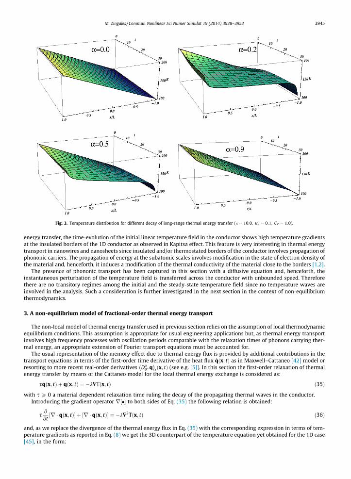
Fig. 3. Temperature distribution for different decay of long-range thermal energy transfer (k ¼ 10:0; ja ¼ 0:1; CV ¼ 1:0).

M. Zingales / Commun Nonlinear Sci Numer Simulat 19 (2014) 3938–3953 3945

energy transfer, the time-evolution of the initial linear temperature field in the conductor shows high temperature gradientsat the insulated borders of the 1D conductor as observed in Kapitsa effect. This feature is very interesting in thermal energytransport in nanowires and nanosheets since insulated and/or thermostated borders of the conductor involves propagation ofphononic carriers. The propagation of energy at the subatomic scales involves modification in the state of electron density ofthe material and, henceforth, it induces a modification of the thermal conductivity of the material close to the borders [1,2].

The presence of phononic transport has been captured in this section with a diffusive equation and, henceforth, theinstantaneous perturbation of the temperature field is transferred across the conductor with unbounded speed. Thereforethere are no transitory regimes among the initial and the steady-state temperature field since no temperature waves areinvolved in the analysis. Such a consideration is further investigated in the next section in the context of non-equilibriumthermodynamics.

3. A non-equilibrium model of fractional-order thermal energy transport

The non-local model of thermal energy transfer used in previous section relies on the assumption of local thermodynamicequilibrium conditions. This assumption is appropriate for usual engineering applications but, as thermal energy transportinvolves high frequency processes with oscillation periods comparable with the relaxation times of phonons carrying ther-mal energy, an appropriate extension of Fourier transport equations must be accounted for.

The usual representation of the memory effect due to thermal energy flux is provided by additional contributions in thetransport equations in terms of the first-order time derivative of the heat flux _q x; tð Þ as in Maxwell–Cattaneo [42] model orresorting to more recent real-order derivatives Da

0þq� �

t x; tð Þ (see e.g. [5]). In this section the first-order relaxation of thermalenergy transfer by means of the Cattaneo model for the local thermal energy exchange is considered as:

s _q x; tð Þ þ q x; tð Þ ¼ �k$T x; tð Þ ð35Þ

with s P 0 a material dependent relaxation time ruling the decay of the propagating thermal waves in the conductor.Introducing the gradient operator r �½ � to both sides of Eq. (35) the following relation is obtained:

s @@tr � q x; tð Þ½ � þ r � q x; tð Þ½ � ¼ �k$2T x; tð Þ ð36Þ

and, as we replace the divergence of the thermal energy flux in Eq. (35) with the corresponding expression in terms of tem-perature gradients as reported in Eq. (8) we get the 3D counterpart of the temperature equation yet obtained for the 1D case[45], in the form:

3946 M. Zingales / Commun Nonlinear Sci Numer Simulat 19 (2014) 3938–3953

sqCV@2T x; tð Þ@t2 þ @

@tqCV T x; tð Þ � ska D̂aT x; tð Þ

� �� �¼ k$2T x; tð Þ þ ka D̂aT x; tð Þ

� �þ qr x; tð Þ þ _qr x; tð Þ ð37Þ

The use of Eq. (35) for local thermal energy transfer q x; tð Þ involves non-monotonic increments of the entropy functions ¼ sðuÞ of CIT introduced in previous section as observed in previous papers [39,40]. Previous consideration leads to assessthe thermodynamical consistency of the model in terms of the extended irreversible thermodynamics (EIT) as it is shown inthe following section.

3.1. The Clausius–Planck relation of EIT with fractional-order heat transport

The introduction of a first-order time lag in the force-flux relation (Eq. (35)), requires the introduction of a non-equilib-rium entropy, functionally dependent on the internal energy density u and on the thermal energy flux q in the form:s ¼ s u;qð Þ. Under this assumption the local entropy flux shows the functional dependence JðsÞl ¼ JðsÞl u;qð Þ ¼ uðuÞq [28]. In thissetting, the non-equilibrium entropy rate reads:

_s ¼ _s u;qð Þ ¼ @s@u

q

_uþ @s@q

u

_q ð38Þ

In the following we assume an isotropic body so that the functional dependence entropy function and local entropy flux maybe assumed as: s ¼ s u;q � qð Þ ¼ s u; q2

� �and: JðsÞl ¼ JðsÞl u; q2

� �, respectively. Under these circumstances the entropy rate func-

tion in Eq. (38) may be written as:

_s ¼ _s u; q2� �¼ @s

@u

q2

_uþ @s@q2

u2q � _q ð39Þ

Substitution of Eq. (39) into the entropy balance equation reported in Eq. (27) yields (omitting the dependence on the timevariable):

qðxÞ @s@u

q2

_uþ q@s@q2

u

2q � _qþ $ � JðsÞl ðxÞ �Z

Vy

JðsÞnl x; yð ÞdVy �qr

TðxÞ ¼ qðxÞrðsÞðx; tÞ ð40Þ

As we substitute, for the rate of internal energy, the expression in terms of the local and long-range thermal energy fluxes inEq. (8) and accounting for Cattaneo transport equation in Eq. (35), after straightforward manipulations we get:

@s@u

q2

�r � qþ qðxÞZ

Vy

qðyÞvðnlÞ x; yð ÞdVy þ qr

!þ q

@s@q2

u2q � _qþ $ � JðsÞl ðxÞ �

ZVy

JðsÞnl x; yð ÞdVy �qðxÞrTðxÞ

¼ qðxÞrðsÞðx; tÞ ð41Þ

The derivative of the entropy function with respect to the internal energy, @s@u

� �q2 , is, dimensionally, a temperature field and

under the assumption in Eq. (38) it may be selected as the absolute temperature of the body: @s@u

� �q2 ¼ 1

TðxÞ yielding Eq. (41) inthe form:

�r � qTðxÞ þ

qðxÞTðxÞ

ZVy

qðyÞvðnlÞ x; yð ÞdVy � qðxÞ @s@q2

u2q � k

srT þ q

s

þ $ � JðsÞl ðxÞ �

ZVy

JðsÞnl x; yð ÞdVy ¼ qðxÞrðsÞðx; tÞ ð42Þ

Right-hand side of Eq. (42), namely entropy production rate, must be positive, so that, after some manipulation, the follow-ing inequality reads:

ul �1

TðxÞ

r � q�

ZVy

JðsÞnl x; yð Þ � qðxÞqðyÞvðnlÞ x; yð ÞTðxÞ

dVy �

2qðxÞks

@s@q2

2q � ðrTÞ

� 2qðxÞs

@s@q2

q2 þ $ulð Þ � q P 0 ð43Þ

where JðsÞl ¼ ulðuÞq. The condition in Eq. (43) may be respected as function ulðuÞ ¼ 1TðxÞ yielding the following inequality for

the remaining terms:

ZVy

JðsÞnl x; yð Þ � q2vðnlÞ x; yð ÞTðxÞ

dVy þ

2qks

q � ðrTÞ þ 2qs

q2

@s@q2

þ $TðxÞ

TðxÞ2� q 6 0 ð44Þ

that must be fulfilled for any thermodynamical process in the body.The first term in Eq. (44) is analogous to Eq. (24) and assuming JðsÞnl x; yð Þ ¼ unlðuÞqðxÞqðyÞvðnlÞ x; yð Þ the condition on the

proportionality function unlðuÞ yields: unlðuÞ ¼ 1TðyÞ to respect the Clausius–Planck inequality in Eq. (44) for any thermody-

namical process. As a consequence the decaying function g x; nð ÞP 0 as in previous section. The second term in Eq. (44) sat-isfies the inequality sign as:

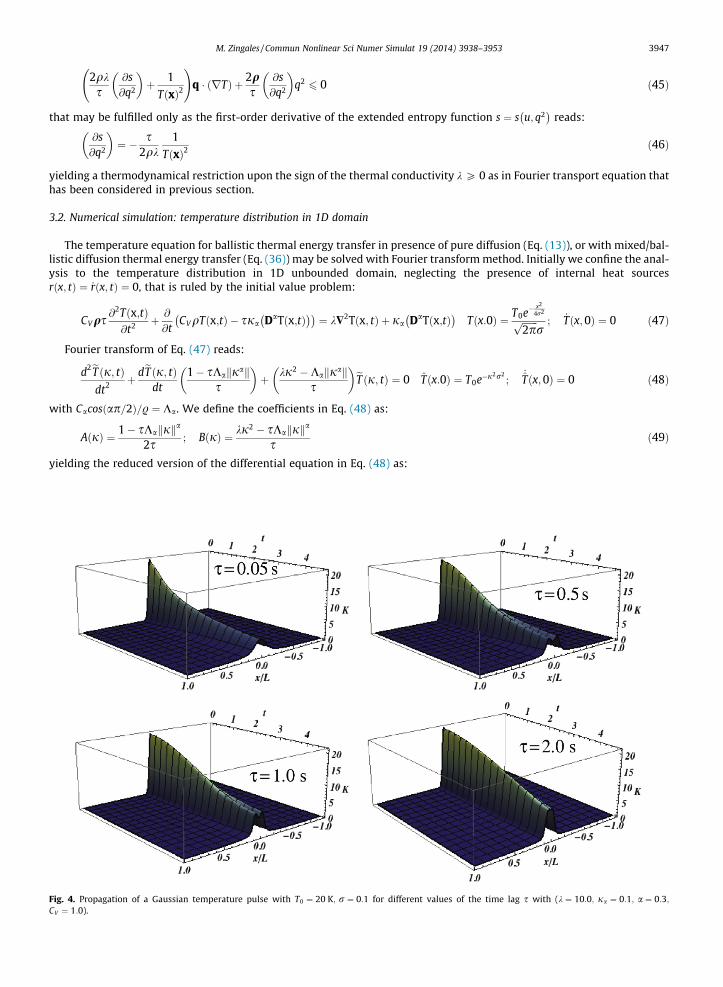
Fig. 4.CV ¼ 1:

M. Zingales / Commun Nonlinear Sci Numer Simulat 19 (2014) 3938–3953 3947

2qks

@s@q2

þ 1

TðxÞ2

!q � ðrTÞ þ 2q

s@s@q2

q26 0 ð45Þ

that may be fulfilled only as the first-order derivative of the extended entropy function s ¼ s u; q2� �

reads:

@s@q2

¼ � s

2qk1

TðxÞ2ð46Þ

yielding a thermodynamical restriction upon the sign of the thermal conductivity k P 0 as in Fourier transport equation thathas been considered in previous section.

3.2. Numerical simulation: temperature distribution in 1D domain

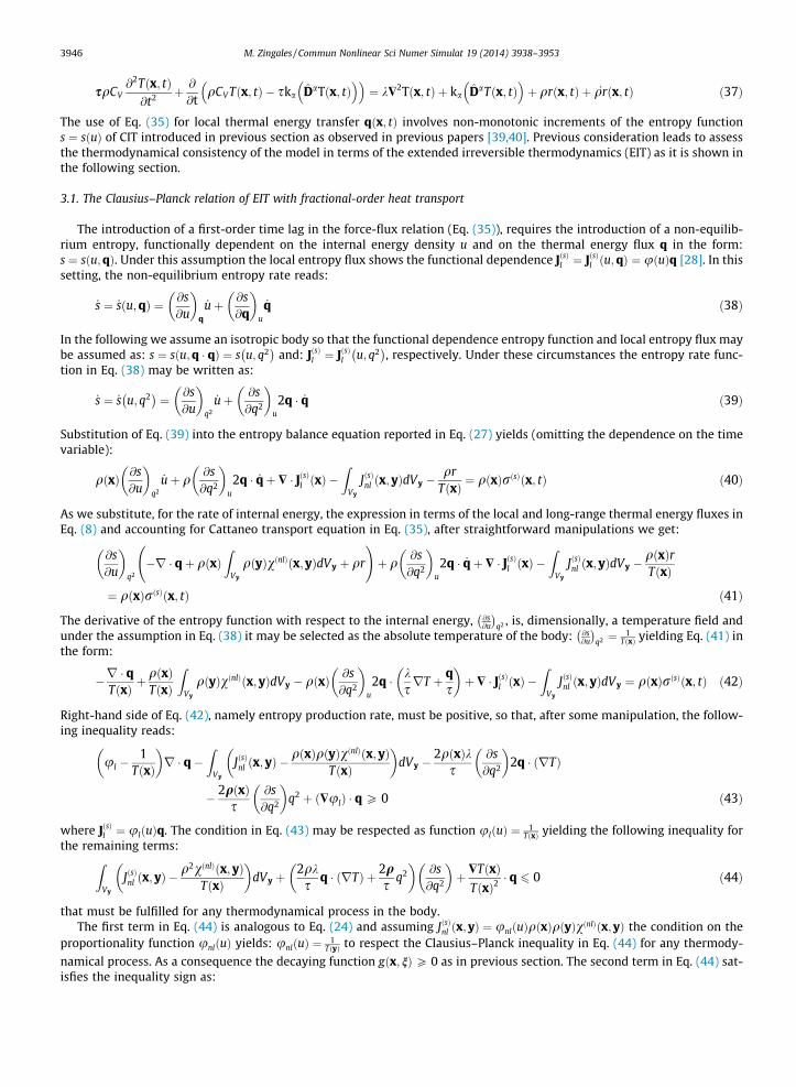
The temperature equation for ballistic thermal energy transfer in presence of pure diffusion (Eq. (13)), or with mixed/bal-listic diffusion thermal energy transfer (Eq. (36)) may be solved with Fourier transform method. Initially we confine the anal-ysis to the temperature distribution in 1D unbounded domain, neglecting the presence of internal heat sourcesrðx; tÞ ¼ _rðx; tÞ ¼ 0, that is ruled by the initial value problem:

CVqs @2T x;tð Þ@t2 þ @

@tCVqT x;tð Þ � sja DaT x;tð Þ

� �� �¼ k$2T x; tð Þ þ ja DaT x;tð Þ

� �T x:0ð Þ ¼ T0e�

x2

4r2ffiffiffiffiffiffiffi2pp

r; _Tðx;0Þ ¼ 0 ð47Þ

Fourier transform of Eq. (47) reads:

d2eT j; tð Þdt2 þ deT j; tð Þ

dt1� sKakjak

s

þ kj2 �Kakjak

s

eT j; tð Þ ¼ 0 T̂ x:0ð Þ ¼ T0e�j2r2;

_̂Tðx;0Þ ¼ 0 ð48Þ

with Cacos ap=2ð Þ=. ¼ Ka. We define the coefficients in Eq. (48) as:

A jð Þ ¼ 1� sKakjka

2s ; B jð Þ ¼ kj2 � sKakjka

s ð49Þ

yielding the reduced version of the differential equation in Eq. (48) as:

Propagation of a Gaussian temperature pulse with T0 ¼ 20 K; r ¼ 0:1 for different values of the time lag s with (k ¼ 10:0; ja ¼ 0:1; a ¼ 0:3;0).

Fig. 5.

3948 M. Zingales / Commun Nonlinear Sci Numer Simulat 19 (2014) 3938–3953

d2eT j; tð Þdt2 þ A jð Þd

eT j; tð Þdt

þ B jð ÞeT j; tð Þ ¼ 0 T̂ðx;0Þ ¼ T0e�j2r2;

_̂Tðx;0Þ ¼ 0 ð50Þ

whose solution is provided as usual linear combination of exponential functions with coefficients dependent on the initialconditions. In this regard the temperature distribution is provided, in Fourier domain as:

T x;tð Þ ¼ T0

2p

Z þ1

�1

r2 jð Þer1 jð Þt � r1 jð Þer2 jð Þt

r1 jð Þ � r2 jð Þ e�j2r2eijxdj ð51Þ

where r1 jð Þ and r2 jð Þ are the solution of the characteristic equation expressed in terms of the coefficients A jð Þ and B jð Þ as:

r1 jð Þ ¼ � A jð Þ þffiffiffiffiffiffiffiffiffiffiffiffiffiffiffiffiffiffiffiffiffiffiffiffiffiffiffiffiA jð Þ2 � B jð Þ

q ; r2 jð Þ ¼ � A jð Þ �

ffiffiffiffiffiffiffiffiffiffiffiffiffiffiffiffiffiffiffiffiffiffiffiffiffiffiffiffiA jð Þ2 � B jð Þ

q ð52Þ

The presence of time lag s in thermal energy transport induces the propagation of a decaying thermal wave that is stronglyinfluenced by the fractional-order transport represented by integral terms in Eq. (50). The effects of the fractional differen-tiation order in the temperature distribution is reported in (Fig. 4(a)–(d)) showing the presence of a thermal wave propagat-ing in 1D domain with a faster decay induced by the long-range diffusive transport. The effects induced by the time lag s inthe temperature distribution of local and non-local type is showed in (Figs. 5(a)–(d)) reporting the temperatures of a 1Ddomain for different values of the time lag s ¼ 0; s ¼ 0:05 s; s ¼ 0:5 s; s ¼ 5 sð Þ. It is shown that, as time lag increases, someof the thermal energy is transferred by diffusion (smaller values of s) among adjacent and non-adjacent locations whereassome other is transferred by ballistic motion of thermal phonons. In case of larger values of the time lags, the presence ofdamped thermal waves corresponding to ballistic motion increases over classical diffusion (5(c)–(d)).

The study of the temperature field in an 1D bounded domain is ruled by the second-order integro-differential equationcontaining the integral parts of the Marchaud derivatives as:

CVqs @2T x;tð Þ@t2 þ @

@tCVqT x;tð Þ � sja D̂aT x;tð Þ

� �� �¼ k$2T x; tð Þ þ ja D̂aT x;tð Þ

� �ð53Þ

The numerical analyses reported in the paper aim to highlight the effects of the time-lag s and of the coefficient a on thetemperature field as well as on the propagation of thermal waves induced by initial disturbances. The temperature fieldhas been obtained resorting to the FFD scheme introducing the discretization grid with N þ 1 node and step Dx ¼ L

ðNþ1Þ thetemperature values at the nodes, namely, Tj tð Þ with j ¼ 1;2; . . . N þ 1 are provided as solution of the differential equations:

s€T tð Þ þ CðlÞ þ CðnlÞh i

_T tð Þ þ KðlÞ þ KðnlÞh i

TðtÞ ¼ �r tð Þ ð54Þ

Temperature distribution with long-range thermal energy transfer for different values of the differentiation order a (k ¼ 10:0; ja ¼ 0:1; CV ¼ 1:0).

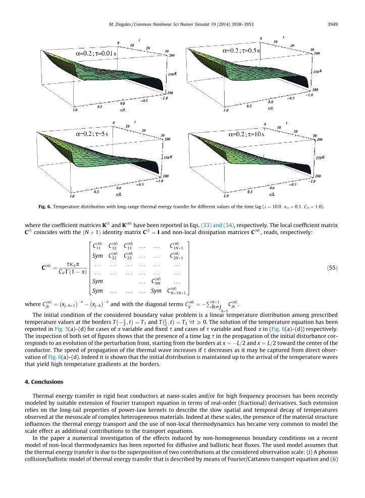
Fig. 6. Temperature distribution with long-range thermal energy transfer for different values of the time lag (k ¼ 10:0; ja ¼ 0:1; CV ¼ 1:0).

M. Zingales / Commun Nonlinear Sci Numer Simulat 19 (2014) 3938–3953 3949

where the coefficient matrices KðlÞ and KðnlÞ have been reported in Eqs. (33) and (34), respectively. The local coefficient matrixC lð Þ coincides with the ðN þ 1Þ identity matrix CðlÞ ¼ I and non-local dissipation matrices CðnlÞ, reads, respectively:

CðnlÞ ¼ sjaaCVC 1� að Þ

CðnlÞ11 CðnlÞ

12 CðnlÞ13 . . . . . . CðnlÞ

1Nþ1

Sym CðnlÞ22 CðnlÞ

23 . . . . . . CðnlÞ2Nþ1

. . . . . . . . . . . . . . . . . .

. . . . . . . . . . . . . . . . . .

Sym . . . CðnlÞNN . . .

Sym . . . . . . . . . Sym CðnlÞNþ1Nþ1

266666666664

377777777775ð55Þ

where CðnlÞjh ¼ xj�hþ1

� ��a � xj�h� ��a and with the diagonal terms CðnlÞ

jj ¼ �PNþ1

h–jh¼1

CðnlÞjh .

The initial condition of the considered boundary value problem is a linear temperature distribution among prescribedtemperature values at the borders T � L

2 ; t� �

¼ T1 and T L2 ; t� �

¼ T2 8t P 0. The solution of the temperature equation has beenreported in Fig. 5(a)–(d) for cases of a variable and fixed s and cases of s variable and fixed a in (Fig. 6(a)–(d)) respectively.The inspection of both set of figures shows that the presence of a time lag s in the propagation of the initial disturbance cor-responds to an evolution of the perturbation front, starting from the borders at x ¼ �L=2 and x ¼ L=2 toward the center of theconductor. The speed of propagation of the thermal wave increases if s decreases as it may be captured from direct obser-vation of Fig. 6(a)–(d). Indeed it is shown that the initial distribution is maintained up to the arrival of the temperature wavesthat yield high temperature gradients at the borders.

4. Conclusions

Thermal energy transfer in rigid heat conductors at nano-scales and/or for high frequency processes has been recentlymodeled by suitable extension of Fourier transport equation in terms of real-order (fractional) derivatives. Such extensionrelies on the long-tail properties of power-law kernels to describe the slow spatial and temporal decay of temperaturesobserved at the mesoscale of complex heterogeneous materials. Indeed at these scales, the presence of the material structureinfluences the thermal energy transport and the use of non-local thermodynamics has became very common to model thescale effect as additional contributions to the transport equations.

In the paper a numerical investigation of the effects induced by non-homogeneous boundary conditions on a recentmodel of non-local thermodynamics has been reported for diffusive and ballistic heat fluxes. The used model assumes thatthe thermal energy transfer is due to the superposition of two contributions at the considered observation scale: (i) A phononcollision/ballistic model of thermal energy transfer that is described by means of Fourier/Cattaneo transport equation and (ii)

3950 M. Zingales / Commun Nonlinear Sci Numer Simulat 19 (2014) 3938–3953

a phononic small-scale heat transport accounting for the long-range thermal energy transfer proportional to the relativetemperature among interacting locations, to the product of interacting masses and to a proper, material-type decaying func-tion. Restrictions on the functional class of the distance-decaying function have been reported in the paper showing that anydecaying function that is strictly positive in the whole conductors’ domain is eligible in terms of the Clausius–Planckinequality.

As we assume that the decaying function belongs to the functional class of power-laws of the interacting distances then afractional-order heat equation with Marchaud-type fractional derivatives of order a� 0;1½ � is obtained in unboundeddomains. A different scenario appears as bounded conductors are considered since only integral terms of Marchaud frac-tional operator are retained in the model. This aspect is a peculiarity of the proposed long-range thermal energy transfer thatprevent for the ill-conditioning of non-homogeneous Dirichlet and Neumann boundary conditions always encountered inintegral non-local approaches.

It is shown that the proposed model yields the phonon–phonon scattering of thermal energy waves outside the thermo-statted regions where the changes of the electron density modifies the material conduction parameters yielding a non-uni-form temperature field. The model may be extended to coupled thermoelastic problems to highlight the effects of the non-homogeneous temperature distribution on the stress and strain field observed in materials at the nanoscale.

Acknowledgments

The author is very grateful to the financial support provided by the PRIN2010-11 ‘‘Stability, Control and Reliability ofFlexible Structures’’ with National Coordinator Prof. A. Luongo. Stimulating discussions with Prof. Mario Di Paola are alsogratefully acknowledged.

Appendix A. Remarks on fractional calculus

In this appendix the essential features of fractional calculus will be shortly discussed.Let us consider a real-valued, Lebesgue integrable function f ðxÞ; x 2 R such that f ðxÞ 2 L1. The left and right Riemann–

Liouville (RL) fractional-order integrals are defined as:

Iaþf� �

ðxÞ ¼ 1C að Þ

Z x

�1

f yð Þx� yð Þ1�a dy

Ia�f� �

ðxÞ ¼ 1C að Þ

Z 1

x

f yð Þy� xð Þ1�a dy

ð56Þ

with a 2 0;1½ � and C �ð Þ is the Euler-Gamma function. The left and right fractional derivatives are defined as:

Daþf

� �ðxÞ ¼ 1

C 1� að Þddx

Z x

�1

f yð Þx� yð Þ1�a dy

Da�f

� �ðxÞ ¼ 1

C 1� að Þddx

Z 1

x

f yð Þy� xð Þ1�a dy

ð57Þ

As we assume that function f ðxÞ 2 C1 with C1 the class of continuous functions with continuous first derivative, then the leftand right RL fractional derivatives coalesces with the Marchaud (M) fractional operator that is defined as:

Daþf

� �ðxÞ ¼ a

C 1� að Þ

Z x

�1

f ðxÞ � f yð Þx� yð Þ1þa dy ¼ Da

þf� �

ðxÞ ð58Þ

for the left M fractional derivative, whereas, the right M fractional derivative is related to the right RL fractional derivative as:

Da�f

� �ðxÞ ¼ a

C 1� að Þ

Z 1

x

f ðxÞ � f yð Þy� xð Þ1þa dy ¼ Da

�f� �

ðxÞ ð59Þ

The definition of RL and M fractional derivatives operating on functions defined on bounded intervals a; b½ � � R involvesintegral terms as well as algebraic contributions as:

Daaþ f

� �ðxÞ ¼ f að Þ

C 1� að Þ x� að Þaþ 1

C 1� að Þ

Z x

a

f yð Þ0

x� yð Þadn ð60Þ

Dab� f

� �ðxÞ ¼ f bð Þ

C 1� að Þ b� xð Þa� 1

C 1� að Þ

Z b

x

f yð Þ0

y� xð Þadn ð61Þ

where f yð Þ0 ¼ dfdy, showing divergence at the boundaries of the considered domains, unless function f ðxÞ ! 0 faster than xa as

x! 0. Similar considerations hold true also for the M fractional operators defined on bounded support, yielding:

M. Zingales / Commun Nonlinear Sci Numer Simulat 19 (2014) 3938–3953 3951

Daaþ f

� �ðxÞ ¼ af ðxÞ

C 1� að Þ x� að Þaþ D̂a

aþ f� �

ðxÞ ð62Þ

Dab� f

� �ðxÞ ¼ af ðxÞ

C 1� að Þ b� xð Þa� D̂a

b� f� �

ðxÞ ð63Þ

where D̂aaþ f

� �ðxÞ and D̂a

b� f� �

ðxÞ are, the integral parts of the truncated M fractional operators defined as:

D̂aaþ f

� �ðxÞ ¼ a

C 1� að Þ

Z x

a

f ðxÞ � f yð Þx� yð Þ1þa dy

D̂ab� f

� �ðxÞ ¼ a

C 1� að Þ

Z b

x

f ðxÞ � f yð Þy� xð Þ1þa dy

ð64Þ

Equivalent forms to Eqs. (62) and (63) relative to the M fractional derivatives valid for cases involving a > 1 may beobtained as we introduce the l-order finite differences of function f ðxÞ, with l ¼ af g þ 1 and l > 1 (see e.g. [48]) yielding:

Daþ f

� �ðxÞ ¼ � 1

C �að ÞAl að Þ

Z 1

0

Ml�nf

� �ðxÞ

y1þa dy ¼ 1v l;að Þ

Z 1

0

Ml�nf

� �ðxÞ

y1þa dy ð65Þ

where we denoted af g the integer part of the real number a and the normalization coefficient v l;að Þ ¼ �Al að ÞC �að Þ. Thefractional finite difference M

l�nf

� �ðxÞ, that appears in the integral term in Eq. (65) and the normalization factor Al að Þ are

defined as:

Ml�y f

� �ðxÞ ¼

Xl

k¼0

�1ð Þkl

k

f x� kyð Þ; Al að Þ ¼

Xl

k¼0

�1ð Þk�1 l

k

ka ð66Þ

with a 2 Rþ. The coefficient Al að Þ is identically vanishing for integer values of a ¼ 1;2; . . . ; l� 1 whereas the normalizationcoefficient v l;að Þ is unbounded as a! l� and it is finite as a! lþ.

The definitions of Marchaud fractional derivatives applied to scalar functions of simple scalar variables may be extendedto scalar functions of multivariable arguments. This extension became more readable as we introduce the Riesz (R) potentialoperator of function f, dubbed Iaf

� �ðxÞ that is defined as:

Iaf� �

ðxÞ ¼ 12 cos ap=2ð ÞC að Þ

Z þ1

�1

f yð Þkx� yk1�a dy ¼

Iaþf� �

ðxÞ þ Ia�f� �

ðxÞ2 cos ap=2ð ÞC að Þ ð67Þ

where k � k is the Euclidean distance. The inverse operators, namely the D�Riesz fractional differential operator, describingthe inverse operator of the Riesz integral, reads (for 0 6 a 6 1):

Iaf� ��1ðxÞ ¼ Daf

� �ðxÞ ¼ m að Þ

Z þ1

�1

f x� yð Þ � f ðxÞkyk1þa dy ¼ m að ÞC 1� að Þ Da

þ f� �

ðxÞ þ Da� f

� �ðxÞ

� �ð68Þ

where m að Þ ¼ 2acos ap=2ð ÞC að Þ½ ��1. Mathematical expression reported in Eq. (68) shows that, with the exception of the coef-ficient m að ÞC 1� að Þ the inverse Riesz potential operator coincide with the sum of left and right Marchaud fractional deriv-atives. A different, but equivalent, form of the Riesz fractional operator in Eq. (68) may be written as we introduce thefractional difference operator of order l, holding for a P 0 as:

Iaf� ��1ðxÞ ¼ Daf

� �ðxÞ ¼ m að ÞC 1� að Þ

aAl að ÞC �að Þ

Z 1

0

Dlþy f

� �ðxÞ þ Dl

�y f� �

ðxÞy1þa dy ð69Þ

The expression in Eq. (69) may be easily generalized to the case of fractional generalization of multivariable functionsf ðxÞ, with x 2 Rn as the n� fold integral:

Iaf� �

ðxÞ ¼ 1cn að Þ

ZRn

f yð Þkx� ykn�a dy; a – n;nþ 2; . . . ð70Þ

with the normalization constant cn að Þ is defined in [28] (Eqs. (25) and (26)).The inverse operator Iaf

� ��1ðxÞ ¼ Daf� �

ðxÞ, termed as the multivariable Riesz fractional differential operator is provided asthe n-fold integral:

Iaf� ��1ðxÞ ¼ Daf

� �ðxÞ ¼ 1

dn;l að Þ

ZRn

Mlyf

� �xð Þ

kyknþa dn ð71Þ

with Mlyf

� �xð Þ the centered finite difference that represents the extension to higher-dimensional spaces of Eq. (69) defined

as:

3952 M. Zingales / Commun Nonlinear Sci Numer Simulat 19 (2014) 3938–3953

Mlyf

� �xð Þ ¼

Xl

k¼0

ð�1Þkl

j

f x� kyð Þ ð72Þ

and where dn;l að Þ is a proper normalization constant, that involves an explicit dependence of the fractional order a thatreads:

dn;l að Þ ¼ bn að Þ Al að Þsin ap=2ð Þ ; bn að Þ ¼ p1þn=2

2aC 1þ a=2ð ÞC nþ a=2ð Þð73Þ

As it has been shown for the 1D case, the Riesz fractional differential operator Daf� �

ðxÞ may be expressed as the sum of theleft and right fractional operators involving fractional differences and henceforth, as in Eq. (69), it may be expressed in termsof the Marchaud fractional derivatives in half-spaces, defined as:

Daf� �

ðxÞ ¼ v�l að Þdn;l að Þ

1v�l að Þ

ZRnþ

Mlþy f

� �xð Þ

y1þady þ

ZRn�

Ml�y f

� �xð Þ

ð�yÞ1þady

24 35 ¼ v�l að Þdn;l að Þ Da

þ f� �

xð Þ þ Da� f

� �xð Þ

� �ð74Þ

with a ¼ n� 1ð Þ þ a and �l ¼ n� 1ð Þ þ l ¼ a. Eq. (74) may also be written, under the assumption 0 6 a 6 1 as (see [55, Eqs.(25) and (26)]):

Daf� �

ðxÞ ¼ 1dn;l að Þ

ZRn

f ðyÞ � f xð Þkx� yknþa dn ¼ v�l að Þ

dn;l að Þ Daþ f

� �xð Þ þ Da

� f� �

xð Þ� �

ð75Þ

that corresponds, in case of multivariable function fields f ðxÞ, to a relation between the Riesz and the Marchaud differentialoperators analogous to that involving scalar variable functions reported in Eq. (69).

References

[1] Jolley K, Gill S. Modelling transient heat conduction in solids at multiple length and time scales: a coupled non-equilibrium molecular dynamics/continuum approach. J Comput Phys Sci 2009;228:7412.

[2] Cahill D, Ford W, Goodson K, Mahan G, Majumdar A, Maris H, Merlin R, Philpot S. Nanoscale thermal transport. J Appl Phys 2003;93:793.[3] Jolley K, Gills SPA. Modeling transient heat conduction at multiple length and time scale: a coupled equilibrium molecular dynamics/continuum

approach. In: Pyrz R, Rauhe JC, editors. Proc IUTAM symp nanomat nanosyst. London: Pergamon Press; 2008.[4] Caputo MG. Vibrations of a thin viscoelastic layer with a dissipative memory. J Acoust Soc Am 1974;56:793–904.[5] Sherief HH, El-Sayed A, Abd-El-Latief A. Fractional order theory of thermoelasticity. Int J Solids Struct 2010;47:269–75.[6] Youssef HM. Theory of fractional-order generalized thermoelasticity. J Heat Transfer 2010;47:269–75.[7] Povstenko YZ. Fractional heat conduction equations and associated thermal stress. J Therm Stress 2005;28:83–102.[8] Povstenko YZ. Two-dimensional axisymmetric stresses exerted by instantaneous pulses and sources of diffusion in an infinite space in case of time-

fractional diffusion equation. Int J Solids Struct 2007;44:2324–48.[9] Povstenko YZ. Theory of thermoelasticity based on space-time fractional heat conduction equation. Phys Scr 2009;T136:014017.

[10] Podlubny I. Fractional differential equations. New-York: Accademic Press; 1998.[11] Mainardi F, Luchko Y, Pagnini G. The fundamental solution of the space–time fractional diffusion equation. Frac Calc Appl Anal 2001;4:153–92.[12] Tarasov VE, Zaslavsky GM. Conservation laws and hamiltonian’s equations for systems with long-range interaction and memory. Commun Nonlinear

Sci Numer Simul 2001;13:1870–8.[13] Tarasov VE. Fractional integro-differential equations for electromagnetic waves in dielectric media. Theor Math Phys 2009;158:153–9.[14] Zumofen G, Klafter J. Scale invariant motion in intermittent chaotic systems. Phys Rev E 1993;47:851–63.[15] Metzler R. Generalized Chapman–Kolmogorov equation: an unified approach to the description of anomalous transport in external fluids. Phys Rev E

2000;62:6233–45.[16] Compte A. Stochastic foundation of fractional dynamics. Phys Rev E 1996;47:4191–3.[17] Metzler R, Klafter J. The random walk’s guide to anomalous diffusion: a fractional dynamics approach. Phys Rep 2000;339:1–77.[18] Metzler HR, Blumen A, Nonnenmacher TF. Generalized viscoelastic models: their fractional equations with solutions. J Phys A: Math Gen

1995;28:6567–84.[19] Friedrich C. Mechanical stress relaxation in polymers: fractional integral model versus fractional differential model. J Nonnewtonian Fluid Mech

1993;46:307–14.[20] Metzler HR, Nonnenmacher TF. Fractional relaxation processes and fractional rheological models for the description of a class of viscoelastic materials.

Int J Plast 2003;19:941–59.[21] Paola MD, Zingales M. Exact mechanical models of fractional hereditary materials (fhm). J Rheol 2012;58:986–1004.[22] Paola MD, Pinnola F, Zingales M. A discrete mechanical model of fractional hereditary materials (fhm). Meccanica 2013;48:1573–86.[23] Craiem D, Armentano R. A fractional derivative model to describe arterial viscoelasticity. Biorheol 2013;44:251–63.[24] Paola MD, Pinnola F, Zingales M. Fractional differential equations and related exact mechanical models. Comput Math Appl 2013;66:608–20.[25] Deseri L, DiPaola M, Zingales M, Pollaci P. Power-law hereditariness of hierarchical fractal bones. Int J Numer Methods Biomed Eng 2013;29:1338–60.[26] Deseri L, Zingales M, Pollaci P. The state of fractional hereditary materials (fhm). Dis Cont Dyn Syst; in press.[27] Deseri L, Golden MJ, Fabrizio M. The concept of a minimal state in viscoelasticity: new free energies and applications to pdes. Arch Ration Mech Anal

2006;181:43–96.[28] Piero GD, Deseri L. On the concepts of state and free energy in linear viscoelasticity. Arch Ration Mech Anal 1997;138:1–35.[29] Deseri L, Golden J. The minimum free energy for continuous spectrum materials. SIAM J Appl Math 2007;67:869–92.[30] Deseri L, Marcari G, Zurlo G. Thermodynamics, continuum mechanics. In: Merodio, editor. EOLSS-UNESCO encyclopedia saccomandi [Chap. 5].[31] Lazopoulos K. Non-local continuum mechanics and fractional calculus. Mech Res Commun 2006;33:753–7.[32] Cottone G, Paola M, Zingales M. Fractional mechanical model of non-local continuum. Lect Note Electr Eng 2009;11:95–103.[33] DiPaola M, Zingales M. Long-range cohesive interactions of non-local continuum faced by fractional calculus. Int J Solids Struct 2008;45:5642–59.[34] DiPaola M, Zingales M. Fractional differential calculus for 3d mechanically-based non-local elasticity. Int J Multi Comput Eng 2011;9:579–97.[35] Failla G, Santini A, Zingales M. Solution strategies for 1d elastic continuum with long-range interactions: smooth and fractional decay. Mech Res

Commun 2010;37:13–21.

M. Zingales / Commun Nonlinear Sci Numer Simulat 19 (2014) 3938–3953 3953

[36] Carpinteri A, Cornetti P, Sapora G, DiPaola M, Zingales M. Fractional calculus in solid mechanics: local versus non-local approach. Phys Scr2009;T136:014003.

[37] Cottone G, Paola M, Zingales M. Elastic waves propagation in 1d fractional non-local continuum. Phys E: Low-Dim Syst Nanostruct 2009;42:95–103.[38] Zingales M. Wave propagation in 1d elastic solids in presence of long-range central interactions. J Sound Vib 2011;330:3973–89.[39] Paola M, Failla G, Pirrotta A, Sofi A, Zingales M. The mechanically based non-local elasticity: an overview of main results and future challenges. Philos

Trans R Soc Lond A 2013;371 [art no. 20120433].[40] Eringen C. An unified theory of thermomechanical materials. Int J Eng Sci 1966;4:179–202.[41] Eringen C. Theory of nonlocal thermoelasticity. Int J Solids Struct 1974;12:1063–77.[42] Eringen CA. A non-local linear elasticity theory. Int J Eng Sci 1972;4:179–202.[43] Ardito R, Comi C. Nonlocal thermoelastic damping in microelectromechanical resonators. J Eng Mech 2009;135:214–20.[44] Zingales M, Elishakoff I. Localization of the bending response in presence of axial load. Int J Solids Struct 2000;37:6739–53.[45] Jou D, Lebon G, Mongioví M, Peruzza RA. Entropy flux in non-equilibrium thermodynamics. Phys A: Math Theor 2004;338:445–57.[46] Mongioví MS. On linear extended thermodynamics of a non-viscous fluid in presence of heat flux. J Nonequilibr Therm 2000;25:31–47.[47] Straughan B. Heat waves: applied mathematical sciences, vol. 177. New York: Springer; 2011.[48] Cattaneo C. Sulla conduzione del calore, Atti del Seminario di Mat. Fis. Università di Modena; 3, 1947 [in Italian].[49] Metzler R, Nonnematcher TF. Fractional diffusion, waiting time distribution and Cattaneo-type equation. Phys Rev E 1998;47:6409–14.[50] Compte A, Metzler R. The generalized Cattaneo equation for the description of anomalous transport process. J. Phys. A 1997;47:7277–82.[51] Lebon G, Jou D, Casas-Vàzquez J. Extended irreversible thermodynamics. New York: Springer; 2005.[52] Jou D, Casas-Vàzquez J, Lebon G. Understanding non-equilibrium thermodynamics. New York: Springer; 2010.[53] Borino G, DiPaola M, Zingales M. A non-local model of fractional heat conduction in rigid bodies. E Phys J: S-T 2010;193:173–84.[54] Mongioví M, Zingales M. A non-local model of thermal energy transport: the fractional temperature equation. J Heat Mass Transfer 2013;67:593–601.[55] Samko S, Kilbas A, Marichev O. Fractional integrals and derivatives. Amsterdam: Gordon Breach; 1989.