COMMUNICATION AWARE SWARM DISPERSION PRIMITIVES

A Thesis In TCC 402

Presented to

The Faculty of the

School of Engineering and Applied Science University of Virginia

In Partial Fulfillment

Of the Requirements for the Degree

Bachelor of Science in Computer Science

By

Michael J Cuvelier

3/26/2002

ii

Table of Contents for the Final Binder: I. Resume II. Technical Report III. Proposal

iii

COMMUNICATION AWARE SWARM DISPERSION PRIMITIVES

A Thesis In TCC 402

Presented to

The Faculty of the

School of Engineering and Applied Science University of Virginia

In Partial Fulfillment

Of the Requirements for the Degree

Bachelor of Science in Computer Science

By

Michael J Cuvelier

3/26/2002

On my honor as a University student, on this assignment I have neither given nor received unauthorized aid as defined by the Honor Guidelines for Papers in TCC courses.

_______________________________________

Approved_________________________________________________Technical Advisor Professor David Evans Approved_________________________________________________TCC Advisor Professor I.H. Townsend

iv

Table Of Contents List Of Figures .................................................................................................................... v Abstract ..............................................................................................................................vi 1 Introduction ................................................................................................................. 0 2 Swarm Programming................................................................................................... 4

2.1 Swarm Theory................................................................................................. 4 2.2 Impacts of Swarm............................................................................................ 5

3 Simulator ................................................................................................................... 10 3.1 Santa Fe Simulator ........................................................................................ 10 3.2 RAPTOR Simulator ...................................................................................... 11

4 Swarm On Raptor...................................................................................................... 13 4.1 Basic Layout.................................................................................................. 13 4.2 Observer ........................................................................................................ 16 4.3 World............................................................................................................. 16 4.4 Entity ............................................................................................................. 17

5 Disperse Primitive ..................................................................................................... 19 5.1 Disperse Algorithm ....................................................................................... 19 5.2 Disperse on the Santa Fe Simulator .............................................................. 22 5.3 Disperse on the RAPTOR Simulator ............................................................ 25

6 Results ....................................................................................................................... 32 6.1 Random Algorithm........................................................................................ 32 6.2 0-Threshold Algorithm.................................................................................. 33 6.3 1-Threshold Algorithm.................................................................................. 34 6.4 Comparison of Algorithms............................................................................ 36

7 Conclusion................................................................................................................. 40 7.1 Summary ....................................................................................................... 40 7.2 Interpretation ................................................................................................. 41 7.3 Recommendations ......................................................................................... 42

Bibliography...................................................................................................................... 44 Appendix A - Disperse On Raptor Code Listings............................................................ 46

v

List Of Figures Figure 1: Inheritance scheme of Swarm on RAPTOR …………………………………14 Figure 2: High-level view of time step architecture within swarm……………………..15 Figure 3: Inheritance scheme of the entity structure……………………………………18 Figure 4: Screenshot of initial agent cluster in Santa Fe simulator……………………..24 Figure 5: Screenshot of dispersed agents in the Santa Fe simulator…………………….25 Figure 6: N-square away grid [Persaud 2001]………………………………………… 25 Figure 7: Table of sample data from Santa Fe simulator………………………………. 26 Figure 8: Inheritance sketch [Hogye 2002]……………………………………………..27 Figure 9: Flow chart of general disperse framework……………………………………29 Figure 10: Decision chart of a Random Disperse Agent………………………………..30 Figure 11: Random Algorithm – Dispersion Distance vs Time to Complete……….…..34 Figure 12: Random Algorithm- Number of agents vs time to completion……………...34 Figure 13: 0-Threshold Algorithm – Dispersion Distance vs time to completion……....35 Figure 14: 0-Threshold Algorithm- No. of Agents vs Time to Completion…………….35 Figure 15: 1-Threshold Algorithm – Dispersion Distance vs time to completion……....36 . Figure 16: 1-Threshold Algorithm – No. of agents vs time to completion…………..….37 Figure 17: Table of time to completion based on transmission strength………………..37 Figure 18: Table of time to completion based on No. of Agents…………………….…38 Figure 19: Algorithms: Battery Level and Dispersion Level…………………….……..39

vi

Abstract

This project deals with a new area of Computer Science called swarm

programming. Swarm programming is the coding of multiple independent units which,

when working together, can perform complex behaviors. The unique thing about this

type of programming is that there is no central unit or smart server or mainframe. The

units communicating with each other must gain all knowledge and make all decisions.

The behaviors of these agents can be broken down into small building units called

primitives. This thesis focuses primarily on the dispersion primitive. The dispersion

primitive guides swarm agents into a dispersed state from a any starting state. I

implemented two versions of the dispersion primitive: a randomized version and an N-

threshold algorithm, which bases its behavior on a user-defined threshold of dispersive

happiness.

The primitives were all implemented using a realistic communication strategy,

where all information was acquired through the agents talking to each other. The

primitives were simulated and results analyzed based on the trade-offs of power

consumption and dispersal efficiency. The random approach was proved to be a poor

choice, while the 1-threshold strategy was best overall. Other algorithms are still useful

depending on where the users priorities lie.

0

1 Introduction

You wake up one fall Saturday morning, glad that it is the weekend, yet

discouraged at the amount of work you have to do today. You wonder if the yard or garden needs watering, so on your way downstairs, you grab a handful of small mobile robots and toss them outside. You will pick them up again in twenty minutes (perfect for a bagel and some coffee). While you are eating, you see on the news that numerous uranium deposits have been discovered on mars due to the new cluster of exploratory micro robots. When finished, you go back outside and hold out your palm to collect your yard and garden robots. You return inside, toss the robots back into the bucket, and read the new printout in your printer. Ahh, relief…it rained Thursday night so the grass doesn’t need watering, and only the rhododendrons and cabbage plants need their fertilizers; the others are well nutritioned and growing well. Is this a realistic situation? Yes, realistic and feasible within the next few decades.

The technique of controlling small, individual, embedded processing units that

communicate with each other is called swarm programming. Swarm programming codes

for these multiple single units can get them to perform complex behaviors, when working

together. These embedded systems make up eighty percent of the 8 billion computing

units produced each year, yet very little research has been done regarding these

processors [Tennenhouse 2000].

In spite of this lack or research, the advantages of programming a network of

these small processing units can be immense. The $165 million Mars Polar Lander

project, for example, crashed in December of 1999 due to the failure of one sensor. With

swarm programming and the use of many individual units, they would have had the

ability to adapt their behavior to cover the destruction of one unit or would have

beckoned more units to help if their current resources were not enough [Persaud 2001,

Evans 2000]. The unique thing about this type of programming is that there is no

central server or mainframe.

1

In order for this new technology to advance to a widely used system, it needs to

be tested, used, and further developed. Part of this development includes better, more

accurate simulation. This project creates a foundation of swarm environments and

techniques that will enable researchers in the future to develop the technology more

efficiently. It will also take the communication between individual agents into account.

This communication aspect sets swarm apart from normal mass processor control

theories. Accurately simulating this behavior allows us to step forward to the future of

this technology and puts us closer to applying this technology and help people.

Swarm technology focuses on the manipulation of small programmable agents.

By communicating with each other, these agents will be able to perform certain basic

behaviors called primitives. Almost all complex behaviors can be broken down into

these simple primitives, so the modeling of in-depth actions can be achieved by

combining known functional primitives. Almost all current research into swarm

programming concentrates on the most accurate and best implementations of these

primitives. Once these primitives are mastered, there is no limit to what swarm

programming can do for the modern world. Being able to program cheap, mobile

processors to go under water, in wreckages, to space or any other tough location will

greatly improve the functionality of robots everywhere. These swarm agents are

programmed, and then set loose to act on their own, deciding what to do on the fly as

they talk to each other. This type of dynamic decision-making does not currently exist

without the use of a powerful and expensive central server computer, to be able to

implement such a scheme would be a true technological achievement.

2

Swarm devices are at the point where they can be easily and efficiently

manufactured, yet swarm software is still in the early stages [Persaud 2001]. Many

current papers discuss the future trends of swarm computing. In David Tennenhouse’s

paper entitled “Embedding the Internet: Proactive Computing,” he discusses how the

world is already dependent on embedded processors, so the natural trend would be to get

these processors to work together [Tennenhouse 2000]. David Evans talks of all the

research that still needs to be done and the applications that can be realized in his

proposal, “Programming the Swarm” [Evans 2000].

Biology offers much inspiration for swarm programming. Many algorithms and

studies for example, have been based on ants. Ants will leave the hill in search of

necessities and will communicate to each other through pheromones that they leave

behind. This process is described in Koenig and Liu’s “Terrain Coverage with Ant

Robots: A Simulation Study” [Koenig 2001:19] as well as Koenig, Liu and Szymanski’s

“Efficient and Inefficient Ant Coverage Methods” [Koenig 2001:20]. The intriguing

pheromone strategy will provide some excellent insight into my model of a

communication protocol. Werger and Mataric’s paper, “From Insect to Internet: Situated

Control for Networked Robot Teams,” studies behavior based control of networked

agents. This study is based on ant behavior and actually develops a communication

protocol that will provide assistance into modeling agent communication.

The key to a functioning swarm application is a strong, well-tested foundation,

which is analogous to the primitives. My project specifically deals with the dispersion

primitive. It takes a previous dispersion primitive and moves it to a different simulator,

which enables the simulation to run with true communication and real-world time steps.

3

With the addition of communication cost simulation among the agents, the research field

will soon get a better view of realistic implementation of this technology.

Next, I will discuss some more background into the basics of swarm, the

simulating tools available, the implementation of swarm on the RAPTOR simulator and

my implementation of the dispersion primitive. I will then discuss my results and my

conclusions.

4

2 Swarm Programming This chapter delves a little more into swarm theory and then discusses swarm

impacts

Swarm programming is an area of Computer Science that is so new and underdeveloped

that it gains complexity almost exponentially. However, as more and more research is underway

a clear picture can be drawn regarding the current state of swarm technology and techniques.

This section discusses the basics of swarm theory and the positive and negative impacts of such a

technology.

2.1 Swarm Theory Swarm programming was originally developed to take advantage of the

numerous, cheap, and low-functioning microprocessors that are so readily available. Due

to its lack of a central computing unit, it also provides a superior simulation to real world

interaction. As humans, we interact with each other and perform tasks each day based

solely on our decision-making ability. This ability may be of our own thought processes,

or it may be spurred and given to us by other fellow humans. This kind of intelligent

interaction is the goal of swarm technology.

The current swarm technology that is implemented at the University of Virginia

utilizes sets of primitives. As previously mentioned, a primitive acts as a simple building

block into a complex behavior. Examples of primitives include converge, disperse, area

coverage, move given direction, and broadcast. By combining these primitives,

researchers can create common behaviors for simulation.

An interesting framework of the swarm behaviors is the environment in which

they will be implemented. The environment determines which behaviors and primitives

5

will be necessary for the user’s goal. Variances among the implementations occur

because of trade-offs. The entire swarm system consists of many trade-offs due to

different environment, different devices and different requirements, valuing resources

differently. For example, if you want to have swarm robots scan a warehouse that you

own, you need to use the area-coverage primitive. Now, what if every area in the

warehouse can be viewed every x amount of time with a primitive that uses heavy battery

power? You can choose to use this implementation if you do not care about power usage

and have batteries to spare. But, what if you value power usage greatly, but do not care

as much about how frequently the area is viewed? Then you choose to view the

warehouse every 2x amounts of time with a lesser power consuming primitive. These are

the types of trade-offs that all researchers have to consider and that are prevalent

throughout any type of swarm application.

Each swarm primitive must contain the functionality to fit varying environments.

These adaptable primitives are the key to rapid swarm application development. If the

user can specify what trade-off decision he or she wishes to make, the technology will be

much more productive and marketable. Current research at the University of Virginia is

being conducted regarding swarm application generators that take key environment

variables and automatically combine the necessary primitives and behaviors to create the

best fitting swarm application [McEachron 2002].

2.2 Impacts of Swarm Programming Swarm simulations are used for numerous different reasons and in a variety of

different fields. Researchers at Utah State University have many different projects

utilizing swarm. One involves the modeling of grazing animals, diet selection, and plant

6

succession in a GIS-based environment. Others involve traditional fisheries in the

Aleutian Islands, insect infestations of vineyards, recreational management in the

Caribbean, and invasive weed spreading [Box 2002]. In Japan, research is being

conducted regarding agent based modeling of pedestrian movement [Wantanabe 2002].

Even Al Queda and Bin Laden have been simulated using swarm technologies [Schreiber

2001]. With all these examples, it is easy to see the widespread use of swarm

simulations.

The direct impact of this project is the improvement of the dispersion primitive

within the RAPTOR swarm simulator. This improvement not only brings the dispersion

primitive to a more realistic simulation platform, but also adds power consumption to the

areas that can be manipulated when determining different run factors. With this added

feature, the simulations that researchers run will provide more of a realistic result than

that of the current simulation.

Nevertheless, this “improvement” could prove to be a negative impact if at some

later time it is proven unusable. Unusability could occur when the simulations arrive at

the point where they are modeling the world at such a degree that this model becomes too

simplistic for proper analysis. It could also become unusable if the method or

environment in which I developed my primitive and testing measures becomes obsolete

due to unforeseeable simulation criteria. However, when looking at the current state of

swarm simulation, this project looks to provide a solid step towards a more realistic

model, which will help lead to the widespread implementation of swarm programming

techniques. Once swarm technology can be applied everywhere, the world can take full

advantage of all that it has to offer.

7

Swarm technology will allow for many amazing things to happen. As

demonstrated earlier, a swarm of smart, communicating robots can provide much help in

normal day-to-day household activities. Their benefits can range from taking and

printing results on the state of a lawn to actually becoming that image of the future where

programmed robots will do all the cooking and cleaning. They can monitor toxins and

smoke, becoming an all-purpose smart hazard detector. They can provide home

surveillance by monitoring an estate at all times and knowing who and when to alert

when a problem arises. Agents can monitor and detect the functional state of a home,

searching for electrical shorts, leaks of any kind, and overall structural soundness. In

some cases, they could even be taught how to repair common problems. As shown, it is

fruitless to list the numerous household applications because swarm’s potential benefits

are limitless. Of course, swarm programming applications can do much more than

simple tasks around the home.

Possible implementations of swarm can truly benefit all of humanity.

Exploration, for example, is one area that is discussed among current researchers [Evans

2000]. NASA could have potentially saved $165M on the Mars Polar Lander project if

they had implemented a swarm of adaptable robots instead of being dependent on one

large robot. Swarm explorers could have made all sorts of important discoveries and

recorded a great deal of invaluable data. Additionally, swarm explorers can be used to

find objects. They would be able to search nonstop through all types of conditions until

they either succeed or determine the object is not in the area. This could be used to find

the black box after airplane crashes, to search for lost skiers in snow, or to find objects at

8

the bottom of the ocean [Evans 2000]. They could also have proved helpful in searching

the debris for survivors after the recent tragedies in New York.

Swarm programming can also be of great help in the nuclear power industry.

After working in this industry, I have become familiar with it and can see many distinct

areas that can be improved with swarm technology. The most obvious usage would be in

the steam generator scanning and/or repair area. Currently, large, heavy robots are sent

into the steam generator to scan the tubing for any faults the equipment may have. These

robots are programmed somewhat, but still rely heavily on a human controller to operate

them. Robots are necessary due to the high levels of radiation in these areas. With a set

of smart swarm agents available, the servicing utilities could send them into the reactor

head, programmed on where to look, what to do, and how to output data. These robots

would be able to adapt to new information by themselves and could provide more

mobility and efficiency than the current robot technology. The swarm robots could also

be left in the reactor and steam generator as a smarter monitor for all types of things that

could be helpful to the plant. As battery life improves for these agents, restraints on the

potential impact loosen more and more.

As with any significant advancement of technology, swarm technology brings

with it some unfortunate negative impacts. If this technology were to fall into malicious

hands it could just as easily be used for harmful activities as for helpful ones. Swarm

agents could easily be used for unauthorized eavesdropping and surveillance. They could

also help enemies locate secure areas of troops or supplies. Of course, using swarm

agents as a tool for sabotage on any plane or mode of transportation would also be a huge

threat. Though these are significant negative impacts, they are generally true for all new

9

and better technological progressions and act as a constant risk to all society as we

continue to advance in science and technology.

10

3 Simulator This chapter discusses the advantages and disadvantages of both the Santa Fe and the RAPTOR simulators.

The key to any developmental research is that it takes the technology a step closer

to the real thing. This means better and more complete simulations. These simulations

obviously depend on the simulating technology that is used. In the swarm programming

field, there are multiple choices including the popular Santa Fe simulator. However, the

one used for this project is the RAPTOR simulator. Both of these simulators allow for

the simulation of many complex systems interacting with each other, and they both have

their advantages and disadvantages.

3.1 Santa Fe Simulator The Santa Fe simulator was originally developed at the Santa Fe Institute by the

Swarm Development Group (SDG). The simulator is available for free at

(www.swarm.org) under the GNU public license.

Many researchers with many different philosophies use the Santa Fe simulator. It

has numerous mailing lists to keep members updated and it is extraordinarily well-

documented. The atmosphere of the researchers working with this simulator is very

helpful and conducive to a team effort. It also has many example swarm programs to

help you get started and learn the way things work.

The simulator was originally written in Objective C. Now simulations can be

programmed in both Java and Objective C. However, the Java version is just a wrapper

around a still Objective C engine. This makes the task of figuring out the inner workings

of the system and learning how to manipulate it rather difficult. The classes and

11

processes are also very unintuitive. This project was initially written using the Java side

of the Santa Fe simulator. It has since been moved to the RAPTOR simulator for reasons

to be discussed.

3.2 RAPTOR Simulator

The RAPTOR simulator was developed by the Survivability Research Group at

the University of Virginia. It is used to evaluate critical infrastructure systems by

modeling threats, hazards, and vulnerabilities. Mike Hogye, a fellow undergraduate

researcher here at the University of Virginia, identified some characteristics of RAPTOR

that made it more suited to the type of swarm simulation needed. He then implemented a

swarm simulator within the RAPTOR environment.

This simulator is written in C++ and has a more standard and straightforward feel

to it. The key feature of the RAPTOR simulator is its notion of time. In RAPTOR, time

is discrete and logical; there is no dealing with concurrent events as there was in the

Santa Fe simulator. The properties and methods are also more intuitive and

straightforward than the Santa Fe simulator. RAPTOR allows for excellent extensibility,

as it is inherent where to derive new classes and subclasses. Because of these

advantages, the dispersion algorithm for this project moved from the Santa Fe simulator

to the RAPTOR simulator. This was a task that will help future researchers, as they will

now have an already working swarm simulator within the RAPTOR environment.

Despite these advantages, RAPTOR does have some drawbacks since it was not

created for swarm applications. RAPTOR was not intended to be used within such a high

number node count. Swarm simulations can require as much as 10,000 nodes, and at

such levels, RAPTOR is highly processor intensive. In addition, many unexpected side

12

effects resulted with this new experiment. These problems were worked out, but would

have been more easily solved with a decent set of documentation. However, there was no

documentation regarding swarm simulations in RAPTOR. Therefore, it was left up to the

current researchers to design and work through all solutions to any problems that arose.

Although, there are still unresolved issues, RAPTOR served as an excellent

simulator for the necessary experimentation. RAPTOR allowed the implementations of

primitives without using a communicating central computer, which was still remnant in

the Santa Fe simulator. The following chapter will discuss in detail how swarm was

implemented on the RAPTOR environment.

13

4 Swarm On Raptor

This chapter describes the class and inheritance structure of the swarm system implemented within the RAPTOR simulator.

RAPTOR provides the intuitiveness and time-aware qualities that are needed in a

research-capable swarm simulator. The swarm implementation seems to fit in well with

the existing RAPTOR structure and has created no RAPTOR issues. When changing

simulators during a project, a significant drawback is the time it takes to become familiar

with the new simulator. This did take some time, but we found that it was not nearly as

hard to grasp as some of the functions in the Santa Fe simulator. The following sections

will show the basic layout and ideas behind the swarm implementation on the RAPTOR

simulator. The entire code listing of this swarm application is included in Appendix A.

4.1 Basic Layout

The RAPTOR simulator consists of a message passing structure upon which

certain behaviors can be added and altered. The central ingredient to RAPTOR is the

Model class. In order to participate in RAPTOR’s message passing, you have to create a

model and register nodes within that model. A user can derive any kind of application

from RAPTOR by simply registering their specific objects with the model and calling

Model.start().

All time-constrained swarm objects are inherited from a VMP (Virtual Message

Passing) class. This class organizes the way objects will behave with regard to the time

environment. Each item is divided into three time dependent sections (PreAction,

MessageHandling, and PostAction) and two time independent functions(Start and Stop):

1. Start – Start gets called once for each object. It is a good place for

14

initialization. 2. PreAction – The actions within this function are executed in the

first section of the time step. This is a good place to reset counters.

3. Message Handling – The “body” of the time step. During the time step, all messages get handled here.

4. PostAction – The actions within this function are executed after the PreAction and message handling parts of the time step. This is where most behavioral decisions are made, after all messages have been tallied.

5. Stop – Stop is called once at the end of the simulation. Good for cleanup.

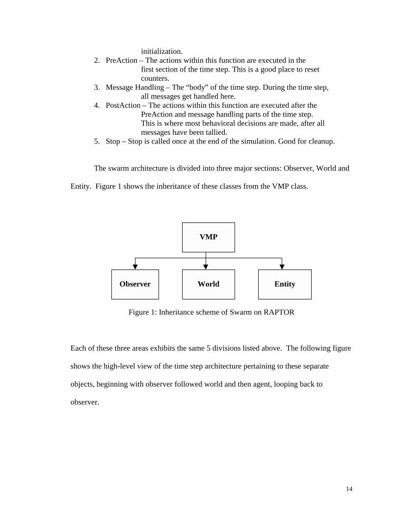
The swarm architecture is divided into three major sections: Observer, World and

Entity. Figure 1 shows the inheritance of these classes from the VMP class.

Figure 1: Inheritance scheme of Swarm on RAPTOR

Each of these three areas exhibits the same 5 divisions listed above. The following figure

shows the high-level view of the time step architecture pertaining to these separate

objects, beginning with observer followed world and then agent, looping back to

observer.

VMP

Observer

World

Entity

15

Figure 2: High-level view of time step architecture within swarm

These objects all interact with each other by passing messages of certain types.

There are two overall kinds of messages – swarm and RAPTOR. RAPTOR messages

contain a sender address and are manipulated via the RAPTOR message-passing engine.

Swarm messages are simply types or data and are sent directly to the qualifying nodes.

During the following descriptions of the objects, I will also discuss the types of messages

associated with each.

Agent

World

Agent

PostAction()

Body()

Body()

PreAction()

PostAction()

PreAction()

Body()

PostAction()

Observer Body()

PostAction()

PreAction()

Observer PreAction()Body()

PostAction()

PreAction()

Time Step n

PreAction()

16

4.2 Observer

The observer acts as an agent that is registered with the world but cannot be seen.

It acts as the interface between the user and the simulation. The observer queries the

world and the entities for information. It then outputs this information to the simulation

user. It can be output in any format the user wishes just by modifying the observer code.

The observer deals with query and status messages. It has two types of query messages:

one that is a RAPTOR message that goes to the world, and another swarm message that

goes to the agents. When the objects receive these messages they respond with status

messages of their own back to the observer. The observer queries the swarm entities

based on the observable information types listed below.

Observable Information Types sent to Entities: 1. NO_INFO 2. ENTITY_POSITIONS_INFO 3. BATTERY_LEVEL_INFO 4. REACHED_BY_BROADCAST_INFO 5. HAPPINESS_INFO

The observer can choose between any or all of these types to ask entities for by setting

certain bits in the message type. The observer is simply an invisible tool working in the

background to keep the user updated on the happenings of the simulation.

4.3 World The world acts as the moderator to the whole simulation. It keeps track of what

entities and observers are registered and also handles the wireless calculations. For

example, when an agent wishes to send a broadcast, it first sends a RAPTOR

TransmitMesssage with a designated signal strength or power to the world. The world

receives this message and calculates which agents are within the transmission radius. It

17

then forwards the TransmitMessage as a swarm ReceivedTransmissionMessage to the

appropriate entities. The world does keep track of the location of all entities but this does

not violate any rules, because it only uses this information for transmission calculations

and to relay entity data to the observer to display to the user.

All messages passed to the world are RAPTOR messages. Some of these

messages simply provide information, but some, like TransmitMessage and

FindMessage, get converted into swarm messages to forward to the group. The world

acts, in a sense, as the moderator and overseer to make sure everything flows properly.

4.4 Entity The entity object is what all types of agents are derived from. Figure 3 below

shows the general layout of the swarm agents.

Figure 3: Inheritance scheme of the entity structure

Entity

BasicAgent

TotalAgent

BehavioralAgent

FunctionalAgent

18

BasicAgent is inherited from Entity. BasicAgent contains the message handling

algorithms. It receives messages, determines their types, and then calls the appropriate

functions in either FunctionalAgent or BehavioralAgent. Inherited from BasicAgent are

FunctionalAgent and BehavioralAgent. These are separated for extensibility and

interchangeability. The functional side deals with the amount of power that is required to

perform certain tasks, such as moving, transmitting, and listening. The behavioral side

makes the decisions on when and where to move or transmit, and then calls the functions

on the functional object.

This is an ideal scenario for multiple inheritance, as the complete agent comes

together as a combination of the two sides. The user is then able to choose different

behaviors and functionalities. For example, the user could decide to test a disperse

behavior with different batteries which contain different powers, or vise versa, the user

can test different behaviors on the same battery model.

The division of swarm into these three areas works well with the extensibility of

the entire simulator. New features and models can be added and removed fairly

painlessly due to the object-oriented nature of the architecture. The disperse agent was

slipped right into this structure by simply deriving a disperse behavior and a disperse

functionality agent classes. Overall, the RAPTOR environment provides an excellent

framework to create a more realistic swarm simulator.

19

5 Disperse Primitive This chapter goes into more detail describing the disperse primitive in general. It then talks about the disperse on Santa Fe before discussing the newly implemented disperse on RAPTOR.

The disperse primitive describes the behavior of agents as they spread apart from

a clustered position or any position. This primitive would be useful in almost any swarm

application. Because, every time that you release some swarm robots, they will most

likely need to spread out before beginning their task. This chapter will discuss the

disperse primitive, how it was implemented in the Santa Fe simulator, and how it is now

implemented on the RAPTOR simulator.

5.1 Disperse Algorithm

Disperse takes a parameter, x, that represents the minimum distance away other

agents need to be for the given agent so be “dispersed.” It also needs to consider the cost

of its actions (transmitting, listening, moving) because in an actual environment, these

units will be dependent on a battery with limited power.

Devising a resource efficient disperse algorithm is not as simple as it may seem

on the surface. The easiest approach to this problem would rely on each agent querying a

server for the location of the agents surrounding it, and then deciding where to move

based on this information. This would work, but it is inconsistent with the notion of

swarm operating without a central server of any kind. So, the algorithm needs to obtain

any information it needs purely from other agents within its transmission area.

20

5.1.1 Random Dispersion Algorithm

One strategy is to use random motion. Agent A would move to a random location

and then transmit a message of a certain strength X. Agents that heard A’s transmission

would then respond to A with transmissions declaring that they were within X strength.

If A received any responses, it would then move to another random location and repeat

the same process. This would continue until no agents received any messages. The

swarm would then be in a satisfied or dispersed state.

This random algorithm is neither time efficient nor cost efficient. With the agents

moving and transmitting every time step, it, in fact, uses a great deal power. Another

problem arises when considering the message passing. Every agent will send out a

transmission each time step, so if there are 10 agents within a small area, each agent will

receive 9 other messages. What happens now? Do they all send out 9 responses (90

more transmissions)? And how do they know which response is for whom? These are all

issues that the researcher must resolve in the implementation of any disperse algorithm.

It would be beneficial to the algorithm if each agent had a specific address and name, but,

in an ideal swarm the agents would all be anonymous and would gain information only

by talking to their neighbors.

The agent could generate a random identification number upon release and then it

could append that number to the message that it sends out. This would still allow for

psuedo anonymity, whereby each node still has no finite name or ID. Using this method,

the receiving agent could discount any duplicate responses from the same agent. The

random disperse algorithm is neither cost efficient nor time efficient, but it does provide a

working method for comparisons with other algorithms.

21

5.1.2 Other Examples

A simple improvement upon the random method is an algorithm which

remembers the density of surrounding agents in time t-1, and then compares that with the

current density in time t. If the new density is greater, it then doubles the distance moved

and moves in the opposite direction.

More advanced dispersion algorithms could rely on information passed as data

within a transmission message. Agent A could broadcast a message saying “Hello, I’m

agent A.” Then agents within earshot could respond with, “Hi, I hear you, and I am agent

B.” Or, Agent A could transmit a message saying, “Hello, I am agent A. Who can hear

this and where are you?” The other agents could then respond with, “I am agent B and I

am to your left.” Agent A could then develop a sense of which agents are where and

decide the direction to move next based on that knowledge.

Already the trade-offs are becoming apparent. The simple hello message uses

little transmission power but it does not yield as much information and, in turn, will not

create as quick of an algorithm. To go even further, Agent A could ask the other agents,

who they have surrounding them. This would cost even more power but could lead to a

more time efficient approach. Other ideas entail an initial soft broadcast to gain an idea

of the density of agents nearby, followed by a stronger broadcast to gain an idea of the

density of agents further away.

An interesting approach lets each agent record where all the agents surrounding it

are located and assigns itself a random position. It then passes this dynamic area grid to

the other agents, which compile that with their own data and pass it along further. The

goal here is for each agent to have a complete area mapping of all the other agents

22

without moving. Theoretically, they could then all communicate with each other on

where to move and resolve a movement process that would immediately satisfy all units

being happily dispersed. Besides being inherently complex, this method would also

require significant storage capacity on the physical agents.

Yet another tactic is to divide the world into distinct areas and then move the

agents between these areas until each area is happily dispersed. The next step would then

require the programmer to create larger areas and repeat the same steps. The goal being

to keep dispersing larger and larger regions until the final dispersed state is reached

[Evans 2000].

There are many other methods that can be used to solve the requirements of a

disperse primitive. They all have to take into account the same trade-offs between power

consumed and time to completion. The next sections will discuss what type of disperse

method was used in each simulator.

5.2 Disperse on the Santa Fe Simulator

The Santa Fe simulator’s disperse primitive starts all agents together in one

cluster, shown in Figure 4. It then traverses through the algorithm until all agents are in a

satisfied state. The happiness of a unit is determined by the density of other units

surrounding it. So, if the simulated world is thought of as a grid of squares which are

either occupied or not, an agent is happy if it has no neighbors in its adjacent eight

squares. The simulation ends when all agents are in the happy state shown in Figure 5.

23

Figure 4: Screenshot of initial agent cluster in Santa Fe simulator

Figure 5: Screenshot of dispersed agents in the Santa Fe simulator

24

The disperse primitive which used the Santa Fe simulator was an N-Square away

algorithm. University of Virginia undergraduate Ryan Persaud originally developed this

algorithm. The N-Square away algorithm divides each possible move of an agent into a

grid of squares. It then weights each square based on the number of agents that can be

reached in N moves from the agent’s current position. The further away the agent is, the

less it affects the final weighting of the square [Persaud 2001].

2 3 4 1 Agent 5 8 7 6

Figure 6: N-square away grid [Persaud 2001]

Figure 6 above shows this movement grid. The agent would then make the

decision to move based on the lowest valued square. For example, in Figure 6, the agent

would choose to move one place to the left and then reassess its status. An interesting

side effect of this algorithm occurs when two agents are separated from the rest of the

group and continue to rotate around each other, thus the process never terminates

[Persaud 2001].

The algorithms that are implemented on the Santa Fe simulator consist of a

random movement and a 2-square away behavior. The user has the ability to determine

how many random agents and how many 2-square agents they want in the simulation.

Though there is no actual measurement of power consumption it is assumed that the

“smart” agents use more power whereas the random agents do not use as much.

25

Percent Simple Agents Percent Smart Agents Time to Completion 100 0 675 75 25 550 25 75 150 0 100 65

Figure 7: Table of Sample data from Santa Fe simulator

After looking at Figure 7, it is clear to see that the smart agents can achieve a

dispersed state significantly quicker than the simple agents. It is a nice feature to be able

to determine how many of each agent is needed because it allows for some variance in

the trade-off values of the user.

This works excellently in practice, however, theoretically, it violates one

requirement of swarm programming. To gather the information regarding how many

agents are in each direction, the program queries the central simulator for location data.

This required a new algorithm to be developed, either an algorithm to determine

the area data without querying a central server, or a completely new method. After

discussing this task with other swarm researchers, I decided to implement the new swarm

disperse on the new swarm-capable RAPTOR simulator.

5.3 Disperse on the RAPTOR Simulator

Creating a behavior in swarm on RAPTOR was fairly straightforward. As Figure

8 shows, I used the existing the system functionality and inherited a new disperse agent

behavior functionality. I then inherited a new total disperse agent from both the system

and behavior sides.

26

BasicAgent

|+---------+---------+| |

PowerAgent DisperseAgent| |+---------+---------+

|PowerDisperseAgent

Figure 8: Inheritance sketch [Hogye 2002]

In order to obtain the desired effects, I added some functionality and created new

message types. First, I needed a way for the simulator to end once all the agents were in

the dispersed state. So, I created a new status message that would be queried each time

step by the observer. The message, HappinessMessage, is almost identical to

BatteryLevelMessage. The HappinessMessage contains one data member called state,

which is Boolean and simply tells if the specific entity is happy or not. The observer

receives this information for each entity in each time step and cycles through the results.

If it goes three consecutive complete time steps without receiving any unhappy messages

it exits and the program terminates. Three was the number assigned here because it

seemed like a valid number of time steps to wait to ensure a proper dispersion. This

number can be easily modified by the user, based on their individual preferences.

Another problem I encountered was the method taken by the behavior side agent

to determine happiness. I programmed the agent to set its happiness to true in the start

function and then to change the value to false if it received a

ReceivedTransmissionMessage. The problem arose once an agent’s happiness would be

set to false; there was no mechanism to return the value to true. I decided to implement

another counter (hcount) that would count the time steps that pass without the agent

27

receiving a message. If the agent makes it four consecutive time steps, it again becomes

a happy agent. The agent will not be moving during these four steps, so it ensures that it

is in an empty area and not just a random pocket.

I also needed a way for the agents to send a message asking who could hear them.

This could be done using a simple TransmitMessage and all recipients of the

ReceivedTransmissionMessage could just reply with another TransmitMessage. This

would cause great confusion, however, as each agent would receive multiple

ReceivedTransmissionMessages, and would not know which were directed as a reply to

them or a reply to others, or which were queries that they needed to respond to. To avoid

this chaos, I created a new message set, FindMessage and FoundMessage. These are

very similar to TransmitMessage and ReceivedTransmissionMessage in that

FindMessage is sent to the world and the world then determines who can hear the

message and forwards the FoundMessage to the qualifying agents. These messages do

not have a frequency or data components; they are just made up of a power setting.

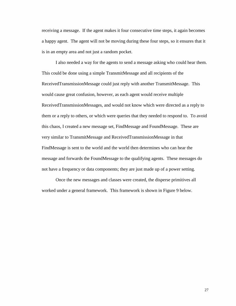
Once the new messages and classes were created, the disperse primitives all

worked under a general framework. This framework is shown in Figure 9 below.

28

Figure 9: Flow chart of general disperse framework

This framework describes the way all of my disperse algorithms work. In step 1, the

agent creates and sends a FindMessage to determine who is within the transmit strength

radius. It then sends this message to the World. The World converts it into a

FoundMessage to send to all agents close enough (step 2). In step 3, an agent receives

the FoundMessage and creates a TransmitMessage to send to the world as a reply to the

FoundMessage. No matter how many FoundMesssages the agent receives it only sends

one TransmitMessage. This avoids multiple responses being sent and the agents not

knowing what was meant for them. It still works because the agents send the

TransmitMessage at the same signal strength as the FoundMessage, so everyone who sent

a FindMessage will hear the same ReceivedTransmissionMessage and can count it as

their own. In step 4 the world simply converts the TransmitMessage into a

ReceivedTransmissionMessage and sends to the agents that are within the radius. Step 5

Start

1 Agent A

sends FindMsg

2 World recvs

FindMsg, sends FoundMsg to

Agents 3

Agent recvs FoundMsg

Sends only 1 TransmitMsg

4 World recvs

TransmitMsg, sends

RecvTranMsg to Agents

5 Agent A recvs RecvTranMsg.

counts msgs, and makes behavior decision, sets

Happiness

29

contains the behavior of each primitive. In each, the agent counts how many other agents

have responded and then decides what to do, depending on what type of agent it is, before

repeating the process.

I first implemented a purely random disperse agent. This agent moves every time

step regardless of how many messages it received. If no messages are received it sets its

happiness state to true. The simulation ends when all the agents reach a state where they

are all happy at the same time. This behavior is shown with the state machine in Figure

10 below.

Figure 10: Decision chart of a Random Disperse Agent

After I got the random disperse working as a comparison tool, I implemented an

N-threshold density algorithm. In this algorithm, the agent decides whether or not it

moves based on a threshold of messages received. If it is a 2-threshold implementation,

the agent will only move if it receives 2 or more messages in that time step. The

happiness state is the same in this implementation as in the random version. The goal is

to reduce the amount of battery power used in reaching a dispersed state. Using this

method, the agents that are in the densest areas use their power to move, while the agents

Msg = FindMessage

Transmit(msg);

m_Happiness = false;Move();

m_Happiness = true; Move(); If no RecvTranMsgs received

If RecvTranMsgs received

30

in less dense areas save power and wait for new developments. The following code is

what guides the behavior of the N-threshold dispersion algorithm:

void DisperseDAgent::behavior_post_action() { if ((m_msg_count >= m_threshold) && (!m_happiness)) m_moving = true; //If the agent received enough nodes to warrant a

//move dependant upon the algortithm specified if (m_moving) { double x = (((((double) rand()) / RAND_MAX) - 0.5) ); //Generates random direction double y = (((((double) rand()) / RAND_MAX) - 0.5) ); move(Position(x,y)); } if (hcount >3) //If agent has gone three time steps without receiving a m_happiness = true; //ReceivedTransmissionMessage set Happiness state to true else hcount++; //Increment the number of steps gone without recv a msg. m_msg_count = 0; //Reset message counter }

When picking N, it is dependent on the users views of the trade-offs. Obviously a

high N will use the least amount of power, while low values will reach a better dispersed

state. One problem with this algorithm is that it can sometimes run indefinitely. For

example, this happens when a threshold of 2 is chosen and an agent receives one message

from other agents. It never moves because one is less than two, yet, it never switches to

happy because it is continually receiving messages. Researchers who wish to have the

swarm relatively spread out without much battery usage and in a short amount of time

will implement this type of algorithm.

31

It is interesting to note that a modified random algorithm can be produced if you

set the threshold to 0. In this algorithm, the agent does not move if it is already happy

which is the only difference from the purely random method. This seems like it should

be one step up from the pure random implementation due to not using as much power.

The actual results of selected variations of this algorithm will be discussed in depth in the

results chapter.

The final step in the creation of a dispersion primitive was to create a readable

display to keep things interesting. Mike Hogye wrote a simple program to take a text

output of a simulation and display it using OpenGL and GLUT. I used this display

program to create a simple display of the swarm states of disperse.

Disperse runs on the RAPTOR simulator without having to use a central server to

gather area location. There are numerous other experiments to be tried and developed on

this simulator now that this bridge has been crossed. The implementation is

straightforward enough to easily facilitate new research into this area of Computer

Science.

32

6 Results

Since this is the not only the first time that disperse has been tested in the

RAPTOR simulator, but also the first time any swarm application has been implemented

in RAPTOR, these results relied on certain assumptions and research decisions. These

preliminary results discuss the power and dispersion efficiencies of a variety of different

dispersion algorithms.

6.1 Random Algorithm The first algorithm that I created and tested was the purely random

implementation. This algorithm had its agents move every time step regardless whether

they were happy or not. Figure 11 shows how the Random Algorithm responded to the

strength of the transmission. Since the state of dispersion depends on how many

messages the agent can hear, the stronger the transmission the longer it takes the agents to

become reasonably dispersed.

Random Algorithm

0

50

100

150

200

250

300

0 1 2 3 4 5 6 7 8

Disperse Distance Threshold

Tim

e to

Rea

sona

ble*

C

ompl

etio

n

Figure 11: Random Algorithm – Disperse Distance vs Time to Complete

33

Because some algorithms will never reach a completely dispersed state and will continue

indefinitely, I had to define a reasonable completion time. This was obtained by stopping

the simulation once the agents were receiving no more than 1 message instead of 0

messages. Figure 12 shows the how the same random algorithm responds to an

increasing number of agents. As the agents get denser and denser it is inherent that the

time it takes them to disperse increases significantly.

Random Algorithm

0

10

20

30

40

50

0 200 400 600 800 1000 1200

Number of Agents (Density)

Tim

e to

Com

plet

ion

Figure 12: Random Algorithm- Number of agents vs time to completion

6.2 0-Threshold Algorithm

The 0-Threshold algorithm is basically a modification of the random

implementation. Now, instead of the agents moving every time, if they are happy, they do

not move. The following figures are the same as above only show how the 0-threshold

algorithm responded to a higher transmission power and more agents respectively.

34

0 Threshold Algorithm

020406080

100120140160

0 1 2 3 4 5 6 7 8

Disperse Distance Threshold

Tim

e to

Rea

sona

ble*

C

ompl

etio

n

Figure 13: 0-Threshold Algorithm – Disperse distance vs time to completion

0-Threshold Algorithm

0

5

10

15

20

25

0 200 400 600 800 1000 1200

Number of Agents (Density)

Tim

e to

Com

plet

ion

Figure 14: 0-Threshold Algorithm- No. of Agents vs Time to Completion

6.3 1-Threshold Algorithm

The 1-threshold algorithm is just one step further into N-threshold family of

algorithms. For the purpose of succinctness, this report will only highlight the random,

0-threshold, and 1-threshold individually. The other algorithms will be considered in the

35

comparison section. The following figures show the reaction of the 1-threshold

algorithm to the transmission strength and the number of agents.

1 Threshold Algorithm

0

20

40

60

80

100

120

0 1 2 3 4 5 6 7 8

Desnity Distance Threshold

Tim

e to

Rea

sona

ble*

C

ompl

etio

n

Figure 15: 1-Threshold Algorithm – Density distance vs time to completion

1-Threshold Algorithm

0

3

6

9

12

15

18

0 200 400 600 800 1000 1200

Number of Agents (Density)

Tim

e to

Com

plet

ion

Figure 16: 1-Threshold Algorithm – No. of agents vs time to completion

36

6.4 Comparison of Algorithms

These algorithms mostly behave similar to the given variable alterations above.

Figures 17 and 18 show a compilation of the data for all the algorithms.

AVERAGE TIME TO COMPLETION

Transmission Strength Random 0-Threshold 1-Threshold .01 9 11 11 .05 9 17 11 .1 16 22 13 .2 16 22 13 .4 25 28 17 .5 26 32 23 1 38 48 23

1.5 38 69 40 2 39 77 42 3 92 94 50 4 193 113 55 7 286 148 105

Figure 17: Table of time to completion based on transmission strength

Notice that the higher the threshold gets, the less varying the time becomes. For

Example, the 0 and 1-thresholds are not as quick as the random implementation for the

extremely small strengths and they are not as slow as random for the extremely powerful

strengths.

37

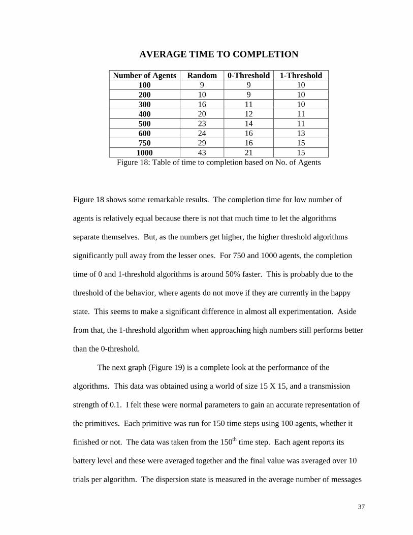
AVERAGE TIME TO COMPLETION

Number of Agents Random 0-Threshold 1-Threshold 100 9 9 10 200 10 9 10 300 16 11 10 400 20 12 11 500 23 14 11 600 24 16 13 750 29 16 15 1000 43 21 15

Figure 18: Table of time to completion based on No. of Agents

Figure 18 shows some remarkable results. The completion time for low number of

agents is relatively equal because there is not that much time to let the algorithms

separate themselves. But, as the numbers get higher, the higher threshold algorithms

significantly pull away from the lesser ones. For 750 and 1000 agents, the completion

time of 0 and 1-threshold algorithms is around 50% faster. This is probably due to the

threshold of the behavior, where agents do not move if they are currently in the happy

state. This seems to make a significant difference in almost all experimentation. Aside

from that, the 1-threshold algorithm when approaching high numbers still performs better

than the 0-threshold.

The next graph (Figure 19) is a complete look at the performance of the

algorithms. This data was obtained using a world of size 15 X 15, and a transmission

strength of 0.1. I felt these were normal parameters to gain an accurate representation of

the primitives. Each primitive was run for 150 time steps using 100 agents, whether it

finished or not. The data was taken from the 150th time step. Each agent reports its

battery level and these were averaged together and the final value was averaged over 10

trials per algorithm. The dispersion state is measured in the average number of messages

38

received in the final time step. So, if the average is 0, then the swarm had already

reached complete dispersion.

Algorithms: Battery Level and Dispersion Level

00.20.40.60.8

11.21.41.6

Rando

m

0-Thre

shold

1-Thre

shold

2-Thre

shold

3-Thre

shold

4-Thre

shold

Type of Algorithm

Aver

age

# of

Mes

sage

s R

ecei

ved

00.050.10.150.20.250.30.350.40.450.5

Avg.

Bat

tery

Lev

el L

eft i

DispersionBattery Level

Figure 19: Algorithms: Battery Level and Dispersion Level

There are several interesting results displayed in Figure 19. The fact that the 0-

threshold algorithm does not have a fully dispersed state is quite interesting. This was an

unexpected result and is interesting to look at. In the code, as soon as an agent receives a

ReceivedTransmissionMessage the happiness gets set to false. It then is required to go

three consecutive time steps without getting another message before the value gets set

back to true. The reason for the agents that are not dispersed yet by 150 time steps has to

be attributed to them being repeatedly stuck in the two time steps where they can receive

no messages yet still be unhappy.

After 150 time steps, the Random primitive and the 0-threshold primitive both

have run their agents batteries dead. The interesting thing to note is the trade-off between

39

power and efficiency ceases to be a trade-off at a certain point. At around the 2-threshold

algorithm, the battery level starts to level out while the dispersion state gets worse and

worse. For example, the only large difference between the 4-threshold disperse and the

2-threshold disperse is that the final dispersion state is much worse. That is not a trade-

off at all!

These results are just a small chip into the abundance of research that still needs

to be done in swarm computing. These do show, however, a good deal of information

about the general characteristics of the dispersion primitive.

40

7 Conclusion

7.1 Summary

This project looked into swarm programming’s building blocks called primitives.

It specifically performed research on the disperse primitive. The disperse primitive

guides a group of individual agents from a clustered state to a dispersed state, where it

satisfies some constraint d. In completion, no agents can be within d distance of each

other. The key to any swarm primitive is getting it to behave properly without the use of

a central computer. Disperse can be implemented in a variety of manners while still

holding to this constraint.

The most basic of these approaches is the random disperse. This method consists

of agents moving in a random direction every time step until the entire swarm reaches a

dispersed state. The only constraint on this algorithm is that there is not another agent in

the chosen direction. This project implemented and analyzed a random disperse on the

RAPTOR simulator.

Implementing swarm primitives involves many trade-offs. One important trade-

off in this type of research is the power consumed versus time to completion trade off.

The random disperse uses a great deal of power, and it is also fairly slow. This project

also looked at an N-threshold density primitive, which is based on the notion of

qualifying trade-offs. If the user does not mind having a final state with less than a

perfect dispersal, they can pick how perfect they need it to be, and hopefully gain some

advantages in battery power. These algorithms work by specifying a threshold, which is

the maximum number of messages received by an agent. Beyond this threshold, the

41

agent will be instructed to move to a new location, but below it, the agent will stay where

it is. This, in theory, will allow power to be used by the agents in high-density areas

while the outlying agents can save some power while they wait to see where the swarm

moves.

The N-threshold algorithms did save significant amounts of battery power when

compared to the random primitives. They also reached their individually assigned

satisfied state slower than the random ones. The N-threshold algorithms are only useful

up to a small N. After a certain N, the battery level will level off while the dispersion

continually gets worse.

7.2 Interpretation

The implementation of the random disperse primitive was crucial in the ability to

test any of the other primitives. The N-threshold algorithm performed slightly better than

expected when compared against the others. Certainly the 1-threshold version was

clearly a much better choice than the random implementation in both power consumption

and efficiency. Extending the data beyond the 3-threshold algorithms was also effective

in showing how the battery level exhibits a logarithmic behavior as it approaches an

horizontal asymptote. This makes sense when thinking about the number of agents, if the

experiments were run again with a higher number of agents, it would probably push the N

of N-threshold to a higher number before leveling off.

The 0-threshold algorithm is only beneficial to the random implementation when

there is an extreme value -- either a lot of agents or high broadcasting power. 1-threshold

seems to be a good, safe choice for a balance of the trade-offs. These numbers would all

vary, of course, by altering the environment in which they were tested.

42

One of the key results of this project was getting some basic primitives working

on the RAPTOR simulator. Now that there is a working framework of swarm

technologies available on the RAPTOR simulator, it will be easier to do new and better

research. Regardless of the actual simulator, it was a significant step in swarm research

because we entered into a simulation that does not use a central server as a mainstay in

the primitive. Having a disperse algorithm that can be manipulated and experimented

with, while still only utilizing the other agents is a move towards the future, towards

more realistic simulations and eventually to widespread swarm application usage.

7.3 Recommendations

There are many more angles that new research could take on. Having the ability

to change variables and to reach different results based on the implementation can lead to

some great things. A new research project may be to build a swarm application

developer, where the user specifies what variables are important to them, and then the

software automatically generates a swarm primitive, which meets their needs the best.

Another feature that could go along with the automated personalized primitive

builder could be the ability to pick and choose how many of what agents would be

needed. This would involve some sort of selection algorithm with weights for each

primitive and a target weight that would try to be met.

On a more basic note, there is plenty of room for developing more dispersion

primitives and testing them against the ones developed in this project. I mentioned a few

ideas earlier in the paper, and there so many other ways to go about this problem that

there will always be more research available in finding new algorithms.

43

Optimization is always necessary in any stage of research and development.

Whether this is to optimize the code or the simulator to handle extraordinarily large node

counts, each would be helpful to the common goal.

In particular, it would be interesting to see a new primitive where the agents have

a limited memory. They would use this memory to remember the direction they most

recently moved and the density of agents in that previous location. Upon arriving in a

new position, the agent would figure out the density there, and if it was more than where

the agent came from it would move in the opposite direction it just moved and twice as

far. This approach seems that it would be more and more beneficial with the more units

that it was implemented on.

Overall, this research suggests numerous more research opportunities. This

research has provided a solid foundation for more in-depth and advanced research to be

done on top of it. It is an accomplishment to have working swarm primitives using a

communication algorithm based solely on information from neighboring swarm units.

This provides another forward step towards more realistic swarm simulations, which will

lead to a better future of the modern technological world.

44

Bibliography 1. Broch, Josh, David A. Maltz, David B. Johnson, Yih-Chun Hu, and Jorjeta Jetcheva.

(1998). “A Performance Comparison of Multi-Hop Wireless Ad Hoc Network Routing Protocols.” Proceedings of the Fourth Annual ACM/IEEE International Conference on Mobile Computing and Networking (MobiCom 1998), ACM.

2. Hill, J., P. Boundadonna, and D. Culler. (2001) “Active Message Communication for Tiny Network Sensors.” Submitted to INFOCOM 2001.

3. Chen, Benjie, Kyle Jamieson, Hari Balakrishnan, and Robert Morris. (2001). “Span:

An Energy-Efficient Coordination Algorithm for Topology Maintenance in Ad Hoc Wireless Networks.” Proceedings of the Seventh Annual ACM/IEEE International Conference on Mobile Computing and Networking (MobiCom 2001).

4. Daniels, Marcus. (1999). “Integrating Simulation Technologies With Swarm.”

Submitted to the Swarm Programming Group at www.swarm.org. 5. Daniels, Marcus. (2000). “Writing Fast Models in Swarm.” Submitted to the Swarm

Programming Group at www.swarm.org. 6. Li, Qun, Javed Aslam, and Daniela Rus. (2001). “Online Power-aware Routing in

Wireless Ad-hoc Networks.” Proceedings of the Seventh Annual ACM/IEEE International Conference on Mobile Computing and Networking (MobiCom 2001).

7. Swarm Development Group. (2000). “Brief Overview of Swarm.” www.swarm.org. 8. Swarm Development Group. (2001). “Getting Started with Swarm.”

www.swarm.org. 9. Loizeaux, John David. (2001). “Building the Swarm: A Review of Three Areas

Necessary for Swarm Computing.” Senior Thesis, University of Virginia. 10. Persaud, Ryan K. (2001). “Investigating the Fundementals of Swarm Computing.”

Senior Thesis, University of Virginia. 11. Tennenhouse, David. (2000). “Embedding the Internet: Proactive Computing”.

Communications of the ACM, 43, 44-50. 12. Evans, David. (2000). “Programming the Swarm.” 13. Werger, Barry Brian, and Maja Mataric. (2000). “From Insect to Internet: Situated

45

Control for Networked Robot Teams.” Annals of Mathematics and Artificial Intelligence, 31:1-4, pp. 173-198, 2001.

14. Harold Abelson, Don Allen, Daniel Coore, Chris Hanson, George Homsy, Thomas F. Knight, Radhika Nagpal, Erik Rauch, Gerald Jay Sussman and Ron Weiss.

(2000). "Amorphous Computing". Communications of the ACM, Volume 43 , Issue 5 2000.

15. Box, Paul. “Swarm-based assistantships at Utah State.” paulbox@cc.usu.edu (22 Feb. 2002).

16. Wantanabe, Toshiro. “Hello.” toshiro@urban.tutrp.tut.ac.jp (25 Jan. 2002).

16. Schreiber, Darren. “Swarm in the news -> ‘The sims take on Al Queda’ dschreib@ucla.edu (3 Nov. 2001).

17. McEachron, Errol. (2002). “A System for Synthesizing Swarm Applications.”

Unpublished. UVA BS Thesis, May 2002. 18. Hogye, Mike. (2002). “Realizing Fine-grained Trade-offs in Swarm Systems.”

Unpublished. UVA BS Thesis, May 2002.

19. Koenig, Sven and Yaxin Liu. (2001). “Terrain Coverage with And Robots: A Simulation Study” Agents 2001: 600-607.

20. Koenig, Sven, Boleslaw K. Szymanski, Yaxin Liu. (2001). Efficient and inefficient ant

coverage methods. Annals of Mathematics and Artificial Intelligence 31(1-4): 41-76.

46

Appendix A - Disperse On Raptor Code Listings BasicAgent.h: #ifndef BASIC_AGENT_H#define BASIC_AGENT_H

#include "Entity.h"#include "ReceivedTransmissionMessage.h"#include "QueryMessage.h"#include "Position.h"

#include "FoundMessage.h"

class BasicAgent : public Entity{

public:BasicAgent(int world_addr, const Gate &world_gate, double sensor_sensitivity);

double get_sensor_sensitivity() const;

protected:// Behavior.virtual void behavior_start() = 0;virtual void behavior_pre_action() = 0;virtual void behavior_post_action() = 0;virtual void behavior_stop() = 0;

virtual void behavior_received_transmission(ReceivedTransmissionMessage *msg) = 0;

virtual void behavior_answer_query(int observer_addr, QueryMessage *msg) = 0;

virtual void behavior_found(FoundMessage *msg) = 0;

// Functionality systems.virtual void systems_start() = 0;virtual void systems_stop() = 0;

virtual void move(const Position &position) = 0;virtual void transmit(const char *data, double power, double frequency) = 0;

virtual void find_message(double power)= 0;virtual void listen() = 0;

virtual bool is_listening() const = 0;virtual double get_battery_level() const = 0;

virtual double max_move_distance(double cost) const = 0;virtual double max_transmit_power(double cost, int length, double frequency) const

= 0;virtual int max_transmit_length(double cost, double power, double frequency) const

= 0;virtual double max_transmit_frequency(double cost, int length, double power) const

= 0;virtual int max_listen_time(double cost) const = 0;

virtual double move_cost(double distance) const = 0;virtual double transmit_cost(int length, double power, double frequency) const =

0;virtual double listen_cost() const = 0;

virtual void systems_answer_query(int observer_addr, QueryMessage *msg) = 0;

private:

47

BasicAgent(const BasicAgent &basic_agent);

void entity_start();void entity_pre_action();void entity_post_action();void entity_stop();

void handle_message(int sender_addr, Message *receive_msg);

double m_sensor_sensitivity;

};

#endif

48

BasicAgent.cpp: #include "BasicAgent.h"#include "BatteryLevelMessage.h"

#include "Debug.h"

BasicAgent::BasicAgent(int world_addr, const Gate &world_gate, double sensor_sensitivity): Entity(world_addr, world_gate), m_sensor_sensitivity(sensor_sensitivity)

{ }

double BasicAgent::get_sensor_sensitivity() const{

return m_sensor_sensitivity;}

void BasicAgent::entity_start(){

systems_start();behavior_start();

}

void BasicAgent::entity_pre_action(){

behavior_pre_action();}

void BasicAgent::handle_message(int sender_addr, Message *receive_msg){

switch (receive_msg->get_type()){

case RECEIVED_TRANSMISSION_MSG:

if (is_listening()){

behavior_received_transmission((ReceivedTransmissionMessage*) receive_msg);

}break;

case QUERY_MSG:systems_answer_query(sender_addr, (QueryMessage *) receive_msg);behavior_answer_query(sender_addr, (QueryMessage *) receive_msg);break;

case FOUND_MSG:

behavior_found((FoundMessage *) receive_msg);

break;

default:fprintf(DEBUG, "BasicAgent::handle_message - WARNING - don't

understand message type %d.\n", receive_msg->get_type());break;

}}

void BasicAgent::entity_post_action(){

behavior_post_action();}

void BasicAgent::entity_stop(){

behavior_stop();systems_stop();

}

49

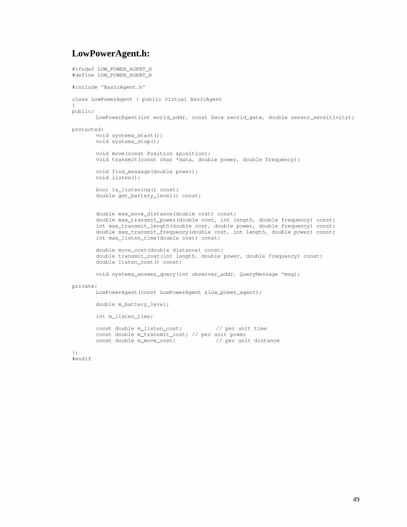
LowPowerAgent.h: #ifndef LOW_POWER_AGENT_H#define LOW_POWER_AGENT_H

#include "BasicAgent.h"

class LowPowerAgent : public virtual BasicAgent{public:

LowPowerAgent(int world_addr, const Gate &world_gate, double sensor_sensitivity);

protected:void systems_start();void systems_stop();

void move(const Position &position);void transmit(const char *data, double power, double frequency);

void find_message(double power);void listen();

bool is_listening() const;double get_battery_level() const;

double max_move_distance(double cost) const;double max_transmit_power(double cost, int length, double frequency) const;int max_transmit_length(double cost, double power, double frequency) const;double max_transmit_frequency(double cost, int length, double power) const;int max_listen_time(double cost) const;

double move_cost(double distance) const;double transmit_cost(int length, double power, double frequency) const;double listen_cost() const;

void systems_answer_query(int observer_addr, QueryMessage *msg);

private:LowPowerAgent(const LowPowerAgent &low_power_agent);

double m_battery_level;

int m_listen_time;

const double m_listen_cost; // per unit timeconst double m_transmit_cost; // per unit powerconst double m_move_cost; // per unit distance

};#endif

50

LowPowerAgent.cpp: #include "LowPowerAgent.h"#include "MoveEntityMessage.h"#include "TransmitMessage.h"#include "BatteryLevelMessage.h"#include "FindMessage.h"#include <float.h>#include "debug.h"

LowPowerAgent::LowPowerAgent(int world_addr, const Gate &world_gate, doublesensor_sensitivity)

: BasicAgent(world_addr, world_gate, sensor_sensitivity), m_listen_time(-1),m_listen_cost(0.005), m_transmit_cost(0.005), m_move_cost(0.005)

{add_observable_info_type(BATTERY_LEVEL_INFO);

}

void LowPowerAgent::systems_start(){

m_battery_level = 1.0;}

void LowPowerAgent::systems_stop(){

}

void LowPowerAgent::move(const Position &position){

double cost = move_cost(position.distance());if (m_battery_level >= cost){

Message *move_msg = new MoveEntityMessage(position);m_mailbox->send(get_world_handle(), &move_msg, sizeof(move_msg));m_battery_level -= cost;

}

if (m_battery_level == 0.0)fprintf(DEBUG, "move bat dead\n");

}

void LowPowerAgent::transmit(const char *data, double power, double frequency){

int length = strlen(data);double cost = transmit_cost(length, power, frequency);

if (m_battery_level < cost){

power = max_transmit_power(m_battery_level, length, frequency);m_battery_level = 0.0;

}else

{m_battery_level -= cost;

}

Message *transmit_msg = new TransmitMessage(data, power, frequency);m_mailbox->send(get_world_handle(), &transmit_msg, sizeof(transmit_msg));

if (m_battery_level == 0.0)fprintf(DEBUG, "Transmit bat dead\n");

}

51

void LowPowerAgent::find_message(double power){

Message *find_msg = new FindMessage(power);m_mailbox->send(get_world_handle(), &find_msg, sizeof(find_msg));

}

void LowPowerAgent::listen(){

double cost = listen_cost();if (m_battery_level >= cost){

m_listen_time = m_mailbox->getTime();m_battery_level -= cost;

}

if (m_battery_level == 0.0)fprintf(DEBUG, "Listen bat dead\n");

}

bool LowPowerAgent::is_listening() const{

return (m_listen_time == m_mailbox->getTime());}

double LowPowerAgent::get_battery_level() const{

return m_battery_level;}

double LowPowerAgent::max_move_distance(double cost) const{

return (cost / m_move_cost);}

double LowPowerAgent::max_transmit_power(double cost, int length, double frequency) const{

return (cost / (m_transmit_cost * length));}

int LowPowerAgent::max_transmit_length(double cost, double power, double frequency) const{

return ((int) (cost / (m_transmit_cost * power)));}

double LowPowerAgent::max_transmit_frequency(double cost, int length, double power) const{

return DBL_MAX;}

int LowPowerAgent::max_listen_time(double cost) const{

return ((int) (cost / m_listen_cost));}

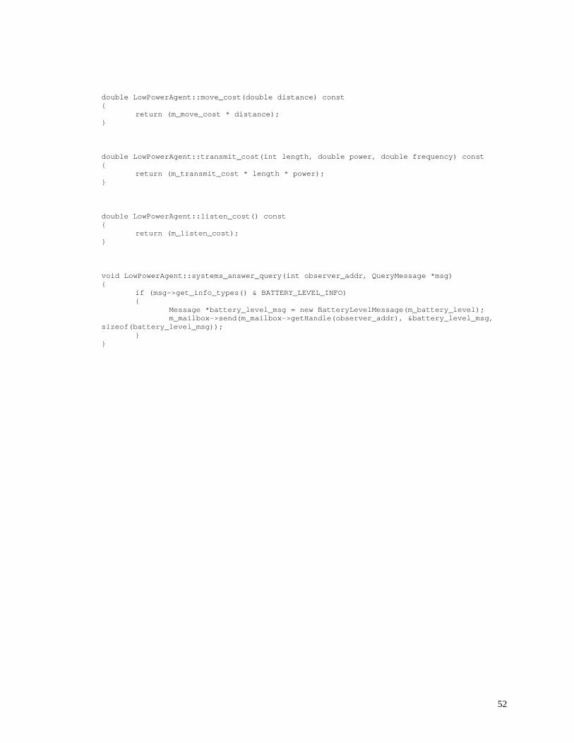
52

double LowPowerAgent::move_cost(double distance) const{

return (m_move_cost * distance);}

double LowPowerAgent::transmit_cost(int length, double power, double frequency) const{

return (m_transmit_cost * length * power);}

double LowPowerAgent::listen_cost() const{

return (m_listen_cost);}

void LowPowerAgent::systems_answer_query(int observer_addr, QueryMessage *msg){

if (msg->get_info_types() & BATTERY_LEVEL_INFO){

Message *battery_level_msg = new BatteryLevelMessage(m_battery_level);m_mailbox->send(m_mailbox->getHandle(observer_addr), &battery_level_msg,

sizeof(battery_level_msg));}

}

53

DisperseDAgent.h: #ifndef DISPERSE_D_AGENT_H#define DISPERSE_D_AGENT_H

#include "BasicAgent.h"#include "stdio.h"

class DisperseDAgent : public virtual BasicAgent{

public:DisperseDAgent(int world_addr, const Gate &world_gate, double sensor_sensitivity);

protected:

void behavior_start();void behavior_pre_action();void behavior_post_action();void behavior_stop();

void behavior_received_transmission(ReceivedTransmissionMessage *msg);void behavior_found(FoundMessage *msg);void behavior_answer_query(int observer_addr, QueryMessage *msg);

private:

DisperseDAgent(const DisperseDAgent &disperse_agent);

const unsigned int m_random_seed;bool m_reached_by_broadcast;bool m_happiness;bool found_gotten;bool moving;int hcount;int msg_count;FILE *m_out;

};

54

DisperseDAgent.cpp: #include "DisperseDAgent.h"#include "ReachedByBroadcastMessage.h"#include "HappinessMessage.h"#include <string.h>#include "Debug.h"

DisperseDAgent::DisperseDAgent(int world_addr, const Gate &world_gate, doublesensor_sensitivity)

: BasicAgent(world_addr, world_gate, sensor_sensitivity), m_random_seed(rand()),m_out(stdout){

add_observable_info_type(REACHED_BY_BROADCAST_INFO);add_observable_info_type(HAPPINESS_INFO);

}

void DisperseDAgent::behavior_start(){

m_reached_by_broadcast = false;m_happiness = true;hcount = 0;msg_count = 0;srand(m_random_seed);

}

void DisperseDAgent::behavior_pre_action(){

found_gotten = false;moving = false;listen();msg_count = 0;find_message(0.01);

}

void DisperseDAgent::behavior_received_transmission(ReceivedTransmissionMessage *msg){

msg_count++;hcount = 0;

m_happiness = false;

}

void DisperseDAgent::behavior_found(FoundMessage *msg){

if (!found_gotten){

transmit("", 0.01, 1.0);found_gotten = true;

}}

void DisperseDAgent::behavior_answer_query(int observer_addr, QueryMessage *msg){

if (msg->get_info_types() & REACHED_BY_BROADCAST_INFO){

Message *reached_by_broadcast_msg = newReachedByBroadcastMessage(m_reached_by_broadcast);

m_mailbox->send(m_mailbox->getHandle(observer_addr),&reached_by_broadcast_msg, sizeof(reached_by_broadcast_msg));

55

}

if (msg->get_info_types() & HAPPINESS_INFO){

Message *happiness_msg = new HappinessMessage(m_happiness);m_mailbox->send(m_mailbox->getHandle(observer_addr), &happiness_msg,

sizeof(happiness_msg));}

}

void DisperseDAgent::behavior_post_action(){

if ((msg_count >= 1))moving = true;

if (moving){

double x = (((((double) rand()) / RAND_MAX) - 0.5) *15);double y = (((((double) rand()) / RAND_MAX) - 0.5) *15);

move(Position(x,y));}

if (hcount >3)m_happiness = true;

elsehcount++;

msg_count = 0;

}

56

LowPowerDisperseDAgent.h #ifndef LOW_POWER_DISPERSE_AGENT_H#define LOW_POWER_DISPERSE_AGENT_H

#include "LowPowerAgent.h"#include "DisperseAgent.h"

class LowPowerDisperseAgent : public LowPowerAgent, public DisperseAgent{

public:LowPowerDisperseAgent(int world_addr, const Gate &world_gate, double

sensor_sensitivity);

};

#endif

LowPowerDisperseDAgent.cpp: #include "LowPowerDisperseDAgent.h"

LowPowerDisperseDAgent::LowPowerDisperseDAgent(int world_addr, const Gate &world_gate,

double sensor_sensitivity): BasicAgent(world_addr, world_gate, sensor_sensitivity),LowPowerAgent(world_addr, world_gate, sensor_sensitivity),DisperseDAgent(world_addr, world_gate, sensor_sensitivity)

{ }

57

BasicObserver.h: #ifndef BASIC_OBSERVER_H#define BASIC_OBSERVER_H

#include "Observer.h"#include "BasicEntitySnapshot.h"#include "EntityPositionMessage.h"#include "ReachedByBroadcastMessage.h"#include "BatteryLevelMessage.h"#include "ObservableDescription.h"#include "HappinessMessage.h"

#include <stdio.h>

class BasicObserver : public Observer{

public:BasicObserver(int num_entities);virtual ~BasicObserver();

void register_world(int addr, ObservableInfoType info_types);void register_entity(int addr, ObservableInfoType info_types);

private:BasicObserver(const BasicObserver &observer);

void observer_start();void observer_pre_action();void observer_post_action();void observer_stop();

void handle_message(int sender_addr, Message *receive_msg);

void observe_entity_position(EntityPositionMessage *msg);void observe_reached_by_broadcast(int entity_addr, ReachedByBroadcastMessage

*msg);void observe_battery_level(int entity_addr, BatteryLevelMessage *msg);void observe_happiness(int entity_addr, HappinessMessage *msg);

void sort_snapshots();BasicEntitySnapshot *get_snapshot(int addr);

const int m_num_entities;int m_entities_registered;bool m_world_registered;ObservableDescription m_world_description;ObservableDescription *m_entity_descriptions;BasicEntitySnapshot *m_entity_snapshots;FILE *m_out;int m_kill_count;int timer;

};

#endif

58

BasicObserver.cpp: #include "BasicObserver.h"#include "QueryMessage.h"#include "BasicObserverCodes.h"

#include "Debug.h"

BasicObserver::BasicObserver(int num_entities): Observer(), m_num_entities(num_entities), m_entities_registered(0),m_world_registered(false), m_world_description(), m_entity_descriptions(NULL),m_entity_snapshots(NULL), m_out(stdout)

{m_entity_descriptions = new ObservableDescription[m_num_entities];m_entity_snapshots = new BasicEntitySnapshot[m_num_entities];

}

BasicObserver::~BasicObserver(){

delete []m_entity_descriptions;delete []m_entity_snapshots;

}

void BasicObserver::register_world(int addr, ObservableInfoType info_types){

if (m_world_registered){

fail("BasicObserver::register_world - ERROR - can't register any moreworlds.\n");

return;}

m_world_description = ObservableDescription(addr, info_types);m_world_registered = true;

}

void BasicObserver::register_entity(int addr, ObservableInfoType info_types){

if (m_entities_registered >= m_num_entities){

fail("BasicObserver::register_entity - ERROR - can't register any moreentities.\n");

return;}

m_entity_descriptions[m_entities_registered] = ObservableDescription(addr,info_types);

m_entity_snapshots[m_entities_registered] = BasicEntitySnapshot(addr);m_entities_registered++;

}

void BasicObserver::observer_start(){

if ((m_entities_registered != m_num_entities) || (!m_world_registered))

59

{fail("BasicObserver::start - ERROR - not all observables registered.\n");return;

}m_kill_count = 3;

sort_snapshots();timer = 0;

}

void BasicObserver::observer_pre_action(){

ObservableInfoType query_types;

query_types = m_world_description.get_info_types() & ENTITY_POSITIONS_INFO;if (query_types != 0){

Message *query_world_msg = new QueryMessage(query_types);m_mailbox->send(m_mailbox->getHandle(m_world_description.get_addr()),

&query_world_msg, sizeof(query_world_msg));}

for (int i = 0; i < m_num_entities; i++){

ObservableDescription &entity = m_entity_descriptions[i];query_types = entity.get_info_types() & (REACHED_BY_BROADCAST_INFO |

BATTERY_LEVEL_INFO | HAPPINESS_INFO);if (query_types != 0){

Message *query_entity_msg = new QueryMessage(query_types);m_mailbox->send(m_mailbox->getHandle(entity.get_addr()),

&query_entity_msg, sizeof(query_entity_msg));}

}}

void BasicObserver::handle_message(int sender_addr, Message *receive_msg){

switch (receive_msg->get_type()){

case ENTITY_POSITION_MSG:observe_entity_position((EntityPositionMessage *) receive_msg);break;

case REACHED_BY_BROADCAST_MSG:observe_reached_by_broadcast(sender_addr,

(ReachedByBroadcastMessage *) receive_msg);break;

case BATTERY_LEVEL_MSG:observe_battery_level(sender_addr, (BatteryLevelMessage *)

receive_msg);break;

case HAPPINESS_MSG:observe_happiness(sender_addr, (HappinessMessage *) receive_msg);break;

default:fprintf(DEBUG, "BasicObserver::handle_message - WARNING - don't

understand message type %d.\n", receive_msg->get_type());break;

}}

void BasicObserver::observe_entity_position(EntityPositionMessage *msg)

60

{BasicEntitySnapshot *entity = get_snapshot(msg->get_addr());entity->set_position(msg->get_position());

}

void BasicObserver::observe_reached_by_broadcast(int entity_addr,ReachedByBroadcastMessage *msg){

BasicEntitySnapshot *entity = get_snapshot(entity_addr);entity->set_reached(msg->get_reached());

}

void BasicObserver::observe_battery_level(int entity_addr, BatteryLevelMessage *msg){

BasicEntitySnapshot *entity = get_snapshot(entity_addr);entity->set_battery_level(msg->get_level());

}

void BasicObserver::observe_happiness(int entity_addr, HappinessMessage *msg){

BasicEntitySnapshot *entity = get_snapshot(entity_addr);entity->set_state(msg->get_state());if (!msg->get_state()){m_kill_count = 3;

}}

void BasicObserver::observer_post_action(){

fprintf(DEBUG, "time %d\n", m_mailbox->getTime());

fprintf(m_out, "%s %d\n", TIME_CODE, m_mailbox->getTime());for (int j = 0; j < m_num_entities; j++){

BasicEntitySnapshot &entity = m_entity_snapshots[j];fprintf(m_out, "%s\n", ENTITY_CODE);fprintf(m_out, "%s %s\n", ENTITY_POSITION_CODE,

entity.get_position().to_string());fprintf(m_out, "%s %c\n", REACHED_BY_BROADCAST_CODE, entity.get_reached()

? 't' : 'f');fprintf(m_out, "%lf\n", entity.get_battery_level());

}

if (m_kill_count == 0){

fprintf(DEBUG, "And we are out\n");exit(0);

}m_kill_count--;

/*if (timer > 149){

fprintf(DEBUG, "timed out\n");exit(0);

}timer++;*/

}

void BasicObserver::observer_stop(){

61

}

///////////////////////////////////////////////////////////////// Grunt Work ////////////////////////////////////////////////////////////////////////////////////////////////////////////////

void BasicObserver::sort_snapshots(){

// This only gets called once, so simple code// is probably more important than speed.

for (int i = 0; i < (m_num_entities - 1); i++){

int small_index = i;int small_addr = m_entity_snapshots[small_index].get_addr();

for (int j = (i + 1); j < m_num_entities; j++){

int j_addr = m_entity_snapshots[j].get_addr();if (j_addr < small_addr){

small_addr = j_addr;small_index = j;

}}

BasicEntitySnapshot swap = m_entity_snapshots[small_index];m_entity_snapshots[small_index] = m_entity_snapshots[i];m_entity_snapshots[i] = swap;

}

}

BasicEntitySnapshot *BasicObserver::get_snapshot(int addr){

int left = 0;BasicEntitySnapshot *left_snapshot = &(m_entity_snapshots[left]);int left_addr = left_snapshot->get_addr();

int right = (m_num_entities - 1);BasicEntitySnapshot *right_snapshot = &(m_entity_snapshots[right]);int right_addr = right_snapshot->get_addr();

if (left_addr == addr)return left_snapshot;

if (right_addr == addr)return right_snapshot;

if ((left_addr > addr) || (right_addr < addr)){

fail("BasicEntitySnapshot::get_snapshot - ERROR - entity address notfound.\n");

return NULL;}

int middle = right >> 1;BasicEntitySnapshot *middle_snapshot = &(m_entity_snapshots[middle]);

62

int middle_addr = middle_snapshot->get_addr();

do{

if (middle_addr == addr)return middle_snapshot;

if (middle_addr > addr){

right = middle - 1;right_snapshot = &(m_entity_snapshots[right]);right_addr = right_snapshot->get_addr();if (right_addr == addr)

return right_snapshot;}else{

left = middle + 1;left_snapshot = &(m_entity_snapshots[left]);left_addr = left_snapshot->get_addr();if (left_addr == addr)

return left_snapshot;}

middle = (right + left) >> 1;middle_snapshot = &(m_entity_snapshots[middle]);middle_addr = middle_snapshot->get_addr();

} while (left < middle);

fail("BasicEntitySnapshot::get_snapshot - ERROR - entity address not found.\n");return NULL;

}

63

Main.cpp: #include "Model.h"#include "BasicObserver.h"#include "BasicWorld.h"#include "DisperseAgent.h"#include "LowPowerDisperseAgent.h"#include "DisperseDAgent.h"#include "LowPowerDisperseDAgent.h"#include "Debug.h"

void vmp_func(int my_addr, Mailbox mailbox, void *data){

VMP *vmp = (VMP *) data;vmp->set_mailbox(&mailbox);vmp->run();vmp->set_mailbox(NULL);

}

int main(int argc, char *argv[]){

unsigned int random_seed = (argc > 2) ? atoi(argv[2]) : 62202;srand(random_seed);

int num_entities = (argc > 1) ? atoi(argv[1]) : 5;int num_observers = 1;int num_worlds = 1;int num_vmps = num_entities + num_observers + num_worlds;

VMP **vmps = new VMP *[num_vmps];Model model;

int addr = 0;int observer_addr = (addr++);Observer *observer = new BasicObserver(num_entities);const Gate &observer_gate = observer->get_gate();model.registerNode(observer_addr, vmp_func, observer);vmps[observer_addr] = observer;

int world_addr = (addr++);BasicWorld *world = new BasicWorld(observer_gate, num_entities, 15.0, 15.0);const Gate &world_gate = world->get_gate();model.registerNode(world_addr, vmp_func, world);observer->register_world(world_addr, world->get_observable_info_types());vmps[world_addr] = world;

fprintf(DEBUG, "creating agents ...\n");

while (addr < num_vmps){

int agent_addr = (addr++);BasicAgent *agent = new LowPowerDisperseDAgent(world_addr, world_gate,

1.0);model.registerNode(agent_addr, vmp_func, agent);observer->register_entity(agent_addr, agent->get_observable_info_types());world->register_entity(agent_addr, agent->get_sensor_sensitivity());vmps[agent_addr] = agent;

}

fprintf(DEBUG, "starting model ...\n");model.start();

for (int j = 0; j < num_vmps; j++){

delete vmps[j];}delete []vmps;return 0;

}