Communication, Excess Comovement and Factor …fncbyy/Papers/Yang_2013_JBFA.pdf · Communication, Excess Comovement and ... (Peter Pope), Vikas Agarwal, Snehal Banerjee, Peter DeMarzo,

Journal of Business Finance & Accounting

Journal of Business Finance & Accounting, 40(9) & (10), 1304–1325, November/December 2013, 0306-686Xdoi: 10.1111/jbfa.12043

Communication, Excess Comovement andFactor Structures

BAOZHONG YANG∗

Abstract: This paper develops a model in which investors communicate before trading in ageneral equilibrium. Investors repeatedly communicate in a social network but have limitedknowledge of the network structure and thus do not fully realize the consequences of theircommunication and belief updating. As a result, asset returns contain excess comovement andmore concentrated factor structures than fundamental values do. The model generates testableempirical predictions that are consistent with the empirical literature on excess comovement inasset returns.

Keywords: communication, excess comovement, factor structure

1. INTRODUCTION

Understanding how asset returns are correlated is important for asset pricing andportfolio management. An existing literature documents the existence of concen-trated factor structures in asset or portfolio returns in several different markets. Moreprecisely, a common factor explains the bulk of covariation in asset returns, and thefirst few principal components explain almost all covariance of returns.1 Such low-dimensional factor structures underlie the empirical factor models of asset returnssuch as the Fama–French three-factor model for stock returns and the yield curvemodel with level and slope factors for the bond market.

Why do these factor structures exist? Despite efforts to explain factor structurestheoretically, no consensus has yet been reached. One possibility is that similar factorstructures exist in the fundamental values of assets and give rise to the factors in asset

∗The author is at the Georgia State University, Atlanta, GA, USA. The author is grateful to an anonymousreferee, the Editor (Peter Pope), Vikas Agarwal, Snehal Banerjee, Peter DeMarzo, Darrell Duffie, Paul Gao,Jayant Kale, Omesh Kini, Ilan Kremer, Lei Jiang, Reza Mahani, Stefan Nagel, Zhen Shi, Ken Singleton, IlyaStrebulaev, Yi Xue, Jeff Zwiebel, and seminar participants at the 2012 China International Conference onFinance, and Stanford University for helpful comments. (Paper received November 15, 2011; revised versionaccepted June 7, 2013).

Address for correspondence: Baozhong Yang, J. Mack Robinson College of Business, Georgia StateUniversity, 35 Broad Street, Suite 1243, Atlanta, GA 30303, USA.e-mail: [email protected]

1 See Fama and French (1993, 1996) for size- and book-to-market sorted portfolios in US stock markets;Litterman and Scheinkman (1991), Singleton (1995) and Driessen et al. (2003) for the US and internationalgovernment and corporate bond markets; Duffie and Singleton (1997) for interest rate swap spreads; andCollin-Dufresne et al. (2001) for changes in credit spreads. In the case of the stock market, the covariancestructure of individual stock returns is not so concentrated as those of portfolio returns.

C© 2013 John Wiley & Sons Ltd 1304

COMMUNICATION, EXCESS COMOVEMENT AND FACTOR STRUCTURES 1305

returns. The evidence suggests that this is not the case. A large literature documentsthe existence of excess comovement in asset returns above and beyond what can beexplained by fundamental values. Fama and French (1995) document that thereare factors in earnings of firms that can be linked to the market and SMB(small-minus-big) factors in stock returns, but these factors are weaker in their explanatorypowers than those in stock returns. Pindyck and Rotemberg (1990, 1993) find excesscomovement in commodity prices and stock prices that cannot be explained bychanges in fundamental values and discount rates. Froot and Dabora (1999) showthat twin stocks (such as Royal Dutch and Shell) comove more with the markets inwhich they are primarily traded, despite these stocks representing claims to the sameunderlying cash flow streams. Morck et al. (2000) document that there is more excessstock price comovement in poor countries than in rich countries.2

In this work, I develop a model of investors’ communication and trading in generalequilibrium. Investors update their beliefs based on the information they learn fromother investors in a social network. Each investor only has limited information aboutthe structure of the network. Therefore, although investors know that asset values arecorrelated, they do not fully realize the consequences of repetitive communicationand belief updating on asset prices. The model explains excess comovement insecurity prices beyond the correlation of fundamentals and provides a rationale forconcentrated factor structures in asset returns.

To illustrate the main idea of the model, consider the following concrete example.Three investors, A, B and C, invest in two stocks X and Y, each currently priced at onedollar per share. The fundamental values of X and Y have a correlation coefficient 0.5.Suppose a piece of news arrives that should cause X’s price to increase by 30 cents andY’s price to increase by 15 cents. Only A correctly infers the impact of the news on X’sprice and only B infers the impact of the news on Y’s price. C relies on informationfrom both A and B prior to trading. Therefore, C receives a message from A that theprice of X will increase by 30 cents and a message from B that the price of Y willincrease by 15 cents. Without knowing the exact source of the messages, and knowingthat both messages are noisy, C forms his belief on asset prices using the correlationbetween values of X and Y. Assume that C believes A and B’s messages are derived fromtwo independent signals about the stock prices and the signals contain a noise term withthe same variance as that of the fundamental values, then C’s best estimate from asimple Bayesian calculation is that the price of X should go up by 27 cents and Y by18 cents. As a result, C’s beliefs about the two stock prices are more correlated thanthe fundamental stock values; this will be reflected in the returns of X and Y whenC trades in the market. The key assumption here is that C receives correlated signalsbut believes these signals to be independent due to limited information about thesocial network. This assumption, combined with the fact that C uses his knowledgeabout the correlation between fundamental values to update his belief, leads to theexcess correlation in returns of X and Y. The correlation between X and Y’s returns

2 Another stream of research studies the comovement associated with market indices. Vijh (1994) andBarberis et al. (2005) document that the correlation of a stock return with the S&P 500 index returnincreases (decreases) when the stock is included in (deleted from) the index, controlling for changes inthe firm’s characteristics. Furthermore, the correlation of the return of an included (deleted) stock withthe returns of stocks not in the index decreases (increases). Greenwood and Sosner (2007) find similarpatterns for stock inclusion/deletion for the Nikkei 225 index. Greenwood (2008) find that overweightedstocks (relative to the value-based weights) in Nikkei 225 have high betas.

C© 2013 John Wiley & Sons Ltd

1306 YANG

will increase further if C transmits his belief to other investors and those investors makesimilar assumptions and computations as C does and also trade in the market.

In the general model, I assume agents communicate in a social network but havelimited knowledge of the network’s structure. In particular, the agents are only awareof the structure of their immediate neighbors in the social network. In each period,each agent receives a private signal about the innovations in the fundamental valuesof multiple assets. The agents then communicate and update beliefs for many roundsin order to obtain more accurate information.3 After obtaining their individual finalbeliefs, the agents trade at the end of the period and the asset prices clear the marketsin a competitive equilibrium.

The main result of the model is that the repeated communication procedure byinvestors leads to excess comovement and a concentrated factor structure in assetprices. As can be seen from the above example, the intuition for the main result isthat the belief updating on correlated assets creates more correlation than that in thefundamentals. In each round of communication, agents update their beliefs on thevalue of each asset using information on other assets, knowing that asset values arecorrelated. However, unaware of the entire structure of the network, the agents couldnot fully realize the consequences of repeated communication.

The model also generates several testable empirical implications. Excess comove-ment in asset returns is positively related to the noisiness of investors’ signals andthe number of rounds investors communicate before trading, and negatively relatedto the number of market participants. These results are consistent with existingempirical evidence. For example, Morck et al. (2000) show that there is more excesscomovement in stock prices in less developed countries than in more developedcountries. Campbell et al. (2001) document a decreasing trend in excess comovementin stock prices.

Our paper is closely related to DeMarzo et al. (2003), who propose a model ofinformation exchange where agents have persuasion bias, i.e., they fail to accountfor repeated updating of information, and obtain a low dimensional structure ofagents’ opinions. Different from their paper, the excess comovement in my modelarises from the correlated updating based on the correlation among fundamentalvalues of different assets, rather than from an asymmetric listening structure amongagents. Indeed, there is a symmetric listening structure among the agents in my basicmodel, and thus the specific form of listening structure per se does not contribute tothe deviation of asset prices from the fundamental values.4

There is a literature that addresses excess comovement from different angles.Barberis et al., (2005) discuss several behavioral explanations of the genesis of factorsin asset returns, i.e., the category view, the habitat view, and the information diffusionview. Factors or comovement of stock prices may arise because investors group assetsinto categories and invest at the level of categories, or because investors choose to tradeonly a subset of all securities, or because information is incorporated into some stock

3 There is a literature on communication and social network (for example, see the references in DeMarzoet al., 2003). Hong et al. (2005) present evidence that word-of-mouth transmission of information and ideashappens and money managers are more likely to buy/sell stocks that are bought/sold by other managersin the same city. Sabherwal et al. (2011) show that discussions on internet stock message boards can affectstock prices even when no fundamental news is present.4 In extensions of the basic model discussed in Section 5.(ii), more general listening structures and theirimplications are considered.



prices faster than others due to market frictions. Several papers explain contagionin asset prices via different mechanisms, e.g., liquidity in Calvo (1999), portfoliorebalancing in Kodres and Pritsker (2002), and wealth effects in Kyle and Xiong(2001). Veldkamp (2006) uses a market of information and endogenous productionof information to explain comovement of asset prices. Mok et al. (1992) show thatexcess comovement can arise due to family control of different firms. My model iscomplementary to this strand of literature and offers a different mechanism that cangenerate excess comovement and factor structures in asset prices.

The remainder of the paper is organized as follows. Section 2 sets up the modeland defines the equilibrium. Section 3 presents the main results. Section 4 illustratesthe main results through a simple two asset example of the model. Section 5 discussesseveral extensions of the basic model and their applications and empirical predictions.Section 6 concludes. The Appendix contains the proofs.

2. THE MODEL

In the model, economic activities occur in T periods, denoted by t = 1, 2, . . . , T .There are M agents in the economy, indexed by α ∈ {1, . . . , M}. The agents trade oneriskless asset and N risky assets in the market, indexed by i ∈ {1, 2, . . . , N }. The risklessasset is completely elastic and risky asset i has constant per capita supply Si . Agent α

maximizes a CARA expected utility function of terminal wealth W αT in period T :

U α = E[− exp

(−γ W α

T

)].

Without loss of generality, the risk-free interest rate is set to zero. Risky asset i pays asingle liquidating dividend V i

T in period T . This terminal dividend V iT is given by

V iT = xi

1 + xi2 + · · · + xi

T−1,

where xit is the innovation to the underlying value of asset i in period t . The vector of

innovations to risky assets Xt = (x1t , x2

t , . . . , xNt )′ is normally distributed with mean zero

and variance matrix �X . The time-series of asset value shocks {Xt}1≤t≤T are mutuallyindependent. The actual values of all xi

t (1 ≤ i ≤ N , 1 ≤ t ≤ T) are revealed to thepublic only at the beginning of the last period T .

At the beginning of each period t , agent α privately receives a noisy signal y i,αt,0 about

the change xit in the fundamental value of asset i ,

y i,αt,0 = xi

t + εi,αt , (1)

where the noises εi,αt are i.i.d. ∼ N (0, σ 2

ε) and independent of all xi

s (1 ≤ s ≤ T).

(i) Communication and Beliefs

The agents trade at the end of each period t ∈ [1, T]. Before trading, they commu-nicate and gather information to form more accurate opinions about asset values.The agents communicate in a social network. Due to limitations such as locations,familiarity and trust, each agent only listens to a particular subset of other agents andlearns of their private information. We define the listening set of agent α as the subset ofagents that agent α listens to and denote it by L(α). We assume that α ∈ L(α) for all α,that is, each agent listens to himself or herself. We define the listening structure among


1308 YANG

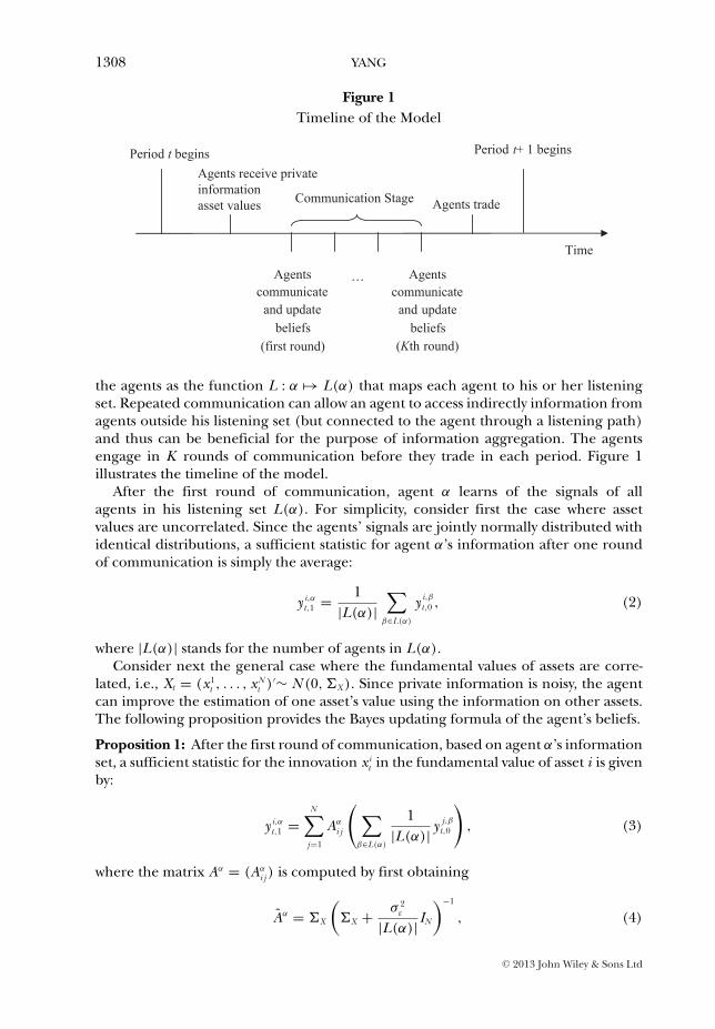
Figure 1Timeline of the Model

Period t begins Agents receive privateinformationasset values Communication Stage

Period t+ 1 begins

Agents trade

Agents communicate

and update beliefs

(first round)

Agents communicate

and update beliefs

(Kth round)

Time

…

the agents as the function L : α �→ L(α) that maps each agent to his or her listeningset. Repeated communication can allow an agent to access indirectly information fromagents outside his listening set (but connected to the agent through a listening path)and thus can be beneficial for the purpose of information aggregation. The agentsengage in K rounds of communication before they trade in each period. Figure 1illustrates the timeline of the model.

After the first round of communication, agent α learns of the signals of allagents in his listening set L(α). For simplicity, consider first the case where assetvalues are uncorrelated. Since the agents’ signals are jointly normally distributed withidentical distributions, a sufficient statistic for agent α’s information after one roundof communication is simply the average:

y i,αt,1 = 1

|L(α)|∑

β∈L(α)

y i,βt,0 , (2)

where |L(α)| stands for the number of agents in L(α).Consider next the general case where the fundamental values of assets are corre-

lated, i.e., Xt = (x1t , . . . , xN

t )′∼ N (0, �X ). Since private information is noisy, the agentcan improve the estimation of one asset’s value using the information on other assets.The following proposition provides the Bayes updating formula of the agent’s beliefs.

Proposition 1: After the first round of communication, based on agent α’s informationset, a sufficient statistic for the innovation xi

t in the fundamental value of asset i is givenby:

y i,αt,1 =

N∑j=1

Aα

i j

(∑β∈L(α)

1|L(α)| y j,β

t,0

), (3)

where the matrix Aα = (Aαi j ) is computed by first obtaining

Aα = �X

(�X + σ 2

ε

|L(α)| IN

)−1

, (4)



where IN is the identity matrix of size N × N , and then normalizing rows of Aα so thateach row sums to 1,

Aα

i j = Aαi j∑N

k=1 Aαik

. (5)

Intuitively, updating formula (3) means that agent α first averages the signals fromall agents in his listening set on each individual asset, and then derives the sufficientstatistic as a weighted average of the averaged signals on different assets using entries ofthe updating matrix Aα as weights. The sufficient statistic y i,α

t,1 will be referred to as agentα’s belief about the innovation in asset i ’s value after the first round of communication.The matrix Aα gives the Bayesian updating weights and Aα is a normalization of Aα sothat the sum of weights for each asset is equal to one.5 If the fundamental values xi

t

are uncorrelated cross-sectionally in i , i.e., �X is diagonal, then Aα = IN is the identitymatrix, and (3) reduces to the uncorrelated updating formula (2).

In the second round of communication, agent β communicates his belief y i,βt,1 to all

agents who listen to him. Each agent α then updates his belief to y i,αt,2 based on the new

information received in this round (using the formula given below). This completesthe second round of communication. In each period t , the communication amongagents continues in this way and stops after K rounds, after which the agents tradewith each other.6

The following key assumption provides the updating formula of the agent’s beliefafter each round of communication.

Assumption 1: After the k-th round of communication, agent α updates his beliefusing the following formula:

y i,αt,k =

N∑j=1

Aα

i j

(∑β∈L(α)

1|L(α)| y j,β

t,k−1

), for 1 ≤ k ≤ K . (6)

Equation (6) means that the agents apply the same formula they use in the firstround of communication (equation (2)) to later rounds of communication. Thisassumption is made to capture the fact that each agent has only limited knowledgeabout the structure of the communication network.7 In reality, an agent is only aware ofhis immediate neighbors, i.e., people in his listening set and people who listen to him.Starting from the second round of communication, the agents learn of beliefs thatcould contain information from agents not directly connected to them. Therefore, itis beyond their capacity to formulate a Bayesian updating formula after the secondround of communication. Furthermore, in reality, when an investor receives a piece

5 Such a normalization is warranted to the extent that agents communicate their beliefs, which are sufficientstatistics of their information, rather than the posteriors. Investors can ignore priors of asset values whenthey communicate since priors are common knowledge in the model.6 The number of rounds K can be regarded as exogeneously determined by the investors. K may be viewedas the number of communication rounds with which the agents believe that they would have obtainedinformation of sufficient precision for trading purposes.7 If the network is symmetric and the asset fundamentals are uncorrelated, then the formula inAssumption 1 would provide an unbiased estimate of the true fundamental values and the resulting assetprices aggregates information correctly.


1310 YANG

of information from another investor, it may be difficult to know even the numberof rounds of communication this piece of information has experienced. Assumption1 simplifies the problem faced by the agents with limited knowledge. Equation (6)is easy to implement as it allows the investors to compute a weighted average of theinformation they receive at any point of time, using time-invariant weights that onlyrequire knowledge of their listening set.8

Next I turn to the specification of the social network among agents.

Definition 1: A listening structure is said to be symmetric of degree M1 if there exists aconstant M1 such that:

• |L(α)| = M1, for all α.

• |{β : α ∈ L(β)}| = M1, for all α.

In a symmetric listening structure of degree M1, each agent listens to M1 agentsand is also listened to by exactly M1 agents. In such a network, each agent has thesame influence on the average belief of all agents and thus information is aggregatedwithout “biases”. As the focus of this paper is on the consequences of communicationwith limited knowledge (Assumption 1), rather than on the structure of the socialnetwork, I make the following assumption on the listening structure. More generalstructures of the communication network will be discussed in Section 5.(ii).

Assumption 2: The listening structure among agents is symmetric of degree M1.

In rational expectations equilibria, agents observe prices and make inferences basedon them. As we will show later, the equilibrium prices aggregate the investors’ beliefsin a certain way. Therefore, in order to define expectations and optimal portfoliochoices, we need to make assumptions about agents’ beliefs about the average beliefof all agents. Denote the average belief of investors for asset i after k rounds ofcommunication by

y it,k = 1

M

M∑α=1

y i,αt,k . (7)

I make the following assumption about agent α’s belief about the average belief ofinvestors after communication.

Assumption 3: Under agent α’s belief and information set after K rounds ofcommunication in period t , the average belief y i

t,K is a sufficient statistic of thefundamental value xi

t and

y it,K = xi

t + εit,K ,

where εit,K ∼ N (0,

σ2ε

M) is i.i.d. for 1 ≤ i ≤ N and independent of xi

t .

8 In general, even if the agents are aware of the structure of the entire communication network, theBayesian updating formulas can quickly become very complicated as the number of rounds increases. ThusAssumption 1 can also be understood as a simplified formula that allows agents with limited processingpower to update the information they receive.



This assumption means that the agents believe the average belief of all investorsafter K rounds of communication correctly aggregate information from all investors.The agents’ beliefs in this assumption are correct if the social network is symmetricand the asset fundamentals are uncorrelated.

(ii) Equilibrium

Let θαt = (θ 1,α

t , . . . , θN ,αt )′ be agent α’s positions in the risky assets after trading in period

t . I define the equilibrium of the model in the spirit of the sequential equilibrium asin Kreps and Wilson (1982).

Definition 2: An equilibrium of the model is defined to be a set of prices {Pt}1≤t≤T−1

and a collection of portfolio choices {θαt }1≤α≤N ,1≤t≤T−1 of agents such that :

1) Portfolio choices of each agent optimizes expected utility,

(θα∗t , . . . , θα∗

T−1) =arg max

(θαt ,...,θα

T−1)E α

t

[− exp

(−γ

(T−1∑s=t

θα′s (Ps+1 − Ps )

))], for 1 ≤ t ≤ T − 1.

(8)Here E α

t [ · ] = E α[ · | I αt , Pt] denotes the expectation under agent α’s belief, condi-

tional on the information set I αt after the communication stage and the price Pt in

period t .2) The financial markets clear, i.e.,

M∑α=1

θα

t = MS, 1 ≤ α ≤ N , 1 ≤ t ≤ T − 1, (9)

where S = (S1, . . . , SN )′ is the vector of (constant) per capita supply of assets.

Note that the agents learn from the equilibrium prices when making optimalportfolio choices, thus the equilibrium is similar to the standard rational expectationsequilibrium as in Radner (1979).

The following theorem proves the existence of an equilibrium and characterizesthe equilibrium prices of the model.

Theorem 2: There exists an equilibrium in which the price vectors {Pt}1≤t≤T−1 are givenby

Pt =t∑

s=1

AYs,K − (T − t − 1)γ A�X S − (T − 1)γσ 2

ε

MAS, for 1 ≤ t ≤ T − 1, (10)

where A = �X (�X + σ2ε

M)−1, Ys,K = ( y 1

s,K , . . . , y Ns,K )′ is the average belief vector of all

agents after the communication stage in period s , and S is the per capita supply vector.

The first term in equation (10) is the expectation of fundamentals based on theaverage belief of investors (the matrix A is the projection matrix of the vector offundamental values Xs on the average belief vector Ys,K , as in linear regressions). Thesecond term is the compensation for risk in Xs for s > t , and the third term is the


1312 YANG

compensation for residual risk due to the non-fully-revealing nature of prices (theprice in period t only reveals Yt,K , but not Xt).

In the equilibrium, the individual investors form their portfolios with informationfrom market price. As a result, the resulting portfolio for each investor is the same.This fact is reminiscent of the “no trade” theorem Milgrom and Stokey (1982) whereagents do not trade in rational equilibrium but the prices still reflect their information.Note also that our model is not a model with heterogeneous beliefs but rather a modelwith heterogeneous information (and limited knowledge about the social network),hence the information from prices is sufficient to ensure that all individuals hold thesame portfolio. Nevertheless, the agents’ limited knowledge about the social networkprevents information from aggregating in an unbiased way.

As in classical rational expectations equilibria, we do not model the price formationprocess. It is possible to extend the model to allow for noise traders (as in, forexample, Grossman and Stiglitz, 1980), which would provide an explicit process ofprice formation through trades. We leave this possibility for future research.

Denote the change in prices for asset i from period t − 1 to t by Rit , that is,

Rit = P i

t − P it−1. (11)

We will refer to the changes in asset prices as asset returns throughout this paper.9 LetRt = (R1

t , . . . RNt )′ be the vector of returns of risky assets. By Theorem 2, asset returns

in the equilibrium are given by

Rt = AYt,K + γ A�X S, for 2 ≤ t ≤ T − 1. (12)

3. RETURN COMOVEMENT AND FACTOR STRUCTURES

As discussed in the introduction, there is excess comovement in asset returns beyondthose in fundamental values of assets. Furthermore, a typical feature of the comove-ment of asset returns is that the first few principal components explain almost all ofthe variations in asset returns. In other words, there is a factor structure in returns.In the following, I will establish the connection between the asset return comovementand the covariance of investors’ beliefs and use this connection to explain the abovestylized facts about asset returns.

Using equation (12), the covariance of asset returns in the model is given by

Cov(Rt , Rt) = Cov(AYt,K , AYt,K ) = ACov(Yt,K , Yt,K )A. (13)

When the number of agents M is large, the matrix A = �X (�X + σ2ε

MIN )−1 is close to the

identity matrix. Studying the covariance of asset returns is thus essentially equivalentto studying the covariance of beliefs of investors after communication.

9 As prices can be negative in the model, the usual concept of return is not always well defined. It isstandard practice, however, to regard changes in asset prices as an approximation of asset returns in modelswhere asset values and prices are normally distributed.



As the listening structure is symmetric with degree M1, we can rewrite the updatingformula (6) as:

y i,αt,k =

N∑j=1

A1,i j

(∑β∈L(α)

1M1

y j,βt,k−1

), for all i, α, (14)

where A1 is obtained by normalizing A1 = �X (�X + σ2ε

M1IN ) so that each row sums to 1.

Summing both sides of (14) with respect to α, and using the fact that the listeningstructure is symmetric, we obtain the following simple updating formula for theaverage beliefs of investors after k communication rounds,

y it,k =

N∑j=1

A1,i j yj

t,k . (15)

Rewritten in vector form,

Yt,k = A1Yt,k−1. (16)

Iterated application of 16 yields

Yt,k = Ak1Yt,0. (17)

Plugging equation (17) into (13), one obtains the following representation of thecovariance matrix of returns,

Cov(Rt) = ACov(AK1 Yt,0)A = AAK

1

(�X + σ 2

ε

MIN

)AK

1 A. (18)

Studying the covariance of returns is thus equivalent to studying the matrix on theright hand side of equation (18). The eigenvalues and principal components of thismatrix are much easier to analyze if the symmetric matrices A1 and �X commute, thatis, A1�X = �X A1. The following assumption on the covariance matrix of the changesin asset fundamentals is a sufficient condition that A1 and �X commute.

Assumption 4: 1) The covariance matrix �X has distinct eigenvalues. 2) The vector1 = (1, 1, . . . , 1)′ is the eigenvector of �X with the largest eigenvalue.

The assumption that �X has distinct eigenvalues is a generic assumption, that is,the assumption is true except for a zero measure set of symmetric matrices, becausethe subset of symmetric matrices for which at least two eigenvalues are equal is alower-dimensional subset of the set of all symmetric matrices. The second part ofthe assumption states that the market factor is the first principal component of thechanges in asset fundamentals. This is consistent with the empirical evidence that thereis a strong market factor among unexpected changes in earnings (Fama and French,1995.)10 The following lemma is useful for our main results later.

10 In the real stock market, an approximate market factor, rather than the precise market factor, would bethe first principal component of changes in fundamentals. This will not change our results materially as aslight perturbation of our model still applies.


1314 YANG

Lemma 1: If Assumption 4 is true, then the matrices A1 and �X commute, i.e., A1�X =�X A1.

Let ρi be the i -th largest eigenvalue of �X , then ρi is the eigenvalue of the i -thprincipal component for X . The following theorem characterizes the eigenvalues ofthe covariance matrix of returns after communication.

Theorem 3: The i -th largest eigenvalue of the covariance matrix of returns in periodt (1 ≤ t ≤ T − 1) is given by:

ρi,K =⎛⎝ρ1 + σ2

ε

M1

ρ1· ρi

ρi + σ2ε

M1

⎞⎠2K

ρ2i

ρi + σ2ε

M

. (19)

For any i < j , as the the number of communication rounds K goes to infinity,

limK→∞

ρi,K

ρ j,K= ∞. (20)

Equation (19) relates the eigenvalues of the covariance matrix of returns to thoseof the covariance matrix of fundamental values. Intuitively, equation (20) means thatthe relative difference between the importance of any two principal componentsincreases unboundedly as the number of communication rounds increases. Witha sufficient number of communication rounds, the covariance matrix of returnsbecomes very concentrated in the sense that the relative differences between twoadjacent eigenvalues are arbitrarily large. Therefore, the covariance of asset returnsis mostly explained by the first few principal components or factors, consistent withempirical evidence found in many asset markets.

I define excess comovement in the model as follows.

Definition 3: The asset returns are said to have excess comovement if for any 1 ≤ i <

j ≤ N , the ratio of eigenvalues of the covariance matrix of returns ρi,K

ρ j,Kis greater than

the corresponding ratio of eigenvalues of the covariance matrix of fundamental valuesρiρ j

.

This definition captures the main intuition of excess comovement, that is, the firstfew principal factors in returns explain more covariance than that explained by factorsin the covariance of fundamental values. The following corollary follows easily fromTheorem 3.

Corollary 4: There is excess comovement in asset returns. The covariance matrixof returns becomes more concentrated as the number of communication roundsincreases. The extent of excess comovement and concentration of factor structure ispositively correlated with σε, the standard deviation of the noise term of agents’ signals,and K , the number of communication rounds, and negatively correlated with M1, thenumber of agents in any listening set, and M , the total number of agents.

This corollary has interesting empirical implications. For example, the more noisyinvestors’ signals are, or the fewer information sources investors have, or the lowerthe number of market participants, the more excess comovement there is in returns.These are consistent with the evidence in Morck et al. (2000), that there is more



excess comovement in stock prices in less developed countries than more developedcountries, and the evidence in Campbell et al. (2001), that there has been more excesscomovement in stock prices in the past than in the present.

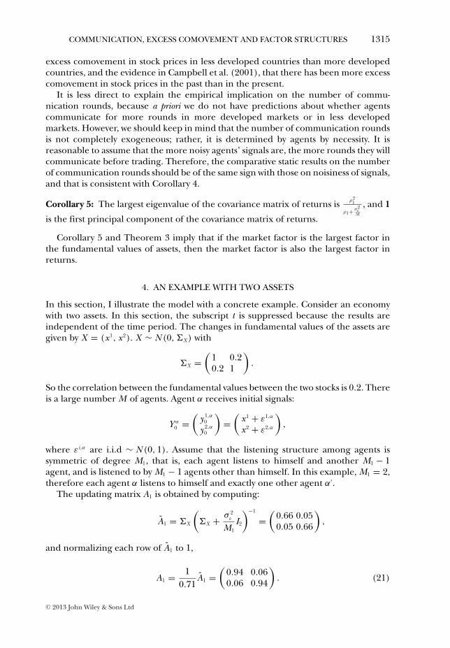
It is less direct to explain the empirical implication on the number of commu-nication rounds, because a priori we do not have predictions about whether agentscommunicate for more rounds in more developed markets or in less developedmarkets. However, we should keep in mind that the number of communication roundsis not completely exogeneous; rather, it is determined by agents by necessity. It isreasonable to assume that the more noisy agents’ signals are, the more rounds they willcommunicate before trading. Therefore, the comparative static results on the numberof communication rounds should be of the same sign with those on noisiness of signals,and that is consistent with Corollary 4.

Corollary 5: The largest eigenvalue of the covariance matrix of returns is ρ21

ρ1+ σ2ε

M

, and 1

is the first principal component of the covariance matrix of returns.

Corollary 5 and Theorem 3 imply that if the market factor is the largest factor inthe fundamental values of assets, then the market factor is also the largest factor inreturns.

4. AN EXAMPLE WITH TWO ASSETS

In this section, I illustrate the model with a concrete example. Consider an economywith two assets. In this section, the subscript t is suppressed because the results areindependent of the time period. The changes in fundamental values of the assets aregiven by X = (x1, x2). X ∼ N (0, �X ) with

�X =(

1 0.20.2 1

).

So the correlation between the fundamental values between the two stocks is 0.2. Thereis a large number M of agents. Agent α receives initial signals:

Y α

0 =(

y 1,α

0

y 2,α

0

)=(

x1 + ε1,α

x2 + ε2,α

),

where εi,α are i.i.d ∼ N (0, 1). Assume that the listening structure among agents issymmetric of degree M1, that is, each agent listens to himself and another M1 − 1agent, and is listened to by M1 − 1 agents other than himself. In this example, M1 = 2,therefore each agent α listens to himself and exactly one other agent α′.

The updating matrix A1 is obtained by computing:

A1 = �X

(�X + σ 2

ε

M1I2

)−1

=(

0.66 0.050.05 0.66

),

and normalizing each row of A1 to 1,

A1 = 10.71

A1 =(

0.94 0.060.06 0.94

). (21)


1316 YANG

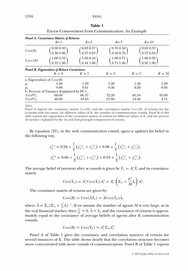
Table 1Excess Comovement from Communication: An Example

Panel A. Covariance Matrix of ReturnsK=1 K=2 K=5 K=10

Cov(R)(

0.900.30

0.300.90

) (0.830.37

0.370.83

) (0.700.50

0.500.70

) (0.630.57

0.570.63

)

Cor r (R)(

1.000.33

0.331.00

) (1.000.44

0.441.00

) (1.000.71

0.711.00

) (1.000.92

0.921.00

)Panel B. Eigenvalues of Return Covariance

K = 0 K = 1 K = 2 K = 5 K = 10

a. Eigenvalues of Cov(R)ρ1 1.20 1.20 1.20 1.20 1.20ρ2 0.80 0.61 0.46 0.20 0.05b. Percent of Variance Explained by PC’sVar PC1 60.00 66.37 72.20 85.54 95.89Var PC2 40.00 33.63 27.80 14.46 4.11

Notes:Panel A reports the covariance matrix Cov(R), and the correlation matrix Cor r (R) of returns for theeconomy with two assets, for different values of K , the number of communication rounds. Panel B of thistable reports the eigenvalues of the covariance matrix of returns for different values of K , and the percentof variance explained by the 1st and 2nd principal components of returns.

By equation (21), in the m-th communication round, agent α updates his belief inthe following way,

y 1,α

m = 0.94 × 12

(y 1,α

m−1 + y 1,α′m−1

)+ 0.06 × 12

(y 2,α

m−1 + y 2,α′m−1

),

y 2,α

m = 0.06 × 12

(y 1,α

m−1 + y 1,α′m−1

)+ 0.94 × 12

(y 2,α

m−1 + y 2,α′m−1

).

The average belief of investors after m rounds is given by Ym = Am1 Y0 and its covariance

matrix

Cov(Ym) = Am1 Cov(Y0)Am

1 = Am1

(�X + σ 2

ε

MI2

)Am

1 .

The covariance matrix of returns are given by:

Cov(R) = Cov(AYK ) = ACov(YK )A,


MI2)−1. If we assume the number of agents M is very large, as in

the real financial market, then σ2ε

M≈ 0, A ≈ I2, and the covariance of returns is approx-

imately equal to the covariance of average beliefs of agents after K communicationrounds,

Cov(R) ≈ Cov(YK ) ≈ AK1 �X AK

1 .

Panel A of Table 1 gives the covariance and correlation matrices of returns forseveral instances of K . The table shows clearly that the correlation structure becomesmore concentrated with more rounds of communications. Panel B of Table 1 reports



the eigenvalues for the principal components(PCs) of returns and the percent ofvariance explained by each PC. The gaps between the eigenvalues widen with eachround of updating. After 10 rounds of updating, the first PC, which is the marketfactor here, already explains over 95% of the variation of returns and the asset returnsexhibit a very concentrated factor structure.

5. EXTENSIONS AND APPLICATIONS

(i) Sophisticated Agents

In the basic model, all investors exhibit the same behavioral pattern when they updatebeliefs. In reality, some investors could have more knowledge about the structure of thesocial network than other investors. In this section, I consider a model with two classesof agents: naive and sophisticated. Naive agents behave the same way as the agentsin the basic model. Sophisticated agents have some knowledge about the networkstructure and exploit this knowledge in trading. Specifically, a sophisticated agent onlyuses the updating matrix A1 in the first round of communication, and simply averagessignals from agents in his listening set in later communication rounds.11

The main result is that the concentration of correlation of asset returns, still exists,but is attenuated when there are sophisticated agents. Formally, assume there is afraction μ of naive agents, who follow the updating rule (6), and 1 − μ of sophisticatedagents, who follow (6) in the first round (k = 1), and use the following updatingformula in the k-th round (k > 1),

y i,αt,k =

N∑j=1

(M∑

β=1

1|L(α)| y j,β

t,k−1

), for all i. (22)

In addition, assume that the listening structure is also symmetric with respect to thetwo types of agents in the following sense,

|{β : β ∈ L(α) and β is naive}||{β : β ∈ L(α)}| = μ, for all α.

In other words, each agent α’s listening set contains a fraction of naive agents as in theoverall population. Summing the updating equations (6) and (22) across all agents,we have:

Yt,1 = A1Yt,0, (23)

Yt,k = (μA1 + (1 − μ)IN )Yt,k−1, for k > 1. (24)

From this one can derive similar results as in Theorem 3. One can also easily showthat when there are more sophisticated agents in the economy, then there will beless excess comovement of asset prices. The intuition is that the updating matrix

11 If all agents are sophisticated and the social network is symmetric, then the aggregate belief of all agentsprovides an unbiased estimate of the fundamental values and asset prices correctly aggregate information.However, if all agents are naive, then we know from the previous sections that asset prices are biased.


1318 YANG

μA1 + (1 − μ)IN leads to less comovement than the matrix A1 in the case where allagents are naive. Morck et al. (2000) find that there is more excess comovement inthe stock markets in poor countries than in rich countries. This is consistent withour model as people in more developed countries and more mature markets aremore sophisticated than those in less developed countries and less mature markets.This result is also consistent with the time-series evidence that US stock returns arebecoming less correlated in the long-run, shown in Campbell et al. (2001), as investorsin the modern era become more sophisticated than market participants in the past.

(ii) General Listening Structures

The listening structure among agents in the basic model is assumed to be symmetric.This assumption ignores the possibility that more knowledgeable or more authoritativepeople tend to be listened to by a greater number of people. However, there canbe different hierarchies of agents in the market, and we may regard agents in thesame hierarchy as having a roughly symmetric listening structure. Agents in a lowerhierarchy listen more intensively to those in a higher hierarchy. In fact, stock prices arelargely determined by the opinions of people in the highest hierarchies, such as stockanalysts, fund managers, or economists. If agents in each hierarchy behave similarly tothe basic model, similar results on the excess comovement of asset returns to those inthe basic model then hold.

Another generalization is the possibility that agents only communicate withingroups divided by their location or other characteristics, and the agents in a particulargroup mostly communicate about the assets for which they have better information,such as stocks that are traded in their local markets. The segmentation of communica-tion among agents can be used to explain the segmentation of markets and the “homebias” of investors. For example the fact that the price of each of a pair of twin stockscomoves more with the stock prices in the local stock market, as documented in Frootand Dabora (1999).

(iii) Feedback Effects

In the basic model it is assumed that investors know the true distribution of fundamen-tal values of assets. However, if the fundamental values are not observable, investorsmay use the covariance of observed stock returns as a proxy for the covariance offundamental stock values. Because stock returns are shown in the basic model topossess excess comovement relative to fundamental values, the above practice willgenerate a feedback effect and will further increase the excess comovement of stockreturns. Therefore, the realized excess comovement of asset returns can be moresevere than those predicted in the basic model.

In fact, in such a model, if investors update their beliefs on the covariance matrixdynamically, then covariance of stock returns will finally concentrate to such an extentthat the market factor is the only determining factor of stock returns; in other words,a one-factor model fits asset returns perfectly. In reality, there are certain forces thatprevent the ever-intensifying concentration depicted above, e.g., partial observabilityof the fundamental values. As a result, we do not observe a single market factorexplaining the entire covariance structure.



6. CONCLUSION

In this paper, I develop a general equilibrium model in which investors communicatein a social network before trading. Investors repeatedly communicate in the networkbut their knowledge of the social network is limited to that of their neighbors.Therefore, investors do not fully realize the consequences of their communicationand belief updating. As a result, asset returns contain excess comovement and moreconcentrated factor structures compared to fundamental values. The model generatesseveral testable empirical predictions that are consistent with the empirical literatureon excess return comovement.

There are potential research directions that extend the current model. For exam-ple, factors may arise not only from fundamental values, but also from other investorbehaviors (e.g., Barberis and Shleifer, 2003). The model may be extended to the casewhere both fundamental factors and behavioral factors exist and they can all leadexcess comovement through the communication channel modeled here. Anotherpossible extension is to consider more general listening structures such as relativelyisolated communication networks in order to explain phenomena such as “home bias”or slow diffusion of information across different investor groups.

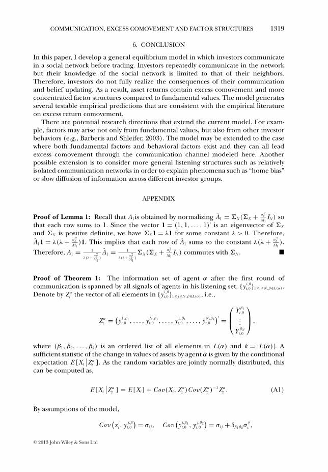
APPENDIX

Proof of Lemma 1: Recall that A1is obtained by normalizing A1 = �X (�X + σ2ε

M1IN ) so

that each row sums to 1. Since the vector 1 = (1, 1, . . . , 1)′ is an eigenvector of �X

and �X is positive definite, we have �X 1 = λ1 for some constant λ > 0. Therefore,A11 = λ(λ + σ2

ε

M1)1. This implies that each row of A1 sums to the constant λ(λ + σ2

ε

M1).

Therefore, A1 = 1

λ(λ+ σ2ε

M1)A1 = 1

λ(λ+ σ2ε

M1)�X (�X + σ2

ε

M1IN ) commutes with �N . �

Proof of Theorem 1: The information set of agent α after the first round ofcommunication is spanned by all signals of agents in his listening set, {y i,β

t,0 }1≤i≤N ,β∈L(α).Denote by Z α

t the vector of all elements in {y i,βt,0 }1≤ j≤N ,β∈L(α), i.e.,

Z α

t = (y 1,β1

t,0 , . . . , y N ,β1t,0 , . . . , y 1,βk

t,0 , . . . , y N ,βkt,0

)′ =

⎛⎜⎝

Y β1t,0...

Y βNt,0

⎞⎟⎠ ,

where (β1, β2, . . . , βk) is an ordered list of all elements in L(α) and k = |L(α)|. Asufficient statistic of the change in values of assets by agent α is given by the conditionalexpectation E [Xt

∣∣Z αt ]. As the random variables are jointly normally distributed, this

can be computed as,

E [Xt

∣∣Z α

t ] = E [Xt] + Cov(Xt , Z α

t )Cov(Z α

t )−1Z α

t . (A1)

By assumptions of the model,

Cov(xi

t , y j,βt,0

) = σi j , Cov(y i,β1

t,0 , y j,β2t,0

) = σi j + δβ1β2σ2ε,


1320 YANG

where σi j is the i j -th element of �X and δβ1β2 = 1 if β1 = β2, and = 0 otherwise. Itfollows that:

Cov(Xt , Z α

t ) = (�X , �X , . . . , �X︸︷︷︸k

) (A2)

Cov(Z α

t ) =

⎛⎜⎜⎜⎝

�X + σ 2εIN �X · · · �X

�X �X + σ 2εIN · · · �X

......

. . ....

�X �X · · · �X + σ 2εIN

⎞⎟⎟⎟⎠

︸︷︷︸k×k

(A3)

It is easy to verify using (A3) that

Cov(Z α

t )−1 = σ−2ε

⎛⎜⎜⎜⎝

− 1kAα + IN − 1

kAα · · · − 1

kAα

− 1kAα − 1

kAα + IN · · · − 1

kAα

......

. . ....

− 1kAα − 1

kAα · · · − 1

kAα + IN

⎞⎟⎟⎟⎠ , (A4)

where Aα = �X (�X + σ2ε

kIN )−1.

Now it follows from (A1), (A2), (A4), E [Xt] = 0 and �X A = �X − σ2ε

kA that

E [Xt

∣∣Z α

t ] = 1k

(k Aα, Aα, . . . , Aα︸︷︷︸)Z α

t = 1k

∑β∈L(α)

AαY β

t,0

=M∑

β=1

AαTαβY β

t,0. (A5)

Define the matrix Aα by normalizing rows of Aα so that each row sums to 1,

Aα

i j = Aαi j∑N

l=1 Aαil

. (A6)

From (A5),∑N

j=1 Aαi j (∑M

β=1 Tαβ y β

j,0) is a sufficient statistic for xit based on agent α’s

information after one round of communication. As (Aαi1, . . . , Aα

iN ) is a multiple of(Aα

i1, . . . , AαiN ), it follows that

∑Nj=1 Aα

i j

(∑Mβ=1 Tα,β y β

j,0

)is also a sufficient statistic for xi

t ,and the theorem is proved. �Proof of Theorem 2: I will show that the following prices and portfolio choices givean equilibrium,

Pt =t∑

s=1

AYs,K − (T − t − 1)γ A�X S − (T − 1)γσ 2

ε

MAS, for 1 ≤ t ≤ T − 1, (A7)

θα

t = S, for 1 ≤ t ≤ T − 1. (A8)



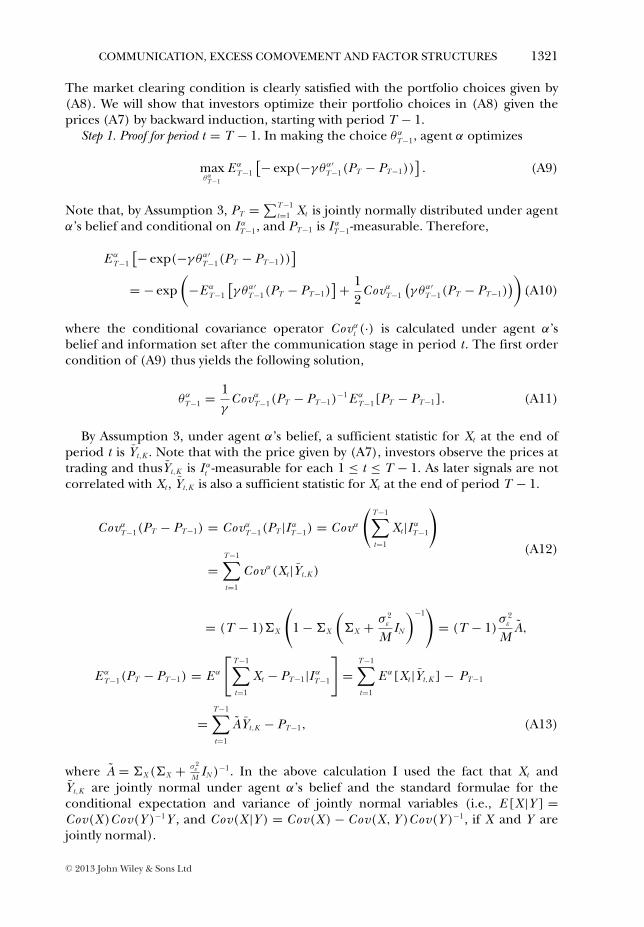
The market clearing condition is clearly satisfied with the portfolio choices given by(A8). We will show that investors optimize their portfolio choices in (A8) given theprices (A7) by backward induction, starting with period T − 1.

Step 1. Proof for period t = T − 1. In making the choice θαT−1, agent α optimizes

maxθα

T−1

E α

T−1

[− exp(−γ θα′T−1(PT − PT−1))

]. (A9)

Note that, by Assumption 3, PT = ∑T−1t=1 Xt is jointly normally distributed under agent

α’s belief and conditional on I αT−1, and PT−1 is I α

T−1-measurable. Therefore,

E α

T−1

[− exp(−γ θα′T−1(PT − PT−1))

]= − exp

(−E α

T−1

[γ θα′

T−1(PT − PT−1)]+ 1

2Covα

T−1

(γ θα′

T−1(PT − PT−1)))

.(A10)

where the conditional covariance operator Covαt (·) is calculated under agent α’s

belief and information set after the communication stage in period t . The first ordercondition of (A9) thus yields the following solution,

θα

T−1 = 1γ

Covα

T−1(PT − PT−1)−1 E α

T−1[PT − PT−1]. (A11)

By Assumption 3, under agent α’s belief, a sufficient statistic for Xt at the end ofperiod t is Yt,K . Note that with the price given by (A7), investors observe the prices attrading and thusYt,K is I α

t -measurable for each 1 ≤ t ≤ T − 1. As later signals are notcorrelated with Xt , Yt,K is also a sufficient statistic for Xt at the end of period T − 1.

CovαT−1(PT − PT−1) = Covα

T−1(PT |I αT−1) = Covα

(T−1∑t=1

Xt |I α

T−1

)

=T−1∑t=1

Covα(Xt |Yt,K )

(A12)

= (T − 1)�X

(1 − �X

(�X + σ 2

ε

MIN

)−1)

= (T − 1)σ 2

ε

MA,

E α

T−1(PT − PT−1) = E α

[T−1∑t=1

Xt − PT−1|I α

T−1

]=

T−1∑t=1

E α[Xt |Yt,K ] − PT−1

=T−1∑t=1

AYt,K − PT−1, (A13)


MIN )−1. In the above calculation I used the fact that Xt and

Yt,K are jointly normal under agent α’s belief and the standard formulae for theconditional expectation and variance of jointly normal variables (i.e., E [X |Y ] =Cov(X )Cov(Y )−1Y , and Cov(X |Y ) = Cov(X ) − Cov(X, Y )Cov(Y )−1, if X and Y arejointly normal).


1322 YANG

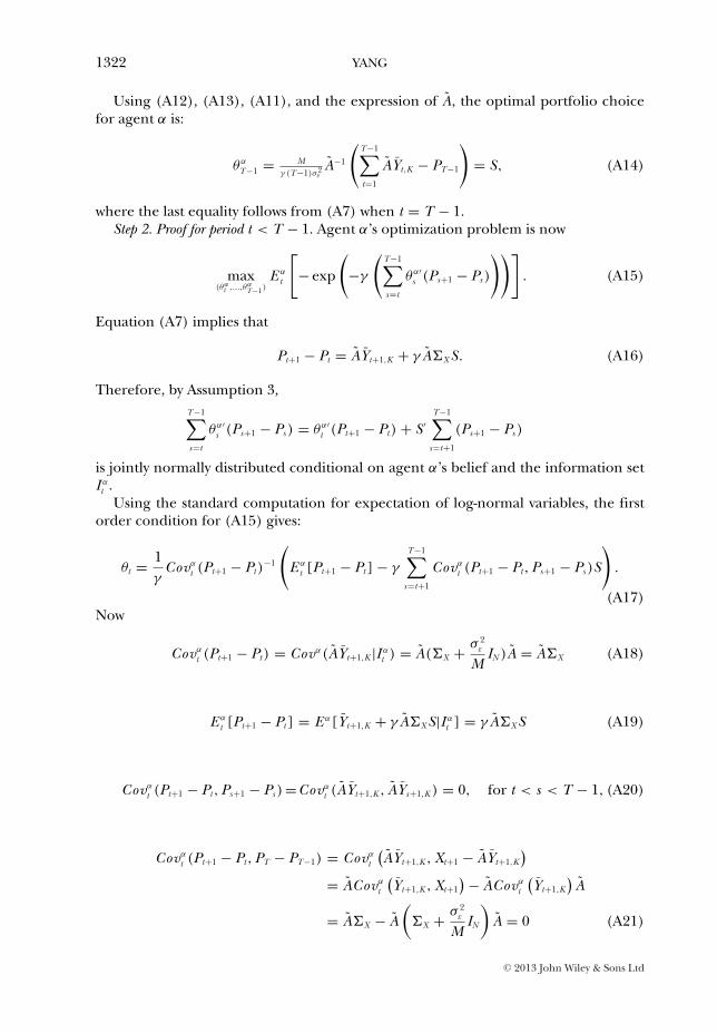
Using (A12), (A13), (A11), and the expression of A, the optimal portfolio choicefor agent α is:

θα

T−1 = Mγ (T−1)σ2

εA−1

(T−1∑t=1

AYt,K − PT−1

)= S, (A14)

where the last equality follows from (A7) when t = T − 1.Step 2. Proof for period t < T − 1. Agent α’s optimization problem is now

max(θα

t ,...,θαT−1)

E α

t

[− exp

(−γ

(T−1∑s=t

θα′s (Ps+1 − Ps )

))]. (A15)

Equation (A7) implies that

Pt+1 − Pt = AYt+1,K + γ A�X S. (A16)

Therefore, by Assumption 3,T−1∑s=t

θα′s (Ps+1 − Ps ) = θα′

t (Pt+1 − Pt) + S ′T−1∑

s=t+1

(Ps+1 − Ps )

is jointly normally distributed conditional on agent α’s belief and the information setI α

t .Using the standard computation for expectation of log-normal variables, the first

order condition for (A15) gives:

θt = 1γ

Covα

t (Pt+1 − Pt)−1

(E α

t [Pt+1 − Pt] − γ

T−1∑s=t+1

Covα

t (Pt+1 − Pt , Ps+1 − Ps )S

).

(A17)Now

Covα

t (Pt+1 − Pt) = Covα(AYt+1,K |I αt ) = A(�X + σ 2

ε

MIN )A = A�X (A18)

E α

t [Pt+1 − Pt] = E α[Yt+1,K + γ A�X S|I αt ] = γ A�X S (A19)

Covα

t (Pt+1 − Pt , Ps+1 − Ps )=Covαt (AYt+1,K , AYs+1,K ) = 0, for t < s < T − 1, (A20)

Covα

t (Pt+1 − Pt , PT − PT−1) = Covα

t

(AYt+1,K , Xt+1 − AYt+1,K

)= ACovα

t

(Yt+1,K , Xt+1

)− ACovα

t

(Yt+1,K

)A

= A�X − A(

�X + σ 2ε

MIN

)A = 0 (A21)



Plugging equations (A18), (A19), (A20), and (A21) into (A17), we find that θαt = S. �

Proof of Theorem 3: Denote the i -th principal component of �X = Cov(X ) by fi =∑Nj=1 vi j X j , where vi = (vi1, . . . , viN )′ gives an orthonormal basis of RN . The matrix

U = (vi j )′ is then an orthogonal matrix, and hence U ′ = U −1. Using the vectornotation Ft = ( f 1

t , ..., f Nt )′, then Ft = U ′Xt and Xt = (U ′)−1Ft = U Ft . The covariance

matrix Cov(Ft ) = D is diagonal with diagonal entries (ρ1, . . . , ρN ). The covariancematrix �X is thus diagonalized by the matrix U ,

�X = U DU ′. (A22)

Note that �X + σ2ε

M1IN = U (D + σ2

ε

M1IN )U ′, also diagonalizable by U . This implies that

A1 = �X

(�X + σ 2

ε

M1IN

)−1

= U D(

D + σ 2ε

M1IN

)−1

U ′ = U

⎛⎜⎜⎜⎜⎜⎜⎜⎜⎝

ρ1

ρ1 + σ 2ε

M1

· · · 0

.... . .

...

0 · · · ρN

ρN + σ 2ε

M1

⎞⎟⎟⎟⎟⎟⎟⎟⎟⎠

U ′.

(A23)

Lemma 2: The sum of all the elements in each row of A1 is equal to ρ1

ρ1+ σ2ε

M1

.

Proof: The (i, j)-th element in A1 is given by∑N

l=1 vliρl

ρl + σ2ε

M1

vl j . Therefore, the sum of

all elements in the i -th row of A1 is given by:

N∑l=1

ρl

ρl + σ2ε

M1

vli

(N∑

j=1

vl j

). (A24)

By Assumption (4), v1 = 1√N

1 = 1√N

(1, 1, . . . , 1). Since v1 and vl are orthogonal forl > 1,

N∑j=1

vl j = 0, for l > 1. (A25)

Equations (A24) and (A25) imply that the sum of each row of A1 is equal to ρ1

ρ1+ σ2ε

M1

. �

Lemma 2 implies that the updating matrix A1 is given by:

A1 =ρ1 + σ 2

ε

M1

ρ1A1 = U

⎛⎜⎜⎝

ρ1 + σ 2ε

M1

ρ1D(

D + σ 2ε

M1IN

)−1

⎞⎟⎟⎠U ′. (A26)


1324 YANG

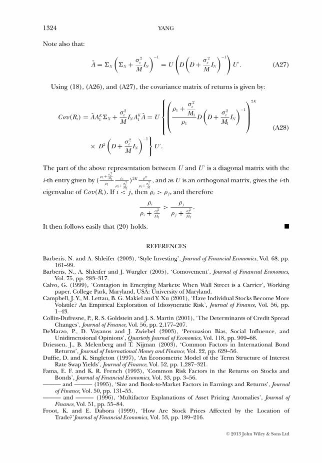
Note also that:

A = �X

(�X + σ 2

ε

MIN

)−1

= U

(D(

D + σ 2ε

MIN

)−1)

U ′. (A27)

Using (18), (A26), and (A27), the covariance matrix of returns is given by:

Cov(Rt ) = AAK1 �X + σ 2

ε

MIN AK

1 A = U

⎧⎪⎪⎪⎨⎪⎪⎪⎩

⎛⎜⎜⎝

ρ1 + σ 2ε

M1

ρ1D(

D + σ 2ε

M1IN

)−1

⎞⎟⎟⎠

2K

× D2

(D + σ 2

ε

MIN

)−1}

U ′.

(A28)

The part of the above representation between U and U ′ is a diagonal matrix with the

i -th entry given by (ρ1+ σ2

εM1

ρ1

ρi

ρi + σ2ε

M1

)2K ρ2

ρi + σ2ε

M

, and as U is an orthogonal matrix, gives the i -th

eigenvalue of Cov(Rt ). If i < j , then ρi > ρ j , and therefore

ρi

ρi + σ2ε

M1

>ρ j

ρ j + σ2ε

M1

.

It then follows easily that (20) holds. �

REFERENCES

Barberis, N. and A. Shleifer (2003), ‘Style Investing’, Journal of Financial Economics, Vol. 68, pp.161–99.

Barberis, N., A. Shleifer and J. Wurgler (2005), ‘Comovement’, Journal of Financial Economics,Vol. 75, pp. 283–317.

Calvo, G. (1999), ‘Contagion in Emerging Markets: When Wall Street is a Carrier’, Workingpaper, College Park, Maryland, USA: University of Maryland.

Campbell, J. Y., M. Lettau, B. G. Makiel and Y. Xu (2001), ‘Have Individual Stocks Become MoreVolatile? An Empirical Exploration of Idiosyncratic Risk’, Journal of Finance, Vol. 56, pp.1–43.

Collin-Dufresne, P., R. S. Goldstein and J. S. Martin (2001), ‘The Determinants of Credit SpreadChanges’, Journal of Finance, Vol. 56, pp. 2,177–207.

DeMarzo, P., D. Vayanos and J. Zwiebel (2003), ‘Persuasion Bias, Social Influence, andUnidimensional Opinions’, Quarterly Journal of Economics, Vol. 118, pp. 909–68.

Driessen, J., B. Melenberg and T. Nijman (2003), ‘Common Factors in International BondReturns’, Journal of International Money and Finance, Vol. 22, pp. 629–56.

Duffie, D. and K. Singleton (1997), ‘An Econometric Model of the Term Structure of InterestRate Swap Yields’, Journal of Finance, Vol. 52, pp. 1,287–321.

Fama, E. F. and K. R. French (1993), ‘Common Risk Factors in the Returns on Stocks andBonds’, Journal of Financial Economics, Vol. 33, pp. 3–56.

——— and ——— (1995), ‘Size and Book-to-Market Factors in Earnings and Returns’, Journalof Finance, Vol. 50, pp. 131–55.

——— and ——— (1996), ‘Multifactor Explanations of Asset Pricing Anomalies’, Journal ofFinance, Vol. 51, pp. 55–84.

Froot, K. and E. Dabora (1999), ‘How Are Stock Prices Affected by the Location ofTrade?’Journal of Financial Economics, Vol. 53, pp. 189–216.



Greenwood, R. (2008), ‘Excess Comovement of Stock Returns: Evidence from Cross-SectionalVariation in Nikkei 225 Weights’, Review of Financial Studies, Vol. 21, pp. 1,153–86.

Greenwood, R. and N. Sosner (2007), ‘Trading Patterns and Excess Comovement of StockReturns’, Financial Analyst Journal, Vol. 63, pp. 69–81.

Grossman, S. and J. Stiglitz (1980), ‘On the Impossibility of Informationally Efficient Markets’,American Economic Review, Vol. 70, pp. 393–408.

Hong, H., J. D. Kubik and J. C. Stein (2005), ‘Thy Neighbor’s Portfolio: Word-of-Mouth Effectsin the Holdings and Trades of Money Managers’, Journal of Finance, Vol. 60, pp. 2,801–24.

Kodres, L. E. and M. Pritsker (2002), ‘A Rational Expectations Model of Financial Contagion’,Journal of Finance, Vol. 57, pp. 769–99.

Kreps, D. M. and R. Wilson (1982), ‘Sequential Equilibria’, Econometrica, Vol. 50, pp. 863–94.Kyle, A. S. and W. Xiong (2001), ‘Contagion as a Wealth Effect’, Journal of Finance, Vol. 56, pp.

1,401–40.Litterman, R. and J. Scheinkman (1991), ‘Common Factors Affecting Bond Returns’, Journal of

Fixed Income, Vol. 1, pp. 54–61.Milgrom, P. and N. Stokey (1982), ‘Information, Trade and Common Knowledge’, Journal of

Economic Theory, Vol. 26, pp. 17–27.Mok, H. M. K., K. Lam and I. Cheung (1992), ‘Family Control and Return Covariation in Hong

Kong’s Common Stocks’, Journal of Business Finance and Accounting, Vol. 19, 277–93.Morck, R., B. Yeung and W. Yu (2000), ‘The Information Content of Stock Markets: Why

Do Emerging Markets Have Synchronous Stock Price Movements?’ Journal of FinancialEconomics, Vol. 58, pp. 215–60.

Pindyck, R. S. and J. J. Rotemberg (1990), ‘The Excess Comovement of Commodity Prices’,Economic Journal, Vol. 100, pp. 1,173–89.

Pindyck, R. S. and J. J. Rotemberg (1993), ‘The Comovement of Stock Prices’, Quarterly Journalof Economics, Vol. 108, pp. 1,073–104.

Radner, R. (1979), ‘Rational Expectations Equilibrium: Generic Existence and the InformationRevealed by Prices’, Econometrica, Vol. 47, pp. 665–78.

Sabherwal, S., S. K. Sarkar and Y. Zhang (2011), ‘Do Internet Stock Message Boards InfluenceTrading? Evidence from Heavily Discussed Stocks with No Fundamental News’, Journal ofBusiness Finance and Accounting, Vol. 38, pp. 1,209–37.

Singleton, K. (1995), ‘Yield Curve Risk Management for Government Bond Portfolios: AnInternational Comparison’, in W. Beaver and G. Parker (Eds.), Risk Management Problemsand Solutions, Mc-Graw Hill, New York. pp. 295–322.

Veldkamp, L. L. (2006), ‘Information Markets and the Comovement of Asset Prices’, Review ofEconomic Studies, Vol. 73, pp. 823–45.

Vijh, A. M. (1994), ‘S&P 500 Trading Strategies and Stock Betas’, Review of Financial Studies,Vol. 7, pp. 215–51.


Documents

Communication, Excess Comovement and Factor …fncbyy/Papers/Yang_2013_JBFA.pdf · Communication, Excess Comovement and ... (Peter Pope), Vikas Agarwal, Snehal Banerjee, Peter DeMarzo,