Communication Performance in Network-on-Chipspetel71/NoC/lecture-notes/lect1part2.pdfCommunication Performance in Network-on-Chips Axel Jantsch Royal Institute of Technology, Stockholm

Communication Performance in Network-on-Chips

Axel JantschRoyal Institute of Technology, Stockholm

November 24, 2004

Network on Chip Seminar, Linkoping, November 25, 2004 Communication Performance In NoCs - 1

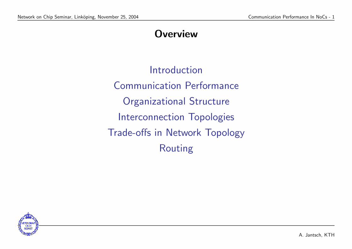
Overview

Introduction

Communication Performance

Organizational Structure

Interconnection Topologies

Trade-offs in Network Topology

Routing

A. Jantsch, KTH


IntroductionInterconnectionNetwork

Networkinterface

Communicationassistm

Mem P

Networkinterface

Communicationassistm

Mem P

• Topology: How switches andnodes are connected

• Routing algorithm: determinesthe route from source todestination

• Switching strategy: how amessage traverses the route

• Flow control: Schedules thetraversal of the message overtime

A. Jantsch, KTH


Basic Definitions

Message is the basic communication entity.Flit is the basic flow control unit. A message consists of 1 or

many flits.Phit is the basic unit of the physical layer.Direct network is a network where each switch connects to

a node.Indirect network is a network with switches not connected

to any node.Hop is the basic communication action from node to switch

or from switch to switch.Diameter is the length of the maximum shortest path

between any two nodes measured in hops.Routing distance between two nodes is the number of hops

on a route.Average distance is the average of the routing distance

over all pairs of nodes.

A. Jantsch, KTH


Basic Switching Techniques

Circuit Switching A real or virtual circuit establishes adirect connection between source and destination.

Packet Switching Each packet of a message is routedindependently. The destination address has to be providedwith each packet.

Store and Forward Packet Switching The entire packet isstored and then forwarded at each switch.

Cut Through Packet Switching The flits of a packet arepipelined through the network. The packet is notcompletely buffered in each switch.

Virtual Cut Through Packet Switching The entire packetis stored in a switch only when the header flit is blockeddue to congestion.

Wormhole Switching is cut through switching and all flitsare blocked on the spot when the header flit is blocked.

A. Jantsch, KTH

Network on Chip Seminar, Linkoping, November 25, 2004 Performance - 5

Latency

3

A

B

C

D

21 4

Time(n) = Admission + ChannelOccupancy + RoutingDelay + ContentionDelay

Admission is the time it takes to emit the message into the network.

ChannelOccupancy is the time a channel is occupied.

RoutingDelay is the delay for the route.

ContentionDelay is the delay of a message due to contention.

A. Jantsch, KTH


Channel Occupancy

ChannelOccupancy =n + nE

b

n ... message size in bitsnE ... envelop size in bitsb ... raw bandwidth of the channel

A. Jantsch, KTH


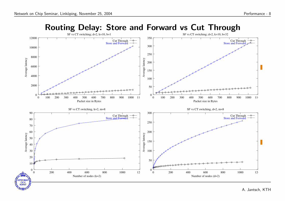
Routing Delay

Store and Forward:Tsf(n, h) = h(n

b + ∆)

Circuit Switching:Tcs(n, h) = n

b + h∆

Cut Through:Tct(n, h) = n

b + h∆

Store and Forward withfragmented packets:

Tsf(n, h, np) = n−np

b + h(np

b + ∆)

n ... message size in bitsnp ... size of message fragments in bitsh ... number of hopsb ... raw bandwidth of the channel∆ ... switching delay per hop

A. Jantsch, KTH


Routing Delay: Store and Forward vs Cut Through

0

2000

4000

6000

8000

10000

12000

0 100 200 300 400 500 600 700 800 900 1000 1100

Ave

rage

late

ncy

Packet size in Bytes

SF vs CT switching; d=2, k=10, b=1

Cut ThroughStore and Forward

0

50

100

150

200

250

300

350

0 100 200 300 400 500 600 700 800 900 1000 1100

Ave

rage

late

ncy

Packet size in Bytes

SF vs CT switching; d=2, k=10, b=32


0

10

20

30

40

50

60

70

80

90

0 200 400 600 800 1000 1200

Ave

rage

late

ncy

Number of nodes (k=2)

SF vs CT switching, k=2, m=8


0

50

100

150

200

250

300

0 200 400 600 800 1000 1200

Ave

rage

late

ncy

Number of nodes (d=2)

SF vs CT switching, d=2, m=8


A. Jantsch, KTH


Local and Global Bandwidth

Local bandwidth = b(

nn+nE+w∆

)Total bandwidth = Cb[bits/second] = Cw[bits/cycle] = C[phits/cycle]

Bisection bandwidth ... minimum bandwidth to cut the net into two equal parts.

b ... raw bandwidth of a link;

n ... message size;

nE ... size of message envelope;

w ... link bandwidth per cycle;

∆ ... switching time for each switch in cycles;

w∆ ... bandwidth lost during switching;

C ... total number of channels;

For a k×k mesh with bidirectional channels:

Total bandwidth = (4k2 − 4k)bBisection bandwidth = 2kb

3

A

B

C

D

21 4

A. Jantsch, KTH


Link and Network Utilization

total load on the network: L =Nhl

M[phits/cycle]

load per channel: ρ =Nhl

MC[phits/cycle] ≤ 1

M ... each host issues a packet every M cyclesC ... number of channelsN ... number of nodesh ... average routing distancel = n/w ... number of cycles a message occupies a channeln ... average message sizew ... bitwidth per channel

A. Jantsch, KTH


Network SaturationD

eliv

ered

ban

dwid

th

Offered bandwidth

Network saturation

Lat

ency

Delivered bandwidth

Network saturation

Typical saturation points are between 40% and 70%.The saturation point depends on

• Traffic pattern

• Stochastic variations in traffic

• Routing algorithm

A. Jantsch, KTH

Network on Chip Seminar, Linkoping, November 25, 2004 Organizational Structure - 12

Organizational Structure

• Link

• Switch

• Network Interface

A. Jantsch, KTH


Link

Short link At any time there is only one data word on thelink.

Long link Several data words can travel on the linksimultaneously.

Narrow link Data and control information is multiplexed onthe same wires.

Wide link Data and control information is transmitted inparallel and simultaneously.

Synchronous clocking Both source and destination operateon the same clock.

Asynchronous clocking The clock is encoded in thetransmitted data to allow the receiver to sample at theright time instance.

A. Jantsch, KTH


Switch

Crossbar

Control(Routing, Scheduling)

InputbufferReceiver

Outputbuffer Transmitter

Inputports

Outputports

A. Jantsch, KTH


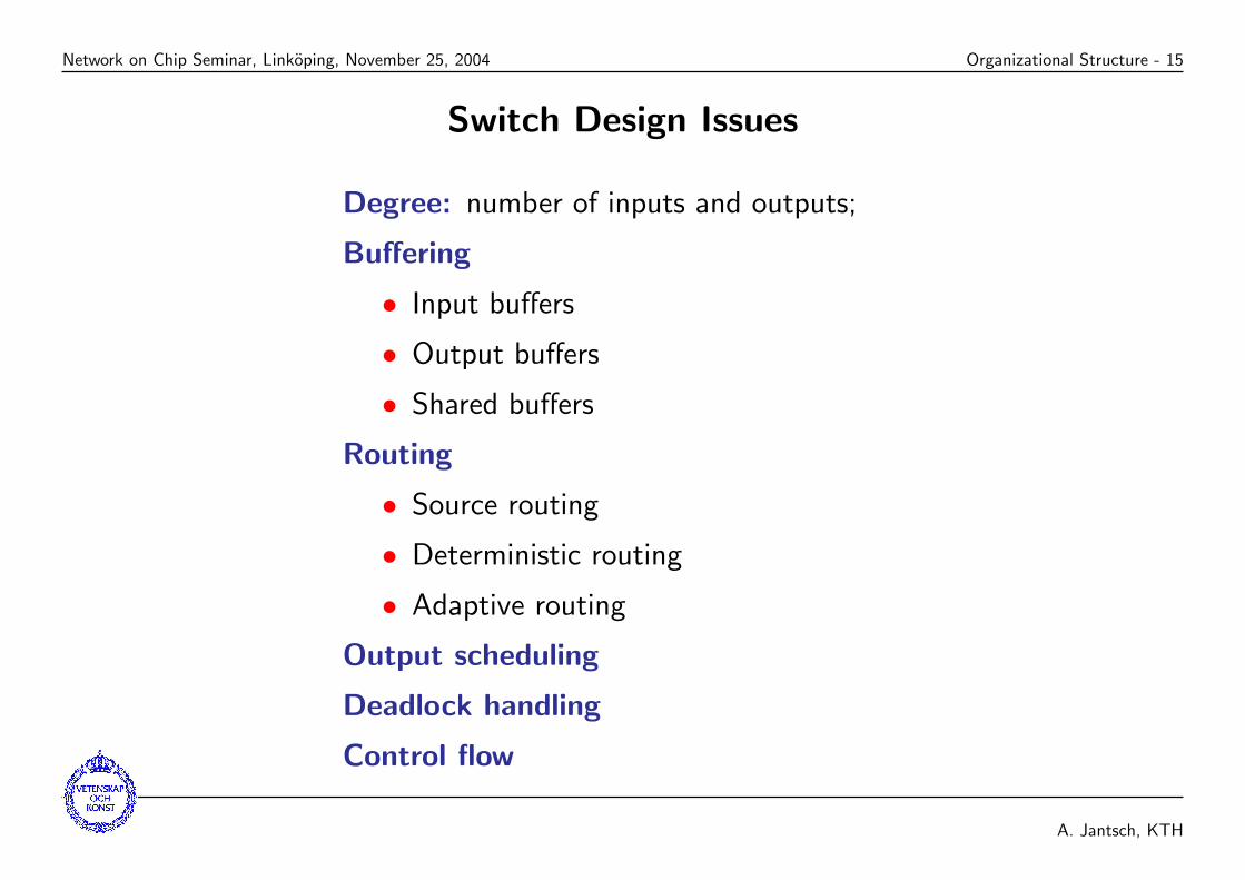
Switch Design Issues

Degree: number of inputs and outputs;

Buffering

• Input buffers

• Output buffers

• Shared buffers

Routing

• Source routing

• Deterministic routing

• Adaptive routing

Output scheduling

Deadlock handling

Control flow

A. Jantsch, KTH


Network Interface

• Admission protocol

• Reception obligations

• Buffering

• Assembling and disassemblingof messages

• Routing

• Higher level services andprotocols

A. Jantsch, KTH

Network on Chip Seminar, Linkoping, November 25, 2004 Topologies - 17

Interconnection Topologies

• Fully connected networks

• Linear arrays and rings

• Multidimensional meshes and tori

• Trees

• Butterflies

A. Jantsch, KTH


Fully Connected Networks

Node Node

Node

Node

Node

Node

Bus: switch degree = Ndiameter = 1distance = 1network cost = O(N)total bandwidth = bbisectionbandwidth

= b

Crossbar: switch degree = Ndiameter = 1distance = 1network cost = O(N2)total bandwidth = Nbbisectionbandwidth

= Nb

A. Jantsch, KTH


Linear Arrays and Rings

Torus

Linear array

Folded torus

Lineararray: switch degree = 2

diameter = N − 1distance ∼ 2/3Nnetwork cost = O(N)total bandwidth = 2(N − 1)bbisectionbandwidth

= 2b

Torus: switch degree = 2diameter = N/2distance ∼ 1/3Nnetwork cost = O(N)total bandwidth = 2Nbbisectionbandwidth

= 4b

A. Jantsch, KTH


Multidimensional Meshes and Tori

2−d torus

3−d cube

2−d mesh

k-ary d-cubes are d-dimensional tori withunidirectional links and k nodes in eachdimension:

number of nodes N = kd

switch degree = d

diameter = d(k − 1)

distance ∼ d12(k − 1)

network cost = O(N)

total bandwidth = 2Nb

bisection bandwidth = 2k(d−1)b

A. Jantsch, KTH


Routing Distance in k-ary n-Cubes

0

5

10

15

20

25

30

35

40

45

0 200 400 600 800 1000 1200

Ave

rage

dis

tanc

e

Number of nodes

Network Scalability wrt Distance

k=2d=4d=3d=2

A. Jantsch, KTH


Projecting High Dimensional Cubes

2−ary 4−cube 2−ary 5−cube

2−ary 3−cube2−ary 2−cube

A. Jantsch, KTH


Binary Trees

0

1

2

3

4 number of nodes N = 2d

number of switches = 2d − 1switch degree = 3diameter = 2ddistance ∼ d + 2network cost = O(N)total bandwidth = 2 · 2(N − 1)bbisection bandwidth = 2b

A. Jantsch, KTH


k-ary Trees

0

1

2

3

4 number of nodes N = kd

number of switches ∼ kd

switch degree = k + 1diameter = 2ddistance ∼ d + 2network cost = O(N)total bandwidth = 2 · 2(N − 1)bbisection bandwidth = kb

A. Jantsch, KTH


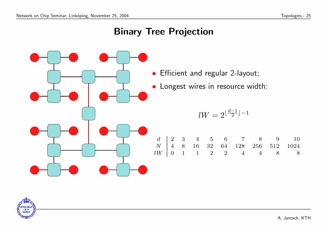
Binary Tree Projection

• Efficient and regular 2-layout;

• Longest wires in resource width:

lW = 2bd−12 c−1

d 2 3 4 5 6 7 8 9 10N 4 8 16 32 64 128 256 512 1024lW 0 1 1 2 2 4 4 8 8

A. Jantsch, KTH


k-ary n-Cubes versus k-ary Trees

k-ary n-cubes:


switch degree = d + 2



network cost = O(N)



k-ary trees:


number of switches ∼ kd

switch degree = k + 1diameter = 2d

distance ∼ d + 2network cost = O(N)total bandwidth = 2 · 2(N − 1)bbisection bandwidth = kb

A. Jantsch, KTH


Butterflies

0 1 0 1

0 10

0 10

Butterflybuildingblock

4

0

1

2

3

16 nodebutterfly

A. Jantsch, KTH


Butterfly Characteristics

4

0

1

2

3

number of nodes N = 2d

number of switches = 2d−1d

switch degree = 2diameter = d + 1distance = d + 1network cost = O(Nd)total bandwidth = 2ddb

bisection bandwidth = N2 b

A. Jantsch, KTH


k-ary n-Cubes versus k-ary Trees vs Butterflies

k-ary n-cubes binary tree butterfly

cost per node O(N) O(N) O(N log N)

distance 12

d√

N log N 2 log N log N

links per node 2 2 log N

bisection 2Nd−1

d 1 12N

frequency limit ofrandom traffic

1/( d

√N2 ) 1/N 1/2

A. Jantsch, KTH


Problems with Butterflies

• Cost of the network

? O(N log N)

? 2-d layout is more difficult than for binary trees

? Number of long wires grows faster than for trees.

• For each source-destination pair there is only one route.

• Each route blocks many other routes.

A. Jantsch, KTH


Benes Networks

• Many routes;

• Costly to computenon-blocking routes;

• High probability fornon-blocking route byrandomly selecting anintermediate node[Leighton, 1992];

A. Jantsch, KTH


Fat Trees

fat n

odes

16−node 2−ary fat−tree

A. Jantsch, KTH


k-ary n-dimensional Fat Tree Characteristicsfa

t nod

es

16−node 2−ary fat−tree


number of switches = kd−1d

switch degree = 2k

diameter = 2d

distance ∼ d

network cost = O(Nd)total bandwidth = 2kddb

bisection bandwidth = 2kd−1b

A. Jantsch, KTH


k-ary n-Cubes versus k-ary d-dimensional Fat Trees

k-ary n-cubes:


switch degree = d



network cost = O(N)



k-ary n-dimensional fat trees:


number of switches = kd−1d

switch degree = 2k

diameter = 2d

distance ∼ d

network cost = O(Nd)total bandwidth = 2kddb

bisection bandwidth = 2kd−1b

A. Jantsch, KTH


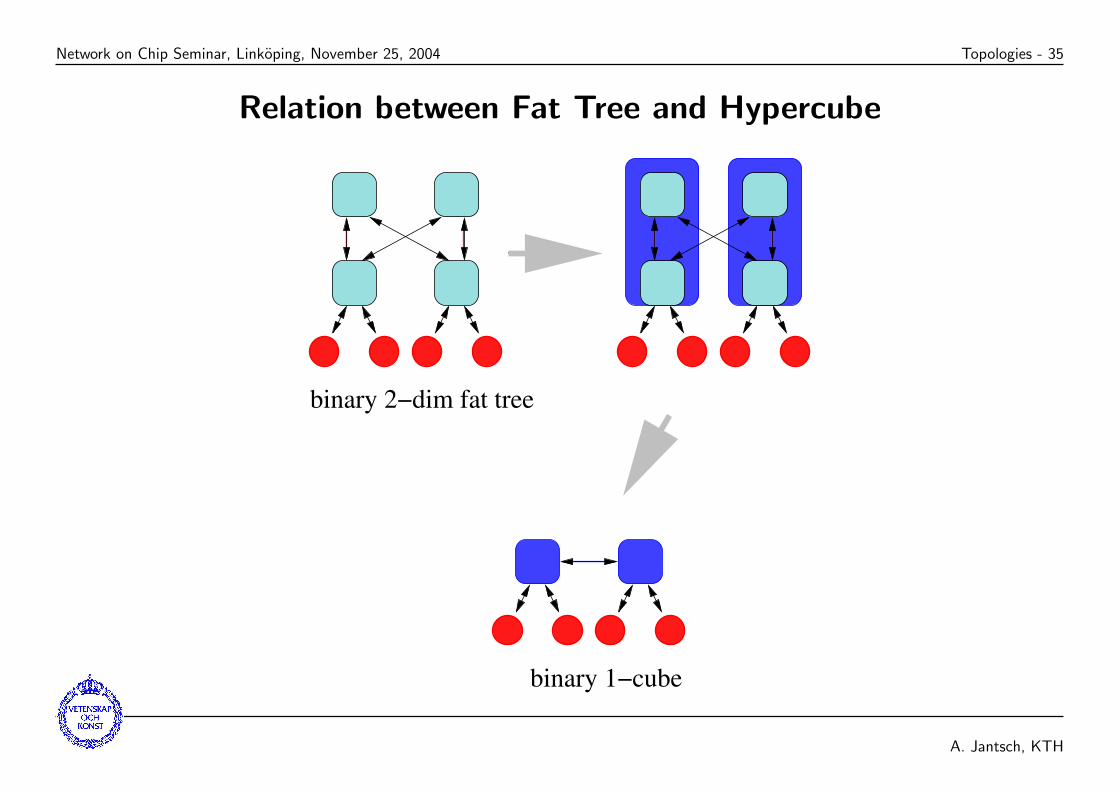
Relation between Fat Tree and Hypercube

binary 2−dim fat tree

binary 1−cube

A. Jantsch, KTH


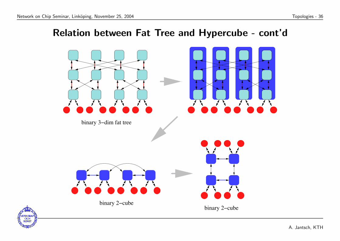
Relation between Fat Tree and Hypercube - cont’d

binary 2−cubebinary 2−cube


A. Jantsch, KTH


Relation between Fat Tree and Hypercube - cont’d

binary 3−cube


binary 3−cube

A. Jantsch, KTH


Topologies of Parallel Computers

Machine TopologyCycleTime [ns]

Channelwidth[bits]

Routingdelay[cycles]

Flit size[bits]

nCUBE/2 Hypercube 25 1 40 32TMC CM-5 Fat tree 25 4 10 4IBM SP-2 Banyan 25 8 5 16Intel Paragon 2D Mesh 11.5 16 2 16Meiko CS-2 Fat tree 20 8 7 8Cray T3D 3D Torus 6.67 16 2 16DASH Torus 30 16 2 16J-Machine 3D Mesh 31 8 2 8Monsoon Butterfly 20 16 2 16SGI Origin Hypercube 2.5 20 16 160Myricom Arbitrary 6.25 16 50 16

A. Jantsch, KTH

Network on Chip Seminar, Linkoping, November 25, 2004 Trade-offs in Topologies - 39

Trade-offs in Topology Design for the k-ary n-Cube

• Unloaded Latency

• Latency under Load

A. Jantsch, KTH


Network Scaling for Unloaded Latency

Latency(n) = Admission + ChannelOccupancy

+RoutingDelay + ContentionDelay

RoutingDelay Tct(n, h) =n

b+ h∆

RoutingDistance h =12d(k − 1) =

12(k − 1) logk N =

12(d d√

N − 1)

20

40

60

80

100

120

140

160

0 1000 2000 3000 4000 5000 6000 7000 8000 9000 10000

Ave

rage

late

ncy

Number of nodes

Network scalabilit wrt latency (m=32)

k=2d=5d=4d=3d=2

120

140

160

180

200

220

240

260

0 1000 2000 3000 4000 5000 6000 7000 8000 9000 10000

Ave

rage

late

ncy

Number of nodes


k=2d=5d=4d=3d=2

A. Jantsch, KTH


Unloaded Latency for Small Networks and Local Traffic

129

130

131

132

133

134

135

136

137

10 20 30 40 50 60 70 80 90 100

Ave

rage

late

ncy

Number of nodes


k=2d=5d=4d=3d=2

129

129.5

130

130.5

131

131.5

132

10 20 30 40 50 60 70 80 90 100

Ave

rage

late

ncy

Number of nodes

Network scalabilit wrt latency (m=128; h=dk/5)

k=2d=5d=4d=3d=2

125

130

135

140

145

150

155

160

165

170

0 1000 2000 3000 4000 5000 6000 7000 8000 9000 10000

Ave

rage

late

ncy

Number of nodes

Network scalabilit wrt latency (m=128; h=dk/5)

k=2d=5d=4d=3d=2

A. Jantsch, KTH


Unloaded Latency under a Free-Wire Cost Model

Free-wire cost model: Wires are free and can be addedwithout penalty.

0

20

40

60

80

100

120

2 3 4 5 6 7

Ave

rage

late

ncy

Dimension

Latency wrt dimension under free−wire cost model (m=32;b=32)

N=16KN=1K

N=256N=128

N=64

0

20

40

60

80

100

120

2 3 4 5 6 7A

vera

ge la

tenc

yDimension

Latency wrt dimension under free−wire cost model (m=128;b=32)

N=16KN=1K

N=256N=128

N=64

A. Jantsch, KTH


Unloaded Latency under a Fixed-Wire Cost Models

Fixed-wire cost model: The number of wires is constant pernode:128 wires per node: w(d) = b64

d c.

d 2 3 4 5 6 7 8 9 10w(d) 32 21 16 12 10 9 8 7 6

0

20

40

60

80

100

120

2 3 4 5 6 7 8 9 10

Ave

rage

late

ncy

Dimension

Latency wrt dimension under fixed−wire cost model (m=32;b=64/d)

N=16KN=1K

N=256N=128

N=64

0

20

40

60

80

100

120

2 3 4 5 6 7 8 9 10

Ave

rage

late

ncy

Dimension

Latency wrt dimension under fixed−wire cost model (m=128;b=64/d)

N=16KN=1K

N=256N=128

N=64

A. Jantsch, KTH


Unloaded Latency under a Fixed-Bisection Cost Models

Fixed-bisection cost model: The number of wires across thebisection is constant:bisection = 1024 wires: w(d) = k

2 =d√

N2 .

Example: N=1024:

d 2 3 4 5 6 7 8 9 10w(d) 512 16 5 3 2 2 1 1 1

0

50

100

150

200

250

300

350

400

2 3 4 5 6 7 8 9 10

Ave

rage

late

ncy

Dimension

Latency wrt dimension under fixed−bisection cost model (m=32B;b=k/2)

N=16KN=1K

N=256N=128

N=64

100

200

300

400

500

600

700

800

900

1000

2 3 4 5 6 7 8 9 10

Ave

rage

late

ncy

Dimension

Latency wrt dimension under fixed−bisection cost model (m=128B;b=k/2)

N=16KN=1K

N=256N=128N=64

A. Jantsch, KTH


Unloaded Latency under a Logarithmic Wire Delay Cost Models

Fixed-bisection Logarithmic Wire Delay cost model: Thenumber of wires across the bisection is constant and the delayon wires increases logarithmically with the length [Dally, 1990]:Length of long wires: l = k

n2−1

Tc ∝ 1 + log l = 1 + (d

2− 1) log k

0

200

400

600

800

1000

1200

2 3 4 5 6 7 8 9 10

Ave

rage

late

ncy

Dimension

Latency wrt dimension under fixed−bisection log wire delay cost model (m=32B;b=k/2)

N=16KN=1K

N=256N=128

N=64

0

500

1000

1500

2000

2500

3000

3500

4000

2 3 4 5 6 7 8 9 10

Ave

rage

late

ncy

Dimension


N=16KN=1K

N=256N=128

N=64

A. Jantsch, KTH


Unloaded Latency under a Linear Wire Delay Cost Models

Fixed-bisection Linear Wire Delay cost model: The numberof wires across the bisection is constant and the delay on wiresincreases linearly with the length [Dally, 1990]:Length of long wires: l = k

n2−1

Tc ∝ l = kd2−1

0

2000

4000

6000

8000

10000

12000

2 3 4 5 6 7 8 9 10

Ave

rage

late

ncy

Dimension


N=16KN=1K

N=256N=128

N=64

0

5000

10000

15000

20000

25000

30000

35000

40000

2 3 4 5 6 7 8 9 10

Ave

rage

late

ncy

Dimension


N=16KN=1K

N=256N=128

N=64

A. Jantsch, KTH


Latency under Load

Assumptions [Agarwal, 1991]:

• k-ary n-cubes

• random traffic

• dimension-order cut-through routing

• unbounded internal buffers (to ignore flow control anddeadlock issues)

A. Jantsch, KTH


Latency under Load - cont’d

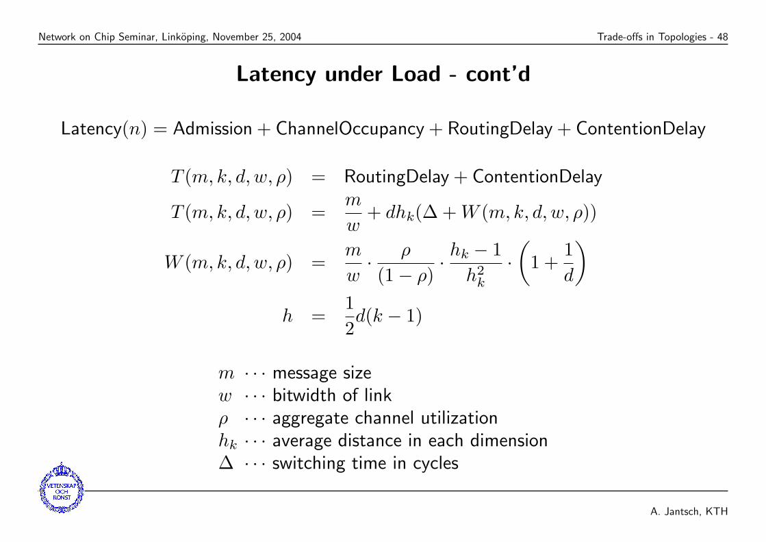
Latency(n) = Admission + ChannelOccupancy + RoutingDelay + ContentionDelay

T (m, k, d, w, ρ) = RoutingDelay + ContentionDelay

T (m, k, d, w, ρ) =m

w+ dhk(∆ + W (m, k, d, w, ρ))

W (m, k, d, w, ρ) =m

w· ρ

(1− ρ)· hk − 1

h2k

·(

1 +1d

)h =

12d(k − 1)

m · · · message sizew · · · bitwidth of linkρ · · · aggregate channel utilizationhk · · · average distance in each dimension∆ · · · switching time in cycles

A. Jantsch, KTH


Latency vs Channel Load

0

50

100

150

200

250

300

0 0.1 0.2 0.3 0.4 0.5 0.6 0.7 0.8 0.9 1

Ave

rage

late

ncy

Channel utilization

Latency wrt channel utilization (w=8;delta=1)

m8,d3,k10m8,d2,k32

m32,d3,k10m32,d2,k32

m128,d3,k10m128,d2,k32

A. Jantsch, KTH

Network on Chip Seminar, Linkoping, November 25, 2004 Routing - 50

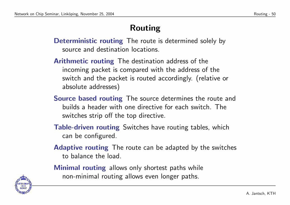
Routing

Deterministic routing The route is determined solely bysource and destination locations.

Arithmetic routing The destination address of theincoming packet is compared with the address of theswitch and the packet is routed accordingly. (relative orabsolute addresses)

Source based routing The source determines the route andbuilds a header with one directive for each switch. Theswitches strip off the top directive.

Table-driven routing Switches have routing tables, whichcan be configured.

Adaptive routing The route can be adapted by the switchesto balance the load.

Minimal routing allows only shortest paths whilenon-minimal routing allows even longer paths.

A. Jantsch, KTH


Deadlock

Deadlock Two or several packetsmutually block each other andwait for resources, which cannever be free.

Livelock A packet keeps movingthrough the network but neverreaches its destination.

Starvation A packet never gets aresource because it alwayslooses the competition for thatresource (fairness).

A. Jantsch, KTH


Deadlock Situations

• Head-on deadlock;

• Nodes stop receiving packets;

• Contention for switch buffers can occur withstore-and-forward, virtual-cut-through and wormholerouting. Wormhole routing is particularly sensible.

• Cannot occur in butterflies;

• Cannot occur in trees or fat trees if upward and downwardchannels are independent;

• Dimension order routing is deadlock free on k-ary n-arraysbut not on tori with any n ≥ 1.

A. Jantsch, KTH


Deadlock in a 1-dimensional Torus

Message 1 from C−> B, 10 flitsMessage 2 from A−> D, 10 flits

A B C D

A. Jantsch, KTH


Channel Dependence Graph for Dimension Order Routing

032

121

032

121

032

121

032

121

18 17

16 19

17 18

18 17

16 19

17 18

18 17

16 19

17 18

18 17

16 19

17 18

1 2 3

012

16

17

18

18

19

channel dependence graph

4−ary 2−array

17 17

18

19

Routing is deadlock free if the channel dependence graph has no cycles.

A. Jantsch, KTH


Deadlock-free Routing

• Two main approaches:

? Restrict the legal routes;

? Restrict how resources are allocated;

• Number the channel cleverly

• Construct the channel dependence graph

• Prove that all legal routes follow a strictly increasing pathin the channel dependence graph.

A. Jantsch, KTH


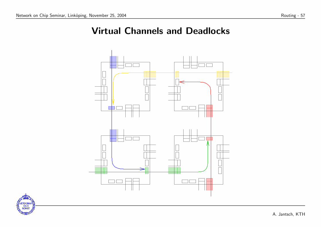
Virtual Channels

virtual channelsinputports

outpoutports

crossbar

• Virtual channels can be used to break cycles in thedependence graph.

• E.g. all n-dimensional tori can be made deadlock freeunder dimension-order routing by assigning allwrap-around paths to a different virtual channel thanother links.

A. Jantsch, KTH


Virtual Channels and Deadlocks

A. Jantsch, KTH


Turn-Model Routing

What are the minimal routing restrictions to make routing deadlock free?

North−last West−first Negative−first

• Three minimal routing restriction schemes:

? North-last

? West-first

? Negative-first

• Allow complex, non-minimal adaptive routes.

• Unidirectional k-ary n-cubes still need virtual channels.

A. Jantsch, KTH


Adaptive Routing

• The switch makes routing decisions based on the load.

• Fully adaptive routing allows all shortest paths.

• Partial adaptive routing allows only a subset of theshortest path.

• Non-minimal adaptive routing allows also non-minimalpaths.

• Hot-potato routing is non-minimal adaptive routingwithout packet buffering.

A. Jantsch, KTH

Network on Chip Seminar, Linkoping, November 25, 2004 Summary - 60

Summary

• Communication Performance: bandwidth, unloaded latency, loadedlatency

• Organizational Structure: NI, switch, link

• Topologies: wire space and delay domination favors low dimensiontopologies;

• Routing: deterministic vs source based vs adaptive routing;deadlock;

A. Jantsch, KTH

Network on Chip Seminar, Linkoping, November 25, 2004 Summary - 61

Issues beyond the Scope of this Lecture

• Switch: Buffering; output scheduling; flow control;

• Flow control: Link level and end-to-end control;

• Power

• Clocking

• Faults and reliability

• Memory architecture and I/O

• Application specific communication patterns

• Services offered to applications; Quality of service

A. Jantsch, KTH

Network on Chip Seminar, Linkoping, November 25, 2004 NoC Examples - 62

NoC Research Projects

• Nostrum at KTH

• Æthereal at Philips Research

• Proteo at Tampere University of Technology

• SPIN at UPMC/LIP6 in Paris

• XPipes at Bologna U

• Octagon at ST and UC San Diego

A. Jantsch, KTH


To Probe Further - Books and Classic Papers

[Agarwal, 1991] Agarwal, A. (1991). Limit on interconnection

performance. IEEE Transactions on Parallel and Distributed Systems,

4(6):613–624.

[Culler et al., 1999] Culler, D. E., Singh, J. P., and Gupta, A. (1999).

Parallel Computer Architecture - A Hardware/Software Approach.

Morgan Kaufman Publishers.

[Dally, 1990] Dally, W. J. (1990). Performance analysis of k-ary n-cube

interconnection networks. IEEE Transactions on Computers, 39(6):775–

785.

[Duato et al., 1998] Duato, J., Yalamanchili, S., and Ni, L. (1998).

Interconnection Networks - An Engineering Approach. Computer

Society Press, Los Alamitos, California.

[Leighton, 1992] Leighton, F. T. (1992). Introduction to Parallel

Algorithms and Architectures. Morgan Kaufmann, San Francisco.

A. Jantsch, KTH

Documents

Communication Performance in Network-on-Chipspetel71/NoC/lecture-notes/lect1part2.pdfCommunication Performance in Network-on-Chips Axel Jantsch Royal Institute of Technology, Stockholm