Communication Problems? The Role of Parent-child

RUHRECONOMIC PAPERS

Communication Problems? The Role

of Parent-child Communication for

the Subsequent Health Behavior of

Adolescents

#547

Daniel AvdicTugba Büyükdurmus

Imprint

Ruhr Economic Papers

Published by

Ruhr-Universität Bochum (RUB), Department of EconomicsUniversitätsstr. 150, 44801 Bochum, Germany

Technische Universität Dortmund, Department of Economic and Social SciencesVogelpothsweg 87, 44227 Dortmund, Germany

Universität Duisburg-Essen, Department of EconomicsUniversitätsstr. 12, 45117 Essen, Germany

Rheinisch-Westfälisches Institut für Wirtschaftsforschung (RWI)Hohenzollernstr. 1-3, 45128 Essen, Germany

Editors

Prof. Dr. Thomas K. BauerRUB, Department of Economics, Empirical EconomicsPhone: +49 (0) 234/3 22 83 41, e-mail: [email protected]

Prof. Dr. Wolfgang LeiningerTechnische Universität Dortmund, Department of Economic and Social SciencesEconomics – MicroeconomicsPhone: +49 (0) 231/7 55-3297, e-mail: [email protected]

Prof. Dr. Volker ClausenUniversity of Duisburg-Essen, Department of EconomicsInternational EconomicsPhone: +49 (0) 201/1 83-3655, e-mail: [email protected]

Prof. Dr. Roland Döhrn, Prof. Dr. Manuel Frondel, Prof. Dr. Jochen KluveRWI, Phone: +49 (0) 201/81 49-213, e-mail: [email protected]

Editorial Offi ce

Sabine WeilerRWI, Phone: +49 (0) 201/81 49-213, e-mail: [email protected]

Ruhr Economic Papers #547

Responsible Editor: Volker Clausen

All rights reserved. Bochum, Dortmund, Duisburg, Essen, Germany, 2015

ISSN 1864-4872 (online) – ISBN 978-3-86788-625-3The working papers published in the Series constitute work in progress circulated to stimulate discussion and critical comments. Views expressed represent exclusively the authors’ own opinions and do not necessarily refl ect those of the editors.

Ruhr Economic Papers #547

Daniel Avdic and Tugba Büyükdurmus

Communication Problems? The

Role of Parent-child Communication

for the Subsequent Health

Behavior of Adolescents

Bibliografi sche Informationen

der Deutschen Nationalbibliothek

Die Deutsche Bibliothek verzeichnet diese Publikation in der deutschen National-bibliografi e; detaillierte bibliografi sche Daten sind im Internet über: http://dnb.d-nb.de abrufb ar.

http://dx.doi.org/10.4419/86788625ISSN 1864-4872 (online)ISBN 978-3-86788-625-3

Daniel Avdic and Tugba Büyükdurmus1

Communication Problems? The Role

of Parent-child Communication for

the Subsequent Health Behavior of

Adolescents

Abstract

We contribute to the literature on the determinants of socioeconomic health disparities by studying how the health behavior of adolescents may arise from the degree of communication between parent and child. Parent-child communication may function as a mediator between family background and subsequent poor health behavior, potentially reconciling previous mixed evidence on the relationship between child health and social status. Using data from a unique German child health survey we construct an index of parent-child communication quality by comparing responses to statements about the children’s well-being from both children and their parents. Applying the constructed communication measure in a continuous treatment empirical framework, allowing for estimation of non-linear eff ects, our results show that improved parent-child communication monotonously reduces the smoking prevalence of adolescents by as much as 70%, irrespective of social background. More complex relationships are found for risky alcohol consumption and abnormal body weight.

JEL Classifi cation: C31, D83, I12, I14, J13

Keywords: Child health; health behavior; communication; intergenerational transmission; socioeconomic inequality; continuous treatment eff ect

April 2015

1 Daniel Avdic, UDE and CINCH; Tugba Büyükdurmus, UDE, CINCH, RWI, and RUB. – We thank Per Johansson, Martin Karlsson, Stephanie von Hinke Kessler Scholder, Harald Tauchmann and seminar participants at the University of Duisburg-Essen, CINCH Academy 2014, 10th joint iHEA and ECHE Congress in Dublin and the 7th dggö Jahrestagung in Bielefeld for useful comments. Data provided by the Robert Koch Institute and fi nancial support from the Bundesministerium für Bildung und Forschung (BMBF) are gratefully acknowledged. – All correspondence to: Tugba Büyükdurmus, CINCH–Health Economics Research Center, Edmund- Körner-Platz 2, 45127 Essen, Germany, e-mail: [email protected]

1 Introduction

The health of children and adolescents has recently become a major concern in many coun-

tries (Currie et al., 2004). A leading example is the rapid growth in the prevalence of child

obesity which has spurred considerable debate among both policy-makers and researchers

(Lobstein et al., 2004). Other areas of health behavior studied among the young includes to-

bacco smoking (Tyas and Pederson, 1998; Engels et al., 1998; Anda et al., 1999; Simantov et al.,

2000), alcohol use (Petraitis et al., 1998; Settertobulte et al., 2001; Schulenberg and Maggs,

2002), sexual health (Morris et al., 1993; Tráen and Kvalem, 1996), cannabis use (Bauman and

Ennett, 1996; Bachman et al., 1998; Patton et al., 2002), and oral health (Honkala et al., 1990;

Addy et al., 1990). Policies targeted at reducing avoidable health problems related to indi-

vidual behavior as early as possible are likely to be a cost-efficient way to achieve long-term

improvements in public health (cf. European Commission, 2013).1

Closely related to general concerns about child health are the consequences of social in-

equalities in childhood on observed health disparities. A number of studies have found sig-

nificant relationships between children’s socioeconomic status and their subsequent health

outcomes (see e.g., Bradley and Corwyn, 2002; Newacheck et al., 2003). It has been estimated

that over 70% of the factors determining health lies outside of the scope of health services

and are instead attributed to demographic, social, economic and environmental conditions

(NHH, 2000). Children and adolescents from families of low socioeconomic position are

overrepresented with respect to many health problems, such as mortality, injury, prevalence

of diagnosed illness, height, BMI, self-rated health and risk behavior (Currie et al., 2012).

Drewnowski (2010) provides a concrete example of this relationship, finding that budget re-

strictions play a role in the over-representation of obesity among children with low-income

parents, as nutritious, and more expensive, food is unaffordable. Life-lasting health inequal-

ities can therefore arise from differences in early life conditions during which the basis for a

healthy lifestyle is formed (cf. Center on the Developing Child, 2010).

In contrast, Hanson and Chen (2007) reports in a recent literature review that the ev-

idence on the relation between social background and health is less robust in childhood1In particular, article (4) of the European Commission’s recommendation states that “Early intervention and

prevention are essential for developing more effective and efficient policies, as public expenditure addressingthe consequences of child poverty and social exclusion tends to be greater than that needed for intervening atan early age” (European Commission, 2013, p. 5).

4

than in adulthood. Furthermore, Wang (2001) reports substantial variation in the socioe-

conomic health gradient in a cross-country study. Importantly, as socioeconomic status is

a highly complex and multidimensional concept, but often empirically constructed using

broad indicators such as earnings, income, education or occupation, some researchers have

argued that the mixed evidence may be a consequence of a too crude definition (Dutton

and Levine, 1989). For example, Bianchi (2000) find that employed mothers tend to offset

their increased working hours by spending time with their children more intensively in their

free time, while other studies has found an opposite pattern (see e.g., Anderson et al., 2003).

Adler et al. (1994) reviewed a number of potential psychosocial and behavioral mechanisms

potentially explaining the association between social background and health, stressing the

complexity of the relationship and calling for more detailed analysis of mediating factors.

The aim of this paper is to analyze whether and to which extent the communication

quality between parents and their children may serve as such a link between socioeconomic

status and health behavior of adolescents. The motivation is intuitive: a well-functioning

communication in a family is characterized by a situation in which household members ob-

serve each other and listen to each others beliefs, attitudes and habits. Mental and social

support is a fundamental form of communication which contributes to the child’s personal-

ity, development and behavior in almost all contexts of life (see e.g., Kunkel et al., 2006). As

such, family communication should be a key factor influencing children’s later health be-

havior and mediate effects related to more traditional measures of a family’s socioeconomic

status, as family communication is most likely related to factors such as income and educa-

tion. The causal link between family communication and health has so far, to the best of our

knowledge, not received much attention among researchers.2

To evaluate the impact of parent-child communication on adolescent health behavior

we make use of a unique, nationally representative, German child health survey, which

includes comprehensive information on the physical and mental health status as well as de-

tailed information on socioeconomic characteristics for more than 17,000 children between

0 and 17 years (Kurth et al., 2008). We use the data to construct a measure of the qual-

ity of communication between parent and child, based on the response correspondence to

2Parent-child communication has previously been analyzed descriptively in, for example, Laursen andCollins (2004) and Williams et al. (2010). Furthermore, in a related strand of literature, the impact of parentalhealth behavior on child health has been studied in, for example, Snow Jones et al. (1999).

5

statements about the child’s life satisfaction asked to both parents and their children. We

use this information to measure how well parents know their children in six different cate-

gories; physical health, psychological health, self-esteem and their satisfaction with family,

friends and school. This, indirect, technique is motivated by an attempt to reduce the risk of

social desirability bias from more direct questions, such as self-reported family communi-

cation quality, where subjects may respond untruthfully because of a willingness to appear

socially correct (cf. Maccoby and Maccoby, 1954; Fisher, 1993; Johnston et al., 2014). We re-

late our constructed communication measure to a number of health behavioral outcomes

(smoking, alcohol consumption and body weight) and adjust for the impact of confounding

factors using a propensity score approach in a continuous treatment setting, as outlined in

Hirano and Imbens (2004).

Our results show that parent-child communication quality may strongly influence the

health behavior of adolescents, but it crucially depends on the specific outcome. In particu-

lar, our estimates imply a 70% reduction in smoking prevalence between the lower and the

upper support of the communication distribution. Communication seem to be less impor-

tant for body weight and, in particular, for risky alcohol consumption where no difference

between the groups could be distinguished after adjustment for confounding factors. How-

ever, analyzing over- and underweight separately reveals that overweight is inversely, and

significantly, related to parent-child communication, while underweight is not. Our find-

ings suggest that communication may be an important factor mediating the relationship

between family social background and subsequent health outcomes. Policies should there-

fore be directed towards counseling of families in order to encourage, in particular poorer,

household’s ability to establish well-functioning communication channels.

The remainder of this article proceeds as follows: Section two describes the data, the sta-

tistical methodology we apply to construct the communication index and the econometric

framework used to isolate the impact of communication. Section three presents the empiri-

cal results, beginning with a descriptive analysis and followed by estimation results from the

multivariate analysis. Finally, section four offers a summary together with some concluding

remarks.

6

2 Data and Econometric Specification

This section begins with a brief introduction to the data and sample we use for our empiri-

cal analysis followed by a more detailed explanation on how we construct our parent-child

communication measure from the data. We subsequently explain the econometric frame-

work and estimation strategy we apply to isolate the causal effect of communication on

health behavior.

2.1 Data

The data used in this study originates from the Robert Koch Institute and is collected for the

German Health Interview and Examination Survey for Children and Adolescents (KiGGS)

between 2003 and 2006 (Kurth et al., 2008). It is a nationally representative and comprehen-

sive survey on the health of children in Germany 0-17 years, totaling 17,641 individuals. The

data include detailed individual-level information on physical and mental well-being (in the

form of an extensive clinical health assessment), health-related behavior (such as diet and

tobacco and alcohol utilization) as well as a number of socioeconomic and demographic

characteristics, acquired through the means of a computer-assisted personal interviewing

(CAPI) technique.

The KiGGS dataset is unique due to its comparatively large sample size and wide-ranging

and detailed information on the health of children. For the aims of this study, one crucial

feature of the data is that it contains a series of statements about the child’s life satisfaction,

asked to both the child and their accompanying parent. For each of these statements, the

child and parent are jointly asked to indicate how applicable it is for them on scale from

one to four (“does not match” to “matches exactly”). We use the responses from these state-

ments to create our measure of parent-child communication by constructing an index of the

degree to which the answers correspond. The underlying idea of this approach is simple;

the better parents know their children, the higher should their responses correspond with

the answers from the children. The degree of correspondence should then serve as an indi-

cator for how well a parent know their child, or, in other words, as a proxy for the quality

of communication between them. Using this indirect measure of parent-child communica-

tion is also likely to avoid empirical problems arising from using more direct measures (e.g.,

7

self-reported parental communication quality) as parents may want to respond in a socially

desirable way and thereby introduce systematic measurement error into the analysis. (cf.

Maccoby and Maccoby, 1954; Fisher, 1993).3

We restrict our analysis to adolescents aged 11–17 since the statements used to construct

our communication measure are only available for these age groups. This leaves us with

approximately 5,000 children remaining in the sample. In total 24 statements concerning the

life satisfaction of the interviewed children are used to construct the parent-child commu-

nication quality measure (see Table A.1 in Appendix A for a complete list of the questions).

We apply the Mahalanobis distance metric to comprise the information from the questions

into a single index. Formally, the Mahalanobis distance is in our application defined as the

square root of the sum of the squared distances between the parent and child’s responses,

weighted by the variance of the responses,

d(xc, xp) =√(xc − xp)′S−1(xc − xp), (2.1)

where d(·, ·) is the communication index as a function of the response vectors for the (c)hild

and the (p)arent, respectively (i.e., xj = {xj1, xj

2, . . . xji , . . . , xj

N} for i = 1, . . . , 24; j = c, p),

weighted by the response covariance matrix, S. To normalize the range of d(·, ·) to lie within

the unit interval and to transform it into an increasing function of parent-child response

correspondence, we weight each distance value by the maximum distance and reduce this

modified value from one4. Figure 2.1 plots the resulting distribution of the communication

measure along with statistics of the distribution. As specific values of the communication

index does not have a clear interpretation we will relate our analyses to the the quantiles of

the communication distribution in most of what follows.

To analyze how the parent-child communication affect subsequent health behavior we

consider three specific behavioral outcomes; the prevalence of smoking (defined as whether

the individual reports smoking tobacco), the level of alcohol consumption (whether the in-

dividual reports a risky level of alcohol consumption5) and having an unhealthy diet (BMI

3None of the statements used to construct the communication index explicitly mentions the communicationbetween parent and child in the family. See Table A.1 in Appendix A.

4Denoting the maximum possible value of the Mahalanobis distance metric dmax = max d(xc, xp), ournormalized communication measure is dnorm(xc, xp) = 1 − (d(xc, xp)/dmax).

5According to the German Centre for Addiction Issues (DHS) risky alcohol consumption level for adults

8

outside of the normal range6). The outcomes are defined as binary indicators where a value

of zero and one indicates the healthy and unhealthy condition, respectively. In additional

analyses we also use further categorizations of these outcomes to investigate the sensitivity

of the classifications.

FIGURE 2.1.Distribution of the Constructed Communication Index

Variable StatisticsMin:p1:p10:p20:p30:p40:p50:p60:p70:p80:p90:p99:Max:Mean:

0.000 0.244 0.476 0.539 0.576 0.607 0.632 0.655 0.677 0.702 0.734 0.810 0.892 0.615

0.0

2.0

4.0

6.0

8.1

.12

.14

Frac

tion

min p1 p10 p20 p30 p40 p50 p60 p70 p80 p90 p99 max

0 .1 .2 .3 .4 .5 .6 .7 .8 .9 1Communication Measure

NOTE.— Data source: KiGGS study conducted by the Robert Koch Institute. The graph shows the distributionof the constructed communication index by applying the Mahalanobis distance measure (equation (2.1)) on 24separate questions about the well-being of the interviewed child asked to both the child and the accompanyingparent. The full set of questions used to construct the index are listed in Table A.1 in Appendix A.

Figure 2.2 illustrates box-plots of the communication index outcome marginal distribu-

tions by health behavior category. Specifically, the left plot in each panel pertains to the

healthy outcome and the right to the unhealthy outcome. The figure shows that the commu-

nication density is higher in the upper part of the distribution for non-smokers and children

of normal weight compared to smokers and children with abnormal weight, while no such

difference is discernible for children reporting risky and non-risky alcohol consumption,

is defined as an intake of more than 20 (30) grams per day, five times a week for women (men). (DHS, 2003).Relating this definition to adolescents in our data, we define risky alcohol consumption as reporting drinkingalcohol at least 2-4 times per week.

6Defining over- or underweight for children is different than for adults. The weight categories are definedbased on percentiles of the body mass index (BMI) of the Kromeyer-Hauschild reference system (Kromeyer-Hauschild et al., 2001). According to this definition, a child is considered overweight (underweight) if theyare above (below) the ninetieth (tenth) BMI percentile in its age-gender-class. Furthermore, extreme over-weight/adiposity (underweight/anorexia) is defined as being above (below) the 97th (3rd) BMI percentilewithin its age-gender-class. As the KiGGS data is representative for Germany we use the sample distributionto identify the cutoffs for the different weight categories.

9

respectively.

FIGURE 2.2.Box-plots of the Communication Index by Health Behavior Outcome

0.1

.2.3

.4.5

.6.7

.8.9

1C

omm

unic

atio

n M

easu

re

Non-Smoker Smoker

Smoking

0.1

.2.3

.4.5

.6.7

.8.9

1

Normal Weight Abnormal Weight

Weight

0.1

.2.3

.4.5

.6.7

.8.9

1

Normal Consumption Risky Consumption

Alcohol

NOTE.— Data source: KiGGS study conducted by the Robert Koch Institute. The graph shows box-plot figuresof the communication index distribution separately for each of the health behavioral outcomes considered inthe study. The left (right) plot in each panel indicates the distribution for the healthy (unhealthy) outcome. Thehorizontal line in the box indicates the median, the gray box the interquartile range and the whiskers the maximumand minimum values of the distributions, respectively.

In our econometric analysis we include a set of socioeconomic and demographic charac-

teristics to adjust for heterogeneity across families which may distort the simple relationship

between our communication measure and the health behavioral outcomes. Parent-child

communication quality may be related to, for example, the parents’ employment status, in-

come and educational attainment which are all likely to affect children’s subsequent health

behavior. Table 2.1 reports means, differences in means and standard deviations for the

healthy and unhealthy outcome, respectively, by health outcome category for a set of co-

variates; child gender and age, family income, whether the parents are smoking or are over-

weight, parent employment status and educational level, whether the children live with

both parents, and characteristics of the region in which they live. The table reveals some in-

teresting patterns; for example, smoking and abnormal weight prevalences are much higher

among parents whose child is a smoker or has abnormal weight. Occupational status also

matters; while drinking and smoking behavior seem to be more prevalent among children

with full-time working parents, the opposite seems to be true for the likelihood that the child

10

is over- or underweight. The last rows of the table report group averages in the communi-

cation measure. Children who are smokers or have abnormal weight have, on average,

significantly poorer communication compared to non-smokers and children with normal

weight, while no such statistically significant difference exists for the prevalence of risky

alcohol consumption.

TABLE 2.1.Descriptive Sample Statistics

Variables Smoking Weight Alcohol

No Yes Difference No Yes Difference No Yes Difference

Mother unhealthy 0.280 0.457 -0.178*** 0.435 0.504 -0.069*** – – –(0.007) (0.017) (0.017) (0.008) (0.014) (0.016) – – –

Father unhealthy 0.359 0.505 -0.146*** 0.410 0.495 -0.084*** – – –(0.008) (0.017) (0.018) (0.008) (0.014) (0.016) – – –

Age 13.476 15.444 -1.968*** 13.828 13.822 0.006 13.552 15.919 -2.367***(0.030) (0.046) (0.067) (0.032) (0.055) (0.064) (0.028) (0.048) (0.079)

Male 0.507 0.485 0.022 0.505 0.503 0.001 0.477 0.702 -0.225***(0.008) (0.017) (0.018) (0.008) (0.014) (0.016) (0.008) (0.019) (0.022)

Unemployed 0.235 0.224 0.012 0.223 0.264 -0.041*** 0.235 0.214 0.021(0.007) (0.014) (0.016) (0.007) (0.012) (0.014) (0.006) (0.017) (0.019)

Part-time employed 0.491 0.416 0.075*** 0.479 0.476 0.003 0.482 0.460 0.022(0.008) (0.016) (0.018) (0.008) (0.014) (0.016) (0.008) (0.021) (0.022)

Full-time employed 0.273 0.360 -0.087*** 0.300 0.261 0.037*** 0.283 0.327 -0.043***(0.007) (0.016) (0.017) (0.007) (0.012) (0.015) (0.007) (0.019) (0.020)

No occupation 0.082 0.102 -0.021*** 0.080 0.100 -0.020*** 0.087 0.069 0.018(0.004) (0.010) (0.010) (0.004) (0.009) (0.009) (0.004) (0.010) (0.012)

Occupation 0.457 0.574 -0.115*** 0.474 0.497 -0.023 0.474 0.519 -0.045***(0.008) (0.017) (0.018) (0.008) (0.014) (0.016) (0.008) (0.021) (0.022)

Graduate occupation 0.319 0.281 0.038*** 0.319 0.292 0.026* 0.316 0.290 0.027(0.007) (0.015) (0.017) (0.008) (0.013) (0.015) (0.007) (0.019) (0.020)

Living in a rural area 0.492 0.505 -0.013 0.494 0.496 -0.002 0.481 0.603 -0.121***(0.008) (0.017) (0.018) (0.008) (0.014) (0.016) (0.008) (0.020) (0.022)

Immigrant 0.119 0.086 0.033*** 0.112 0.117 -0.005 0.120 0.059 0.061***(0.005) (0.009) (0.012) (0.005) (0.009) (0.010) (0.005) (0.010) (0.014)

Number of children 2.378 2.885 -0.507*** 2.488 2.416 0.071 2.347 3.382 -1.035***(0.027) (0.073) (0.067) (0.030) (0.051) (0.060) (0.026) (0.094) (0.079)

Living with both parents 0.814 0.709 0.105*** 0.800 0.779 0.021 0.794 0.808 -0.014(0.006) (0.015) (0.015) (0.007) (0.017) (0.013) (0.006) (0.016) (0.018)

Living in West Germany 0.680 0.593 0.087*** 0.664 0.665 -0.001 0.663 0.677 -0.014(0.007) (0.016) (0.017) (0.008) (0.013) (0.015) (0.007) (0.019) (0.021)

Disposable income under 0.302 0.368 -0.066*** 0.300 0.355 0.055 0.315 0.300 0.019risk-of-poverty threshold (0.007) (0.016) (0.017) (0.007) (0.014) (0.015) (0.007) (0.019) (0.020)Disposable income above 0.513 0.498 0.014 0.521 0.480 0.041 0.507 0.540 -0.033*risk-of-poverty threshold (0.008) (0.017) (0.018) (0.008) (0.014) (0.016) (0.008) (0.021) (0.022)Disposable income above 0.185 0.134 0.052*** 0.179 0.166 0.014 0.178 0.163 0.015wealth-threshold (0.006) (0.011) (0.014) (0.006) (0.011) (0.012) (0.006) (0.015) (0.017)

Communication 0.620 0.591 0.028*** 0.617 0.607 0.010*** 0.614 0.620 -0.007(0.002) (0.004) (0.004) (0.002) (0.003) (0.004) (0.002) (0.005) (0.005)

NOTE.— Data source: KiGGS study conducted by the Robert Koch Institute. The table reports means (standard deviations) of covariatesincluded in the empirical analysis by the healthy and unhealthy outcome and their difference for each of the different health behaviorsamples; smoking prevalence, weight problems and risky alcohol consumption. Statistics of the constructed communication measure arelisted in boldface font at the bottom. Estimation of statistical significance is performed through a standard Wald test of equality of means.*, ** and *** denote significance at the 10, 5 and 1 percent levels. For detailed variable definitions, see Table A.2 in Appendix A.

2.2 Econometric framework

Table 2.1 showed that our constructed communication index is far from the only factor that

varies across the health behavioral outcomes considered in this study. Parental and family-

11

specific characteristics also affect children’s health behavior independently of the level of

communication between parent and child. Even though systematic measurement error in

the communication variable due to social desirability bias may not be an issue, correlations

of parent characteristics and parent-child communication could still distort the effect of com-

munication. To adjust for the influence of confounding factors in a continuous treatment

framework, we apply a generalized version of the classical binary treatment propensity

score matching approach (see e.g., Rosenbaum and Rubin, 1983), developed by Hirano and

Imbens (2004), to estimate a dose-response function which allows us to evaluate the effect

of communication across the whole distribution of the communication variable. Hence, in

contrast to the classical binary treatment approach, we are able to estimate non-linear effects

and analyze the causal relationship between parent-child communication and adolescent

health behavior in more detail.

To briefly set the stage for our empirical approach we borrow the potential outcomes

framework setup from Hirano and Imbens (2004). Consider our sample of i = 1, ..., N chil-

dren for which we observe one realized outcome, Yi = Yi(Ci), from a set of potential out-

comes, Yi(c), where c ∈ C is our index of parent-child communication. In the binary case we

could define communication as either “good” or “bad”, C = {bad, good}, according to some

assignment mechanism and apply the binary treatment propensity score matching frame-

work. However, since our communication measure is an interval over [cmin, cmax], a more

general and informative approach would be to estimate the (average) marginal effect7 of in-

creasing communication between a parent and her child, say from ct to ct+1, on subsequent

behavioral outcomes,

μct+1,ct = E[Yi(ct+1)]− E[Yi(ct)], (2.2)

where E[Yi(c)] is the average dose-response function conditional on receiving communica-

tion level c and μct+1,ct is the treatment effect. Hirano and Imbens (2004) shows that this

parameter can be consistently estimated under the assumption that, conditional on a set of

covariates X, the level of communication received by each child is independent of the po-

tential health behavior outcome for each value of the treatment, Y(c) ⊥ C | X ∀ c ∈ C. This

7As the communication interval is discretized in the estimation of the marginal treatment effect (see below)the estimated effect is, in practice, the average marginal effect within each communication bin. However, sincewe also estimate average treatment effect in a binary treatment setting we decided to exclude the “average”part from the continuous treatment framework terminology hereinafter to avoid confusion.

12

is a direct generalization of the original Rosenbaum and Rubin (1983) unconfoundedness

assumption.

To adjust for confounding factors we estimate the generalized propensity score (GPS),

Ri = r(Ci, Xi), defined as the conditional density of received communication level given co-

variates X. The analogy to the binary treatment propensity score framework is that, rather

than only balancing the covariates across children having a “good” or “bad” communication

level with their parents, the corresponding balancing property for the GPS is that treatment

assignment should be randomly distributed within each strata of r(c, X). Hence, applica-

tion of the GPS under the unconfoundedness assumption makes it possible to consistently

estimate the dose-response function and, consequently, the marginal treatment effects over

the entire support of the parent-child communication index.

In practice, the covariate-adjusted dose-response function is estimated in two steps. We

first estimate the conditional expectation of the outcome of interest as a function of the

GPS and the realized level of communication. Next, the estimated parameters from this

model are used to estimate the conditional expectation evaluated at each communication

level separately. We specify a flexible polynomial and estimate the parameters by ordinary

least squares. The communication measure is discretized into ten categories defined by the

deciles of its distribution, i.e., C = {cq1, cq2, ..., cq9, ..., , cq10}, where cq1 < pc(10) ≤ cq2 <

pc(20)... ≤ cq9 < pc(90) ≤ cq10.

To estimate the GPS we first apply a standard probit estimated by maximum likelihood,

Pr(c = Ci|Xi) = φ(α0 + X′iα1)

−1, (2.3)

and then predict Ri using the estimated parameters from this equation. For the dose-response

function we first estimate the quadratic function,

E[Yi|Ci, Ri] = β0 + β1Ci + β2C2i + β3Ri + β4R2

i + β5(Ci × Ri), (2.4)

and then use the estimated parameters from this model to estimate the dose response func-

13

tion evaluated at the specific communication level, c, by plugging in the predicted GPS,

E[Y(c)] = β0 + β1c + β2c2 + β3r(c, Xi) + β4r(c, Xi)2 + β5(c × r(c, Xi)). (2.5)

Carrying out this procedure for each communication interval we are able estimate the dose-

response function over the whole communication distribution and compute μct,ct+1 for each

(ct, ct+1) pair.

Finally, to relate the GPS results to the binary treatment framework we also apply a stan-

dard nearest neighbor propensity score matching approach where we use different quantiles

of the communication index distribution to assign children to good and bad parent-child

communication levels. This corresponds approximately to estimating the marginal effect of

communication for the same cutoffs in the continuous framework. That is, integrating over

the relevant part of the marginal treatment effect distribution we can recover the average

treatment effect for the specific assignment cutoff values. Denoting T = 1(c > x) the as-

signment equation with cutoff x, the average treatment effect as ATET1,T0 and the marginal

treatment effect as MTEct+1,ct , we have,

ATET1,T0 =∫ ∞

xMTE(c)dc −

∫ x

−∞MTE(c)dc. (2.6)

We use the median and the first and fourth quartiles of the communication index as

treatment cutoffs. Since the latter assignment scheme compares more extreme individu-

als with respect to the parent-child communication, we expect that this comparison would

yield a stronger effect than the median cutoff comparison if the effect of communication is

monotone in the outcomes we consider. Taken together, comparing the results from both

approaches could yield further insights into the mechanics of the effect.

3 Results

In this section we present the empirical results of the relation between parent-child commu-

nication level and the health behavioral outcomes we consider. We begin by presenting some

initial descriptive evidence of the relationship before turning to the multivariate propensity

14

score matching framework.

3.1 Descriptive analysis

Figure 3.1 illustrates the marginal outcome distributions of our constructed communica-

tion index for each of the three behavioral categories we consider; tobacco smoking, body

weight and alcohol consumption. The left and right panels plot the cumulative and prob-

ability density functions, respectively, where the latter are fitted using a Gaussian kernel

smoothing function. Finally, the short dashed lines indicate the quantile-specific differences

in the communication measure between the marginal distributions.

FIGURE 3.1.Distribution of Communication Index by Health Behavioral Outcome

.01

.02

.03

.04

.05

Qua

ntile

Gro

up D

iffer

ence

0.1

.2.3

.4.5

.6.7

.8.9

1C

DF(

Com

mun

icat

ion)

0 .1 .2 .3 .4 .5 .6 .7 .8 .9 1Communication Quantile

0 .1 .2 .3 .4 .5 .6 .7 .8 .9Communication Measure

Not SmokerSmokerDifference

Cumulative Distribution

0.5

11.

52

2.5

33.

54

4.5

Den

sity


Not SmokerSmoker

Kernel Density Estimate

Smoking

-.01

0.0

1.0

2.0

3Q

uant

ile G

roup

Diff

eren

ce

0.1

.2.3

.4.5

.6.7

.8.9

1C

DF(

Com

mun

icat

ion)



Normal WeightAbnormal WeightDifference


0.5

11.

52

2.5

33.

54

4.5

Den

sity


Normal WeightAbnormal Weight


Weight

-.02

-.01

0.0

1.0

2Q

uant

ile G

roup

Diff

eren

ce

0.1

.2.3

.4.5

.6.7

.8.9

1C

DF(

Com

mun

icat

ion)



Normal ConsumptionRisky ConsumptionDifference


0.5

11.

52

2.5

33.

54

4.5

Den

sity


Normal ConsumptionRisky Consumption


Alcohol

NOTE.— Data source: KiGGS study conducted by the Robert Koch Institute. The figure depicts the cumula-tive (left panel) and kernel-estimated probability density (right panel) marginal distributions of the constructedcommunication index by the healthy and unhealthy outcome and their difference for each of the different healthbehavior samples; smoking prevalence, weight problems and risky alcohol consumption. The dotted line in theright panels indicate the quantile-specific difference in communication between the healthy and unhealthy behav-ioral outcome.

The figure shows that the healthy outcome (non-smoker, normal body weight and safe

alcohol consumption) stochastically dominates the unhealthy outcomes (smoker, abnormal

body weight and risky alcohol consumption) in the two first cases while the result for the

alcohol category is ambiguous. In particular, the healthy outcome seem to dominate for al-

cohol consumption in the lower and middle part of the communication distribution but the

15

relationship becomes inverted in the upper part. The pattern is also visible in the kernel

density functions where the healthy outcomes are shifted to the right for the smoking and

weight categories but not for alcohol consumption. In general, differences in the commu-

nication measure are greatest in the lower part of the distributions; around .03 and .05 for

the weight and smoking outcomes, corresponding to between .5 and 1 standard deviations,

respectively. This descriptive evidence hence suggest that variation in adolescents’ health

behaviors arise primarily at the lower end of the communication distribution.

To further explore the relation between the communication measure and the behavioral

outcomes, Figure 3.2 displays percentile-specific shares of sampled individuals with the un-

healthy outcome for each behavioral category together with a locally smoothed regression

trend. Again, the descriptive evidence tells us that a higher communication level is related

to a lower prevalence of smokers and abnormal body weight, while the relation is less clear

for risky alcohol consumption. In particular, the difference in smoking prevalence between

the upper and lower part of the communication distribution is approximately 50%, while

substantially lower for the two other behavioral categories (15% and 10% for the alcohol

and weight outcomes, respectively).

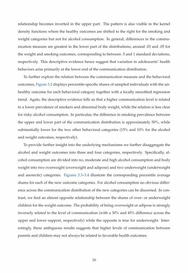
To provide further insight into the underlying mechanisms we further disaggregate the

alcohol and weight outcomes into three and four categories, respectively. Specifically, al-

cohol consumption are divided into no, moderate and high alcohol consumption and body

weight into two overweight (overweight and adipose) and two underweight (underweight

and anorectic) categories. Figures 3.3–3.4 illustrate the corresponding percentile average

shares for each of the new outcome categories. For alcohol consumption no obvious differ-

ence across the communication distribution of the new categories can be discerned. In con-

trast, we find an almost opposite relationship between the shares of over- or underweight

children for the weight outcome. The probability of being overweight or adipose is strongly

inversely related to the level of communication (with a 30% and 45% difference across the

upper and lower support, respectively) while the opposite is true for underweight. Inter-

estingly, these ambiguous results suggests that higher levels of communication between

parents and children may not always be related to favorable health outcomes.

16

FIGURE 3.2.Communication Index Quantile Averages by Health Behavioral Outcome

0.0

5.1

.15

.2.2

5.3

.35

.4.4

5.5

Sha

re S

mok

ers


Average Local smooth 95% confidence band

Smoking

0.0

5.1

.15

.2.2

5.3

.35

.4.4

5.5

Sha

re A

bnor

mal

Wei

ght



Weight

0.0

5.1

.15

.2.2

5.3

.35

.4.4

5.5

Sha

re R

isky

Alc

ohol

Con

sum

ptio

n



Alcohol

NOTE.— Data source: KiGGS study conducted by the Robert Koch Institute. The figure depicts the communica-tion quantile-average share of individuals with the unhealthy outcome for each of the different health behaviorsamples; smoking prevalence, weight problems and risky alcohol consumption. The solid line in each panel indi-cates the relationship estimated using a local polynomial regression smoother and the gray area its corresponding95% confidence interval.

FIGURE 3.3.Communication Index Quantile Averages by Health Behavioral Outcome: Alcohol

Categories

0.0

5.1

.15

.2.2

5.3

.35

.4.4

5.5

.55

.6.6

5S

hare

No

Alc

ohol

Con

sum

ptio

n



No Alcohol Consumption

0.0

5.1

.15

.2.2

5.3

.35

.4.4

5.5

.55

.6.6

5S

hare

Mod

erat

e A

lcoh

ol C

onsu

mpt

ion



Moderate Alcohol Consumption

0.0

5.1

.15

.2.2

5.3

.35

.4.4

5.5

.55

.6.6

5S

hare

Hig

h A

lcoh

ol C

onsu

mpt

ion



High Alcohol Consumption

NOTE.— Data source: KiGGS study conducted by the Robert Koch Institute. The figure depicts the communica-tion quantile-average share of individuals for an alternative categorization of the alcohol outcome. See the textfor category definitions. The solid line in each panel indicates the relationship estimated using a local polynomialregression smoother and the gray area its corresponding 95% confidence interval.

17

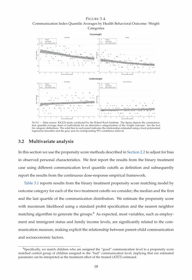
FIGURE 3.4.Communication Index Quantile Averages by Health Behavioral Outcome: Weight

Categories

0.0

5.1

.15

.2.2

5.3

Sha

re O

verw

eigh

t



Overweight

0.0

5.1

.15

.2.2

5.3

Sha

re A

dipo

se



Adipose

Overweight0

.05

.1.1

5.2

.25

Sha

re U

nder

wei

ght



Underweight

0.0

5.1

.15

.2.2

5S

hare

Ano

rect

ic



Anorexia Nervosa

Underweight

NOTE.— Data source: KiGGS study conducted by the Robert Koch Institute. The figure depicts the communica-tion quantile-average share of individuals for an alternative categorization of the weight outcome. See the textfor category definitions. The solid line in each panel indicates the relationship estimated using a local polynomialregression smoother and the gray area its corresponding 95% confidence interval.

3.2 Multivariate analysis

In this section we use the propensity score methods described in Section 2.2 to adjust for bias

in observed personal characteristics. We first report the results from the binary treatment

case using different communication level quantile cutoffs as definition and subsequently

report the results from the continuous dose-response empirical framework.

Table 3.1 reports results from the binary treatment propensity score matching model by

outcome category for each of the two treatment cutoffs we consider; the median and the first

and the last quartile of the communication distribution. We estimate the propensity score

with maximum likelihood using a standard probit specification and the nearest neighbor

matching algorithm to generate the groups.8 As expected, most variables, such as employ-

ment and immigrant status and family income levels, are significantly related to the com-

munication measure, making explicit the relationship between parent-child communication

and socioeconomic factors.

8Specifically, we match children who are assigned the “good” communication level to a propensity scorematched control group of children assigned to the “bad” communication level, implying that our estimatedparameter can be interpreted as the treatment effect of the treated (ATET) estimand.

18

TABLE 3.1.Results from Propensity Score Estimation by Outcome Category and Treatment Definition

Communication Communication

(Median Threshold) (1st vs 4th Quartile Threshold)

Smoking Weight Alcohol Smoking Weight Alcohol

Mother unhealthy -0.074 -0.093* – -0.162* -0.131* –(0.040) (0.036) – (0.060) (0.052) –

Father unhealthy -0.108** -0.064 – -0.115* -0.122* –(0.040) (0.037) – (0.060) (0.054) –

Age 0.021* 0.020* 0.020* 0.017 0.019 0.020(0.011) (0.009) (0.011) (0.013) (0.014) (0.016)

Unemployed -0.113* -0.108* -0.117* -0.198** -0.187** -0.197**(0.054) (0.046) (0.056) (0.071) (0.068) (0.072)

Full-time employed 0.013 -0.001 -0.004 -0.073 -0.108 -0.111(0.054) (0.055) (0.055) (0.071) (0.072) (0.071)

No occupation -0.233** -0.246*** -0.252*** -0.401*** -0.422*** -0.424***(0.072) (0.071) (0.073) (0.117) (0.119) (0.116)

Graduate occupation 0.079* 0.090** 0.104** 0.140** 0.139** 0.167***(0.043) (0.041) (0.041) (0.062) (0.061) (0.060)

Immigrant -0.605*** -0.607*** -0.607*** -0.854*** -0.834*** -0.837***(0.071) (0.072) (0.068) (0.094) (0.093) (0.094)

Number of children 0.013 0.017 0.017 0.017 0.021 0.020(0.011) (0.012) (0.011) (0.021) (0.022) (0.021)

Living in West -0.043 -0.028 -0.030 -0.058 -0.047 -0.048Germany (0.046) (0.045) (0.042) (0.067) (0.066) (0.067)Living with both parents 0.108* 0.155*** 0.170*** 0.205** 0.225** 0.262***

(0.055) (0.054) (0.054) (0.075) (0.078) (0.077)Disposable income under -0.171*** -0.171*** -0.177*** -0.311*** -0.307*** -0.315***risk-of-poverty threshold (0.041) (0.041) (0.043) (0.064) (0.064) (0.065)Disposable income above 0.146** 0.148** 0.151** 0.222** 0.211** 0.214**wealth threshold (0.053) (0.056) (0.056) (0.082) (0.081) (0.071)

Observations 4886 5074 5074 2432 2537 2537

NOTE.— Data source: KiGGS study conducted by the Robert Koch Institute. The table reports parameter point estimates (standarderrors) from the estimation of the matching propensity score using the probit model specification from equation (2.3) and the maximumlikelihood estimator for each health behavior sample (smoking, weight and alcohol) and by treatment assignment cutoff (median and thefirst and fourth quartile) of the communication index distribution. Robust standard errors in parentheses are clustered at the individuallevel. *, ** and *** denote significance at the 10, 5 and 1 percent levels. For detailed variable definitions, see Table A.2 in Appendix A.

Table 3.2 reports the covariate balancing results from matching on the smoking preva-

lence outcome by treatment cutoff (matching results for the two other outcomes are listed in

Tables A.3–A.4 in Appendix A). The second column in the table specify whether the sample

considered is the unmatched or matched sample. For each treatment cutoff, the first two

columns reports the conditional means given the assigned communication level, and the

last two columns report the percent bias reduction between the unmatched and matched

sample and the p-value from a test of the difference between the means, respectively. As

can be seen from the table, the matching algorithm is successful in balancing the covariates

across the groups and the test for the equality of means cannot be rejected for any of the

variables included. Similar results are obtained for the two other behavioral outcomes.

19

TABLE 3.2.Covariate Balancing Results from Propensity Score Matching: Smoking Outcome



E[X|c = C] SB red. E[X|c = C] SB red.Sample Good Bad in % p-value Good Bad in % p-value

Mother unhealthy U 0.275 0.327 0.000 0.251 0.341 0.000M 0.275 0.270 90.6 0.701 0.251 0.250 99.1 0.963

Father unhealthy U 0.344 0.426 0.000 0.346 0.460 0.000M 0.344 0.339 93.5 0.696 0.346 0.339 93.5 0.701

Age U 13.904 13.745 0.005 13.903 13.768 0.101M 13.904 13.913 94.6 0.879 13.903 13.939 73.2 0.659

Unemployed U 0.198 0.265 0.000 0.182 0.291 0.000M 0.198 0.185 79.7 0.232 0.182 0.181 99.3 0.958

Full-time employed full U 0.303 0.271 0.014 0.304 0.282 0.221M 0.303 0.300 92.3 0.852 0.304 0.317 45.8 0.512

No occupation U 0.050 0.119 0.000 0.040 0.155 0.000M 0.050 0.047 94.7 0.551 0.040 0.040 100.0 1.000

Graduate occupation U 0.350 0.279 0.000 0.376 0.260 0.000M 0.350 0.334 77.7 0.241 0.376 0.353 80.2 0.239

Immigrant U 0.058 0.168 0.000 0.052 0.237 0.000M 0.058 0.057 98.9 0.854 0.052 0.040 93.8 0.176

Number of children U 2.498 2.478 0.691 2.528 2.522 0.936M 2.498 2.463 -70.1 0.491 2.528 2.617 -1356.9 0.223

Living in West U 0.649 0.684 0.010 0.651 0.691 0.040Germany M 0.649 0.643 82.5 0.655 0.651 0.703 -31.4 0.006Living with both parents U 0.832 0.800 0.004 0.854 0.798 0.000

M 0.832 0.855 26.0 0.023 0.854 0.869 74.0 0.292Disposable income under U 0.250 0.367 0.000 0.224 0.421 0.000risk-of-poverty threshold M 0.250 0.260 91.9 0.452 0.224 0.243 90.4 0.272Disposable income above U 0.213 0.140 0.000 0.227 0.115 0.000wealth threshold M 0.213 0.188 65.3 0.027 0.227 0.213 87.5 0.406

Observations 4860 2418

NOTE.— Data source: KiGGS study conducted by the Robert Koch Institute. The table reports balancing results of included covariatesbefore and after propensity score matching (rows U and M) for the smoking behavioral sample by treatment status. Treatment status(“Good”,“Bad”) is determined by the respective treatment assignment cutoff of the communication index distribution (median and thefirst and fourth quartile, respectively). The third and fourth columns of each cutoff category indicates the percentage reduction in thedifference of the means between the unmatched and matched samples and the p-value from a standard Wald test of difference in meansacross the treatment categories, respectively. For detailed variable definitions, see Table A.2 in Appendix A.

Given the successful balancing of the covariates we now move on to present the results

of the effect of communication on the behavioral outcomes. The upper and lower panel of

Table 3.3 report the results for the median and the first and the last quartile treatment cut-

offs, respectively. Once again, we present the results for both the unmatched and matched

samples, indicated in column two, followed by the estimated conditional means for each of

the two potential outcomes and their difference, the treatment effect. The last two columns

of the table report the standard error and significance level of the effect.

First, it is interesting to note that matching attenuates the effect of communication for

both the alcohol and the weight outcomes while, in contrast, accentuates the effect on smok-

ing prevalence. The latter is highly significant while the effect of communication on alcohol

seem to be completely driven by the covariates and is close to zero after the matching. The

effect on the weight outcome drops and becomes insignificant after covariate adjustment.

However, this result seem to be primarily driven by reduced statistical precision.

20

The magnitude of the effects are substantial for the weight and, in particular, the smok-

ing outcomes. The effect for the median cutoff implies a change in the prevalence of smok-

ing and abnormal weight of 35%(.075/.218

)and 12%

(.031/.263), respectively. This difference

increases to 48% and 14% when comparing the two more extreme groups in the first and

fourth quartile of the communication index distribution. The difference in the prevalence of

risky alcohol consumption is close to zero for both cutoffs, indicating no important effect of

communication in this dimension.

TABLE 3.3.Estimated Average Treatment Effect of the Treated by Outcome and Treatment Definition

Outcome Sample E[Y(G)] E[Y(B)] E[Y(G)− E[Y(B)] Std. Err. p-value

Panel A: Treatment Definition – Median ThresholdSmoking U 0.144 0.209 -0.065 0.011*** <0.001

M 0.144 0.218 -0.075 0.019*** <0.001Weight U 0.231 0.268 -0.036 0.012*** 0.003

M 0.231 0.263 -0.031 0.019 0.110Alcohol U 0.127 0.109 0.019 0.009** 0.038

M 0.127 0.116 0.012 0.019 0.542

Panel B: Treatment Definition – 1st vs 4th Quartile ThresholdSmoking U 0.121 0.229 -0.108 0.015*** <0.001

M 0.121 0.233 -0.112 0.027*** <0.001Weight U 0.232 0.278 -0.046 0.017*** 0.008

M 0.232 0.271 -0.039 0.028 0.153Alcohol U 0.135 0.108 0.028 0.013** 0.033

M 0.135 0.134 0.002 0.024 0.944

NOTE.— Data source: KiGGS study conducted by the Robert Koch Institute. The table reports the estimated conditional means giventhe treatment status (“Good”,“Bad”) and their difference (the average treatment effect) for (U)nmatched and propensity score (M)atchedsamples for each health behavior outcome; smoking prevalence, weight problems and risky alcohol consumption. Treatment status(“Good”,“Bad”) is determined by the respective treatment assignment cutoff of the communication index distribution (median and thefirst and fourth quartile, respectively) and shown in panels A and B of the table, respectively. The two last columns indicate the standarderrors of the treatment effect and the respective p-value of a standard Wald test of equality of the conditional means. *, ** and *** denotesignificance at the 10, 5 and 1 percent levels.

As the results of the weight outcome were inconclusive we ran additional analyses for

the over- and underweight categories separately. Results from this exercise are reported in

Table 3.4 and largely confirms the earlier pattern from Figure 3.4. In particular, the effect

of communication on the probability that a child is overweight is strongly negative and

statistically significant, while the results for underweight go in the opposite direction. The

former estimate implies approximately a 25% increased risk of overweight if the child had

a poor, rather than a good, communication with their parent. The reversed relationship

between communication and underweight is curious but could reflect a situation in which,

for example, overly worried parents induce unhealthy dietary stress in their children, as

they may consider underweight less of a health risk than overweight.

21

TABLE 3.4.Estimated Average Treatment Effect of the Treated for Subcategories of the Weight Outcome

Outcome Sample E[Y(G)] E[Y(B)] E[Y(G)− E[Y(B)] Std. Err. p-value

Treatment: Median ThresholdOverweight U 0.122 0.181 -0.058 0.010*** <0.001

M 0.122 0.163 -0.041 0.018** 0.024Underweight U 0.109 0.087 0.022 0.008*** 0.008

M 0.109 0.095 0.015 0.015 0.342

Treatment: 1st vs 4th Quartile ThresholdOverweight U 0.115 0.196 -0.081 0.014*** <0.001

M 0.115 0.160 -0.045 0.026* 0.082Underweight U 0.117 0.081 0.035 0.012*** 0.003

M 0.117 0.085 0.032 0.020 0.107

NOTE.— Data source: KiGGS study conducted by the Robert Koch Institute. The table reports the estimated conditional means giventhe treatment status (“Good”,“Bad”) and their difference (the average treatment effect) for (U)nmatched and propensity score (M)atchedsamples for subcategories of the weight behavioral outcome. Treatment status (“Good”,“Bad”) is determined by the respective treatmentassignment cutoff of the communication index distribution (median and the first and fourth quartile, respectively) and shown in panelsA and B of the table, respectively. The two last columns indicate the standard errors of the treatment effect and the respective p-value of astandard Wald test of equality of the conditional means. *, ** and *** denote significance at the 10, 5 and 1 percent levels.

We now proceed with analyzing the dose-response relationship between our communi-

cation index and the behavioral outcomes using the continuous treatment framework. To

briefly explain how the results from the binary and continuous treatment approaches are

related, Figure 3.5 combine the binary treatment effect results from Table 3.3 and the esti-

mated dose-response function for the smoking outcome. The long dashed line indicates the

dose-response function for each the treatment level (i.e., communication quantile) and the

gray area around the line is a 95% confidence band of this estimate. The dot-dashed line,

scaled by the right y-axis, shows the marginal treatment effect of increasing communication

from c to c + 1 (i.e., the derivative of the dose-response function). Finally, the horizontal

lines indicate the conditional means for the two separate treatment cutoff definitions in the

binary treatment model, with their corresponding differences, the average treatment effects,

calculated in the small upper right text box in the figure. As can be seen, the conditional

means are weighted averages of the dose-response relationship and the average treatment

effects are weighted averages of the marginal treatment effects across the relevant parts of

the communication distribution. Hence, the additional information provided by the con-

tinuous treatment framework allows us to analyze heterogeneity and non-linearities in the

effect of communication more in detail.

22

FIGURE 3.5.Detailed analysis of the Effects of Communication on Smoking Behavior

Q1 Q2 Q3 Q4

E[Y(B)]Median=0.218

E[Y(G)]Median=0.144

E[Y(B)]Q4-Q1=0.233

E[Y(G)]Q4-Q1=0.121

ATETMedian=0.144-0.218=-0.075ATETQ4-Q1=0.121-0.233=-0.112

-.025

-.02

-.015

-.01

-.005

E[S

mok

er(c

+1) -

Sm

oker

(c)]

.05

.1.1

5.2

.25

.3E

[Sm

oker

(c)]

0 .1 .2 .3 .4 .5 .6 .7 .8 .9 1Communication Quantile (c)

Dose-Response95% confidence bandMarginal Treatment EffectAverage Treatment Effect (Median)Average Treatment Effect (Q4-Q1)

Dose-Response Function: Smoking Outcome

NOTE.— Data source: KiGGS study conducted by the Robert Koch Institute. The figure depicts the combinedresults from applying the nearest neighbor binary propensity matching and continuous treatment generalizedpropensity score estimation methodology suggested by Hirano and Imbens (2004) for the smoking behavioraloutcome. See Section 2.2 for estimation details. The long dashed line indicates the dose-response function con-ditional on the communication quantile together with a 95% confidence interval. The short dashed line showsthe corresponding estimated marginal treatment effect conditional on the communication quantile, defined as thedifference in the estimated dose-response between treatment level c + 1 and c. The horizontal lines show thecorresponding conditional means as reported in Table 3.3 for the respective treatment assignment cutoff of thecommunication index distribution (median and the first and fourth quartile, respectively).

Figure 3.6 show the dose-response function and the associated marginal treatment effects

for each health behavior category separately. If the effect of parent-child communication is

monotonously reducing unhealthy behavior, the latter should always be below zero. How-

ever, as we can see from the figure, this is only the case for the smoking outcome. The

prevalence of smoking, conditional on the set of covariates, decreases by as much as 70%(.175/.263

)between the lower and the upper support of the communication distribution. This

is a remarkably profound effect, underscoring the potential importance of the parent’s in-

fluence on children’s behavior even when family social background has been accounted for.

Furthermore, the estimated non-linear relationships between parent-child communica-

tion and prevalence of risky alcohol consumption and abnormal weight status in the other

two panels of the figure improves the inference derived from the binary treatment results.

The share of children with abnormal weight is generally higher in the lower part of the com-

munication distribution, but increases at very high communication levels. However, the

difference in prevalence across the communication is never statistically significant, as can

23

be seen from the wide confidence bands around the estimated dose-response parameters.

A similar, but more precisely estimated, pattern is discernible for the alcohol category, in

which risky alcohol consumption is most prevalent in the first and in the third quartile of

the communication distribution. One explanation for this non-linear pattern could be that,

while most parents would consider smoking initiation of their children something unam-

biguously negative, the level of alcohol consumption may be more related to the level of

trust that exist between parents and their children. Parents who trust their children, due to,

for example, a well-functioning communication channel, may be more liberal in their stance

on alcohol consumption, leaving this choice to be made more independently by the latter.

FIGURE 3.6.Dose-Response Functions by Health Behavioral Outcome

-.025

-.02

-.015

-.01

-.005

E[S

mok

er(c

+1) -

Sm

oker

(c)]

.05

.1.1

5.2

.25

.3E

[Sm

oker

(c)]


Dose-ResponseTreatment Effect95% confidence band

Dose-Response Function: Smoking Outcome

-.02

-.01

0.0

1.0

2E

[Wei

ght(c

+1) -

Wei

ght(c

)]

.2.2

2.2

4.2

6.2

8.3

.32

E[W

eigh

t(c)]



Dose response Function: Weight Outcome

-.03

-.02

-.01

0.0

1.0

2E

[Alc

ohol

(c+1

) - A

lcoh

ol(c

)]

.06

.08

.1.1

2.1

4.1

6.1

8.2

E[A

lcoh

ol(c

)]



Dose-Response Function: Alcohol Outcome

NOTE.— Data source: KiGGS study conducted by the Robert Koch Institute. The figure depicts the results fromapplying the continuous treatment generalized propensity score estimation methodology suggested by Hiranoand Imbens (2004) for each health behavior outcome; smoking prevalence, weight problems and risky alcoholconsumption. See Section 2.2 for estimation details. The long dashed line indicates the dose-response functionconditional on the communication quantile together with a 95% confidence interval. The short dashed line showsthe corresponding estimated marginal treatment effect conditional on the communication quantile, defined as thedifference in the estimated dose-response between treatment level c + 1 and c.

Finally, as in the binary treatment analysis we estimated the dose-response functions for

the under- and overweight categories separately due to their counter-acting results. These

results are reported in Figure 3.7 and, in all relevant aspects, supports the previous findings.

Children with low communication levels are more prone to be overweight while the rela-

tionship is reversed for underweight. We conclude that the evidence on the impact of the

24

quality of communication between parents and their children on health behavior seem to

depend crucially on the behavioral outcome in question. These findings further stresses the

complexity of the relationship between socioeconomic status and disparities in health.

FIGURE 3.7.Dose-Response Functions for Subcategories of the Weight Outcome

-.04

-.02

0.0

2.0

4E

[Ove

rwei

ght(c

)-O

verw

eigh

t(c-1

)]

.06

.08

.1.1

2.1

4.1

6.1

8.2

.22

E[O

verw

eigh

t(c)]



Dose response Function: Overweight Outcome

-.04

-.02

0.0

2.0

4E

[Und

erw

eigh

t(c)-

Und

erw

eigh

t(c-1

)]

.06

.08

.1.1

2.1

4.1

6.1

8.2

.22

E[U

nder

wei

ght(c

)]



Dose response Function: Underweight Outcome

NOTE.— Data source: KiGGS study conducted by the Robert Koch Institute. The figure depicts the results fromapplying the continuous treatment generalized propensity score estimation methodology suggested by Hiranoand Imbens (2004) for subcategories of the weight behavioral outcome. See Section 2.2 for estimation details. Thelong dashed line indicates the dose-response function conditional on the communication quantile together witha 95% confidence interval. The short dashed line shows the corresponding estimated marginal treatment effectconditional on the communication quantile, defined as the difference in the estimated dose-response betweentreatment level c + 1 and c.

4 Summary and Concluding Remarks

This paper empirically analyzes how the degree of communication between parents and

their children may impact the latter’s subsequent health behaviors. This intuitively impor-

tant mechanism have hitherto been largely neglected as a potential explanation for the large

observed variation in child and adolescent health and its relation to family socioeconomic

factors in many countries. To this end we use data from a large and nationally representative

German survey on child health, conducted between 2003 and 2006, including rich informa-

tion on the children’s physical and mental health status as well as socioeconomic characteris-

tics. To reduce the risk of social desirability bias in reporting we construct a communication

index based on the correspondence of a set of statements about the child’s well-being asked

to both the surveyed children and their accompanying parent. We use the level of corre-

spondence in the answers to the statements as a measure of the degree to which the parents

know their children, which we interpret as a proxy of the quality of parent-child communi-

cation. We link our communication index to a set of health behavioral outcomes reported

25

in the data (smoke tobacco, have abnormal body weight and report a risky level of alcohol

consumption) and relate our communication measure to the propensity of engaging in these

unhealthy activities. Furthermore, to adjust for confounding factors we apply a propensity

score matching method generalized to the continuous treatment context to estimate flexible

dose-response functions of the effect of communication.

Our empirical results show that children who have a well-developed communication

channel to their parents run a dramatically lower probability of smoking tobacco. Between

the lower and the upper support of the constructed communication measure, the estimated

difference in smoking prevalence is about 70%. Furthermore, we find an inverse relation-

ship between parent-child communication and the probability of child overweight while

the pattern is reversed for the risk of being underweight. With respect to risky alcohol con-

sumption, we find no impact from communication once covariates adjustments were made.

Hence, one important conclusion we draw from our results is that the degree of parent-child

communication may indeed be important for adolescent’s life style choices, but it seem to

depend crucially on the type of health behavior considered.

Why are some children in good health while others are in poor health? The determinants

and consequences of health and well-being among children is a topic that has gathered an

impressive body of research in recent years. Many policy-makers also are of the opinion

that improving child health is one of the most important future challenges due to its poten-

tially long-lasting effects on aggregate health, productivity and, not the least, socioeconomic

equality. Focusing on child health is different from actions directed towards improving adult

health because outside factors are likely to play a much greater role in shaping the, poten-

tially life-lasting, outcomes of the latter. Factors such as family background, peers and in

utero and early life conditions have been reported to play important roles in determining,

not only health outcomes, but also social status, cognitive and non-cognitive skills and gen-

eral life satisfaction, among other things. Hence, focusing on child health have the potential

of generating substantial welfare gains for the society if early life health concerns are tackled

and prevented before they become irreversible.

In conclusion, previous research seeking to understand the causal link between a child’s

social background and later health outcomes have often focused directly on the effect of

26

socioeconomic status. This has sometimes led to contradicting empirical results and one

reason such inconsistencies might occur is due to the lack of knowledge of the mediating

mechanisms which forms the causal link between these factors. Our findings support this

notion by finding evidence that parent-child communication may independently affect child

health, irrespective of a parent’s socioeconomic status, while simultaneously being strongly

linked to the latter. Related research, such as National Scientific Council on the Developing

Child (2004), arrive at a similar conclusion, reporting that the impact of relationships on

all aspects of a child’s development even shape brain circuits and lay the foundation for

later developmental outcomes. Taken together, this, and our, scientific evidence suggest

that interventions designed to improve interactions and to foster reciprocal interpersonal

knowledge between parent and child, such as parental counseling or more generous child

care and parental leave policies, may prove to be of substantial long-term value, both for the

individual child and to the society.

27

References

ADDY, M., DUMMER, P. M., HUNTER, M. L., KINGDON, A. and SHAW, W. C. (1990). TheEffect of Tooth Brushing Frequency, Tooth Brushing Hand, Sex and Social Class on the In-cidence of Plaque, Gingivitis and Pocketing in Adolescents: A Longitudinal Cohort Study.Community Dentistry and Oral Epidemiology, 7 (3), 237–247.

ADLER, N. E., BOYCE, T., CHESNEY, M. A., COHEN, S., FOLKMAN, S., KAHN, R. L. andSYME, S. L. (1994). Socioeconomic Status and Health: The Challenge of the Gradient.American psychologist, 49 (1), 15–24.

ANDA, R. F., CROFT, J. B., FELITTI, V. J., NORDENBERG, D., GILES, W. H., WILLIAMSON,D. F. and GIOVINO, G. A. (1999). Adverse Childhood Experiences and Smoking DuringAdolescence and Adulthood. Journal of the American Medical Association, 282 (17), 1652–1658.

ANDERSON, P. M., BUTCHER, K. F. and LEVINE, P. B. (2003). Maternal Employment andOverweight Children. Journal of Health Economics, 22 (3), 477–504.

BACHMAN, J. G., JOHNSON, L. D. and O’MALLEY, P. M. (1998). Explaining Recent Increasesin Students’ Marijuana Use: Impacts of Perceived Risks and Disapproval, 1976 Through1996. American Journal of Public Health, 88 (6), 887–892.

BAUMAN, K. E. and ENNETT, S. T. (1996). On the Importance of Peer Influence for Adoles-cent Drug Use: Commonly Neglected Considerations. Addiction, 91 (2), 185–198.

BIANCHI, S. M. (2000). Maternal Employment and Time With Children: Dramatic Changeor Surprising Continuity? Demography, 37 (4), 401–414.

BRADLEY, R. H. and CORWYN, R. F. (2002). Socioeconomic Status and Child Development.Annual Review of Psychology, 53 (1), 371–399.

CENTER ON THE DEVELOPING CHILD (2010). The Foundations of Lifelong Health Are Built inEarly Childhood. Report, Center on the Developing Child at Harvard University, Available:www.developingchild.harvard.edu Last Accessed: 3/23/15.

CURRIE, C., ROBERTS, C., MORGAN, A., SMITH, R., SETTERTOBULTE, W., SAMDAL, O. andRASMUSSEN, V. B. (eds.) (2004). Young People’s Health in Context. Health Behaviour in School-aged Children (HBSC) Study: International Report From the 2001/2002 Survey. World HealthOrganization Regional Office for Europe: Copenhagen, Denmark.

—, ZANOTTO, C., MORGAN, A., CURRIE, D., DE LOOZE, M., ROBERTS, C., SAMDAL, O.,SMITH, O. R. and BARNEKOW, V. (eds.) (2012). Social Determinants of Health and Well-BeingAmong Young People. Health Behaviour in School-aged Children (HBSC) Study: InternationalReport from the 2009/2010 Survey. World Health Organization Regional Office for Europe:Copenhagen, Denmark.

DREWNOWSKI, A. (2010). The Cost of US Foods as Related to heir Nutritive Value. The Amer-ican Journal of Clinical Nutrition, 92 (5), 1181–1188.

DUTTON, D. B. and LEVINE, S. (1989). Socioeconomic Status and Health: Overview,Methodological Critique, and Reformulation. In J. P. Bunker, D. S. Gomby and B. H.Kehrer (eds.), Pathways to Health: The Role of Social Factors, Menlo Park California: TheHenry J. Kaiser Family Foundation, pp. 29–69.

28

ENGELS, R. C., KNIBBE, R. A., DE VRIES, H. and DROP, M. J. (1998). Antecedents of Smok-ing Cessation Among Adolescents: Who is Motivated to Change? Preventive Medicine,27 (3), 348–357.

EUROPEAN COMMISSION (2013). Investing in Children: Breaking the Cycle of Disadvantage.Official Journal of the European Union, 56, 5–16, Commission Recommendation no. L059,2013. Available: http://eur-lex.europa.eu. Last accessed 3/23/2015.

FISHER, R. J. (1993). Social Desirability Bias and the Validity of Indirect Questioning. Journalof Consumer Research, 20 (2), 303–315.

HANSON, M. D. and CHEN, E. (2007). Socioeconomic Status and Health Behaviors in Ado-lescence: A Review of the Literature. Journal of Behavioral Medicine, 30 (3), 263–285.

HIRANO, K. and IMBENS, G. W. (2004). The propensity Score with Continuous Treatments.In A. Gelman and X.-L. Meng (eds.), Applied Bayesian Modeling and Causal Inference fromIncomplete-Data Perspectives, New York: Wiley, pp. 73–84.

HONKALA, E., KANNAS, L. and RISE, J. (1990). Oral Health Habits of Schoolchildren in 11European Countries. International Dental Journal, 40 (4), 211–217.

JOHNSTON, D., PROPPER, C., PUDNEY, S. and SHIELDS, M. (2014). Child Mental Healthand Educational Attainment: Multiple Observers and the Measurement Error Problem.Journal of Applied Econometrics, 29 (6), 880–900.

KROMEYER-HAUSCHILD, K., WABITSCH, M., KUNZE, D., GELLER, F., GEISS, H. C., HESSE,V., VON HIPPEL, A., JAEGER, U., JOHNSEN, D., KORTE, W. et al. (2001). Perzentile für denBody-mass-Index für das Kindes-und Jugendalter Unter Heranziehung VerschiedenerDeutscher Stichproben. Monatsschrift Kinderheilkunde, 149 (8), 807–818.

KUNKEL, A., HUMMERT, M. L. and DENNIS, M. R. (2006). Social Learning Theory: Mod-eling and Communication in the Family Context. In D. O. Braithwaite and L. A. Baxter(eds.), Engaging Theories in Family Communication: Multiple Perspectives., Sage Publications,Inc., pp. 260–275.

KURTH, B.-M., KAMTSIURIS, P., HÖLLING, H., SCHLAUD, M., DÖLLE, R., ELLERT, U.,KAHL, H., KNOPF, H., LANGE, M. and MENSINK, G. et al. (2008). The Challenge of Com-prehensively Mapping Children’s Health in a Nation-Wide Health Survey: Design of theGerman KiGGS-Study. BMC Public Health, 8 (196), 1–8.

LAURSEN, B. and COLLINS, W. A. (2004). Parent-child Communication During Adoles-cence. In A. L. Vangelisti (ed.), The Routledge Handbook of Family Communication, Taylor& Francis, pp. 333–348.

LOBSTEIN, T., BAUR, L. and UAUY, R. (2004). Obesity in Children and Young People: ACrisis in Public Health. Obesity Reviews, 5 (s1), 4–85.

MACCOBY, E. E. and MACCOBY, N. (1954). The Interview: A Tool of Social Science. InG. Lindzey (ed.), Handbook of Social Psychology: Vol. 1. Theory and Method, Addison-Wesley:Reading, MA, pp. 449–487.

MORRIS, L., WARREN, C. W. and ARAL, S. O. (1993). Measuring Adolescent Sexual Behav-iors and Related Health Outcomes. Public Health Reports, 108 (s1), 31–36.

29

NATIONAL SCIENTIFIC COUNCIL ON THE DEVELOPING CHILD (2004). Young Children De-velop in an Environment of Relationships. Working Paper 1, Center on the DevelopingChild at Harvard University, Available: www.developingchild.harvard.edu Last Ac-cessed: 3/23/15.

NEWACHECK, P. W., HUNG, Y. Y., JANE PARK, M., BRINDIS, C. D. and IRWIN, C. E. (2003).Disparities in Adolescent Health and Health Care: Does Socioeconomic Status Matter?Health Services Research, 38 (5), 1235–1252.

PATTON, G. C., COFFEY, C., CARLIN, J. B., DEGENHARDT, L., LYNSKEY, M. and HALL, W.(2002). Cannabis Use and Mental Health in Young People: Cohort Study. British MedicalJournal, 325 (7374), 1195–1198.

PETRAITIS, J., FLAY, B. R., MILLER, T. Q., TORPY, E. J. and GREINER, B. (1998). Illicit Sub-stance Use Among Adolescents: A Matrix of Prospective Predictors. Substance Use & Mis-use, 33 (13), 2561–2604.

ROSENBAUM, P. R. and RUBIN, D. B. (1983). The Central Role of the Propensity Score inObservational Studies for Causal Effects. Biometrika, 70 (1), 41–55.

SCHULENBERG, J. E. and MAGGS, J. L. (2002). A Developmental Perspective on Alcohol Useand Heavy Drinking During Adolescence and the Transition to Young Adulthood. Journalof Studies on Alcohol and Drugs, 14, 54–70.

SETTERTOBULTE, W., BRUUN JENSEN, B. and HURRELMANN, K. (2001). Drinking AmongYoung Europeans. Tech. rep., World Health Organization Regional Office for Europe:Copenhagen, Denmark.

SIMANTOV, E., SCHOEN, C. and KLEIN, J. D. (2000). Health-Compromising Behaviors: Whydo Adolescents Smoke or Drink?: Identifying Underlying Risk and Protective Factors.Archives of Pediatrics & Adolescent Medicine, 154 (10), 1025–1033.

SNOW JONES, A., MILLER, D. J. and SALKEVER, D. S. (1999). Parental Use of Alcohol andChildren’s Behavioural Health: A Household Production Analysis. Health Economics, 8 (8),661–683.

TRÁEN, B. and KVALEM, I. L. (1996). Sex Under the Influence of Alcohol Among NorwegianAdolescents. Addiction, 91 (7), 995–1006.

TYAS, S. L. and PEDERSON, L. L. (1998). Psychosocial Factors Related to Adolescent Smok-ing: A Critical Review of the Literature. Tobacco Control, 7 (4), 409–420.

US DEPARTMENT OF HEALTH AND HUMAN SERVICES (NHH) (2000). Healthy People 2010,Vol. II. Objectives for Improving Health. Part B: Focus Areas 15–28. Appendices. Washington,DC, US Government Printing Office.

WANG, Y. (2001). Cross-National Comparison of Childhood Obesity: the Epidemic and theRelationship Between Obesity and Socioeconomic Status. International Journal of Epidemi-ology, 30 (5), 1129–1136.

WILLIAMS, R. J., KITTINGER, D. S., ELLER, L. N. and NIGG, C. R. (2010). The Impact ofParent-Child Discussions and Parent Restrictions on Adolescent Alcohol Consumption.Hawaii Medical Journal, 69 (6), 145–147.

30

WISSENSCHAFTLICHES KURATORIUM DER DEUTSCHEN HAUPTSTELLE FÜR SUCHTFRAGEN(DHS) (2003). Alkoholabhängigkeit. Band 1, Wissenschaftliches Kuratorium der DeutschenHauptstelle für Suchtfragen, Available: www.bzga.de/botmed_33221201.html Last Ac-cessed: 3/23/15.

31

Appendix A Tables and Figures

TABLE A.1.Interview Statements Used to Construct the Communication Index

Physical Well-Being Family

In the past weeks the child... In the past weeks the child...felt sick. got on well with parents.had a headache or a stomachache. felt comfortable at home.felt tired or worse for wear. had a great dispute with the parents.had power and stamina. felt patronized from the parents.

Psychological Well-Being Friends

In the past weeks the child... In the past weeks the child...laughed a lot and had fun. spent time with friends.had no inclination to do sth. obtained attention and acceptance from friends.felt lonely. was on good terms with friends.felt anxious and insecure. felt left out and different than the friends.

Self-Esteem School

In the past weeks the child... In the past weeks the child...was proud of her-/himself. managed to do the homework well.felt well and comfortable. enjoyed the classes.liked him-/herself. had anxiety about the future.had a lot of good ideas. was afraid of bad grades.

NOTE.— Data source: KiGGS study conducted by the Robert Koch Institute. The table lists the 24 statements used to construct thecommunication index in the study. The accompanying parent and the child are both asked to respond on a scale from one to four howmuch they agree with the specific statement (ranging from “do not agree” to “fully agree”).

TABLE A.2.Description of Included Variables

Variable Description

Child characteristicsSmoking =1 if the child reports smoking; 0 otherwise.Weight =1 if the child is over- or underweight; 0 otherwise.Alcohol Use =1 if the child reports a risky alcohol consumption level; 0 otherwise.Communication Constructed communication measure based on questions from Ta-

ble A.1 and constructed using the Mahalanobis distance method.Ranges from [cmin, cmax ].

Age Age of the child in years.Gender =1 if the child is a boy; 0, otherwise.Living with Both Parents =1 if the child lives with both parents; 0 otherwise.Immigrant =1 if the the child was born in a different country and at least one

parent or if both parents are immigrants; 0 otherwise.Living in West Germany =1 if the child lives in West Germany, 0 otherwise.

Parent characteristicsSmoking =1 if the parents reports smoking; 0 otherwise.Weight =1 if the parent is over- or underweight; 0 otherwise.Unemployed =1 if the mother is unemployed; 0 otherwise.Part-Time Employed (Ref ) =1 if the mother is part-time-employed; 0 otherwise.Full-Time Employed =1 if the mother is full-time-employed; 0 otherwise.No Occupation =1 if the mother does not have an occupation; 0 otherwise.Undergraduate Occupation (Ref ) =1 if the mother has an undergraduate occupation; 0 otherwise.Graduate Occupation =1 if the mother has an graduate occupationNumber of Children Number of children living in the household.Disposable income under risk-of-poverty threshold =1 if the equivalent income is below the risk-of-poverty threshold; 0

otherwise.Disposable income above risk-of-poverty threshold (Ref ) =1 if the equivalent income is above the risk-of-poverty threshold

and below wealth threshold; 0 otherwise.Disposable income above wealth threshold =1 if the equivalent income is above the wealth threshold; 0 other-

wise.

NOTE.— Data source: KiGGS study conducted by the Robert Koch Institute. Ref refers to the reference group in the propensity scoreregressions reported in Table 3.2 and Tables A.3–A.4.

32

TABLE A.3.Covariate Balancing Results from Propensity Score Matching: Weight Outcome




Mother unhealthy U 0.428 0.475 0.001 0.430 0.494 0.001M 0.428 0.405 50.4 0.093 0.430 0.408 65.6 0.260

Father unhealthy U 0.406 0.457 0.000 0.388 0.480 0.000M 0.406 0.402 93.8 0.819 0.388 0.370 79.2 0.326

Age U 13.905 13.747 0.004 13.903 13.761 0.075M 13.905 13.883 86.1 0.688 13.903 14.039 4.6 0.092

Unemployed U 0.199 0.268 0.000 0.185 0.293 0.000M 0.199 0.181 74.1 0.107 0.185 0.222 65.5 0.021

Full-time employed U 0.302 0.275 0.033 0.301 0.288 0.467M 0.302 0.297 79.7 0.668 0.301 0.270 -133.4 0.087

No occupation U 0.050 0.120 0.000 0.040 0.155 0.000M 0.050 0.042 87.5 0.141 0.040 0.044 96.6 0.622


Immigrant U 0.058 0.168 0.000 0.052 0.232 0.000M 0.058 0.055 97.1 0.626 0.052 0.046 96.5 0.462


Living in West U 0.649 0.680 0.022 0.652 0.688 0.054Germany M 0.649 0.667 40.3 0.173 0.652 0.686 3.7 0.063Living with both parents U 0.818 0.772 0.000 0.836 0.769 0.000



NOTE.— Data source: KiGGS study conducted by the Robert Koch Institute. The table reports balancing results of included covariatesbefore and after propensity score matching (rows U and M) for the weight behavior sample by treatment status. Treatment status (“Good”,“Bad”) is determined by the respective treatment assignment cutoff of the communication index distribution (median and the first andfourth quartile, respectively). The third and fourth columns of each cutoff category indicates the percentage reduction in the differenceof the means between the unmatched and matched samples and the p-value from a standard Wald test of difference in means across thetreatment categories, respectively. For detailed variable definitions, see Table A.2 in Appendix A.

33

TABLE A.4.Covariate Balancing Results from Propensity Score Matching: Alcohol Outcome




Age U 13.910 13.752 0.004 13.908 13.767 0.077M 13.910 13.929 88.5 0.743 13.908 13.953 68.2 0.573

Unemployed U 0.198 0.266 0.000 0.184 0.289 0.000M 0.198 0.187 83.5 0.318 0.184 0.197 87.9 0.418

Full-time employed U 0.301 0.276 0.051 0.301 0.290 0.560M 0.301 0.299 93.6 0.902 0.301 0.286 -41.9 0.407

No occupation U 0.050 0.119 0.000 0.040 0.153 0.000M 0.050 0.042 87.8 0.159 0.040 0.043 97.9 0.765


Immigrant U 0.058 0.167 0.000 0.052 0.230 0.000M 0.058 0.058 99.6 0.952 0.052 0.045 96 0.406


Living in West U 0.650 0.679 0.030 0.652 0.686 0.069Germany M 0.650 0.640 64.2 0.444 0.652 0.636 53.7 0.406Living with both parents U 0.819 0.773 0.000 0.835 0.769 0.000



NOTE.— Data source: KiGGS study conducted by the Robert Koch Institute. The table reports balancing results of included covariatesbefore and after propensity score matching (rows U and M) for the alcohol consumption behavior sample by treatment status. Treatmentstatus (“Good”, “Bad”) is determined by the respective treatment assignment cutoff of the communication index distribution (median andthe first and fourth quartile, respectively). The third and fourth columns of each cutoff category indicates the percentage reduction in thedifference of the means between the unmatched and matched samples and the p-value from a standard Wald test of difference in meansacross the treatment categories, respectively. For detailed variable definitions, see Table A.2 in Appendix A.

34

Documents

Communication Problems? The Role of Parent-child