Communications in Computational Physics

Communications in Computational Physicshttp://journals.cambridge.org/CPH

Additional services for Communications in Computational Physics:

Email alerts: Click hereSubscriptions: Click hereCommercial reprints: Click hereTerms of use : Click here

Feature-Scale Simulations of Particulate Slurry Flows in Chemical Mechanical Polishing by SmoothedParticle Hydrodynamics

Dong Wang, Sihong Shao, Changhao Yan, Wei Cai and Xuan Zeng

Communications in Computational Physics / Volume 16 / Issue 05 / November 2014, pp 1389 - 1418DOI: 10.4208/cicp.261213.030614a, Published online: 03 June 2015

Link to this article: http://journals.cambridge.org/abstract_S1815240600006198

How to cite this article:Dong Wang, Sihong Shao, Changhao Yan, Wei Cai and Xuan Zeng (2014). Feature-Scale Simulations of Particulate SlurryFlows in Chemical Mechanical Polishing by Smoothed Particle Hydrodynamics. Communications in Computational Physics,16, pp 1389-1418 doi:10.4208/cicp.261213.030614a

Request Permissions : Click here

Downloaded from http://journals.cambridge.org/CPH, IP address: 152.15.112.115 on 25 Aug 2016

Commun. Comput. Phys.doi: 10.4208/cicp.261213.030614a

Vol. 16, No. 5, pp. 1389-1418November 2014

Feature-Scale Simulations of Particulate Slurry Flows

in Chemical Mechanical Polishing by Smoothed

Particle Hydrodynamics

Dong Wang1, Sihong Shao2,∗, Changhao Yan1, Wei Cai3,1 andXuan Zeng1,∗

1 State Key Laboratory of ASIC and System, School of Microelectronics, FudanUniversity, Shanghai 201203, China.2 LMAM and School of Mathematical Sciences, Peking University, Beijing 100871,China.3 Department of Mathematics and Statistics, University of North Carolina atCharlotte, Charlotte, NC 28223, USA.

Received 26 December 2013; Accepted (in revised version) 3 June 2014

Communicated by Ming-Chih Lai

Available online 2 September 2014

Abstract. In this paper, the mechanisms of material removal in chemical mechanicalpolishing (CMP) processes are investigated in detail by the smoothed particle hydro-dynamics (SPH) method. The feature-scale behaviours of slurry flow, rough pad, waferdefects, moving solid boundaries, slurry-abrasive interactions, and abrasive collisionsare modelled and simulated. Compared with previous work on CMP simulations, oursimulations incorporate more realistic physical aspects of the CMP process, especiallythe effect of abrasive concentration in the slurry flows. The preliminary results onslurry flow in CMP provide microscopic insights on the experimental data of the rela-tion between the removal rate and abrasive concentration and demonstrate that SPHis a suitable method for the research of CMP processes.

AMS subject classifications: 76M28, 74F10, 70E18, 35Q30

Key words: Chemical mechanical polishing, smoothed particle hydrodynamics, particulate flow,rough pad, wafer defects, abrasive concentration.

1 Introduction

Chemical mechanical polishing (CMP) is a key process widely used in semiconductormanufacturing industry to provide local and global planarity of silicon wafers [1]. As

∗Corresponding author. Email addresses: [email protected] (S. H. Shao), [email protected] (X.Zeng)

http://www.global-sci.com/ 1389 c©2014 Global-Science Press

1390 D. Wang et al. / Commun. Comput. Phys., 16 (2014), pp. 1389-1418

Pad

Platen

Carrier

Slurry

Pad

Wafer

Down force

Figure 1: A sketch of the functional principle of chemical mechanical polishing (CMP). A wafer is mountedon the carrier and pressed upside-down against a polishing pad (the left plot). A chemical slurry with solidabrasives is deposited on the pad by the slurry delivery system. The rotation of both wafer and pad togetherwith the chemical and mechanical effects of slurry leads to the planarization of wafer surface (the right plot).

illustrated in Fig. 1, during a CMP process, a wafer is mounted on a carrier and pressedupside-down against a polishing pad. A chemical slurry with solid abrasives sized fromdozens of nanometres to several microns [1–5] is deposited on the pad by the slurrydelivery system. The rotation of both wafer and pad together with the chemical andmechanical effects of slurry leads to the planarization of wafer surface. Although CMPhas been extensively utilized in industry, the polishing mechanisms are still not wellunderstood. This is due to the complex chemical and mechanical interactions at wafer-pad interface and the difficulties of in-situ observations at feature scales.

In CMP, the most important measurement is the material removal rate (MRR), whichis determined by many factors, including chemical characteristics of the slurry, hydro-dynamics of the slurry flow, the wafer-back pressure, the roughness and hardness ofpolishing pad, the rotation of wafer and pad etc. The commonly accepted description forMRR is based on Preston’s theory [6] on glass polishing

MRR= kPV, (1.1)

where k is the coefficient of wafer-pad friction, P is the pressure applied on the wafer,V is the relative velocity between the wafer and the pad. A number of studies con-cerning various physical and chemical properties of the pad, the wafer and the slurryhave been conducted to investigate the factors that influence the coefficient k. Amongthese chemical-mechanical factors, the hydrodynamics of the slurry flow attracts muchattention. In recent years, numerous investigations with respect to the slurry hydrody-namics from wafer scale to feature scale have been carried out, including mathematicalmodellings [7–9], numerical simulations [10–12] and experimental studies [13–15]. Theresults of all these studies have indicated that the slurry plays an important role in mate-rial removals. For a comprehensive review of the research on slurry hydrodynamics, onecan refer to [16] and references therein.

However, due to the complexity of the nano-structure and the topography at the pad-wafer interface, as shown in Fig. 2, it is difficult to directly probe the hydrodynamic phe-

D. Wang et al. / Commun. Comput. Phys., 16 (2014), pp. 1389-1418 1391

Pad

Abrasives

Wafer

v

Slurry Flow AsperityPorous

Structure

Figure 2: A sketch of the pad-wafer interface. The particulate thin slurry film is driven by the relative movementof the rough pad and the wafer.

nomena or develop a complete mathematical model. By contrast, computational fluid dy-namics (CFD) simulation offers a much direct way to gain deep insight into the physicsbehind CMP. Runnels [10] was the very first to incorporate slurry flow into a featurescale CMP modelling. In his work, the slurry flow was bounded by a microscopic chan-nel formed by a flat pad and a rough wafer with a feature; the slurry was assumed tobe an incompressible Newtonian viscous fluid; the equation of motion was solved by aGalerkin finite element method; and an erosion rate Vn determined by the normal andshear stresses of the slurry was taken into account to formulate the MRR. Runnels’ nu-merical results were in good agreement with the experimental data and indicated the im-portance of incorporating slurry effects into CMP modellings. After that, a series of CFDsimulations taking account of various factors have been conducted, including the lubri-cation model [17], the evolution of wafer topography [11], the interface roughness [18],etc. These studies shed some light on the pressure distribution on the wafer, the estima-tion of material removal and the effect of surface roughness. However, because of thecomplexity and computational cost involved, only abrasive-free fluid simulations werecarried out in all these studies.

Since the effects of solid abrasives are of great significance in CMP [5], it is necessaryto incorporate these influences into a slurry simulation. A series of experimental inves-tigations concerning the abrasive concentration were conducted by Bielmann et al. [2],Cooper et al. [19], Tamboli et al. [20] and Zhang et al. [21]. Although different materi-als were used in these studies, it was commonly reported that the MRR grows with theincrease of abrasive concentration wt% and finally saturates when wt% reaches a thresh-old. Paul [22], Jeng et al. [23] and Wang et al. [24] tried to develop mathematical modelsconcerning abrasive effects to predict MRR and got similar results with experiments. Inall these work, no microscopic mechanisms were identified to explain the saturation ofMRR in terms of abrasive concentration. This is the goal to be attempted in this pa-per. Currently, in the CMP research community, the simulation of feature scale abrasiveeffects is mostly conducted by molecular dynamics (MD) focusing on solid-solid inter-


actions [25–27], few investigations coupling abrasive motion and slurry hydrodynamicshave been seen in the literature. Recently, Arbelaez et al. [12] tried to combine abrasivesand slurry flow, but only for the case when the slurry flow was steady. The motion of theabrasives was caused by the stable fluid field. The influence of abrasives on the rheolog-ical characteristics of slurry flow were not taken into account.

In this work, a feature scale study will be carried out for an abrasive-filled particu-late slurry flow with complex geometries, moving boundaries, fluid-solid interactions,and solid-solid collisions. In order to accurately deal with these complex conditions, anappropriate comprehensive CFD method is required, which will be developed in this pa-per. Among various CFD techniques, the Lagrangian mesh-free approaches are naturallysuitable and widely used by the CFD community for this kind of problems. A compet-itive method in this framework is the smoothed particle hydrodynamics (SPH) method,developed independently by Lucy [28], Gingold and Monaghan [29] for astrophysicalstudies. Although SPH has been successfully utilized in a wide range of fluid dynam-ics problems [30], to the extent of our knowledge, there have been few SPH-based CMPslurry simulations. In the literature, we could find just a short paper [31] where only ba-sic SPH formulations were used in studying the behaviour of slurry including polisheddebris.

The objective of the present work is to develop a SPH solver capable of simulatingthe CMP slurry containing as many realistic physical aspects as possible. Experimen-tal results will be reconstructed by SPH simulations for the first time here. In order toachieve this goal, several numerical issues for the SPH method will be addressed. Thefirst one is the modelling of moving rough pad and wafer. Here, a generalized dummyparticle method suitable for arbitrarily shaped boundary developed by Adami et al. [32]is adopted. The second one is the handling of the motion of solid abrasives in the slurry.In the present paper, we successfully extended the aforementioned dummy particle ap-proach to handle the floating objects in the slurry. Thus, a unified treatment for bothsolid boundaries and fluid-solid interactions is achieved, which significantly reduces thecomplexity of the SPH solver. Furthermore, to reduce computing cost, a novel efficientneighbour search algorithm [33] recently developed in our group is used.

The rest of the paper is organized as follows. In Section 2, the key technical issuesof SPH proposed for CMP simulations are presented, including (a) the no-slip and no-penetration boundary treatments, (b) the suppression of tensile and density instabilities,(c) the slurry-abrasive interactions and (d) the solid-solid interactions. Then, the featurescale modelling issues of CMP, such as the pad asperity and non-contact models, aregiven in Section 3. In the numerical result section, Section 4, we first validate the pro-posed SPH method on simple flow problems with traditional CFD solvers. Then, wesimulate the CMP process with Gaussian shaped rough pads and wafers containing fea-tures. Finally, we simulate the removal rate of slurry with abrasives and compare theresults with experimental data. A good qualitative agreement is shown on the saturationof removal rate in terms of the abrasive concentration. The paper is concluded in Section5 with a few remarks.


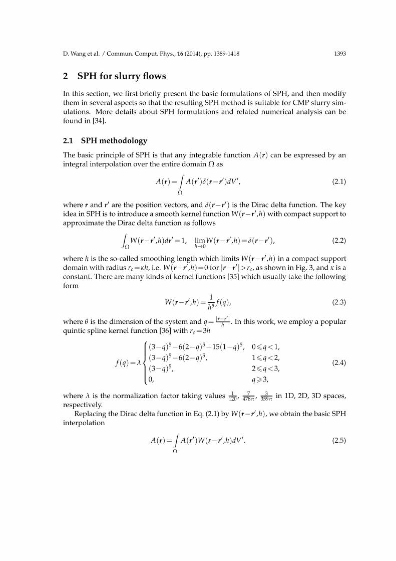
2 SPH for slurry flows

In this section, we first briefly present the basic formulations of SPH, and then modifythem in several aspects so that the resulting SPH method is suitable for CMP slurry sim-ulations. More details about SPH formulations and related numerical analysis can befound in [34].

2.1 SPH methodology

The basic principle of SPH is that any integrable function A(r) can be expressed by anintegral interpolation over the entire domain Ω as

A(r)=∫

Ω

A(r′)δ(r−r′)dV ′, (2.1)

where r and r′ are the position vectors, and δ(r−r′) is the Dirac delta function. The keyidea in SPH is to introduce a smooth kernel function W(r−r′,h) with compact support toapproximate the Dirac delta function as follows

∫

ΩW(r−r′ ,h)dr′=1, lim

h→0W(r−r′ ,h)=δ(r−r′), (2.2)

where h is the so-called smoothing length which limits W(r−r′ ,h) in a compact supportdomain with radius rc=κh, i.e. W(r−r′ ,h)=0 for |r−r′ |>rc, as shown in Fig. 3, and κ is aconstant. There are many kinds of kernel functions [35] which usually take the followingform

W(r−r′ ,h)=1

hθf (q), (2.3)

where θ is the dimension of the system and q= |r−r′|h . In this work, we employ a popular

quintic spline kernel function [36] with rc=3h

f (q)=λ

(3−q)5−6(2−q)5+15(1−q)5, 06q<1,

(3−q)5−6(2−q)5, 16q<2,

(3−q)5, 26q<3,

0, q>3,

(2.4)

where λ is the normalization factor taking values 1120 , 7

478π , 3359π in 1D, 2D, 3D spaces,

respectively.Replacing the Dirac delta function in Eq. (2.1) by W(r−r′ ,h), we obtain the basic SPH

interpolation

A(r)=∫

Ω

A(r′)W(r−r′ ,h)dV ′. (2.5)


W(r-r', h)

h

Figure 3: A sketch of the kernel function with compact support domain. The radius is rc =κh.

Using the summation over particles to approximate the integral, Eq. (2.5) becomes

Ai=∑j

AjWij

mj

ρj, (2.6)

where the particle i has mass mi, density ρi, position ri, Ai= A(ri), Wij =W(ri−rj,h) andthe summation is over all the particles but, in practice, it is only over near neighboursbecause W(r−r′ ,h) falls off rapidly with distance. Consequently, the derivative of A(r)with respect to r at ri can be given as [37]

∇Ai=−∑j

Aij∇iWij

mj

ρj, (2.7)

which is exact for a constant A, where Aij = Ai−Aj and ∇i denotes the gradient withrespect to the position of particle i. In the SPH community, the symmetric discretizationof ∇A(r) is often used to overcome the poor performance of (2.7) in momentum calcula-tion [38]. In this work, we adopted the particle-averaged spatial derivative proposed byHu et al. [39]

∇Ai=1

Vi∑

j

(V2i +V2

j )Aij∇iWij, (2.8)

where Aij= A(Ai,Aj) is an inter-particle average value and Vi=1/∑jWij. This discretiza-tion conserves linear and angular momentum exactly. It should be noted that there areother kinds of discretizations in the literature, see e.g. [37, 40], and we choose here thediscretization shown in (2.8) because it can be applied into multiphase flows [39] andeasily combined with the dummy particle boundary condition proposed in [32], both ofwhich are crucial in our CMP slurry simulations as discussed in Section 2.3.


2.2 Governing equations of SPH methods

The incompressible fluid can usually be approximated by a weakly compressible one [36,41], of which the governing equations are given by the compressible isothermal Navier-Stokes equations

dρ

dt=−ρ∇·v, (2.9)

ρdv

dt=−∇p+τ+ρ f , (2.10)

where ρ is the fluid density, v is the velocity, p, τ and f are the pressure, viscous force andbody force, respectively. Eq. (2.9) is the well-known continuity equation and Eq. (2.10) isthe momentum equation for the fluid. The pressure p in Eq. (2.10) is determined by theequation of state [42]

p=ρ0c2

γ

[(

ρ

ρ0

)γ

−1

]

, (2.11)

where ρ0 is the reference density which is often set equal to the initial density of fluid, cis the reference sound speed, and the exponent power γ is a constant. c is often set to 10times reference velocity, i.e. the Mach number of the compressible flow is less than 0.1.The stiffness of the equation of state can be adjusted with the parameter γ and for fluidsit is common to use γ=7. Assuming incompressibility of the fluid, the viscous force termin Eq. (2.10) can be simplified to

τ=η∇2v, (2.12)

where η is the dynamic viscosity. Then, Eq. (2.10) turns into

ρdv

dt=−∇p+η∇2v+ρ f . (2.13)

Based on Eqs. (2.6), (2.7), and (2.8), one can derive a SPH discretization for (2.9) and(2.13) as follows [32]

dρi

dt=ρi∑

j

vij ·∇iWij

mj

ρj, (2.14)

dvi

dt=

1

mi∑

j

(V2i +V2

j )

(

− pij∇iWij+ ηij

vij

rij

∂W

∂rij

)

+ fi, (2.15)

where rij=|rij|=|ri−rj| denotes the distance between particle i and j, ∂W∂rij

is the directional

derivative in the direction of eij =rij

rij(i.e. ∂W

∂rij=∇iWij ·eij), pij =

piρj+pjρi

ρi+ρjis the density-

weighted inter-particle averaged pressure, and ηij =2ηiηj

ηi+ηjis the inter-particle-averaged

viscosity.


2.3 No-slip and no-penetration boundary treatments

For astrophysical problems where fluid moves in the absence of boundaries, imposingboundary condition was not a matter of a big concern in SPH. However, when appliedto wall-bounded flows, SPH needs to address the important issue of enforcing suitableboundary conditions. Due to the absence of boundary terms in standard SPH formula-tions, the boundary conditions are usually imposed by adding boundary particles inter-acting with inner fluid particles.

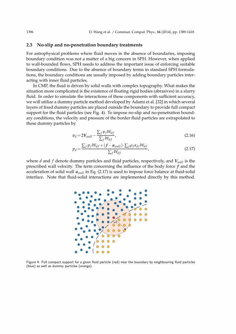
In CMP, the fluid is driven by solid walls with complex topography. What makes thesituation more complicated is the existence of floating rigid bodies (abrasives) in a slurryfluid. In order to simulate the interactions of these components with sufficient accuracy,we will utilize a dummy particle method developed by Adami et al. [32] in which severallayers of fixed dummy particles are placed outside the boundary to provide full compactsupport for the fluid particles (see Fig. 4). To impose no-slip and no-penetration bound-ary conditions, the velocity and pressure of the border fluid particles are extrapolated tothese dummy particles by

vd=2Vwall−∑ f v f Wd f

∑ f Wd f, (2.16)

pd =∑ f p f Wd f +( f−awall)·∑ f ρ f rd f Wd f

∑ f Wd f, (2.17)

where d and f denote dummy particles and fluid particles, respectively, and Vwall is theprescribed wall velocity. The term concerning the influence of the body force f and theacceleration of solid wall awall in Eq. (2.17) is used to impose force balance at fluid-solidinterface. Note that fluid-solid interactions are implemented directly by this method.

h

Figure 4: Full compact support for a given fluid particle (red) near the boundary by neighbouring fluid particles(blue) as well as dummy particles (orange).


Furthermore, since the dummy particles are fixed along the boundary, complex geome-tries can be handled easily. All these advantages make the dummy particle method thepreferable choice for our work.

2.4 Tensile and density instability treatments of an improved SPH

In the weakly compressible fluid approach, the standard SPH scheme suffers from twomain drawbacks. One is the well-known tensile instability caused by the clustering ofnegative-pressure fluid particles [43]. Various possible solutions have been proposed toeliminate such an instability. In this work, we employ a newly proposed method byAdami et al. [44], in which the movement of a particle is modified by an advection veloc-ity v as

dri

dt= vi, (2.18)

vi(t+∆t)=vi(t)+∆t

(

dvi

dt−

1

ρi∇pb

)

, (2.19)

dvi

dt=

dvi

dt+

1

mi∑

j

(V2i +V2

j )Ai+Aj

2·∇iWij, (2.20)

where pb is the background pressure and dvidt is the revised momentum equation by

adding an advection tensor ∇·A with A= ρv(v−v). It is shown in [44] that this tech-nique significantly reduces the clumping of particles.

The other factor affecting the SPH simulation results is the occurrence of spurious os-cillations in density and pressure fields. This phenomenon has not drawn much attentionin the SPH community as the focus of most investigations is on the velocity field whichcan be simulated nicely [45]. But when the problem involves fluid-solid interaction, thepressure field becomes a critical issue. To solve this problem, we use a kernel gradientcorrection method [46] in which ∇iWij in Eq. (2.14) is replaced by

∇iWij =Li∇iWij, (2.21)

where L is the correction matrix defined as

Li=(

−∑j

Vj∇iWij⊗rij

)−1. (2.22)

With the help of this kernel gradient correction technique, the oscillations in density andpressure field can be reduced significantly.

2.5 Slurry flows in SPH modelling

In CMP process, the slurry is transported and delivered to the pad-wafer interface by therelative movement of the pad and the wafer. A thin film of slurry flow, with thickness


around 20 µm [47], is formed by pressing the wafer against the pad. Moreover, becauseof the existence of the asperities on pad surface, the gap between asperity tips and thewafer can be much thinner. At such a microscopic scale together with a comparably highvelocity of the rough pad and the wafer, the slurry will behave quite differently frommacroscopic bulk fluid. For example, higher shear rate in the thin slurry film can beobserved at this scale [48].

In this work, the motion of slurry flow is calculated in the SPH framework. The fluidis driven either by the rough pad or by the plate wafer. On account of the Lagrangiancharacteristics, the fluid driven by the moving rough solid walls can easily be simulated.An important issue to be mentioned here is that the fluid is considered to be Newtonian,i.e. a constant viscosity for the fluid, despite of the fact that the fluid at this scale probablybehaves as non-Newtonian. However, we note that SPH has been shown to be capable ofhandling non-Newtonian flows as well, see e.g. [49], which would be considered in ourfuture work.

In the following, the modelling of two main physical processes in slurry flow will bediscussed.

2.5.1 Slurry-abrasive interactions

One of the most difficult problems in CMP slurry modellings is the motion of floatingabrasives (see Fig. 2), which makes the slurry a particulate fluid. Monaghan et al. [50]proposed a scheme describing the motion of the floating bodies by the solid wall bound-ary condition and Newton’s law of motion. Satisfactory results have been obtained bysimilar approach, see e.g. [51]. In this work, in order to achieve a unified treatment forboth solid boundaries and fluid-solid interactions, we extend the generalized dummyparticle method described in Section 2.3, which has not been used so far to handle thiskind of problem, to deal with floating bodies in slurry flows.

Let us consider one abrasive composed of many dummy particles in the SPH repre-sentation. The abrasive is regarded as rigid and surrounded by fluid particles, as illus-trated in Fig. 5. The force applied on the dummy particle d from all its neighbouring fluidparticles is

fd =md∑f

fd f , (2.23)

where f denotes the fluid particle. The motion of a rigid abrasive S can then be writtenas

MSdVS

dt= ∑

d∈S

fd, (2.24)

ISdΩS

dt= ∑

d∈S

(rd−rS)× fd, (2.25)

where M is the mass of the abrasive, I is the moment of inertia, V and Ω are the velocityand angular velocity, respectively, and rS is the centre of the rigid body. Finally, we have


d

Figure 5: An abrasive is formed by dummy particles (orange). The force exerted on a dummy particle d issummed from all fluid particles (blue) in its support domain.

the motion equation of the dummy particles belonging to the rigid abrasive S

drd

dt=VS+ΩS×(rd−rS). (2.26)

2.5.2 Solid-solid repulsive interactions

Since there is no interactions between dummy particles in SPH, when the rigid bodiesapproach each other or a floating body moves close to the solid wall, no repelling will oc-cur. This may lead to unphysical overlap of the solid materials. Therefore, it is necessaryto introduce a repulsive force to avoid this phenomenon. Here, we take the form of therepulsive force proposed by Glowinski et al. [52]

Fab =

0, |rab|>Ra+Rb+ζ,

cabǫ

( |rab|−Ra−Rb−ζζ

)2 rab

|rab|, |rab|≤Ra+Rb+ζ,

(2.27)

where cab is the force scale, ǫ is the stiffness factor, rab is the position vector pointingfrom the centre of rigid body a to b, R is the radius of the rigid body, ζ is the penaltydistance of the repulsive force. When the distance of two solid bodies is less than ζ, astrong repulsive force scaled by cab and ǫ will prevent them from penetrating each other.Meanwhile, if the floating abrasive approaches the solid wall, a mirror abrasive locatedoutside the wall will be used to provide the repulsion

Faw =

0, |raw |>2Ra+ζ,

cawǫ

( |raw|−2Ra−ζζ

)2 raw

|raw|, |raw |≤2Ra+ζ,

(2.28)

where raw is the position vector pointing from a to its mirror image.


2.6 Neighbour search algorithm

A large computational cost of SPH is associated with finding the neighbours of a givenparticle. Because of the compact support property of kernel function, only neighbourparticles in the support domain need to be considered in the interpolation of Ai, whichsignificantly reduces the computational costs of SPH. Thus, the development of an effi-cient neighbour search method is worthy of consideration.

A simple implementation of the neighbour search will traverse over all the particles.When the number of particles becomes very large, this method will be extremely time-costing. Therefore, many methods have been developed to reduce the search costs. Mostof these applications are based on the grid-link-list algorithm [53] and the hierarchicaltree structured algorithm [54]. Also, we have developed a competitive easy-to-parallelizeneighbour search method [33] based on the plane-sweep algorithm, and implemented itin this work. Satisfactory speed-up has been achieved with the help of this new algo-rithm, which makes large-scale simulations possible. More details can be found in [33].

2.7 Time integration

Considering the advection correction method in velocity field to overcome tensile insta-bility, a modified velocity-Verlet scheme [44] is used to perform the time integration

vn+ 12 =vn+

∆t

2·( dv

dt

)

n

, (2.29)

vn+ 12 =vn+ 1

2 +∆t

2f n

pb, (2.30)

rn+ 12 = rn+

∆t

2vn+ 1

2 , (2.31)

where fpb= 1

ρ∇pb is the background pressure.

Then, the density is updated by Eq. (2.14) using the half time-step velocity vn+1/2 andposition rn+1/2 as follows

ρn+1=ρn+∆t( dρ

dt

)n+ 12

. (2.32)

Meanwhile, the position of the next step is updated by

rn+1= rn+ 12 +

∆t

2vn+ 1

2 . (2.33)

It should be noted that the advection velocity v is only used to move the particles to theirnew positions but not included in the calculation of density.

Finally, using the updated density ρn+1 and position rn+1, the forces at step n+1 canbe calculated. And the velocity for new time step can be obtained as

vn+1=vn+ 12 +

∆t

2

( dv

dt

)

n+1

. (2.34)


If the advection correction for eliminating the tensile instability is not used here, i.e.ignoring the background pressure term f n

pbin Eq. (2.30), the above time integration re-

duces to the conventional velocity-Verlet method.

The time step is set to the minimum of the Courant-Friedrichs-Lewy criterion [55],the viscous criterion [36] and the force criterion [56], namely,

∆t≤min

(

0.25h

c, 0.25

h2

ν, 0.25

√

h

| f |

)

, (2.35)

where ν is the kinematic viscosity, f is the body force per mass on the particle.

In summary, the overall SPH algorithm for slurry flows with abrasives is given inAlgorithm 1.

3 Feature scale modelling of CMP

The SPH method for slurry flows with abrasives developed in the last section will beused for feature scale CMP modelling next. Before presenting numerical results, in orderto deal with feature scale CMP problems, several models of the CMP process will beestablished first.

3.1 Non-contact removal model

In the feature-scale CMP regime, there are two main models describing the mechanismof material removals. One is the contact model, where the pad directly contacts with thewafer. The abrasives in the slurry are indented into wafer surface and the materials on thewafer are scratched off the surface. This model is first introduced by Kaufman et al. [57]and later widely accepted in the CMP community, see e.g. [23]. However, it has beenquestioned recently and a new model based on the non-contact hypothesis (i.e. thereis no real contact between pad and wafer) was proposed [58, 59]. Many experimentalresults have supported this hypothesis [60, 61]. In the non-contact model, the surfaceof the wafer is weakened by chemical reactions from the slurry. Then, only the surfacemolecules of the material are removed and carried away by the strong shearing force ofthe slurry and abrasives. In the present work, to investigate the effect of slurry flow inthe entire domain, the pad and the wafer is completely separated by the slurry, i.e. thenon-contact model is adopted.

3.2 Pad asperities

A typical polish pad is a polyurethane foam with great many porous structures. About30-50% of the pad surface is covered by these porous structures with diameter 40-60 µm.Each pore is separated with wall structures (asperities) of width 10-50 µm [62]. From the


Algorithm 1 The skeleton of the SPH solver for slurry flows with abrasives.

Initialize and discretize the system into SPH particles.for each time step n=1,2,··· ,N do

for each fluid particle i do

Update vn+ 12 by Eq. (2.29) using ( dv

dt )n

Update vn+ 12 by Eq. (2.30) using background pressure f n

pb

Update rn+ 12 by Eq. (2.31) using vn+ 1

2

end forfor each rigid body S do

Update dVSdt and dΩS

dt by Eqs. (2.24) and (2.25) from dummy particles d∈S

Update the velocity and position of dummy particles at n+ 12 by Eq. (2.26)

end forDo neighbour searchingCorrect kernel gradient by Eqs. (2.21) and (2.22)

Calculate ( dρdt )

n+ 12

by Eq. (2.14) using vn+ 12 and rn+ 1

2 according to the neighbour listfor each fluid particle i do

Update ρn+1 by Eq. (2.32)

Update particle position rn+1 by Eq. (2.33) using vn+ 12


Update the position of dummy particles at n+1 by Eq. (2.26)end forDo neighbour searchExtrapolate pressure, velocity of fluid field to dummy particlesCorrect kernel gradient by Eq. (2.21) and (2.22)Calculate the forces in Eq. (2.15) at n+1 using ρn+1 and rn+1

for each fluid particle i doUpdate velocity vn+1 using forces at n+1 by Eq. (2.34)


Update dVSdt and dΩS

dt by Eqs. (2.24) and (2.25) from dummy particles d∈SUpdate the velocity of dummy particles at n+1 by Eq. (2.26)

end forUpdate ∆t by Eq. (2.35)

end for

profile view of the pad-wafer interface at feature scale, as illustrated in Fig. 2, the pad as-perity behaves like a brush sweeping along the surface of the wafer. The moving of theseasperities significantly changes the hydrodynamics of slurry flows, leading to the effec-tive removal of the materials. In this work, the pad surface is modelled by several layersof dummy particles which provide full compact support for the fluid particles near theboundary. These dummy particles do not only prevent fluid particles from penetratingthe boundary, but also act as solid walls propelling fluid particles into motion.


Generally, the pad is elastic and deforms under the pressure from the wafer carrier.The modelling of pad usually incorporates elastic mechanics and contact mechanics the-ory. Although the elastic dynamics can be simulated very well in the SPH framework,see e.g. [63], the present work as the first step assumes the pad to be rigid, i.e. no defor-mations of the pad occur during the simulation, and all the dummy particles forming thepad are fixed to their relative positions.

4 Numerical results

In this section, we first validate the proposed SPH method for simple flows with tra-ditional CFD solvers. Then, the CMP process with Gaussian shaped rough pads andwafers containing features are investigated by SPH. Finally, we calculate the removalrate of slurry with abrasives through SPH simulations.

4.1 Validation of the SPH solver

We will validate our SPH solver with traditional flow solvers in two cases.

4.1.1 Case 1 – shear flow in a rough-wall channel

In order to validate the model for a pad asperity, a SPH simulation of shear flow in a two-dimensional rough-boundary channel is conducted. As illustrated in Fig. 6, the channelconsists of a plate as the top wall and a sine-shaped boundary as the bottom wall. Thelength of the channel is L and the height H can be expressed by

H=H0+HA cos

(

2π

Lx

)

. (4.1)

The two walls are moving relatively to each other. As a result, the fluid is driven by thedrag from the moving wall. The system is similar to, but slightly different from the un-wrapped journal bearing model which often appears in thin film lubrication field [64].For the journal bearing model, the curvature and the side leakage of fluid film can usu-ally be neglected when L≫ H, thus the model can be reduced to a Reynold’s equation,of which the analytical solutions are available [64]. However, in our case, the reducedReynold’s equation is not longer valid for L is comparable with H and we do not haveanalytical solutions any more.

Here, we let one of the two walls move while keep the other stationary. Both themotion of the top wall and the bottom wall are simulated. Due to the roughness of thebottom wall, it is difficult to conduct the simulation by mesh-based methods. However,for SPH, on account of its mesh-free characteristics, the code for simulating the movementof the bottom wall is almost identical to that for the top wall.

We set L = 3×10−5 m, H0 = 1×10−5 m, HA = 5×10−6 m, the density of fluid ρ =1000 kg/m3, the dynamic viscosity η = 1×10−3 Pa·s. The moving wall has a horizontal


L

Vwall

H0

HA

Figure 6: A sketch of the channel with sine-shaped boundary.

velocity Vwall =1 m/s. We set the sound speed c=10Vwall to keep the Mach number lessthan 0.1. Periodic boundary conditions are implemented at the inlet and outlet of thechannel. The dummy particle method is used to mimic the no-penetration solid wall andthe no-slip boundary condition for the velocity and the Neumann boundary conditionfor the pressure are applied. The initial particle spacing ∆x is 1×10−7 m, i.e. 30000 fluidparticles are used.

We take the results calculated by the finite element method (provided by FLUENT, acommercial software) for the same system as the reference solutions. Fig. 7(a) comparesthe pressure on the top wall calculated by SPH (one simulation is moving the top wall,the other is moving the bottom wall) and FLUENT (only moving the top wall) at theinstant when the stationary state is reached. In Fig. 7(b), the results of the shear stress onthe top wall obtained by SPH and FLUENT are shown. The 2D plots of the pressure fieldin the entire channel for both SPH and FLUENT are shown in Fig. 8. From Figs. 7 and8, we observe that the two SPH simulations give almost identical results and the resultsfrom SPH and FLUENT reach a satisfactory agreement. Moreover, moving the curvedwall (the bottom wall in Fig. 6) causes much sharper change in the initial fluid field than

0 0.5 1 1.5 2 2.5 3

x 10−5

−250

−200

−150

−100

−50

0

50

100

150

200

250

X [m]

Pre

ssur

e [P

a]

SPH (top moving)SPH (bottom moving)FLUENT

(a) Pressure.

0 0.5 1 1.5 2 2.5 3

x 10−5

−220

−200

−180

−160

−140

−120

−100

−80

−60

−40

−20

X [m]

Wal

l She

ar S

tres

s [P

a]

SPH (top moving)SPH (bottom moving)FLUENT

(b) Shear stress.

Figure 7: Comparison of the forces on the top wall calculated by SPH (one simulation is moving the top wall,the other is moving the bottom wall) and the commercial software FLUENT.


X [m]

Y[m]

0 1E-05 2E-05 3E-050

5E-06

1E-05

1.5E-05Pressure

280

250

220

190

160

130

100

70

40

10

-20

-50

-80

-110

-140

-170

-200

-230

-260

-290

-320

-350

(a) SPH.

X [m]

Y[m]

0 5E-06 1E-05 1.5E-05 2E-05 2.5E-05 3E-050

5E-06

1E-05

1.5E-05Pressure

280

250

220

190

160

130

100

70

40

10

-20

-50

-80

-110

-140

-170

-200

-230

-260

-290

-320

-350

(b) FLUENT.

Figure 8: Comparison of the pressure field obtained by SPH (a) and FLUENT (b).

moving the flat wall (the top wall in Fig. 6), so that the channel flow is more difficult toreach stationary state in the former case. An initial damping [41] is often introduced tosolve such difficulty. In current simulations, we do not employ the initial damping, butstill get satisfactory results. Actually, the time reaching the stationary state with SPH is6×10−5 s (resp. 3×10−5 s) in the case of moving the curved (resp. flat) wall.

4.1.2 Case 2 – sedimentation of two cylinders in viscous fluid

To verify the model of fluid-solid interaction and solid-solid collision, we conducted asimulation of sedimentation of two cylinders in viscous flow. The two identical rigidcylinders are positioned along the central line of the vertical channel, as shown in Fig. 9(a).The system is initially at rest and the two cylinders will fall down due to gravity. The set-tling of the lower cylinder will generate a decrease in the pressure field behind, makingthe upper cylinder fall faster than the lower one. As a result, the upper cylinder willcatch up with the lower one. Then, the two cylinders will form a binary body system,which usually rotates to make the centre line perpendicular to the stream in the viscousflow. Finally, the two cylinders separate. This phenomenon is well known as “drafting,kissing and tumbling” (DKT) [65], and has been numerically simulated in [52,66–68] withdifferent numerical methods.

In this work, we adopt the same parameters in [52]. The channel width L=0.02 m, theheight H=0.06 m. The diameter of the cylinder is 0.0025 m. The bottom left corner of thechannel is set to be the origin, and the two cylinders are initially positioned at (0.01 m,0.045 m) and (0.01 m, 0.05 m), respectively. The density of the fluid (resp. cylinder) is1000 kg/m3 (resp. 1500 kg/m3). The dynamic viscosity of the fluid is 1×10−3 Pa·s. Thesystem is discretized into particles with initial spacing ∆x= 1×10−4 m, namely, 124836particles are used. To guarantee the accuracy of the weakly compressible flow approach,the sound speed c is set to be 10

√

gH with g being the gravitational acceleration. Eachcylinder is formed by 484 latticed dummy particles. The motion of the cylinder is deter-mined by the model of fluid-solid interaction discussed before in Section 2.5.1. The forcescale factors cab and caw are of the same value as g and ǫ=5×10−6. The penalty distanceζ in solid-solid collision shown in Eqs. (2.27) and (2.28) is 3∆x.


(a)

L

H

H1H2

(b)0 0.005 0.01 0.015 0.02

0

0.01

0.02

0.03

0.04

0.05

0.06

X [m]

Y [m

]

Leading cylinderTrailing cylinder

t=0.15sDrafting

t=0.2sKissing

t=0.3sTumbling

t=0s

Figure 9: Sedimentation of two cylinders in a vertical channel: (a) The sketch of the system at initial state; (b)The snapshots of cylinder settling simulated by SPH, where the process of drafting (t=0.15 s), kissing (t=0.2 s)and tumbling (t=0.3 s) is clearly shown.

Fig. 9(b) shows the trajectories of the two cylinders in the SPH simulation and theDKT process is clearly observed. In Figs. 10 and 11, we further compare the horizontalposition, the vertical position, the horizontal velocity and the vertical velocity calculatedwith SPH with those obtained by Glowinski et al. with a Lagrange-multiplier-based fic-titious domain method [52] and by Uhlmann with an immersed boundary method [68].It is shown there that the results from aforementioned two methods and SPH are in goodagreement until the “kissing” stage starts. After the collision of two cylinders, the fluidfield could be unstable and sensitive to the numerical methods adopted, as shown inFigs. 10 and 11. Such instability has been also reported before by Uhlmann [68], and ourresults are in more agreement with that by Uhlmann than by Glowinski et al. In a word,our SPH solver in Algorithm 1 can capture the physical moving trend of the two cylin-ders and thus is able to mimic the fluid-solid interactions and the solid-solid collisionsexisting in the CMP Slurry.

4.2 Flow with a Gaussian asperity and a flat wafer

In a previous work of our group [62], the effect of pad asperities on material removal inCMP was modelled and the importance of pad-wafer geometries was discussed in detail.However, the slurry flows were not included in that work. To further understand thegeometrical effect on slurry hydrodynamics, we conducted a series of simulations usinga moving wall with a Gaussian shape. As illustrated in Fig. 12(a), the channel consists of


0 0.05 0.1 0.15 0.2 0.25 0.30

0.002

0.004

0.006

0.008

0.01

0.012

0.014

0.016

0.018

0.02

Time [s]

X [m

]

SPHGlowinski et al. 2001Uhlmann 2005

(a) Horizontal position.

0 0.05 0.1 0.15 0.2 0.25 0.30

0.01

0.02

0.03

0.04

0.05

0.06

Time [s]

Y [m

]


(b) Vertical position.

Figure 10: Comparison of the position of the two cylinders calculated in this paper with SPH, by Glowinski etal. [52] and by Uhlmann [68].

0 0.05 0.1 0.15 0.2 0.25 0.3−0.02

0

0.02

0.04

0.06

0.08

0.1

Time [s]

Vx [m

/s]


(a) Horizontal velocity.

0 0.05 0.1 0.15 0.2 0.25 0.3−0.2

−0.18

−0.16

−0.14

−0.12

−0.1

−0.08

−0.06

−0.04

−0.02

0

Time [s]

Vy [m

/s]


(b) Vertical velocity.

Figure 11: Comparison of the velocity of the two cylinders calculated in this paper with SPH, by Glowinski etal. [52] and by Uhlmann [68].

a plate and a Gaussian-curve wall (asperity), of which the height is defined by

H=(Hmax−Hgap)e−

(x−x0)2

2σ2 , (4.2)

where x0 denotes the position of the peak and σ determines the width of the roughboundary. The curved wall is used to mimic the pad asperity and the plate representsthe wafer surface. The fluid is moved by the curved wall at a velocity Vwall in horizontaldirection, which is very similar to the CMP process.

The system is set in accordance with the genuine CMP materials. The fluid filmthickness is around 2×10−5 m [18, 47], and the width of asperity is from 1×10−6 m to1×10−5 m, and σ from 2×10−6 m to 1×10−5 m. The velocity of the moving boundary isVwall =1 m/s and the largest gap between the two boundaries is Hmax =2×10−5 m. Thefluid is set as water with ρ=1000 kg/m3 and η=1×10−3 Pa·s. The initial particle spacing∆x=2×10−7 m. The sound speed is set to be 10Vwall .


Hgap

Hmax

Vwall

(a) Flat wafer.

H

Hmax

V

(b) Arc-shaped feature.

H

Hmax

V

(c) Cavity.

H

Hmax

V

(d) Sine-shaped feature.

Figure 12: Sketches of the channel with a Gaussian-curve asperity on the bottom wall and several types oftypical features on the top wall.

The effects of σ and Hgap on the maximum fluid pressure along the horizontal liney=Hmax are shown in Fig. 13, from which we can see that the pressure increases almostlinearly with the increment of the width of the asperity (see Fig. 13(a) and e.g. the slope isabout 9.28 for Hgap=7×10−6 m), but grows exponentially when the gap becomes narrow(see Fig. 13(b) and e.g. the curve is e−3.636Hgap for σ = 6×10−6 m). Therefore, it can beconcluded that the height of the asperity plays a more important role in influencing thefluid pressure distribution.

1 2 3 4 5 6 7 8 9 100

100

200

300

400

500

600

700

800

σ [10−6m]

P [P

a]

Hgap

[10−6m]

119753

(a) Effect of asperity width σ.

2 3 4 5 6 7 8 9 10 11 120

100

200

300

400

500

600

700

800

900

Hgap

[10−6m]

P [P

a]

σ [10−6m]

2345678910

(b) Effect of asperity height Hgap.

Figure 13: Effect of the asperity geometry on the pressure.


4.3 Flow with a Gaussian asperity and a wafer with features

When the wafer surface is not flat, the pressure distribution will change by the featuresof the wafer. High pressure zone would occur in the feature area of the wafer and leadto a large material removal rate. Simulations on the effect of wafer features on the fluidhave been reported by Qin [69] using a finite element method. His results indicated thatthe removal of materials will start in the corner first and then happen on the bulk of thefeature. However, Qin only considered the planar pad surface and the flow was drivenby the motion of the flat pad. In our simulations, we investigate the effect of both padasperities and wafer features on the fluid. Particularly, three cases with different wafertopography are conducted below.

4.3.1 Case I – Arc-shaped feature on the wafer

As illustrated in Fig. 12(b), the channel consists of two rough solid boundaries. The topboundary mimics the wafer with an arc-shaped feature, while the bottom surface definedby Eq. (4.3) is used to simulate a rough pad

H=Hae−

(x−x0)2

2σ2 . (4.3)

Here, we set the channel length L = 8σ with σ = 5×10−6 m, the height of the asperityHa = 1.3×10−5 m, and the largest gap of the channel Hmax = 2×10−5 m. The radius ofthe arc feature on the top boundary is 5×10−6 m. The central angle of the arc is 2π/3 inradian, making the height of the feature 2.5×10−6 m.

To simulate the polishing process, we move the bottom wall horizontally and peri-odically at a constant speed of Vwall = 1 m/s. Thus the period T of the movement ofasperity is 4×10−5 s. The density of the fluid ρ=1000 kg/m3 and the dynamical viscosityη=1×10−3 Pa·s. The initial particle spacing ∆x=2×10−7 m and the sound speed is set to

2 2.4 2.8 3.2 3.6 4−200

−100

0

100

200

300

400

500

600

Time [10−4s]

Pre

ssur

e [P

a]

Figure 14: Evolution of the pressure at the sample point (2.3×10−6 m, 1.85×10−6 m) located at the featuresurface. The largest pressure occurs at about 0.7T.


0

1

2x 10

−5

Y [m

]

t0

0

1

2x 10

−5

Y [m

]

t0 + 0.2T

0

1

2x 10

−5

Y [m

]

t0 + 0.4T

0

1

2x 10

−5

Y [m

]

t0 + 0.6T

0 1 2 3 4

x 10−5

0

1

2x 10

−5

X [m]

Y [m

]

t0 + 0.8T

Pressure [Pa]

−500 0 500

(a) Arc-shaped feature.

0

1

2

x 10−5

Y [m

]

t0

0

1

2

x 10−5

Y [m

]

t0 + 0.2T

0

1

2

x 10−5

Y [m

]t0 + 0.4T

0

1

2

x 10−5

Y [m

]

t0 + 0.6T

0 1 2 3 4

x 10−5

0

1

2

x 10−5

X [m]

Y [m

]

t0 + 0.8T

Pressure [Pa]

−200 0 200 400

(b) Cavity on the wafer.

0

1

2

x 10−5

Y [m

]

t0

0

1

2

x 10−5

Y [m

]

t0 + 0.2T

0

1

2

x 10−5

Y [m

]

t0 + 0.4T

0

1

2

x 10−5

Y [m

]

t0 + 0.6T

0 1 2 3 4

x 10−5

0

1

2

x 10−5

X [m]

Y [m

]

t0 + 0.8T

Pressure [Pa]

−500 0 500

(c) Sine-shaped defect.

Figure 15: Evolution of the pressure field of flows with a Gaussian asperity and a wafer with different featuresat different time instants.

be 10Vwall . The evolution of the pressure field at different instants is shown in Fig. 15(a),from which we can observe that: (a) A high pressure zone (red) appears around the tip ofthe asperity; (b) When the asperity is getting close to the feature, the high-pressure zoneextends to the corner area of the feature. Finally, the pressure on the feature reaches itspeak value at about 0.7T (see Fig. 14).

It is widely accepted that the removal happens when the forces on the wafer surfacegrow over the bond-break threshold of surface molecules and the MRR is sensible to themagnitude and frequency of the stresses on the wafer [58,60,61]. From the results shownin Figs. 14 and 15, we could get a clear view of how the forces on the wafer accumu-lates. Meanwhile, the importance of pad asperity to the periodical force accumulation ismanifested in this study.

4.3.2 Case II – A cavity on the wafer

In Case II, a hollow on the wafer (see Fig. 12(c)) is used to mimic the dishing of metalor erosion of dielectric in CMP. The parameters used in this case are the same as Case Iexcept that the arc is turned upside down. Fig. 15(b) shows the evolution of pressure field


from t0 to t0+0.8T. Similar to Case I, a high pressure zone is formed around the cornerarea. This indicates that the removal will most probably happen near the corner, whichagrees with the experimental results reported by White et al. [70]. In an electron micro-scopic image, it is shown clearly that a large removal occurs on the edge of a cylindricalpolydimethylsiloxane post in a cylindrical well.

4.3.3 Case III – Sine-shaped feature on the wafer

The schematic of the Case III is plotted in Fig. 12(d). A sine-like defect is used in thiscase to mimic the topography of wafer surface due to the deposition of removed materialbehind the hollow. The deposing phenomenon is due to the abrasive-wafer collision andhas been reported in many microscopic simulations, see e.g. [25,71]. The amplitude of thesine-like defect is 2.5×10−6 m in accordance with the height of arc features in Cases I andII, while other parameters keep unchanged. In Fig. 15(c), as expected, a high-pressurezone is formed around the pile when the asperity is approaching. With the help of thehigh stresses, the pile of weakened molecules behind the hollow can easily be transportedaway by slurry flows.

The results of the above three cases give us a preliminary insight of how the asperity-driving flow acts on the removal of materials. Near the area where material removal onthe wafer most probably happens, a high-stress zone in the fluid field can be found. Thisphenomenon agrees well with the model in non-contact hypothesis, where the removaland advection of weakened materials are most conducted by the slurry flow. Since thesecritical behaviours of the slurry flow is influenced by the moving pad asperities, it canbe demonstrated that the pad asperity plays an fundamentally important role in CMPprocess.

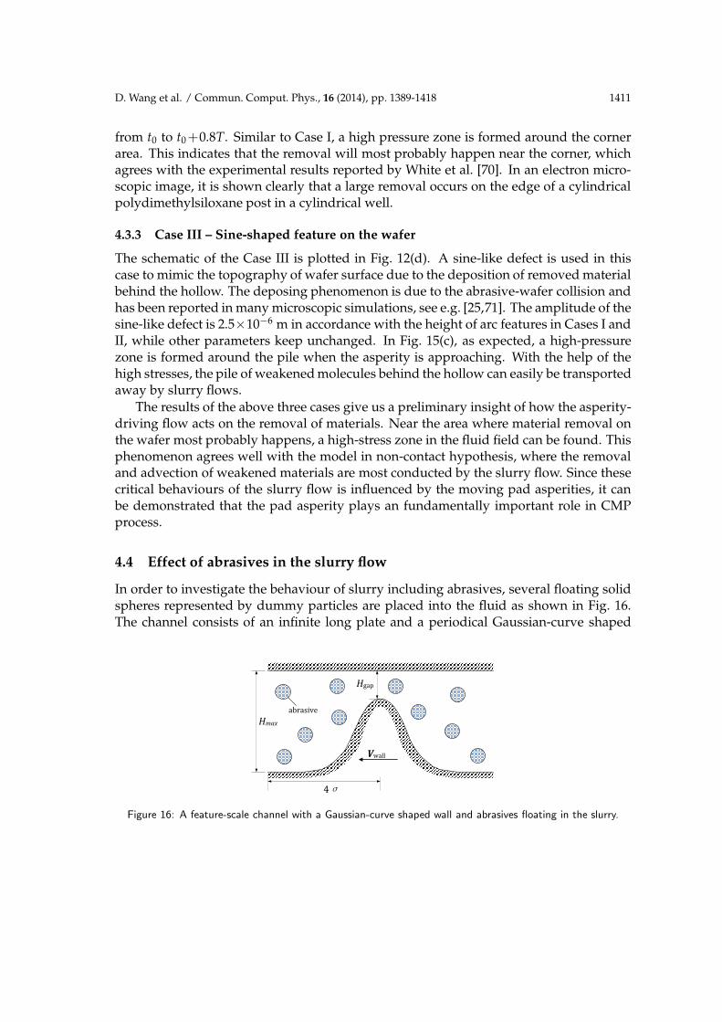
4.4 Effect of abrasives in the slurry flow

In order to investigate the behaviour of slurry including abrasives, several floating solidspheres represented by dummy particles are placed into the fluid as shown in Fig. 16.The channel consists of an infinite long plate and a periodical Gaussian-curve shaped

H

Hmax

V

Figure 16: A feature-scale channel with a Gaussian-curve shaped wall and abrasives floating in the slurry.


Table 1: The relation between the abrasive concentration and the number of abrasives.

# of abrasives 4 8 11 15 19 22 25 29

wt(%) 1.07 1.87 2.94 3.75 5.08 5.89 6.69 7.49

rough wall, and the fluid film thickness is determined by Eq. (4.2). In this simulation, weset H=2×10−5 m, σ=5×10−6 m, Vwall =1 m/s, ρ=1000 kg/m3, η=1×10−3 Pa·s. Theinitial SPH particle spacing is 1×10−7 m. The diameter of each cylinder is 1×10−6 m, i.e.80 dummy particles are used to form the sphere. The density of the abrasive is set to be2000 kg/m3. We performed a series of simulations with different abrasive concentrationwt% from 1.07% to 7.49% for which the numbers of abrasives are calculated by

n=wt%ρ f luidVf luid

(1−wt%)ρabrasiveVabrasive. (4.4)

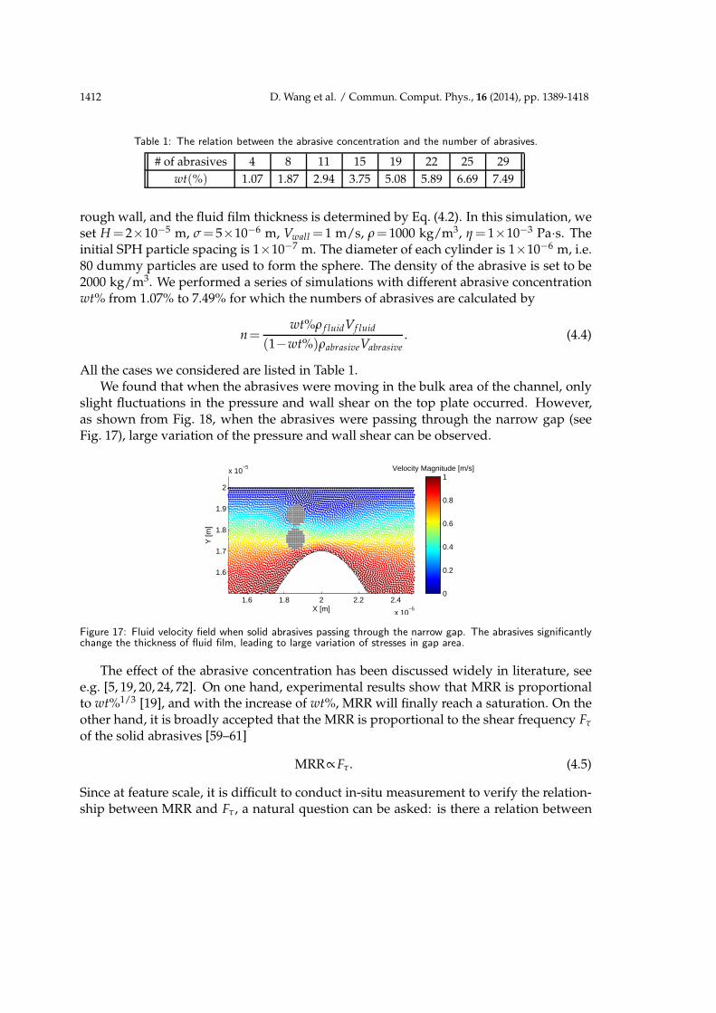
All the cases we considered are listed in Table 1.We found that when the abrasives were moving in the bulk area of the channel, only

slight fluctuations in the pressure and wall shear on the top plate occurred. However,as shown from Fig. 18, when the abrasives were passing through the narrow gap (seeFig. 17), large variation of the pressure and wall shear can be observed.

1.6 1.8 2 2.2 2.4

x 10−5

1.6

1.7

1.8

1.9

2

x 10−5

X [m]

Y [m

]

Velocity Magnitude [m/s]

0

0.2

0.4

0.6

0.8

1

Figure 17: Fluid velocity field when solid abrasives passing through the narrow gap. The abrasives significantlychange the thickness of fluid film, leading to large variation of stresses in gap area.

The effect of the abrasive concentration has been discussed widely in literature, seee.g. [5, 19, 20, 24, 72]. On one hand, experimental results show that MRR is proportionalto wt%1/3 [19], and with the increase of wt%, MRR will finally reach a saturation. On theother hand, it is broadly accepted that the MRR is proportional to the shear frequency Fτ

of the solid abrasives [59–61]

MRR∝ Fτ. (4.5)

Since at feature scale, it is difficult to conduct in-situ measurement to verify the relation-ship between MRR and Fτ , a natural question can be asked: is there a relation between


0 0.5 1 1.5 2 2.5 3 3.5 4

x 10−5

−500

0

500

1000

X [m]

Pre

ssur

e [P

a]

without abrasives

with abrasives (t = 6x10−5s)


(a) Pressure.

0 0.5 1 1.5 2 2.5 3 3.5 4

x 10−5

−400

−300

−200

−100

0

100

200

X [m]

Wal

l She

ar S

tres

s [P

a]

without abrasives



(b) Shear stress.

Figure 18: The forces on the top wall of abrasive-free case (red circle), abrasive-in-gap case (magenta *) andabrasive-beyond-gap case (blue +).

wt% and Fτ? or does Fτ ∝ (wt%)1/3 hold? We tried to answer this question with our SPHsimulations.

From Fig. 18(b), large shear stress can be found when the abrasives passing throughthe wafer-pad gap. Since the shearing force τ plays an important role in material remov-ing at feature scale [61], we assume that the material removal will most probably happenwhen the abrasive-leading high shear stress passes over a certain threshold τth. In thiswork, we set τth naturally to be the maximum shear stress on wafer surface when wt%=0(i.e. the abrasive-free case). With current settings, τth=288.5 Pa. If τ>τth, then τ is consid-ered as an active shear. Thus we could record the time tactive when the active shear occursduring a period of time ttotal for various wt%. In consequence, the frequency of the activeshear is measured by

Fτ =tactive

ttotal. (4.6)

Fig. 19 shows the relationship between the normalized abrasive concentration (by themaximum wt% = 7.49% in Table 1) and the above shear frequency. We observed therethat: (a) The shear frequency increases evidently as the number of the abrasives is in-creasing; (b) After a certain wt% (about 5%), Fτ reaches its saturation point and will notincrease thereafter; (c) Before the saturation, we may have the relation Fτ ∝ (wt%)1/3

holds. Therefore, our results are in good agreement with the aforementioned experimen-tal observation of the removal saturation in terms of abrasive concentration. Moreover,we confirmed numerically that Fτ ∝ (wt%)1/3 (which has not been done before either nu-merically or experimentally) holds before the saturation. It should be pointed out thatsince the establishment of threshold shear is based on the abrasive-free case, the analysisof active shear in this work can be applied to more complex and general situations in astraight way.


0 0.2 0.4 0.6 0.8 10.2

0.3

0.4

0.5

0.6

0.7

0.8

0.9

1

Normalized wt%

Act

ive

She

ar F

requ

ency

Wall Shear > 288.5 Pa

Saturation

(a)

0.5 0.55 0.6 0.65 0.7 0.75 0.8 0.85 0.90.2

0.3

0.4

0.5

0.6

0.7

0.8

0.9

1

Act

ive

She

ar F

requ

ency

(Normalized wt%)1/3

SPH dataFitting line

Fτ = C⋅(Normalized wt%)1/3+D

C = 1.52D = −0.4849

(b)

Figure 19: The shear frequency v.s. the normalized abrasive concentration (by the maximum wt%= 7.49% inTable 1). (a) Shear frequency as a function of normalized wt%. The grey dashed line denotes wt%=5% (i.e.

the normalized abrasive concentration is about 0.67). (b) Shear frequency as a function of (normalized wt%)1/3

before the saturation.

5 Conclusions

In this work, a systematic development of a SPH method is conducted, and the resultingSPH solver is suitable for the simulation of abrasive-filled slurry flow and rough padsand feature-scale wafers in a CMP process. The effects of rough pad, wafer defects, mov-ing solid boundaries, slurry-abrasive interactions and abrasive collisions are taken intoaccount by the developed SPH method.

Several recent improvements on SPH are integrated into the SPH method to yieldbetter accuracy of fluid field. The methods for simulating solid floating and solid-solidcollisions is coupled with SPH to simulate particulate slurry flow. Numerical validationsshow that SPH is able to capture the phenomena of the multi-physical aspects behindCMP.

The simulations of moving rough pad, geometry of several types of typical featureson the wafer shed some light on the mechanisms of material removal in CMP. A thoroughsimulation concerning the abrasive concentration is carried out. The results of shear fre-quency based on statistical hypothesis are in a satisfactory qualitative agreement with theexperimental data and demonstrate that SPH is a suitable method for studying complexCMP mechanisms.

This work, to some extent, can be further improved on several physical aspects. Thenon-Newtonian characteristics of slurry flow, the elastic properties of polishing pad, di-rect simulation of the interactions between the abrasives and the wafer are not taken intoconsideration in this paper. These issues together with the coupling of SPH and othercomputational methods, such as molecular dynamics for a deeper insight into the mech-anisms of chemical mechanical polishing, will be the subject of our research in the future.


Acknowledgments

D.W., C.Y. and X.Z. were partially supported by National Natural Science Foundation ofChina (Nos. 61125401, 61376040, 61228401, 61274032), the National Basic Research Pro-gram of China (No. 2011CB309701), the National Major Science and Technology Spe-cial Project of China (Nos. 2011ZX01035-001-001-003, 2014ZX02301002-002), ShanghaiScience and Technology Committee project (No. 13XD1401100) and the State Key Lab-oratory of ASIC and System (Fudan University) research project (No. 11MS013). S.S. waspartially supported by the National Natural Science Foundation of China (Nos. 11101011,91330110), the Specialized Research Fund for the Doctoral Program of Higher Education(No. 20110001120112) and the State Key Laboratory of ASIC and System (Fudan Univer-sity) open research project (No. 10KF015). W.C. was partially supported by the US ArmyOffice of Research (No. W911NF-11-1-0364), the National Science Foundation of USA(No. DMS-1315128) and the National Natural Science Foundation of China (No. 91330110).

References

[1] P. B. Zantye, A. Kumar, A. K. Sikder, Chemical mechanical planarization for microelectronicsapplications, Mat. Sci. Eng. R 45 (2004) 89–220.

[2] M. Bielmann, U. Mahajan, R. K. Singh, Effect of particle size during tungsten chemical me-chanical polishing, Electrochem. Solid State Lett. 2 (8) (1999) 401–403.

[3] G. B. Basim, J. J. Adler, U. Mahajan, R. K. Singh, B. M. Moudgil, Effect of particle size ofchemical mechanical polishing slurries for enhanced polishing with minimal defects, J. Elec-trochem. Soc. 147 (9) (2000) 3523–3528.

[4] C. Zhou, L. Shan, J. R. Hight, S. Danyluk, S. H. Ng, A. J. Paszkowskic, Influence of col-loidal abrasive size on material removal rate and surface finish in SiO2 chemical mechanicalpolishing, Tribol. Trans. 45 (2) (2002) 232–238.

[5] E. Matijevic, S. V. Babu, Colloid aspects of chemical-mechanical planarization, J. ColloidInterface Sci. 320 (2008) 219–237.

[6] F. W. Preston, The theory and design of plate glass polishing machines, J. Soc. Glass Technol.11 (1927) 214–257.

[7] S. R. Runnels, L. M. Eyman, Tribology analysis of chemical-mechanical polishing, J. Elec-trochem. Soc. 141 (6) (1994) 1698–1701.

[8] J. Tichy, J. A. Levert, L. Shan, S. Danyluk, Contact mechanics and lubrication hydrodynamicsof chemical mechanical polishing, J. Electrochem. Soc. 146 (4) (1999) 1523–1528.

[9] S. Sundararajan, D. G. Thakurta, D. W. Schwendeman, S. P. Murarka, W. N. Gill, Two-dimensional wafer-scale chemical mechanical planarization models based on lubricationtheory and mass transport, J. Electrochem. Soc. 146 (2) (1999) 761–766.

[10] S. R. Runnels, Freature-scale fluid-based erosion modeling for chemical-mechanical polish-ing, J. Electrochem. Soc. 141 (7) (1994) 1900–1904.

[11] C.-H. Yao, D. L. Feke, K. M. Robinson, S. Meikle, Contact mechanics and lubrication hydro-dynamics of chemical mechanical polishing, J. Electrochem. Soc. 147 (4) (2000) 1502–1512.

[12] D. Arbelaez, T. I. Zohdi, D. A. Dornfeld, Modeling and simulation of material removal withparticulate flows, Comput. Mech. 42 (5) (2008) 749–759.


[13] C. Zhou, L. Shan, J. R. Hight, S. H. Ng, S. Danyluk, Fluid pressure and its effects on chemicalmechanical polishing, Wear 253 (2002) 430–437.

[14] N. Mueller, C. Rogers, V. P. Manno, R. White, M. Moinpour, In situ investigation of slurryflow fields during CMP, J. Electrochem. Soc. 156 (12) (2009) H908–H912.

[15] D. Zhao, Y. He, X. Lu, In situ measurement of fluid pressure at the wafer-pad interfaceduring chemical mechanical polishing of 12-inch wafer, J. Electrochem. Soc. 159 (1) (2012)H22–H28.

[16] E. J. Terrell, C. F. Higgs III, Hydrodynamics of slurry flow in chemical mechanical polishing,J. Electrochem. Soc. 153 (6) (2006) K15–K22.

[17] S.-S. Park, C.-H. Cho, Y. Ahn, Hydrodynamic analysis of chemical mechanical polishingprocess, Tribol. Int. 33 (2000) 723–730.

[18] S. H. Ng, Measurement and Modeling of Fluid Pressures in Chemical Mechanical Polishing,Ph.D. thesis, Georgia Institute of Technology (2005).

[19] K. Cooper, J. Cooper, J. Groschopf, J. Flake, Y. Solomentsev, J. Farkas, Effects of particleconcentration on chemical mechanical planarization, Electrochem. Solid State Lett. 5 (12)(2002) G109–G112.

[20] D. Tamboli, G. Banerjee, M. Waddell, Novel interpretations of CMP removal rate depen-dencies on slurry particle size and concentration, Electrochem. Solid State Lett. 7 (10) (2004)F62–F65.

[21] Z. Zhang, W. Liu, Z. Song, Effect of abrasive particle concentration on preliminary chemicalmechanical polishing of glass substrate, Microelectron. Eng. 87 (2010) 2168–2172.

[22] E. Paul, A model of chemical mechanical polishing, J. Electrochem. Soc. 148 (6) (2001) G355–G358.

[23] Y.-R. Jeng, P.-Y. Huang, A material removal rate model considering interfacial micro-contactwear behaviour for chemical mechanical polishing, J. Tribol.-Trans. ASME 127 (2005) 190–197.

[24] Y. Wang, Y. Zhao, W. An, Z. Ni, J. Wang, Modeling effects of abrasive particle size and con-centration on material removal at molecular scale in chemical mechanical polishing, Appl.Surf. Sci. 257 (2010) 249–253.

[25] Y. Y. Ye, R. Biswas, J. R. Morris, A. Bastawros, A. Chandra, Molecular dynamics simulationof nanoscale machining of copper, Nanotechnology 14 (10) (2003) 390–396.

[26] E. Chagarov, J. B. Adams, Molecular dynamics simulations of mechanical deformation ofamorphous silicon dioxide during chemical-mechanical polishing, J. Appl. Phys. 94 (6)(2003) 3853–3861.

[27] P. M. Agrawal, L. M. Raff, S. Bukkapatnam, R. Komanduri, Molecular dynamics investiga-tions on polishing of a silicon wafer with a diamond abrasive, Appl. Phys. A-Mater. Sci.Process. 100 (1) (2010) 89–104.

[28] L. B. Lucy, A numerical approach to the testing of the fission hypothesis, Astron. J. 82 (12)(1977) 1013–1024.

[29] R. A. Gingold, J. J. Monaghan, Smoothed particle hydrodynamics: Theory and applicationto non-spherical stars, Mon. Not. Roy. Astron. Soc. 181 (1977) 375–389.

[30] J. J. Monaghan, Smoothed particle hydrodynamics and its diverse applications, Annu. Rev.Fluid Mech. 44 (1) (2012) 323–346.

[31] K. Takano, K. Yamada, N. Takezawa, T. Suzuki, T. Inamura, SPH-based flow simulationof polishing slurry including polished debris in CMP, J. Jpn. Soc. Precis. Eng. 73 (1) (2007)90–95, in Japanese.

[32] S. Adami, X. Y. Hu, N. A. Adams, A generalized wall boundary condition for smoothed


particle hydrodynamics, J. Comput. Phys. 231 (2012) 7057–7075.[33] D. Wang, Y. S. Zhou, S. H. Shao, Effcient implementation of smoothed particle hydrodynam-

ics (SPH) with plane sweep algorithm, preprint (2013).[34] G. R. Liu, M. B. Liu, Smoothed Particle Hydrodynamics: A Meshfree Particle Method, World

Scientific Publishing Co. Pte. Ltd., Singapore, 2003.[35] W. Dehnen, H. Aly, Improving convergence in smoothed particle hydrodynamics simula-

tions without pairing instability, Mon. Not. Roy. Astron. Soc. 425 (2) (2012) 1068–1082.[36] J. P. Morris, P. J. Fox, Y. Zhu, Modeling low Reynolds number incompressible flows using

SPH, J. Comput. Phys. 136 (1997) 214–226.[37] J. J. Monaghan, Smoothed particle hydrodynamics, Rep. Prog. Phys. 68 (8) (2005) 1703–1759.[38] D. J. Price, Smoothed particle hydrodynamics and magnetohydrodynamics, J. Comput.

Phys. 231 (2012) 759–794.[39] X. Y. Hu, N. A. Adams, A multi-phase SPH method for macroscopic and mesoscopic flows,

J. Comput. Phys. 213 (2006) 844–861.[40] S. Marrone, M. Antuono, A. Colagrossi, G. Colicchio, D. Le Touze, G. Grazianni, δ-SPH

model for simulating violent impact flows, Comput. Methods Appl. Mech. Engrg. 200 (2011)1526–1542.

[41] J. J. Monaghan, Simulating free surface flows with SPH, J. Comput. Phys. 110 (1994) 399–406.[42] G. K. Batchelor, An Introduction to Fluid Dynamics, Cambridge University Press, Cam-

bridge, 1967.[43] J. J. Monaghan, SPH without a tensile instability, J. Comput. Phys. 159 (2) (2000) 290–311.[44] S. Adami, X. Y. Hu, N. A. Adams, A transport-velocity formulation for smoothed particle

hydrodynamics, J. Comput. Phys. 241 (2013) 292–307.[45] D. Molteni, A. Colagrossi, A simple procedure to improve the pressure evaluation in hydro-

dynamic context using the SPH, Comput. Phys. Commun. 180 (6) (2009) 861–872.[46] J. Bonet, T.-S. Lok, Variational and momentum preservation aspects of smooth particle hy-

drodynamic formulations, Comput. Methods Appl. Mech. Engrg. 180 (1999) 97–115.[47] J. Lu, C. Rogers, V. P. Manno, A. Philipossian, S. Anjur, M. Moinpour, Measurements of

slurry film thickness and wafer drag during CMP, J. Electrochem. Soc. 151 (4) (2004) G241–G247.

[48] W. Lortz, F. Menzel, R. Brandes, F. Klaessig, T. Knothe, T. Shibasaki, News from the M inCMP-viscosity of CMP slurries, a constant?, MRS Proc. 767 (2003) 47–56.

[49] X.-J. Fan, R. I. Tanner, R. Zheng, Smoothed particle hydrodynamics simulation of non-Newtonian moulding flow, J. Non-Newton. Fluid Mech. 165 (2010) 219–226.

[50] J. J. Monaghan, A. Kos, N. Issa, Fluid motion generated by impact, J. Waterw. Port Coast.Ocean Eng.-ASCE 129 (6) (2003) 250–260.

[51] B. Bouscasse, A. Colagrossi, S. Marrone, M. Antuono, Nonlinear water wave interactionwith floating bodies in SPH, J. Fluids Struct. 42 (2013) 112–129.

[52] R. Glowinski, T. W. Pan, T. I. Hesla, D. D. Joseph, J. Periaux, A fictitious domain approachto the direct numerical simulation of incompressible viscous flow past moving rigid bodies:application to particulate flow, J. Comput. Phys. 169 (2001) 363–426.

[53] J. J. Monaghan, Particle methods for hydrodynamics, Comput. Phys. Rep. 3 (2) (1985) 71–124.

[54] L. Hernquist, N. Katz, TreeSPH: A unification of SPH with the hierarchical tree method,Astrophys. J. Suppl. Ser. 70 (1989) 419–446.

[55] R. Courant, K. Friedrichs, H. Lewy, On the partial difference equations of mathematicalphysics, IBM J. Res. Dev. 11 (2) (1967) 215–234.


[56] J. J. Monaghan, Smoothed particle hydrodynamics, Annu. Rev. Astron. Astrophys. 30 (1992)543–574.

[57] F. B. Kaufman, D. B. Thompson, R. E. Broadie, M. A. Jaso, W. L. Guthrie, D. J. Pearson, M. B.Small, Chemical-mechanical polishing for fabricating patterned W metal features as chipinterconnects, J. Electrochem. Soc. 138 (11) (1991) 3460–3465.

[58] Y. Zhao, L. Chang, S. H. Kim, A mathematical model for chemical-mechanical polishingbased on formation and removal of weakly bonded molecular species, Wear 254 (2003) 332–339.

[59] L. Chang, On the CMP material removal at the molecular scale, J. Tribol.-Trans. ASME 129 (2)(2007) 436–437.

[60] H. Hocheng, H. Y. Tsai, Y. T. Su, Modeling and experimental analysis of the material removalrate in the chemical mechanical planarization of dielectric films and bare silicon wafers, J.Electrochem. Soc. 148 (10) (2001) G581–G586.

[61] J. Xin, W. Cai, J. A. Tichy, A fundamental model proposed for material removal in chemical-mechanical polishing, Wear 268 (2010) 837–844.

[62] C. Feng, C. Yan, J. Tao, X. Zeng, W. Cai, A contact-mechanics-based model for general roughpads in chemical mechanical polishing processes, J. Electrochem. Soc. 156 (7) (2009) H601–H611.

[63] C. Antoci, M. Gallati, S. Sibilla, Numerical simulation of fluid-structure interaction by SPH,Comput. Struct. 85 (2007) 879–890.

[64] B. J. Hamrock, S. R. Schmid, B. O. Jacobson, Fundamentals of Fluid Film Lubrication, 2ndEdition, Marcel Dekker, Inc., New York, USA, 2004.

[65] A. F. Fortes, D. D. Joseph, T. S. Lundgren, Nonlinear mechanics of fluidization of beds ofspherical particles, J. Fluid Mech. 177 (1987) 467–483.

[66] H. H. Hu, D. D. Joseph, M. J. Crochet, Direct simulation of fluid particle motions, Theor.Comput. Fluid Dyn. 3 (1992) 285–306.

[67] Z.-G. Feng, E. E. Michaelides, The immersed boundary-lattice Boltzmann method for solv-ing fluid-particles interaction problems, J. Comput. Phys. 195 (2004) 602–628.

[68] M. Uhlmann, An immersed boundary method with direct forcing for the simulation of par-ticulate flows, J. Comput. Phys. 209 (2005) 448–476.

[69] K. Qin, Multi-scale Modeling of the Slurry Flow and the Material Removal in ChemicalMechanical Polishing, Ph.D. thesis, The University of Florida (2003).

[70] R. D. White, A. J. Mueller, M. Shin, D. Gauthier, V. P. Manno, C. B. Rogers, Measurementof microscale shear forces during chemical mechanical planarization, J. Electrochem. Soc.158 (10) (2011) H1041–H1051.

[71] F. Ilie, Models of nanoparticles movement, collision, and friction in chemical mechanicalpolishing (CMP), J. Nanopart. Res. 14 (3) (2012) 752.

[72] R. K. Singh, S.-M. Lee, K.-S. Choi, G. Bahar Basim, W. Choi, Z. Chen, B. M. Moudgil, Funda-mentals of slurry design for CMP of metal and dielectric materials, MRS Bull. 27 (10) (2002)752–760.

Documents

Communications in Computational Physics