Communications in Statistics - Theory and Methods A ... · Straight lines are managed through their polar descriptors D , instead of the usual “slope, y-intercept” mb descriptors

PLEASE SCROLL DOWN FOR ARTICLE

This article was downloaded by: [Vazquez, Manuel]On: 2 December 2010Access details: Access Details: [subscription number 930484816]Publisher Taylor & FrancisInforma Ltd Registered in England and Wales Registered Number: 1072954 Registered office: Mortimer House, 37-41 Mortimer Street, London W1T 3JH, UK

Communications in Statistics - Theory and MethodsPublication details, including instructions for authors and subscription information:http://www.informaworld.com/smpp/title~content=t713597238

A Generalized Regression Methodology for Bivariate Heteroscedastic DataAntonio Fernándeza; Manuel Vázquezab

a Electronica Fisica, EUITT-UPM, Madrid, Spain b IES, UPM, Madrid, Spain

Online publication date: 02 December 2010

To cite this Article Fernández, Antonio and Vázquez, Manuel(2011) 'A Generalized Regression Methodology for BivariateHeteroscedastic Data', Communications in Statistics - Theory and Methods, 40: 4, 598 — 621To link to this Article: DOI: 10.1080/03610920903444011URL: http://dx.doi.org/10.1080/03610920903444011

Full terms and conditions of use: http://www.informaworld.com/terms-and-conditions-of-access.pdf

This article may be used for research, teaching and private study purposes. Any substantial orsystematic reproduction, re-distribution, re-selling, loan or sub-licensing, systematic supply ordistribution in any form to anyone is expressly forbidden.

The publisher does not give any warranty express or implied or make any representation that the contentswill be complete or accurate or up to date. The accuracy of any instructions, formulae and drug dosesshould be independently verified with primary sources. The publisher shall not be liable for any loss,actions, claims, proceedings, demand or costs or damages whatsoever or howsoever caused arising directlyor indirectly in connection with or arising out of the use of this material.

http://www.informaworld.com/smpp/title~content=t713597238

http://dx.doi.org/10.1080/03610920903444011

http://www.informaworld.com/terms-and-conditions-of-access.pdf

Communications in Statistics—Theory and Methods, 40: 598–621, 2011Copyright © Taylor & Francis Group, LLCISSN: 0361-0926 print/1532-415X onlineDOI: 10.1080/03610920903444011

AGeneralized RegressionMethodologyfor Bivariate Heteroscedastic Data

ANTONIO FERNÁNDEZ1 AND MANUEL VÁZQUEZ1�2

1Electronica Fisica, EUITT-UPM, Madrid, Spain2IES, UPM, Madrid, Spain

We present a methodology for reducing a straight line fitting regression problemto a Least Squares minimization one. This is accomplished through the definitionof a measure on the data space that takes into account directional dependences oferrors, and the use of polar descriptors for straight lines. This strategy improves therobustness by avoiding singularities and non-describable lines.

The methodology is powerful enough to deal with non-normal bivariateheteroscedastic data error models, but can also supersede classical regressionmethods by making some particular assumptions. An implementation of themethodology for the normal bivariate case is developed and evaluated.

Keywords Errors in both axes; Heteroscedastic data; Linear regression.

Mathematics Subject Classification 62J02.

1. Introduction

Fitting data to straight line models (Rawlings et al., 1998) is one of the mostfrequently applied statistical procedures. It is widely used in the calibration processin analytical chemistry, in the accelerated lifetime models (González et al., 2009;Vázquez et al., 2007; Yu et al., 2008), and in many other applications where it isrequired to infer linear trends from a set of experimental data.

Least Squares (LS) techniques (Sayago et al., 2004) for estimating regressionsare normally preferred against Bayesian methods because they are easier to interpretand less computationally expensive

The complexity and power of LS methods depends on the error data model. Thesimplest LS methods, Ordinary Least Squares (OLS) or Weighted Least-Squares(WLS) (Asuero and González, 2007; Mandel and McCrackin, 1988), that considernon null error variance only in the response variable (Y-axis), are analyticallyresoluble. However, these methods are of limited scope because they assume thatthe explanatory variable (X-axis) is free of error.

Received June 17, 2009; Accepted October 27, 2009Address correspondence to Manuel Vázquez, Electronica Fisica, Carretera de Valencia

km. 7, Madrid 28031, Spain; E-mail: [email protected]

598

Downloaded By: [Vazquez, Manuel] At: 10:08 2 December 2010

Generalized Regression for Heteroscedastic Data 599

Other LS methods that take into account errors on any direction as TotalLeast Squares (TLS) (Markovsky and Van Huffel, 2007), or Bivariate Least Squares(BLS) that is also called Generalized Least Squares (GLS) (Cheng and Riu, 2006),have been also proposed. TLS pursue the minimization of the Euclidean Distancebetween straight line and data. BLS weights Y-axis errors with factors that takeinto account variances of data on both axes. BLS has no analytical solution forheteroscedastic data and must therefore be solved by means of numeric algorithms(Martínez et al., 1999).

However, all the above methods only deal with numerical variances, so they arenot able to take advantage of more detailed information embedded in the functionalknowledge of the data statistics model.

Moreover, they describe straight lines by means of the usual “slope, y-intercept”�m� b� descriptors; therefore, they have a singularity-ambiguity problem in thedescription of lines that are parallel to Y-axis. So, when they are applied to caseswhose solution is close to such lines, the results can be affected by severe andunpredictable inaccuracy.

In this article, we present a methodology that goes around these drawbacks,and makes it possible to deal, from a unified perspective, with the most complexsituations where the data uncertainty is modelled by arbitrary statistics. We havedeveloped this methodology, contributing innovations in three stages:

• The approach. The Target Radial Deviation Normalized Distance (TRDND)concept, which will be explained in Sec. 2.3, is the fundamental tool that willmake it possible to reduce a regression problem statistically formulated to theminimization of a cost function.This approach has an essential advantage: it is insensitive to the particularselection of axes on which the data are given. This is a consequence of thefact that TRDND only depends on the statistical data error model and noton the projection of the variances along the particular axes we are workingwith. In some sense, TRDND let us to introduce in the data space a measurethat comes directly from the statistical definition of each datum.Moreover, TRDND allows an intuitive conceptual understanding and ispowerful enough to be easily generalized to higher dimensions, to deal withnon normal errors, and to incorporate information about cross-correlationbetween the coordinates of each datum.

• The formulation. Straight lines are managed through their polar descriptors�D��, instead of the usual “slope, y-intercept” �m� b� descriptors as will beexplained in Sec. 2.1. This allows us, to be able to describe straight lines ina unified way (even if they are parallel to axes), and to increase the methodrobustness by avoiding singularities.

• The resolution. As the case of bivariate normal statistics data model isespecially useful, a detailed algorithm for this case has been developed. Theapplication of the two former steps to this statistic leads to a system of twohigh-degree polynomial equations that has not algebraic treatment. So aniterative method, PDIM (Polar Descriptors Iterative Method), for solving itwill be presented in Sec. 4. PDIM offers a good trade-off between robustnessand computation time, even when it has to process large amounts of data.

The proposed methodology has an interesting feature: when it is customizedfor normal data statistics, the classical methods mentioned above (OLS, WLS, TLS,


600 Fernández and Vázquez

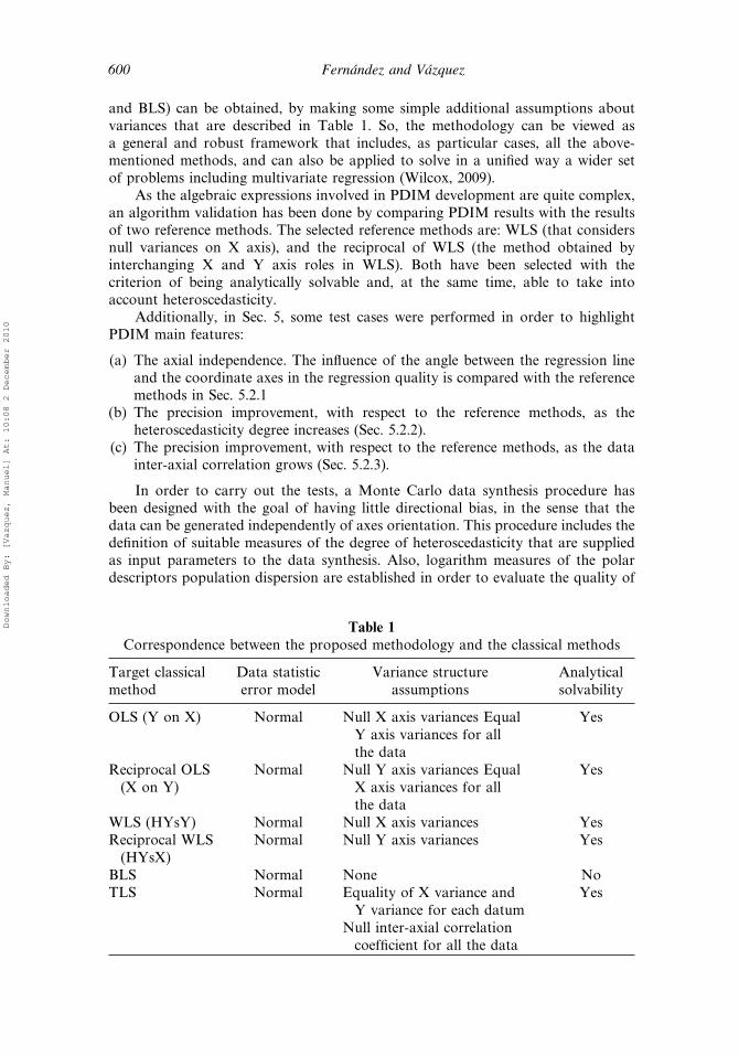
and BLS) can be obtained, by making some simple additional assumptions aboutvariances that are described in Table 1. So, the methodology can be viewed asa general and robust framework that includes, as particular cases, all the above-mentioned methods, and can also be applied to solve in a unified way a wider setof problems including multivariate regression (Wilcox, 2009).

As the algebraic expressions involved in PDIM development are quite complex,an algorithm validation has been done by comparing PDIM results with the resultsof two reference methods. The selected reference methods are: WLS (that considersnull variances on X axis), and the reciprocal of WLS (the method obtained byinterchanging X and Y axis roles in WLS). Both have been selected with thecriterion of being analytically solvable and, at the same time, able to take intoaccount heteroscedasticity.

Additionally, in Sec. 5, some test cases were performed in order to highlightPDIM main features:

(a) The axial independence. The influence of the angle between the regression lineand the coordinate axes in the regression quality is compared with the referencemethods in Sec. 5.2.1

(b) The precision improvement, with respect to the reference methods, as theheteroscedasticity degree increases (Sec. 5.2.2).

(c) The precision improvement, with respect to the reference methods, as the datainter-axial correlation grows (Sec. 5.2.3).

In order to carry out the tests, a Monte Carlo data synthesis procedure hasbeen designed with the goal of having little directional bias, in the sense that thedata can be generated independently of axes orientation. This procedure includes thedefinition of suitable measures of the degree of heteroscedasticity that are suppliedas input parameters to the data synthesis. Also, logarithm measures of the polardescriptors population dispersion are established in order to evaluate the quality of

Table 1Correspondence between the proposed methodology and the classical methods

Target classicalmethod

Data statisticerror model

Variance structureassumptions

Analyticalsolvability

OLS (Y on X) Normal Null X axis variances EqualY axis variances for allthe data

Yes

Reciprocal OLS(X on Y)

Normal Null Y axis variances EqualX axis variances for allthe data

Yes

WLS (HYsY) Normal Null X axis variances YesReciprocal WLS(HYsX)

Normal Null Y axis variances Yes

BLS Normal None NoTLS Normal Equality of X variance and

Y variance for each datumNull inter-axial correlationcoefficient for all the data

Yes



results. This scheme is described with detail in Sec. 5, so the methodology behaviorcan be evaluated and contrasted under any data profile.

2. Terminology and Tools

A first assumption that is commonly made in regression problems is the statisticalindependence of any datum with respect to the others. Although this is not everrigorously true in all situations, it allows each datum to be considered as anindividual entity that can be modeled by a single probability function. When thisassumption is satisfied, we will say that each datum is an uncertain point in the dataspace and the data set constitutes a cloud of uncertain points. An uncertain pointcan be fully defined given its measured values �xi� yi� on an (X, Y) axis referenceframe, and the error probability density function: f�i��xi� �yi�, that is a function thatdepends only on error components �xi� �yi along the (X, Y) axes. So the true pointvalue �xi� yi� can be obtained by means of (1):

xi ≡ xi − �xi(1)

yi ≡ yi − �yi

Once f�i��xi� �yi� is known, it is obvious to evaluate fi�xi� yi�, the ith datumprobability density function, by means of fi�xi� yi� = f�i�xi − xi� yi − yi�.

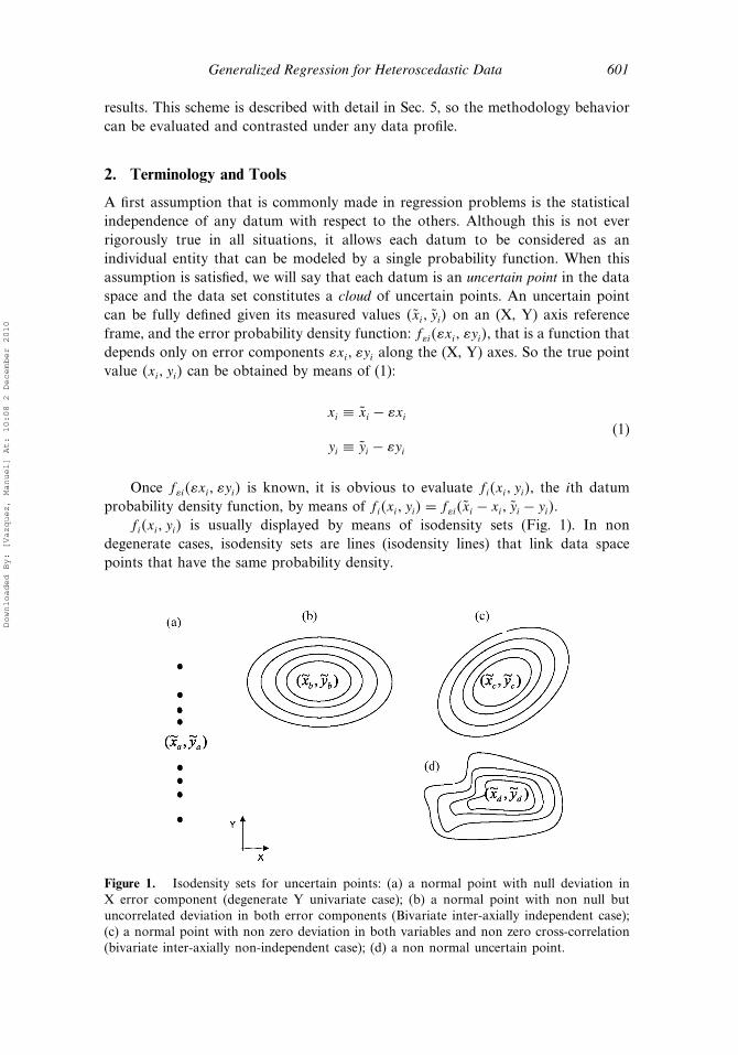
fi�xi� yi� is usually displayed by means of isodensity sets (Fig. 1). In nondegenerate cases, isodensity sets are lines (isodensity lines) that link data spacepoints that have the same probability density.

Figure 1. Isodensity sets for uncertain points: (a) a normal point with null deviation inX error component (degenerate Y univariate case); (b) a normal point with non null butuncorrelated deviation in both error components (Bivariate inter-axially independent case);(c) a normal point with non zero deviation in both variables and non zero cross-correlation(bivariate inter-axially non-independent case); (d) a non normal uncertain point.



We will say that an uncertain point is normal if the pair �xi� �yi follow a zeromean normal bivariate statistic (2):

f�i��xi� �yi� =1

2��xi�yi

√1− (

�xyi

)2× exp

[−12

1

1− (�xyi

)2(�x2i�2xi

+ �y2i�2yi

− 2�xyi

�xi�yi

�xi�yi

)] (2)

In (2), �xi� �yi are the marginal deviations of the two error components alongaxes, and �xyi is the inter-axial correlation coefficient. Once given these threeparameters, the inter-axial cross-covariance �2

xyi can be calculated as �xyi = �xyi�xi�yi.If the error components are independent, both �xyi and �xyi will be zero.

We will say that a cloud is a normal cloud when all its uncertain points arenormal, so a normal cloud can be completely described by a data structure that hasfive numeric descriptors �xi� �yi� �xyi� xi� yi� for each of its uncertain points.

Isodensity lines for normal points are the locus where the probability densityfunction (2) is constant. So, as a function of the error coordinates ��xi� �yi�,isodensity lines will have equations as (3):

�x2i�2xi

+ �y2i�2yi

− 2�xyi

�xi�yi

�2xi�2yi

= K2� (3)

where K is a parameter that labels each isodensity line. By (3), it is clear thatisodensity sets of normal uncertain points are ellipses centered on the origin in theerror space (or ellipses centered on the measurement �xi� yi� in the data space).

2.1. Straight Line Polar Descriptors

Using usual “slope, y-intercept” descriptors �m� b� or “counter-slope, x-intercept”�n� a� to represent straight lines in the forms (4) or (5) leads to unsafe computationssince both parameters can be unbounded:

y = mx + b (4)

x = ny + a (5)

That occurs because as lines get more strongly sloped, the magnitudes of m andb grow towards infinity. So for computational purposes, it is better to define straightlines with their polar descriptors �D��. Polar descriptors of a straight line shouldnot be confused with the polar coordinates of a point.

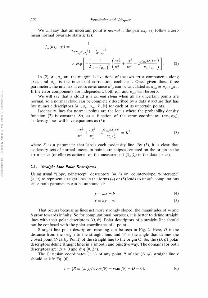
Straight line polar descriptors meaning can be seen in Fig. 2. Here, D is thedistance from the origin to the straight line, and � is the angle that defines theclosest point (Nearby Point) of the straight line to the origin O. So, the �D�� polardescriptors define straight lines in a smooth and bijective way. The domains for bothdescriptors are: D ≥ 0 and � ∈ 0� 2��.

The Cartesian coordinates �x� y� of any point R of the �D�� straight line rshould satisfy Eq. (6):

r = R ≡ �x� y�/x cos��+ y sin��−D = 0� (6)



Figure 2. Straight line polar descriptors.

So, its coordinates can be calculated, once given the deflection angle �R of pointR as (7):

R ≡{x = D cos��−D sin�� tan��R�

y = D sin��+D cos�� tan��R�(7)

Or as a function of the alternative parameter �R = D tan�R that describes apoint R by its signed distance �R from the nearby point (8):

x = D cos�− �R sin�

y = D sin�+ �R cos�(8)

2.2. Radial Deviation

Radial deviation is a measure that quantifies the error an uncertain point has alonga particular direction. The radial deviation can be calculated as a function of theangle � that defines a given direction. Expressing the error components of theuncertain point i in polar coordinates we have (9):

�xi = r cos �

�yi = r sin �(9)

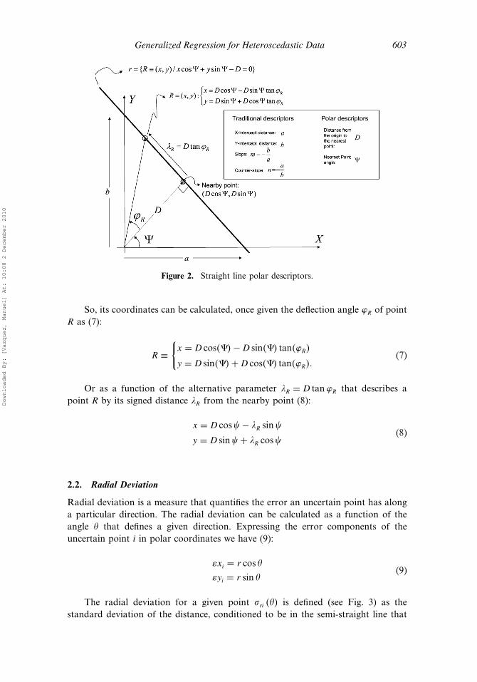
The radial deviation for a given point �ri �� is defined (see Fig. 3) as thestandard deviation of the distance, conditioned to be in the semi-straight line that



Figure 3. Experimental points are modeled by uncertain points centered in the measuredvalues. The Radial Deviation contour is defined by the Radial Deviation of the error fordifferent � values.

starts in �xi� yi� and forms an angle � with the X-axis, and can be calculated as (10):

�2ri �� =

∫ �0 r2f�i�r cos �� r sin ��dr∫ �0 f�i�r cos �� r sin ��dr

� (10)

where f�i�r cos �� r sin �� is the error probability density function in a specificdirection defined by the angle �. In Fig. 3 , the locus defined by the radial deviationfor different � values has been represented.

Radial deviation, �ri ��, should not be mistaken with �Di ��: the marginaldirectional deviation (Duda et al., 1997), that can be calculated by means of (11):

�2Di �� = 2

∫ �

0

∫ �

−�u2f�i�u cos �− v sin �� u sin �+ v cos ��dv du (11)

2.2.1. Radial Deviation of a Normal Point. It can be easily demonstrated, bytransforming (2) by (9), that the error associated with a normal point along aparticular radius (defined by the angle ��, follows a normal distribution. Moreover,the radial deviations contour �ri�� (that is the locus described by a vector thatforms an angle � with the X-axis, and whose modulus is precisely �ri��, draws anellipse that matches with an isodensity line whose equation is (12):

�2ri�� =

�2xi�

2yi�1− �2

xyi�

�2xi sin

2 �− 2�xyi�xi�yi sin � cos �+ �2yi cos2 �

(12)

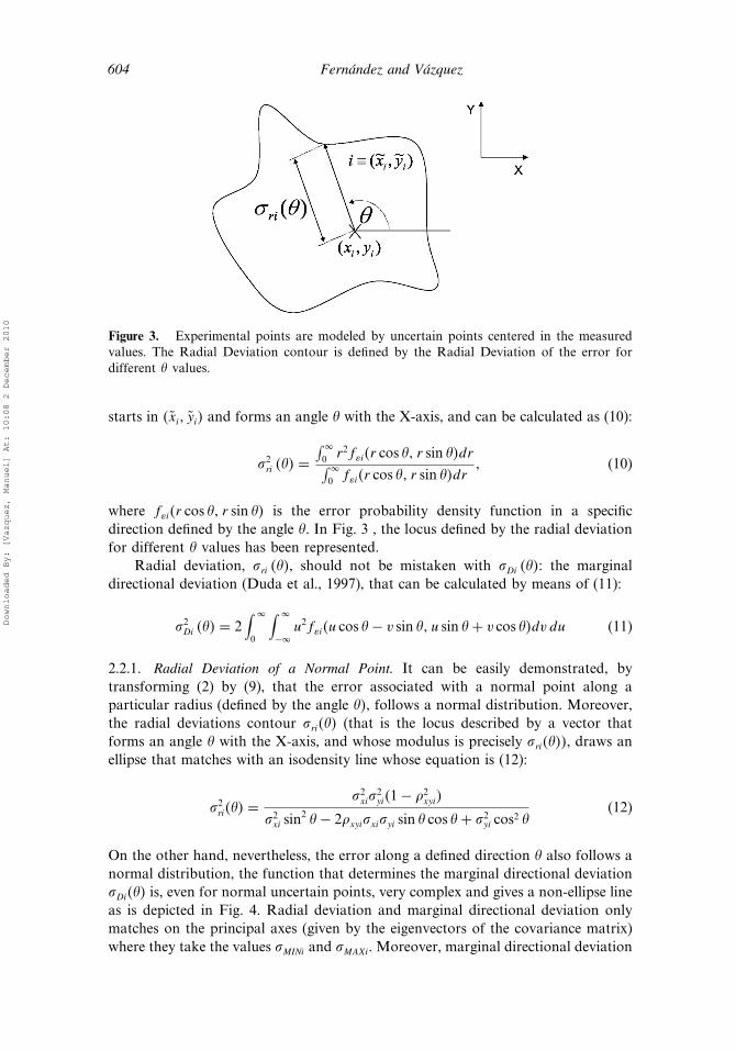
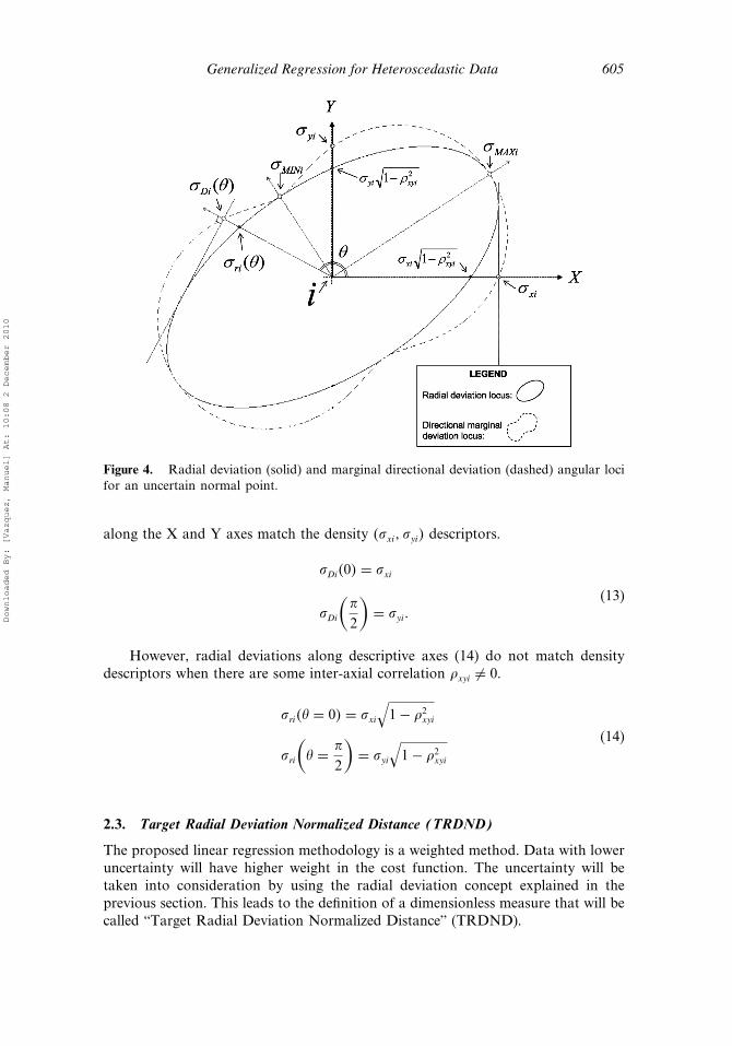
On the other hand, nevertheless, the error along a defined direction � also follows anormal distribution, the function that determines the marginal directional deviation�Di�� is, even for normal uncertain points, very complex and gives a non-ellipse lineas is depicted in Fig. 4. Radial deviation and marginal directional deviation onlymatches on the principal axes (given by the eigenvectors of the covariance matrix)where they take the values �MINi and �MAXi. Moreover, marginal directional deviation



Figure 4. Radial deviation (solid) and marginal directional deviation (dashed) angular locifor an uncertain normal point.

along the X and Y axes match the density ��xi� �yi� descriptors.

�Di�0� = �xi

�Di

(�

2

)= �yi

(13)

However, radial deviations along descriptive axes (14) do not match densitydescriptors when there are some inter-axial correlation �xyi �= 0.

�ri�� = 0� = �xi

√1− �2

xyi

�ri

(� = �

2

)= �yi

√1− �2

xyi

(14)

2.3. Target Radial Deviation Normalized Distance (TRDND)

The proposed linear regression methodology is a weighted method. Data with loweruncertainty will have higher weight in the cost function. The uncertainty will betaken into consideration by using the radial deviation concept explained in theprevious section. This leads to the definition of a dimensionless measure that will becalled “Target Radial Deviation Normalized Distance” (TRDND).



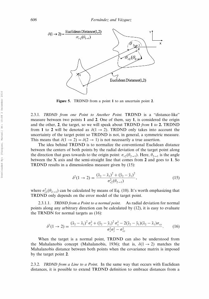
Figure 5. TRDND from a point 1 to an uncertain point 2.

2.3.1. TRDND from one Point to Another Point. TRDND is a “distance-like”measure between two points 1 and 2. One of them, say 1, is considered the originand the other, 2, the target, so we will speak about TRDND from 1 to 2. TRDNDfrom 1 to 2 will be denoted as ��1 → 2�. TRDND only takes into account theuncertainty of the target point so TRDND is not, in general, a symmetric measure.This means that ��1 → 2� = ��2 → 1� is not necessarily a true assertion.

The idea behind TRDND is to normalize the conventional Euclidean distancebetween the centers of both points by the radial deviation of the target point alongthe direction that goes towards to the origin point: �r2��2→1�. Here, �2→1 is the anglebetween the X axis and the semi-straight line that comes from 2 and goes to 1. SoTRDND results in a dimensionless measure given by (15):

�2�1 → 2� = �x2 − x1�2 + �y2 − y1�

2

�2r2��2→1�

� (15)

where �2r2��2→1� can be calculated by means of Eq. (10). It’s worth emphasizing that

TRDND only depends on the error model of the target point.

2.3.1.1. TRDND from a Point to a normal point. As radial deviation for normalpoints along any arbitrary direction can be calculated by (12), it is easy to evaluatethe TRNDN for normal targets as (16):

�2�1 → 2� = �x2 − x1�2 �2

y + �y2 − y1�2 �2

x − 2�y2 − y1��x2 − x1��xy

�2x�

2y − �2

xy

(16)

When the target is a normal point, TRDND can also be understood fromthe Mahalanobis concept (Mahalanobis, 1936); that is, ��1 → 2� matches theMahalanobis distance between both points when the covariance matrix is imposedby the target point 2.

2.3.2. TRDND from a Line to a Point. In the same way that occurs with Euclideandistances, it is possible to extend TRDND definition to embrace distances from a



line to a target point. We will consider TRDND from a line r, to a target point, ias the minimum TRDND from all the points R ∈ r to the point i (17):

�2i r → i� = Minimum[�2 R → i� ∀R ∈ r

] (17)

According to (17), we can obtain an explicit equation for TRNDN from astraight line when the target is a normal point. By replacing straight line polardescriptors D�� in the TRDND Eq. (16) for the different points of the straight line(defined in terms of different values of �R� and the datum i defined as a normaluncertain point we obtain (18):

�2 R → i� = 11− �2

xyi

(�D cos��− xi − sin��R�

2

�2x

+ �D sin��− yi + cos��R�2

�2y

− 2 �D sin��− yi + cos��R� �D cos��− xi + sin��R� �xy

�x�y

)(18)

Constraining the derivative with respect to �R of this function to be zero, we canevaluate �RMIN , the value that identifies the point of the straight line that minimizesthe TRDND. Eventually, by replacing the obtained value of �RMIN in (18) we obtainthe TRDND from the straight line to a normal point as (19):

�2 r → i� = �−D + cos��xi + sin��yi�2

�2xicos2��+ �xyi

�xi�yi

sin�2��+ �2yisin2��

= �−D + cos��xi + sin��yi�2

�2i

(19)

Equation (19) allows interpreting � r → i� as the Euclidean distance between theline and the point, divided by a partition value: �i (20) that does not depend on D:

�2i = �2

xicos2��+ �xyi

�xi�yi

sin�2��+ �2yisin2�� (20)

It’s worth mentioning that �i does not match, in general, with marginal directionaldeviation (11) nor radial deviation (12).

2.3.3. TRDND from One Line to a Cloud of Points. Following the same strategy,we can define the squared TRDND from a line: r, to a cloud: I = 1� 2 i n�:�2 r → I� to be equal to the variance residual (21):

�2 r → I� = 1n− 2

∑i∈I

�2�r → i� (21)

If we call Q2i to the squared TRDND from the straight line to the datum i, we have:

Q2i = �2�r → i� (22)



By simply applying this definition to (21), we have (23):

�2 r → I� = 1n− 2

∑i∈I

Q2i (23)

� r → I� can be understood as a measure of the dissimilarity between a line rand a cloud I , that takes into account the uncertainties of the cloud’s points in thedirection that points to r. In particular, if the points of I lie on r, then � r → I� = 0.

For straight lines and normal clouds we can use (19) to obtain (24):

Q2i =

�−D + cos��xi + sin��yi�2

�2i

(24)

3. TRDND Formulation of Regression Problems

Given a cloud I , made up of n points I = 1� 2� 3� i n�, the proposedmethodology reduces the regression problem to the problem of finding theline rguess ≡ �Dguess� �guess� that minimizes TRDND from rguess to I . The couple�Dguess� �guess� can be evaluated by forcing the derivatives of (23) to zero. Thus, weobtain the constraints (25):

��2[rguess → I

]�Dguess

= 0

��2[rguess → I

]��guess

= 0 (25)

As there is one constraint for each unknown, the system has a well-defined straightline solution.

As it has been explained above, this methodology constitutes a generalizedframework that can be particularized to reproduce classical straight line regressionresults. Typically, these particularizations are the normality of the clouds, besidesothers common sense assumptions about means and variances. For example, wecan obtain BLS cost function by using our methodology under the normal cloudhypothesis, by using Eq. (19), and reformulating it by substituting the polardescriptors �D�� by the classical slope-y intercept descriptors �m� b� with the helpof the transformations (26):

D = b sin��

m = −ctg�� (26)

That leads to Eq. (27):

�2 r → i� = �yi −mxi − b�2

�2yi − 2b�xyi + b2�2

xi

(27)

(27) is formally identical to BLS formula (7) of Sayago et al. (2004), so ourmethodology gives the same results than BLS if we assume:

(a) The normality of the cloud.



(b) The identification between the squared standard deviations of marginal errordensities ��2

xi� �2yi� and the variances �s2xi� s

2yi� supplied to BLS.

(c) The identification between the expected values of data densities and themeasured values supplied to BLS.

Other classical methods can be obtained in a similar way. Table 1 showsthe assumptions that must be done in order to force the results of the proposedmethodology to be the same that are obtained by some classical methods. However,even for these cases, the improved robustness that comes from the use of polardescriptors for straight lines and from the unifications of multiple methods in asingle algorithm gives a clear advantage to the methodology:

4. PDIM: An Iterative Method for Solving the Regression Problem

In this section, a numerical algorithm: PDIM (Polar Descriptors Iterative Method)will be developed for solving straight line fitting regression problems based inthe proposed methodology for normal clouds. According to the former section,our objective is to find the straight line rguess ≡ �Dguess� �guess� that minimizes�2[rguess → I

](23). As 1

n−2 is a constant factor for a given problem, it will be enoughto minimize the cost function Q2 defined by (28):

Q2 =∑i∈I

Q2i (28)

Under the assumption of normal clouds, the partition values �i (20) are allpolynomials of degree two in z = cos� that can have different factorization foreach datum. So the sum Q2 becomes an algebraic fraction whose numerator’s degreecan grow up to a value of 2n, making the algebraic resolution intractable even forlow n values. PDIM must be therefore an approximate method.

The main idea behind PDIM is to determine a succession of k straight linesr k� ≡ �D k�� k�� that goes in the proximity of a minimum of (28), �Dguess� �guess�,as the succession index k grows. To do that, in each step k, we will find the values�D k�� k�� that minimize (29):

Q2 k� =∑i∈I

Q2i k� =

∑i∈I

�xi cos�� k��+ yi sin�� k��−Di k��2

�2i k− 1�

(29)

Equation (29) assumes that the actual partition values �i k� can beapproximated by its previous values: �i k− 1� ≈ �i k�. Moreover, �i k− 1� dependsonly on the angle descriptor of the previous regression line: � k− 1�, and can becalculated at the beginning of the kth step by means of (30):

�2i k− 1� = �2

xicos2�� k− 1��+ �xyi

�xi�yi

sin�2� k− 1��

+ �2yisin2�� k− 1�� (30)

This assumption maintains all the denominators of (29) independent of theactual step descriptors, �D k�� k��, so we can add all its the terms in ahomogeneous way in order to obtain an algebraically solution for �D k�� k��.



The validity of (29) can be justified by the following fact: if we derive (29)with respect to �D k�� k��, and constrain them to be zero, we get to a set of twoequations that let us to determine �D k�� k�� as a function of �D k− 1�� k− 1��.It is clear that if the succession r k� stabilizes, then � k� � k− 1� and D k� D k− 1�. In particular, by (30), this means that the condition �i k− 1� �i k� isfulfilled and (29) is valid. Therefore, the convergence of �D k�� k�� is a criterionfor both: the stationary character of the limit, and the validity of (29).

By making the derivative of (29) with respect to D k�, we get a first constrain(31):

0 = −12

�

�D k�Q2

i k� =∑i∈I

−12

�

�D k�Q2

i k�

= ∑i∈I

xi cos�� k��+ yi sin�� k��−D k�

�2i k− 1�

(31)

Now, in order to simplify the equations we define the following momenta (32):

�i k� =1

�i k�

�gg k� =∑i∈I

�2i k�

�xgg k� =∑i∈I

xi�2i k�

�ygg k� =∑i∈I

yi�2i k�

�xxgg k� =∑i∈I

x2i �2i k�

�xygg k� =∑i∈I

xiyi�2i k�

�yygg k� =∑i∈I

y2i �2i k�

(32)

These conventions let us add (31) and express it as:

0 = �xgg k− 1� cos�� k��+ �ygg k− 1� sin�� k��− �gg k− 1�D k� (33)

Isolating D k� in (31), we have:

D k� = �xgg k− 1� cos�� k��+ �ygg k− 1� sin�� k��

�gg k− 1� (34)

Now, we build a second constrain by forcing the derivative of (29), now withrespect to � k�, to be zero.

0 = 12

�

�� k�Q2 k� =∑

i∈I

12

�

�� k�Q2

i k� (35)



That yields:

0 =∑i∈I

�−xi sin�� k��xi + yi cos�� k�� xi cos�� k��+ yi sin�� k��−D k��

�2i k− 1�

(36)

Substituting the value of D k� given by (34) into (36), grouping the terms withthe same dependence on � k� and using the momenta defined in (32), we come, aftersome algebra stuff, to (37):

0 =(�xygg k− 1�− �xgg k− 1��ygg k− 1�

�gg k− 1�

)cos2�� k��

−(�xygg k− 1�− �xgg k− 1��ygg k− 1�

�gg k− 1�

)sin2�� k��

+(�yygg k− 1�− �xxgg k− 1�+ �2xgg k− 1�− �2ygg k− 1�

�gg k− 1�

)sin�� k�� cos�� k��

(37)

And now by calling

A k− 1� = �xygg k− 1�− �xgg k− 1��ygg k− 1�

�gg k− 1�

B k− 1� = 12

(�yygg k− 1�− �xxgg k− 1�+ �2xgg k− 1�− �2ygg k− 1�

�gg k− 1�

)�

(38)

we can simplify (37) by using (38) in the form (39):

0 = A k− 1�(cos2�� k��− sin2�� k��

)+ 2B k− 1� sin�� k�� cos�� k�� (39)

Now, by using the trigonometric formulae for double angle, we can write (39)in an even more synthetic way.

0 = A k− 1� cos�2� k��+ B k− 1� sin�2� k�� (40)

So the system (31), (35), has an analytic solution given by (41) and (42):

� k� = 12Arc tan

(−B k− 1�A k− 1�

)+ p

�

2�with p ∈ Z� (41)

D k� = �xgg k− 1� cos�� k��+ �ygg k− 1� sin�� k��

�gg k− 1� (42)

The solution for � k�: (41), has four discernible branches corresponding to thevalues of p ∈ 0� 1� 2� 3�. The last task in each step should be to select which of themactually corresponds to the minimum of Q k�.

Each one of the � k� solutions leads to a corresponding D k� value by Eq. (42).From among these four solutions, two of them give negative values for D k�, so theyare nonsense. Focusing on the other two, one of them corresponds to a maximum,



and the other to a minimum. In order to select the minimum, we have to comparethe cost function value for both solutions, and select the solution that gives the costfunction Q k� whose value is the smallest. So, in order to perform the selection,it is required to obtain Q k� as a function of the momenta (32). We can do it byexpanding (29) in a sum of terms, and doing the sum of the series by using themomenta (32). That yields (43):

Q2 k� = �xxgg k� cos2�� k��+ 2�xygg k� cos�� k�� sin�� k��

+ �yygg k� cos2�� k��− 2�xgg k�D k� cos�� k��

− 2�ygg k�D k� sin�� k��+ �gg k�D2 k� (43)

Equation (43) is also suited for calculating the TRDND from the regression lineto the cloud � r → I�, which constitutes a quality measurement of the regression.

Once having Q, TRDND can be calculated as: � r → I� = 1√n−2

Q.It is convenient to point out that this scheme does not assure the succession

convergence towards the desired minimum. Depending on the initial value ofdescriptors, the succession could diverge or be chaotic. Moreover, if the data are illconditioned and the cost function has multiple minima, it can go towards a localminimum different to the desired absolute minimum.

So, it is required to explore the descriptor’s initial value space in order toreject the non convergent successions and select, among the convergent ones, theone that gives place to the least value of the cost function (43). Anyway, thisexploration process is greatly simplified by the fact that the succession has beencarefully constructed in such a way that its dynamic is fully determined by theinitial value of the single � descriptor,� 0�, because in each step, the D k� descriptorcomes algebraically determined by the � k� value through (42). This reduces theexploration to the one-dimensional interval: � 0� ∈ 0� 2��.

5. Evaluation and Results

In this section, we will show the scheme that was developed in order to evaluatelinear regression methods, and its application to highlight PDIM features undersome quite general conditions.

Monte Carlo techniques are used in order to synthesize trial clouds that follow adesired profile. The objective is to achieve a good (understandable and controllable)parameterization of clouds’ behavior.

In order to fulfil this goal, the scheme takes advantage of polar description oflinear laws. Uncertain points are constructed by selecting randomly at the beginningtheir deflection angles � seen from the origin (Fig. 2), and then using (7) in order toobtain the coordinates of its centers, (instead of starting from choosing at randomone single coordinate (x or y�, and using (4) or (5) in order to determine the otherone, as is done usually). This strategy has two advantages.

1. Any underlying linear law can be modeled, including lines that are parallel to theY-axis.

2. The cloud scattering profile description gets decoupled from the underlying law.That is: the clustering features of the clouds can be specified without taking intoaccount the slope of the law or the axis system on which the data are given.



Another feature of the scheme is the use of logarithms units (dB) for all positivedescriptors and error measures; it has the advantage of widening the range ofsituations that are described in the graphs, and isolating their interpretations fromthe units on which data are given.

5.1. Evaluation Procedure and Cloud Synthesis

The guidelines of the evaluation procedure are depicted in Fig. 6. A population It�of T clouds (1 ≤ t ≤ T� is synthesized by Monte Carlo techniques, according with aset of eleven real parameters (cloud profile) that describe statistically the features ofthe kind of cloud against which one want to test the methodology.

These 11 cloud profile descriptors (that appears in the leftmost box inside thepopulation box of Fig. 6), can be grouped in four groups: from below to above:

(1) The true law descriptors rtrue ≡ �Dtrue� �true� that determines the line where thedata centres lie.

(2) The number of points n that make up the clouds, and the flare angle interval �min� �max�, that is the range of angles seen from the origin (and measured withrespect to the direction of the nearest point of the true law line) from where thedata centres can be chosen (see Fig. 2). Thus, the flare angle interval controlsdirectly the asymmetry of the cloud with respect to the nearest point and theamount of dispersion of data centers along the law line.

Figure 6. Test methodology explanatory diagram.



(3) The descriptors of the uncertainty degree of the points of the cloud, namely theallowed interval for inter-axial cross correlation �min� �max�, and the minimumallowed value of the deviation along each data axis: �xmin�dB�, and �ymin�dB�.The deviations are given in logarithms units (with respect to the unit measureof Dtrue�; that is (44):

�xmin�dB� = 20Log10��xmin�

�ymin�dB� = 20Log10��ymin�(44)

(4) The descriptors of the heteroscedasticity degree. These are the amplitude marginof directional deviation of error on X and Y directions: �xmargin and �ymargin.These two values are also supplied in dB, so the maximum values ��xmax� �ymax�

of the directional deviations in dB can be calculated as (45):

�xmax�dB� = �xmin�dB�+ �xmargin�dB�

�ymax�dB� = �ymin�dB�+ �ymargin�dB�(45)

Once the cloud profile descriptors have been established, a statistical modelingof each one of its points (central box inside the population box of Fig. 6) issynthesized by fulfilling the cloud profile. This is done by selecting at random foreach point i of the cloud, the following descriptors:

(1) The uncertain point centers, (that lie exactly on the law). This selection requireschoosing previously a set �i of n angles uniformly inside the flare angle interval �min� �max�. Once the �i have been chosen, the coordinates of data centres�xi� yi� can be evaluated by (46):

{xi = Dtrue cos��true�−Dtrue sin��true� tan��i�

yi = Dtrue sin��true�+Dtrue cos��true� tan��i�(46)

(2) The value of the inter-axial cross correlations �xyi associated with each uncertainpoint. These are chosen uniformly inside the cloud profile interval �min� �max�.

(3) The value of the directional deviation of error on X and Y directions, �xi� �yi

associated with each uncertain point. These values are choosing at randomaccording with a log-uniform distribution inside the ranges �xmin� �xmax� and �ymin� �ymax�. In fact, this is done by choosing �xi�dB�� yi�dB� uniformly inside �xmin�dB�� xmax�dB�� and �ymin�dB�� ymax�dB��, and then getting �xi� �yi bysimply converting �xi�dB�� yi�dB� to linear units by

�xi�dB� = 10�xi�dB�

20

�yi�dB� = 10�yi�dB�

20 (47)

Now, one has a statistical description of each uncertain point of the cloud madeup of five parameters: xi� yi� �xi� �yi� �xyi�. The last step (rightmost box inside thepopulation box of Fig. 6) in the synthesis is to generate a noised sample �xi� yi� for



each point. For doing this, some noise ��xi� �yi� is added (48) to the data centers�xi� yi�.

xi = xi + �xi

yi = yi + �yi(48)

The noise is chosen at random, according with a zero mean normal bivariatedistribution whose covariance matrix for each point �i is given by (49):

�i =(

�2xi �xyi�xi�yi

�xyi�xi�yi �2yi

) (49)

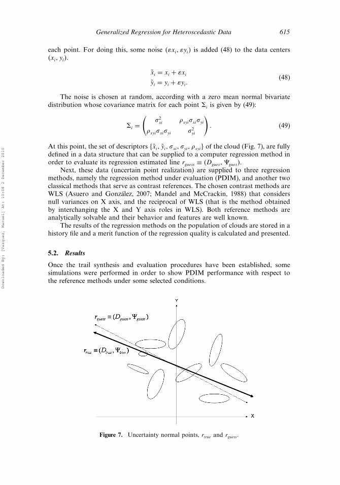
At this point, the set of descriptors xi� yi� �xi� �yi� �xyi� of the cloud (Fig. 7), are fullydefined in a data structure that can be supplied to a computer regression method inorder to evaluate its regression estimated line rguess ≡ �Dgues� �gues�.

Next, these data (uncertain point realization) are supplied to three regressionmethods, namely the regression method under evaluation (PDIM), and another twoclassical methods that serve as contrast references. The chosen contrast methods areWLS (Asuero and González, 2007; Mandel and McCrackin, 1988) that considersnull variances on X axis, and the reciprocal of WLS (that is the method obtainedby interchanging the X and Y axis roles in WLS). Both reference methods areanalytically solvable and their behavior and features are well known.

The results of the regression methods on the population of clouds are stored in ahistory file and a merit function of the regression quality is calculated and presented.

5.2. Results

Once the trail synthesis and evaluation procedures have been established, somesimulations were performed in order to show PDIM performance with respect tothe reference methods under some selected conditions.

Figure 7. Uncertainty normal points, rtrue and rguess.



All tests in this section were obtained following steps below.

1. Imposing the fixed cloud descriptors values according with the selectedconditions, and the number of trial clouds T we are going to use for theestimation at each point of the graph.

2. Looping the variable descriptor values, i.e. the values of the cloud descriptorswhose impact on the performance is going to be evaluated.

3. Calculating the merit function of interest by using the history file rguesst� and theprevious known goal law rtrue.

4. Displaying the merit function on the vertical axis as a function of the variableparameter on the horizontal axis.

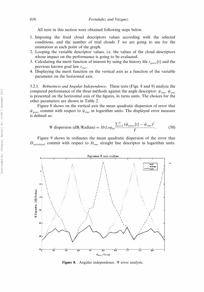
5.2.1. Robustness and Angular Independence. These tests (Figs. 8 and 9) analyze thecompared performance of the three methods against the angle descriptor: �true. �true

is presented on the horizontal axis of the figures, in turns units. The choices for theother parameters are shown in Table 2.

Figure 8 shows on the vertical axis the mean quadratic dispersion of error that�guess commit with respect to �true in logarithm units. The displayed error measureis defined as:

� dispersion (dB/Radian) = 10Log10

∑Tt=1 ��guesst�− �true�

2

T (50)

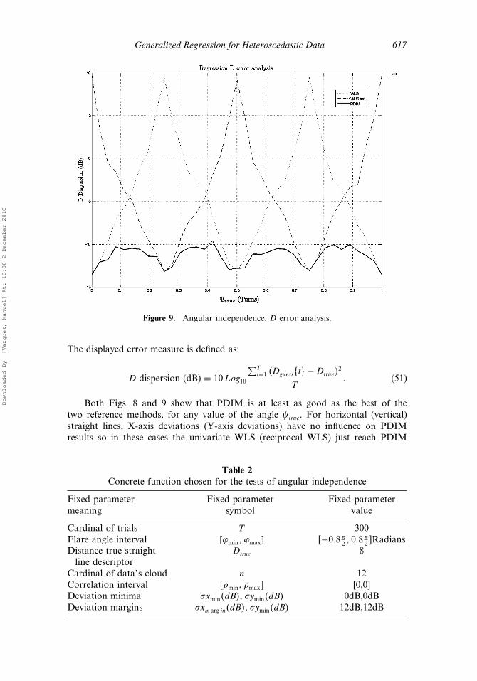
Figure 9 shows in ordinates the mean quadratic dispersion of the error thatDcalculated commit with respect to Dtrue straight line descriptor in logarithm units.

Figure 8. Angular independence. � error analysis.



Figure 9. Angular independence. D error analysis.

The displayed error measure is defined as:

D dispersion (dB) = 10Log10

∑Tt=1 �Dguesst�−Dtrue�

2

T (51)

Both Figs. 8 and 9 show that PDIM is at least as good as the best of thetwo reference methods, for any value of the angle �true. For horizontal (vertical)straight lines, X-axis deviations (Y-axis deviations) have no influence on PDIMresults so in these cases the univariate WLS (reciprocal WLS) just reach PDIM

Table 2Concrete function chosen for the tests of angular independence

Fixed parametermeaning

Fixed parametersymbol

Fixed parametervalue

Cardinal of trials T 300Flare angle interval [�min� �max] −08 �

2 � 08�2 �Radians

Distance true straightline descriptor

Dtrue 8

Cardinal of data’s cloud n 12Correlation interval �min� �max� [0,0]Deviation minima �xmin�dB�� ymin�dB� 0dB,0dBDeviation margins �xm arg in�dB�� ymin�dB� 12dB,12dB



results. For other �true values, the performance of the PDIM improves significantlyany of the reference methods results.

Although PDIM is fully isotropic, a residual 3dB fluctuation of performanceremains in both figures. This does not come from PDIM but from some bias thathas its origin in the trial cloud synthesis methodology, due to the fact that deviationminima and margins are referred to a specific axes descriptive system (X, Y).

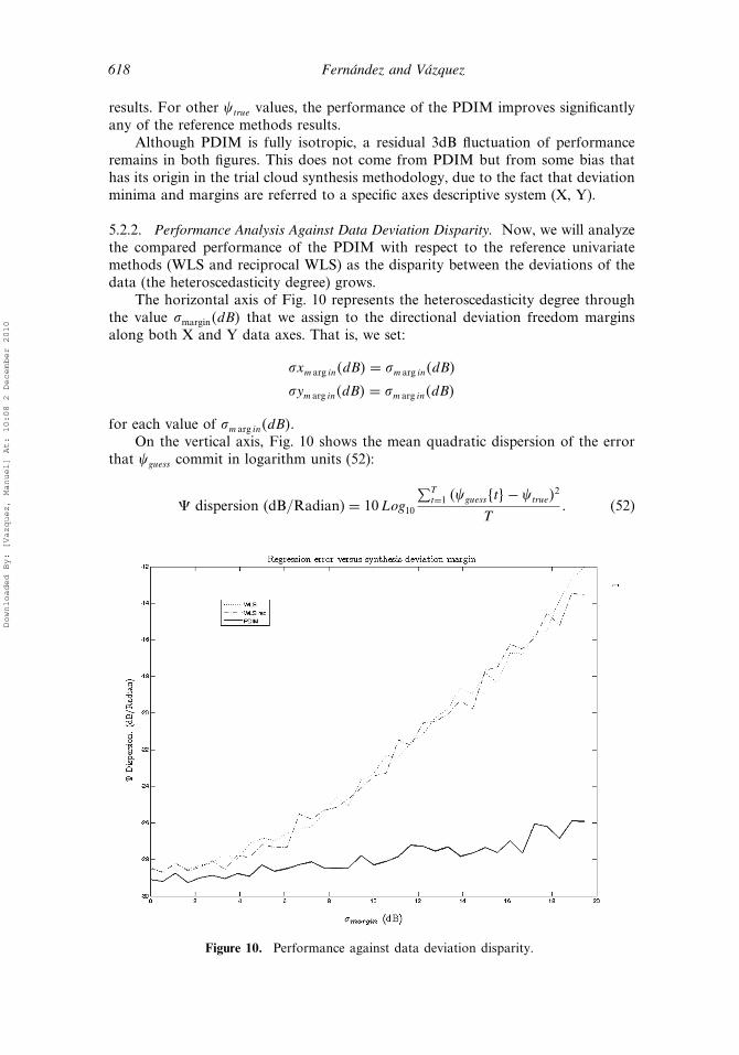
5.2.2. Performance Analysis Against Data Deviation Disparity. Now, we will analyzethe compared performance of the PDIM with respect to the reference univariatemethods (WLS and reciprocal WLS) as the disparity between the deviations of thedata (the heteroscedasticity degree) grows.

The horizontal axis of Fig. 10 represents the heteroscedasticity degree throughthe value �margin�dB� that we assign to the directional deviation freedom marginsalong both X and Y data axes. That is, we set:

�xm arg in�dB� = �m arg in�dB�

�ym arg in�dB� = �m arg in�dB�

for each value of �m arg in�dB�.On the vertical axis, Fig. 10 shows the mean quadratic dispersion of the error

that �guess commit in logarithm units (52):

� dispersion (dB/Radian) = 10Log10

∑Tt=1 ��guesst�− �true�

2

T (52)

Figure 10. Performance against data deviation disparity.



Table 3Concrete function chosen for the tests of performance against data deviation

disparity






Distance true straightline descriptor

Dtrue 8

Angle true straightline descriptor

�true �/4

Cardinal of cloud’s data n 12Correlation interval �min� �max� [0,0]Deviation minima �xmin�dB�� ymin�dB� 0dB,0dB

The choices for the others trial parameters are shown in Table 3.

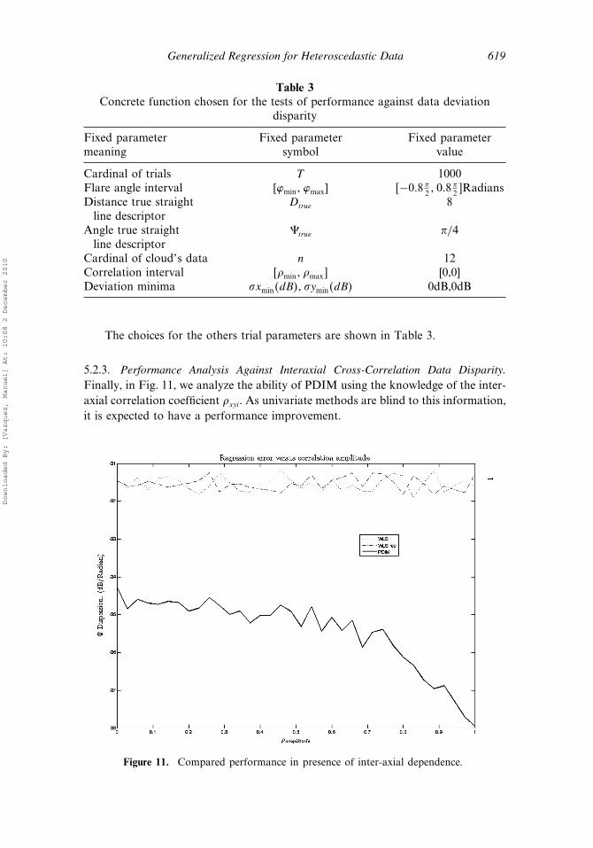
5.2.3. Performance Analysis Against Interaxial Cross-Correlation Data Disparity.Finally, in Fig. 11, we analyze the ability of PDIM using the knowledge of the inter-axial correlation coefficient �xyi. As univariate methods are blind to this information,it is expected to have a performance improvement.

Figure 11. Compared performance in presence of inter-axial dependence.



Table 4Concrete function chosen for the tests of performance against interaxial disparity






Distance straightline descriptor

Dtrue 8

Angle straightline descriptor

�true �/4

Cardinal of data’s cloud n 12Deviation minima �xmin�dB�� ymin�dB� 6dB,6dBDeviation margins �xm arg in�dB�� ymin�dB� 0dB,0dB

In the test, the interval of allowed values of �xyi, �min� �max� was selected by theformula

�min� �max� = −�amplitude� �amplitude��

Here, �amplitude is the inter-axial correlation amplitude freedom that is the variablethat has been represented on the horizontal axis of Fig. 11. On the vertical axis, thesame performance measure (52) of former results has been represented.

As inter-axial correlation amplitude freedom grows, it is expected that theperformance also grows, as effectively occurs in the graph. It can also be observedthat even for the �amplitude = 0 value, there is a 3dB gain of PDIM against univariatemethods. This 3dB improvement is due to the advantage that gives to PDIM theknowledge of the deviations on the two axes.

6. Conclusions

When data are scarce or experiments are expensive, it is important to take advantageof all the available knowledge about the quality of the measurements by usingsophisticated regression methods in order to improve the accuracy of the results.

In this article, we presented a regression methodology that is able to convert anystatistically formulated regression problem into a scalar optimization. It can dealwith arbitrary data error distribution functions and can be particularized, by makingsome simple additional assumptions in order to mimic classic regression methods asTLS, WLS, or BLS by a single algorithm.

The methodology is based on the definition of a measure (TRDND) on the dataspace and the use of polar descriptors �D�� for the straight lines, instead of theusual “slope, y-intercept” �m� b� descriptors. Polar descriptors avoid overflows forvertical lines, and isolate regression results from the concrete selection of axes onwhich the data are given.

Finally, a practical algorithm: PDIM was also developed in order to solve theproblem that arises when the methodology is applied to normal clouds. PDIM isable to advantageously afford the most complex cases of bivariate heteroscedasticdata with inter-axial dependence.



PDIM was tested and compared against others heteroscedastic univariatemethods that have singularities when laws are vertical or horizontal straight lines.It avoids these singularities and offers the best performance irrespective of theregression line slope.

PDIM results have been found to be especially profitable when dealing withdata that have a strong heteroscedasticity degree affecting both components and/orwith data subject to inter-axial dependence.

References

Asuero, G., González, G. (2007). Fitting straight lines with replicated observations by linearregresión. III. Weighting data. Crit. Rev. Analyt. Chem. 37:143–172.

Cheng, C., Riu, J. (2006). on estimating linear relationships when both variables are subjectto heteroscedastic measurement errors. Technometrics 48:511–519.

Duda, R. O., Hart, P. E., Store, D. G. (1997). Pattern Classification. New York: WileyInterscience.

González, J. R., Vázquez, M., Núñez, N., Algora, C., Rey-Stolle, I., Galiana, B. (2009).Reliability analysis of temperature step-stress tests on III–V high concentrator.Microelectronics Reliability 49:673–822.

Mahalanobis, P. C. (1936). On the generalised distance in statistics. Proc. Nat. Instit. Sci.India 12:49–55.

Mandel, J., McCrackin, F. L. (1988). An iterative self-weighting procedure for fitting straightlines to heteroscedastic data. Commun. Statist. Simul. Computat. 17(2):609—635.

Markovsky, I., Van Huffel, S. (2007). Overview of total least-squares methods. SignalProcess. 87:2283–2302.

Martínez, A., del Río, F. J., Riu, J., Rius, F. X. (1999). Detecting proporcional and constantbias in method comparison studios by using linear regression with errors in both axes.Chemometr. Intelligent Lab. Syst. 49:181–195.

Rawlings, J. O., Pantula, S. G., Dickey, D. A. (1998). Applied Regression Analysis: A ResearchTool. 2nd ed. New York: Springer Text in Statistics.

Sayago, A., Boccio, M., Asuero, A. G. (2004). fitting straight lines with replicatedobservations by linear regresión: the least squares postulates. Crit. Rev. Analyt. Chem.34:39–50.

Van Huffel, S., Cheng, C., Mastronardi, N., Paige, C., Kukush, A. (2007). Total least squaresand errors-in-variables modelling. Computat. Statist. Data Anal. 52:1076–1079.

Vázquez, M., Algora, C., Rey-Stolle, I., Algora, C. (2007). III–V concentration solar cellreliability prediction based on quantitative led reliability data. Prog. Phot. Res. Appl.15:477–491.

Wilcox, R. R. (2009). Robust multivariate regression when there is heteroscedasticity.Commun. Statist. Simul. Computat. 38(1):1–13.

Yu, Q., Chappell, R., Wong, G. Y. C., Hsu, Y., Mazur, M. (2008). Relationship between thecox, lehmann, weibull, and accelerated lifetime models. Commun. Statist. Theor. Meth.37(9):1458–1470.


Documents

Communications in Statistics - Theory and Methods A ... · Straight lines are managed through their polar descriptors D , instead of the usual “slope, y-intercept” mb descriptors