Embed Size (px)
Citation preview

Community Detection in Social Networks: Multilayer Networks and Pairwise Covariates
Sihan Huang
Submitted in partial fulfillment of therequirements for the degree of
Doctor of Philosophyunder the Executive Committee
of the Graduate School of Arts and Sciences
COLUMBIA UNIVERSITY
2020

© 2020
Sihan Huang
All Rights Reserved
Abstract
Community Detection in Social Networks: Multilayer Networks and Pairwise Covariates
Sihan Huang
Community detection is one of the most fundamental problems in network study. The
stochastic block model (SBM) is arguably the most studied model for network data with different
estimation methods developed with their community detection consistency results unveiled. Due
to its stringent assumptions, SBM may not be suitable for many real-world problems. In this
thesis, we present two approaches that incorporate extra information compared with vanilla SBM
to help improve community detection performance and be suitable for applications.
One approach is to stack multilayer networks that are composed of multiple single-layer
networks with common community structure. Numerous methods have been proposed based on
spectral clustering, but most rely on optimizing an objective function while the associated
theoretical properties remain to be largely unexplored. We focus on the ‘early fusion’ method
[114], of which the target is to minimize the spectral clustering error of the weighted adjacency
matrix (WAM). We derive the optimal weights by studying the asymptotic behavior of
eigenvalues and eigenvectors of the WAM. We show that the eigenvector of WAM converges to a
normal distribution as in [129], and the clustering error is monotonically decreasing with the
eigenvalue gap. This fact reveals the intrinsic link between eigenvalues and eigenvectors, and thus
the algorithm will minimize the clustering error by maximizing the eigenvalue gap. The
numerical study shows that our algorithm outperforms other state-of-art methods significantly,
especially when signal-to-noise ratios of layers vary widely. Our algorithm also yields higher

accuracy result for S&P 1500 stocks dataset than competing models.
The other approach we propose is to consider heterogeneous connection probabilities to
remove the strong assumption that all nodes in the same community are stochastically equivalent,
which may not be suitable for practical applications. We introduce a pairwise covariates-adjusted
stochastic block model (PCABM), a generalization of SBM that incorporates pairwise covariates
information. We study the maximum likelihood estimates of the coefficients for the covariates as
well as the community assignments. It is shown that both the coefficient estimates of the
covariates and the community assignments are consistent under suitable sparsity conditions.
Spectral clustering with adjustment (SCWA) is introduced to fit PCABM efficiently. Under
certain conditions, we derive the error bound of community estimation under SCWA and show
that it is community detection consistent. PCABM compares favorably with the SBM or
degree-corrected stochastic block model under a wide range of simulated and real networks when
covariate information is accessible.

Table of Contents
List of Tables . . . . . . . . . . . . . . . . . . . . . . . . . . . . . . . . . . . . . . . . . . iv
List of Figures . . . . . . . . . . . . . . . . . . . . . . . . . . . . . . . . . . . . . . . . . . v
Acknowledgments . . . . . . . . . . . . . . . . . . . . . . . . . . . . . . . . . . . . . . . . vi
Dedication . . . . . . . . . . . . . . . . . . . . . . . . . . . . . . . . . . . . . . . . . . . . vii
Chapter 1: Introduction and Background . . . . . . . . . . . . . . . . . . . . . . . . . . . 1
1.1 Literature review . . . . . . . . . . . . . . . . . . . . . . . . . . . . . . . . . . . 1
1.2 Overview of the thesis . . . . . . . . . . . . . . . . . . . . . . . . . . . . . . . . . 5
1.3 Notation and terminology . . . . . . . . . . . . . . . . . . . . . . . . . . . . . . . 6
Chapter 2: Optimal Weights for Multilayer Networks . . . . . . . . . . . . . . . . . . . . 9
2.1 Introduction . . . . . . . . . . . . . . . . . . . . . . . . . . . . . . . . . . . . . . 9
2.2 Multilayer network model . . . . . . . . . . . . . . . . . . . . . . . . . . . . . . . 10
2.3 Theory and algorithms for the optimal weights . . . . . . . . . . . . . . . . . . . . 11
2.3.1 Closed-form solution for optimal weights . . . . . . . . . . . . . . . . . . 11
2.3.2 Eigenvalue gap optimization . . . . . . . . . . . . . . . . . . . . . . . . . 13
2.4 Simulations . . . . . . . . . . . . . . . . . . . . . . . . . . . . . . . . . . . . . . 15
2.4.1 MPPM setting . . . . . . . . . . . . . . . . . . . . . . . . . . . . . . . . 15
i

2.4.2 MSBM setting . . . . . . . . . . . . . . . . . . . . . . . . . . . . . . . . 18
2.5 Real data example . . . . . . . . . . . . . . . . . . . . . . . . . . . . . . . . . . . 19
2.6 Discussion . . . . . . . . . . . . . . . . . . . . . . . . . . . . . . . . . . . . . . . 23
2.7 Proofs . . . . . . . . . . . . . . . . . . . . . . . . . . . . . . . . . . . . . . . . . 23
2.7.1 Proof of Proposition 2.1 . . . . . . . . . . . . . . . . . . . . . . . . . . . 23
2.7.2 Proof of Proposition 2.3 . . . . . . . . . . . . . . . . . . . . . . . . . . . 31
Chapter 3: Pairwise Covariate-Adjusted Block Model . . . . . . . . . . . . . . . . . . . . 36
3.1 Introduction . . . . . . . . . . . . . . . . . . . . . . . . . . . . . . . . . . . . . . 36
3.2 PCABM setup . . . . . . . . . . . . . . . . . . . . . . . . . . . . . . . . . . . . . 38
3.3 Theory and algorithms for PCABM . . . . . . . . . . . . . . . . . . . . . . . . . . 39
3.3.1 Likelihood method . . . . . . . . . . . . . . . . . . . . . . . . . . . . . . 40
3.3.2 Spectral clustering with adjustment . . . . . . . . . . . . . . . . . . . . . . 44
3.4 Simulations . . . . . . . . . . . . . . . . . . . . . . . . . . . . . . . . . . . . . . 47
3.4.1 Coefficient estimation . . . . . . . . . . . . . . . . . . . . . . . . . . . . . 48
3.4.2 Community detection . . . . . . . . . . . . . . . . . . . . . . . . . . . . . 48
3.5 Real data examples . . . . . . . . . . . . . . . . . . . . . . . . . . . . . . . . . . 51
3.5.1 Example 1: political blogs . . . . . . . . . . . . . . . . . . . . . . . . . . 51
3.5.2 Example 2: school friendship . . . . . . . . . . . . . . . . . . . . . . . . . 52
3.6 Discussion . . . . . . . . . . . . . . . . . . . . . . . . . . . . . . . . . . . . . . . 55
3.7 Proofs . . . . . . . . . . . . . . . . . . . . . . . . . . . . . . . . . . . . . . . . . 57
3.7.1 Proof of Theorem 3.1 and Theorem 3.2 . . . . . . . . . . . . . . . . . . . 57
3.7.2 Some concentration inequalities and notations . . . . . . . . . . . . . . . . 59
ii

3.7.3 Proof of Theorem 3.3 . . . . . . . . . . . . . . . . . . . . . . . . . . . . . 64
3.7.4 Proof of Theorem 3.4 . . . . . . . . . . . . . . . . . . . . . . . . . . . . . 67
3.7.5 Proof of Theorem 3.5 . . . . . . . . . . . . . . . . . . . . . . . . . . . . . 68
Conclusion . . . . . . . . . . . . . . . . . . . . . . . . . . . . . . . . . . . . . . . . . . . 74
References . . . . . . . . . . . . . . . . . . . . . . . . . . . . . . . . . . . . . . . . . . . . 86
iii

List of Tables
2.1 Parameters of experiments under MPPM . . . . . . . . . . . . . . . . . . . . . . . 16
2.2 Parameters of experiments under MPPM for different scales . . . . . . . . . . . . . 17
2.3 Parameters of experiments under MSBM . . . . . . . . . . . . . . . . . . . . . . 19
3.1 Simulated results for distribution of γ, displayed as mean (standard deviation) . . . 49
3.2 Performance comparison on political blogs data . . . . . . . . . . . . . . . . . . . 52
3.3 Inference results when school is targeted community . . . . . . . . . . . . . . . . 54
3.4 Inference results when ethnicity is targeted community . . . . . . . . . . . . . . . 54
3.5 ARI comparison on school friendship data . . . . . . . . . . . . . . . . . . . . . . 55
iv

List of Figures
2.1 Eigenvalue gap versus SNR . . . . . . . . . . . . . . . . . . . . . . . . . . . . . . 14
2.2 ARI results from MPPM experiments . . . . . . . . . . . . . . . . . . . . . . . . 16
2.3 ARI results under different scales . . . . . . . . . . . . . . . . . . . . . . . . . . . 18
2.4 ARI results from MSBM experiments . . . . . . . . . . . . . . . . . . . . . . . . 20
2.5 Correlation adjacency matrices for different time windows . . . . . . . . . . . . . 21
2.6 Confusion matrices of different clustering methods . . . . . . . . . . . . . . . . . 22
3.1 Different network models including covariates . . . . . . . . . . . . . . . . . . . . 37
3.2 Simulation results for γ compared with theoretical values . . . . . . . . . . . . . . 49
3.3 Simulation results under PCABM for different parameter settings . . . . . . . . . . 50
3.4 Simulation results under DCBM for different parameter settings . . . . . . . . . . 51
3.5 Community detection with different pairwise covariates . . . . . . . . . . . . . . . 56
v

Acknowledgements
Foremost I wish to express my sincere appreciation to my advisor, Professor Yang Feng, for
his continuous guidance and encouragement. He taught me to be professional and find the right
direction when I am lost. Without his persistent help, this thesis would not have been possible.
I would like to thank Professor Haolei Weng for his suggestions for the second chapter.
Also, the serving of Professor Zhiliang Ying, Professor Tian Zheng, and Professor Daniel Hsu on
my committee is truly appreciated. Their insightful comments are valuable to improve my thesis.
I have been blessed with an accompany of numerous friends who gave me so much support
and joy. There are too many to thank by name, but I am especially grateful to Yang Kang, Liwei
Wu, Fan Shi, Yi Hong, Zhi Li, Yuanzhe Xu, Boyuan Zhang, Chaoyu Yuan and Jing Wu, whose
friendship has been so important to me throughout the hard periods of my life.
Finally, I wish to acknowledge the support and great love of my family: my parents Jian
Huang and Min Zhang, for giving birth to me and supporting me spiritually throughout my life.
vi

To my beloved parents who always support me to explore the possibilities of my life.
vii
Chapter 1: Introduction and Background
The network describes the connections among subjects in a population of interest. Its wide
applications have attracted researchers from different fields, which includes but not limited to so-
cial sciences [135, 93], physics [10], computer science [110], biology [79] and so on. Among
all problems for network, community detection is one of the most studied ones, and the stochas-
tic block model (SBM) has long been used as a canonical model for that. Although theoretical
properties of classical SBM have been studied thoroughly, the theoretical framework hasn’t been
established for its variants. We’re interested in the expanded version of SBM, say when there is
extract information beside the network edges, how we could exploit that information and make a
better inference.
We will review the history of network analysis in Section 1.1, especially focusing on the re-
searches of community detection and SBM. In Section 1.2, we provide an overview of our two
variants of SBM. Section 1.3 introduces some basic notations that will be used later.
1.1 Literature review
The very first researches for network date back to the middle of last century, marked by some
empirical studies in social psychology and sociology [104, 124, 103, 130]. The works in social sci-
ence ignite researchers’ passion for mathematical insights of network models. Erdos-Rényi model,
which became the canonical model in network analysis later, was first introduced in the 1960s [55].
The random graph theory that later arose was mostly based on that. People studied the asymptotic
behavior of the Erdos-Rényi model, which has n nodes and each edge is generated by the homoge-
neous probability p. The ‘phase transition’ that later became well-known associated with the value
of pn = 1, at which point many small clusters will merge into a single giant connected component.
1
Erdos-Rényi model was extended and generalized in the 1980s. The models have the most lasting
impact include but are not limited to p1 model [74, 60], multidimensional network structures [59],
SBM [73], exponential random graph models [64, 126, 136, 113, 118] and so on. More litera-
ture in the 1990s linked random graph models with stochastic processes and dig deeper into the
probabilistic properties [43, 52]. The machine learning approach is what emerged at the turn of
this century. Some empirical studies were done by [57, 83, 82, 84]. More recent efforts focus on
the variants of SBM. [72] combines SBM with latent space models. [70] introduced model-based
clustering. [8] includes the latent Dirichlet allocation [28] to provide a novel generative model,
which is a kind of soft clustering [56].
Communities in a network can be intuitively understood as groups of nodes that are densely
connected within groups while sparsely connected between groups. The goal of community detec-
tion is to partition the nodes into different sets. Not only does identifying network communities
help better understand the structural features of the network, but it also offers practical benefits.
Besides its original target to understand sociological behavior [67, 63], other applications of com-
munity detection have also been widely explored. Biologists classify protein function from the
protein-protein interaction network [7, 9, 38, 100]. By analyzing communication networks [18],
people can detect possible latent terrorist cells. With the emerging of online ‘networking com-
munities’ such as Facebook, Twitter and Instagram, the need for a recommender system based on
the similarity of nodes within the network also becomes nonnegligible [71, 94, 120, 140]. Other
applications include but are not limited to gene expressions [45, 77], natural language processing
[19], image segmentation [123] and more.
Classical community detection methods fall into three categories. The first category is algorithm-
based. One example is hierarchical clustering, which gradually removes edges until disconnected
clusters are obtained. More reviews can be found in [107]. The second category is criterion-based.
Such methods optimize some criterion to obtain the best partition of the network. This criterion
often refers to some cuts or modularities, which include Newman-Girvan modularity [109], the
ratio cut [137], the normalized cut [123] and more. The third category is model-based, which
2

is the main focus of this thesis. This kind of model builds a generative probabilistic model for
the network and tries to identify the latent community labels by fitting the model. Besides SBM
[125, 112] and mixed membership SBM that have been mentioned, other examples include degree-
corrected stochastic block models (DCBM) [80, 147], the latent position cluster model [70], latent
space model [72], etc. One thing that needs to remember is that those categories mentioned above
are just rough philosophical descriptions for different methods rather than strict divisions. For ex-
ample, we’ll see that the model in Chapter 3 can be both model-based and criterion-based, just like
[147, 24].
Among all the models, SBM might be the most natural one for describing the community
detection problem because of its neat form. Although the block structure of the network has already
been discussed as early as the 1970s [95], the random graph framework only came up a decade later
in [73], after numerous papers for deterministic blocks arose [14, 51, 50]. People in different fields
name it differently, for example, planted partition model (PPM) in theoretical computer science
[33, 53, 30], inhomogeneous random graph in math [29] and so on.
The enthusiasm for SBM theories mainly focuses on the consistency of community estimation.
Analogous to the concept of random variable convergence, for community detection, we have
strong consistency and weak consistency, which we will define in detail later. [49] pictured the
weak recovery in detail and conjectured that there exist phase transition phenomena for weak
consistency at the Kesten-Stigum threshold. The later activation of establishing phase transitions
should be credited to this paper. [106] proved the impossibility part of the conjecture for two
symmetric communities, while the positive part for two communities was shown in [101]. For
non-symmetric case, [31] proved that the threshold can be achieved under a more general setting
which covers asymmetric SBM of two communities. This borrows the idea from the ‘spectral
redemption’ paper [85], which introduces the nonbacktracking operator. More general cases for
arbitrarily many communities were shown in [3, 2], using a high-order nonbacktracking matrix and
a spectral-message passing. Crossing information-theoretic Kesten-Stigum threshold under more
communities were further discussed in [4, 17]. For exact recovery, the phase transition also exists,
3
though in the logarithmic rather than constant degree regime. For years, researchers worked on
this problem [33, 53, 30, 125, 46, 102, 24, 42, 133] until the sharp threshold was given in [1, 105]
for two symmetric communities. For general SBM, the parallel results were shown in [3, 5].
To efficiently perform inference for SBM under different settings, people designed various
algorithms. Some popular ones include modularity maximization [109], likelihood methods [24,
42, 147, 12, 35], spectral clustering [16, 119, 61, 78, 91, 122], variational inference [37, 26, 48,
35], belief propagation [49], convex optimization [41], semidefinite programming [1, 34, 108],
penalized local maximum likelihood estimation [65] and more.
Among all of them, spectral clustering stands out for its neat form and simplicity to implement,
so it’s long been a fascination for researchers. The detailed tutorial of spectral clustering can be
found in [132], and we just list a few important literature here. [119] proved the consistency for
spectral clustering with the normalized graph Laplacian, but it assumes the average degree grows
faster than log n. The same assumption holds in [78] and [122]. The former one proposed spectral
clustering on ratios-of-eigenvectors (SCORE) for the DCBM. The latter one compared normalized
and unnormalized spectral clustering. Shortly after, [91] proved consistency when the maximum
expected node degree is of order log n or higher. Also, an approximate k-means algorithm solvable
in polynomial time [86] is considered in [91] rather than the global optimizer of k-means. However,
on sparser graphs (e.g., average degree is of order O(1)), spectral clustering on standard graph
Laplacian performs poorly [37, 34, 13, 89], that’s where the regularized graph Laplacian came into
place [37]. It’s proven to misclassify at most arbitrarily small proportion of nodes [88]. There
are some other variants of spectral clustering for different purposes. [36] introduced the notion
of a degree-corrected graph Laplacian for the extended PPM. [61] required only an upper bound
of the number of communities for the modified adjacency matrix to guarantee the consistency
of spectral clustering. [117] applied the regularized graph Laplacian to the canonical spectral
clustering algorithm and provided the error bound for DCBM and extended PPM.
Besides what we’ve mentioned above, there are some other research topics on SBM’s variants
over the recent years. One concern is about the ‘outliers’ in the network, which refers to the node
4

that doesn’t belong to any group. Similar to regression, robust community detection algorithm is
proposed to solve this problem. [146] extracts one community at a time, allowing for arbitrary
structure in the remainder of the network, which can include weakly connected nodes. [34] ex-
tended SBM to generalized SBM, allowing the ‘outliers’ to connect with other nodes arbitrarily,
and the model is fitted by SDP. Also, some people work on local community detection [62, 44,
141, 131, 116], the target of which is to partition some nodes of interests rather than all. An-
other topic is to determine the number of communities since most researches we have mentioned
assume the number of community to be known, which is unrealistic. [146] sequentially extracts
communities until the remaining part behaves like an Erdos-Rényi graph from a hypothesis testing.
Two papers designed hypothesis testing based on random matrix theories. One [25] is based on
the limiting distribution of the principal eigenvalue of a centered and scaled adjacency matrix, and
the other [90] is based on the largest singular value of a residual matrix obtained by subtracting
the estimated block mean effect from the adjacency matrix. Some BIC approaches have also been
proposed [121, 134, 75]. Another topic is nodal covariates, which we will discuss in more details
in Chapter 3.
1.2 Overview of the thesis
In this thesis, we proposed two models that take care of extra information besides the edge
connection under the single layer SBM model.
In Chapter 2, we used a weighted method to combine the information in a multilayer PPM. We
focus on the ‘early fusion’ method [114], of which the target is to minimize the spectral clustering
error of the weighted adjacency matrix (WAM). It’s shown in Section 2.3.1 that the clustering error
is monotonically decreasing with a signal-to-noise ratio (SNR) that is determined by the connec-
tivity matrix of the multilayer network. This is proven by studying the asymptotic distribution
of eigenvectors, which converges to a normal distribution as [129]. By maximizing the SNR, we
derived the optimal weights. We also showed in Section 2.3.2 that the limit of the eigenvalue gap
is also a monotonic function of SNR in some scenarios, which allows us to minimize the clustering
5

error by maximizing the eigenvalue gap.
In Chapter 3, we introduced a pairwise covariates-adjusted stochastic block model (PCABM),
which is a generalization of SBM that incorporates nodal information. We studied the maximum
likelihood estimates of the coefficients for the covariates as well as the community assignments. It
is shown in Section 3.3.1 that both the coefficient estimates of the covariates and the community
assignments are consistent under mild conditions. As a more efficient algorithm than the likelihood
method, a variant of spectral clustering, spectral clustering with adjustment (SCWA), is introduced
in Section 3.3.2 to estimate PCABM. We derived the error bound of community estimation by
SCWA and showed that it is community detection consistent, which achieves the same convergence
rate as in [91].
1.3 Notation and terminology
For the convenience of reference, we define some notations that will be commonly used in both
Chapter 2 and 3.
First, we clarify some mathematical terminologies. We define IK ∈ RK×K to be the identity
matrix, JK ∈ RK×K to be all-one matrix and 1K to be all-one vector. When there is no confusion, the
subscript K will be omitted. For any positive integer K , [K] denotes the set of numbers 1, · · · ,K .
For a vector x ∈ RK , D(x) ∈ RK×K represents the diagonal matrix whose diagonal elements are the
entries of x. For an event A, 1A denotes the indicator function. For two real number sequences xn
and yn, we say xn = o(yn) if limn→∞ xn/yn = 0, xn = O(yn) if lim supn→∞ |xn |/yn ≤ ∞, xn = ω(yn)
if limn→∞ |xn/yn | = ∞ and xn = Θ(yn) if ∃c1, c2,n0 > 0, ∀n > n0, c1yn ≤ xn ≤ c2yn.
For a square matrix X ∈ Rn×n, let ‖X ‖ be the operator norm, ‖X ‖F =√
trace(XT X), ‖X ‖∞ =
maxi∑n
j=1 |Xi j |, ‖X ‖0 = |i j |Xi j , 0|, ‖X ‖max = maxi j |Xi j | and ‖X ‖1 = maxi∈[n]∑n
j=1 |Xi j |. For
index sets I, J ⊂ [n], XI · and X·J are the sub-matrix of X consisting of the corresponding rows and
columns. Similarly, for a vector x ∈ Rn, ‖x‖ =√∑n
i=1 x2i , ‖x‖1 =
∑ni=1 |xi | and ‖x‖∞ = maxi |xi |.
The Kronecker power is defined as x⊗(k+1) = x⊗k ⊗ x, where ⊗ is the Kronecker product.
Now we provide the mathematical form of SBM. Consider a graph with n nodes and K com-
6
munities, where K is fixed and does not increase with n. We only focus on undirected graph
without self-loops, whose all edge information is incorporated into a symmetric adjacency ma-
trix A = [Ai j] ∈ Nn×n with diagonal elements being zero. The total count of possible edges is
Nn ≡ n(n − 1)/2. The true node labels c = (c1, · · · , cn)T ∈ [K]n are drawn independently from
a multinomial distribution with parameter π = (π1, · · · , πK)T , where ‖π‖1 = 1 and πk > 0 for
all k. The community detection problem is aiming to find a disjoint partition of the node set, or
equivalently, a set of node labels e = e1, · · · , en ∈ [K]n, that is as close to the true label c as
possible, up to a permutation. In classical SBM, we assume Ai j ∼ Bernoulli(Bcicj ), where the
connectivity matrix B = [Bab] ∈ (0,1)K×K is a symmetric matrix with no identical rows. Usually,
we need to consider a sparse setting where the connectivity matrix B scale with n rather than fixed.
Assume B = ρnΩ with Ω fixed and ρn → 0 as n → ∞. In this case, ϕn ≡ nρn represents the
expected degree. nk denotes the number of nodes in group k, so∑K
k=1 nk = n. Also, we sometimes
need the probability matrix P ∈ (0,1)n×n, where Pi j = Bcicj . We say A ∼SBM(Ω,c, ρn) if the
adjacency matrix A ∈ 0,1n×n is symmetric and for all i < j, Ai j ∼Bernoulli(ρnΩcicj ).
At last, we briefly discuss the classical spectral clustering with k-means for SBM. Define the
membership matrix M ≡ [1ci= j] ∈ Mn,K , where Mn,K is the space of all n × K matrices where
each row has exactly one 1 and (K − 1) 0’s. Note that M contains the same information as c
and it’s only introduced to facilitate the discussion of spectral methods. It is easy to see that
P = MBMT . For adjacency matrix A, we consider only K largest eigenvalues in absolute values
|λ1 | ≥ |λ2 | ≥ · · · ≥ |λK | and their corresponding eigenvectors u1,u2, · · · ,uK . Suppose the matrix
ΛA ≡ D((λ1, · · · , λK)T ) ∈ RK×K and UA ≡ [u1, · · · ,uK] ∈ R
n×K , where UTAUA = IK . Since E[P] =
A, UP is expected to be close to UA, where UP comes from the decomposition P = UPΛPUTP .
Only K unique rows appear in UP, which corresponds to different communities, so the k-means
clustering on the rows of UA should lead to a good estimate of M . To evaluate the performance
of clustering, we use the measure adjusted rand index (ARI) [76], which is commonly used in
clustering problem. We summarize the procedure of spectral clustering algorithm as follows.
7

Algorithm 1.1 Spectral clustering
Input: adjacency matrix A ∈ Nn×n and community number K
Output: community estimation M
1: Consider the decomposition A = UAΛAUTA, which corresponds to K largest eigenvalues.
2: Treating each of the n rows of UA as a point in RK , run k-means with K clusters. This creates
a K partition of [n], from which we could produce the estimated membership matrix M .
8

Chapter 2: Optimal Weights for Multilayer Networks
2.1 Introduction
Tons of papers only focus on single-layer network, while multilayer networks are very common
in the real world. For example, for professors working in the same department, there might be a
network of lunch, a network of research and a network of race. People may have different social
patterns in different social media such as Facebook, Twitter and Instagram. Multilayer network
displays diverse relations among the same set of nodes, so how to combine the information across
different layers turns out to be a very important problem.
Among limited literature using an ‘early fusion’ technique, most of them assume an SBM
framework [73]. [40] proposes to combine multiple layers linearly and it explores the threshold
for detection. However, the conclusion is weak because of the dense setting and optimal weights
choice isn’t discussed. [69] derives the consistency result when the number of layers grows and
the number of nodes does not. [114] compares different algorithms for multilayer networks. Some
are presented in a matrix factorization manner, while some use the modularity method, but nothing
much has been discussed about the mean adjacency matrix.
Our target is to find an adaptive algorithm to find the optimal weights vector to linearly combine
adjacency matrices. The ‘optimal’ is defined as minimizing the spectral clustering error. To achieve
that, we studied the limit distribution for eigenvectors and eigenvalues of WAM and derived the
optimal weights’ formula based on that. We showed that under some sparsity scales, the optimal
weights we derived could improve the clustering error rate asymptotically.
The rest of this chapter is organized as follows. Section 2.2 will introduce the intuition of the
problem and our approach to solve the problem. Theory and the corresponding algorithms are
presented in Section 2.3. Simulation results are described in Section 2.4, and one real example of
9
S&P 1500 data is presented in Section 2.5. We finally conclude this chapter with a short discussion
in Section 2.6. Proofs are summarized in Section 2.7.
2.2 Multilayer network model
In this chapter, we will only consider balanced SBM, which means π1 = · · · = πK = 1/K . PPM,
one special case of SBM, will be discussed in this chapter as well. Under PPM, the connectivity
matrix has a special form of
Ω = (Ωin −Ωout)IK +Ωout JK ∈ (0,1)K×K .
This means the within-class probabilities of PPM are all Ωin while the between-class probabilities
are all Ωout . Here, we consider only the assortative network, which requires Ωin ≥ Ωout .
We can simply stack single layer network to define the multilayer network model. A multilayer
network of L layers is a collection of L networks that share the same nodes but with different
edges. Specifically, a multilayer stochastic block model (MSBM) is a multilayer network that
each layer follows a SBM with consensus group assignment c, i.e., A(l) ∼ SBM(Ω(l),c, ρn) for
l ∈ [L]. We write that as A[L] ∼ MSBM(Ω[L],c, ρn) for short. If every layer is PPM, we call it a
multilayer planted partition model (MPPM) and write it as A[L] ∼ MPPM(Ω[L],c, ρn). Throughout
this chapter, we will assume the following sparsity condition.
Condition 2.1. nρn ≥ C log n for some positive constant C > 0 and ρn → 0 as n→∞.
For a multilayer network, though different layers share a common community structure, the
information contained in different layers varies. Some layers may connect more densely within
groups compared with others. When aggregating such a multilayer network, the former layer
should overweigh the latter. Starting from this intuition, we wish to find the optimal weights in
an ‘early fusion’ style [40, 114] if it ever exists. The target is to find the optimal weights’ vector
w = (w1, · · · ,wL)T ∈ WL to minimize the mismatch error of spectral clustering on the WAM
Aw =∑L
l=1 wl A(l). Here, WL = w ∈ RL | ‖w‖1 = 1,wl ≥ 0. The mismatch error refers to
10
the proportion of error up to a permutation, which is n−1 minσ∈PK∑n
i=1 1σ(ci),ci . Here, PK is the
collection of all permutation functions of [K].
2.3 Theory and algorithms for the optimal weights
We proposed two approaches for finding the optimal weights. The first one in Section 2.3.1
is based on a closed-form formula of connectivity matrix, which can be estimated empirically in
practice. The second one in Section 2.3.2 is based on the maximization of the eigenvalue gap. The
theoretical supports behind those two algorithms are the asymptotic distributions of eigenvectors
and eigenvalues of WAM respectively, which are established on some previous results for random
matrices.
2.3.1 Closed-form solution for optimal weights
Under the spectral clustering algorithm, if the eigenvector features for different groups are sepa-
rable, the clustering results will be good. Similar to [129], we studied the eigenvectors’ asymptotic
distribution of WAM and found the distribution of eigenvectors is closely correlated with the SNR,
which is defined as
τwn ≡
12
(nρn
K
)1/2 Ωwin −Ω
wout
Ωw2
in + (K − 1)Ωw2out
1/2,
where Ωwin =
∑Ll=1 wlΩ
(l)in , Ωw
out =∑L
l=1 wlΩ(l)out , Ω
w2
in =∑L
l=1 w2l Ω(l)in , and Ωw2
out =∑L
l=1 w2l Ω(l)out . As
we can see, the nominatorΩwin−Ω
wout measures the difference between two connection probabilities
while the denominator Ωw2
in + (K − 1)Ωw2out
1/2 represents the standard deviation of the connection
probability. Thus, τwn is just a normalized version of the original SNR. We assume the following
condition for all theoretical results, which helps us to analyze the rate. The monotonic relation
between clustering error and SNR is stated in Proposition 2.1.
Condition 2.2. τw∞ ≡ limn→∞ τ
wn exists.
11

Proposition 2.1. For balanced A[L] ∼ MPPM(Ω[L],c, ρn) under Condition 2.1 and 2.2, if w ∈ WL ,
the asymptotic Bayes error rate for spectral clustering on WAM Aw is monotonic decreasing with
τw∞. Specifically,
1. If τw∞ = ∞, the asymptotic error is 1/K .
2. If τw∞ = 0, the asymptotic error is 1.
3. If 0 < τw∞ < ∞, the asymptotic error is a constant between 1/K and 1.
Notice that Proposition 2.1 provides a guideline for the asymptotic error. In practice, although
we don’t know the value of τw∞, we can always maximize the finite sample SNR τw
n to achieve
asymptotic optimality, which has an explicit solution as shown in Theorem 2.2. The optimization
of τwn is just calculation and we will omit the proof. It’s also worth noticing that when Ωw is fixed,
τw∞ = ∞, in which the asymptotic error will always be 1. As we will see in Section 2.4, optimizing
τwn would always give us a better finite sample result no matter whether the limit τw
∞ is the same or
not.
Theorem 2.2. For balanced A[L] ∼ MPPM(Ω[L],c, ρn) under Condition 2.1 and 2.2, the optimal
weight w∗ ∈ WL that minimizes the asymptotic spectral clustering error satisfies
w∗l ∝Ω(l)in −Ω
(l)out
Ω(l)in + (K − 1)Ω(l)out
, for l ∈ [L]. (2.1)
Theorem 2.2 is illuminating because of its simple and intuitive form. We can see that the
optimal weight for each layer is only determined by the layer’s parameters. The right-hand side
of (2.1) can be considered as the SNR of each single-layer network. The larger the difference
between the within- and between-community probability is compared with the average connection
probability, the larger the weight should be. This indicates that to make full use of the information,
we should put more weights on the more informative layer. For balanced MPPM, Theorem 2.2
provides a closed-form solution of the optimal weights, so we could iteratively estimate w and
Ω[L].
12

Algorithm 2.1 Closed-form solution optimization
Input: adjacency matrices A[L], number of communities K and precision parameter δOutput: multilayer network weight w and community estimation c
1: Apply spectral clustering on each single adjacency matrix A(l), compute connectivity matrixestimate Ω(l) and the corresponding weight estimate wl .
2: while ‖wold − wnew‖ > δ do3: Apply spectral clustering on WAM Awold and obtain the community estimate c.4: Compute the corresponding Ω(l) and weights wnew based on c.5: end while
However, as we will see in Section 2.4, Algorithm 2.1 may easily fail when the true model
violates the MPPM setting. To handle more complicated cases, some intrinsic properties should be
explored, as it is discussed in the next subsection.
2.3.2 Eigenvalue gap optimization
We take a detour by looking at the spectrum of Aw, then we will see the monotonic relation
between SNR τwn and the eigenvalue gap λw
K/λwK+1, where λw
i is ith largest eigenvalue of Aw in
magnitude. By combining the semicircle law [54] and matrix perturbation theory [23], we could
prove the following proposition.
Proposition 2.3. For balanced A[L] ∼ MPPM(Ω[L],c, ρn) under Condition 2.1 and 2.2, if w ∈ WL ,
we have
limn→∞
λwK
λwK+1=
τw∞ + (4τw
∞)−1, if τw
∞ > 1/2,
1, if τw∞ ≤ 1/2.
Specifically, when τw∞ = ∞, limn→∞ λ
wK/λ
wK+1 = ∞.
13

Figure 2.1: Eigenvalue gap versus SNR
Figure 2.1 shows the simulation and theoretical results from a PPM, in which 1/2 is obviously
the critical point. Proposition 2.3 tells us that when τw∞ > 1/2, we could maximize the eigenvalue
gap λwK/λ
wK+1 to maximize τw
n , which leads to the following theorem.
Theorem 2.4. For balanced A[L] ∼ MPPM(Ω[L],c, ρn) under Condition 2.1 and 2.2, if
limn→∞
nρn
K
L∑l=1
Ω(l)in −Ω
(l)out
Ω(l)in + (K − 1)Ω(l)out
> 1,
minimizing the asymptotic clustering error is equivalent to maximizing the eigenvalue gap λwK/λ
wK+1
for w ∈ WL .
The additional condition in Theorem 2.4 is obtained by taking the limit of τw∗n . Only requiring
the maximum of τw∞ to be larger than 1/2 is enough for us to apply Proposition 2.3. By Theo-
rem 2.4, we define the objective function g(w) ≡ λwK/λ
wK+1, and maximize it using Algorithm 2.2.
We use the explicit formula provided in [99] to compute the gradient of eigenvalues, which is
dλi = uTi dAui in our case. Taking the constraint ‖w‖1 = 1 into consideration and applying the
chain rule, we can derive dλwi /dwl = uT
i A(l) − (L − 1)−1 ∑
l ′,l A(l′)ui, so the gradient of g(w) is
∇g(w) = (λwK+1∇λ
wK − λ
wK∇λ
wK+1)/λ
wK+1
2.
14

Algorithm 2.2 Eigenvalue gap optimization
Input: adjacency matrices A[L], number of communities K , initial learning rate γ0, decay rate r ,maximum iteration T and weight precision parameter δ
Output: multilayer network weight w and community estimation c1: Apply spectral clustering on each single A(l), compute connectivity matrix estimate Ω(l) and
the corresponding weight estimate wl .2: while ‖wold − wnew‖ ≤ δ and t ≤ T do3: Calculate the eigendecomposition of Awold .4: Use the gradient descent method on λw
K/λwK+1 to update wnew.
5: end while
By gradient descent algorithm, we update w using wt+1 = wt + γt∇g, where γt = γ0/(1 + rt) is
the learning rate decaying with iterations, r is the dacay rate and t is the number of iterations. To
avoid the algorithm converges to local maximum, we also need different random initial values for
w. It’s worth noticing that although in this paper we only prove Theorem 2.4 for balanced MPPM,
it’s very robust under misspecified models as we will see in Section 2.4.2.
2.4 Simulations
We compare our methods with three different methods, which are mean adjacency matrix
(Mean adj.) [69], aggregate spectral kernel (SpecK) [114] and module allegiance matrix (Mod-
ule alleg.) [32]. We use ‘Algo_fm’ and ‘Algo_eg’ to refer Algorithm 2.1 and 2.2 respectively. For
underlying models, we consider MPPM and MSBM to check the performance of our algorithms
under different settings.
2.4.1 MPPM setting
For balanced MPPM(Ω[L],c, ρn), there are at least five parameters to tune, which areΩ,K, L,n, ρn.
We take ρn = cρ log n/n, and only change cρ in the experiments when tuning ρn.
For Ωout column in the above table, we list two parameters respectively for two layers in ex-
periment a,b,d,e. In experiment c, 0 is used for 1 layer, all other layers use 4. We can see that our
algorithms perform best under different settings from Figure 2.2, especially when there are more
noise layers. Under the balanced MPPM, Algorithm 2.1 and 2.2 perform alike.
15

Table 2.1: Parameters of experiments under MPPM
Experiment n K L cρ Ωin Ωouta 600 2 2 1.5 4 2/0-4b 600 2-6 2 1.5 4 0/3c 600 2 1-5 1.5 4 0/4d 600 2 2 0.3-1.5 4 0/3e 500-1000 2 2 0.3 4 0/3
(a) a: Connectivity matrix Ω (b) b: Number of communities K
(c) c: Number of layers L (d) d: Multiplier of sparsity cρ
(e) e: Number of nodes n (f) Weight in Experiment a
Figure 2.2: ARI results from MPPM experiments
16
In Experiment a, we change the between-group probability of a single layer. A larger Ωout
introduces more noises. As we can imagine, with the number of layers fixed, ARI decreases with
the increase of noises for all algorithms. However, compared with Mean adj., Algorithm 2.1 and
2.2 are both very robust against the increase of noises in one single layer since they will adaptively
downweigh the noise layers. Figure 2.2f shows the optimal weight for the first layer learned from
our algorithms matches the theoretical oracle value. When we add the number of communities in
Experiment b, Mean adj. becomes worse. The reason is that when community numbers increase
with everything else fixed, the decay of effective information in each layer is different, so the
optimal weights change as well. This can be seen from Equation (2.1). A layer with lower between-
group noises should be weighted more when the number of communities increases. As we fix one
layer to be informative while adding more noise layers in Experiment c, our algorithms are very
robust even when multiple noise layers exist. As we can imagine, the Mean adj. cannot handle
noise layers properly. Although our algorithms and Mean adj. are all consistent in dense cases, our
algorithms still outperform Mead adj. in sparse cases in Experiment d. With the increase of n in
Experiment e, although Mean adj. is also consistent, our algorithms are better in finite samples.
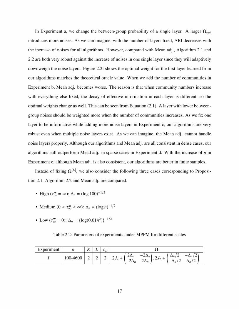
Instead of fixing Ω[L], we also consider the following three cases corresponding to Proposi-
tion 2.1. Algorithm 2.2 and Mean adj. are compared.
• High (τw∞ = ∞): ∆n = (log 100)−1/2
• Medium (0 < τw∞ < ∞): ∆n = (log n)−1/2
• Low (τw∞ = 0): ∆n = log(0.01n2)−1/2
Table 2.2: Parameters of experiments under MPPM for different scales
Experiment n K L cρ Ω
f 100-4600 2 2 2 2J2 +
(2∆n −2∆n−2∆n 2∆n
),2J2 +
(∆n/2 −∆n/2−∆n/2 ∆n/2
)
17
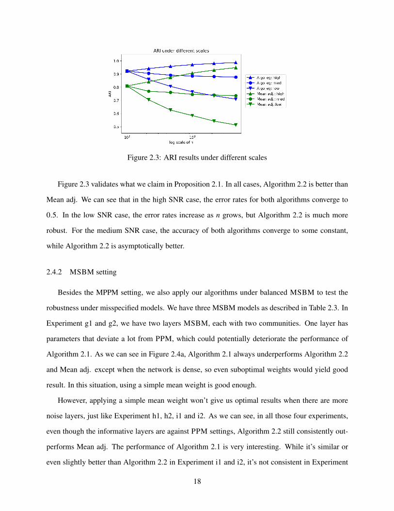
Figure 2.3: ARI results under different scales
Figure 2.3 validates what we claim in Proposition 2.1. In all cases, Algorithm 2.2 is better than
Mean adj. We can see that in the high SNR case, the error rates for both algorithms converge to
0.5. In the low SNR case, the error rates increase as n grows, but Algorithm 2.2 is much more
robust. For the medium SNR case, the accuracy of both algorithms converge to some constant,
while Algorithm 2.2 is asymptotically better.
2.4.2 MSBM setting
Besides the MPPM setting, we also apply our algorithms under balanced MSBM to test the
robustness under misspecified models. We have three MSBM models as described in Table 2.3. In
Experiment g1 and g2, we have two layers MSBM, each with two communities. One layer has
parameters that deviate a lot from PPM, which could potentially deteriorate the performance of
Algorithm 2.1. As we can see in Figure 2.4a, Algorithm 2.1 always underperforms Algorithm 2.2
and Mean adj. except when the network is dense, so even suboptimal weights would yield good
result. In this situation, using a simple mean weight is good enough.
However, applying a simple mean weight won’t give us optimal results when there are more
noise layers, just like Experiment h1, h2, i1 and i2. As we can see, in all those four experiments,
even though the informative layers are against PPM settings, Algorithm 2.2 still consistently out-
performs Mean adj. The performance of Algorithm 2.1 is very interesting. While it’s similar or
even slightly better than Algorithm 2.2 in Experiment i1 and i2, it’s not consistent in Experiment
18

Table 2.3: Parameters of experiments under MSBM
Experiment n K L cρ Ω
g1 6002 2
0.4-1.6(10 22 3
),
(3 22 3
)g2 600-1000 0.7
h1 6003 4
1.2-2.7 ©«9 2 22 2 22 2 9
ª®¬ ,©«2 2 22 4 22 2 2
ª®¬ ,2J3,2J3h2 600-1000 1.2
i1 6003 4
1.2-2.7 ©«8 2 22 6 22 2 4
ª®¬ ,2J3,2J3,2J3i2 600-1000 1.2
h1 and h2. The reason is that while Algorithm 2.2 is pretty robust when more noise layers present,
it can’t handle the case when SBM is too far away from PPM setting. This is straightforward
to see because Algorithm 2.1 relies heavily on PPM assumptions to derive the optimal weights.
Although we only prove the consistency of Algorithm 2.2 under MPPM, the simulation results
indicate that the theory may also hold for more general cases.
2.5 Real data example
We apply our algorithms to S&P 1500 data to see whether we could get extra information from
combining multilayer networks in practice. S&P 1500 index should be a good representative of
the US economy since it covers 90% of the market value of US stocks. We get the daily adjusted
close price of stocks from Yahoo! Finance, of which dates range from 2001-01-01 to 2019-06-30,
including 4663 trading days in total. We keep only stocks with less than 50 days’ missing data and
forward fill the price, which leaves us with 1020 stocks. According to the newest Global Industry
Classification Standard, there are in total of 11 sectors, which we treat as the hidden ground truth
that we hope to discover from stock prices. We remove sector ‘Communication Services’ because
of small sizes and sectors ‘Industrials’ and ‘Materials’ because of their similar performances during
economic cycles. The final dataset contains 770 stocks from 8 sectors.
We use the Pearson correlation of log returns between stocks to construct the network. The
19
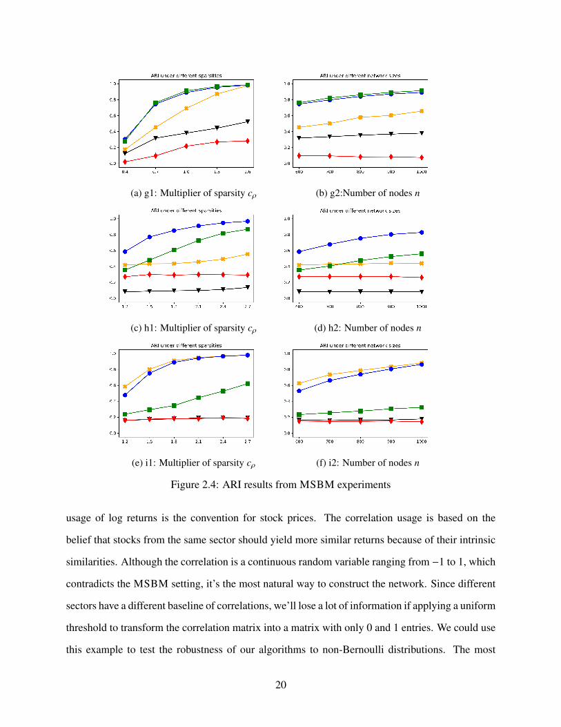
(a) g1: Multiplier of sparsity cρ (b) g2:Number of nodes n
(c) h1: Multiplier of sparsity cρ (d) h2: Number of nodes n
(e) i1: Multiplier of sparsity cρ (f) i2: Number of nodes n
Figure 2.4: ARI results from MSBM experiments
usage of log returns is the convention for stock prices. The correlation usage is based on the
belief that stocks from the same sector should yield more similar returns because of their intrinsic
similarities. Although the correlation is a continuous random variable ranging from −1 to 1, which
contradicts the MSBM setting, it’s the most natural way to construct the network. Since different
sectors have a different baseline of correlations, we’ll lose a lot of information if applying a uniform
threshold to transform the correlation matrix into a matrix with only 0 and 1 entries. We could use
this example to test the robustness of our algorithms to non-Bernoulli distributions. The most
20
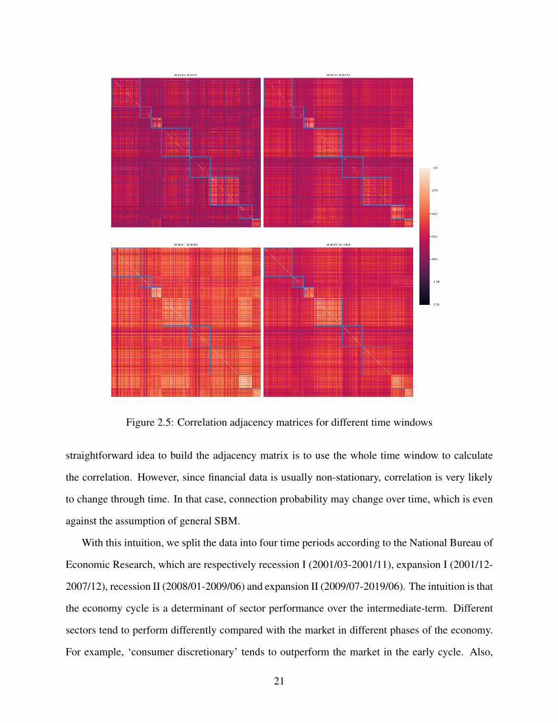
Figure 2.5: Correlation adjacency matrices for different time windows
straightforward idea to build the adjacency matrix is to use the whole time window to calculate
the correlation. However, since financial data is usually non-stationary, correlation is very likely
to change through time. In that case, connection probability may change over time, which is even
against the assumption of general SBM.
With this intuition, we split the data into four time periods according to the National Bureau of
Economic Research, which are respectively recession I (2001/03-2001/11), expansion I (2001/12-
2007/12), recession II (2008/01-2009/06) and expansion II (2009/07-2019/06). The intuition is that
the economy cycle is a determinant of sector performance over the intermediate-term. Different
sectors tend to perform differently compared with the market in different phases of the economy.
For example, ‘consumer discretionary’ tends to outperform the market in the early cycle. Also,
21
even within the same sector, correlation can vary a lot at different times, which could be handled
by our model. Taking a look at the correlation adjacency matrix in Figure 2.5, in which the box
represents different sectors. We could observe that the correlations vary during different time win-
dows. In the second recession period, we could observe an obviously higher correlation between or
within all sectors, which is exactly what we expect. Also, for the expansion period, there are larger
differences both within and between sectors. This demonstrates the necessity to use a multilayer
model in this example.
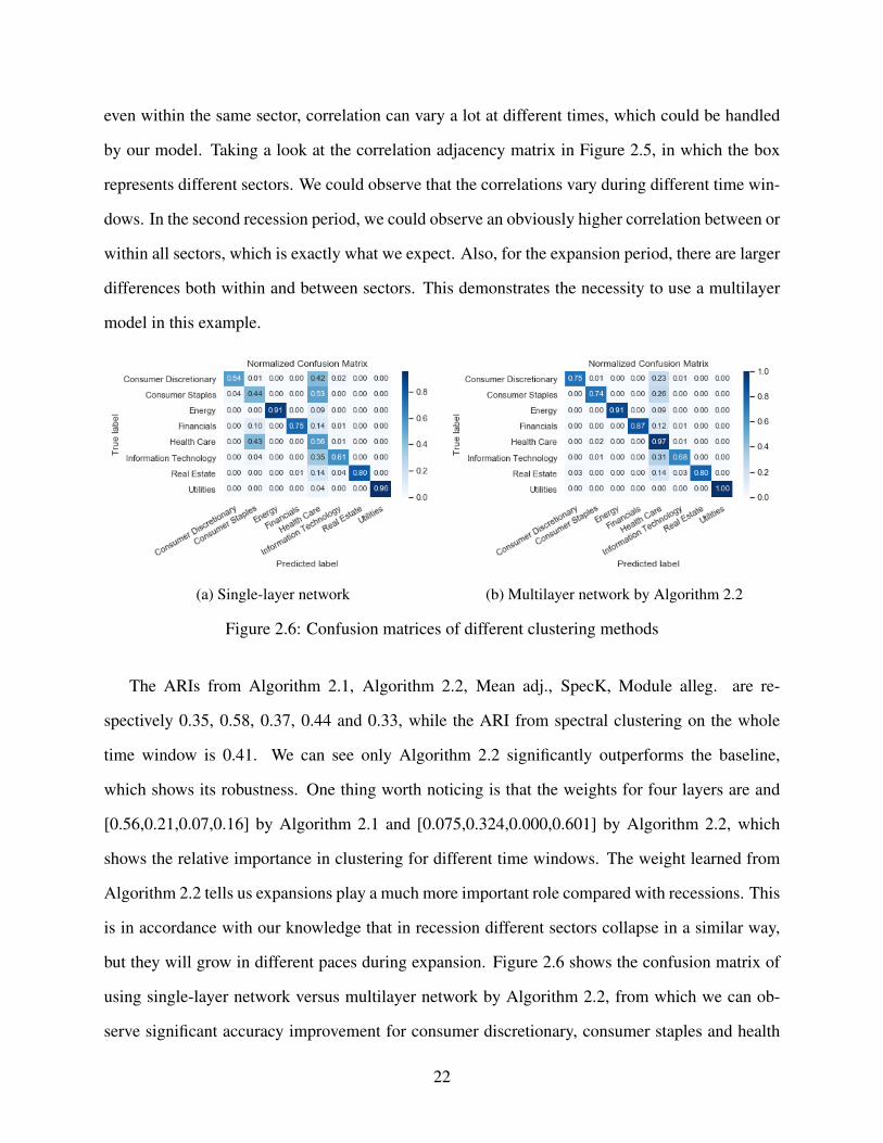
(a) Single-layer network (b) Multilayer network by Algorithm 2.2
Figure 2.6: Confusion matrices of different clustering methods
The ARIs from Algorithm 2.1, Algorithm 2.2, Mean adj., SpecK, Module alleg. are re-
spectively 0.35, 0.58, 0.37, 0.44 and 0.33, while the ARI from spectral clustering on the whole
time window is 0.41. We can see only Algorithm 2.2 significantly outperforms the baseline,
which shows its robustness. One thing worth noticing is that the weights for four layers are and
[0.56,0.21,0.07,0.16] by Algorithm 2.1 and [0.075,0.324,0.000,0.601] by Algorithm 2.2, which
shows the relative importance in clustering for different time windows. The weight learned from
Algorithm 2.2 tells us expansions play a much more important role compared with recessions. This
is in accordance with our knowledge that in recession different sectors collapse in a similar way,
but they will grow in different paces during expansion. Figure 2.6 shows the confusion matrix of
using single-layer network versus multilayer network by Algorithm 2.2, from which we can ob-
serve significant accuracy improvement for consumer discretionary, consumer staples and health
22

care sectors by using multilayer networks.
2.6 Discussion
Although we only prove Theorem 2.4 under balanced MPPM setting, we see the potential
of Algorithm 2.2 under more general models from both simulations and real data. For future re-
searches, one possibility is to extend the theoretical results to general SBM. Also, we only consider
assortative networks here. For disassortative cases, we may introduce negative weights.
We see a phase transition phenomenon in Proposition 2.3, and there are two possible research
directions that originated from here. One is whether below the threshold the problem is unsolvable
by spectral clustering. The other is whether the threshold we derive here is a threshold for all
algorithms or just for spectral clustering.
2.7 Proofs
The proofs are organized according to the order of the results in Section 2.3.
2.7.1 Proof of Proposition 2.1
To derive the error rate, we need to study the asymptotic distribution of eigenvectors first.
Similar to [129], we define the spectral embedding for general SBM. For a fixed positive integer
d ≤ n, we call the n× d matrix X = UAΛ1/2A the adjacency spectral embedding (ASE) of A into Rd .
We call X = ρ−1/2n UPΛ
1/2P and ν = UΩΛ
1/2Ω
respectively the probability spectral embedding (PSE)
and connectivity spectral embedding (CSE). Let µw denote the CSE of Ωw, then
µwµwT= Ωw =
L∑l=1
wlΩ(l) =
L∑l=1
wlν(l)ν(l)
T.
The entry of Ωw is Ωwi j =
∑Ll=1 wlν
(l)i·
Tν(l)j · = µ
wi·
T µwj ·. Similarly, define Pw = XwXwT .
Remark 2.1. When Ω is positive semi-definite, which is true for assortative SBM since it’s a Gram
matrix. By taking d = K , we have Ω = ννT . Since P is an augmentation of Ω, we know ΛP = ΛΩ
23
and rows of UP are just replications of rows of UΩ. We will still keep d instead of K in later
statements to avoid the confusion of columns and rows.
Remark 2.2. The PPM assumes homogeneous probability across different communities. In this
case, we know the exact eigenvalues are λ1(Ω) = Ωin + (K − 1)Ωout and λ2(Ω) = · · · = λd(Ω) =
Ωin −Ωout . When Ωin > Ωout , Ω is full rank. The orthogonal eigenvectors are chosen as
UΩ =
K−1/2 −(K − 1)/K1/2 0 · · · 0
K−1/2 K(K − 1)−1/2 −(K − 2)/(K − 1)1/2 · · · 0...
......
. . ....
K−1/2 K(K − 1)−1/2 (K − 1)(K − 2)−1/2 · · · 2−1/2
∈ RK×d,
then
ν =
(λ1/K)1/2 −λ2(K − 1)/K1/2 0 · · · 0
(λ1/K)1/2 [λ2/K(K − 1)]1/2 −λ3(K − 2)/(K − 1)1/2 · · · 0...
......
. . ....
(λ1/K)1/2 [λ2/K(K − 1)]1/2 [λ3/(K − 1)(K − 2)]1/2 · · · (λd/2)1/2
∈ RK×d .
In [129], the eigenvector distribution for SBM has been discussed thoroughly, the question
remains to be whether the eigenvector distribution of WAM still asymptotically follows a multi-
variate normal distribution. This result will be validated and expanded here, which is organized
as follows. First, we introduce a direct consequence of Corollary 2.3 in [129] and prove a parallel
theorem for WAM. Then, we’ll prove a theorem when the connection of the random graph changes
with n rather than fixed as usual. We will only focus on the case when ρn → 0 because ρn = 1 is
trivial in terms of the clustering error rate.
Theorem 2.5 (ASE convergence). Let A[L] ∼ MSBM(Ω[L],c, ρn). For any fixed w ∈ WL , consider
the spectral embedding of Aw. There exists an orthogonal matrix Wn ∈ Rd×d and a matrix Rn ∈
n × d such that
XwWn − ρ1/2n Xw = ρ
−1/2n (Aw − Pw)Xw(XwT Xw)−1 + Rn.
24

Also, ‖Rn‖ = O((nρn)−1/2). Let θ l = E[X
(l)1· ] for l ∈ [L] and ∆w = E[Xw
1·Xw1·
T ]. If Condition 2.1
holds, then there exists a sequence of orthogonal matrices Wn ∈ Rd×d satisfying
‖ XwWn − ρ1/2n Xw‖2F
a.s.−−→ trace
[∆−1w E
Xw
1·Xw1·
T
(L∑
l=1w2
l X (l)1·Tθ l
)∆−1w
].
Theorem 2.6 (WAM eigenvector distribution). Let A[L] ∼ MSBM(Ω[L],c, ρn), then for any fixed
w ∈ WL , consider the spectral embedding of Aw. If Condition 2.1 holds, then for any fixed index
i, given ci = k, there exists a sequence of orthogonal matrices Wn satisfying
n1/2(Wn Xwi· − ρ
1/2n Xw
i· )d−→ N(0,Σk),
where Σk = ∆−1w E[X
w1·X
w1·
T ∑Ll=1 w
2l ν(l)k ·
TX (l)1· ]∆
−1w .
Corollary 2.7 (SBM eigenvector distribution). Let A ∼ SBM(Ω,c, ρn), if Condition 2.1 holds, then
there exists a sequence of orthogonal matrices Wn such that for any fixed index i that Xi· = νk ·,
n1/2(Wn Xi· − ρ1/2n Xi·)
d−→ N(0,Σk),
where Σk = ∆−1E[(νT
k ·X1·)X1·XT1·]∆
−1 = ∆−1(∑K
i=1 πiΩikνi·νTi· )∆
−1 and∆ = E[X1·XT1·] =
∑Kk=1 πkνk ·ν
Tk ·.
Corollary 2.7 is straightforward from Theorem 2.6 since a single layer SBM is just a special
case of WAM. It is exactly the same as what we could derive from Corollary 2.3 in [129] since
all assortative SBM can be expressed in the form of the random dot product graph. The only
difference between WAM and SBM is the variance. Since WAM changes the variance rather than
the mean of the edge weight, this consequence should be expected.
From Theorem 2.6, we can see as long as νk are distinct, the asymptotic eigenvector distribution
will be different, which makes the clustering problem relatively easy. To provide more insights,
we consider the case when the mean connection probabilities of different communities converge
to the same value, i.e., the connectivity matrix Ω is allowed to change with n but with a finite limit
Ω∞, whose elements are all the same. By Remark 2.2, we see the first eigenvector is determined
25

by the degree and doesn’t contribute to community detection, so we consider the ‘effective’ CSE,
which is the sub-matrix corresponding to λ2(Ωw) until λd(Ω
w). Since λ2(Ωw) = · · · = λd(Ω
w), we
could define the ‘effective’ CSE as
µw =√λw
2
−(K − 1)/K1/2 0 · · · 0
K(K − 1)−1/2 −(K − 2)/(K − 1)1/2 · · · 0...
.... . .
...
K(K − 1)−1/2 (K − 1)(K − 2)−1/2 · · · 2−1/2
=[µ1, · · · , µK]
T =
√λw
2 [u1, · · · ,uK]T ∈ RK×(d−1),
which is just a constant matrix multiplied by√λw
2 . We can see that for fixed K , u1, · · · ,uK are just
fixed constant vectors.
Notice that
∆w =1K
K∑k=1
µwk ·µ
wk ·
T=
1KµwT µw =
1K
D((λ1(Ωw), · · · , λd(Ω
w))T )
and
ν(l)k ·
Tν(l)m· = Ω
(l)km =
Ω(l)in if k = m,
Ω(l)out if k , m.
So
E[Xw1·X
w1·
TL∑
l=1w2
l ν(l)k ·
TX (l)1· ] =
1K
K∑m=1
µwm·µ
wm·
TL∑
l=1w2
l Ω(l)km
=Ωw2
out
K
K∑m=1
µwm·µ
wm·
T+Ωw2
in −Ωw2out
Kµw
k ·µwk ·
T=Ωw2
out
KµwT µw +
Ωw2
in −Ωw2out
Kµw
k ·µwk ·
T
=Ωw2
out
KD((λ1(Ω
w), · · · , λd(Ωw))T ) +
Ωw2
in −Ωw2out
Kµw
k ·µwk ·
T .
26

Then it’s straight forward to see
Σk =∆−1w
[Ωw2
out
KD((λ1(Ω
w), · · · , λd(Ωw))T ) +
Ωw2
in −Ωw2out
Kµw
k ·µwk ·
T
]∆−1w
=KΩw2
out D((1/λ1(Ωw), · · · ,1/λd(Ω
w))T ) +Ωw2
in −Ωw2out
K∆−1w µw
k ·µwk ·
T∆−1w .
We define Σk to be the sub-matrix of Σk corresponding to µw. Also, we could define the limit
‘effective’ covariance matrix
Σ =Ωw2
in + (K − 1)Ωw2out
Ωwin −Ω
wout
Id−1 ≡ σ2wId−1,
then it’s easy to see that Σk Σ−1 p−→ I. Here we require that there ∃w s.t. σw , ∞. This is equivalent
to ∃l ∈ [L] s.t. Ω(l)in , Ω(l)out , otherwise the problem is undetectable.
Based on Theorem 2.6, we could have the following theorem by the Slutsky’s theorem.
Theorem 2.8 (WAM with varied mean). Let A[L]n ∼ MSBM(Ω[L]n ,c, ρn). For l ∈ [L], assume
limn→∞Ω(l)n = Ω
(l)∞ ∈ R
K×K , whose entries are all the same. Also, there ∃l ∈ [L] s.t. Ω(l)in , Ω(l)out .
For any fixed w ∈ WL , if Condition 2.1 holds, there exists a sequence of orthogonal matrices Wn
such that for any fixed index i that ci = k,
σ−1w n1/2(Wn Xw
i,2:d − ρ1/2n Xw
i,2:d)d−→ N(0, Id−1).
Under the setting of Theorem 2.8, the asymptotic variance for different classes are all the same,
which reduces the clustering problem from QDA to LDA. Also, the problem becomes non-trivial
since the asymptotic means are all the same, so the error rate may not converge to 0 as before. We
consider the probability of classifying a node to group k for k ≥ 2 when it’s from group 1 if only
considering a two-class classification problem. The asymptotic distribution for ci = k,
(nρnλw2 )
1/2
σwXi,2:d/(ρnλ
w2 )
1/2 − ukd−→ N(0, Id−1).
27

Since we use UA for spectral clustering, here we focus on Xi,2:d/(ρnλw2 )
1/2, whose density function
under group k is
fk(x) =(nρnλ
w2 )
1/2
(2π)(d−1)/2σwexp
−
nρnλw2
2σ2w(x − uk)
T (x − uk)
.
The probability of misclassifying k-th class to 1st class is P( fk ≥ f1 |1) =∫x∈Rk1
f1(x)dx, where
Rk1 =x ∈ Rd−1 | (x − 1
2 (uk + u1))T (uk − u1) ≥ 0
is the region that the likelihood of group k is
larger than group 1.
We can see that the region is a constant scale area and has nothing to do with Ωw and n.
Since the centers u1, · · · ,uk are all fixed, the error rate only depends on the SNR, which is
(nρnλw2 )
1/2/σw = 2K1/2τwn . When K fixed, the error rate is monotonic decreasing with τw
n and
the conclusion in Proposition 2.1 can be seen. In general, we can always maximize τwn to mini-
mize the asymptotic error. Specifically, when Ωw is fixed and Ωwin , Ω
wout , the limiting error rate
is always 0 since uk are distinct, although we can still minimize finite sample error rate. When
Ωwin − Ω
wout = Θ((nρn)
−1/2), which is case 3, we can minimize the error rate even in the asymptotic
sense.
A. Proof of Theorem 2.5
Proof. We need to bound ‖Aw − Pw‖ like Proposition 7 in [97]. We show a stronger result, which
can be seen directly from Theorem 5.2 of [91]. Since we don’t need to prove the theorem for the
laplacian matrix, we only need ρn of order log n/n instead of log4 n/n.
Lemma 2.9. For any constant c,r > 0, there exists constant C(c,r) > 0 independent of n and
w such that the following holds. If ‖Pw‖1 > c log n, then with probability at least 1 − n−r , the
following hold
‖Aw − Pw‖ ≤ C√‖Pw‖1.
Following the same proof procedure of Theorem A.5 in [128], we can prove the following
lemma. Since all procedures are the same once Lemma 2.9 is established, we’ll omit the proof of
28

Lemma 2.10.
Lemma 2.10. Under the same assumption in Lemma 2.9, there exists an orthogonal matrix Wn
such that for sufficiently large n,
‖ Xw − ρ1/2n XwWn‖ = ‖(Aw − Pw)UPw S−1/2
Pw ‖F +O(d‖Pw‖21λd(Pw)−5/2
)with high probability.
To verify Theorem 2.5, all steps are the same as Theorem 2.1 in [129], except for the calculation
of E[(Aw − Pw)2], so we only show that part here. Since
E
[∑k
(Awik − Pw
ik)(Awk j − Pw
k j)
]=
0 if i , j,∑
k,i∑L
l=1 w2l P(l)k j (1 − P(l)k j ) if i = j,
so
n−2ρ−1n XwTE
[(Aw − Pw)2
]Xw = n−2ρ−1
n
n∑i=1
Xwi· Xw
i·T∑k,i
L∑l=1
w2l P(l)ki (1 − P(l)ki )
=n−2n∑
i=1Xw
i· Xwi·
T∑k,i
L∑l=1
w2l X
(l)i·
TX (l)k · − ρn(X
(l)i·
TX (l)k · )
2
When ρn → 0, the above term converges to
E[Xw1·X
w1·
T(∑
l
w2l X (l)1
Tθ l)].
29

B. Proof of Theorem 2.6
Proof. The proof is similar to the proof of Theorem 2.2 in [129] except for the variance calculation.
For any fixed index i we have
√n(Wn Xw
i· − ρ1/2n Xw
i· ) =√
nρ−1/2n (XwT Xw)−1
∑j,i
(Ai j − Pi j)Xwj · + o(1)
=(n−1XwT Xw)−1∑i, j
(Awi j − ρn
∑l wl X
(l)i·
TX (l)j · )
√nρn
Xwj · + o(1)
Given Xwi· = µk ,
∑i, j(Aw
i j − ρn∑
l wl X(l)i·
TX (l)j · )X
wj · is a sum of i.i.d. mean zero random variables.
The conditional variance is calculated as
E[(Awi j − ρn
∑l
wlν(l)k ·
TX (l)j · )
2Xwj · X
wj ·
T]
=Em[E[(Awi j − ρn
∑l
wlν(l)k ·
TX (l)j · )
2Xwj · X
wj ·
T|Xw
j · = µm]]
=Em[µmµTmE[(A
wi j − ρn
∑l
wlν(l)k ·
TX (l)j · )
2 |Xwj · = µm]]
=ρnEm[µmµTm
L∑l=1
w2l ν(l)k ·
Tν(l)m·(1 − ρnν
(l)k ·
Tν(l)m·)].
This yields
∑i, j
(Awi j − ρn
∑l wl X
(l)i·
TX (l)j · )
√nρn
Xwj ·
d−→ N(0,E[Xw
1·Xw1·
TL∑
l=1w2
l ν(l)k ·
TX (l)1 (1 − ρnν
(l)k ·
TX (l)1 )]).
Since n−1XwT Xw a.s.−−→ ∆w as n→∞, by Slutsky’s theorem, when ρn → 0,
√n(Wn Xw
i· − ρ1/2n Xw
i· )d−→ N(0,∆−1
w E[Xw1·X
w1·
TL∑
l=1w2
l ν(l)k ·
TX (l)1· ]∆
−1w ).
30

2.7.2 Proof of Proposition 2.3
Results in this subsection will mostly be based on Proposition 2 in [15] with some slight mod-
ifications. By studying the asymptotic behavior of eigenvalue gap λwK/λ
wK+1, we will see clearly
its connection with SNR τwn , which results in Theorem 2.4. Since general SBM doesn’t have an
explicit solution for eigenvalues, we consider only balanced PPM here, whose eigenvalues have an
explicit form.
We first make a decomposition as in [15] and state the spectrum property as follows.
Proposition 2.11 (WAM decomposition). Suppose Aw is the WAM generated from a balanced
MPPM. Consider the scaled matrix Aw = γ(n)Aw, where γ(n) = K/nρn(Ωwin − Ω
wout). We
decompose Aw into two parts
Aw = Aw + Aw,
where Aw = γ(n)Pw is the expectation of Aw and Aw is a random matrix with zero mean random
entries. The spectrum property of Aw and Aw is summarized as follows.
1. Aw is of rank K and the 2nd to Kth largest eigenvalues all converge to 1.
2. The spectrum bound of Aw is 1/τwn , the reciprocal of SNR.
According to [23], the scale of τwn determines the behavior of the 2nd to Kth eigenvalues, which
is crucial for determining the spectrum of Aw. The property is summarized as follows.
Proposition 2.12 (WAM spectrum). Based on the decomposition in Proposition 2.11, τw∞ deter-
mines the asymptotic behavior of the spectrum of Aw as follows.
1. If τw∞ = ∞, the asymptotic spectrum of Aw and Aw are the same since the noises degenerate.
2. If τw∞ = 0, the asymptotic spectrum of Aw and Aw are the same since the noises dominate.
3. If τw∞ is a finite constant, the signals and noises are in the same scale. Specifically,
(a) If τw∞ > 1/2, the 2nd to Kth eigenvalue of Aw converges to 1 + (4τw
∞)−2.
31

(b) If τw∞ ≤ 1/2, the 2nd to Kth eigenvalue of Aw converges to τw
∞−1.
We can see that τw∞ is monotonic with the eigenvalue gap λw
K/λwK+1. A larger τw
∞ leads to a larger
gap, except when τw∞ ≤ 1/2, in which case the noises still dominate signals. When τw
∞ > 1/2, the
limit of eigenvalue gap converges to (4τw∞)−1 + τw
∞, which is monotonic increasing with τw∞. Thus,
we can maximize the eigenvalue gap to maximize τwn asymptotically. This shows Theorem 2.4.
The proofs of Proposition 2.11 and 2.12 are mainly based on the semicircle law of Aw [15],
and Theorem 2.1 in [23], which shows the spectrum property of the perturbations of large random
matrices.
A. Proof of Proposition 2.11
Proof. By some algebra, it’s easy to show Aw is similar to some matrix with only K × K non-zero
entries, whose eigenvalues are the same as the following K × K matrix
Yn =K
n(Ωwin −Ω
wout)
D((n1, · · · ,nK)T )Ωw
=1
Ωwin −Ω
woutΩ
w +1
Ωwin −Ω
wout
D((1 − Kn1n−1, · · · ,1 − KnKn−1)T )Ωw.
By decomposing Yn into two parts, we see that the 2nd to Kth eigenvalues of the first part is
exactly 1. For the second part, since 1 − Knin−1 = Θ(n−1/2) by CLT, as long as Ωwin − Ω
wout =
ω(n−1/2), the second matrix converges to 0 elementwisely, so do all the eigenvalues. By Weyl’s
eigenvalue interlacing inequalities, the 2nd to Kth eigenvalues of Yn converge to 1 as well.
Intuitively, the bound of Aw represents the magnitude of noises, which we hope to be as small
as possible. To obtain the bound, we consider the following scaling and decomposition. Let swi =
∑L
l=1 w2l∑
j P(l)i j (1 − P(l)i j )1/2 be the empirical standard deviation of node i and sw = nρn(Ω
w2
in +
(K − 1)Ωw2out)/K
1/2 be the population standard deviation. Then
Aw − Pw
sw =
[Aw
i j − Pwi j
swi
]n×n
+
[(Aw
i j − Pwi j )(
1sw
i−
1sw )
]n×n
.
32
The first part is a generalized Wigner matrix, so its eigenvalues follow local semicircle law accord-
ing to [54]. We claim that the spectrum bound of the second matrix converges to 0 asymptotically.
Then by Weyl’s inequality, we know the asymptotic spectrum distribution of (Aw − Pw)/sw is not
affected by the deformation, so it follows local semicircle law as well.
To validate the claim, we show a more general spectrum bound using the conclusion from [21].
Let dw = maxi∑L
l=1 w2l∑
j P(l)i j , Hw = d−1/2w (Aw − Pw), q = [nρnK−1Ωw2
in + (K − 1)Ωw2out]
1/2
and κ = (Ωw2
in /Ωwout)
2. It’s easy to verify that dw ≥ q2, |Hwi j | ≤ d−1/2
w ≤ 1/q and EHwi j
2 ≤∑Ll=1 w
2l P(l)i j /dw ≤ 1, then Hw satisfies the following assumption.
Condition 2.3. Let H be a symmetric random matrix whose upper triangular entries (Hi j)1≤i≤ j≤n
are independent mean-zero random variables. Moreover, suppose that there exist q > 0 and κ ≥ 1
such that
maxi
∑j
E[H2i j] ≤ 1, max
iE[H2
i j] ≤κ
n, max
i,j|Hi j | ≤
1q
a.s.
Directly applying Theorem 2.6 in [21], we have the following theorem.
Theorem 2.13. Assume Assumption 2.3 is satisfied by Hw, then for 2 ∨ q ≤ n1/13κ−1/12,
E‖Hw‖ ≤ 2 + Cη
(1 ∨ log η)1/2, with η =
(log n)1/2
q,
for some universal constant C > 0. In particular,
E‖Hw‖ ≤ 2 + C(log n)1/2
q.
Theorem 2.13 shows that with high probability, ‖Hw‖ ≤ 2 + o(1) as long as q2 log n and
κ n12/13. By Theorem 2.2 of [81] and Corollary 1.4 of [22], we know this bound is actually
sharp. Since (swi sw)−1(sw
i − sw)d1/2w = Θ(n−1/2), we know from Theorem 2.13 that the spectrum
bound of the second matrix is Θ(n−1/2), which validates the claim.
33

From above discussion, we know immediately that ‖ Aw‖ is bounded by
2swγ(n) = 2(
Knρn
)1/2 Ωw2
in + (K − 1)Ωw2out
1/2
Ωwin −Ω
wout
=1τw
n.
When τw∞ is finite, the semi-circle law holds for Aw with bound 1/τw
∞.
B. Proof of Proposition 2.12
Proof. Now we know τw∞ plays a critical role in determining the asymptotic spectrum distribution
of Aw. When τw∞ = 0, the 2nd to Kth eigenvalues of Aw will be dominated by unbounded noises.
When τw∞ = ∞, the asymptotic behavior of Aw will be exactly the same as Aw. When 0 < τw
∞ < ∞,
[23] provides us with the necessary tool to determine the spectrum distribution of Aw, which is the
summation of a low-rank matrix Aw and a noise matrix Aw whose eigenvalues are both constant
scale.
For a symmetric matrix Xn ∈ Rn×n with ordered eigenvalues λ1(Xn) ≥ · · · ≥ λn(Xn). Let fXn
be the empirical eigenvalue distribution, which is
fXn =1n
n∑j=1
δλj (Xn).
If fXn converges almost surely weakly, as n → ∞, to a non-random compactly supported proba-
bility measure, we let fX∞ denote the limit. Let aX∞ and bX∞ be the infimum and supremum of the
support of fX∞ , then the smallest and largest eigenvalue of Xn converge almost surely to aX∞ and
bX∞ .
Since Aw ∈ Rn×n is a positive semi-definite matrix with rank K , and limn→∞ λi(Aw) = 1 for
i = 2, · · · ,K . Applying Theorem 2.1 and Remark 2.15 in [23], we have the following theorem.
Theorem 2.14. The extreme eigenvalues of Aw exhibit the following behavior as n→∞. We have
34

that for each 1 ≤ i ≤ K,
λi(Aw)a.s.−−→
G−1
fX(1) if G fX∞ (b
+) < 1,
b otherwise,(2.2)
while for each fixed i > K , λi(Aw)a.s.−−→ b. Here,
G fX (z) =∫
1z − t
dfX(t) for z < supp fX,
is the Cauchy transform of fX , G−1fX(·) is its functional inverse so that 1/±∞ stands for 0.
By semicircle law [15], fAw∞(t) = 2π−1τw
∞2(1/τw
∞2 − t2)+
1/2, then it’s easy to verify that
G fX (z) =
τw∞
22z − 2(z2 − 1/τw∞
2)1/2 if z > 1/τw∞,
τw∞
22z + 2(z2 − 1/τw∞
2)1/2 if z < −1/τw∞,
G fX (±1/τw∞) = ±1/2τw
∞ and G−1fX(1/x) = (4xτw
∞2)−1 + x for x , 0. Thus, for 2 ≤ i ≤ K ,
λi(Aw)a.s.−−→
1 + (4τw
∞2)−1, if τw
∞ > 1/2,
1/τw∞, otherwise.
35
Chapter 3: Pairwise Covariate-Adjusted Block Model
3.1 Introduction
In the real world, the connection of nodes may depend on not only community structure but also
on some nodal information. For example, in an ecological network, the predator-prey link between
species may depend on their prey types as well as their habits, body sizes and living environment.
Incorporating nodal information into the network model should help us recover a more accurate
community structure.
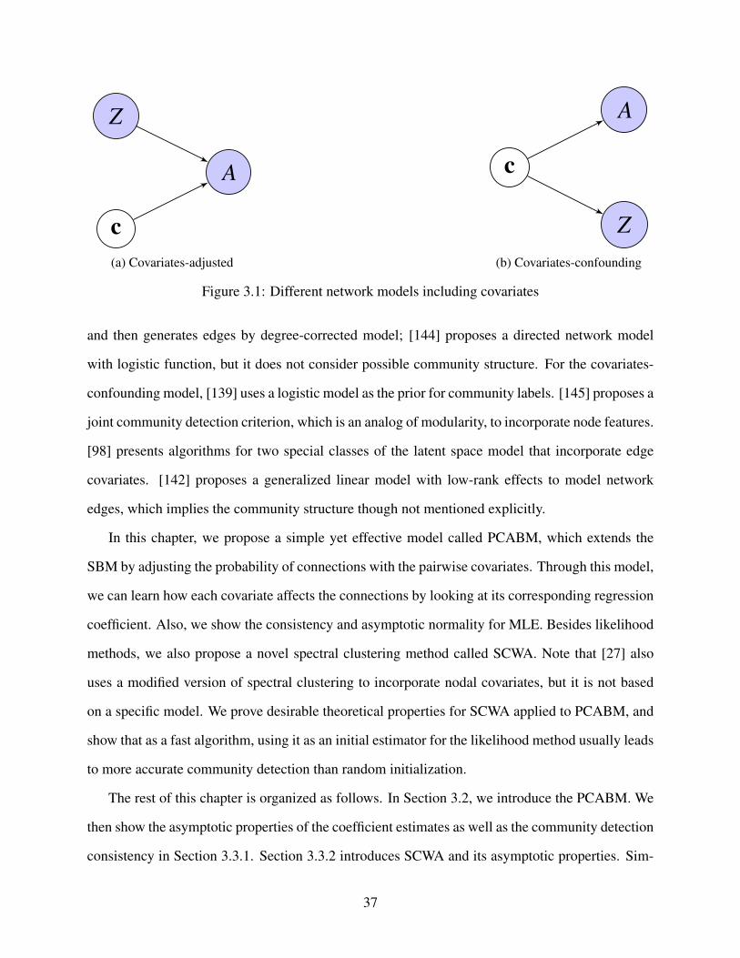
Depending on the relationship between communities and covariates, there are in general two
classes of models as shown in Figure 3.1: covariates-adjusted and covariates-confounding. c, X
and A respectively stands for latent community label, nodal information and adjacency matrix.
In Figure 3.1a, the latent community and the covariates jointly determine the network structure.
One typical example of this model is the friendship network between students. Students become
friends for various reasons: they are in the same class; they have the same hobbies; they are of the
same ethnic group. Without adjusting those covariates, it is hard to believe A represents any single
community membership. We will analyze one such example in detail in Section 3.5. On the other
hand, covariates sometimes carry the same community information as the adjacency matrix, which
is shown in Figure 3.1b. The name ‘confounding’ comes from graph model [68]. Citation network
is a perfect example of this model [127]. When the research topic is treated as the community label
for each article, the citation links would largely depend on the research topics of the article pair.
Meanwhile, the distribution of the keywords is also likely to be driven by the specific topic the
article is about.
Most researchers modify SBM in the above two ways to incorporate covariates’ information.
For the covariates-adjusted model, [111] uses covariates to construct the prior for community label
36
Z
A
c(a) Covariates-adjusted
c
A
Z(b) Covariates-confounding
Figure 3.1: Different network models including covariates
and then generates edges by degree-corrected model; [144] proposes a directed network model
with logistic function, but it does not consider possible community structure. For the covariates-
confounding model, [139] uses a logistic model as the prior for community labels. [145] proposes a
joint community detection criterion, which is an analog of modularity, to incorporate node features.
[98] presents algorithms for two special classes of the latent space model that incorporate edge
covariates. [142] proposes a generalized linear model with low-rank effects to model network
edges, which implies the community structure though not mentioned explicitly.
In this chapter, we propose a simple yet effective model called PCABM, which extends the
SBM by adjusting the probability of connections with the pairwise covariates. Through this model,
we can learn how each covariate affects the connections by looking at its corresponding regression
coefficient. Also, we show the consistency and asymptotic normality for MLE. Besides likelihood
methods, we also propose a novel spectral clustering method called SCWA. Note that [27] also
uses a modified version of spectral clustering to incorporate nodal covariates, but it is not based
on a specific model. We prove desirable theoretical properties for SCWA applied to PCABM, and
show that as a fast algorithm, using it as an initial estimator for the likelihood method usually leads
to more accurate community detection than random initialization.
The rest of this chapter is organized as follows. In Section 3.2, we introduce the PCABM. We
then show the asymptotic properties of the coefficient estimates as well as the community detection
consistency in Section 3.3.1. Section 3.3.2 introduces SCWA and its asymptotic properties. Sim-
37

ulations and applications on real networks will be discussed in Section 3.4 and 3.5. We conclude
this chapter with a short discussion in Section 3.6. All proofs are relegated to Section 3.7.
3.2 PCABM setup
Upon classical SBM, we assume in addition to A, we have additionally observed a pairwise p-
dimensional vector zi j between node i and j. Denote the collection of the pairwise covariate among
nodes as Z = [zTi j] ∈ R
n2×p. Define γ as a fixed common coefficient vector for all node pairs (i, j)
with the true value denoted by γ0. For i < j, conditioned on c, Z,γ0,B, Ai j’s are independent and
Ai j ∼ Poisson(λi j), λi j = Bcicj ezTijγ
0.
In this thesis, we only consider sparse networks, which means λi j is far less than 1. For simplicity,
we assume λi j < 1/2. The specific term ezTijγ0
is introduced here to adjust the SBM with the
pairwise covariates. ϕn is no longer the expected degree as in [147], but we can still use it to
measure the rate of ρn. For theoretical purposes, we need the following conditions on Z and γ0.
Condition 3.1. zi j, i < j are i.i.d. and zi j = z ji.
Condition 3.2. zi j, i < j are uniformly bounded, i.e., for ∀i < j, ‖zi j ‖∞ ≤ ζ , where ζ > 0 is
some constant.
Remark 3.1. The bounded support condition for zi j is introduced to simply our proofs. It could
be relaxed to allow the upper bound grow slowly with network size n.
By Condition 3.2, we know that ezTijγ0
is also uniformly bounded. We define the bound as βl ≤
ezTijγ0≤ βu. Thus, the following expectations exist: θ(γ0) ≡ EezTijγ
0∈ R+, µ(γ0) ≡ Ezi je
zTijγ0∈ Rp,
and Σ(γ0) ≡ Ezi jzTi je
zTijγ0∈ Rp×p.
Condition 3.3. Σ(γ0) − θ(γ0)−1µ(γ0)⊗2 is positive definite.
Remark 3.2. Condition 3.3 is imposed to ensure that γ0 is the unique solution to maximize the
likelihood in the population version. Consider the function g(γ) = θ(γ)Σ(γ) − µ(γ)⊗2. If γ0 = 0,
38

we have g(0) = E[z⊗2] − E[z]⊗2 = cov(z). To avoid multicollinearity, it’s natural for us to require
cov(z) to be positive definite. Similarly, we require g(γ0) to be positive definite at the true value
γ0.
Define
nk(e) ≡n∑
i=11ei=k, Okl(e) ≡
∑i j
Ai j1ei=k,ej=l, Ekl(e,γ) ≡∑i, j
ezTijγ1ei=k,ej=l =∑
(i,j)∈se(k,l)
ezTijγ,
where se(k, l) = (i, j)|ei = k, e j = l, i , j. Under assignment e, nk(e) represents the number of
nodes in community k. For k , l, Okl is the total number of edges between communities k and l;
for k = l, Okk is twice of the number of edges within community k. Ekl is the summation of all
pair-level factors. We can write the log-likelihood function as
logL(e,γ,B,π |A, Z) ∝∑
k
nk(e) log πk +12
∑kl
Okl(e) log Bkl −12
∑kl
Bkl Ekl(e,γ) +∑i< j
Ai jzTi jγ.
For fixed e and γ, the MLE of π and B is πk(e) = nk(e)/n and Bkl(e) = Okl(e)/Ekl(e,γ).
Plugging B(e), π(e) into the original log-likelihood and discarding the constant terms, we have
logL(e,γ, B, π |A, Z) ∝12
∑kl
Okl(e) logOkl(e)
Ekl(e,γ)+
∑i< j
Ai jzTi jγ +
∑k
nk(e) lognk(e)
n. (3.1)
Out target is to maximize (3.1) w.r.t. e and γ. To achieve that, we apply a two-step procedure here,
which means we estimate γ0 and c sequentially. The theoretical properties for the MLE γ and c
will be demonstrated in the following section.
3.3 Theory and algorithms for PCABM
In this section, we will introduce two approaches for PCABM estimation. One is likelihood
method in Section 3.3.1, and the other is a modified spectral clustering method in Section 3.3.2.
While the former is the canonical analysis for a new model, the latter is a more efficient approach.
39

3.3.1 Likelihood method
The likelihood theory will be divided into three parts. First, we investigate the property of MLE
γ(e) under some random community assignment e. We derive the consistency and asymptotic
normality of γ(e) under some mild conditions of e. Second, we demonstrate that under a large
class of criteria Q, given γ(e) is consistent, the consistency of c(e) is guaranteed under PCABM.
At last, we show that under our likelihood criterion, c is consistent under any γ, even if it’s not
consistent, which could potentially save time by skipping the γ estimation step.
A. Consistency of γ
Consider the terms in (3.1) only containing γ, which is
`e(γ) ≡∑i< j
Ai jzTi jγ −
12
∑kl
Okl(e) log Ekl(e,γ).
Define γ(e) ≡ arg maxγ `e(γ) to be the MLE. When there is no need to emphasize, we will simply
omit e. To derive the asymptotic property for γ, the following regularity condition regarding the
community assignment e is assumed.
Condition 3.4 (non-degeneracy). For any k ∈ [K], κ1 ≤ |nk(e)/n| ≤ κ2, where 0 < κ1 ≤ κ2 < 1
are some positive constants.
Condition 3.4 is very mild and natural since we know the size of each community is approxi-
mately a constant proportion of the total number of nodes under the true model. The consistency
of γ is guaranteed by the following theorem.
Theorem 3.1. Under PCABM, assume Condition 3.1, 3.3 and 3.4 hold. As n→∞, if Nnρn →∞,
γ(e)p−→ γ0.
This theorem saves us from tedious estimations of γ0 and c iteratively. It shows that we can
get a consistent estimate of γ0 under any community assignment e with mild conditions. With
Theorem 3.1, we no longer need a good initial estimate of c to guarantee the consistency of γ. We
40
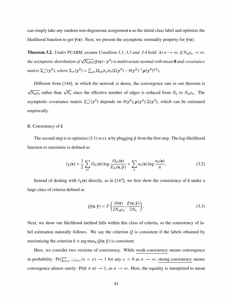
can simply take any random non-degenerate assignment e as the initial class label and optimize the
likelihood function to get γ(e). Next, we present the asymptotic normality property for γ(e).
Theorem 3.2. Under PCABM, assume Condition 3.1, 3.3 and 3.4 hold. As n→∞, if Nnρn →∞,
the asymptotic distribution of√
Nnρn(γ(e)−γ0) is multivariate normal with mean 0 and covariance
matrix Σ−1∞ (γ
0), where Σ∞(γ0) =∑
abΩabπaπb(Σ(γ0) − θ(γ0)−1µ(γ0)⊗2).
Different from [144], in which the network is dense, the convergence rate in our theorem is√
Nnρn rather than√
Nn since the effective number of edges is reduced from Nn to Nnρn. The
asymptotic covariance matrix Σ−1∞ (γ
0) depends on θ(γ0), µ(γ0),Σ(γ0), which can be estimated
empirically.
B. Consistency of c
The second step is to optimize (3.1) w.r.t. e by plugging γ from the first step. The log-likelihood
function to maximize is defined as
`γ(e) =12
∑kl
Okl(e) logOkl(e)
Ekl(e, γ)+
∑k
nk(e) lognk(e)
n. (3.2)
Instead of dealing with `γ(e) directly, as in [147], we first show the consistency of c under a
large class of criteria defined as
Q(e, γ) = F(
O(e)2Nnρn
,E(e, γ)
2Nn
). (3.3)
Next, we show our likelihood method falls within this class of criteria, so the consistency of la-
bel estimation naturally follows. We say the criterion Q is consistent if the labels obtained by
maximizing the criterion c ≡ arg maxe Q(e, γ) is consistent.
Here, we consider two versions of consistency. While weak consistency means convergence
in probability: Pr(∑n
i=1 1ci,ci/n < ε) → 1 for any ε > 0 as n → ∞, strong consistency means
convergence almost surely: Pr(c , c) → 1, as n → ∞. Here, the equality is interpreted to mean
41

membership in the same equivalence class with respect to label permutations. We prove both
versions of consistency under the same sparsity conditions as those in [147], respectively.
Naturally, one key condition of Q is the maximum value under the ‘population version’ should
be obtained at the true community assignment. Given a community assignment e ∈ [K]n, we define
R(e) ∈ RK×K with its elements being Rka(e) = 1n∑n
i=1 1ei=k,ci=a. One can view R as the empirical
joint distribution of e and c. The condition for maximum value and some other regularity conditions
satisfied by F are as follows, which are analog to those in [147].
Condition 3.5. F(RΩRT,RJRT ) is uniquely maximized over R = R : R ≥ 0,RT1 = π by
R = D(π).
Condition 3.6. Some regularity conditions hold for F.
1. F is Lipschitz in its arguments and F(cX0, cY0) = cF(X0,Y0) for constant c , 0.
2. The directional derivatives ∂2F∂ε2 (X0+ε(X1−X0),Y0+ε(Y1−Y0))|ε=0+ are continuous in (X1,Y1)
for all (X0,Y0) in a neighborhood of (D(π)ΩD(π)T,ππT ).
3. Let G(R,Ω) = F(RΩRT,RJRT ). On R, the gradient ∂G((1−ε)D(π)+εR,Ω)∂ε |ε=0+ < −C < 0 for all
π and Ω.
Now the main theorem can be stated as follows.
Theorem 3.3. For all criteria Q of the form (3.3), if π,Ω,F satisfy Condition 3.5 and 3.6, and
γ is consistent, then under PCABM, Q is weakly consistent if ϕn → ∞ and strongly consistent if
ϕn/log n→∞.
Remark 3.3. Consider a network generated by PCABM. If we ignore the covariates and use SBM
instead, it is equivalent to estimate PCABM with γ = 0. Suppose nodes i, j and k belong to the
first community. We have λik = B11ezTikγ0, B11ezT
jkγ0= λ j k unless zT
ikγ0 = zT
jkγ0. Therefore,
the nodes in the same community could behave very differently depending on the value of the
pairwise covariates. As a result, we would expect the regular SBM to have difficulty in detecting
42

the communities when the magnitude of γ0 is large. We will demonstrate this point through a
simulation example in Section 3.4 where we vary the magnitude of γ0.
We will show in Section 3.7.4 that the log likelihood satisfy above conditions, thus is con-
sistent. Surprisingly, we further show that the consistency of γ is not necessary to guarantee the
consistency of c, which will save us from parameter estimation. Under the PCABM, we could
simply plug γ = 0 into the likelihood and obtain c. The theorem is formally stated as follows.
Corollary 3.4. Under PCABM, the likelihood criterion (3.2) is weakly consistent if ϕn → ∞ and
strongly consistent if ϕn/log n→∞ for any γ.
At the first glance, Theorem 3.4 may be kind of astonishing. It shows the community block
probability and the covariates probability are decoupled and we could estimate them separately.
One way to understand this is to see the covariates part from an expectation view, then you may
still get a consistent estimate c asymptotically. However, in practice, we always deal with finite
samples, which might cause large bias by simply ignoring the covariates.
Since finding c is a non-convex problem, we use tabu search [20, 66] to find a solution. The
idea of is to randomly switch the class label for a pair of nodes. If the value of log-likelihood
function increases after switching, we proceed with the switch. Otherwise, we ignore the switch
by sticking with old labels. Because this algorithm is greedy, to avoid being trapped in local
maximum, we ‘tabu’ those nodes whose labels have been switched in a preceding period time, i.e.
we don’t consider switching the label of a node if it is in the tabu set. Though global maximum
is not guaranteed, tabu search usually gives satisfactory results in our numerical experience. The
detailed algorithm is described as follows. Although theoretically we don’t need a consistent γ to
guarantee the consistency of c, for the reasons we have disscused, we still use a two step procedure
to get more stable results.
43

Algorithm 3.1 PCABM.MLE0Input: adjacency matrix A, pairwise covariates Z , initial assignment e, likelihood function
L(e,γ, B, π) and number of communities K
Output: coefficient estimate γ and community estimate c
1: Optimize `e(γ) by some optimization algorithm (e.g., BFGS) to derive γ.
2: Use tabu search to optimize `γ(e) to get c.
3.3.2 Spectral clustering with adjustment
Though the likelihood method has appealing theoretical properties, tabu search can sometimes
be slow when the network size is large. Also, the community detection results can be sensitive to
the initial label assignments e. As a result, we aim to propose a computationally efficient algorithm
in the flavor of spectral clustering [119] to be used as the initial solution for PCABM.
A. (1 + ε) spectral clustering algorithm
From now on, we use PCABM(M,B, Z,γ0) to represent PCABM generated with parameters
in the parentheses. Let Gk = Gk(M) = 1 ≤ i ≤ n : ci = k, then nk = |Gk | for k = 1, · · · ,K .
Let nmin = min1≤k≤K nk , nmax = max1≤k≤K nk and n′max is the second largest community size. We
define k-means clustering in another form
(M, X) = arg minM∈Mn,K ,X∈RK×K ‖M X −UA‖2F . (3.4)
Though finding a global minimizer for the k-means problem (3.4) is NP-hard [11], for any positive
constant ε , we have efficient algorithms to find an (1 + ε)-approximate solution [86, 96]
(M, X) ∈ Mn,K × RK×K
s.t. ‖M X −UA‖2F ≤ (1 + ε) min
M∈Mn,K ,X∈RK×K‖M X −UA‖
2F .
The goal of community detection is to find M that is close to M . To define a loss function,
44
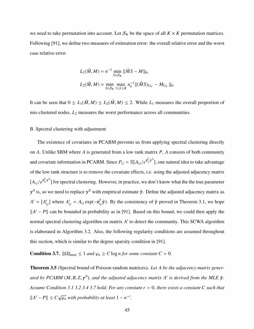
we need to take permutation into account. Let SK be the space of all K × K permutation matrices.
Following [91], we define two measures of estimation error: the overall relative error and the worst
case relative error:
L1(M,M) = n−1 minS∈SK‖MS − M ‖0,
L2(M,M) = minS∈SK
max1≤k≤K
n−1k ‖(MS)Gk · − MGk ·‖0.
It can be seen that 0 ≤ L1(M,M) ≤ L2(M,M) ≤ 2. While L1 measures the overall proportion of
mis-clustered nodes, L2 measures the worst performance across all communities.
B. Spectral clustering with adjustment
The existence of covariates in PCABM prevents us from applying spectral clustering directly
on A. Unlike SBM where A is generated from a low rank matrix P, A consists of both community
and covariate information in PCABM. Since Pi j = E[Ai j/ezTijγ
0], one natural idea to take advantage
of the low rank structure is to remove the covariate effects, i.e. using the adjusted adjacency matrix
[Ai j/ezTijγ
0] for spectral clustering. However, in practice, we don’t know what the the true parameter
γ0 is, so we need to replace γ0 with empirical estimate γ. Define the adjusted adjacency matrix as
A′ = [A′i j] where A′i j = Ai j exp(−zTi j γ). By the consistency of γ proved in Theorem 3.1, we hope
‖A′ − P‖ can be bounded in probability as in [91]. Based on this bound, we could then apply the
normal spectral clustering algorithm on matrix A′ to detect the community. This SCWA algorithm
is elaborated in Algorithm 3.2. Also, the following regularity conditions are assumed throughout
this section, which is similar to the degree sparsity condition in [91].
Condition 3.7. ‖Ω‖max ≤ 1 and ϕn ≥ C log n for some constant C > 0.
Theorem 3.5 (Spectral bound of Poisson random matrices). Let A be the adjacency matrix gener-
ated by PCABM (M,B, Z,γ0), and the adjusted adjacency matrix A′ is derived from the MLE γ.
Assume Condition 3.1 3.2 3.4 3.7 hold. For any constant r > 0, there exists a constant C such that
‖A′ − P‖ ≤ C√ϕn with probability at least 1 − n−r .
45

Algorithm 3.2 PCABM.SCWAInput: adjacency matrix A, pairwise covariates Z , initial assignment e, likelihood functionL(e,γ, B, π), number of communities K and approximation parameter ε
Output: coefficient estimate γ and community estimate c1: Optimize `e(γ) by some optimization algorithm (e.g., BFGS) to derive γ.2: Divide Ai j by exp(zT
i j γ) to get A′i j .3: Calculate UA′ ∈ R
n×K consisting of the leading K eigenvectors (ordered in absolute eigen-value) of A′.
4: Calculate the (1+ε)-approximate solution (M, X) to the k-means problem (3.4) with K clustersand input matrix UA′.
5: Output c according to M .
With similar proof of Theorem 3.1 in [91], we can prove the following Theorem 3.6 by com-
bining Lemmas 5.1 and 5.3 in [91], and Theorem 3.5.
Theorem 3.6. Based on the conditions of Theorem 3.5, assume that P = MBMT is of rank K with
the smallest absolute non-zero eigenvalue at least ξn. Let M be the output of spectral clustering
using (1+ε) approximate k-means on A′. For any constant r > 0, there exists an absolute constant
C > 0, such that, if
(2 + ε)Knρn
ξ2n
< C,
then, with probability at least 1 − n−r , there exist subsets Hk ⊂ Gk for k = 1, · · · ,K , and a K × K
permutation matrix J such that MG·J = MG·, where G = ∪Kk=1(Gk \ Hk), and
K∑k=1
|Hk |
nk≤ C−1(2 + ε)
Knρn
ξ2n
. (3.5)
Inequality (3.5) provides an error bound for L2(M,M). In set Hk , the clustering accuracy of
nodes can not be guaranteed. Theorem 3.6 doesn’t provide us with an error bound in a straightfor-
ward form since ξn contains ρn. The following corollary gives us a clearer view of the error bound
in terms of model parameters.
Corollary 3.7. Based on the conditions of Theorem 3.5, assume Ω′s minimum absolute eigenvalue
bounded below by τ > 0 and ‖Ω‖max = 1. Let M be the output of spectral clustering using (1 + ε)
46

approximate k-means. For any constant r > 0, there exists an absolute constant C such that if
(2 + ε)Kn
n2minτ
2ρn< C,
then with probability at least 1 − n−r ,
L2(M,M) ≤ C−1(2 + ε)Kn
n2minτ
2ρnand L1(M,M) ≤ C−1(2 + ε)
Kn′max
n2minτ
2ρn.
The result provides us with the same convergence rate as in [91]. The intuition is that if we see
the covariate from an expectation view, then it’s just a constant multiplied to the original probabil-
ity, the rate of convergence shouldn’t be affected.
Algorithm 3.3 PCABM.MLEInput: adjacency matrix A, pairwise covariates Z , initial classes e, likelihood function
L(e,γ, B, π), number of communities K and approximation parameter ε
Output: coefficient estimate γ and community estimate c
1: Use Algorithm 3.2 to get an initial community estimate c.
2: Use c as the initial value in `γ(c) for tabu search to derive c.
Compared with SCWA, the likelihood tabu search usually leads to more precise results but
takes longer time. Also, the results of the likelihood tabu search are sensitive to the initial labels e
in some settings. To combine the advantages of those two methods, we propose to use the results
of SCWA as the initial solution for tabu search (PCABM.MLE as described in Algorithm 3.3),
which shows better empirical performance than each method alone. We will conduct extensive
simulation studies in Section 3.4.
3.4 Simulations
For all simulations, we consider K = 2 communities with prior probability π1 = π2 = 0.5. In
addition, we fix Ω =( 2 1
1 2)
and generate data by applying the following procedure:
47
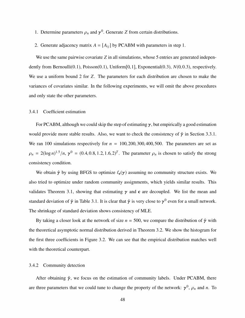
1. Determine parameters ρn and γ0. Generate Z from certain distributions.
2. Generate adjacency matrix A = [Ai j] by PCABM with parameters in step 1.
We use the same pairwise covariate Z in all simulations, whose 5 entries are generated indepen-
dently from Bernoulli(0.1), Poisson(0.1), Uniform[0,1], Exponential(0.3), N(0,0.3), respectively.
We use a uniform bound 2 for Z . The parameters for each distribution are chosen to make the
variances of covariates similar. In the following experiments, we will omit the above procedures
and only state the other parameters.
3.4.1 Coefficient estimation
For PCABM, although we could skip the step of estimating γ, but empirically a good estimation
would provide more stable results. Also, we want to check the consistency of γ in Section 3.3.1.
We ran 100 simulations respectively for n = 100,200,300,400,500. The parameters are set as
ρn = 2(log n)1.5/n, γ0 = (0.4,0.8,1.2,1.6,2)T . The parameter ρn is chosen to satisfy the strong
consistency condition.
We obtain γ by using BFGS to optimize `e(γ) assuming no community structure exists. We
also tried to optimize under random community assignments, which yields similar results. This
validates Theorem 3.1, showing that estimating γ and c are decoupled. We list the mean and
standard deviation of γ in Table 3.1. It is clear that γ is very close to γ0 even for a small network.
The shrinkage of standard deviation shows consistency of MLE.
By taking a closer look at the network of size n = 500, we compare the distribution of γ with
the theoretical asymptotic normal distribution derived in Theorem 3.2. We show the histogram for
the first three coefficients in Figure 3.2. We can see that the empirical distribution matches well
with the theoretical counterpart.
3.4.2 Community detection
After obtaining γ, we focus on the estimation of community labels. Under PCABM, there
are three parameters that we could tune to change the property of the network: γ0, ρn and n. To
48

Table 3.1: Simulated results for distribution of γ, displayed as mean (standard deviation)
n γ01 = 0.4 γ0
2 = 0.8 γ03 = 1.2 γ0
4 = 1.6 γ05 = 2
1000.4018 0.8003 1.1944 1.6153 2.0214
(0.0269) (0.0184) (0.0369) (0.0309) (0.0302)
2000.3929 0.7956 1.1648 1.5901 2.0057
(0.0139) (0.0117) (0.0228) (0.0151) (0.0205)
3000.4162 0.7953 1.1607 1.5962 1.9912
(0.0114) (0.0073) (0.0186) (0.0086) (0.0120)
4000.3931 0.8049 1.1960 1.6075 2.0122
(0.0091) (0.0057) (0.0144) (0.0081) (0.0097)
5000.3944 0.7998 1.2017 1.5970 2.0038
(0.0081) (0.0051) (0.0124) (0.0086) (0.0099)
Figure 3.2: Simulation results for γ compared with theoretical values
illustrate the impact of these parameters on the performance of community detection, we vary one
parameter while fixing the remaining two in each experiment. More specifically, we consider the
form ρn = cρ(log n)1.5/n and γ0 = cγ(0.4,0.8,1.2,1.6,2)T in which we will vary the multipliers cρ
and cγ. We also did one more experiment by plugging different γ into `γ(e) and estimate c. Here
we use one dimensional covariate following Poisson(0.1). The detailed parameter settings for the
four experiments are as follows.
1. n ∈ 100,200,300,400,500, with cρ = 0.5 and cγ = 1.4.
2. cρ ∈ 0.3,0.4,0.5,0.6,0.7, with n = 200 and cγ = 1.4.
3. cγ ∈ 0.2,0.4,0.6,0.8,1.0,1.2,1.4,1.6, with n = 200 and cρ = 1.
4. γ ∈ 0,0.5,1,1.5,2,2.5,3,3.5, with γ0 = 2, n = 500 and cρ = 1.
The results for the three experiments are presented in Figure 3.3. Each experiment is carried
out for 100 times. The error rate is reported in terms of average ARI. SBM.MLE and SBM.SC
49
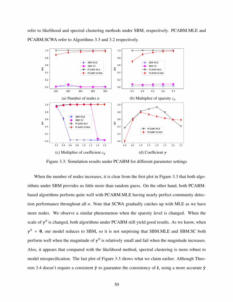
refer to likelihood and spectral clustering methods under SBM, respectively. PCABM.MLE and
PCABM.SCWA refer to Algorithms 3.3 and 3.2 respectively.
(a) Number of nodes n (b) Multiplier of sparsity cρ
(c) Multiplier of coefficient cγ (d) Coefficient γ
Figure 3.3: Simulation results under PCABM for different parameter settings
When the number of nodes increases, it is clear from the first plot in Figure 3.3 that both algo-
rithms under SBM provides us little more than random guess. On the other hand, both PCABM-
based algorithms perform quite well with PCABM.MLE having nearly perfect community detec-
tion performance throughout all n. Note that SCWA gradually catches up with MLE as we have
more nodes. We observe a similar phenomenon when the sparsity level is changed. When the
scale of γ0 is changed, both algorithms under PCABM still yield good results. As we know, when
γ0 = 0, our model reduces to SBM, so it is not surprising that SBM.MLE and SBM.SC both
perform well when the magnitude of γ0 is relatively small and fail when the magnitude increases.
Also, it appears that compared with the likelihood method, spectral clustering is more robust to
model misspecification. The last plot of Figure 3.3 shows what we claim earlier. Although Theo-
rem 3.4 doesn’t require a consistent γ to guarantee the consistency of c, using a more accurate γ
50
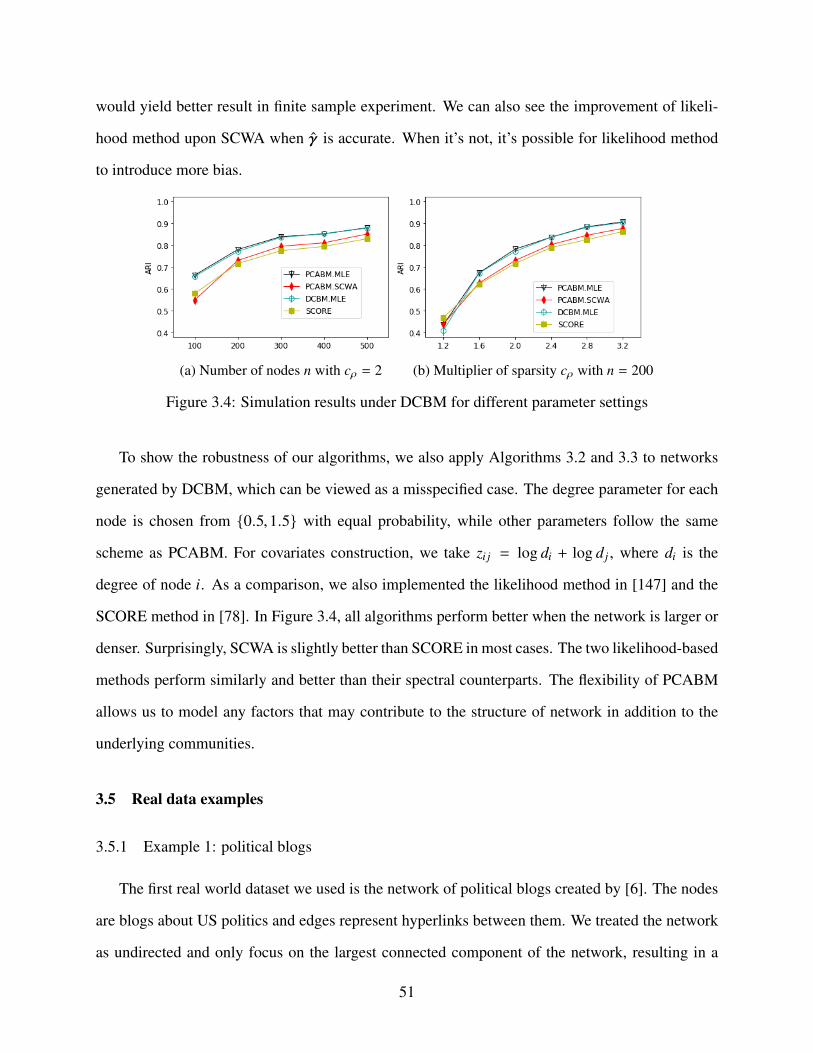
would yield better result in finite sample experiment. We can also see the improvement of likeli-
hood method upon SCWA when γ is accurate. When it’s not, it’s possible for likelihood method
to introduce more bias.
(a) Number of nodes n with cρ = 2 (b) Multiplier of sparsity cρ with n = 200
Figure 3.4: Simulation results under DCBM for different parameter settings
To show the robustness of our algorithms, we also apply Algorithms 3.2 and 3.3 to networks
generated by DCBM, which can be viewed as a misspecified case. The degree parameter for each
node is chosen from 0.5,1.5 with equal probability, while other parameters follow the same
scheme as PCABM. For covariates construction, we take zi j = log di + log d j , where di is the
degree of node i. As a comparison, we also implemented the likelihood method in [147] and the
SCORE method in [78]. In Figure 3.4, all algorithms perform better when the network is larger or
denser. Surprisingly, SCWA is slightly better than SCORE in most cases. The two likelihood-based
methods perform similarly and better than their spectral counterparts. The flexibility of PCABM
allows us to model any factors that may contribute to the structure of network in addition to the
underlying communities.
3.5 Real data examples
3.5.1 Example 1: political blogs
The first real world dataset we used is the network of political blogs created by [6]. The nodes
are blogs about US politics and edges represent hyperlinks between them. We treated the network
as undirected and only focus on the largest connected component of the network, resulting in a
51

network with 1,222 nodes and 16,714 edges.
Because there are no other covariates available in this dataset, we created the pairwise covari-
ates by aggregating the degree information. We let zi j = log(di × d j), where di is the degree for the
i-th node. The corresponding γ is 1.001, which essentially reduces PCABM to DCBM. Table 3.2
summarizes the performance comparison of PCABM with some existing results on this dataset.
Besides ARI, we also evaluated normalized mutual information (NMI) [47], which is a measure
of the mutual dependence between the two variables. It is observed that our model slightly out-
performs all previous results and the error rate is very close to the ideal results mentioned in [78],
which is 55/1222. This shows that PCABM can effectively incorporate the degree information into
a specific pairwise covariate and provide significant improvement over the vanilla SBM, whose
NMI is only 0.0001 as reported in [80].
Table 3.2: Performance comparison on political blogs data
ARI NMI ErrorsKarrer and Newman (2011) [80] - 0.72 -
Zhao et al. (2012) [147] 0.819 - -Jin (2015) [78] 0.819 0.725 58PCABM.MLE 0.825 0.737 56
3.5.2 Example 2: school friendship
For real networks, people often use certain nodal labels as the ground ‘truth’ for community
labels to evaluate the performance of various community detection methods. However, there could
be different ‘true’ community assignments based on different nodal labels (e.g., gender, job, and
age). [115] mentioned that communities and the covariates may capture different aspects of the
network, which is inline with the idea presented here. To examine whether PCABM can discover
different community structures, in our second example, we treat one covariate as the indicator for
the unknown ‘true’ community assignments while using the remaining covariates as the known
covariates in our PCABM model.
The dataset is a friendship network of school students, which is from the National Longitudinal
52

Study of Adolescent to Adult Health (Add Health). It contains 795 students from a high school
(Grades 9-12) and its feeder middle school (Grade 7-8). The pairwise covariates include grade,
gender, ethnicity and number of friends nominated (up to 10). We focused on the largest connected
component with at least one covariate non-missing and treat the network as undirected, resulting in
a network with 777 nodes and 4124 edges. For the nodes without gender, we let them to be female,
which is the smaller group. For those without grade, we generated a random grade according to
their schools.
Different from traditional community detection algorithms which can only detect one underly-
ing community structure, PCABM provides us with more flexibility to uncover different commu-
nity structures by controlling different covariates. Our intuition is that social network is usually
determined by multiple underlying structures, so it cannot be simply explained by one covariate.
Sometimes one community structure seems to dominate the network, but if we control the covariate
associated with this structure, we may discover other interesting community structures.
In this example, we conducted three community detection experiments. In each experiment,
out of the three nodal labels (school, ethnicity and gender), one was viewed as the indicator for the
underlying community, and community detection was carried out by using the pairwise covariates
constructed using the other two covariates. For gender, school and ethnicity, we created indicator
variables to represent whether the corresponding covariate values were the same for the pair of
nodes. Besides, we considered the number of nominated friends in all experiments and grade for
predicting ethnicity and gender. For number of nominated friends, we used log(ni +1)+ log(n j +1)
as one pairwise covariate, where ni is the number of nominated friends for the i-th student. ‘+1’
was used here because some students didn’t nominate anyone. For grades, we used the absolute
difference to form a pairwise covariate. Using random initial community labels, we derived the
estimates γ in each experiment. In Tables 3.3 and 3.4, we show respectively the estimates when
school and ethnicity are taken as the targeted community.
In both tables, the standard error is calculated by Theorem 3.2, with the theoretical values
replaced by the estimated counterparts. Thus, we can calculate the t value for each coefficient
53

Table 3.3: Inference results when school is targeted community
Covariate Estimate Std. Error t value Pr(> |t|)White 1.251 0.043 29.002 < 0.001***Black 1.999 0.051 38.886 < 0.001***
Hispanic 0.048 0.523 0.091 0.927Others 0.019 0.543 0.035 0.972Gender 0.192 0.034 -5.620 < 0.001***
Nomination 0.438 0.024 18.584 < 0.001***
Table 3.4: Inference results when ethnicity is targeted community
Covariate Estimate Std. Error t value Pr(> |t|)School 1.005 0.076 -13.168 < 0.001***Grade -1.100 0.028 -39.182 < 0.001***Gender 0.198 0.034 -5.813 < 0.001***
Nomination 0.498 0.023 21.679 < 0.001***
and perform statistical tests. We can see that in both experiments, the coefficients for gender and
the number of nominations are similar. They both appear to be significant in the creation of the
friendship network. The significant positive coefficient of nominations shows that students with a
large number of nominations tend to be friends with each other, which is intuitive. The positive
coefficients of gender and school shows students of the same gender and school are more likely
to be friends with each other, which is in line with our expectations. The negative coefficient of
grade means that students with closer grades are more likely to be friends with each other. If we
take a closer look at the coefficients of different ethnic groups in Table 3.3, we find that only those
corresponding to white and black are significant. This is understandable if we observe that among
777 students, 476 are white and 221 are black. As for school and grade, students in the same school
or grade are more likely to be friends with each other, which is as we expected.
The network is divided into two communities each time (we only look at white and black stu-
dents in the second experiment because the sizes for other ethnicities are very small). In Figure 3.5,
school, ethnicity and gender are targeted communities respectively. We use different shades to dis-
tinguish true communities. Predicted communities are separated by the middle dash line, so the
ideal split would be shades vs. tints on two sides. By this criteria, our model performs pretty
54

well for the first two cases, but fails to distinguish different genders. Also, more edges between
two communities in the third plot indicates bad performance. It can either be the existence of an-
other unknown variables or gender’s contribution to the network structure is insignificant given the
covariates considered.
The results in terms of ARI are shown in Table 3.5. Note that, for all other methods, we would
get only one community structure, whose performance is doomed to be bad for capturing different
community structures. Also, to test the robustness of our method, in the experiment of detecting
the ethnicity community, we tried to use the square of the grade difference which led to almost the
same ARI.
Table 3.5: ARI comparison on school friendship data
School Race GenderPCABM.MLE 0.909 0.914 0.030
SBM.MLE 0.048 0.138 -0.001SBM.SC 0.043 -0.024 0.000
DCBM.MLE 0.909 0.001 0.002SCORE 0.799 0.012 0.011
3.6 Discussion
In this chapter, we extended the classical stochastic block model to let the connection probabil-
ity between nodes not only depend on communities but also on the pairwise covariates. We proved
consistency in terms of both coefficient estimates and community label assignments for MLE under
PCABM. Also, we introduced a fast spectral method SCWA with theoretical justification, which
may serve as a good initial solution for the likelihood method.
Though we assumed Ai j’s are non-negative integers, it can be relaxed to be any non-negative
number, and the proof still holds. Also, we would like to consider unbalanced community sizes
nmin/nmax = o(1) or when the number of communities Kn diverges.
One possible future work is to extend PCABM to directed network. Besides, for the bounded
degree case where ϕn = O(1), it is of great interest to discuss the properties of estimators under
55
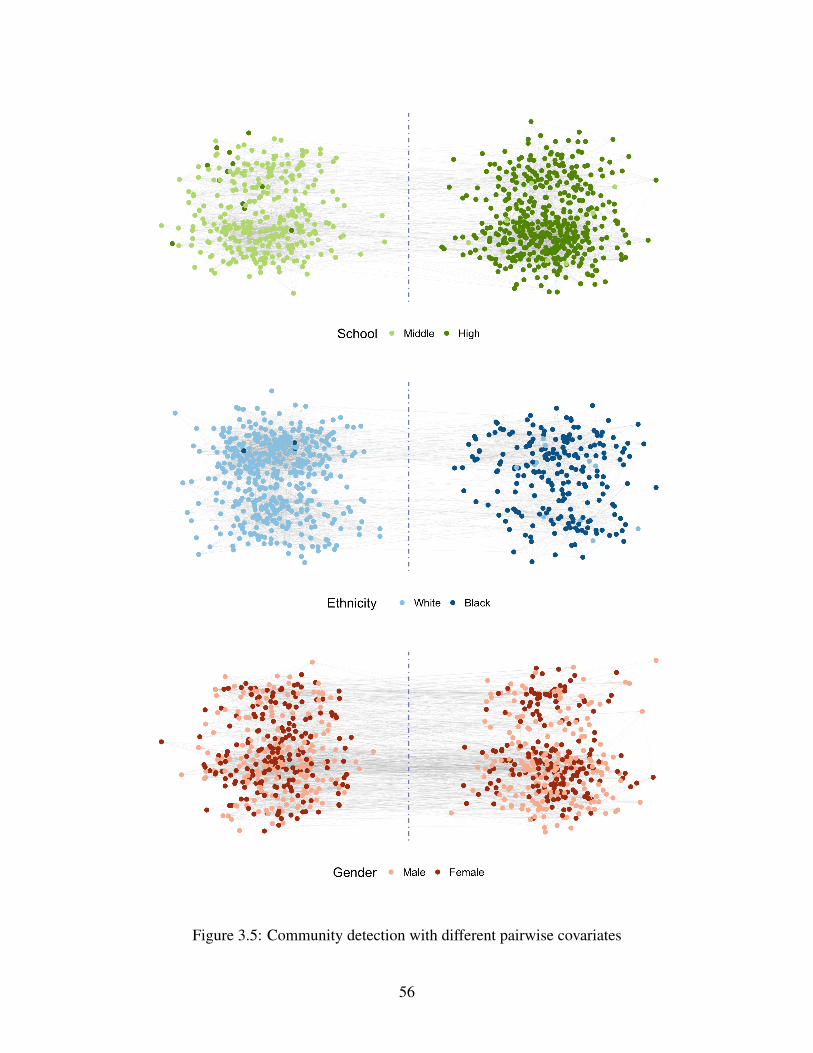
Figure 3.5: Community detection with different pairwise covariates
56

our framework. When we have high-dimensional pairwise covariates, adding a penalty term to
perform variable selection is also worth investigating.
Another interesting issue is the choice of the number of communities K which is assumed to
be known in this thesis. However, in practice, it would be desirable to have an automatic selection
procedure for choosing K . Some recent efforts toward this direction include [121, 87, 134, 90, 39,
92, 143]. It would be interesting to study some of the methods under PCABM.
3.7 Proofs
This section contains proofs of Theorems 3.1, 3.2, 3.3, 3.4 and 3.5.
3.7.1 Proof of Theorem 3.1 and Theorem 3.2
Proof. In the following proof, we will use γ instead of γ(e) for simplicity. Define the empirical
version of θ(γ), µ(γ) and Σ(γ) as
θkl(γ) =∑
(u,v)∈se(k,l)
ezTuvγ/|se(k, l)|,
µkl(γ) =∑
(u,v)∈se(k,l)
zuvezTuvγ/|se(k, l)|,
Σkl(γ) =
∑(u,v)∈se(k,l)
zuvzTuvezTuvγ/|se(k, l)|.
For fixed γ, under Condition 3.1 and 3.4, for ∀k, l ∈ [K], we know the weak law of large numbers
holds, i.e., θkl(γ)p−→ θ(γ), µkl(γ)
p−→ µ(γ) and Σkl(γ)
p−→ Σ(γ).
First, we calculate the first and second order derivative of `e w.r.t. γ as
`′e(γ) =∂`e∂γ=
∑i< j
Ai jzi j −∑i< j
Ai j µeiej (γ)/θeiej (γ),
`′′e (γ) =∂2`e
∂γ∂γT =∑kl
Okl(e)2θkl(γ)2
[µkl(γ)⊗2 − θkl(γ)Σkl(γ)
].
Then conditioned on Z , we define the expectation and variance of `′e(γ) as µ`(e,γ) = E[`′e(γ)|Z]
57
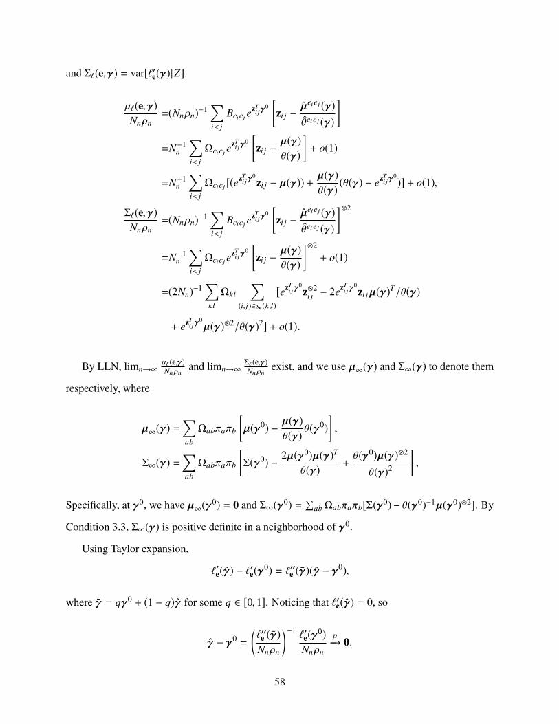
and Σ`(e,γ) = var[`′e(γ)|Z].
µ`(e,γ)Nnρn
=(Nnρn)−1
∑i< j
Bcicj ezTijγ
0[zi j −
µeiej (γ)
θeiej (γ)
]=N−1
n
∑i< j
Ωcicj ezTijγ
0[zi j −
µ(γ)
θ(γ)
]+ o(1)
=N−1n
∑i< j
Ωcicj [(ezTijγ
0zi j − µ(γ)) +
µ(γ)
θ(γ)(θ(γ) − ezTijγ
0)] + o(1),
Σ`(e,γ)Nnρn
=(Nnρn)−1
∑i< j
Bcicj ezTijγ
0[zi j −
µeiej (γ)
θeiej (γ)
]⊗2
=N−1n
∑i< j
Ωcicj ezTijγ
0[zi j −
µ(γ)
θ(γ)
]⊗2+ o(1)
=(2Nn)−1
∑kl
Ωkl
∑(i,j)∈sc(k,l)
[ezTijγ0z⊗2
i j − 2ezTijγ0zi jµ(γ)
T/θ(γ)
+ ezTijγ0µ(γ)⊗2/θ(γ)2] + o(1).
By LLN, limn→∞µ`(e,γ)Nnρn
and limn→∞Σ`(e,γ)Nnρn
exist, and we use µ∞(γ) and Σ∞(γ) to denote them
respectively, where
µ∞(γ) =∑ab
Ωabπaπb
[µ(γ0) −
µ(γ)
θ(γ)θ(γ0)
],
Σ∞(γ) =∑ab
Ωabπaπb
[Σ(γ0) −
2µ(γ0)µ(γ)T
θ(γ)+θ(γ0)µ(γ)⊗2
θ(γ)2
],
Specifically, at γ0, we have µ∞(γ0) = 0 and Σ∞(γ0) =
∑abΩabπaπb[Σ(γ
0) − θ(γ0)−1µ(γ0)⊗2]. By
Condition 3.3, Σ∞(γ) is positive definite in a neighborhood of γ0.
Using Taylor expansion,
`′e(γ) − `′e(γ
0) = `′′e (γ)(γ − γ0),
where γ = qγ0 + (1 − q)γ for some q ∈ [0,1]. Noticing that `′e(γ) = 0, so
γ − γ0 =
(`′′e (γ)
Nnρn
)−1 `′e(γ0)
Nnρn
p−→ 0.
58

To prove asymptotic normality, we rewrite above formula as
√Nnρn(γ − γ
0) = −
[1
Nnρn`′′e (γ)
]−1×
[1
√Nnρn
`′e(γ0)
].
Since γp−→ γ0, we have Nnρn`
′′−1e (γ)
p−→ Σ2(γ
0). Also, conditioned on Z , by C.L.T.,
1√
Nnρn`′e(γ
0) =√
Nnρn
[1
Nnρn`′e(γ
0)
]d−→ N(0,Σ2(γ
0)).
Thus, √Nnρn(γ − γ
0)d−→ N(0,Σ−1
∞ (γ0)).
3.7.2 Some concentration inequalities and notations
For the purpose of later proofs, we introduce some concentration inequalities and necessary
notations first.
One inequality that we will apply repeatedly is extended version of Bernstein inequality for
unbounded random variables introduced in [138].
Lemma 3.8 (Bernstein inequality). Suppose X1, · · · ,Xn are independent random variables with
EXi = 0 and E|Xi |k ≤ 1
2EX2i Lk−2k! for k ≥ 2. For M ≥
∑i≤n EX2
i and x ≥ 0,
Pr
(∑i≤n
Xi ≥ x
)≤ exp
(−
x2
2(M + xL)
).
To show that all Poisson distributions satisfy the above Bernstein condition uniformly under
some constant L, we give the following lemma.
Lemma 3.9 (Bernstein condition). Assume A ∼ Pois(λ), let X = A− λ, then for any 0 < λ < 1/2,
there exists a constant L > 0 s.t. for any integer k > 2, E[|X k |] ≤ E[X2]Lk−2k!/2.
59

Proof.
2E[|A − λ |k]λk!
=2λk!E[(A − λ)k |A ≥ 1]Pr(A ≥ 1) +
2λk−1e−λ
k!
≤2λk!E[Ak |A ≥ 1]Pr(A ≥ 1) + e−λ =
2λk!E[Ak] + e−λ
2k!
k∑i=1
k
i
λi−1 + e−λ
≤1k!
k∑i=1
(ki
)ik−iλi−1 + e−λ ≤
ek−1
k k
k∑i=1
(eki
) i
ik−iλi−1 + e−λ
=
k∑i=1
ei+k−1ik−2i ki−kλi−1 + e−λ <k∑
i=1ei+k−1e−iλi−1 + e−λ = ek−1 1 − λk
1 − λ+ e−λ
≤ek−1
1 − λ+ 1 ≤
(e2 + 11 − λ
) k−2
.
Notice that when λ is bounded away from 1, say λ < 1/2, we can simply set L = 2(e2 + 1), then
Bernstein condition is satisfied uniformly for all λ.
We introduce some notations. Let |e − c| =∑n
i=1 1ei,ci . Given a community assignment
e ∈ [K]n, we define V(e) ∈ RK×K with its elements being
Vka(e) ≡∑n
i=1 1ei=k,ci=a∑ni=1 1ci=a
=Rka(e)πa(c)
.
One can view V as the empirical conditional distribution of e given c. We can see that V(e) =
R(e)D(c)−1. Also, note that V(e)T1 = 1, V(e)π(c) = π(e) and V(c) = IK . For the convenience of
later proof, we also define W(c) = D(c)ΩD(c) and
T(e) ≡R(e)ΩR(e)T = V(e)W(c)V(e)T,
S(e) ≡V(e)π(c)π(c)TV(e)T .
Replacing the empirical distribution π(c) by the true distribution π, we define W0 = D(π)ΩD(π),
60

and T(e),S(e) ∈ RK×K as
T(e) ≡V(e)W0V(e)T,
S(e) ≡V(e)ππTV(e)T .
The population version of F(
O2Nnρn
, E2Nn
)is F(θ(γ0)T(e), θ(γ)S(e)). To measure the discrep-
ancy between empirical and population version of F, we define X(e),Y (e, γ) ∈ RK×K to be the
rescaled difference between O,E and their expectations
X(e) ≡O(e)
2Nnρn− θ(γ0)T(e),
Y (e, γ) ≡E(e, γ)
2Nn− θ(γ)S(e).
Before we establish bound for Y (e, γ), we need to consider the bound for γ. The following is
a direct corollary of Theorem 3.2. Conditioned on ‖γ − γ0‖∞ ≤ φ, we have |ezi j γ − Eezi j γ | ≤
exppα(φ + ‖γ0‖∞) ≡ χ uniformly for any i, j ∈ [n] and γ. Under this condition, we establish
Lemma 3.11 using Bernstein inequality.
Lemma 3.10. For any constant φ > 0, ∃ positive constants Cφ and vφ s.t., Pr(‖γ − γ0‖∞ > φ) <
Cφ exp(−vφNnρn).
Lemma 3.11.
Pr(maxe‖X(e)‖∞ ≥ ε) ≤ 2Kn+2 exp(−C1ε
2Nnρn) (3.6)
for ε < βu‖Ω‖max/L.
Pr( max|e−c|≤m
‖X(e) − X(c)‖∞ ≥ ε) ≤ 2(
nm
)Km+2 exp
(−
C3nm
ε2Nnρn
)(3.7)
61
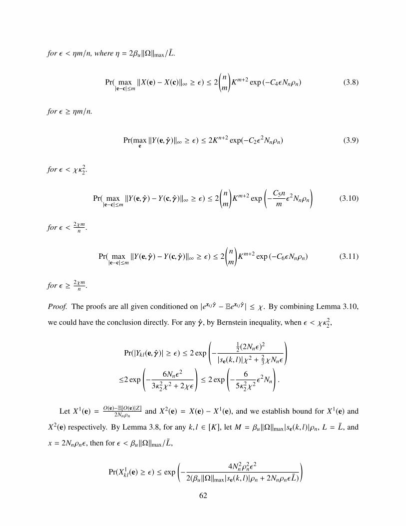
for ε < ηm/n, where η = 2βu‖Ω‖max/L.
Pr( max|e−c|≤m
‖X(e) − X(c)‖∞ ≥ ε) ≤ 2(
nm
)Km+2 exp (−C4εNnρn) (3.8)
for ε ≥ ηm/n.
Pr(maxe‖Y (e, γ)‖∞ ≥ ε) ≤ 2Kn+2 exp(−C2ε
2Nnρn) (3.9)
for ε < χκ22 .
Pr( max|e−c|≤m
‖Y (e, γ) − Y (c, γ)‖∞ ≥ ε) ≤ 2(
nm
)Km+2 exp
(−
C5nm
ε2Nnρn
)(3.10)
for ε < 2χmn .
Pr( max|e−c|≤m
‖Y (e, γ) − Y (c, γ)‖∞ ≥ ε) ≤ 2(
nm
)Km+2 exp (−C6εNnρn) (3.11)
for ε ≥ 2χmn .
Proof. The proofs are all given conditioned on |ezi j γ − Eezi j γ | ≤ χ. By combining Lemma 3.10,
we could have the conclusion directly. For any γ, by Bernstein inequality, when ε < χκ22 ,
Pr(|Ykl(e, γ)| ≥ ε) ≤ 2 exp
(−
12 (2Nnε)
2
|se(k, l)|χ2 + 23 χNnε
)≤2 exp
(−
6Nnε2
3κ22 χ
2 + 2χε
)≤ 2 exp
(−
65κ2
2 χ2ε2Nn
).
Let X1(e) = O(e)−E[O(e)|Z]2Nnρn
and X2(e) = X(e) − X1(e), and we establish bound for X1(e) and
X2(e) respectively. By Lemma 3.8, for any k, l ∈ [K], let M = βu‖Ω‖max |se(k, l)|ρn, L = L, and
x = 2Nnρnε , then for ε < βu‖Ω‖max/L,
Pr(X1kl(e) ≥ ε) ≤ exp
(−
4N2n ρ
2nε
2
2(βu‖Ω‖max |se(k, l)|ρn + 2Nnρnε L)
)62

≤ exp(−
Nnρnε2
βu‖Ω‖max + ε L
)≤ exp
(−
ε2Nnρn
2βu‖Ω‖max
).
Notice that |X2kl(e)|/‖Ω‖max ≤ |Ykl(e,γ0)|. Thus, for ε < χκ2
2 ‖Ω‖max,
Pr(|X2kl(e)| ≥ ε) ≤Pr
(|Ykl(e,γ0)| ≥
ε
‖Ω‖max
)≤ 2 exp
(−
65κ2
2 χ2‖Ω‖max
ε2Nn
).
Thus, the bound of X(e) will be dominated by X1(e), and we will ignore the second term in the
bound because it is just a small order and can be absorbed into the first one.
Similar to the arguments in [147], for |e − c| ≤ m, ε < 2χmn ,
Pr(|Ykl(e, γ) − Ykl(c, γ)| ≥ ε) ≤ 2 exp(−
6Nnε2
6χ2mn/Nn + 2χε
)≤2 exp
(−
3(n − 1)8χ2m
ε2Nn
)≤ 2 exp
(−
n4χ2m
ε2Nn
).
For ε ≥ 2χmn ,
Pr(|Ykl(e, γ) − Ykl(c, γ)| ≥ ε) ≤ 2 exp(−
6Nnε2
6χ2mn/Nn + 2χε
)≤ 2 exp
(−
34χ
εNn
).
Also, for ε < 2βu ‖Ω‖maxmnL ,
Pr(|X1kl(e) − X1
kl(c)| ≥ ε) ≤ exp(−
Nnρnε2
βu‖Ω‖maxmn/Nn + ε L
)≤ exp
(−
n − 12βu‖Ω‖maxm
ε2Nnρn
)≤ exp
(−
n4βu‖Ω‖maxm
ε2Nnρn
).
For ε ≥ 2βu ‖Ω‖maxmnL ,
Pr(|X1kl(e) − X1
kl(c)| ≥ ε) ≤ exp(−
Nnρnε2
βu‖Ω‖maxmn/Nn + ε L
)≤ exp
(−
13L
εNnρn
).
We will omit the bound for |X2kl(e) − X2
kl(c)| since it’s a smaller order.
63
3.7.3 Proof of Theorem 3.3
Proof. We divide the proof into three steps.
Step 1 : sample and population version comparison. We prove ∃ εn → 0, such that
P(max
e
F (O(e)
2Nnρn,
E(e, γ)2Nn
)− F(θ(γ0)T(e), θ(γ0)S(e))
≤ εn
)→ 1, (3.12)
if ϕn →∞ and γp−→ γ0.
Since F (O(e)
2Nnρn,
E(e, γ)2Nn
)− θ(γ0)F(T(e),S(e))
≤
F (O(e)
2Nnρn,
E(e, γ)2Nn
)− F(θ(γ0)T(e), θ(γ)S(e))
+
F(θ(γ0)T(e), θ(γ)S(e)) − θ(γ0)F(T(e), S(e))
+ θ(γ0)F(T(e), S(e)) − F(T(e),S(e))
,it is sufficient to bound these three terms uniformly. By Lipschitz continuity,F (
O(e)2Nnρn
,E(e, γ)
2Nn
)− θ(γ0)F
(T(e), S(e)
) ≤ M1‖X(e)‖∞ + M2‖Y (e, γ)‖∞, (3.13)F(θ(γ0)T(e), θ(γ)S(e)) − θ(γ0)F(T(e), S(e)) ≤ M2 |θ(γ) − θ(γ
0)|‖S(e)‖∞. (3.14)
By (3.6) and (3.9), (3.13) converges to 0 uniformly if ϕn → ∞. Since ‖S(e)‖∞ is uniformly
bounded by 1, (3.14) also converges to 0 uniformly.
F (T(e), S(e)
)− F (T(e),S(e))
≤ M1‖T(e) − T(e)‖∞ + M2‖S(e) − S(e)‖∞. (3.15)
Since π(c)p−→ π, (3.15) converges to 0 uniformly. So we prove (3.12).
64
Step 2 : proof of weak consistency. We prove that there exists δn → 0, such that
Pr(
maxe:‖V(e)−IK ‖1≥δn
F(
O(e)2Nnρn
,E(e, γ)
2Nn
)< F
(O(c)
2Nnρn,
E(c, γ)2Nn
))→ 1. (3.16)
By continuity property of F and Condition 3.5, there exists δn → 0, such that
θ(γ0)F(T(c),S(c)) − θ(γ0)F(T(e),S(e)) > 2εn
if ‖V(e) − IK ‖1 ≥ δn, where IK = V(c). Thus, following (3.12),
Pr
(max
e:‖V(e)−IK ‖1≥δnF
(O(e)
2Nnρn,
E(e, γ)2Nn
)< F
(O(c)
2Nnρn,
E(c, γ)2Nn
) )≥Pr
( maxe:‖V(e)−IK ‖1≥δn
θ(γ0)F(T(e),S(e)) − maxe:‖V(e)−IK ‖1≥δn
F(
O(e)2Nnρn
,E(e, γ)
2Nn
) ≤ εn,θ(γ0)F(T(c),S(c)) − F(
O(c)2Nnρn
,E(c, γ)
2Nn
) ≤ εn
)→ 1.
(3.16) implies Pr(‖V(e) − IK ‖ < δn) → 1. Since
1n|e − c| =
1n
n∑i=1
1ci,ei =∑
k
πk(1 − Vkk(e)) ≤∑
k
(1 − Vkk(e)) = ‖V(e) − IK ‖1/2,
weak consistency follows.
Step 3 : proof of strong consistency.
To prove strong consistency, we need to show
Pr(
maxe:0<‖V(e)−IK ‖1<δn
F(
O(e)2Nnρn
,E(e, γ)
2Nn
)< F
(O(c)
2Nnρn,
E(c, γ)2Nn
))→ 1. (3.17)
Combining (3.16) and (3.17), we have
Pr(
maxe:e,c
F(
O(e)2Nnρn
,E(e, γ)
2Nn
)< F
(O(c)
2Nnρn,
E(c, γ)2Nn
))→ 1,
65
which implies strong consistency.
By Lipschitz continuity and the continuity of derivative of F w.r.t. V(e) in the neighborhood of
IK , we have
F(
O(e)2Nnρn
,E(e, γ)
2Nn
)− F
(O(c)
2Nnρn,
E(c, γ)2Nn
)=θ(γ0)F(T(e), S(e)) − θ(γ0)F(T(c), S(c)) + ∆(e,c),
(3.18)
where |∆(e,c)| ≤ M3(‖X(e) − X(c)‖∞) + M4‖Y (e, γ) − Y (c, γ)‖∞), and
F(T(e),S(e)) − F(T(c),S(c)) ≤ −C‖V(e) − I ‖1 + o(‖V(e) − IK ‖1).
Since the derivative of F is continuous w.r.t. V(e) in the neighborhood of IK , there exists a δ′
such that,
F(T(e), S(e)) − F(T(c), S(c)) ≤ −(C/2)‖V(e) − I ‖1 + o(‖V(e) − IK ‖1) (3.19)
holds when ‖π(c) − π‖∞ ≤ δ′. Since π(c) → π, (3.19) holds with probability approaching 1.
Combining (3.18) and (3.19), it is easy to see strong consistency follows if we can show
Pr(maxe,c|∆(e,c)| ≤ C‖V(e) − IK ‖1/4
)→ 1.
Note 1n |e − c| ≤ 1
2 ‖V(e) − IK ‖1. So for each m ≥ 1,
Pr(
max|e−c|=m
|∆(e,c)| > C‖V(e − IK)‖1/4)
≤Pr(
max|e−c|≤m
‖X(e) − X(c)‖∞ >Cm
4M3n
)(≡ I1)
+ Pr(
max|e−c|≤m
‖Y (e, γ) − Y (c, γ)‖∞ >Cm
4M4n
)(≡ I2).
(3.20)
66
Let ζ1 = C/4M3, if ζ1 < η, by (3.7),
I1 ≤2Km+2nm exp(−η2
1C3m
nNnρn
)= 2K2[K exp(log n − η2
1C3Nnρn/n)]m.
If ζ1 > η, by (3.8),
I1 ≤2Km+2nm exp(−η1
C4mn
Nnρn
)= 2K2[K exp(log n − η1C4Nnρn/n)]m.
Similar arguments hold for I2 by using (3.10) and (3.11). In all cases, since ϕn/log n→∞,
Pr(maxe,c|∆(e,c)| > C‖V(e) − IK ‖1/4
)=
∞∑m=1
Pr(
max|e−c|=m
|∆(e,c)| > C‖V(e) − IK ‖1/4)→ 0.
as n→∞. The proof is completed.
3.7.4 Proof of Theorem 3.4
By scaling `γ(e), we have
1Nn`γ(e) = ρnF
(O
2Nnρn,
E2Nn
)+ (ρn log ρn)
∑kl
Okl(e)2Nnρn
+O(n−1),
where F(X,Y ) =∑
kl Xkl log(
Xkl
Ykl
), X,Y ∈ RK×K . Note that F is closely related to the likelihood
criterion used in [147]. In our case,
F(θ(γ0)RΩRT, θ(γ0)ππT ) − F(θ(γ0)RΩRT, θ(γ)ππT )
=θ(γ0) logθ(γ0)
θ(γ)(1T RΩRT1),
which is basically the population degree up to a constant. This fact shows that the consistency
of γ is unnecessary to ensure the consistency of community detection. Thus, we can plug in any
67

random fixed γ, which is different from our general theorem. For simplicity, just assume we use
the true value γ0 here. Observe that
F(θ(γ0)RΩRT, θ(γ0)ππT ) = θ(γ0)F(RΩRT,ππT ),
then the form of F is exactly the same as F defined in [24], which automatically satisfies all
conditions for F.
3.7.5 Proof of Theorem 3.5
This proof is adapted from [91]. First, as a direct corollary of Theorem 3.2, we have the
following estimation error bound for γ.
Lemma 3.12. For any constant η > 0, ∃ positive constants Cη and vη s.t., Pr(√nρn‖γ0 − γ‖∞ >
η) < Cη exp(−vηn).
The following notations will be used in the proof.
• W = A′ − P and denote by wi j the (i, j)-th entry of W .
• For t > 0, let St = x ∈ Rn : ‖x‖2 ≤ t be the Euclidean ball of radius t and set S = S1.
The proof of Theorem 3.5 is adapted from [91], so we will skip the common part and only
clarify the modifications. The main idea is to bound
supx∈S|xT (A′ − P)x|. (3.21)
The original proof consists of three steps: discretization, bounding the light pairs and bounding
the heavy pairs. Discretization is to reduce 3.21 to the problem of bounding the supremum of
xT (A′− P)y for x,y in a finite set of grid points in S. Then we divide x,y into light and heavy pairs
and bound them respectively. We will focus on the last two steps since the first step is the same as
in [91].
68

A. Discretization
For fixed δn ∈ (0,1), define
T = x = (x1, · · · , xn) ∈ S :√
nxi/δn ∈ Z,∀i,
where Z stands for the set of integers. The following lemma is the same as Lemma B.1 in [91] and
we will skip the proof.
Lemma 3.13. S1−δn ⊂ convhull(T ). As a consequence, for all W ∈ Rn×n,
‖W ‖ ≤ (1 − δn)−2 sup
x,y∈T|xTWy|.
For any x,y ∈ T , we have
xT (A′ − P)y =∑
1≤i,j≤n
xiy j(A′i j − Pi j).
We only need bound the above quantity now. We divide (xi, y j) into light pairs L = (i, j) : |xiy j | ≤
√ϕn/n and heavy pairs H = (i, j) : |xiy j | >
√ϕn/n. We will show that the tail for light pairs
can be bounded exponentially while heavy pairs have a heavier tail. Thus, the rate of the latter one
dominates.
B. Bounding the light pairs
Lemma 3.14. Under estimation error condition, for c > 0, there exist constants Cc, vc > 0 s.t.
P ©« supx,y∈T
∑(i,j)∈L(x,y)
xiy jwi j
≥ c√ϕn
ª®¬ ≤ Cc exp[−
(vc − log
(7δ
))n].
Proof. Define w′i j = Ai je−zTijγ
0−Pi j and δi j = Ai je
−zTij γ− Ai je−zTijγ
0, then wi j = w′i j +δi j , and notice
69

that
Pr(∑
wi j > 2t) ≤ Pr(∑
w′i j > t) + Pr(∑
δi j > t),
so we could bound two parts respectively. Also, we need to keep in mind that
∑i< j
u2i j ≤
∑i< j
2(x2i y
2j + x2
j y2i ) ≤ 2
∑1≤i,j≤n
x2i y
2j = 2‖x‖22 ‖y‖
22 ≤ 2.
Step1 : Bound w′i j .
Since
∑i< j
E[(w′i jui j)2 |zi j] =
∑i< j
u2i jλi je
−2zTijγ0=
∑i< j
u2i j Pi je
−zTijγ0
≤ρnβ−1l ‖Ω‖max
∑i< j
u2i j ≤ 2β−1
l ‖Ω‖maxρn,
define M = 2β−1l ‖Ω‖maxρn, L = 2L
√ϕn(nβl)
−1 and x = c√ϕn, we could applying Lemma 3.8 to
ui jw′i j to get
Pr
(∑i< j
w′i jui j ≥ c√ϕn
)≤ exp
(−
c2ϕn
4cLϕn(nβl)−1 + 4ρnβ
−1l ‖Ω‖max
)= exp
(−
c2βln4cL + 4‖Ω‖max
)Step2 : Bound δi j .
We consider two cases ‖γ0−γ‖∞ > η/√
nρn and ‖γ0−γ‖∞ ≤ η/√
nρn separately. Conditioned
on the second case, by choosing η < (pα)−1, we have
ui jδi j =ui j[Ai je−zTijγ
0(ezTij (γ
0−γ)− 1)] < 2ui j[Ai je
−zTijγ0zT
i j(γ0 − γ)] < 2αηpui j Ai j/(βl
√nρn)
<2ui j Ai j/(βl√
nρn)
The first inequality is due to |et−1| < 2|t | when |t | < 1. Define M = 2βu‖Ω‖maxρn ≥∑
i< j u2i jλi j =
70
var(∑
i< j ui j Ai j |Z), L = 2L√ϕn/n and x = c
√ϕnnρn, by Lemma 3.8,
Pr
(∑i< j
ui j(Ai j − Pi j) > c√ϕnnρn
)≤ exp
(−
c2ϕnnρn
4‖Ω‖maxβuρn + 4c√
nρnϕn L/n
)= exp
(−
c2n√
nρn
4‖Ω‖maxβu/√
nρn + 4cL
)≤ exp
(−
c2n√
nρn
4‖Ω‖maxβu + 4cL
)Because
∑i< j
ui j Pi j ≤ ρn‖Ω‖maxβu
∑i< j
ui j ≤√
2Nnρn‖Ω‖maxβu ≤ nρn‖Ω‖maxβu,
we have
exp
(−
c2n√
nρn
4‖Ω‖maxβu + 4cL
)≥Pr
(∑i< j
ui j(Ai j − Pi j) > c√ϕnnρn
)≥Pr
(∑i< j
ui j Ai j > (c + ‖Ω‖maxβu)ϕn
),
which is equivalent to Pr(∑
i< j ui j Ai j > cϕn) ≤ exp(−Ccn√ϕn), where Cc is constant.
Thus, for η < (pα)−1,
Pr
(∑i< j
δi jui j > c√ϕn
)=Pr
(∑i< j
δi jui j > c√ϕn | ‖γ
0 − γ‖∞ ≤η√
nρn
)Pr
(‖γ0 − γ‖∞ ≤
η√
nρn
)+ Pr
(∑i< j
δi jui j > c√ϕn | ‖γ
0 − γ‖∞ >η√
nρn
)Pr
(‖γ0 − γ‖∞ >
η√
nρn
)≤Pr
(∑i< j
δi jui j > c√ϕn | ‖γ
0 − γ‖∞ ≤η√
nρn
)+ Cη exp(−vηn)
≤Pr
(∑i j
ui j Ai j > cβlϕn/2
)+ Cη exp(−vηn)
≤ exp(−Ccn√
nρn) + Cη exp(−vηn)
71

≤Cc,η exp(−vc,ηn),
where Cc,η and vc,η are two constants determined by c and η.
By a standard volume argument we have |T | ≤ en log(7/δ) (see Claim 2.9 of [58]), so the desired
result follows from the union bound.
C. Bounding the heavy pairs
By the same argument as appendix B.3 of [91], to bound supx,y∈T |∑(i,j)∈H(x,y) xiy jwi j |, it suf-
fices to show ∑(i,j)∈H
xiy j A′i j = O(√ϕn)
with high probability. Since A′i j = Ai je−zTijγ
0− (Ai je
−zTijγ0− Ai je
−zTij γ) ≤ Ai j β−1l (1+ o(1)), we only
need to show ∑(i,j)∈H
xiy j Ai j = O(√ϕn)
with high probability. Define A′′i j = max(Ai j,1), then A′′i j ∼ B(1,1 − e−λi j ) and A′′i j = Ai j(1 − (1 −
A−1i j )+) = Ai j(1 + o(1)), so it’s sufficient to show
∑(i,j)∈H
xiy j A′′i j = O(√ϕn).
Because∑
j(1 − e−λi j ) = O(√ϕn), so the problem is exactly equivalent to [91]. We can directly get
the following lemma.
Lemma 3.15. (Heavy pair bound). For any given r > 0, there exists a constant Cr such that
supx,y∈T|
∑(i,j)∈H
xiy jwi j | ≤ Cr√ϕn
with probability at least 1 − 2n−r .
72

Conclusion
In summary, we propose two extensions of vanilla SBM. One is by adding more layers with
the same community membership. By studying the asymptotic distribution of eigenvalues and
eigenvectors, we found the explicit formula for the optimal weight, and monotonic relation
between eigenvalue gap and SNR. Based on above findings, we develop two algorithms to
minimize spectral clustering error, which both outperform other state-of-art models. The other
modify the SBM by incorporating pairwise covariates into the edge generation procedure to
create more flexibility for the original model. The consistency property of MLE is proved and an
efficient algorithm SCWA is proposed specifically to estimate the model. Our algorithms show
potentials for involving pairwise covariates in both simulations and real data.
Here we list a few possible future research directions following this thesis.
• In Chapter 2, we only consider assortative matrices, which automatically results in positive
weights. If we take disassortative matrices into account, one natural idea is to use negative
weights. However, the behavior of eigenvalues and eigenvectors would change due to the
negative weights, and that would be an interesting topic to deal with.
• We focus our theorem on balanced MPPM, which is kind of limited in practice. We may
consider whether the eigenvalue gap still works under more general settings, say MSBM or
unbalanced model, or more complicated quantities should come into the picture. It also
remains to be a question whether there is an explicit formula under more general settings.
• In Chapter 3, we discussed the covariates for a fixed dimension p, it would be natural to ask
73

the theoretical property when p grows with n, just like the high-dimensional regression.
• In our assumption, we require Z to be independent since some concentration inequalities
may not hold under dependent situations. If we construct pairwise covariates from nodal
covariates, the independent assumption will not hold. In this case, whether we could still
use PCABM would be an interesting research topic.
74
References
[1] E. Abbe, A. S. Bandeira, and G. Hall, “Exact recovery in the stochastic block model,” IEEETransactions on Information Theory, vol. 62, no. 1, pp. 471–487, 2015.
[2] E. Abbe and C. Sandon, “Achieving the ks threshold in the general stochastic block modelwith linearized acyclic belief propagation,” in Advances in Neural Information ProcessingSystems, 2016, pp. 1334–1342.
[3] ——, “Community detection in general stochastic block models: Fundamental limits andefficient algorithms for recovery,” in 2015 IEEE 56th Annual Symposium on Foundationsof Computer Science, IEEE, 2015, pp. 670–688.
[4] ——, “Proof of the achievability conjectures for the general stochastic block model,” Com-munications on Pure and Applied Mathematics, vol. 71, no. 7, pp. 1334–1406, 2018.
[5] ——, “Recovering communities in the general stochastic block model without knowing theparameters,” in Advances in neural information processing systems, 2015, pp. 676–684.
[6] L. A. Adamic and N. Glance, “The political blogosphere and the 2004 us election: Dividedthey blog,” in Proceedings of the 3rd international workshop on Link discovery, ACM,2005, pp. 36–43.
[7] E. M. Airoldi, D. M. Blei, S. E. Fienberg, and E. P. Xing, “Mixed membership analysisof high-throughput interaction studies: Relational data,” arXiv preprint arXiv:0706.0294,2007.
[8] ——, “Mixed membership stochastic blockmodels,” Journal of machine learning research,vol. 9, no. Sep, pp. 1981–2014, 2008.
[9] E. Airoldi, D. Blei, E. Xing, and S. Fienberg, “A latent mixed membership model forrelational data,” in Proceedings of the 3rd international workshop on Link discovery, 2005,pp. 82–89.
[10] R. Albert and A.-L. Barabási, “Statistical mechanics of complex networks,” Reviews ofmodern physics, vol. 74, no. 1, p. 47, 2002.
[11] D. Aloise, A. Deshpande, P. Hansen, and P. Popat, “Np-hardness of euclidean sum-of-squares clustering,” Machine learning, vol. 75, no. 2, pp. 245–248, 2009.
75
[12] A. A. Amini, A. Chen, P. J. Bickel, E. Levina, et al., “Pseudo-likelihood methods forcommunity detection in large sparse networks,” The Annals of Statistics, vol. 41, no. 4,pp. 2097–2122, 2013.
[13] A. A. Amini, E. Levina, et al., “On semidefinite relaxations for the block model,” TheAnnals of Statistics, vol. 46, no. 1, pp. 149–179, 2018.
[14] P. Arabie, S. A. Boorman, and P. R. Levitt, “Constructing blockmodels: How and why,”Journal of mathematical psychology, vol. 17, no. 1, pp. 21–63, 1978.
[15] K. Avrachenkov, L. Cottatellucci, and A. Kadavankandy, “Spectral properties of randommatrices for stochastic block model,” in 2015 13th International Symposium on Model-ing and Optimization in Mobile, Ad Hoc, and Wireless Networks (WiOpt), IEEE, 2015,pp. 537–544.
[16] S. Balakrishnan, M. Xu, A. Krishnamurthy, and A. Singh, “Noise thresholds for spectralclustering,” in Advances in Neural Information Processing Systems, 2011, pp. 954–962.
[17] J. Banks, C. Moore, J. Neeman, and P. Netrapalli, “Information-theoretic thresholds forcommunity detection in sparse networks,” in Conference on Learning Theory, 2016, pp. 383–416.
[18] J. Baumes, M. Goldberg, M. Magdon-Ismail, and W. Al Wallace, “Discovering hiddengroups in communication networks,” in International Conference on Intelligence and Se-curity Informatics, Springer, 2004, pp. 378–389.
[19] B. BBall and M. EJNewman, “Anefficientandprincipled methodfordetectingcommunitiesin-networks,” Physical ReviewE, vol. 84, p. 036 103, 2011.
[20] J. E. Beasley, “Heuristic algorithms for the unconstrained binary quadratic programmingproblem,” London, UK: Management School, Imperial College, vol. 4, 1998.
[21] F. Benaych-Georges, C. Bordenave, and A. Knowles, “Spectral radii of sparse randommatrices,” arXiv preprint arXiv:1704.02945, 2017.
[22] F. Benaych-Georges, C. Bordenave, A. Knowles, et al., “Largest eigenvalues of sparseinhomogeneous erdos–rényi graphs,” The Annals of Probability, vol. 47, no. 3, pp. 1653–1676, 2019.
[23] F. Benaych-Georges and R. R. Nadakuditi, “The eigenvalues and eigenvectors of finite, lowrank perturbations of large random matrices,” Advances in Mathematics, vol. 227, no. 1,pp. 494–521, 2011.
76

[24] P. J. Bickel and A. Chen, “A nonparametric view of network models and newman–girvanand other modularities,” Proceedings of the National Academy of Sciences, vol. 106, no. 50,pp. 21 068–21 073, 2009.
[25] P. J. Bickel and P. Sarkar, “Hypothesis testing for automated community detection in net-works,” Journal of the Royal Statistical Society: Series B (Statistical Methodology), vol. 78,no. 1, pp. 253–273, 2016.
[26] P. Bickel, D. Choi, X. Chang, and H. Zhang, “Asymptotic normality of maximum likeli-hood and its variational approximation for stochastic blockmodels,” Ann. Statist., vol. 41,no. 4, pp. 1922–1943, Aug. 2013.
[27] N. Binkiewicz, J. T. Vogelstein, and K. Rohe, “Covariate-assisted spectral clustering,”Biometrika, vol. 104, no. 2, pp. 361–377, 2017.
[28] D. M. Blei, A. Y. Ng, and M. I. Jordan, “Latent dirichlet allocation,” Journal of machineLearning research, vol. 3, no. Jan, pp. 993–1022, 2003.
[29] B. Bollobás, S. Janson, and O. Riordan, “The phase transition in inhomogeneous randomgraphs,” Random Structures & Algorithms, vol. 31, no. 1, pp. 3–122, 2007.
[30] R. B. Boppana, “Eigenvalues and graph bisection: An average-case analysis,” in 28th An-nual Symposium on Foundations of Computer Science (sfcs 1987), IEEE, 1987, pp. 280–285.
[31] C. Bordenave, M. Lelarge, and L. Massoulié, “Non-backtracking spectrum of randomgraphs: Community detection and non-regular ramanujan graphs,” in 2015 IEEE 56th An-nual Symposium on Foundations of Computer Science, IEEE, 2015, pp. 1347–1357.
[32] U. Braun, A. Schäfer, H. Walter, S. Erk, N. Romanczuk-Seiferth, L. Haddad, J. I. Schweiger,O. Grimm, A. Heinz, H. Tost, et al., “Dynamic reconfiguration of frontal brain networksduring executive cognition in humans,” Proceedings of the National Academy of Sciences,vol. 112, no. 37, pp. 11 678–11 683, 2015.
[33] T. N. Bui, S. Chaudhuri, F. T. Leighton, and M. Sipser, “Graph bisection algorithms withgood average case behavior,” Combinatorica, vol. 7, no. 2, pp. 171–191, 1987.
[34] T. T. Cai, X. Li, et al., “Robust and computationally feasible community detection in thepresence of arbitrary outlier nodes,” The Annals of Statistics, vol. 43, no. 3, pp. 1027–1059,2015.
[35] A. Celisse, J.-J. Daudin, L. Pierre, et al., “Consistency of maximum-likelihood and vari-ational estimators in the stochastic block model,” Electronic Journal of Statistics, vol. 6,pp. 1847–1899, 2012.
77
[36] K. Chaudhuri, F. Chung, and A. Tsiatas, “Spectral clustering of graphs with general degreesin the extended planted partition model,” in Conference on Learning Theory, 2012, pp. 35–1.
[37] A. Chen, A. A. Amini, E. Levina, and P. J. Bickel, “Fitting community models to largesparse networks,” Ann. Stat., vol. 41, no. arXiv: 1207.2340, pp. 2097–2122, 2012.
[38] J. Chen and B. Yuan, “Detecting functional modules in the yeast protein–protein interactionnetwork,” Bioinformatics, vol. 22, no. 18, pp. 2283–2290, 2006.
[39] K. Chen and J. Lei, “Network cross-validation for determining the number of communitiesin network data,” Journal of the American Statistical Association, 2016, just-accepted.
[40] P.-Y. Chen and A. O. Hero, “Multilayer spectral graph clustering via convex layer aggre-gation: Theory and algorithms,” IEEE Transactions on Signal and Information Processingover Networks, vol. 3, no. 3, pp. 553–567, 2017.
[41] Y. Chen, S. Sanghavi, and H. Xu, “Clustering sparse graphs,” in Advances in neural infor-mation processing systems, 2012, pp. 2204–2212.
[42] D. S. Choi, P. J. Wolfe, and E. M. Airoldi, “Stochastic blockmodels with a growing numberof classes,” Biometrika, asr053, 2012.
[43] F. Chung, F. R. Chung, F. C. Graham, L. Lu, K. F. Chung, et al., Complex graphs andnetworks, 107. American Mathematical Soc., 2006.
[44] A. Clauset, “Finding local community structure in networks,” Physical review E, vol. 72,no. 2, p. 026 132, 2005.
[45] M. S. Cline, M. Smoot, E. Cerami, A. Kuchinsky, N. Landys, C. Workman, R. Christmas,I. Avila-Campilo, M. Creech, B. Gross, et al., “Integration of biological networks and geneexpression data using cytoscape,” Nature protocols, vol. 2, no. 10, p. 2366, 2007.
[46] A. Condon and R. M. Karp, “Algorithms for graph partitioning on the planted partitionmodel,” in Randomization, Approximation, and Combinatorial Optimization. Algorithmsand Techniques, Springer, 1999, pp. 221–232.
[47] L. Danon, A. Diaz-Guilera, J. Duch, and A. Arenas, “Comparing community structureidentification,” Journal of Statistical Mechanics: Theory and Experiment, vol. 2005, no. 09,P09008, 2005.
[48] J.-J. Daudin, F. Picard, and S. Robin, “A mixture model for random graphs,” Statistics andcomputing, vol. 18, no. 2, pp. 173–183, 2008.
78
[49] A. Decelle, F. Krzakala, C. Moore, and L. Zdeborová, “Asymptotic analysis of the stochas-tic block model for modular networks and its algorithmic applications,” Physical ReviewE, vol. 84, no. 6, p. 066 106, 2011.
[50] P. Doreian, V. Batagelj, and A. Ferligoj, Generalized blockmodeling. Cambridge universitypress, 2005, vol. 25.
[51] P. Doreian, V. Batagelj, and A. Ferligoj, “Generalized blockmodeling of two-mode networkdata,” Social networks, vol. 26, no. 1, pp. 29–53, 2004.
[52] R. Durrett, Random graph dynamics, 7. Cambridge university press Cambridge, 2007,vol. 200.
[53] M. E. Dyer and A. M. Frieze, “The solution of some random np-hard problems in polyno-mial expected time,” Journal of Algorithms, vol. 10, no. 4, pp. 451–489, 1989.
[54] L. Erdos, H.-T. Yau, and J. Yin, “Rigidity of eigenvalues of generalized wigner matrices,”Advances in Mathematics, vol. 229, no. 3, pp. 1435–1515, 2012.
[55] P. Erdos and A. Rényi, “On the evolution of random graphs,” Publ. Math. Inst. Hung. Acad.Sci, vol. 5, no. 1, pp. 17–60, 1960.
[56] E. Erosheva, S. Fienberg, and J. Lafferty, “Mixed-membership models of scientific publi-cations,” Proceedings of the National Academy of Sciences, vol. 101, no. suppl 1, pp. 5220–5227, 2004.
[57] M. Faloutsos, P. Faloutsos, and C. Faloutsos, “On power-law relationships of the internettopology,” ACM SIGCOMM computer communication review, vol. 29, no. 4, pp. 251–262,1999.
[58] U. Feige and E. Ofek, “Spectral techniques applied to sparse random graphs,” RandomStructures & Algorithms, vol. 27, no. 2, pp. 251–275, 2005.
[59] S. E. Fienberg, M. M. Meyer, and S. S. Wasserman, “Statistical analysis of multiple socio-metric relations,” Journal of the american Statistical association, vol. 80, no. 389, pp. 51–67, 1985.
[60] S. E. Fienberg and S. Wasserman, “An exponential family of probability distributionsfor directed graphs: Comment,” Journal of the American Statistical Association, vol. 76,no. 373, pp. 54–57, 1981.
[61] D. E. Fishkind, D. L. Sussman, M. Tang, J. T. Vogelstein, and C. E. Priebe, “Consistentadjacency-spectral partitioning for the stochastic block model when the model parametersare unknown,” SIAM Journal on Matrix Analysis and Applications, vol. 34, no. 1, pp. 23–39, 2013.
79
[62] G. W. Flake, S. Lawrence, C. L. Giles, and F. M. Coetzee, “Self-organization and identifi-cation of web communities,” Computer, vol. 35, no. 3, pp. 66–70, 2002.
[63] S. Fortunato, “Community detection in graphs,” Physics reports, vol. 486, no. 3-5, pp. 75–174, 2010.
[64] O. Frank and D. Strauss, “Markov graphs,” Journal of the american Statistical association,vol. 81, no. 395, pp. 832–842, 1986.
[65] C. Gao, Z. Ma, A. Y. Zhang, and H. H. Zhou, “Achieving optimal misclassification pro-portion in stochastic block models,” The Journal of Machine Learning Research, vol. 18,no. 1, pp. 1980–2024, 2017.
[66] F. Glover and M. Laguna, “Tabu search,” in Handbook of combinatorial optimization,Springer, 1998, pp. 2093–2229.
[67] A. Goldenberg, A. X. Zheng, S. E. Fienberg, and E. M. Airoldi, “A survey of statisticalnetwork models,” Foundations and Trends® in Machine Learning, vol. 2, no. 2, pp. 129–233, 2010.
[68] S. Greenland, J. M. Robins, and J. Pearl, “Confounding and collapsibility in causal infer-ence,” Statistical science, pp. 29–46, 1999.
[69] Q. Han, K. Xu, and E. Airoldi, “Consistent estimation of dynamic and multi-layer blockmodels,” in International Conference on Machine Learning, 2015, pp. 1511–1520.
[70] M. S. Handcock, A. E. Raftery, and J. M. Tantrum, “Model-based clustering for socialnetworks,” Journal of the Royal Statistical Society: Series A (Statistics in Society), vol. 170,no. 2, pp. 301–354, 2007.
[71] S. Hill, F. Provost, C. Volinsky, et al., “Network-based marketing: Identifying likely adoptersvia consumer networks,” Statistical Science, vol. 21, no. 2, pp. 256–276, 2006.
[72] P. D. Hoff, A. E. Raftery, and M. S. Handcock, “Latent space approaches to social networkanalysis,” Journal of the american Statistical association, vol. 97, no. 460, pp. 1090–1098,2002.
[73] P. W. Holland, K. B. Laskey, and S. Leinhardt, “Stochastic blockmodels: First steps,” So-cial networks, vol. 5, no. 2, pp. 109–137, 1983.
[74] P. W. Holland and S. Leinhardt, “An exponential family of probability distributions fordirected graphs,” Journal of the american Statistical association, vol. 76, no. 373, pp. 33–50, 1981.
80
[75] J. Hu, H. Qin, T. Yan, and Y. Zhao, “On consistency of model selection for stochastic blockmodels,” arXiv preprint arXiv:1611.01238, 2016.
[76] L. Hubert and P. Arabie, “Comparing partitions,” Journal of classification, vol. 2, no. 1,pp. 193–218, 1985.
[77] D. Jiang, C. Tang, and A. Zhang, “Cluster analysis for gene expression data: A survey,”IEEE Transactions on knowledge and data engineering, vol. 16, no. 11, pp. 1370–1386,2004.
[78] J. Jin, “Fast community detection by score,” The Annals of Statistics, vol. 43, no. 1, pp. 57–89, 2015.
[79] G. Karlebach and R. Shamir, “Modelling and analysis of gene regulatory networks,” NatureReviews Molecular Cell Biology, vol. 9, no. 10, pp. 770–780, 2008.
[80] B. Karrer and M. E. Newman, “Stochastic blockmodels and community structure in net-works,” Physical Review E, vol. 83, no. 1, p. 016 107, 2011.
[81] A. Khorunzhy, “Sparse random matrices: Spectral edge and statistics of rooted trees,” Ad-vances in Applied Probability, vol. 33, no. 1, pp. 124–140, 2001.
[82] J. Kleinberg, “The small-world phenomenon: An algorithmic perspective,” in Proceedingsof the thirty-second annual ACM symposium on Theory of computing, 2000, pp. 163–170.
[83] J. M. Kleinberg, “Navigation in a small world,” Nature, vol. 406, no. 6798, pp. 845–845,2000.
[84] ——, “Small-world phenomena and the dynamics of information,” in Advances in neuralinformation processing systems, 2002, pp. 431–438.
[85] F. Krzakala, C. Moore, E. Mossel, J. Neeman, A. Sly, L. Zdeborová, and P. Zhang, “Spec-tral redemption in clustering sparse networks,” Proceedings of the National Academy ofSciences, vol. 110, no. 52, pp. 20 935–20 940, 2013.
[86] A. Kumar, Y. Sabharwal, and S. Sen, “A simple linear time (1+/spl epsiv/)-approximationalgorithm for k-means clustering in any dimensions,” in Foundations of Computer Science,2004. Proceedings. 45th Annual IEEE Symposium on, IEEE, 2004, pp. 454–462.
[87] C. M. Le and E. Levina, “Estimating the number of communities in networks by spectralmethods,” arXiv preprint arXiv:1507.00827, 2015.
[88] C. M. Le, E. Levina, and R. Vershynin, “Concentration and regularization of randomgraphs,” Random Structures & Algorithms, vol. 51, no. 3, pp. 538–561, 2017.
81

[89] ——, “Sparse random graphs: Regularization and concentration of the laplacian,” arXivpreprint arXiv:1502.03049, 2015.
[90] J. Lei, “A goodness-of-fit test for stochastic block models,” The Annals of Statistics, vol. 44,no. 1, pp. 401–424, 2016.
[91] J. Lei and A. Rinaldo, “Consistency of spectral clustering in stochastic block models,” TheAnnals of Statistics, vol. 43, no. 1, pp. 215–237, 2015.
[92] T. Li, E. Levina, and J. Zhu, “Network cross-validation by edge sampling,” arXiv preprintarXiv:1612.04717, 2016.
[93] D. Liben-Nowell and J. Kleinberg, “The link-prediction problem for social networks,”Journal of the American society for information science and technology, vol. 58, no. 7,pp. 1019–1031, 2007.
[94] G. Linden, B. Smith, and J. York, “Amazon. com recommendations: Item-to-item collabo-rative filtering,” IEEE Internet computing, vol. 7, no. 1, pp. 76–80, 2003.
[95] F. Lorrain and H. C. White, “Structural equivalence of individuals in social networks,” TheJournal of mathematical sociology, vol. 1, no. 1, pp. 49–80, 1971.
[96] Y. Lu and H. H. Zhou, “Statistical and computational guarantees of lloyd’s algorithm andits variants,” arXiv preprint arXiv:1612.02099, 2016.
[97] V. Lyzinski, D. L. Sussman, M. Tang, A. Athreya, C. E. Priebe, et al., “Perfect clusteringfor stochastic blockmodel graphs via adjacency spectral embedding,” Electronic Journalof Statistics, vol. 8, no. 2, pp. 2905–2922, 2014.
[98] Z. Ma and Z. Ma, “Exploration of large networks via fast and universal latent space modelfitting,” arXiv preprint arXiv:1705.02372, 2017.
[99] J. R. Magnus, “On differentiating eigenvalues and eigenvectors,” Econometric Theory,vol. 1, no. 2, pp. 179–191, 1985.
[100] E. M. Marcotte, M. Pellegrini, H.-L. Ng, D. W. Rice, T. O. Yeates, and D. Eisenberg, “De-tecting protein function and protein-protein interactions from genome sequences,” Science,vol. 285, no. 5428, pp. 751–753, 1999.
[101] L. Massoulié, “Community detection thresholds and the weak ramanujan property,” inProceedings of the forty-sixth annual ACM symposium on Theory of computing, 2014,pp. 694–703.
[102] F. McSherry, “Spectral partitioning of random graphs,” in Proceedings 42nd IEEE Sympo-sium on Foundations of Computer Science, IEEE, 2001, pp. 529–537.
82
[103] S. Milgram, “The small world problem,” Psychology today, vol. 2, no. 1, pp. 60–67, 1967.
[104] J. L. Moreno, “Who shall survive?: A new approach to the problem of human interrela-tions.,” 1934.
[105] E. Mossel, J. Neeman, and A. Sly, “Consistency thresholds for binary symmetric blockmodels,” arXiv preprint arXiv:1407.1591, vol. 3, no. 5, 2014.
[106] ——, “Reconstruction and estimation in the planted partition model,” Probability Theoryand Related Fields, vol. 162, no. 3-4, pp. 431–461, 2015.
[107] M. E. Newman, “Detecting community structure in networks,” The European PhysicalJournal B, vol. 38, no. 2, pp. 321–330, 2004.
[108] ——, “Finding community structure in networks using the eigenvectors of matrices,” Phys-ical review E, vol. 74, no. 3, p. 036 104, 2006.
[109] ——, “Modularity and community structure in networks,” Proceedings of the nationalacademy of sciences, vol. 103, no. 23, pp. 8577–8582, 2006.
[110] ——, “The structure and function of complex networks,” SIAM review, vol. 45, no. 2,pp. 167–256, 2003.
[111] M. E. Newman and A. Clauset, “Structure and inference in annotated networks,” Naturecommunications, vol. 7, 2016.
[112] K. Nowicki and T. A. B. Snijders, “Estimation and prediction for stochastic blockstruc-tures,” Journal of the American statistical association, vol. 96, no. 455, pp. 1077–1087,2001.
[113] P. Pattison and S. Wasserman, “Logit models and logistic regressions for social networks:Ii. multivariate relations,” British Journal of Mathematical and Statistical Psychology,vol. 52, no. 2, pp. 169–193, 1999.
[114] S. Paul and Y. Chen, “Consistency of community detection in multi-layer networks usingspectral and matrix factorization methods,” arXiv preprint arXiv:1704.07353, 2017.
[115] L. Peel, D. B. Larremore, and A. Clauset, “The ground truth about metadata and commu-nity detection in networks,” Science Advances, vol. 3, no. 5, e1602548, 2017.
[116] X. Qi, W. Tang, Y. Wu, G. Guo, E. Fuller, and C.-Q. Zhang, “Optimal local communitydetection in social networks based on density drop of subgraphs,” Pattern RecognitionLetters, vol. 36, pp. 46–53, 2014.
83
[117] T. Qin and K. Rohe, “Regularized spectral clustering under the degree-corrected stochasticblockmodel,” in Advances in Neural Information Processing Systems, 2013, pp. 3120–3128.
[118] G. Robins, P. Pattison, and S. Wasserman, “Logit models and logistic regressions for socialnetworks: Iii. valued relations,” Psychometrika, vol. 64, no. 3, pp. 371–394, 1999.
[119] K. Rohe, S. Chatterjee, and B. Yu, “Spectral clustering and the high-dimensional stochasticblockmodel,” The Annals of Statistics, pp. 1878–1915, 2011.
[120] S. Sahebi and W. W. Cohen, “Community-based recommendations: A solution to the coldstart problem,” in Workshop on recommender systems and the social web, RSWEB, 2011,p. 60.
[121] D. F. Saldana, Y. Yu, and Y. Feng, “How many communities are there?” Journal of Com-putational and Graphical Statistics, vol. 26, no. 1, pp. 171–181, 2017.
[122] P. Sarkar, P. J. Bickel, et al., “Role of normalization in spectral clustering for stochasticblockmodels,” The Annals of Statistics, vol. 43, no. 3, pp. 962–990, 2015.
[123] J. Shi and J. Malik, “Normalized cuts and image segmentation,” IEEE Transactions onpattern analysis and machine intelligence, vol. 22, no. 8, pp. 888–905, 2000.
[124] G. Simmel, The sociology of georg simmel. Simon and Schuster, 1950, vol. 92892.
[125] T. A. Snijders and K. Nowicki, “Estimation and prediction for stochastic blockmodels forgraphs with latent block structure,” Journal of classification, vol. 14, no. 1, pp. 75–100,1997.
[126] D. Strauss and M. Ikeda, “Pseudolikelihood estimation for social networks,” Journal of theAmerican statistical association, vol. 85, no. 409, pp. 204–212, 1990.
[127] L. S. Tan, A. H. Chan, and T. Zheng, “Topic-adjusted visibility metric for scientific arti-cles,” The Annals of Applied Statistics, vol. 10, no. 1, pp. 1–31, 2016.
[128] M. Tang, A. Athreya, D. L. Sussman, V. Lyzinski, Y. Park, and C. E. Priebe, “A semipara-metric two-sample hypothesis testing problem for random graphs,” Journal of Computa-tional and Graphical Statistics, vol. 26, no. 2, pp. 344–354, 2017.
[129] M. Tang, C. E. Priebe, et al., “Limit theorems for eigenvectors of the normalized laplacianfor random graphs,” The Annals of Statistics, vol. 46, no. 5, pp. 2360–2415, 2018.
[130] J. Travers and S. Milgram, “An experimental study of the small world problem,” in SocialNetworks, Elsevier, 1977, pp. 179–197.
84
[131] T. Van Laarhoven and E. Marchiori, “Local network community detection with continu-ous optimization of conductance and weighted kernel k-means,” The Journal of MachineLearning Research, vol. 17, no. 1, pp. 5148–5175, 2016.
[132] U. Von Luxburg, “A tutorial on spectral clustering,” Statistics and computing, vol. 17, no. 4,pp. 395–416, 2007.
[133] V. Vu, “A simple svd algorithm for finding hidden partitions,” Combinatorics, Probabilityand Computing, vol. 27, no. 1, pp. 124–140, 2018.
[134] Y. R. Wang, P. J. Bickel, et al., “Likelihood-based model selection for stochastic blockmodels,” The Annals of Statistics, vol. 45, no. 2, pp. 500–528, 2017.
[135] S. Wasserman, K. Faust, et al., Social network analysis: Methods and applications. Cam-bridge university press, 1994, vol. 8.
[136] S. Wasserman and P. Pattison, “Logit models and logistic regressions for social networks:I. an introduction to markov graphs andp,” Psychometrika, vol. 61, no. 3, pp. 401–425,1996.
[137] Y.-C. Wei and C.-K. Cheng, “Towards efficient hierarchical designs by ratio cut parti-tioning,” in 1989 IEEE International Conference on Computer-Aided Design. Digest ofTechnical Papers, IEEE, 1989, pp. 298–301.
[138] J. A. Wellner, “Empirical processes: Theory and applications,” Notes for a course given atDelft University of Technology, 2005.
[139] H. Weng and Y. Feng, “Community detection with nodal information,” arXiv preprintarXiv:1610.09735, 2016.
[140] R. Wu, J. Xu, R. Srikant, L. Massoulié, M. Lelarge, and B. Hajek, “Clustering and inferencefrom pairwise comparisons,” in Proceedings of the 2015 ACM SIGMETRICS InternationalConference on Measurement and Modeling of Computer Systems, 2015, pp. 449–450.
[141] Y. Wu, R. Jin, J. Li, and X. Zhang, “Robust local community detection: On free rider effectand its elimination,” Proceedings of the VLDB Endowment, vol. 8, no. 7, pp. 798–809,2015.
[142] Y.-J. Wu, E. Levina, and J. Zhu, “Generalized linear models with low rank effects fornetwork data,” arXiv preprint arXiv:1705.06772, 2017.
[143] B. Yan, P. Sarkar, and X. Cheng, “Exact recovery of number of blocks in blockmodels,”arXiv preprint arXiv:1705.08580, 2017.
85
[144] T. Yan, B. Jiang, S. E. Fienberg, and C. Leng, “Statistical inference in a directed networkmodel with covariates,” Journal of the American Statistical Association, vol. 114, no. 526,pp. 857–868, 2019.
[145] Y. Zhang, E. Levina, and J. Zhu, “Community detection in networks with node features,”Electronic Journal of Statistics, vol. 10, no. 2, pp. 3153–3178, 2016.
[146] Y. Zhao, E. Levina, and J. Zhu, “Community extraction for social networks,” Proceedingsof the National Academy of Sciences, vol. 108, no. 18, pp. 7321–7326, 2011.
[147] ——, “Consistency of community detection in networks under degree-corrected stochasticblock models,” The Annals of Statistics, vol. 40, no. 4, pp. 2266–2292, 2012.
86