Commutative Algebra

Prof. Dr. Wolfram Decker(LATEX-version by Felix Boos)

TU KaiserslauternWS 2012/2013

9. März 2016

Inhaltsverzeichnis

0 Introduction 3

1 Rings and Ideals 4

1.1 Basic Definitions . . . . . . . . . . . . . . . . . . . . . . . . . . . . . . . . . . . . . . . . . . . . 41.2 First Examples . . . . . . . . . . . . . . . . . . . . . . . . . . . . . . . . . . . . . . . . . . . . . 51.3 Operations on Ideals . . . . . . . . . . . . . . . . . . . . . . . . . . . . . . . . . . . . . . . . . 71.4 Further terminology . . . . . . . . . . . . . . . . . . . . . . . . . . . . . . . . . . . . . . . . . . 81.5 The Chinese Remainder Theorem . . . . . . . . . . . . . . . . . . . . . . . . . . . . . . . . . . 91.6 Prime Ideals and Maximal Ideals . . . . . . . . . . . . . . . . . . . . . . . . . . . . . . . . . . 111.7 Local rings . . . . . . . . . . . . . . . . . . . . . . . . . . . . . . . . . . . . . . . . . . . . . . . 131.8 Nilradical and Jacobson Radical . . . . . . . . . . . . . . . . . . . . . . . . . . . . . . . . . . . 131.9 More Examples . . . . . . . . . . . . . . . . . . . . . . . . . . . . . . . . . . . . . . . . . . . . 14

2 Modules 16

2.1 Basic Definitions and Examples . . . . . . . . . . . . . . . . . . . . . . . . . . . . . . . . . . . 162.2 Free Modules . . . . . . . . . . . . . . . . . . . . . . . . . . . . . . . . . . . . . . . . . . . . . . 182.3 Finitely generated Modules, the Cayley-Hamilton Theorem and Nakayama’s Lemma . . . . . 192.4 Tensor Products of Modules . . . . . . . . . . . . . . . . . . . . . . . . . . . . . . . . . . . . . 222.5 R-algebras . . . . . . . . . . . . . . . . . . . . . . . . . . . . . . . . . . . . . . . . . . . . . . . 252.6 Exact sequences . . . . . . . . . . . . . . . . . . . . . . . . . . . . . . . . . . . . . . . . . . . . 25

3 Localization 30

3.1 Localization of Rings . . . . . . . . . . . . . . . . . . . . . . . . . . . . . . . . . . . . . . . . . 303.2 Localization of Modules . . . . . . . . . . . . . . . . . . . . . . . . . . . . . . . . . . . . . . . 333.3 Local Properties . . . . . . . . . . . . . . . . . . . . . . . . . . . . . . . . . . . . . . . . . . . . 35

4 Chain Conditions 37

4.1 Noetherian Rings and Modules . . . . . . . . . . . . . . . . . . . . . . . . . . . . . . . . . . . 374.2 Free Resolutions . . . . . . . . . . . . . . . . . . . . . . . . . . . . . . . . . . . . . . . . . . . . 394.3 Modules of finite length, Artinian Modules . . . . . . . . . . . . . . . . . . . . . . . . . . . . 404.4 Artinian Rings . . . . . . . . . . . . . . . . . . . . . . . . . . . . . . . . . . . . . . . . . . . . . 42

5 Primary Decomposition 46

5.1 Definition and Existence in Noetherian Rings . . . . . . . . . . . . . . . . . . . . . . . . . . . 465.2 Uniqueness-Results . . . . . . . . . . . . . . . . . . . . . . . . . . . . . . . . . . . . . . . . . . 48

6 Integral Ring Extensions 52

6.1 Basic Definitions . . . . . . . . . . . . . . . . . . . . . . . . . . . . . . . . . . . . . . . . . . . . 526.2 Lying Over . . . . . . . . . . . . . . . . . . . . . . . . . . . . . . . . . . . . . . . . . . . . . . . 546.3 Going Down . . . . . . . . . . . . . . . . . . . . . . . . . . . . . . . . . . . . . . . . . . . . . . 56

7 Krull Dimension, Noether Normalization, Hilbert’s Nullstellensatz and Krull’s Principle Ideal

Theorem 61

7.1 Definition of Krull Dimension . . . . . . . . . . . . . . . . . . . . . . . . . . . . . . . . . . . . 617.2 Noether Normalization . . . . . . . . . . . . . . . . . . . . . . . . . . . . . . . . . . . . . . . . 617.3 Properties of Krull Dimension . . . . . . . . . . . . . . . . . . . . . . . . . . . . . . . . . . . . 647.4 Hilbert’s Nullstellensatz . . . . . . . . . . . . . . . . . . . . . . . . . . . . . . . . . . . . . . . 667.5 Krull’s Principal Ideal Theorem and Regular Local Rings . . . . . . . . . . . . . . . . . . . . 68

8 Valuation Rings and Dedekind Domains 72

8.1 Valuation Rings . . . . . . . . . . . . . . . . . . . . . . . . . . . . . . . . . . . . . . . . . . . . 728.2 Dedekind Domains . . . . . . . . . . . . . . . . . . . . . . . . . . . . . . . . . . . . . . . . . . 76

2

0 Introduction

Historical roots

The Commutative Algebra presented in this lecture relies historically on two fields of mathematical rese-arch. The first one is Algebraic Number Theory, especially Fermat’s last theorem respectively the methodsdeveloped to prove it, the search for unique prime factorization, which leads to Dedekind domains andprimary decomposition in polynomial rings. The second one is Algebraic Geometry, which deals with theexpression of geometric problems in terms of ideals of polynomial rings or respectively rings of polynomial(rational) functions.

Basic objects

We will work mainly with rings, ideals of rings and modules over rings. As the name of the lecture suggests,we will focus on commutative rings, so whenever the word „ring“ is used in the lecture, we mean by that acommutative ring with multiplicative identity 1.

The terms „ideal“ and „module“ will be defined in Chapter 1. To get a first impression however, ideals arefor rings what normal subgroups are for groups, and modules over rings are analogous to vector spaces offields.

3

1 Rings and Ideals

In this first „reasonable“ chapter, we will recall some basic notions from the lecture „Algebraische Struk-turen“ and eventually add some new terminology on our way.

1.1 Basic Definitions

Definition 1.1.1A (commutative) ring R = (R,+, ·) (with 1 = 1R) is an abelian group (R,+) together with a multiplicativeoperation · : R×R→ R, (a,b) 7→ a · b = ab, such that for all a,b,c ∈ R it holds

• a(bc) = a(bc) (associativity)

• 1a = a (multiplicative identity)

• ab = ba (commutativity)

• a(b+ c) = ab+ ac (distributivity)

Note that if R is not the trivial ring {0}, the additive identity 0 and the multiplicative identity 1 differ, inshort: 0R = 1R⇒ R = {0}.

Recall the following notions:

• A unit of a ring R is an element to which a multiplicative inverse exists inside the ring. We denote byR∗ the set of all units in R, which forms a group with the multiplication.

• A field is a ring for which R∗ = R \ {0}.

• A subring of R is a subset of R which itself forms a ring with the „inherited“ operations from R.

• A ring homomorphism is a map between two rings which respects addition and multiplication andwhich maps the multiplicative identity (of the first ring) to the multiplicative identity (of the secondring). By Hom(R,S), we denote the set of all ring homomorphisms from R to S. If a ring homomor-phism is injective, we call it a monomorphism, the attribute of surjectivity gives us the notion epimor-phism and if a homomorphism is bijective it is entitled an isomorphism. If there exists an isomorphismbetween two rings R and S, we call them isomorphic and write R � S.

Definition 1.1.2Let R be a ring. An ideal of R is an additive subgroup I of R such that for all r ∈ R and a ∈ I it holds ra ∈ I .We write I E R.

If T is a nonempty subset of R, then we define

〈T 〉 =

k∑i=1

riai | k ∈N, ri ∈ R,ai ∈ T

=

⋂T⊆IER

I ,

which is the smallest ideal containing T . We call 〈T 〉 the ideal generated by T . Sometimes, we will write〈T 〉R to make clear to which ring the generated ideal belongs. In order to save brackets, we also use theabbreviation 〈f1, . . . , fk〉 = 〈{f1, . . . , fk}〉.

Note that in order to check if a subset I ⊆ R is an ideal it suffices to show that

4

(i) 0 ∈ I

(ii) If r, s ∈ R and a,b ∈ I , then ra+ sb ∈ I .

If we have 1 ∈ I , then I is already the whole ring, i.e. I = R.

Given an ideal I E R, we have the following notions:

• a set of generators,

• finitely generated, if it admits a finite set of generators,

• principle ideal, if it is generated by just one element.

Definition 1.1.3Let R be a ring and I E R an ideal. Then we have an equivalence relation defined by congruence modulo I :

a ≡ b mod I ⇔ a− b ∈ I .

We write a = a+ I for the equivalence class of a ∈ R and call it a residue class. The set R/I = {a | a ∈ R} of allresidue classes is a ring with algebraic operations a+b = a+ b and a ·b = a · b. We call this ring the quotientring of R modulo I . We have the canonical ring epimorphism

R→ R/I, a 7→ a.

1.2 First Examples

In this section we will study a few typical examples of rings and their ideals and derive some first state-ments about their properties.

Example 1.2.1Any field is a ring, of course. In fact, a ring R , {0} is a field if and only if 〈0〉 and R are the only ideals of R.

Example 1.2.2The set Z of integers is a ring. The ideals in Z are precisely the subsets 〈n〉 where n ∈N (see Section 1.4 foran explanation of this fact). A quotient ring Zn =Z/〈n〉 (n ≥ 1) is a field if and only if n is a prime number.

Example 1.2.3 (Polynomial rings)Let R be a ring. We use multiindices α = (α1, . . . ,αn) ∈Nn to write polynomials in n variables x = (x1, . . . ,xn)with coefficients in R:

• A monomial is a product of powers of variables, i.e. an expression like xα = xα11 · . . . · x

αnn .

• A term is a monomial multiplied with a constant (a coefficient) a · xα for some a ∈ R and α ∈Nn.

• Finally, a polynomial is a finite sum∑αaαxα of terms.

The degree of a polynomial f =∑αfαxα is defined as

degf ={−∞ for f = 0max{|α| | fα , 0} otherwise

where |α| = α1 + . . .+αn.

The set R[x] = R[x1, . . . ,xn] ={∑αaαxα | aα ∈ R

}of all polynomials with coefficients in R is a ring with

5

operations ∑α

aαxα +∑α

bαxα =∑α

(aα + bα)xα,∑α

aαxα · ∑

α

bαxα =

∑γ

∑α+β=γ

aαbβ

xγ .

Example 1.2.4 (Formal power series ring)As polynomials we only allowed finite sums of terms. Of course, we can also study infinite sums – having inmind that unlike in analysis, we do not care about notions like „convergence“ etc. but rather regard infinitesums of terms (or power series) as formal objects. We can define operations + and · on formal power seriesanalogously to those on polynomials in the precedent section, thus giving us a ring R~x� = R~x1, . . . ,xn�.Naturally, R[x] ⊆ R~x� is a subring.

Obviously, the notion of degree does not make a lot of sense in the context of formal power series since inmost cases we simply don’t have a „maximal exponent“ here. Instead, we introduce the order of a powerseries as follows. Given f =

∑αfαxα ∈ R~x�, we set

ordf ={∞ for f = 0min{|α| | fα , 0} otherwise

Since the |α| are natural numbers, the minimum always exists.

Example 1.2.5Let us examine a special type of polynomial rings, namely the ring K[x] of polynomials in one variableover a field K . Here, the ideals are of type 〈f 〉 where f ∈ K[x]. When we „expand“ our interest to formalpower series, we interestingly get an even more special result: The ideals in K~x� are of type 〈xn〉 wheren ≥ 0. See again Section 1.4 for further comments on that topic.

Example 1.2.6 (Direct Products of Rings)Let {Rλ}λ∈Λ be a family of rings. Then we can produce a new ring by endowing the direct product

∏λ∈Λ

Rλ

with componentwise defined algebraic operations.

Example 1.2.7 (Ideals in Quotient Rings)Let I E R be an ideal of the ring R. Consider the canonical epimorphism π : R→ R/I, r 7→ r + I = r. Thereexists a one-to-one correspondence between ideals J of R containing I and ideals J of R/I , given by J =π−1(J).

We already know about the homomorphism theorem for groups from the lecture „Algebraische Struktu-ren“ which allowed us to prove the existence of some isomorphism in a very elegant way. Almost naturally,we also have an analogous statement for rings.

Theorem 1.2.8 (Homomorphism Theorem)Let ϕ : R→ S be a homomorphism of rings. The the kernel Ker(ϕ) is an ideal of R, the image Im(ϕ) is a subringof S and the induced map ϕ : R/Ker(ϕ)→ Im(ϕ), a 7→ ϕ(a) is an isomorphism.

Proof. This follows directly from the statement for groups.

Note that the image of a homomorphism is a subring, but not necessarily an ideal (in contrast to the kernel)!Let us give an easy counterexample to accept this.

Example 1.2.9If ϕ :Z→Q, z 7→ z is the inclusion, then for example ϕ(〈2〉) is not an ideal in Q, and neither is Im(ϕ), sincethe only ideals in the field Q are {0} and Q itself.

6

What a pity that the image of a homomorphism doesn’t give us an ideal but only a subgroup! But in order totake comfort in this, we can at least look at the smallest ideal containing the image, i.e. the ideal generatedby the image. And of course, we want to give a name to this construction, as we will do in the followingdefinition.

Definition 1.2.10Let ϕ : R→ S be a homomorphism of rings.

(i) If I ⊆ R is an ideal, then the ideal Ie = 〈ϕ(I)〉 ⊆ S is called the extension of I (to S).

(ii) If J ⊆ S is an ideal, then the ideal Jc = ϕ−1(J) ⊆ R is called the contraction of J (to R).

The contraction seems to be something like the reverse of the extension. As the following lemma states, itactually is – with emphasis on the term „something like“...

Lemma 1.2.11Let ϕ : R→ S be a homomorphism of rings, I E R and J E S ideals. The it holds

(i) Iec ⊇ I ,

(ii) Jce ⊆ J ,

(iii) Iece = Ie,

(iv) Jcec = Jc.

Proof. Immediate from the definitions.

1.3 Operations on Ideals

Of course, we not only want to look at given ideals and examine their properties, we also want to „work“with them. For example, we could create new ideals of a ring R form old ones, by combining two or moreideals in some interesting or reasonable way or by doing something with only one ideal. The most import-ant such operations are:

• the intersection⋂λ∈Λ

Iλ,

• the product I1 · . . . · Ik = 〈a1 · . . . · ak | ai ∈ Ii∀i = 1, . . . , k〉,

• the sum∑λ∈Λ

Iλ =⟨ ⋃λ∈Λ

Ik

⟩,

• the ideal quotient I : J = {a ∈ R | ab ∈ I∀b ∈ J},

• the radical√I = rad(I) = {a ∈ R | am ∈ I for some m ≥ 1}

Note: That this actually is an ideal can easily be shown using the binomial formula.

• the annihilator ann(I) = annR(I) = 〈0〉 : I = {a ∈ R | aI = 〈0〉}.

Note that I ⊆√I . If a ∈ R, we write I : a = I : 〈a〉.

Remark 1.3.1 (i) See Exercise 2 for some formulas.

(ii) Clearly I1 · . . . · Ik ⊆ I1 ∩ . . .∩ Ik . However, equality does not necessarily occur. For example, 〈2〉 · 〈4〉 =〈8〉 , 〈4〉 = 〈2〉 ∩ 〈4〉. Actually, that’s kind of good news because otherwise, the notion of the productwould be superfluous. However, the case of equality is still important, and we will study it in Section1.5 when it comes to the Chinese Remainder Theorem.

7

(iii) Nevertheless note that√I1 · . . . · Ik =

√I1 ∩ . . .∩ Ik , so the radicals of product and intersection are equal.

In Algebraic Geometry, this is the reason why the geometric interpretation of intersection and pro-duct are the same since for that, one looks at the radical of an ideal rather than at the ideal itself.

Example 1.3.2Let us study a special and well known case, namely R =Z. We know that Z is a principle ideal domain, soconsider the ideals I = 〈n〉, J = 〈m〉 for some m,n ≥ 1. Then we have

• I + J = 〈n,m〉 = 〈gcd(n,m)〉,

• I ∩ J = 〈lcm(n,m)〉,

• I · J = 〈n ·m〉,

• I : J =⟨

ngcd(n,m)

⟩=

⟨ lcm(n,m)m

⟩,

•√I = 〈p1, . . . ,pk〉, where n =

k∏i=1pαii is the prime factorization of n,

• ann(I) = 〈0〉.

Enjoyably, some of these notions behave exactly as we would intuitively suspect them to do in this easycase, notably the product or the radical.

1.4 Further terminology

Definition 1.4.1Let R be a ring and r ∈ R some element.

(i) We call r a zero-divisor if there exists some s ∈ R \ {0} such that r · s = 0. This definition is equivalentto ann(r) , 〈0〉.We call R an integral domain if 0 is the only zero-divisor (and 0 , 1).

(ii) We call r nilpotent if rm = 0 for some m ≥ 1.R is called reduced if 0 is the only nilpotent element.

(iii) We call r idempotent if r2 = r⇔ r(1− r) = 0.

Note that we have the following equivalence:

R/I reduced ⇐⇒ I =√I , i.e. I is a radical ideal.

Example 1.4.2 (i) Z is an integral domain.

(ii) If R is an integral domain, then so is R[x].

(iii) R = K[x,y]/〈xy〉 is not an integral domain since x is a zero-divisor (x · y = xy = 0).

(iv) R = K[x]/〈x2〉 is not reduced since x is nilpotent.

(v) In the ring R =Z2, the element (1,0) is idempotent.

Recall the following notions:

• A principle ideal domain (PID) is an integral domain in which every ideal is a principle ideal, i.e.can be generated by one single element.

8

• A Euclidean domain is an integral domain in which there exists a division with remainder (roughlyspeaking).

• A unique factorization domain (UFD) is an integral domain in which every non-zero, non-unit ele-ment can be written as finite product of prime elements.

The relationship of these notions can be visualized as follows:

Integral domains ⊃ Unique factorization domains ⊃ Principle ideal domains ⊃ Euclidean domains ⊃ Fields.

This is to be read as e.g. „every Euclidean domain is a principle ideal domain“ (but not vice versa). For aproof of these statements see the lecture „Algebraische Strukturen“.

Example 1.4.3 (i) Z and K[x] (where K is a field) are Euclidean domains and hence principle ideal do-mains.

(ii) K~x� is a principle ideal domain since every ideal 〈0〉 , I of K~x� is of type 〈xn〉 for some n ∈ N,which can be seen as follows.

First note that K~x�∗ = {f ∈ K~x� | f (0) , 0} (this is to be proved on Exercise sheet 2, e.g. by using

geometric series). Next choose 0 , g ∈ I with ord(g) = n is minimal. Then g is of type g = xn ·∞∑i=n

gixi−n

︸ ︷︷ ︸h

.

h is a unit in K~x� by definition of the order and hence we have xn = gh−1 ∈ I . Now if 0 , f ∈ I isarbitrary, then ord(f ) ≥ n by the very definition of g. Hence,

f = xn ·

∞∑i=n

fixi−n

∈ 〈xn〉.

1.5 The Chinese Remainder Theorem

In this section, we will give a more general version of the Chinese Remainder Theorem, which is wellknown for integers and their residue classes. As you possibly remember, the Chinese Remainder Theoremfor integers requires that the moduli we work with are pairwise coprime. It should not be surprising thatin the general case, we also need some kind of „coprime“ condition. So at first, we will define some suitablenotion for ideals.

Definition 1.5.1Let R be a ring and I, J E R ideals. Then I and J are coprime if I + J = R.

Note that by that definition, I and J are coprime if and only if there exists a ∈ I and b ∈ J such that a+b = 1.This is because 1 ∈ I + J⇔ I + J = R.

How does that fit to the notion of coprime integers? As you should recall, for a,b ∈ Z we have the Bézoutidentity which states that there exist x,y ∈ Z with a · x + b · y = gcd(a,b). If a and b are coprime, thengcd(a,b) = 1 and the Bézout identity reads a · x + b · y = 1. Of course, a · x ∈ 〈a〉 and b · y ∈ 〈b〉, and hence wecan find a′ ∈ 〈a〉 and b′ ∈ 〈b〉 such that a′ + b′ = 1 – and now you should clearly see the connection.

Now we are well prepared for the actual theorem.

9

Theorem 1.5.2 (Chinese Remainder Theorem)Let R be a ring and I1, . . . , Ik E R ideals. Consider the ring homomorphism

ϕ : R→k∏i=1

R/Ii , r 7→ (r, . . . , r).

(i) If I1, . . . , Ik are pairwise coprime, then I1 · . . . · Ik = I1 ∩ . . .∩ Ik .

(ii) ϕ is surjective if and only if I1, . . . , Ik are pairwise coprime.

(iii) ϕ is injective if and only if I1 ∩ . . .∩ Ik = 〈0〉.Proof. (i) By Remark 1.3.1 we already know that the inclusion I1 · . . . · Ik ⊆ I1 ∩ . . .∩ Ik holds true anyway,

so we just need to prove the other inclusion, namely I1 ∩ . . .∩ Ik ⊆ I1 · . . . · Ik . We use induction on k.

Basis (k = 2): Since I1 and I2 are coprime, we have a+ b = 1 for some a ∈ I1 and b ∈ I2. If c ∈ I1 ∩ I2,then

c = c · 1 = c(a+ b) = c · a︸︷︷︸∈I1·I2

+ c · b︸︷︷︸∈I1·I2

∈ I1 · I2.

Inductive step (k − 1→ k): We have ai + bi = 1 for some ai ∈ Ii and bi ∈ Ik , where 1 ≤ i ≤ k − 1. Then

a1 · . . . · ak−1 = (1− b1) · . . . · (1− bk−1)

= 1 + b for some b ∈ Ik .

This implies that J = I1 · . . . · Ik−1 and Ik are coprime since a1 · . . . · ak−1︸ ︷︷ ︸∈J

+ (−b)︸︷︷︸∈Ik

= 1. Using the basis

(k = 2) and the induction hypothesis, we get

I1 · . . . · Ik = J · Ikbasis= J ∩ Ik

I.H.= I1 ∩ . . .∩ Ik−1 ∩ Ik .

(ii) „⇒“ Show for example that I1 and I2 are coprime (the proof for any other pair of ideals is completelyanalogous).

Since ϕ is surjective, there exists a ∈ R such that ϕ(a) = (1,0, . . . ,0). In particular, a ≡ 1 mod I1and a ≡ 0 mod I2, so 1 = (1− a)︸︷︷︸

∈I1

+ a︸︷︷︸∈I2

∈ I1 + I2. So I1 and I2 are coprime as desired.

„⇐“ Show, for example, that there exists a ∈ R such that ϕ(a) = (0, . . . ,0,1). With an analogous ar-gument, we can construct a preimage for every „unit vector“ (0, . . . ,1, . . . ,0) and since togetherthese „unit vectors“ generate the whole ring, we thereby proved our claim.

Choose ai and bi as in (i), i.e. ai + bi = 1, ai ∈ Ii and bi ∈ Ik for 1 ≤ i ≤ k − 1. Set a = a1 · . . . · ak−1.Then

a ≡ 0 mod Ii for all 1 ≤ i ≤ k − 1 and

a ≡ 1 mod Ik .

That is, ϕ(a) = (0, . . . ,0,1).

(iii) ϕ is injective if and only if Ker(ϕ) = 〈0〉. But Ker(ϕ) = I1 ∩ . . .∩ Ik .

10

Note that if I1, . . . , Ik are pairwise coprime, then by the homomorphism theorem we have an isomorphism

ϕ : R/I1 · . . . · Ik→k∏i=1

R/Ii , r 7→ (r, . . . , r).

Let us just clarify in short that this general form of the Chinese Remainder Theorem behaves convenientlywith the well-known Theorem for integers.

Example 1.5.3The ideals 〈2〉, 〈3〉 and 〈11〉 of Z are pairwise coprime, hence by 1.5.2,

Z66 � Z2 ×Z3 ×Z11,

which is exactly the statement of the Chinese Remainder Theorem for integers.

The importance of the Chinese Remainder Theorem lies in the fact, that it enables us to study problemsliving inside R/

∏Ii (where Ii are pairwise coprime) by splitting this world into several „smaller“ parts

R/Ii . After solving it there, we return to R/∏Ii again by Chinese Remaindering. This allows us e.g. to use

parallel computing in Computer Algebra: A lot of algorithms have to be run „from start till end“ withoutany possibility to distribute the job among several processing units in a multi-core processor in an easyway – as long as we stay inside R/

∏Ii . By moving into the R/Ii , we immediately have several independent

problems which we also can compute independently. By that, Chinese Remaindering is a useful tool forparallelization of algorithms.

1.6 Prime Ideals and Maximal Ideals

An ideal I ( R which is strictly contained in a ring R (i.e. which is not R itself) is called a proper ideal of R.

Definition 1.6.1Let R be a ring.

(i) A proper ideal P E R is called a prime ideal if f ,g ∈ R and f · g ∈ P imply f ∈ P or g ∈ P .

(ii) A proper ideal m E R is called a maximal ideal if there is no ideal I E R such that m ( I ( R.

Note the following equivalences:

• P is a prime ideal⇔ R/P is an integral domain.

• m is a maximal ideal⇔ R/m is a field.

These equivalences are more or less direct translations from the language of rings into the language offactor rings. Let us explain briefly why they are true.For the first, note that a zero-divisor x in R/P has to fulfill x · y = 0 for some y , 0, so x · y ∈ P (here is thetranslation step!). If P is a prime ideal, then already one of the factors has to be contained in P , and sincey , 0 we get x ∈ P and therefor x = 0. The same translation step gives us the converse direction.For the second, recall from 1.2.7 that we have a one-to-one correspondence between the ideals of R con-taining m and the ideals of R/m (this is the way of translation in this case). Now the left hand side („mmaximal ideal“) tells us that there are only two ideals of R containing m (namely, m and R). But also theright hand side states the existence of exactly two ideals (namely, 〈0〉 and R/m) since by 1.2.1, fields onlyhave the two trivial ideals.

Have a second look at the two statements. Since every field is an integral domain, we can conclude thatevery maximal ideal is a prime ideal. Of course, the converse is not true since not every integral domain is afield, as you can see e.g. by looking at the integral domain Z.

11

NotationWe write Spec(R) = {P E R | P prime ideal} and call this the spectrum of R. Analogously we define themaximum spectrum of R by Max(R) = {m E R |m maximal ideal}.

As innocent as this notation shows up, it is the basis for the language of modern Algebraic Geometry.

Note that if ϕ : R→ S is a homomorphism of rings and Q E S a prime ideal, then ϕ−1(Q) E R is a primeideal as well.This statement gets wrong if we exchange the word prime ideal by maximal ideal! For example, take theinclusion ϕ :Z→Q,x 7→ x and the maximal ideal N = 〈0〉 EQ. Then ϕ−1(〈0〉) = 〈0〉 EZ, which surely is anideal in Z, but not a maximal ideal, since e.g. 〈0〉 ( 〈2〉 ( Z.

Let us now deepen our study of prime ideals a little bit by examining their behavior with respect to otherideals. As the following proposition states, we get an analogon to the primality condition concerning ele-ments of prime ideals when we „replace“ them by ideals contained in prime ideals.

Proposition 1.6.2Let R be a ring and P a proper ideal. Then the following statements hold true.

(i) P is a prime ideal if and only if for all ideals I, J E R we have the implication I · J ⊆ P ⇒ I ⊆ P or J ⊆ P .

(ii) (Prime avoidance) Let P1, . . . , Pk E R be prime ideals, I E R an ideal. Then the following implication holdstrue:

I ⊆k⋃i=1

Pi ⇒ I ⊆ Pi for some i.

Proof. (i) „⇒“ Let I, J E R be ideals such that I · J ⊆ P , but suppose neither I nor J is contained in P .Then there exists a ∈ I \ P and b ∈ J \ P . But a · b has to be in P and since P is a prime ideal, atleast one of a and b has to be an element of P , which is a contradiction.

„⇐“ Let a,b ∈ R such that a ·b ∈ P . Then 〈a ·b〉 = 〈a〉 · 〈b〉 ⊆ P . By assumption, it follows that 〈a〉 ⊆ P or〈b〉 ⊆ P , so a ∈ P or b ∈ P and hence, P is a prime ideal.

(ii) We use induction on k.

Basis (k = 1): There is nothing to prove here, if I ⊆ P1, then surely I ⊆ P1.

Induction step (k − 1→ k): If I ⊆⋃i,jPi for some j, we are done by the induction hypothesis.

Otherwise there is an aj ∈ I such that aj <⋃i,jPi for all j = 1, . . . , k. We consider two cases.

First, if k = 2, then a1︸︷︷︸∈P1

+ a2︸︷︷︸<P1

< P1 and a1︸︷︷︸<P2

+ a2︸︷︷︸∈P2

< P2. But then a1+a2 < P1∪P2, so I * P1∪P2,

contradicting the assumption.Second, if k > 2, we apply the same argument on a1 + a2 · . . . · ak . It holds a2 · . . . · ak < P1 sinceP1 is a prime ideal and therefor would then already contain one of the ai (2 ≤ i ≤ k), which itdoes not by definition. So with a1 ∈ P1 we get a1 + a2 · . . . · ak < P1. For i ≥ 2, a2 · . . . · ak ∈ Pi sinceai ∈ Pi is a factor of this product and by the definition of an ideal the product is an element of

Pi . But a1 < Pi , so a1 + a2 · . . . · ak < Pi . Hence, a1 + a2 · . . . · ak︸ ︷︷ ︸∈I

<k⋃i=1Pi , so I *

k⋃i=1Pi inconsistent with

the assumption.

Prime ideals and especially maximal ideals play a fundamental role in Commutative Algebra, as we willsee during the lecture. Therefore, it seems reasonable to ask whether we always have maximal ideals (andhence also prime ideals) regardless which ring we are considering. Enjoyably, this is true, at least under

12

the assumption that we believe in Zorn’s lemma (or, equivalently, the axiom of choice). If you do not, youcan skip the proof – and whenever you work with maximal ideals, also provide a proof of its existenceon your own (this might be consequent, but maybe not very pragmatical...). Omitting any philosophicaldiscussions, we instead state the theorem here.

Theorem 1.6.3Every ring R , 〈0〉 has at least one maximal ideal.

Proof. Order the set Γ = {I ( R | I ideal} by inclusion (i.e. introduce a partial order with relation ⊆). Notethat Γ , ∅ since 〈0〉 ∈ Γ . Consider a chain Σ in Γ , i.e. Σ is a nonempty subset of Γ and for each I, J ∈ Σ wemust have I ⊆ J or J ⊆ I (so ⊆ induces a total order on Σ). Then J =

⋃I∈Σ

I ⊆ R is a proper ideal: If a,b ∈⋃I∈Σ

I ,

then there exist ideals I1, I2 ∈ Σ such that a ∈ I1, b ∈ I2. But since I1, I2 ∈ Σ, we have I1 ⊆ I2 or vice versa, soboth a and b lie in one ideal and hence their sum does so, too. Of course, any product of some r ∈ R withsome a ∈ J will give an element of J since a ∈ I1 ⇒ r · a ∈ I1 ⊆

⋃I∈Σ

I , so J is an ideal. Note that 1 < I for all

I ∈ Σ, so 1 < J , so J is proper.

Hence, J ∈ Γ , so that J is an upper bound for Σ with respect to inclusion (of course, every ideal in Σ iscontained in J by construction). Zorn’s lemma1 now tells us that Γ has a maximal element, which is amaximal ideal.

Corollary 1.6.4Let R be a ring.

(i) For every proper ideal I E R, there exists a maximal ideal m containing I : I ⊆m ( R.

(ii) If r ∈ R is a non-unit, there exists a maximal ideal m containing r: r ∈m ( R.

Proof. (i) Apply Theorem 1.6.3 to R/I and use 1.2.7.

(ii) Apply (i) to 〈r〉 ( R.

1.7 Local rings

This section will be very short. In fact, we will just define the notion of local rings here, but we will notmake a lot of use of it right away. However, we will certainly revisit local rings later.

Definition 1.7.1A local ring is a ring R containing precisely one maximal ideal m. We sometimes also call (R,m) a localring and R/m its residue field.

Note that R is a local ring if and only if R \R∗ is an ideal.

1.8 Nilradical and Jacobson Radical

Proposition 1.8.1Let R be a ring, I E R an ideal. Then the radical of I is the intersection of all prime ideals of R containing I :

√I =

⋂I⊆P

PER prime

P .

Proof. As always, we have to show two inclusions.

1Actually, the statement of Zorn’s lemma is exactly this: Suppose a partially ordered set Γ has the property that every chain hasan upper bound in Γ . Then Γ contains at least one maximal element.

13

„⊆“ Let a ∈√I and P E R be some prime ideal such that I ⊆ P . Then there exists m ≥ 1 with am ∈ I ⊆ P by

the definition of the radical. But if am ∈ P , then already a ∈ P , since P is prime.

„⊇“ Let a ∈ R \√I . We apply again the lemma of Zorn. Order the set Γ = {J E R | I ⊆ J,am < J∀m ≥ 1} by

inclusion. Note that Γ , ∅ since I ∈ Γ .

Arguing as in the proof of 1.6.3, Zorn’s lemma shows that there exists a maximal element Q of Γ . Wewill show that Q is a prime ideal (then a ∈ R \

⋂PER prime

I⊆P

P and we are done).

Let f ,g <Q. Then Q+ 〈f 〉 and Q+ 〈g〉 strictly contain Q, which means that both ideals do not belongto Γ . Hence am ∈ Q + 〈f 〉 and an ∈ Q + 〈g〉 for some m,n ≥ 1. Then am+n ∈ Q + 〈f · g〉, so also Q + 〈f · g〉is not an element of Γ and hence, f · g <Q.

Definition 1.8.2Let R be a ring. The ideal

N (R) = {a ∈ R | a nilpotent} 1.8.1=⋂

PER prime

P

is called the nilradical of R. The ideal

J(R) =⋂

mER maximal

m

is called the Jacobson Radical of R.

The nilradical can be expressed both as an intersection of all prime ideals and as a set of ring elementssharing a certain property (in this case: being nilpotent). This possibility of choice makes it in some wayeasier for us to work with the nilradical. A natural question therefor would be whether the analogousnotion for maximal ideals, i.e. the Jacobson Radical, also can be expressed not only as intersection but aswell by giving a defining property of its elements. Indeed, there is a way of doing so.

Lemma 1.8.3Let R be a ring. Then for the Jacobson radical J(R) it holds

J(R) = {a ∈ R | 1− ab ∈ R∗ ∀b ∈ R}.

Proof. As usual, we check both inclusions.

„⊆“ Let a ∈ J(R) and assume that there is some b ∈ R such that 1−ab < R∗. Since every non-unit is containedin some maximal ideal (1.6.4), 1− ab ∈M for some maximal ideal M of R. Since a ∈ J(R), we have inparticular a ∈M and, thus, ab ∈M. This gives 1 = (1−ab) +ab ∈M, so M = R which is a contradiction(maximal ideals are proper ideals by definition).

„⊇“ Let a < J(R). Then there is a maximal ideal m of R with a <m. Hence, m+ 〈a〉 = R, so we can find c ∈mand b ∈ R such that c+ ab = 1. But then 1− ab = c ∈m, so 1− ab cannot be a unit.

1.9 More Examples

We will illustrate the notions given in the last sections by applying them to some well-known cases suchas the ring of integers or polynomial rings.

Example 1.9.1The ideal 〈xz,yz〉 ∈ K[x,y,z] is not prime, since for sure, xz ∈ 〈xz,yz〉, but neither x nor y are contained inthe ideal.

14

Example 1.9.2We look at the spectrum and maximal spectrum of some rings, i.e. we want to know what their primeideals and maximal ideals are.

(i) Max(Z) = {〈p〉 | p is a prime number} and Spec(Z) = Max(Z)∪ {〈0〉}.

(ii) Max(K~x�) = {〈x〉} and Spec(K~x�) = {〈x〉,〈0〉}.

(iii) Max(K[x]) = {〈f 〉 | f irreducible} and Spec(K[x]) = Max(K[x])∪ {〈0〉}.

(iv) K algebraically closed. If we want to examine the polynomial ring over K in two variables, the situa-tion becomes a little bit more complicated. In fact, we need Hilbert’s Nullstellensatz (which we willintroduce later in the lecture) to see thatMax(K[x,y]) = {〈x − a,y − b〉 | a,b ∈ K} and Spec(K[x,y]) = Max(K[x,y])∪ {〈f 〉 | f irreducible} ∪ 〈0〉.

Example 1.9.3The notion of a local ring will become very important when it comes to localization. Thus, here are someeasy examples of local rings.

(i) Every field is a local ring.

(ii) K~x� is a local ring.

15

2 Modules

In this chapter, we will extend the notion of a K-vector space over a field K to an R-module over a ring R.There will be similarities, of course (e.g., look at the very first definition and compare it to that of a vectorspace), but also important differences. We will study some of them in the following.

2.1 Basic Definitions and Examples

In this section we will mainly introduce the fundamental notions (such as R-modules, R-linear maps,submodules and operations on them) and give some illustrating simple examples. The real „math part“will follow in the subsequent sections.

Definition 2.1.1Let R be a ring. A module over R, or an R-module, is an additive abelian group M together with a mapR×M→M, (r,m) 7→ rm, such that for all r, s ∈ R and all m,n ∈M we have

r(sm) = (rs)m,

r(m+n) = rm+ rn,

(r + s)m = rm+ sm,

1m = m.

Example 2.1.2Fundamental examples of modules are the following.

(i) The modules over a field K are precisely the K-vector spaces.

(ii) If I E R is an ideal of a ring R, then both I and R/I are R-modules. In particular, R itself is an R-module.

(iii) Every additive abelian group (G,+) is a Z-module: If g ∈ G and z ∈ Z a positive (negative, zero)integer, set n · g to be g + . . .+ g︸ ︷︷ ︸

n times

(or (−g) + . . .+ (−g)︸ ︷︷ ︸n times

, or 0, respectively).

Whenever we speak about vector spaces, we also mention linear maps. This notion, too, can easily beextended to fit modules over rings.

Definition 2.1.3Let M and N be R-modules. A map ϕ :M→N is called an R-module homomorphism or an R-linear mapif for all m,n ∈M and r ∈ R

ϕ(m+n) = ϕ(m) +ϕ(n),

ϕ(r ·m) = r ·ϕ(m).

In complete analogy to vector spaces we have the notions of monomorphism for injective R-linear maps,epimorphism for surjective ones, and isomorphism for bijective ones. If there is an isomorphism M→N ,we write M �N and say that they are isomorphic.

Example 2.1.4LetM and N be R-modules. Then Hom(M,N ) = HomR(M,N ) = {ϕ :M→N | ϕ is an R-linear map} is againan R-module: If r ∈ R, m ∈M, ϕ,ψ ∈Hom(M,N ), set

(ϕ +ψ)(m) = ϕ(m) +ψ(m),

(r ·ϕ)(m) = r ·ϕ(m).

16

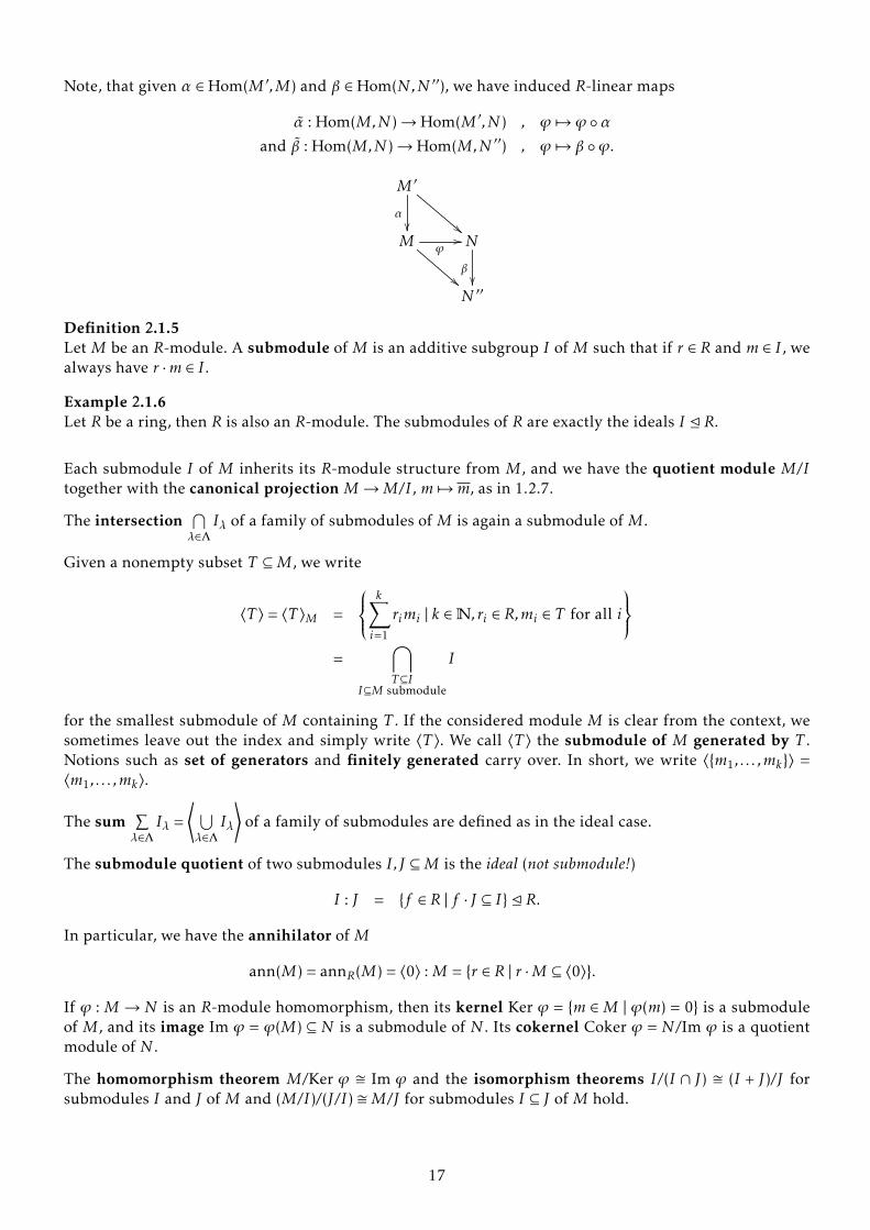
Note, that given α ∈Hom(M ′ ,M) and β ∈Hom(N,N ′′), we have induced R-linear maps

α : Hom(M,N )→Hom(M ′ ,N ) , ϕ 7→ ϕ ◦αand β : Hom(M,N )→Hom(M,N ′′) , ϕ 7→ β ◦ϕ.

M ′

""�M

""

ϕ// N

�

N ′′

Definition 2.1.5Let M be an R-module. A submodule of M is an additive subgroup I of M such that if r ∈ R and m ∈ I , wealways have r ·m ∈ I .

Example 2.1.6Let R be a ring, then R is also an R-module. The submodules of R are exactly the ideals I E R.

Each submodule I of M inherits its R-module structure from M, and we have the quotient module M/Itogether with the canonical projection M→M/I , m 7→m, as in 1.2.7.

The intersection⋂λ∈Λ

Iλ of a family of submodules of M is again a submodule of M.

Given a nonempty subset T ⊆M, we write

〈T 〉 = 〈T 〉M =

k∑i=1

rimi | k ∈N, ri ∈ R,mi ∈ T for all i

=

⋂T⊆I

I⊆M submodule

I

for the smallest submodule of M containing T . If the considered module M is clear from the context, wesometimes leave out the index and simply write 〈T 〉. We call 〈T 〉 the submodule of M generated by T .Notions such as set of generators and finitely generated carry over. In short, we write 〈{m1, . . . ,mk}〉 =〈m1, . . . ,mk〉.

The sum∑λ∈Λ

Iλ =⟨ ⋃λ∈Λ

Iλ

⟩of a family of submodules are defined as in the ideal case.

The submodule quotient of two submodules I, J ⊆M is the ideal (not submodule!)

I : J = {f ∈ R | f · J ⊆ I} E R.

In particular, we have the annihilator of M

ann(M) = annR(M) = 〈0〉 :M = {r ∈ R | r ·M ⊆ 〈0〉}.

If ϕ : M → N is an R-module homomorphism, then its kernel Ker ϕ = {m ∈M | ϕ(m) = 0} is a submoduleof M, and its image Im ϕ = ϕ(M) ⊆ N is a submodule of N . Its cokernel Coker ϕ = N/Im ϕ is a quotientmodule of N .

The homomorphism theorem M/Ker ϕ � Im ϕ and the isomorphism theorems I/(I ∩ J) � (I + J)/J forsubmodules I and J of M and (M/I)/(J/I) �M/J for submodules I ⊆ J of M hold.

17

Remark 2.1.7Let (Mλ)λ∈Λ be a family of R-modules, then componentwise operations make the sets∏

λ∈ΛMλ = {(mλ)λ∈Λ |mλ ∈Mλ for all λ ∈Λ}

and⊕λ∈Λ

Mλ = {(mλ)λ∈Λ ∈∏λ∈Λ

Mλ | only finitely many mλ are nonzero}

into R-modules. These are called the direct product respectively the direct sum of the Mλ, λ ∈Λ.

Finally, if I E R is an ideal and M is an R-module, then set

I ·M = 〈a ·m | a ∈ I,m ∈M〉M .

2.2 Free Modules

The perhaps most striking (and momentous) difference between modules over rings and vector space overfields is that modules in general lack the existence of a basis, i.e. a set of linearly independent generators.Compared with the linear algebra of vector spaces, this is a real catastrophe, since nearly everything thatmade vector spaces so likable is lost (at least on the first glance): All finitely dimensional K-vector spacesare isomorphic to Kn, linear maps between finitely dimensional vector spaces can be identified with ma-trices and so on. However, there are some modules that admit a basis, and we should honor them with anown name.

Definition 2.2.1Let R be a ring. A module F over R is called free if it is isomorphic to a direct sum of copies of R.

Equivalently, F admits a basis in the sense of linear algebra, i.e. there exists a set of R-linearly independentgenerators for F, a free basis. By convention, the zero-module is free.

Note that if F admits a finite free basis, its number of elements is independent of the choice of basis (wewill provide a proof in the next section). We call this number the rank of F, written rank F.

We think of every free R-module F of rank n < ∞ together with a fixed free basis as the free R-moduleRn = R× . . .×R︸ ︷︷ ︸

n times

with its canonical free basis e1 = (1,0, . . . ,0)T , . . . , en = (0, . . . ,0,1)T . Given two such modules

with fixed free bases, we regard each homomorphism between them as a matrix with entries in R. Thus,free modules behave in many ways very similar to vector spaces which of course makes them congenial,compared to arbitrary modules.

Example 2.2.2 (i) Let R be a ring and 〈0〉 , I E R an ideal. Then I is free if and only if I is a principleideal generated by a non-zero divisor. In fact, if n ≥ 2 and f1, . . . , fn ∈ I , then f1, . . . , fn are not R-linearlyindependent: fifj − fjfi = 0 for all i, j.

(ii) Let X be any set. The free abelian group on X is the free Z-module with free basis X. Its elementsare formal sums ∑

p∈Xnpp, np ∈Z, np = 0 for all but finitely many p.

The algebraic operation is formal addition∑p∈X

npp+∑p∈X

mpp =∑p∈X

(np +mp)p.

18

2.3 Finitely generated Modules, the Cayley-Hamilton Theorem and Nakayama’s Lemma

Note that an R-module M is finitely generated if and only if M is isomorphic to a quotient module of typeRn/I . Indeed, for M = 〈m1, . . . ,mn〉 consider the epimorphism

π : Rn→M , ei 7→mi .

By the homomorphism theorem, we get Rn/Ker π �M.

For the other direction, consider

π : Rn→ Rn/I�→M

and take mi = π(ei), which yields M = 〈m1, . . . ,mn〉 since π is surjective.

Theorem 2.3.1 (Cayley-Hamilton)Let R be a ring, I E R an ideal, M a finitely generated R-module and ϕ :M→M some homomorphism.

If M can be generated by n elements and if ϕ(M) ⊆ I ·M, then there exists a monic polynomial

χϕ(x) = xn + p1xn−1 + . . .+ pn ∈ R[x],

with pj ∈ I j = I · . . . · I︸ ︷︷ ︸j times

, such that

χϕ(ϕ) = 0 ∈Hom(M,M).

Proof. Let M = 〈m1, . . . ,mn〉R. Since ϕ(M) ⊆ I ·M, we may write each ϕ(mi) as an I-linear combination ofthe mj :

ϕ(mi) =n∑j=1

aijmj , with aij ∈ I . (∗)

We consider now M also as an R[x]-module via

x ·m = ϕ(m) for all m ∈M (∗∗)

and rewrite (∗) in matrix notation:

(x ·En −A)

m1...mn

=(xm1 −

∑aijmj

...

)(∗∗)=

0...0

,where A = (aij ) and En is the n×n identity matrix. Multiplying with the matrix of cofactors (x ·En −A)#, weget

det(xEn −A)

m1...mn

= 0.

So det(x ·En −A)mi = 0 ∀i, hence χϕ(x) := det(xEn −A) ∈ annR[x](M). By (∗∗), we have χϕ(ϕ) = 0. The resultfollows from the Leibniz rule for determinants.

Note that in general, an R-linear map ϕ : M → M may be injective without being bijective (even if it istempting to think so). As an easy counter-example, consider ϕ :Z→Z,n 7→ 2n. However, if ϕ is surjective,and M is finitely generated, we in fact can conclude bijectivity, as the following corollary states.

19

Corollary 2.3.2Let R be a ring and let M be a finitely generated R-module.

(i) If α ∈HomR(M,M) is surjective, then α is already bijective.

(ii) IfM � Rn, then any set of n elements generatingM is a free basis. In particular, rank M = n is well-defined.

Proof. (i) Suppose that α is surjective. We apply the theorem of Cayley-Hamilton to show that α has aninverse map. For this, consider M as R[t]–module via

t ·m := α(m) for all m ∈M.

Let I := 〈t〉 ⊆ R[t] , ϕ = idM ∈HomR[t](M,M).

Thenϕ(M) =M

α epi= α(M) = t ·M = I ·M .

Applying Cayley-Hamilton, we get a polynomial

χϕ(x) = xn +n−1∑i=0

pn−ixi ∈ R[t][x] ,

with pj ∈ 〈tj〉 for every j and

0 = χφ(ϕ) = idM +n−1∑i=0

Pn−i idM .

Now considerq(t) :=

p1 + . . .+ pnt

∈ R[t] .

Then, for all m ∈M,

m = idM(m) = (−n−1∑i=0

Pn−i idM(m)) = (−n−1∑i=0

Pn−i) ·m = t · (−q(t)) ·m

and, similarly, m = (−q(t)) · t ·m. This means that (α ◦ (−q(α)))(m) = (−q(α)) ◦ (α)(m). We conclude that−q(α) is inverse to α.

(ii) Fix an isomorphism β : M → Rn and suppose that M = 〈m1, . . . ,mn〉. Consider the epimorphism π :Rn → M,ei 7→ mi . Then π ◦ β : M → M is surjective and thus, an isomorphism by (i). Then alsoπ = (π ◦ β) ◦ β−1 is an isomorphism, hence m1, . . . ,mn are R–linearly independent:

0 =n∑i=1rimi ⇒ 0 =

n∑i=1riπ−1(mi) =

n∑i=1riei

⇒ ri = 0 ∀ i .

With regard to the rank, suppose that Rk � Rn, but n > k. Extend a free basis of length k by n−k zerosto a set of generators for M with n elements. Then this is not a free basis, a contradiction to the firststatement in (ii).

.

Corollary 2.3.3Let R be a ring, let M be a finitely generated R-module, and let I E R be an ideal such that I ·M =M. Then thereexists some r ∈ I such that

(1− r)M = 0.

20

Proof. Consider ϕ = idM in 2.3.1 to get pj ∈ I j ⊆ I such that1 +n−1∑i=0

pn−i

·m =

idM +n−1∑i=0

pn−i idM

(m)

= χϕ(ϕ)

= 0 for all m ∈M.

Now take r = −n−1∑i=0pn−i .

Corollary 2.3.4 (Nakayama’s Lemma)Let R be a ring, let M be a finitely generated R-module, and let I E R be an ideal contained in J(R). If I ·M =M,then M = 0.

Proof. Choose r ∈ I such that (1− r)M = 0 as in 2.3.3. Then r ∈m for all maximal ideals m E R since I ⊆ J(R)by assumption. Hence 1 − r < m (otherwise, 1 ∈ m) for all maximal ideals m of R, so that 1 − r ∈ R∗. Weconclude that M = 0.

The following local version of Nakayama’s Lemma is an extremely useful tool to study local rings.

Corollary 2.3.5 (Nakayama’s Lemma in Local Rings)Let (R,m) be a local ring, letM be a finitely generated R-module, and letN ⊆M be a submodule. IfN+m·M =M,then N =M.

Proof. Replace M by M/N to reduce to the case N = 〈0〉. If N = 〈0〉, the result follows from Nakayama’sLemma since m = J(R).

An important application of Nakayama’s Lemma is the following: We can thereby deduce information onfinitely generated modules over local rings from information on vector spaces.

Some notation: If M is an R-module, then a set of generators of M is called minimal if no proper subsetgenerates M.

Corollary 2.3.6Let (R,m) be a local ring, let M be a finitely generated R-module, and let m1, . . . ,mn ∈M. Then the mi generateM as an R-module if and only if the residue classes mi = mi +mM generate M/mM as an R/m-vector space. Inparticular, any minimal set of generators for M corresponds to an R/m-basis for M/mM and two such sets havethe same number of elements.

Proof. Let N = 〈m1, . . . ,mn〉. Then m1, . . . ,mn generate M(∗)⇔ N +mM =M, which in turn is equivalent to

spanR/m(m1, . . . ,mn) = M/mM.

Here, for the direction „⇐“ of (∗), we apply Nakayama’s Lemma for local rings.

Example 2.3.7The assertion of 2.3.6 may not hold in the non-local case: Consider a field K and

〈x,1 + x〉 = 〈1〉 = K[x]

(both sets of generators are minimal - but their number of elements is different).

Corollary 2.3.8Let (R,m) be a local ring, let M, N be finitely generated R-modules, and let ϕ : M → N be a homomorphism ofR-modules. Then ϕ is surjective if and only if the induced map ϕ :M/mM→N/mN,m 7→ ϕ(m) is surjective.

Proof. The direction „⇒“ is clear. For the converse direction, suppose ϕ is surjective. Then, given n ∈ N ,there is some m ∈M such that ϕ(m) = n. That is, ϕ(m)− n ∈mN . Hence, im ϕ +mN = N , so that im ϕ = Nby the local version of Nakayama’s Lemma.

21

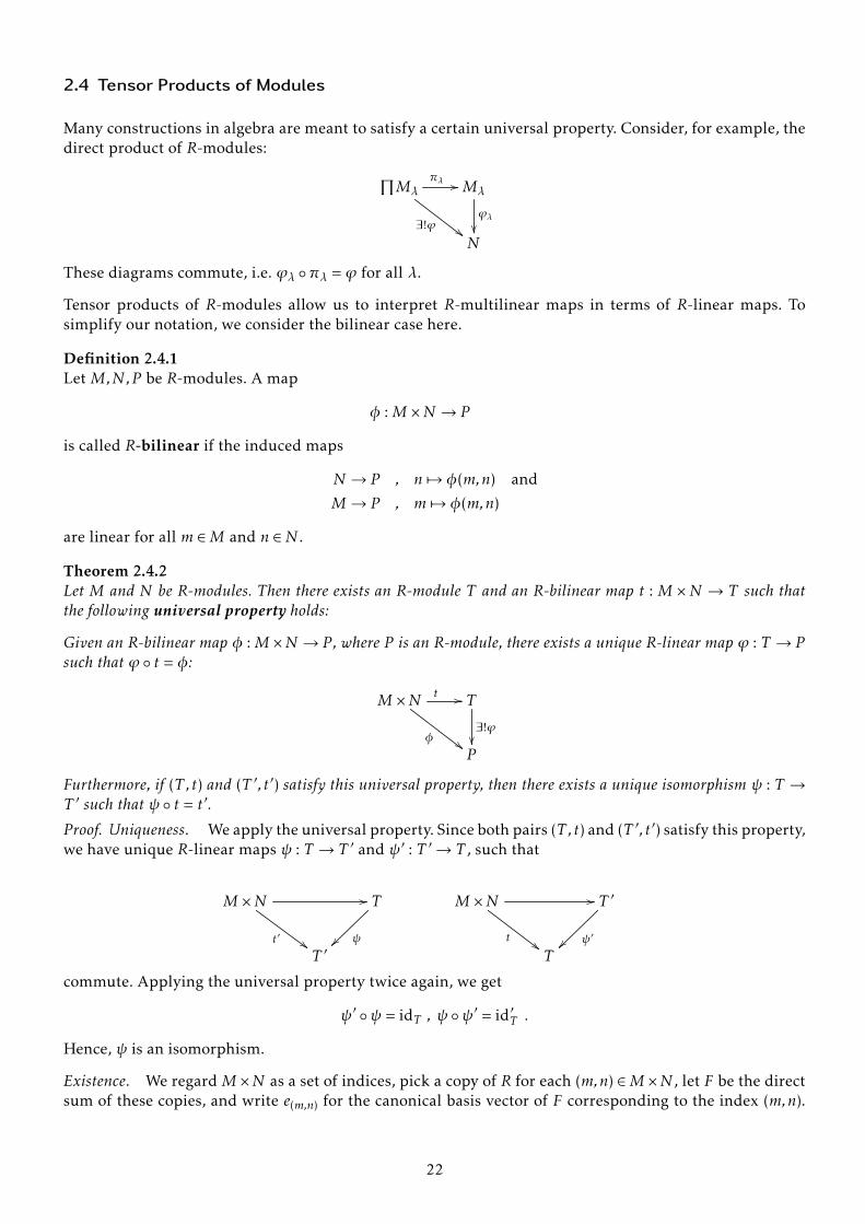
2.4 Tensor Products of Modules

Many constructions in algebra are meant to satisfy a certain universal property. Consider, for example, thedirect product of R-modules: ∏

Mλπλ //

∃!ϕ ##

Mλ

ϕλ��N

These diagrams commute, i.e. ϕλ ◦πλ = ϕ for all λ.

Tensor products of R-modules allow us to interpret R-multilinear maps in terms of R-linear maps. Tosimplify our notation, we consider the bilinear case here.

Definition 2.4.1Let M,N,P be R-modules. A map

φ :M ×N → P

is called R-bilinear if the induced maps

N → P , n 7→ φ(m,n) and

M→ P , m 7→ φ(m,n)

are linear for all m ∈M and n ∈N .

Theorem 2.4.2Let M and N be R-modules. Then there exists an R-module T and an R-bilinear map t : M ×N → T such thatthe following universal property holds:

Given an R-bilinear map φ :M ×N → P , where P is an R-module, there exists a unique R-linear map ϕ : T → Psuch that ϕ ◦ t = φ:

M ×N t //

φ ##

T

∃!ϕ��P

Furthermore, if (T ,t) and (T ′ , t′) satisfy this universal property, then there exists a unique isomorphism ψ : T →T ′ such that ψ ◦ t = t′.

Proof. Uniqueness. We apply the universal property. Since both pairs (T ,t) and (T ′ , t′) satisfy this property,we have unique R-linear maps ψ : T → T ′ and ψ′ : T ′→ T , such that

M ×N //

t′ ##

T

ψ~~T ′

M ×N //

t##

T ′

ψ′~~T

commute. Applying the universal property twice again, we get

ψ′ ◦ψ = idT , ψ ◦ψ′ = id′T .

Hence, ψ is an isomorphism.

Existence. We regard M ×N as a set of indices, pick a copy of R for each (m,n) ∈M ×N , let F be the directsum of these copies, and write e(m,n) for the canonical basis vector of F corresponding to the index (m,n).

22

Let I ⊂ F be the submodule generated by elements of the following types:

e(m+m′ ,n) − e(m,n) − e(m′ ,n)e(m,n+n′) − e(m.n) − e(m,n′)e(rm,n) − re(m,n)e(m,rn) − re(m,n)

where m,m′ ∈M, n,n′ ∈N, r ∈ R. Let T = F/I and consider the map t :M ×N → T , (m,n) 7→ e(m,n).

Then, by construction, t is R-bilinear.

Given an R-module P and an R-bilinear map φ :M ×N → P , consider the R-linear map

φ : F→ P ,e(m,n) 7→ φ(m,n).

Since φ is R–bilinear, φ vanishes on I and induces, thus, on R–linear map ϕ : T → P , such that ϕ ◦ t = φ.This condition determines ϕ.

Definition 2.4.3In the situation above, we call T the tensor product of M and N over R, written M ⊗N =M ⊗RN = T . Wealso write m⊗n = t(m,n).

Elements of M ⊗N of type m⊗n are also called pure tensors. Note that every element of M ⊗N is a finitesum of pure tensors:

Corollary 2.4.4Each w ∈M ⊗RN can be written as a sum of type

w =k∑i=1

mi ⊗ni ,

with mi ∈M, ni ∈N .

Proof. Use the notation of the previous proof. Let w = f ∈ F/I and write f as a (finite) R-linear combinationof the free basis vectors e(m,n).

Remark 2.4.5Given two setsX and Y of generators forM respectivelyN , the elements of type x⊗y (x ∈ X, y ∈ Y ) generateM ⊗N . In particular, if M and N are finitely generated, then so is M ⊗N .

From now on, we forget the construction of the tensor product and work with the universal property only.

Note that the tensor product M1 ⊗ · · · ⊗Mk of more than two R-modules is defined in the same way, askinga universal property for k-linear maps.

Proposition 2.4.6Let M,N,P be R-modules. Then there exist unique isomorphisms

(i) M ⊗N �N ⊗M,

(ii) (M ⊗N )⊗ P �M ⊗ (N ⊗ P ) �M ⊗N ⊗ P ,

(iii) (M ⊕N )⊗ P � (M ⊗ P )⊕ (N ⊗ P ),

(iv) R⊗M �M

such that

23

(i) m⊗n 7→ n⊗m,

(ii) (m⊗n)⊗ p 7→m⊗ (n⊗ p) 7→m⊗n⊗ p,

(iii) (m,n)⊗ p 7→ (m⊗ p,n⊗ p),

(iv) r ⊗m 7→ r ·m.

Proof. We apply the universal property. Let us for example show (iii): The map

(M ⊕N )× P → (M ⊗ P )⊕ (N ⊗ P ),

((m,n),p) 7→ (m⊗ p,n⊗ p)

is R-bilinear in (m,n) and p. Hence we have an R-linear map

ϕ : (M ⊕N )⊗ P → (M ⊗ P )⊕ (N ⊗ P ) such that

(m,n)⊗ p 7→ (m⊗ p,n⊗ p).

The converse map is constructed in the same way: From the universal property we get R-linear mapsM ⊗ P → (M ⊕N )⊗ P and N ⊗ P → (M ⊕N )⊗ P which add up to an R-linear map

ψ : (M ⊗ P )⊕ (N ⊗ P )→ (M ⊕N )⊗ P such that (m⊗ p,n⊗ q) 7→ (m,0)⊗ p+ (0,n)⊗ q.

Clearly, ϕ and ψ are inverse to each other (it is enough, to check this on pure tensors).

Similar arguments give us the following examples (see exercises):

Example 2.4.7 (i) We have isomorphisms

Rm ⊗ Rn�−→ Mat(m×n,R) such that

x1...xm

⊗y1...yn

7→ (xi · yj ).

In particular, the ei ⊗ ej form a free basis for Rm ⊗Rn.

(ii) Let M be an R-module and let I E R be an ideal. Then we have an isomorphism

M ⊗R/I �−→ M/IM such that

m⊗ r 7−→ rm.

(iii) If M,N,P are R-modules, then we have an isomorphism

HomR(M ⊗N,P )�−→ HomR(M,HomR(N,P )) such that

ϕ�7−→ ϕ :M→HomR(N,P ),

m 7→ (N → P ,n 7→ ϕ(m⊗n)).

Remark 2.4.8If ϕ :M→N and ϕ′ :M ′→N ′ are R-linear maps, then

M ×M ′→N ⊗N ′ , (m,m′) 7→ ϕ(m)⊗ϕ′(m′)

is R-bilinear. Hence, we have a homomorphism

ϕ ⊗ϕ′ :M ⊗M ′ → N ⊗N ′ such that

m⊗m′ 7→ ϕ(m)⊗ϕ′(m′).

24

2.5 R-algebras

Given a homomorphism ϕ : R→ S of rings, we make S into an R-module by setting

r · s = ϕ(r) · s for all r ∈ R, s ∈ S.

Then the R-module structure is compatible with the ring structure on S, that is (r · s) · s′ = r · (s · s′) for allr ∈ R, s, s′ ∈ S.

We call the ring S together with the above R-module structure an R-algebra. A subalgebra of S is a subringS ′ ⊆ S containing im ϕ.

Example 2.5.1If R = K is a field, S , 0 is a ring, and ϕ : K → S is a ring homomorphism (in particular ϕ(1K ) = 1S ), thenϕ is a monomorphism. Identifying K with its image in S, we see that a K-algebra is nothing but a ring Scontaining K as a subring.

For instance, K[x1, . . . ,xn] contains K as the subring of constant polynomials.

An R-algebra homomorphism between two R-algebras S and T is a ring homomorphism α : S→ T whichis also an R-module homomorphism. In terms of ring homomorphisms ϕ : R→ S and ψ : R→ T definingthe R-algebra structures, this means α ◦ϕ = ψ.

Example 2.5.2 (Tensor Product of R-algebras)Let S,T be R-algebras, defined by homomorphisms ϕ : R→ S and ψ : R→ T . Then the universal propertyof the multilinear tensor product and 2.4.6 yield a multiplication on S ⊗R T such that

(s⊗ t)(s′ ⊗ t′) = ss′ ⊗ tt′.

This gives a ring with unity 1S ⊗ 1T , which is actually an R-algebra: We have the ring homomorphism

R→ S ⊗R T , r 7→ ϕ(r)⊗ψ(r).

2.6 Exact sequences

Let R be any ring.

Definition 2.6.1A complex of R-modules is a finite or infinite sequence of R-modules and homomorphisms of R-modules

. . .→Mi+1ϕi+1→ Mi

ϕi→Mi−1→ . . .

such that ϕi ◦ϕi+1 = 0.

The homology of the complex at Mi is ker ϕi/im ϕi+1. We call the complex exact at Mi if the homology atMi is zero, i.e. if im ϕi+1 = ker ϕi . We call the whole complex exact if it is exact at each Mi .

Note that a finite sequence Mr →Mr−1→ . . .→Ms+1→Ms is exact if and only if it is exact at each Mi fori = r − 1, . . . , s+ 1.

Example 2.6.2Let ϕ : M → N be an R-linear map. We write 0 for the zero-module and 0→ M and N → 0 for the zerohomomorphisms. Then it holds:

25

(i) ϕ is injective⇔ 0→Mϕ→N is exact

(ii) ϕ is surjective⇔Mϕ→N → 0 is exact

(iii) ϕ is bijective⇔ 0→Mϕ→N → 0 is exact

Example 2.6.3A short exact sequence is an exact sequence of the following type:

0→M ′ϕ→M

ψ→M ′′→ 0.

That is, ϕ is injective, ψ is surjective, and im ϕ = ker ψ.

For instance, given an R-module M and a submodule N ⊆M, we have a short exact sequence

0→Nϕ→M

ψ→M/N → 0,

where ϕ in the inclusion and ψ is the projection.

Given an R-linear map ϕ :M→N , the sequence

0→ ker ϕ→M→ im ϕ→ 0

is short exact.

Note that a sequence

. . .→Mi+1ϕi+1→ Mi

ϕi→Mi−1→ . . .

as in 2.6.1 is exact if and only if each induced sequence

0→Mi+1/ker ϕi+1→Mi → im ϕi → 0

is short exact (note also that Mi+1/Ker ϕi+1 � Im ϕi+1 by the homomorphism theorem).

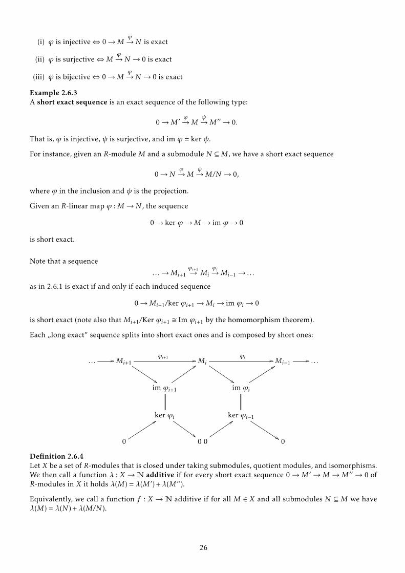
Each „long exact“ sequence splits into short exact ones and is composed by short ones:

. . . //Mi+1

$$

ϕi+1 //Mi

$$

ϕi //Mi−1// . . .

im ϕi+1

::

im ϕi

99

ker ϕi

$$

ker ϕi−1

%%0

99

0 0

::

0

Definition 2.6.4Let X be a set of R-modules that is closed under taking submodules, quotient modules, and isomorphisms.We then call a function λ : X →N additive if for every short exact sequence 0→M ′ →M →M ′′ → 0 ofR-modules in X it holds λ(M) = λ(M ′) +λ(M ′′).

Equivalently, we call a function f : X →N additive if for all M ∈ X and all submodules N ⊆M we haveλ(M) = λ(N ) +λ(M/N ).

26

Example 2.6.5If R = K is a field and X the set of all finitely generated K-vector spaces, then the dimension dimK is anadditive function X→N. In fact, this very example is the motivation for the above definition.

Proposition 2.6.6

Let λ : X →N be an additive function and let 0→Mrϕr→Mr−1→ . . .→Ms+1

ϕs+1→ Ms→ 0 be an exact sequenceof R-modules in X. Then it holds

r∑i=s

(−1)i ·λ(Mi) = 0.

Proof. Cut the sequence into short exact sequences.

Complexes and exact sequences are studied in further detail in Homological Algebra. In this course, theywill serve as a useful universal tool which will make life easier for us in most of the following chapters,for example in some proofs. Therefor, it makes sense to have another look (maybe more than one) at exactsequences at this place.

Lemma 2.6.7 (5-Lemma)Let

M5ϕ5 //

α1

��

M4ϕ4 //

β1��

M3ϕ3 //

γ

��

M2ϕ2 //

β2��

M1

α2

��N5 ψ5

// N4 ψ4

// N3 ψ3

// N2 ψ2

// N1

be a commutative diagram of R-modules with exact rows. Suppose β1 and β2 are both isomorphisms, that α1 isan epimorphism and that α2 is a monomorphism.

Then γ is an isomorphism.

Proof. By chasing the diagram.

Show: γ injective.

m3 ∈M3, γ(m3) = 0 =⇒commutativity

(β2 ◦ϕ3)(m3) = (ψ3 ◦γ)(m3) = 0

⇒β2 mono

ϕ3(m3) = 0

=⇒exactness

∃ m4 ∈M4 : ϕ4(m4) =m3

=⇒commutativity

(ψ4 ◦ β1) (m4) = (γ ◦ϕ4)(m4) = 0

=⇒exactness

∃ n5 ∈N5 : ψ5(n5) = β1(m4)

=⇒α1 epi

∃ m5 ∈M5 : α1(m5) = n5

=⇒commutativity, β1 mono

ϕ5(m5) =m4

=⇒exactness

m3 = (ϕ4 ◦ϕ5)(m5) = 0.

27

Show: γ is surjective.

n3 ∈N3 =⇒β2 epi

∃ m2 ∈M2 : β2(m2) = ψ3(n3)

=⇒commutativity, exactness

(α2 ◦ϕ2)(m2) = (ψ2 ◦ β2(m2) = (ψ2 ◦ψ3)(n3) = 0

=⇒α2 mono

ϕ2(m2) = 0

=⇒exactness

∃m′3 ∈M3 : ϕ3(m′3) =m2 ; n′3 := γ(m′3)

=⇒commutativity

ψ3(n3 −n′3) = β2(m2)− β2(m2) = 0

=⇒exactness

∃ n4 ∈N4 : ψ4(n4) = n3 −n′3=⇒β1 epi

∃ m4 ∈M4 : β1(m4) = n4 ; m3 := ϕ4(m4) +m′3

=⇒commutativity

γ(m3) = (γ ◦ϕ4)(m4) +γ(m′3) = (ψ4 ◦ β1)(m4) +n′3 = ψ4(n4) +n′3

= n3 −n′3 +n′3 = n3.

Corollary 2.6.8

For a short exact sequence 0→M ′ϕ→M

ψ→M ′′→ 0 there are equivalent:

(i) There exists α ∈Hom(M ′′ ,M) such that ψ ◦α = idM ′′ .

(ii) There exists β ∈Hom(M,M ′) such that β ◦ϕ = idM ′ .

If these conditions are fulfilled, then M �M ′ ⊕M ′′ and we call the sequence split-exact.

Proof. (i)⇒ (ii): Consider the commutative diagram

m′ // (m′ ,0), (m′ ,m′′) // m′′

0 //M ′

=��

//M ′ ⊕M ′′

ϕ+α��

//M ′′

=��

// 0

0 //M ′ϕ //M

ψ //M ′′ // 0

with exact rows. Then ϕ +α is an isomorphism by the 5-lemma.

Now take β = πM ′ ◦ (ϕ +α)−1, where πM ′ is the projection M ′ ⊕M ′′→M ′.

(ii)⇒ (i): Consider similarly the diagram

0 //M ′

=��

ϕ //M

(β,ψ)��

ψ //M ′′

=��

// 0

0 //M ′ //M ′ ⊕M ′′ //M ′′ // 0

and take α(m′′) = (β,ψ)−1(0,m′′) .

We now study exactness properties of Hom and ⊗.

Proposition 2.6.9Consider R-modules M ′ ,M,M ′′ ,N and R-linear maps ϕ :M ′→M, ψ :M→M ′′.

(i) The sequence M ′ϕ→M

ψ→M ′′→ 0 is exact if and only if the induced sequence

0→Hom(M ′′ ,N )→Hom(M,N )→Hom(M ′ ,N )

is exact.

28

(ii) The sequence 0→M ′ϕ→M

ψ→M ′′ is exact if and only if the induced sequence

0→Hom(N,M ′)→Hom(N,M)→Hom(N,M ′′)

is exact.Proof. Exercise.

Proposition 2.6.10

With notation as above, we have: If M ′ϕ→M

ψ→M ′′→ 0 is exact, then also

M ′ ⊗Nϕ⊗idN−→ M ⊗N

ψ⊗idN−→ M ′′ ⊗N → 0

is exact.Proof. If M ′→M→M ′′→ 0 is exact, then

0→Hom(M ′′ ,Hom(N,P ))→Hom(M,Hom(N,P ))→Hom(M ′ ,Hom(N,P ))

is exact by 2.6.9, (i) (consider any R-module P ). Hence, by 2.4.7, (iii) the sequence

0→Hom(M ′′ ⊗N,P )→Hom(M ⊗N,P )→Hom(M ′ ⊗N,P )

is exact. The result follows by using again 2.6.9, (i).

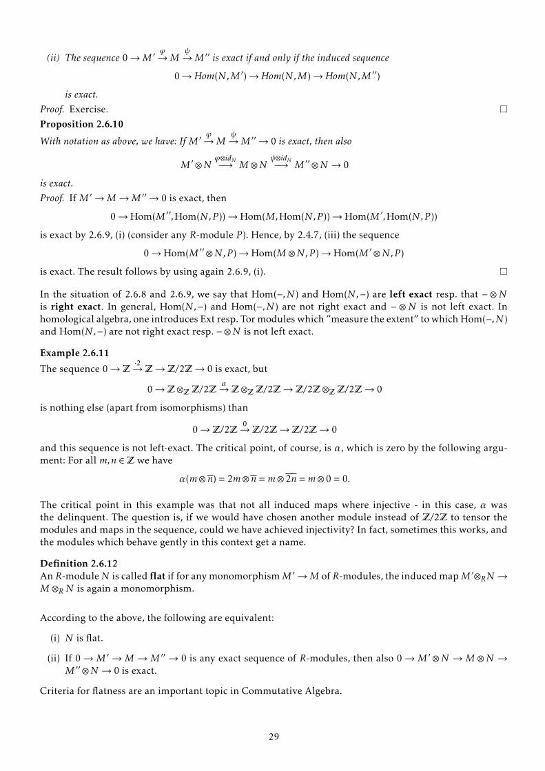
In the situation of 2.6.8 and 2.6.9, we say that Hom(−,N ) and Hom(N,−) are left exact resp. that − ⊗Nis right exact. In general, Hom(N,−) and Hom(−,N ) are not right exact and − ⊗ N is not left exact. Inhomological algebra, one introduces Ext resp. Tor modules which ”measure the extent” to which Hom(−,N )and Hom(N,−) are not right exact resp. −⊗N is not left exact.

Example 2.6.11

The sequence 0→Z

·2→Z→Z/2Z→ 0 is exact, but

0→Z⊗ZZ/2Z

α→Z⊗ZZ/2Z→Z/2Z⊗

ZZ/2Z→ 0

is nothing else (apart from isomorphisms) than

0→Z/2Z0→Z/2Z→Z/2Z→ 0

and this sequence is not left-exact. The critical point, of course, is α, which is zero by the following argu-ment: For all m,n ∈Z we have

α(m⊗n) = 2m⊗n =m⊗ 2n =m⊗ 0 = 0.

The critical point in this example was that not all induced maps where injective - in this case, α wasthe delinquent. The question is, if we would have chosen another module instead of Z/2Z to tensor themodules and maps in the sequence, could we have achieved injectivity? In fact, sometimes this works, andthe modules which behave gently in this context get a name.

Definition 2.6.12AnR-moduleN is called flat if for any monomorphismM ′→M ofR-modules, the induced mapM ′⊗RN →M ⊗RN is again a monomorphism.

According to the above, the following are equivalent:

(i) N is flat.

(ii) If 0→M ′ →M →M ′′ → 0 is any exact sequence of R-modules, then also 0→M ′ ⊗N →M ⊗N →M ′′ ⊗N → 0 is exact.

Criteria for flatness are an important topic in Commutative Algebra.

29

3 Localization

3.1 Localization of Rings

Constructing the rational numbers Q from the integers Z means to invert all integers different from zero.Formally, set U =Z \ {0} and define an equivalence relation on Z×U by

(r,u) ∼ (r ′ ,u′) ⇔ r ′u − ru′ = 0.

We write ru for the equivalence class of (r,u) and set Q = { ru | (r,u) ∈ Z ×U }. Of course, we define addi-

tion and multiplication in the usual way. Given any integral domain R, the same construction yields thequotient field Q(R).

Of course, we might consider other subsets U of R than just R \ {0} as we did above. However, we shouldmake sure that the construction we thereby get behaves reasonably.

Definition 3.1.1A subset U of a ring R is called multiplicatively closed, if 1 ∈ U and the product of any two elements ofU is again contained in U .

In general, when inverting elements of a ring, the product of two inverted elements is an inverse to theproduct. Thus, according to the above, it makes sense to invert elements from multiplicatively closed sub-sets.

In the presence of zero-divisors, the definition of the equivalence relation requires some care.

Definition 3.1.2Let R be a ring and U ⊆ R a multiplicatively closed subset. We define an equivalence relation on R×U by

(r,u) ∼ (r ′ ,u′) ⇔ v(r ′u − ru′) = 0 for some v ∈U .

We write ru for the equivalence class of (r,u) ∈ R×U and R[U−1] = U−1R = { ru | (r,u) ∈ R×U } for the set of

equivalence classes. To turn R[U−1] into a ring, we define addition and multiplication by

ru

+r ′

u′=

ru′ + r ′uuu′

,

ru· r′

u′=

rr ′

uu′.

Call this ring the localization of R at U .

Note that the element v ∈U in the definition is needed to guarantee transitivity of ∼.

We have a natural ring homomorphism ι : R→ R[U−1], r 7→ r1 . It holds true:

• ι sends elements of U to units in R[U−1].

• ι sends r ∈ R to 0 if and only if there exists some v ∈ U such that v · r = 0. In particular, ι is injectiveexactly if U does not contain a zero-divisor.

• We have R[U−1] = 0 if and only if 0 ∈U .

Proposition 3.1.3 (Universal property of Localization)Let R be a ring and let U ⊆ R be a multiplicatively closed subset. If ϕ : R→ S is a homomorphism of rings whichmaps elements of U to units in S, then there exists a unique homomorphism Φ : R[U−1]→ S such that

30

Rϕ //

ι ""

S

R[U−1]Φ

<<

commutes.

Proof. We will separately prove the existence and the uniqueness of such a homomorphism Φ .

Uniqueness Suppose Φ satisfies the condition. Then Φ( r1 ) = (Φ ◦ ι(r)) = ϕ(r) for all r ∈ R. Hence, Φ( 1u ) =

Φ((u1 )−1

)= Φ(u1 )−1 = ϕ(u)−1 for all u ∈U .

It follows that Φ is determined by ϕ since

Φ

( ru

)= Φ

( r1

)·Φ

(1u

)= ϕ(r) ·ϕ(u)−1 for all r ∈ R,u ∈U .

Existence Let Φ( ru ) := ϕ(r)ϕ(u)−1 ∀r ∈ R,u ∈U .

Then Φ is a ring homomorphism as desired, provided it is well–defined.

For the latter, let ru = r ′

u′ ∈ R[u−1]. Then ∃ v ∈U such that v(ru′ − r ′u) = 0. Consequently

ϕ(v)(ϕ(r)ϕ(u′)−ϕ(r ′)ϕ(u)) = 0.

Since ϕ(v) is a unit in S by assumption, we have

ϕ(r)ϕ(u)−1 = ϕ(r ′)ϕ(u′)−1.

Remark 3.1.4Using the notation of 1.2.10 we have extensions and contractions with respect to ι:

• If I ⊆ R is an ideal, thenIe = 〈ι(I)〉 =

{ ru

∣∣∣ r ∈ I,u ∈U }⊆ R[U−1]

is the extension of I to R[U−1]. Indeed, given∑i

riuiai1 ∈ I

e, with all ri ∈ R,ui ∈ U,ai ∈ I , we can bring

this sum to a common denominator, which gives one inclusion. The other inclusion is clear.

• If J E R[U−1] is an ideal, thenJc = ι−1(J) =

{r ∈ R

∣∣∣ r1∈ J

}⊆ R

is the contraction of J to R.

In the following, we will examine the ideal theory of R[U−1] and, hopefully, will see that it is simpler thanthat of R. This gives us a justification for the construction of localization, apart from just being interestedin new structures.

Theorem 3.1.5LetR be a ring, letU ⊆ R be a multiplicatively closed subset, and let ι : R→ R[U−1] be the natural homomorphism.

(i) If I E R is an ideal, then

Iec = {r ∈ R | vr ∈ I for some v ∈U }.

(ii) If J E R[U−1] is an ideal, then

Jce = J .

We thus get an injective map of the set of ideals of R[U−1] into the set of ideals of R by sending J to Jc.

31

(iii) The injection J 7→ Jc restricts to a bijection between the set of prime ideals of R[U−1] and the set of primeideals of R which do not meet U (i.e. which are disjoint with U ).

Proof. (i) Let r ∈ R. Then:

r ∈ Iec ⇐⇒ r1∈ Ie

3.1.4⇐⇒ r

1=su

for some s ∈ I, u ∈U

⇐⇒ vr ∈ I for some v ∈U .

(ii) By 1.2.11, (i), we have Jce ⊆ J . For the converse inclusion, let r ∈ R, u ∈U . Then

ru∈ J =⇒ r

1∈ J =⇒ r ∈ Jc =⇒ r

u∈ Jce.

(iii) Let Q E R[U−1] be a prime ideal. Then P = ι−1(Q) E R is a prime ideal. Furthermore, P ∩U = ∅ sinceQ does not contain units.

Conversely, let P E R be a prime ideal such that P ∩U = ∅. Then 1 < P e since 1 < P , so P e is a properideal of R[U−1]. If r

u ·sv ∈ P

e with u,v ∈ U , then wrs ∈ P for some w ∈ U by 3.1.4. Then w < P sinceP ∩U = ∅ and hence we have r ∈ P or s ∈ P because P is a prime ideal. But this means r

u ∈ Pe or s

v ∈ Pe,

and hence P e is a prime ideal. Furthermore, by (i) we have P ec = {r ∈ R | wr ∈ P for some w ∈ U } = P .Taking (ii) into account, we conclude that Q 7→Qc is a bijective map on the set of prime ideals.

Example 3.1.6Let R be a ring.

(i) Consider the set U of all non-zero-divisors of R. Then we call Q(R) = R[U−1] the total quotient ringof R. In the special case where R is an integral domain, Q(R) is a field, the quotient field of R.

(ii) Let f ∈ R and let U = {f m |m ≥ 0}. Then we write Rf = R[U−1] = R[ 1f ].

(iii) If P E R is a prime ideal and U = R \ P , then we call RP = R[U−1] the localization of R at P . Note thatRP is a local ring with maximal ideal

m = P e ={ ru

∣∣∣ r ∈ P ,u ∈U = R \ P}

.

Indeed, if ru ∈ RP \m, then r ∈ R \ P , so r

u is a unit in RP . Hence, RP \m = R∗P , which means that m isthe unique maximal ideal of RP .

The localization at prime ideals is of great importance in commutative algebra as well as in algebraicgeometry where the localization at prime ideals plays a central role in the local study of zero sets of poly-nomials. This is why we speak of local rings and localization.

Example 3.1.7By inverting all elements in Z \ {0}, we get Q, as we already know. By inverting fewer elements, we getsubrings of Q. For instance, if n ∈Z \ {0}, we get

Z

[1n

]=

{ab∈Q

∣∣∣ b = nk for some k ∈N}

or, if p ∈Z is a prime number, we get

Z〈p〉 ={ab∈Q

∣∣∣ p does not divide b}

.

If p does not divide n, we have the inclusions of rings

Z ⊆ Z

[1n

]⊆ Z〈p〉 ⊆ Q.

32

3.2 Localization of Modules

By essentially the same construction as for rings, we also can define localizations for modules. As each ringis a module over itself, this is just an obvious generalization.

Definition 3.2.1Let R be a ring, let U ⊆ R be some multiplicatively closed subset, and let M be an R-module. We get anequivalence relation on M ×U by setting

(m,u) ∼ (m′ ,u′) ⇔ v(u′m−um′) = 0 for some v ∈U .

We write M[U−1] =U−1M = {mu |m ∈M,u ∈U } for the set of equivalence classes and make M[U−1] into anR[U−1]-module, with addition as for R[U−1], and scalar multiplication r

u ·mu′ = r·m

u·u′ .

This module is called the localization of M at U .

Remark 3.2.2For a ring R and an R-module homomorphism ϕ :M→N , we have an induced homomorphism

ϕ[U−1] : M[U−1] → N [U−1],mu7→

ϕ(m)u

of R[U−1]-modules.

Localization at U is a covariant functor in the sense of the following functor properties:

(i) idM [U−1] = idM[U−1]

(ii) If M ′ϕ−→M

ψ−→M ′′ are homomorphisms of R-modules, then (ψ ◦ϕ)[U−1] = ψ[U−1] ◦ϕ[U−1].

Remark 3.2.3Let R be a ring, let I E R be an ideal, and let U ⊆ R be multiplicatively closed. Then

Ie = I[U−1].

This is clear because of 3.1.4.

Proposition 3.2.4

If M ′ϕ−→M

ψ−→M ′′ is an exact sequence of R-modules, then M ′[U−1]

ϕ[U−1]−→ M[U−1]

ψ[U−1]−→ M ′′[U−1] is an exact

sequence of R[U−1]-modules.

We say that localization at U is an exact functor.

Proof. We know that

ψ[U−1] ◦ϕ[U−1] = (ψ ◦ϕ)[U−1] = 0,

so im ϕ[U−1] ⊆ ker ψ[U−1]. We now show the other inclusion. Let mu ∈ ker ψ[U−1]. Then

0 = ψ[U−1](mu

)=

ψ(m)u

.

Hence, there is some v ∈ U such that v ·ψ(m) = 0, so ψ(v ·m) = 0. But then v ·m ∈ ker ψ = im ϕ. By this,there exists m′ ∈M ′ with ϕ(m′) = v ·m.

33

Now we can finally conclude that

mu

=vmvu

=ϕ(m′)vu

= ϕ[U−1](m′

vu

)∈ im ϕ[U−1]

which proves ker ψ[U−1] ⊆ im ϕ[U−1].

The proposition implies in particular that if N is a submodule of M, then the map N [U−1] → M[U−1]induced by the inclusion is a monomorphism. We may thus regard N [U−1] as a submodule of M[U−1].

Let us examine the behavior of localization when it comes to certain operations on modules, like sum orintersection or factor structures. Luckily, there is nothing to worry about, everything works just as fine asit could.

Corollary 3.2.5If N and P are submodules of an R-module M, then it holds

(i) (N + P )[U−1] =N [U−1] + P [U−1],

(ii) (N ∩ P )[U−1] =N [U−1]∩ P [U−1],

(iii) (M/N )[U−1] �M[U−1]/N [U−1].

Proof. (i) is immediate from the definitions.

(ii) Clearly, (N ∩ P )[U−1] ⊆N [U−1]∩ P [U−1].

For the other inclusion, let yu = z

v ∈ N [U−1]∩ P [U−1], with y ∈ N , z ∈ P , u,v ∈ U . Then there existsw ∈U such that w(vy − zu) = 0, so that w′ := wvy︸︷︷︸

∈N

= wzu︸︷︷︸∈P

∈N ∩ P and, thus,

y

u=

w′

uvw∈ (N ∩ P )[U−1].

This shows that (N ∩ P )[U−1] ⊇N [U−1]∩ P [U−1].

(iii) By 3.2.4, since the sequence 0→N →M→M/N → 0 is exact, the sequence

0→N [U−1]→M[U−1]→ (M/N )[U−1]→ 0

is exact, too. Hence, (M/N )[U−1] �M[U−1]/N [U−1].

Proposition 3.2.6Let M be an R-module. Then the R[U−1]-modules M[U−1] and R[U−1] ⊗RM are isomorphic. More precisely,there exists a unique isomorphism

ϕ : R[U−1]⊗RM → M[U−1] such thatru⊗m 7→ rm

u.

Proof. Since the map R[U−1]×M→M[U−1], ( ru ,m) 7→ rmu is bilinear, there exists a unique homomorphism

ϕ sending ru ⊗m to rm

u . This homomorphism is clearly surjective.

We show that ϕ is also injective. For this, let∑i

riui⊗mi ∈ R[U−1] ⊗RM be any element. Set u :=

∏iui ∈

U , vi :=∏j,iuj . Then we get:

∑i

riui⊗mi =

∑i

riviu ⊗mi =

∑i

1u ⊗ rivimi = 1

u ⊗∑irivimi . It follows that any element

of R[U−1]⊗M is of the form 1u ⊗m for some u ∈U and m ∈M.

Now suppose that ϕ( 1u ⊗m) = 0. That is, suppose that m

u = 0. Then ∃ v ∈U such that vm = 0. Hence,

1u⊗m =

vuv⊗m =

1uv⊗ vm =

1uv⊗ 0 = 0 .

34

Note that in the proposition above, we consider R[U−1] as an R-module via ι : R→ R[U−1] as in Section 2.5.

Corollary 3.2.7R[U−1] is a flat R-module.

Proof. This follows from 3.2.6 and 3.2.4.

Proposition 3.2.8If M and N are R-modules, then there exists a unique isomorphism of R[U−1]-modules

ϕ : M[U−1]⊗R[U−1]N [U−1] → (M ⊗RN )[U−1] such thatmu⊗ nv7→ m⊗n

u · v.

Proof. This follows from 3.2.6, using the canonical isomorphism in 2.4.6, (iv).

IfM is an R-module, P ⊆ R is a prime ideal, and U = R\P , then we also writeMP =M[U−1]. If N is anotherR-module, we conclude from the proposition that

MP ⊗RP NP � (M ⊗RN )P

as RP -modules.

3.3 Local Properties

We study properties of a module M over a ring R which are local in the sense that M has this property ifand only if MP has the property for all prime ideals P of R.

This makes localization a powerful tool by which we can translate a (possibly hard) problem into a localversion, which is sometimes easier to solve in the „local world“, and afterwards translate the result backinto the „global world“.

The first local property we encounter here is „being zero“:

Proposition 3.3.1If M is an R-module, then the following are equivalent:

(i) M = 0.

(ii) MP = 0 for all prime ideals P E R.

(iii) Mm = 0 for all maximal ideals m E R.

Proof. The implications (i)⇒ (ii) and (ii)⇒ (iii) are obvious (note for the latter that every maximal ideal isalso a prime ideal). So the only interesting part is (iii)⇒ (i). Let us prove it by contraposition: „not (i)“⇒„not (iii)“.

Suppose M , 0 and let m ∈ M be nonzero. Then the annihilator ann(m) is a proper ideal of R (indeed,ann(m) cannot be the whole ring since e.g. 1 is not contained). Thus, there exists a maximal ideal m of Rsuch that ann(m) ⊆m.

But then, the element m1 ∈Mm is nonzero since otherwise there would exist some u ∈ R\m such that um = 0.This u would thus be contained in the annihilator of m, but this is a subset of m – Contradiction!

Hence, Mm , 0, which completes the proof since we found a nonzero localization at a maximal ideal.

The next local property is injectivity of homomorphisms.

Proposition 3.3.2Let M,N be R-modules and let ϕ :M→N be a homomorphism. Then the following are equivalent:

35

(i) ϕ is injective.

(ii) ϕP :MP →NP is injective for all prime ideals P E R.

(iii) ϕm :Mm→Nm is injective for all maximal ideals m E R.

Proof. As in the preceding proposition, the proof will be rather short when it comes to the two first impli-cations. Nevertheless, some argument is needed at least in the first.

(i)⇒ (ii) That ϕ is injective means that 0→M → N is an exact sequence. By 3.2.4, if P E R is any primeideal, the sequence 0→MP →NP is exact as well. This, in turn, means that ϕP is injective.

(ii)⇒ (iii) is clear.

(iii)⇒ (i) Consider the exact sequence

0→ Ker ϕ→Mϕ→N.

Then by 3.2.4, for all maximal ideals m of R, we get the exact sequence

0→ (Ker ϕ)m→Mm

ϕm→ Nm.

If (iii) holds, then all kernels (Ker ϕ)m are zero, so that also Ker ϕ = 0 by 3.3.1 („being zero“ is a localproperty as we just proved above). But this mean nothing else than ϕ is injective.

Remark 3.3.3The assertion of Proposition 3.3.2 also holds if we replace “injective” by “surjective” (resp. “bijective”) inall statements (the proof is analogous).

Leaving the proof as an exercise, we mention that flatness is a local property:

Proposition 3.3.4For any R-module M, the following are equivalent:

(i) M is a flat R-module.

(ii) MP is a flat RP -module for all prime ideals P E R.

(iii) Mm is a flat Rm-module for all maximal ideals m E R.

Proof. Exercise.

36

4 Chain Conditions

4.1 Noetherian Rings and Modules

We study rings (modules) in which every ideal (submodule) is finitely generated. Rings of the desired typeare characterized by an important criterion by Emmy Noether.

Theorem 4.1.1For a ring R, the following are equivalent:

(i) Finiteness condition: Every ideal of R is finitely generated.

(ii) Ascending Chain Condition: Every chain I1 ⊂ I2 ⊂ . . . of ideals in R is eventually stationary, i.e. Im =Im+1 = . . . for some m ≥ 1.

(iii) Maximal condition: Every nonempty set of ideals of R has a maximal element with respect to inclusion.

Proof. (i)⇒ (ii) Let I1 ⊆ I2 ⊆ . . . be an ascending chain of ideals in R. Then⋃jIj is an ideal as well. By (i),

this ideal is finitely generated, say⋃jIj = 〈a1, . . . , an〉. Then ∃ m ∈ N such that Im contains all ai . It

follows that Im = Im+1 = . . ..

(ii)⇒ (iii) Let Γ be a nonempty set of ideals in R. Choose I1 ∈ Γ . If I1 is not maximal in Γ , ∃ I2 ∈ Γ such thatI1 ( I2. By (ii), this process has to stop after finitely many steps. Hence, Γ admits a maximal element.

(iii)⇒ (i) Let I be an ideal of R. Let Γ be the set of all ideals in R generated by a finite subset of I . Then Γ is anonempty set of ideals in R (for example, 〈0〉 ∈ Γ ). By (iii), Γ has a maximal element J = 〈a1, . . . , an〉 ⊂ I .Now let r ∈ I . Then, by the choice of J , we have J = 〈a1, . . . , an, r〉. We conclude that r ∈ J .

Definition 4.1.2A ring R satisfying the equivalent conditions of Theorem 4.1.1 is called a Noetherian ring.

In the following, we give some fundamental, yet important examples of Noetherian rings. You may wonderwhy non of these examples has the title „Example“ but always „Theorem“ or „Proposition“, but as you willsee soon, the importance of these results as well as the length of the proofs should legitimate this.

Theorem 4.1.3 (Hilbert’s Basis Theorem)If R is a Noetherian ring, then the polynomial ring R[x1, . . . ,xn] is a Noetherian ring as well. In particular, thepolynomial rings Z[x1, . . . ,xn] and K[x1, . . . ,xn] (where K is any field) are Noetherian rings.

Proof. Suppose that R is a Noetherian ring. The result will follow by induction once we show that thepolynomial ring R[x] in one variable x is Noetherian. For the latter, let I be any ideal of R[x].

Assume: I ⊆ R[X] is not finitely generated.

Then, inductively, we may choose elements: f1 ∈ I, f2 ∈ Ir〈f1〉, f3 ∈ Ir〈f1, f2〉, . . . of minimal possible degree.For all i, set di := deg(fi) and write fi = aixdi + lower order terms in x. Then d1 ≤ d2 ≤ . . . and 〈a1〉 ⊆ 〈a1, a2〉 ⊆. . . is an ascending chain of ideals in R. This chain becomes eventually stationary:

〈a1, . . . , ak〉 = 〈a1, . . . ak+1〉 for some k ∈N .

That is, ak+1 =k∑i=1biai for some bi ∈ R. Now consider

g : = fk+1 −k∑i=1bix

dk+1−di fi

= ak+1xdk+1 −

k∑i=1biaix

dk+1 + lower order terms .

37

Since fk+1 ∈ I r 〈f1, . . . , fk〉, also g ∈ I r 〈f1, . . . , fk〉. This contradicts the choice of fk+1 since deg(g) < dk+1 =deg(fk+1).

How do Noetherian rings behave under localization and modulo ideals?

Proposition 4.1.4Let R be a Noetherian ring.

(i) If I is an ideal of R, then R/I is Noetherian.

(ii) If U ⊆ R is a multiplicatively closed subset, then R[U−1] is Noetherian.

Proof. (i) This is clear by 1.2.7: Ideals in R/I correspond to ideals in R containing I and, thus, we cantranslate the ideal conditions from R to R/I .

(ii) We apply 3.1.5: Let J1 ⊆ J2 ⊆ J3 ⊆ . . . be a chain of ideals in R[U−1]. Then Jc1 ⊆ Jc2 ⊆ J

c3 ⊆ . . . is a chain of

ideals in R, and since R is Noetherian, Jcm = Jcm+1 = . . . for some m ∈N. But then, Jcem︸︷︷︸Jm

= Jcem+1︸︷︷︸Jm+1

= . . ., so

every ascending chain of ideals in R[U−1] is eventually stationary.

We want to generalize the notion of „Noetherian“ to modules over rings. This is done simply by exchangingthe words „ring“ and „ideal“ by „module“ and „submodule“ in the definition 4.1.2 of Noetherian rings:

Definition 4.1.5Let R be a ring. We call an R-module M Noetherian if every submodule of M is finitely generated.

Note that for modules we have analogous equivalences as for rings:

M Noetherian ⇔ ascending chain condition holds for submodules

⇔ maximal condition holds for submodules

Proposition 4.1.6

Let R be a ring and let 0→M ′ϕ→M

ψ→M ′′→ 0 be an exact sequence of R-modules. Then:

M Noetherian ⇐⇒M ′ and M ′′ are Noetherian.

Proof. ”⇒”: Any ascending chain of submodules of M ′ (or M ′′) gives rise to such a chain in M. It is, thus,eventually stationary if M is Noetherian.

”⇐”: Let N1 ⊆ N2 ⊆ . . . ⊆M be a chain of submodules. Then, if M ′ and M ′′ are Noetherian, ∃ m such thatϕ−1(Nm) = ϕ−1(Nm+1) = . . . and ψ(Nm) = ψ(Nm+1) = . . .. We show that Nk =Nm ∀ k ≥m:

x ∈Nk ⇒ ψ(x) ∈ ψ(Nk) = ψ(Nm)

⇒ ∃ y ∈Nm : ψ(y) = ψ(x)

⇒ x − y ∈ ker(ψ) = im(ϕ) and x − y ∈Nk⇒ ∃ x′ ∈ ϕ−1(Nk) = ϕ−1(Nm) such that ϕ(x′) = x − y⇒ x = y −ϕ(x′) ∈Nm

This proposition makes exact sequences available as a useful tool for checking if some module is Noethe-rian. For example, we can easily get the following result by considering suitable exact sequences.

Corollary 4.1.7Let R be a ring.

(i) If M1, . . . ,Mr are Noetherian R-modules, then so is M1 ⊕ . . .⊕Mr .

38

(ii) If R is Noetherian and M is a finitely generated R-module, then M is Noetherian as well.

Proof. (i) Considering the exact sequence

0→r−1⊕i=1

Mi →r⊕i=1

Mi →Mr → 0,

the statement follows from 4.1.6 by induction.

(ii) Let M = 〈m1, . . . ,mr〉 be finitely generated. Then we have an epimorphism

π : Rr →M , ei 7→mi .

Now Rr is a Noetherian R-module by the assumption and (i). Hence, the result follows by applying4.1.6 to the exact sequence

0→ Ker π→ Rr →M→ 0.

4.2 Free Resolutions

Consider a ring R and an R-module M. Then, as above, M is an epimorphic image of free R-modules:

Pick a set of generators {mλ}λ∈Λ and consider a free R-module F0 with free basis {eλ}λ∈Λ and the epimor-phism π : F0→M, eλ 7→mλ. Apply the same argument to the kernel of π to get a free R-module F1 and anepimorphism F1→ Ker π. Write ϕ for the composite map F1→ Ker π→ F0 to get an exact sequence

F1ϕ→ F0→M→ 0.

Definition 4.2.1Each exact sequence as above is called a free presentation of M.

Repeating the process, we get an exact sequence

. . .→ Fi+1ϕi+1→ Fi

ϕi→ Fi−1→ . . .→ F1ϕ1→ F0→M→ 0

with free R-modules Fi (and ϕ1 = ϕ).

Definition 4.2.2Each exact sequence as above as well as its „free part“

. . .→ Fi+1→ . . .→ F1→ F0

is called a free resolution ofM. We call im ϕi+1 = ker ϕi an i-th syzygy module ofM and its elements i-thsyzygies of M. We say that the resolution is finite if there exists some c ∈N such that Fi = 0 for all i ≥ c+1.In this case, the least such c is called the length of the resolution.

Note that in general syzygy modules depend on choices made when constructing free resolutions.

The application of free resolutions is a kind of approximation of arbitrary modules by free modules, whichare often easier to handle due to the existence of bases.

Definition 4.2.3A module M over a ring R is called finitely presented if there is a presentation of type

Rs1ϕ→ Rs0 →M→ 0

(finite free presentation). We may then regard ϕ as a matrix (presentation matrix).

39

Remark 4.2.4By 4.1.7 (ii), each finitely generated module of a Noetherian ring is finitely presented. In fact, it has a freeresolution with free R-modules of finite rank. We may then regard the corresponding homomorphisms ϕias matrizes (ith syzygy matrices).

Example 4.2.5 (Fundamental Theorem for PIDs)Let R be a PID and let M be a finitely generated R-module. Then M has a free resolution of type

Rs1ϕ→ Rs0 →M→ 0,

where ϕ is a matrix of type

d1 . . . 0...

. . ....

0 . . . dt0 . . . 0...

...0 . . . 0

with nonzero nonunits di (called elementary divisors) such that di | di+1. See, for example, the textbook byDummit and Foote.

Theorem 4.2.6 (Hilbert’s Syzygy Theorem)Let R = K[x1, . . . ,xn] where K is a field. Then each finitely generated R-module M has a finite free resolution oflength ≤ n by finitely generated free R-modules.

Proof. A proof to this theorem is usually given in the lecture Computer Algebra.

Example 4.2.7Even in the case of a Noetherian ring, a finite free resolution does not always exist: If R = K[x,y]/〈xy〉 andx = x+ 〈xy〉, then 〈x〉 has the infinite periodic free resolution

. . .→ R·x→ R

·y→ R→ 〈x〉 → 0.

4.3 Modules of finite length, Artinian Modules

In this section we consider one way of measuring the size of modules. In algebraic geometry, this is used todefine intersection multiplicities.

Definition 4.3.1If R is a ring and M is a nonzero R-module, we call M simple if 〈0〉 and M are the only submodules.

It turns out that simple modules are fields:

Lemma 4.3.2Let R be a ring and let M be a nonzero R-module. Then M is simple if and only if M can be written as a quotientR/m where m E R is a maximal ideal.

Proof. ”⇐”: If M � R/m is a field, then M is clearly simple.

”⇒”: For the other direction, suppose that M is simple. Choose a nonzero m ∈M. Then M = 〈m〉 since 〈m〉is not zero. Hence, we have an exact sequence

0→m→ Rϕ→M→ 0

with m := ker ϕ = ann(m). Moreover, m must be maximal since otherwise M would contain some propernonzero submodule.

40

In linear algebra, the dimension of a vector space V can be measured in different ways. Apart from theusual definition, i.e. taking the length of a basis, we can also look at chains of subspaces V = V0 ) V1 ) . . . )Vk = {0} with strict containment. If we have some chain which is maximal in the sense that we cannot addmore subspaces without violating the condition of strict inclusions, the length of the chain will just be thedimension of V (the dimension and thus the subspace sequence could of course be infinite). This methodof measuring the size of a vector space can be generalized to modules.

Definition 4.3.3Let R be a ring and let M be an R-module. A normal series of M is a finite sequence

M =M0 )M1 )M2 ) . . . )Mk = {0}

of submodules with strict inclusions. We call k the length of the series.

A composition series of M is a maximal normal series, i.e. a normal series which cannot be extended byinserting an extra submodule.

Note that by definition, a normal series is a composition series if and only if each factor Mi/Mi+1 is simple.

Definition 4.3.4Let R be a ring and letM be an R-module. We callM a module of finite length if it has a composition series.In this case, we call the length of this composition series the length of M, written l(M). If no compositionseries exists, we formally set l(M) =∞.

We call R a ring of finite length if it has finite length as an R-module.

Of course, we have to check whether this definition makes sense ifM has more than one composition series,i.e. whether each composition series has the same length. This is similar to what we did in „Grundlagender Mathematik“ with regard to the dimension of vector spaces.

Theorem 4.3.5 (Jordan-Hölder)Let R be a ring and let M be an R-module. Suppose that M has a composition series. Then any two such serieshave the same length.

Moreover, any normal series of M can be extended to a composition series.

Proof. Let M =M0 )M1 )M2 ) . . . )Ml = {0} be any composition series of M. We show:

Each normal series of M has length ≤ l. (∗)

Both statements of the theorem follow from this. For the first statement, apply (∗) to a composition seriesof smallest length l. Then each other composition series has length ≤ l. In fact, by minimality, it has lengthl. For the second statement, given a normal series which is not maximal, note that the process of insertingextra submodules must stop as soon as we reach length l.

Now let’s show (∗):The cases l = 0 (i.e., M = 〈0〉) and l = 1 (i.e., M is simple) are clear. Suppose that l ≥ 2 and, inductively, that(∗) holds for all submodules with a composition series of length ≤ l − 1. Let M = N0 ) . . . ) Nk = 〈0〉 be anynormal series of M. We distinguish two cases:

• „N1 ⊆M1“: If we apply the induction hypothesis toM1, we get k−1 ≤ l−1 sinceM1 has a compositionseries of length l − 1.

• „N1 *M1“: Then N1 +M1 = M since M/M1 is simple. Thus, N1/(M1 ∩N1) � (N1 +M1)/M1 = M/M1is simple as well. On the other hand, the submodule M1 ∩N1 (M1 must have length ≤ l − 2 by theinduction hypothesis. Hence,N1 has a composition series of length ≤ l−2+1 = l−1 sinceN1/(M1∩N1)is simple. As above, k − 1 ≤ l − 1.

41

Example 4.3.6Let R = K be a field and let M = V be a K-vector space. Then it should not be too surprising that V is offinite length if and only if dimK V <∞. Obviously, we then have l(V ) = dimK V .

Proposition 4.3.7

Let R be a ring and let 0→M ′ϕ→M

ψ→M ′′→ 0 be a short exact sequence of R-modules. Then:

M of finite length ⇐⇒ M ′ and M ′′ of finite length.

In this case, l(M) = l(M ′) + l(M ′′).

Proof. ”⇒” is clear.

”⇐”: The image of a composition series in M ′ under ϕ and the preimage of a composition series in M ′′

under ψ fit together to give a composition series in M.

Definition 4.3.8Let R be a ring and M an R-module. We call M Artinian if it satisfies the descending chain condition, i.e.each chain

M =M0 ⊇M1 ⊇ . . . ⊇Mk ⊇ . . .

of submodules of M is eventually stationary. We call R itself Artinian if it is Artinian as R-module.

Remark 4.3.9In analogy to the notion of Noetherian modules, the following hold for Artinian modules:

(i) M is Artinian if and only if the minimal condition on submodules holds

(ii) Results 4.1.4 for rings and 4.1.6, 4.1.7 for modules hold with „Artinian“ in place of „Noetherian“.

Proposition 4.3.10Let R be a ring and let M be an R-module. The following statements are equivalent:

(i) M is of finite length.

(ii) M is Artinian and Noetherian.

Proof. (i)⇒ (ii): Let l(M) <∞. Then the length of any normal series ofM is bounded by l(M). Hence, boththe ascending and descending chain condition hold.

(ii)⇒ (i): IfM is Noetherian, thenM satisfies the maximal condition. In particular, there exists a maximalsubmodule M1 ( M = M0 which is Noetherian as well. Applying the same argument to M1 and soforth, we get a descending chain M = M0 )M1 )M2 ) . . . which is eventually stationary since M isArtinian. It is, hence, a composition series of M by maximality of the Mi .

4.4 Artinian Rings

The Notions of „Noetherian“ and „Artinian“, looking at their definition, look quite related, and in factthey are. But nevertheless, they are quite different. We will show in this section that every Artinian ring isNoetherian, but of a very special kind.

In order to fulfill this purpose, we need to introduce a notion to which we will come back later in thelecture in greater detail:

Definition 4.4.1If R is a ring, the Krull dimension of R, written dimR, is the supremum of the lengthsm of chains of prime

42

ideals

P0 ( P1 ( P2 ( . . . ( Pm

with strict inclusions.

Theorem 4.4.2Let R be a ring. The following statements are equivalent:

(i) R is Noetherian and dimR = 0.

(ii) R has finite length.

(iii) R is Artinian.

If these conditions are satisfied, then R has only finitely many maximal ideals.

Proof. ”(i)⇒ (ii)”: We proceed in two steps:

• Suppose that R is Noetherian. Further, suppose that R is not of finite length. Then the set

Γ := {I E R ideal | R/I not of finite length}

is nonempty since 〈0〉 ∈ Γ . Hence, Γ contains a maximal element P .

We show that P is a prime ideal: Let f ,g ∈ R such that f · g ∈ P but f < P .

Consider the short exact sequence

0 // R/(P : f )·f // R/P // R/(P + 〈f 〉) // 0.

Since P + 〈f 〉 + P , the module R/(P + 〈f 〉) has finite length by the choice of P .

Suppose: g < P

Then P : f + P , and R/(P : f ) has finite length as well. Then R/P has finite length by 4.3.7, a contra-diction to P ∈ Γ .

• Suppose now in addition that dimR = 0. Then all prime ideals in R are maximal.

Suppose: R is not of finite length.

Then we have a prime ideal P as above which is necessarily maximal. Hence, R/P is a field, a contra-diction to P ∈ Γ .

”(ii)⇒ (iii)” is clear by 4.3.10.

”(iii)⇒ (i)”: Suppose now that R is Artinian. We proceed in four steps:

Step 1: We show that dimR = 0.

Consider prime ideals P1 ⊆ P2 ⊆ R, and let f ∈ P2/P1 ( R/P1. Since R/P1 is also Artinian by 4.3.9, (ii), thereexists m ≥ 1 such that 〈f m〉 = 〈f m+1〉. Then f m = gf m+1 for some g ∈ R/P1. That is, (1 − gf )f m = 0. SinceR/P1 is an integral domain and f ∈ P2/P1 ( R/P1 is not a unit, we must have f = 0. Hence P1 = P2, so thatdimR = 0.

Step 2: Since R is Artinian, it has only finitely many maximal ideals since any infinite sequence m1,m2, . . .of pairwise distinct maximal ideals of R would yield an infinite descending chain of ideals m1 ⊇m1∩m2 ⊇m1 ∩m2 ∩ . . .mk ⊇ . . ., with strict inclusions by 1.6.2, (i).

43

Now write m1, . . . ,ms for the distinct maximal ideals of R. Then

√〈0〉 =N (R) =

s⋂i=1

mi (∗)

by 1.8.1, 1.8.2 (by step 1, every prime ideal of R is maximal).

Step 3: For any i, the sequence mi ⊇ m2i ⊇ m

3i ⊇ . . . is eventually stationary. Hence, ∃ N such that mNi =

mN+1i ∀ i. Consider the ideal

I =s∏i=1

mNi ⊆ R.

Then I2 = I . We use this to show I = 〈0〉.

Suppose the contrary.

Then the setΓ := {J ( R | J · I , 〈0〉}

contains I since I · I = I , 〈0〉 by our assumption. In particular, Γ is nonempty. Hence, since R is Artinian, Γcontains a minimal element J0.

Now pick f ∈ J0 such that f · I , 〈0〉. Then 〈f 〉 = J0 by the minimality of J0. The same argument givesf I = J0 = 〈f 〉 since (f I) · I = f I2 = f I , 〈0〉. Pick g ∈ I such that f · g = f . Then

f = f g = f g2 = . . . = f gm = 0

for some m ≥ 1 since each element of I is nilpotent by (*). This contradicts our choice of f . Hence, I = 〈0〉.

Step 4: Each quotient in the chain

R ⊇m1 ⊇ . . . ⊇mN1 ⊇mN1 m2 ⊇ . . . ⊇

s∏i=1

mNi = 〈0〉 (∗∗)

is a vector space over some field R/mi . Hence, by 4.3.9, (ii) and 4.1.6, we have:

R Artinian ⇔ each quotient in (∗∗) is Artinian⇔ each quotient in (∗∗) is Noetherian⇔ R is Noetherian

(recall that a vector space V is Artinian⇔ V is Noetherian⇔ V is of finite length⇔ V has finite dimensi-on). This concludes the proof.

Commercial break: Later we will apply 4.4.2 to prove Krull’s principle ideal theorem which is fundamentalto the dimension theory of Noetherian rings.

Back to Artinian rings:

Theorem 4.4.3 (Structure Theorem for Artinian Rings)Every Artinian ring R is a finite product of local Artinian rings. More precisely, if m1, . . . ,ms are the distinct

maximal ideals of R, then R �s∏i=1Rmi

.

Proof. First note that by 4.3.9, (ii), each Rmiis Artinian as well. Now, as in the preceding proof, choose N

such thats∏i=1mNi = 〈0〉. We show that the mNi are pairwise coprime.

Suppose the contrary:mNi +mNj ( R for some pair i , j .

44

Then ∃maximal ideal m ⊆ R such thatmNi +mNj ⊆m.

Hence, mi ,mj ⊆m, since m is prime (use 1.6.2, (i)). This gives mi =m =mj , a contradiction to i , j.

We may, thus, apply the Chinese remainder theorem 1.5.2 to conclude that

R→s∏i=1

R/mNi , r 7→ (r, . . . , r) (∗)

is an isomorphism. Now note that each R/mNi is a local Artinian ring (whose maximal ideal is the image ofmi in R/mNi ). Moreover, by localizing both sides of (∗), we get

Rmi� (R/mNi )mi

� R/mNi

since (R/mNj )mi= 0 for j , i.

45

5 Primary Decomposition

The search for a generalization of the prime factorization in Z in the context of attempting to prove Fer-mat’s last theorem led to the concept of Dedekind domains (which we will cover in the last chapter ofthis lecture), but also to that of primary decomposition (at first only in polynomial rings, but nowadays inNoetherian rings as well).

In Z, we can write each element z ∈ Z as a product of powers of prime numbers z = u · pn11 · · ·p

ntt , where

u = ±1 is a unit, and this prime factorization is unique (except for the order of the factors, of course).The analogous statement is true in unique factorization domains (clearly, as this is just the definition),but in general, we cannot find such a decomposition for each element of an arbitrary ring. So let us try togeneralize the statement itself a little bit. If we consider the ideals generated by z and the pnii instead of theelements themselves, we get a decomposition

〈z〉 = 〈pn11 〉 ∩ . . .∩ 〈p

ntt 〉.

In general, the basic idea now is to find a suitable notion of “simple” ideals so that, at least in a Noetherianring, every ideal I can be written as a finite intersection of “simple” ideals:

I = Q1 ∩ . . .∩Qt .

As the multiplicities above show, we cannot expect that the Qi are prime ideals. In fact, the intersection ofprime ideals is always a radical ideal.

5.1 Definition and Existence in Noetherian Rings

Definition 5.1.1Let R be a ring. A proper ideal Q E R is called a primary ideal if for all f ,g ∈ R it holds:

f · g ∈Q ⇒ f ∈Q or g ∈√Q.

Proposition 5.1.2Let R be a ring. Then it holds

(i) If Q E R is a primary ideal, then P =√Q is the smallest prime ideal containing Q. We say that Q is

P -primary.

(ii) A finite intersection of P -primary ideals is P -primary.

(iii) If I E R is any ideal such that√I is a maximal ideal, then I is

√I-primary. In particular, the powers of a

maximal ideal m E R are m-primary.

Proof. (i) By 1.8.1 it suffices to show that P :=√Q is prime. Let f ,g ∈ R such that f · g ∈

√Q. Then there

exists some m ≥ 1 with f m · gm = (f · g)m ∈Q. Hence, either f m ∈Q or gm·k ∈Q for some k ≥ 1. That is,either f ∈

√Q or g ∈

√Q, so

√Q is a prime ideal.

(ii) Let Q1, . . . ,Qr be P -primary and let Q =r⋂i=1Qi be their intersection. Then

√Q =

√√r⋂i=1

Qi =r⋂i=1

√Qi︸︷︷︸P

= P

(check that taking the radical commutes with forming intersections). Now let f ,g ∈ R such that f g ∈Q, but f <Q. Then, for some i, f g ∈Qi , but f <Qi . Hence, g ∈

√Qi = P =

√Q since Qi is P -primary.

46

(iii) Write m =√I . Then the image m/I of m in R/I is the nilradical of that ring, that is

N (R/I) =⋂PER/IP prime

P .

In particular, R/I is a local ring with maximal ideal m/I . Then each element of R/I is either a unit ornilpotent and so every zero-divisor in R/I is nilpotent. That is, I is m-primary.

Example 5.1.3 (i) The primary ideals in the ring Z of integers are 〈0〉 and the ideals of type 〈pn〉 where pis a prime number and n ≥ 1. Indeed they are the only ideals of Z whose radical is a prime ideal andthey are clearly primary.

(ii) Let R = K[x,y] where K is a field and Q = 〈x,y2〉. Then P =√Q = 〈x,y〉 is maximal and R/Q �

K[y]/〈y2〉. In R/Q the zero-divisors are the multiples of y and, hence, nilpotent. Thus, Q is 〈x,y〉-primary. We have P 2

(Q ( P , so a primary ideal is not necessarily a prime power!

(iii) In contrast to the case of maximal ideals, a prime power is not necessarily primary:Consider R = K[x,y,z]/〈xy − z2〉 where K is a field. Write x,y,z for the residue classes of x,y,z. ThenP = 〈x,z〉 E R is prime since R/P � K[y] is an integral domain. We have x · y = z2 ∈ P 2, but x < P 2 andy <√P 2 = P . Hence, P 2 is not primary.

Definition 5.1.4Let R be a ring and let I E R be an ideal. A primary decomposition (PD) of I is an expression

I = Q1 ∩Q2 ∩ . . .∩Qt

with primary idealsQi . The decomposition is minimal if the radicals√Qi are pairwise distinct and

⋂i,jQi *

Qj for all j.

The definition does not say anything about the existence of primary decompositions. If an ideal can beexpressed as the intersection of finitely many primary ideals, everything is fine and we can work with it.But in fact, there are ideals which do not admit a PD. How can we tell whether a primary decompositionexists? The following theorem is central in this chapter, making life easy when we are concerned withNoetherian rings.

Theorem 5.1.5Each proper ideal of a Noetherian ring R has a minimal primary decomposition.

Proof. SetΓ = {I E R | I is a proper ideal and has no primary decomposition}.

Suppose: Γ , ∅. Then Γ has a maximal element I0. In particular, I0 is not primary. That is, there exist f ,g ∈ Rwith f g ∈ I0, but f < I0 and g <

√I0.

The ascending chain condition in Noetherian rings applied to

I0 : g ⊆ I0 : g2 ⊆ . . .

shows that I0 : gm = I0 : gm+1 for some m ≥ 1. Then

I0 = (I0 : gm)∩ 〈I0, gm〉

by Exercise 2e on Sheet 1. Since f g ∈ I0, also f gm ∈ I0, which means f ∈ I0 : gm. Then I0 ( I0 : gm sincef < I0. Also, I0 ( 〈I0, gm〉 since g <

√I0. It follows that both I0 : gm and 〈I0, gm〉 are not in Γ , so both ideals

have a primary decomposition. But then, I0 must have a primary decomposition as well, combining thePDs of I0 : gm and 〈I0, gm〉. This contradicts the choice of I0.

47

Given a proper ideal I E R, we now know that I has a primary decomposition. If two of the primary idealsoccurring in this primary decomposition have the same radical P , we replace them by their intersectionwhich is P -primary by 5.1.2 (ii). Continuing that way, we get a primary decomposition with pairwise dis-tinct radicals. Throwing away superfluous primary ideals, we get a minimal primary decomposition.

Not all ideals in a primary decomposition are uniquely determined by I , as we can see by the followingexample.

Example 5.1.6Both decompositions

〈xy,y2〉 = 〈y〉 ∩ 〈x,y2〉 = 〈y〉 ∩ 〈x2,xy,y2〉

are primary decompositions. In fact, by 5.1.2 (iii) both 〈x,y2〉 and 〈x2,xy,y2〉 are 〈x,y〉-primary. Moreover,〈x,y〉 ⊇ 〈y〉.

Nevertheless, there are certain “parts” of primary decompositions that indeed are uniquely determined.We will study them in the next section.

5.2 Uniqueness-Results

Lemma 5.2.1Let R be a ring and let f ∈ R. Then:

(i) If I E R is an ideal with f ∈ I , then I : f = R.

Let now Q E R be a primary ideal with radical P .

(ii) If f < P , then Q : f =Q.

(iii) If f <Q, then Q : f is P -primary.

Proof. (i) and (ii) follow immediately from the definitions.

Let us prove (iii). If g ∈ Q : f , then gf ∈ Q, and since f < Q by assumption, we have g ∈ P (as Q is P -primary). This shows that Q ⊆Q : f ⊆ P . Taking radicals, we get

√Q ⊆

√Q : f ⊆

√P , so

√Q : f = P .

Let now g,h ∈ R such that gh ∈Q : f with h < P . Then ghf ∈Q, hence gf ∈Q, so that g ∈Q : f .

Theorem 5.2.2 (1st Uniqueness Theorem)Let R be a ring and let I E R be an ideal admitting a primary decomposition. Let I =

⋂ti=1Qi be a minimal

primary decomposition with√Qi = Pi for all i. Then the Pi are precisely the prime ideals occurring in the set of

ideals√I : f where f ∈ R.

Hence, the Pi are independent of the choice of the primary decomposition.

Proof. Let f ∈ R. By Exercise 2 on Sheet 1, we have I : f =t⋂i=1

(Qi : f ), hence

√I : f =

t⋂i=1

√Qi : f 5.2.1=

⋂f <Qj

Pj .

If√I : f is prime, we conclude from 1.6.2 (i) that Pj ⊆

√I : f for some j and, thus, that Pj =

√I : f .

Conversely, for all i there exists some fi ∈⋂j,iQj such that fi < Qi since the primary decomposition is

minimal. By 5.2.1,√I : fi = Pi .

48

In short, the First Uniqueness Theorem states that even if the primary ideals of a primary decompositionare not uniquely determined, their radicals indeed are. Each ideal I thus has its „own“ set of prime idealsoccurring as radicals in its primary decomposition. We should give them a name in order to address themin the future.

Definition 5.2.3Let R be a ring and let I E R be an ideal. We call

Ass(I) = {P ∈ Spec(R) | ∃f ∈ R such that√I : f = P }

the set of associated primes of I and

min Ass(I) = {P ∈ Ass(R) | @P ′ ∈ Ass(R) such that P ′ ( P }

the set of minimal associated primes or isolated primes of I .

Furthermore, each prime in Ass(I) \min Ass(I) is called an embedded prime of I .

Note that the names isolated and embedded come from geometry.

Proposition 5.2.4Let R be a ring and let I E R be an ideal admitting a primary decomposition. Then each prime ideal P ⊇ I containsa minimal (associated) prime of I . Thus, the primes in min Ass(I) are precisely the primes containing I which areminimal with respect to inclusion.

In particular,

(i) if 〈0〉 admits a primary decomposition, then N (R) =⋂

PER min.prime

P , and

(ii) each Noetherian ring has only finitely many minimal primes.

Proof. If P ⊇ I =t⋂i=1Qi , then

P =√P ⊇

t⋂i=1

√Qi =

t⋂i=1

Pi .

Again by 1.6.2 (i) we get P ⊇ Pi for some i.

While the proposition above adresses the intersection of the minimal primes in a ring where 〈0〉 admits aprimary decomposition, we now discuss their union:

Proposition 5.2.5

Let R be a ring and let I E R be an ideal admitting a primary decomposition. Let I =t⋂i=1Qi be a minimal primary

decomposition with√Qi = Pi for all i. Then

t⋃i=1Pi = {f ∈ R | I : f ) I} = {f ∈ R | f ∈ R/I is a zero-divisor}.

In particular, if 〈0〉 admits a primary decomposition, then

{f ∈ R | f is a zero-divisor} =⋃

PER min.prime

P .

Proof. We first show that {f ∈ R | f ∈ R/I is a zero-divisor} =⋃g<I

√I : g.

„⊆“ Let f be in the set on the left hand side. Then there exists some g < I such that f · g ∈ I , which meansthat f ∈ I : g ⊆

√I : g.

49

„⊇“ Let f be in the set on the right hand side. Then there exists some g < I such that f ∈√I : g. That is,

f m ∈ I : g for some m ≥ 1, so f m ·g ∈ I . We choosem minimal with this property. Then f · (f m−1 · g︸ ︷︷ ︸<I

) ∈ I ,

so f ∈ R/I is a zero-divisor.

Next we show thatt⋃i=1Pi =

⋃g<I

√I : g.

„⊆“ This is clear from the first uniqueness theorem 5.2.2.

„⊇“ If g < I =t⋂i=1Qi , then there is some j such that g <Qj . It follows that

√I : g =

t⋂i=1

√Qi : g ⊆

√Qj : g

5.2.1 (iii)=

√Qj = Pj .

This finishes the proof.

Now we study the behavior of primary ideals under localization. As an application, we will show anotheruniqueness theorem.

Proposition 5.2.6Let R be a ring, let U ⊆ R a multiplicatively closed subset, and let Q E R be a P -primary ideal.Consider Qe =Q[U−1] ⊆ R[U−1]. Then it holds:

(i) If U ∩ P , ∅, then Q[U−1] = R[U−1].

(ii) If U ∩ P = ∅, then Q[U−1] is P [U−1]-primary and Qec =Q.

Proof. (i) If U ∩ P , ∅, we can find some a ∈ U ∩ P contained in the intersection. As P =√Q, am ∈ Q for

some m ≥ 1 and since U is multiplicatively closed, we have am ∈U ∩Q. But then Q[U−1] contains am1 ,

which is a unit in R[U−1] with inverse element 1am .

(ii) Now let U and P be disjoint. Then u ∈ U and au ∈ Q imply a ∈ Q, hence Qec = Q by 3.1.5 (i) (ingeneral, we have Iec = {a ∈ R | au ∈ I for some u ∈U }).

Furthermore,√Qe =

√Q[U−1] =

√Q[U−1] = P [U−1]. That Q[U−1] is primary, is immediate from the

definitions.

Proposition 5.2.7Let R be a ring, let U ⊆ R be a multiplicatively closed subset, and let I E R be an ideal admitting a primary

decomposition. Let I =t⋂i=1Qi be a minimal primary decomposition with

√Qi = Pi for all i.

Suppose the Qi are numbered such that U meets Ps+1, . . . , Pt, but not P1, . . . , Ps. Then Ie = I[U−1] =s⋂i=1Qi[U−1]

and I[U−1]c =s⋂i=1Qi and these are minimal primary decompositions.

Proof. We have

I[U−1] 3.2.5=t⋂i=1

Qi[U−1] 5.2.6=

s⋂i=1

Qi[U−1]

and Qi[U−1] is Pi[U−1]-primary for all i = 1, . . . , s. Since the Pi are pairwise distinct, so are the Pi[U−1](i = 1, . . . , s), hence we have a minimal primary decomposition.

50

Contracting both sides, we get

I[U−1]c =s⋂i=1

Qi[U−1]c︸ ︷︷ ︸

Qeci

5.2.6=s⋂i=1

Qi .

Definition 5.2.8Let R be a ring, let I E R be a proper ideal, and let Σ ⊆ Ass(I). We call Σ isolated if P ′ ∈ Ass(I) and P ′ ⊆ Pfor some P ∈ Σ implies P ′ ∈ Σ.

Theorem 5.2.9 (2nd Uniqueness Theorem)

Let R be a ring and let I E R be an ideal admitting a primary decomposition. Let I =r⋂i=1Qi be a minimal primary

decomposition, with Pi =√Qi for all i.

If Σ ⊆ Ass(I) is an isolated set of primes of I , then⋂Pi∈Σ

Qi is independent of the chosen primary decomposition.

In particular, the primary components corresponding to primes in min Ass(I) are uniquely determined by I .

Proof. Set UΣ = R \⋃Pi∈Σ

Pi . Then UΣ is a multiplicatively closed subset of R. Furthermore, we have for all Pj :

Pj ∩UΣ = ∅ ⇐⇒ Pj ⊆⋃Pi∈Σ

Pi

1.6.2 (ii)⇐⇒ Pj ⊆ Pi for some i.

The result follows from 5.2.7:I[U−1

Σ ]c =⋂Pi∈Σ

Qi .

Definition 5.2.10Let I be a proper ideal of a ring R. Then we call each primary ideal in a primary decomposition for I cor-responding to a prime in min Ass(I) an isolated primary component. Each other primary ideal occurringin any minimal primary decomposition of I is called an embedded primary component.

51

6 Integral Ring Extensions

6.1 Basic Definitions

In the lecture „Einführung in die Algebra“, one studies the theory of (mainly algebraic) field extensions.If L is a field and K some subfield of L, we call K ⊆ L (or alternatively L/K) a field extension. When we nolonger restrict these investigations to fields but allow arbitrary rings R ⊆ S, this leads to ring extensions.If R is a subring of some ring S, we say that R ⊆ S is a ring extension. More generally, if R ↪→ S is anymonomorphism, we identify R with its image in S and consider R ⊆ S in this way as a ring extension.

Integral extensions for rings are exactly what algebraic extensions are for fields. Here is the exact definition.

Definition 6.1.1Let R ⊆ S be a ring extension. Then an element s ∈ S is said to be integral if it satisfies a monic polynomialequation of type sd + r1sd−1 + . . .+ rd = 0 with all coefficients ri ∈ R. This equation is then called an integralequation for s over R.

If, in addition, all ri are contained in an ideal I E R, we say that s is integral over I , and call the equationan integral equation for s over I .

If each s ∈ S is integral over R, we say that S itself is integral over R, or that R ⊆ S is an integral ringextension.

Before we show our first results on integral ring extensions, we introduce some useful notation.

Definition 6.1.2We say that an R-algebra S is finitely generated if there are elements s1, . . . , sn such that each element of Scan be written as a polynomial expression in the si with coefficients in R.

Equivalently, we can also define the notion of a finitely generated R-algebra S as follows: S can be writtenas a quotient ring of type R[x1, . . . ,xn]/I (where I is some ideal).

To see that this really is equivalent to the definition given above, consider the R-algebra epimorphism

ϕ : R[x1, . . . ,xn]→ S,xi 7→ si

and take I to be the kernel of ϕ.

In contrast, S is finitely generated as an R-module if there exists an epimorphism of R-modules Rk →S,ei 7→ si . This is slightly different: If S is finitely generated as an R-module, it is also finitely generatedas an R-algebra, which can easily be seen. But the converse is not true! We thus have to deal with twodifferent notions of finiteness of ring extensions, depending on how we interpret S (as an R-module or asan R-algebra). Let’s give them a name in order to enhance the conciseness of our formulations.

Definition 6.1.3Let R ⊆ S be a ring extension.

(i) We say that R ⊆ S is finite, or that S is finite over R, if S is finitely generated as an R-module.

(ii) We say that R ⊆ S is of finite type, or that S is of finite type over R, if S is finitely generated as anR-algebra.

To repeat the above argument in this new notation, each finite extension is of finite type, but not vice versa.Nevertheless, if we add something to „finite type“, we get back to „finite“. As the next proposition shows,

52

this „something“ can e.g. be „integral“, or in short:

finite type + integral = finite (∗)

Proposition 6.1.4Let R ⊆ S be a ring extension, let s ∈ S (and let I E R be an ideal). The following statements are equivalent:

(i) s is integral over R (over I).

(ii) R[s] is finite over R (and s ∈√I ·R[s]).

(iii) R[s] is contained in a subring S ′ ⊆ S which is finite over R (and s ∈√I · S ′).

In particular, if s1, . . . , sm ∈ S are integral over R, then R[s1, . . . , sm] is finite over R.

Note that (∗) is contained in the „In particular, . . .“-part of the proposition.

Proof. ”(i)⇒ (ii)”: Let f ∈ R[X] be a monic polynomial of degree d such that f (s) = 0.

Division with remainder, yields ∀ polynomial g ∈ R[X] a representation g = q · f + r such that deg(r) < d.

Plugging in s, we get g(s) = r(s). Hence, 1, s, . . . , sd−1 generate R[s] as an R–module. If all coefficients of f arecontained in I , it follows from f (s) = 0 that sd ∈ IR[s], so that s ∈

√IR[s].

”(ii)⇒ (iii)”: Take s′ = R[s].

”(iii)⇒ (i)”: We argue as in the proof of the Cayley–Hamilton Theorem 2.3.1. Let m1, . . . ,ml ∈ S ′ be a finiteset of generators for s′ as an R–module. If s ∈

√IS ′, then sk ∈ IS ′ for some k. We use this to show that s is

integral over I (if no ideal I is distinguished, take I = R and k = 1). For each i, we may write skmi as anR-linear combination of the mj :

skmi = Σrijmj , with all rij ∈ I.

In matrix notation,

(skEl −B)

m1...ml

= 0,

where B = (rij ) and El is the l × l identity matrix.

Multiplying with the matrix of cofactors of (skEl −B)#, we get det(skEl −B) ·mi = 0 ∀ i. Since, in particular,1 ∈ s′ can be written as an R–linear combination of the mi , the determinant must be zero. Expanding it, weget the desired integral equation for s over I .

Corollary 6.1.5 (Transitivity of Integral Extensions)If R ⊆ S ⊆ T is a chain of ring extensions such that T is integral over S and S is integral over R, then T is integralover R.

Proof. We apply 6.1.4: Let t ∈ T and let td+s1td−1+. . .+sd = 0 be an integral equation over S. ThenR[s1, . . . , sd]

and thus also R[s1, . . . , sd , t] =d−1∑i=0R[s1, . . . , sd]ti are finite over R since the si are integral over R. In particular,

t is integral over R.

Corollary 6.1.6Let R ⊆ S be a ring extension. Then {s ∈ S | s is integral over R} is a subring of S containing R. It is called theintegral closure of R in S.

Proof. Use again 6.1.4: If s1, s2 ∈ S are integral over R, then R[s1, s2] is finite over R. In particular, s1± s2 ands1 · s2 are integral over R.

53

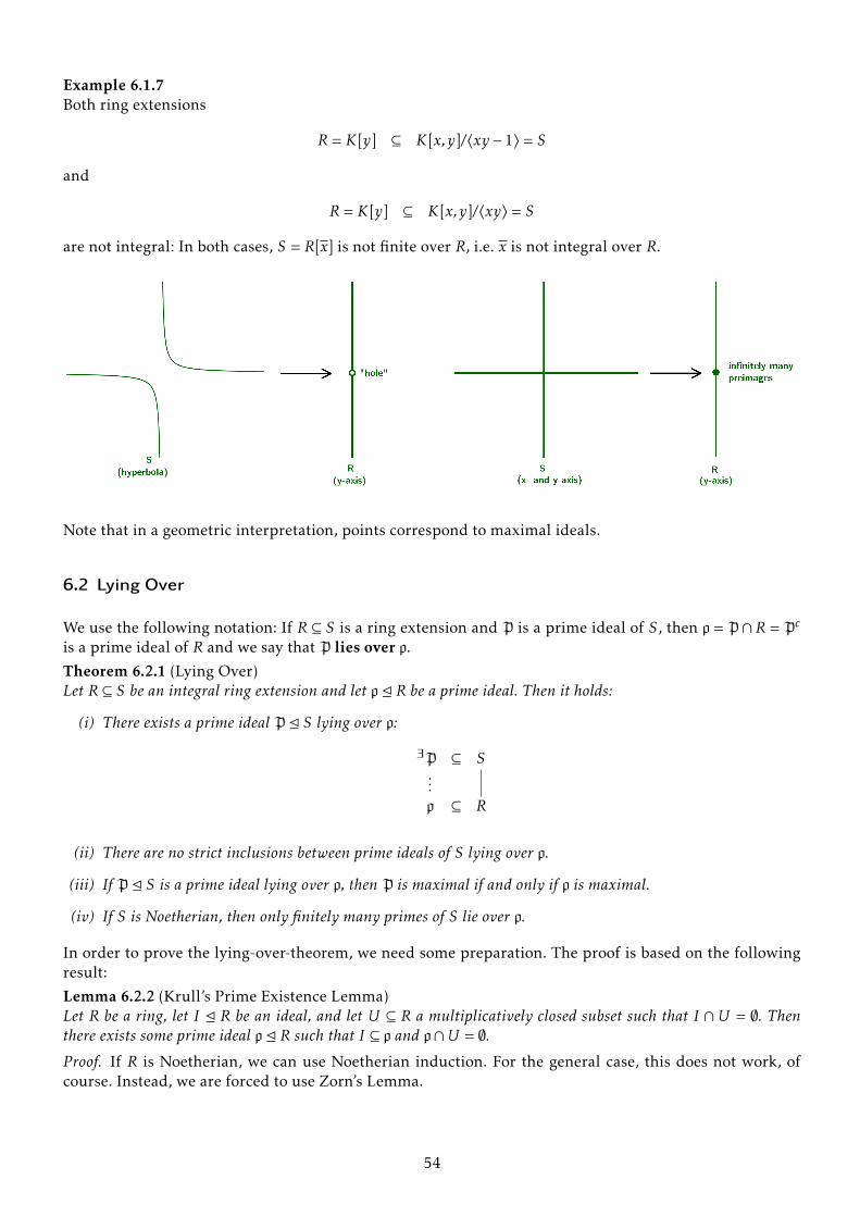
Example 6.1.7Both ring extensions

R = K[y] ⊆ K[x,y]/〈xy − 1〉 = S

and

R = K[y] ⊆ K[x,y]/〈xy〉 = S

are not integral: In both cases, S = R[x] is not finite over R, i.e. x is not integral over R.

Note that in a geometric interpretation, points correspond to maximal ideals.

6.2 Lying Over

We use the following notation: If R ⊆ S is a ring extension and P is a prime ideal of S, then p = P∩R = Pc

is a prime ideal of R and we say that P lies over p.

Theorem 6.2.1 (Lying Over)Let R ⊆ S be an integral ring extension and let p E R be a prime ideal. Then it holds:

(i) There exists a prime ideal P E S lying over p:

∃P ⊆ S...p ⊆ R

(ii) There are no strict inclusions between prime ideals of S lying over p.

(iii) If P E S is a prime ideal lying over p, then P is maximal if and only if p is maximal.

(iv) If S is Noetherian, then only finitely many primes of S lie over p.

In order to prove the lying-over-theorem, we need some preparation. The proof is based on the followingresult:

Lemma 6.2.2 (Krull’s Prime Existence Lemma)Let R be a ring, let I E R be an ideal, and let U ⊆ R a multiplicatively closed subset such that I ∩U = ∅. Thenthere exists some prime ideal p E R such that I ⊆ p and p∩U = ∅.Proof. If R is Noetherian, we can use Noetherian induction. For the general case, this does not work, ofcourse. Instead, we are forced to use Zorn’s Lemma.

54

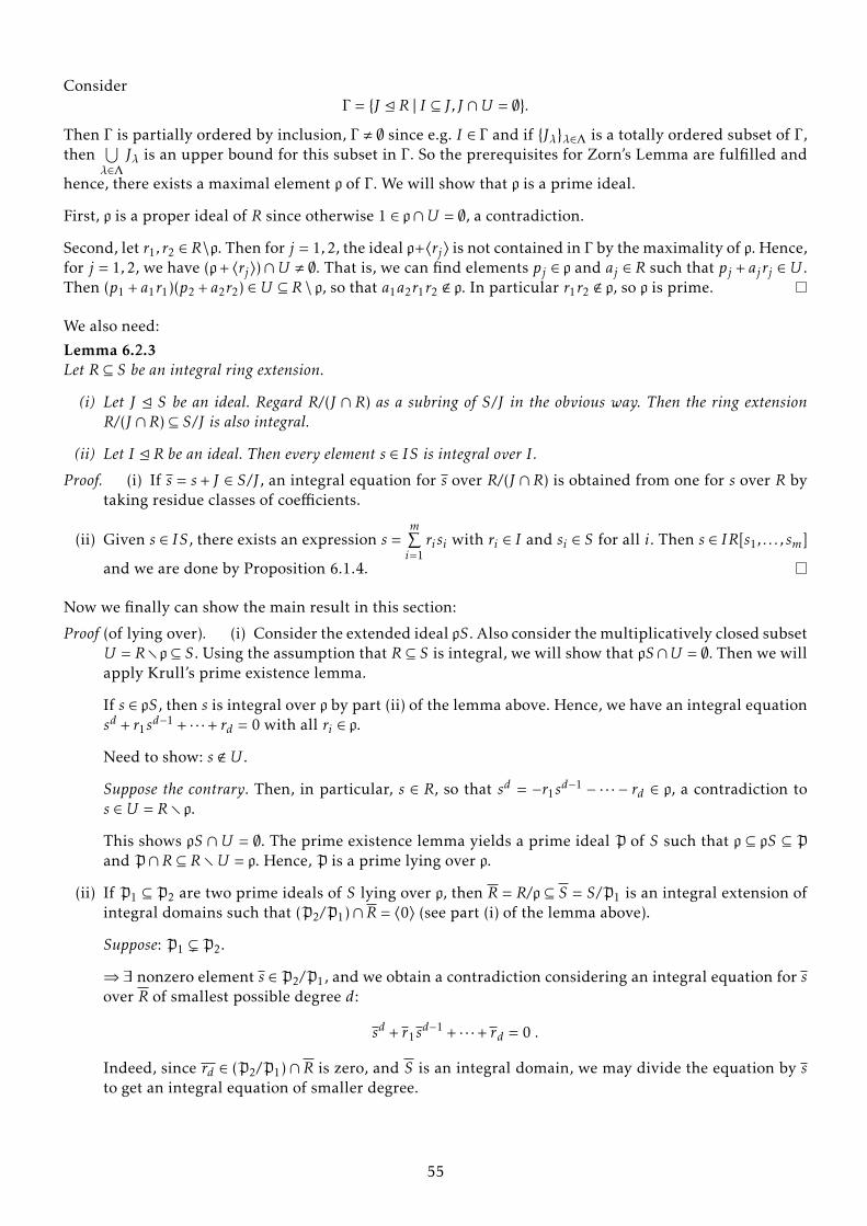
ConsiderΓ = {J E R | I ⊆ J, J ∩U = ∅}.

Then Γ is partially ordered by inclusion, Γ , ∅ since e.g. I ∈ Γ and if {Jλ}λ∈Λ is a totally ordered subset of Γ ,then

⋃λ∈Λ

Jλ is an upper bound for this subset in Γ . So the prerequisites for Zorn’s Lemma are fulfilled and

hence, there exists a maximal element p of Γ . We will show that p is a prime ideal.

First, p is a proper ideal of R since otherwise 1 ∈ p∩U = ∅, a contradiction.

Second, let r1, r2 ∈ R\p. Then for j = 1,2, the ideal p+〈rj〉 is not contained in Γ by the maximality of p. Hence,for j = 1,2, we have (p+ 〈rj〉)∩U , ∅. That is, we can find elements pj ∈ p and aj ∈ R such that pj + ajrj ∈U .Then (p1 + a1r1)(p2 + a2r2) ∈U ⊆ R \ p, so that a1a2r1r2 < p. In particular r1r2 < p, so p is prime.

We also need:

Lemma 6.2.3Let R ⊆ S be an integral ring extension.

(i) Let J E S be an ideal. Regard R/(J ∩ R) as a subring of S/J in the obvious way. Then the ring extensionR/(J ∩R) ⊆ S/J is also integral.

(ii) Let I E R be an ideal. Then every element s ∈ IS is integral over I .

Proof. (i) If s = s + J ∈ S/J , an integral equation for s over R/(J ∩R) is obtained from one for s over R bytaking residue classes of coefficients.

(ii) Given s ∈ IS, there exists an expression s =m∑i=1risi with ri ∈ I and si ∈ S for all i. Then s ∈ IR[s1, . . . , sm]

and we are done by Proposition 6.1.4.

Now we finally can show the main result in this section:

Proof (of lying over). (i) Consider the extended ideal pS. Also consider the multiplicatively closed subsetU = Rrp ⊆ S. Using the assumption that R ⊆ S is integral, we will show that pS∩U = ∅. Then we willapply Krull’s prime existence lemma.

If s ∈ pS, then s is integral over p by part (ii) of the lemma above. Hence, we have an integral equationsd + r1sd−1 + · · ·+ rd = 0 with all ri ∈ p.

Need to show: s <U .

Suppose the contrary. Then, in particular, s ∈ R, so that sd = −r1sd−1 − · · · − rd ∈ p, a contradiction tos ∈U = Rr p.

This shows pS ∩U = ∅. The prime existence lemma yields a prime ideal P of S such that p ⊆ pS ⊆ Pand P∩R ⊆ RrU = p. Hence, P is a prime lying over p.

(ii) If P1 ⊆ P2 are two prime ideals of S lying over p, then R = R/p ⊆ S = S/P1 is an integral extension ofintegral domains such that (P2/P1)∩R = 〈0〉 (see part (i) of the lemma above).

Suppose: P1 ( P2.

⇒∃ nonzero element s ∈ P2/P1, and we obtain a contradiction considering an integral equation for sover R of smallest possible degree d:

sd + r1sd−1 + · · ·+ rd = 0 .

Indeed, since rd ∈ (P2/P1)∩R is zero, and S is an integral domain, we may divide the equation by sto get an integral equation of smaller degree.

55

(iii) If p is maximal, then also P is maximal by (ii). For the converse, we consider the integral extensionR/p ⊆ S/P. If S/P is a field, its only maximal ideal is 〈0〉. Then, in turn, 〈0〉 is the only maximal idealof R/p by part (i), so that R/p is a field, too.

(iv) If P ⊆ S is a prime lying over p, then pS ⊆ P. By part (ii), P is a minimal prime of pS. Since S isNoetherian by assumption, Proposition 5.2.4 says that P is a minimal associated prime of pS, andthere exist only finitely many such primes.

Example 6.2.4The ring extension

R = Z ⊆ S = Z[√−5] � Z[x]/〈x2 + 5〉

is integral and the ideal p = 〈2〉 EZ is maximal. The ideal generated by 2 in Z[√−5], however, is not even a

prime ideal: (1 +√−5)︸ ︷︷ ︸

<〈2〉

· (1−√−5)︸ ︷︷ ︸

<〈2〉

= 6 = 3 · 2 ∈ 〈2〉. Using that

Z[√−5]/〈2〉 � F2[x]/〈x2 + 1〉 = F2[x]/〈(x+ 1)2〉,

we see that P = 〈2,1 +√−5〉 EZ[

√−5] is the only maximal ideal lying over 〈2〉 EZ.

A central property of integral ring extensions R ⊆ S is that nested pairs of prime ideals of R correspond tosuch pairs in S (naturally, this is important in the context of Krull dimension). Here is a first result in thisdirection:

Corollary 6.2.5 (Going-Up-Theorem of Cohen and Seidenberg)Let R ⊆ S be an integral ring extension. If p1 ⊆ p2 E R are prime ideals and P1 E S is a prime ideal lying over p1,then there exists a prime ideal P2 E S lying over p2 such that P1 ⊆ P2.

P1 ⊆ ∃P2...

p1 ⊆ p2

Proof. Applying the lying-over-theorem to the integral extension R = R/p1 ⊆ S = S/P1, we get a prime idealP2 E S lying over p2/p1. The preimage P2 of P2 in S has the desired properties.

6.3 Going Down

Once we had „Lying over“, „Going up“ was a relatively easy result. As we will show by example, for „Goingdown“ to hold , extra assumptions are needed.

Definition 6.3.1Let R be an integral domain. The integral closure of R in its quotient field Q(R),

R = {s ∈Q(R) | s integral over R}

is called the normalization of R. We call R normal if R = R.

Finding algorithms for computing the normalization of a ring of type K[x1, . . . ,xn]/I is an active area ofresearch in Computer Algebra.

Example 6.3.2 (i) If R is a unique factorization domain, then R is normal.

(ii) In particular, K[x1, . . . ,xn] is normal.

56

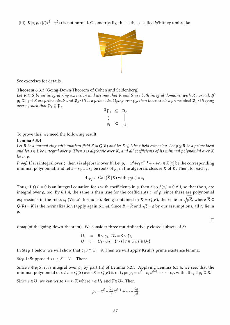
(iii) K[x,y,z]/〈x2 − y2z〉 is not normal. Geometrically, this is the so called Whitney umbrella:

See exercises for details.

Theorem 6.3.3 (Going-Down-Theorem of Cohen and Seidenberg)Let R ⊆ S be an integral ring extension and assume that R and S are both integral domains, with R normal. Ifp1 ⊆ p2 E R are prime ideals and P2 E S is a prime ideal lying over p2, then there exists a prime ideal P1 E S lyingover p1 such that P1 ⊆ P2.

∃P1 ⊆ P2...p1 ⊆ p2

To prove this, we need the following result:

Lemma 6.3.4Let R be a normal ring with quotient field K =Q(R) and let K ⊆ L be a field extension. Let p E R be a prime idealand let s ∈ L be integral over p. Then s is algebraic over K , and all coefficients of its minimal polynomial over Klie in p.

Proof. If s is integral over p, then s is algebraic overK . Let ps = xd+c1xd−1+· · ·+cd ∈ K[x] be the corresponding

minimal polynomial, and let s = s1, . . . , sd be roots of ps in the algebraic closure K of K . Then, for each j,

∃ ϕj ∈ Gal (K |K) with ϕj(s) = sj .

Thus, if f (s) = 0 is an integral equation for s with coefficients in p, then also f (sj ) = 0 ∀ j, so that the sj areintegral over p, too. By 6.1.4, the same is then true for the coefficients ci of ps since these are polynomial

expressions in the roots sj (Vieta’s formulas). Being contained in K = Q(R), the ci lie in√pR, where R ⊆

Q(R) = K is the normalization (apply again 6.1.4). Since R = R and√p = p by our assumptions, all ci lie in

p.

Proof (of the going-down-theorem). We consider three multiplicatively closed subsets of S:

U1 = Rr p1, U2 = S rP2U := U1 ·U2 = {r · s | r ∈U1, s ∈U2}

In Step 1 below, we will show that p1S ∩U = ∅. Then we will apply Krull’s prime existence lemma.

Step 1: Suppose ∃ s ∈ p1S ∩U . Then:

Since s ∈ p1S, it is integral over p1 by part (ii) of Lemma 6.2.3. Applying Lemma 6.3.4, we see, that theminimal polynomial of s ∈ L =Q(S) over K =Q(R) is of type ps = xd + c1x

d−1 + · · ·+ cd , with all ci ∈ p1 ⊆ R.

Since s ∈U , we can write s = r · s, where r ∈U1 and s ∈U2. Then

ps = xd +c1

rxd−1 + · · ·+ cd

rd

57

is the minimal polynomial of s over K . Applying again Lemma 6.3.4, we see that the coefficients ci/r i of pslie in R, since s is integral over R by assumption. In fact, the ci/r i lie in p1 since ci ∈ p1 and r i < p1 ∀ i. Itfollows that s is even integral over p1. So s ∈

√p1S ⊆ P2 by Proposition 6.1.4, a contradiction to s ∈U2.

Step 2: Krull’s prime existence lemma yields a prime ideal P1 ⊆ S such that p1S ⊆ P1 and P1 ∩U = ∅. Inparticular, P1∩U1 = ∅, so that P1∩R = p1, that is, P1 is lying over p1, and P1∩U2 = ∅, so that P1 ⊆ P2.

To indicate that the additional assumptions in the going-down-theorem are needed, we will give an exam-ple. To prepare for this, we state a couple of remarks.

Remark 6.3.5Let K be a field. If p = (a1, . . . , an) ∈ Kn is a point, each polynomial f ∈ K[x1, . . . ,xn] can be written as apolynomial in the xi − ai :

f = f (p) + terms of degree at least 1 in the xi − ai (∗)

Indeed, to obtain this Taylor expression of f at p, substitute the (xi − ai) + ai for the xi in f and expand.

It follows from (∗) that mp = 〈x1 − a1, . . . ,xn − an〉 is the kernel of the evaluation map K[x1, . . . ,xn] → K ,f 7→ f (p). Hence, K[x1, . . . ,xn]/mp � K is a field, so mp is a maximal ideal.

Note that in general, not every maximal ideal of K[x1, . . . ,xn] is of the above type. Consider, for instance,〈1 + x2〉 ER[x]. We will come back to this later in the context of Hilbert’s Nullstellensatz.

Remark 6.3.6 (i) Examples 6.1.7, 6.3.2, (iii) involved rings which are finitely generated K-algebras (whe-re K is a field), i.e. quotient rings of type K[x1, . . . ,xn]/I (where I is an ideal). We call any such ring anaffine ring, and if I is a prime ideal, we call the ring an affine domain.

(ii) Every extension R ⊆ S of affine rings is obviously of finite type. Hence, in this case, R ⊆ S is integralif and only if R ⊆ S is finite. Using computer algebra, this condition can be checked via Gröbnerbases. These “bases” are special generators for ideals in polynomial rings over a field which can becomputed using an algorithm by Buchberger. The definition of Gröbner bases and their computa-tion depends on monomial orderings which allow us to distinguish a leading monomial for everypolynomial. In our context, consider a ring homomorphism of type

ϕ : K[y1, . . . , ym]→ K[x1, . . . ,xn]/I .

To give such a homomorphism, it is equivalent to give the images fj = fj + I of the variables yj . Nowconsider the ideal

J = 〈I, f1 − y1, . . . , fm − ym〉 E K[x1, . . . ,xn, y1, . . . , ym],

and let g1, . . . , gr be a Gröbner basis for J with respect to the lexicographic monomial ordering onK[x1, . . . ,xn, y1, . . . , ym]. Then, as one can show, the following two statements hold:

a) The gk not depending on any of the xi generate kerϕ.

b) The ring extensionϕ : K[y1, . . . , ym]/ kerϕ→ K[x1, . . . ,xn]/I

is finite if and only if for each i there exists a gk whose leading monomial is of type xαii for someαi ≥ 1.

Example 6.3.7Consider the homomorphism ϕ : K[x,y,z]→ K[s, t] with x 7→ s, y 7→ t2 − 1 and z 7→ t(t2 − 1). We use theabove remark to study ϕ:

Computing the (reduced) lexicographic Gröbner basis for the ideal

J = 〈s − x, t2 − 1− y, t(t2 − 1)− z〉 E K[s, t,x,y,z],

58

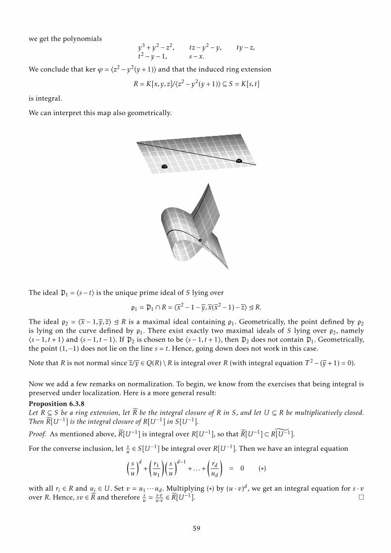
we get the polynomialsy3 + y2 − z2, tz − y2 − y, ty − z,t2 − y − 1, s − x.

We conclude that ker ϕ = 〈z2 − y2(y + 1)〉 and that the induced ring extension

R = K[x,y,z]/〈z2 − y2(y + 1)〉 ⊆ S = K[s, t]

is integral.

We can interpret this map also geometrically.

The ideal P1 = 〈s − t〉 is the unique prime ideal of S lying over

p1 = P1 ∩R = 〈x2 − 1− y,x(x2 − 1)− z〉 E R.

The ideal p2 = 〈x − 1, y,z〉 E R is a maximal ideal containing p1. Geometrically, the point defined by p2is lying on the curve defined by p1. There exist exactly two maximal ideals of S lying over p2, namely〈s − 1, t + 1〉 and 〈s − 1, t − 1〉. If P2 is chosen to be 〈s − 1, t + 1〉, then P2 does not contain P1. Geometrically,the point (1,−1) does not lie on the line s = t. Hence, going down does not work in this case.

Note that R is not normal since z/y ∈Q(R) \R is integral over R (with integral equation T 2 − (y + 1) = 0).

Now we add a few remarks on normalization. To begin, we know from the exercises that being integral ispreserved under localization. Here is a more general result:

Proposition 6.3.8Let R ⊆ S be a ring extension, let R be the integral closure of R in S, and let U ⊆ R be multiplicatively closed.Then R[U−1] is the integral closure of R[U−1] in S[U−1].

Proof. As mentioned above, R[U−1] is integral over R[U−1], so that R[U−1] ⊂ ˜R[U−1].

For the converse inclusion, let su ∈ S[U−1] be integral over R[U−1]. Then we have an integral equation( su

)d+(r1u1

)( su

)d−1+ . . .+

(rdud

)= 0 (∗)

with all ri ∈ R and ui ∈ U . Set v = u1 · · ·ud . Multiplying (∗) by (u · v)d , we get an integral equation for s · vover R. Hence, sv ∈ R and therefore s

u = s·vu·v ∈ R[U−1].

59

Next we show that being normal is a local property.

Proposition 6.3.9Let R be an integral domain. Then the following are equivalent:

(i) R is normal.

(ii) Rp is normal for all prime ideals p E R.

(iii) Rm is normal for all maximal ideals m E R.

Proof. Let R ⊆ Q(R) be the normalization of R. Consider the inclusion i : R ↪→ R. Then R is normal if andonly if i is surjective. Furthermore, by 6.3.8, Rp (resp. Rm) is normal if and only if ip (resp. im) is surjective.The result follows since being surjective is a local property (see 3.2.2).

Finally, we note:

Remark 6.3.10If R is a Noetherian integral domain, then R need not be Noetherian as well (see Nagata’s textbook). If Ris an affine domain, however, then R is finite over R, and R is again an affine domain. This is an importantfiniteness result by Emmy Noether.

60

7 Krull Dimension, Noether Normalization, Hilbert’s Nullstellensatz and

Krull’s Principle Ideal Theorem

7.1 Definition of Krull Dimension

We recall the definition of Krull dimension. Let R be a ring. A sequence p0 ( p1 ( . . . ( pm of prime idealsof R with strict inclusions is called a chain of prime ideals of R of length m. We call the chain maximal ifit cannot be extended to a larger chain by inserting an extra prime ideal.

Definition 7.1.1Let R be a ring. The Krull dimension of R, written dimR, is the supremum of the lengths of chains ofprime ideals of R. If I E R is a proper ideal, the dimension of I , written dim I , is defined to be dimR/I .

Example 7.1.2Each non-zero prime ideal of Z is of type 〈p〉, where p is a prime number. Hence,

dimZ = 1.

More generally, each principle ideal domain which is not a field has Krull dimension 1.

Note that even Noetherian rings may have infinite dimension (see the appendix of Nagata’s textbook)!

Proposition 7.1.3If R ⊆ S is an integral ring extension, then R and S have the same dimension: dimR = dimS.

Proof. By „Lying over“ and „Going up“, each chain of prime ideals of R gives rise to one of S.

Conversely, if P0 ( P1 ( . . . ( Pm is a chain of prime ideals of S, the contractions Pi ∩R form such a chainin R (all inclusions are strict by part (ii) of lying over).

Remark 7.1.4Consider the polynomial ring K[x1, . . . ,xn]. Intuitively, we would expect that dimK[x1, . . . ,xn] = n. In fact,we can easily see that dimK[x1, . . . ,xn] ≥ n since

〈0〉 ( 〈x1〉 ( 〈x1,x2〉 ( . . . ( 〈x1, . . . ,xn〉

is a chain of prime ideals in K[x1, . . . ,xn].

To show that the dimension of K[x1, . . . ,xn] is exactly n, we use the concept of Noether normalization.

7.2 Noether Normalization

We start with two Lemmata.

Lemma 7.2.1Let K be an infinite field and let f ∈ K[x1, . . . ,xn] be a non-zero polynomial. Then there exists a point p =(a1, . . . , an) ∈ Kn such that f (p) , 0.

Proof. We use induction on n.

For n = 1, the statement is clear, since each non-zero polynomial in one variable has at most finitely manyzeros.

If n > 1, we write f in the form f = c0(x2, . . . ,xn)xe1 + . . .+ ce(x2, . . . ,xn). Then ci , 0 for at least one i. For suchan i, by induction, there exists a point p′ ∈ Kn−1 such that ci(p′) , 0. Then 0 , f (x1,p

′) ∈ K[x1], hence thereexists an element of a ∈ K such that f (a,p′) , 0.

61

In the proof of the second lemma, we use the following notation.

Remark 7.2.2Let R be a ring. A polynomial in R[x1, . . . ,xn] is called homogeneous (of degree e) if all its monomials havedegree e or if the polynomial is zero.

Every nonzero polynomial f ∈ R[x1, . . . ,xn] of degree e can be uniquely written as a sum f = fe + fe−1 +· · · + f0, where the fi are homogenenous of degree i, and where fe , 0. The fi are called the homogeneouscomponents of f .

Given an extra variable x0, the polynomial

f h := xe0f (x1/x0, . . . ,xn/x0) ∈ R[x0,x1, . . . ,xn]

is homogeneous of degree e, and is called the homogenization of f with respect to x0.

Conversely, the dehomogenization of a homogeneous polynomial F ∈ R[x0,x1, . . . ,xn] with respect to x0 isdefined to be the polynomial F(1,x1, . . . ,xn) ∈ R[x1, . . . ,xn]. We have

f h(1,x1, . . . ,xn) = f and F = xm0 ·F(1,x1, . . . ,xn)h,

where m is the highest power of x0 dividing F.

Lemma 7.2.3Let K be a field and let f ∈ K[x1, . . . ,xn] \K be a non-constant polynomial.

(i) Let K be infinite. If a2, . . . , an ∈ K are sufficiently general, then the isomorphism

K[x1,x2, . . . ,xn] → K[x1, x2, . . . , xn]

x1 7→ x1, xi 7→ xi + aix1 for i = 2, . . . ,n

maps f to a polynomial of type axe1 + c1(x2, . . . , xn)xe−11 + . . .+ ce(x2, . . . , xn), where a ∈ K is non-zero, e ≥ 1,

and each ci ∈ K[x2, . . . , xn].

(ii) If K is arbitrary, the same is achieved by sending

K[x1,x2, . . . ,xn] → K[x1, x2, . . . , xn]

x1 7→ x1, xi 7→ xi + xri−1

1 for i = 2, . . . ,n,

where r is sufficiently large.

Proof. (i) Let f = fe + fe−1 + . . .+ f0, fe , 0, be the decomposition of f into its homogeneous componentsfi of degree i. After substituting xi + aix1 for xi in f , i = 2, . . . ,n, the coefficient of xe1 is fe(1, a2, . . . , an).Now, by writing

fe = xm1 fe(1,x2, . . . ,xn)h

as in the remark above, we see that fe(1,x2, . . . ,xn) , 0 since fe , 0. Since K is infinite, by the previouslemma, there exist a2, . . . , an ∈ K , such that fe(1, a2, . . . , an) , 0. The result follows.

(ii) Write f as the finite sum of its terms,

f =∑

xα1...αnxα11 · · ·x

αnn ,

and let r ∈N. After substituting xi + xri−1

1 in f for xi , i = 2, . . . ,n, the terms depending only on x1 are

of type cα1...αnxα1+α2r+...+αnrn−1

1 . If r is strictly larger than all αi appearing in a term of f , the numbersα1 +α2r + . . .+αnrn−1 are distinct for distinct α1, . . . ,αn (the αi are the digits in the base–r expansionof the exponent). Hence, the terms depending only on x1 cannot cancel with each other. The resultfollows.

62

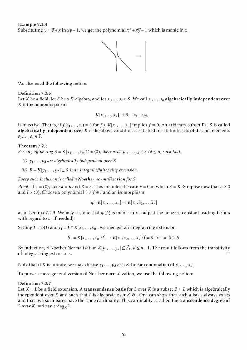
Example 7.2.4Substituting y = y + x in xy − 1, we get the polynomial x2 + xy − 1 which is monic in x.

We also need the following notion.

Definition 7.2.5Let K be a field, let S be a K-algebra, and let s1, . . . , sn ∈ S. We call s1, . . . , sn algebraically independent overK if the homomorphism

K[x1, . . . ,xn]→ S, xi 7→ si ,

is injective. That is, if f (s1, . . . , sn) = 0 for f ∈ K[x1, . . . ,xn] implies f = 0. An arbitrary subset Γ ⊂ S is calledalgebraically independent over K if the above condition is satisfied for all finite sets of distinct elementss1, . . . , sn ∈ Γ .

Theorem 7.2.6For any affine ring S = K[x1, . . . ,xn]/I , 〈0〉, there exist y1, . . . , yd ∈ S (d ≤ n) such that:

(i) y1, . . . , yd are algebraically independent over K .

(ii) R = K[y1, . . . , yd] ⊆ S is an integral (finite) ring extension.

Every such inclusion is called a Noether normalization for S.

Proof. If I = 〈0〉, take d = n and R = S. This includes the case n = 0 in which S = K . Suppose now that n > 0and I , 〈0〉. Choose a polynomial 0 , f ∈ I and an isomorphism

ϕ : K[x1, . . . ,xn]→ K[x1, x2, . . . , xn]

as in Lemma 7.2.3. We may assume that ϕ(f ) is monic in x1 (adjust the nonzero constant leading term awith regard to x1 if needed).

Setting I = ϕ(I) and I1 = I ∩K[x2, . . . , xn], we then get an integral ring extension

S1 = K[x2, . . . , xn]/ I1→ K[x1, x2, . . . , xa]/ I = S1[x1] =: S � S.

By induction, ∃ Noether Normalization K[y1, . . . , yd] ⊆ S1, d ≤ n−1. The result follows from the transitivityof integral ring extensions.

Note that if K is infinite, we may choose y1, . . . , yd as a K-linear combination of x1, . . . ,xn.

To prove a more general version of Noether normalization, we use the following notion:

Definition 7.2.7Let K ⊆ L be a field extension. A transcendence basis for L over K is a subset B ⊆ L which is algebraicallyindependent over K and such that L is algebraic over K(B). One can show that such a basis always existsand that two such bases have the same cardinality. This cardinality is called the transcendence degree ofL over K , written trdegKL.

63

For example, ifK(x1, . . . ,xn) =Q(K[x1, . . . ,xn]

is the field of rational functions in the variables x1, . . . ,xn, then

trdegKK(x1, . . . ,xn) = n.

Theorem 7.2.8 (Noether Normalization, Refined Version)Let S = K[x1, . . . ,xn]/I , 〈0〉 be an affine ring, and let J E S ba a proper ideal. Then there exist numbers δ ≤ d ≤ nand a Noether normalization K[y1, . . . , yd] ⊆ S such that

J ∩K[y1, . . . , yd] = 〈y1, . . . , yδ〉.

Proof. Let K[z1, . . . , zd] ⊆ S be any Noether normalization. By the transitivity of integral extensions, it isenough to find a Noether normalization K[y1, . . . , yd] ⊆ K[z1, . . . , zd] such that J ∩K[y1, . . . , yd] = 〈y1, . . . , yδ〉for some δ ≤ d. We may, thus, suppose that S = K[z1, . . . , zd] is a polynomial ring.

In this case, if J = 〈0〉, there is nothing to show.

Otherwise, if J , 〈0〉, by 7.2.3, we may suppose that the coordinates are chosen such that J contains a monicpolynomial

f = ze1 + c1ze−1 + . . .+ ce with all ci ∈ K[z2, . . . , zd].

Let y1 := f . Then K[y1, z2, . . . , zd] ⊆ K[z1, . . . , zd] = K[y,z2, . . . , zd][z1] is an integral ring extension.

On the other hand, by induction, there exists a Noether normalization K[y2, . . . , yd] ⊂ K[z2, . . . , zd] such thatJ ∩K[y2, . . . , yd] = 〈y2, . . . , yδ〉 for some δ ≤ d.

Then K[y1, y2, . . . , yd] ⊆ K[y1, z2, . . . , zd] ⊆ K[z1, . . . , zd] is integral as well. Moreover, y1, . . . , yd are algebraical-ly independent over K since, otherwise, trdegK (K(z1, . . . , zd)) would be smaller than d, contradicting thealgebraic independence of the zi over K .

Finally, since each g ∈ J ∩ K[y1, . . . , yd] can be written as a sum g = g1y1 + h, with g1 ∈ K[y1, . . . , yd] andh ∈ J ∩K[y2, . . . , yd] = 〈y2, . . . , yδ〉, we conclude that J ∩K[y1, . . . , yd] = 〈y1, . . . , yδ〉.

7.3 Properties of Krull Dimension

Theorem 7.3.1Let K be a field. Then the polynomial ring K[x1, . . . ,xn] has Krull dimension n. In fact, every maximal chain ofprime ideals of K[x1, . . . ,xn] has length n.

Proof. For both statements, we do induction on n. The case n = 0 is clear.

Now suppose that n ≥ 1, and letP0 ( P1 ( . . . ( Pm (∗)

be a chain of of prime ideals of K[x1, . . . ,xn]. By extending the chain, we may assume that P0 = 〈0〉 sincethis is the smallest prime ideal in the integral domain K[x1, . . . ,xn]. Moreover, we may assume that Pm is amaximal ideal. In particular, m ≥ 1.

We proceed in three steps.

Step 1. We show that m ≤ n. Applying Theorem 7.2.8 and the transcendence degree argument fromits proof to P1, we get a Noether normalization K[y1, . . . , yn] ⊂ K[x1, . . . ,xn] such that P1 ∩ K[y1, . . . , yn] =〈y1, . . . , yδ〉 for some δ ≤ n. For all i, set pi = Pi ∩K[y1, . . . , yn]. Then

p1/p1 ( p2/p1 ( . . . ( pm/p1

64

is a chain of prime ideals in the ring K[y1, . . . , yn]/p1 � K[yδ+1, . . . , yn]. By the induction hypothesis, m − 1 ≤n − δ. So m ≤ n since δ ≥ 1 (otherwise, both P0 and P1 would lie over the zero ideal of K[y1, . . . , yn], acontradiction to part 2 of the lying over theorem). This shows the first part of the theorem.

Step 2. Now assume that (∗) is a maximal chain of prime ideals. Then the induced chain

〈0〉 = p0 ( p1 ( · · · ( pm (∗∗)

of prime ideals of K[y1, . . . , yn] is maximal as well: Suppose, to the contrary, that there is a prime idealq ⊂ K[y1, . . . , yn] with strict inclusions pi ( q ( pi+1 for some i. Then 0 ≤ i ≤m−1 since pm is maximal by part3 of the lying over theorem. Applying Theorem 7.2.8 to pi , we get a Noether normalization K[z1, . . . , zn] ⊂K[y1, . . . , yn] such that pi ∩K[z1, . . . , zn] = 〈z1, . . . , zδ′〉 for some δ′ ≤ n. Then the composition

K[zδ′+1, . . . , zn] ⊂ K[y1, . . . , yn]→ K[y1, . . . , yn]/pi

is a Noether normalization as well, and we have strict inclusions

〈0〉 ( (q/pi)∩K[zδ′+1, . . . , zn] ( (pi+1/pi)∩K[zδ′+1, . . . , zn].

Since K[zδ′+1, . . . , zn] ⊂ K[x1, . . . ,xn]/Pi is also a Noether normalization by 6.2.3, we see by going down thatwe may insert a prime ideal between 〈0〉 and Pi+1/Pi in K[x1, . . . ,xn]/Pi and, thus, also between Pi and Pi+1in K[x1, . . . ,xn]. This contradicts the maximality of (∗). We conclude that (∗∗) is maximal, too. In particular,we see that δ = 1 in Step 1.

Step 3. The maximal chain (∗∗) corresponds to a maximal chain of prime ideals of

K[y1, . . . , yn]/p1 = K[y1, . . . , yn]/〈y1〉 � K[y2, . . . , yn]

of length m− 1. So m− 1 = n− 1 by the induction hypothesis, and we are done.

Corollary 7.3.2Let R be an affine domain over a field K . Then

dimR = trdegKQ(R).

This is the common length of all maximal chains of prime ideals of R.

Proof. Let K[y1, . . . , yd] ⊆ R be a Noether Normalization. Then dimR7.1.3= dimK[y1, . . . , yd] 7.3.1= d. Since also

trdegKQ(R) = trdegK(y1 . . . , yd) = d, we have dimR = trdegKQ(R).

For the second statement, write R as a quotient K[x1, . . . ,xn]/q, where q is a prime ideal, and fix a chainq0 = 〈0〉 ( . . . ,( qc = q of prime ideals of K[x1, . . . ,xn] which cannot be extended to a longer such chain withlargest ideal q. The fixed chain and the preimage of any maximal chain of prime ideals of R fit together togive a maximal chain of prime ideals of the polynomial ring K[x1, . . . ,xn]. This, however, has length n byTheorem 7.3.1. The result follows.

The following notion gives one way of measuring the size of an ideal.

Definition 7.3.3Let R be a ring and let I E R be a proper ideal. The codimension of I , written codim I , is defined as follows:If I = P is a prime ideal, take the supremum of the lengths of all chains of prime ideals of R with largestprime P . If I is arbitrary, take the minimum of the length of prime ideals containing I .

Corollary 7.3.4Let R be an affine domain over a field K and let I E R a proper ideal. Then

dim I + codim I = dimR.

65

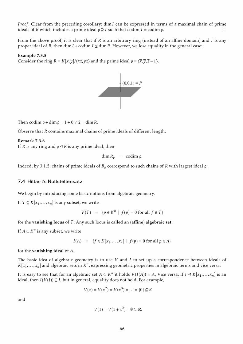
Proof. Clear from the preceding corollary: dim I can be expressed in terms of a maximal chain of primeideals of R which includes a prime ideal p ⊇ I such that codim I = codim p.

From the above proof, it is clear that if R is an arbitrary ring (instead of an affine domain) and I is anyproper ideal of R, then dim I + codim I ≤ dimR. However, we lose equality in the general case:

Example 7.3.5Consider the ring R = K[x,y]/〈xz,yz〉 and the prime ideal p = 〈x,y,z − 1〉.

(0,0,1) = P

Then codim p+ dimp = 1 + 0 , 2 = dimR.

Observe that R contains maximal chains of prime ideals of different length.

Remark 7.3.6If R is any ring and p E R is any prime ideal, then

dimRp = codim p.

Indeed, by 3.1.5, chains of prime ideals of Rp correspond to such chains of R with largest ideal p.

7.4 Hilbert’s Nullstellensatz

We begin by introducing some basic notions from algebraic geometry.

If T ⊆ K[x1, . . . ,xn] is any subset, we write

V (T ) = {p ∈ Kn | f (p) = 0 for all f ∈ T }

for the vanishing locus of T . Any such locus is called an (affine) algebraic set.

If A ⊆ Kn is any subset, we write

I(A) = {f ∈ K[x1, . . . ,xn] | f (p) = 0 for all p ∈ A}

for the vanishing ideal of A.

The basic idea of algebraic geometry is to use V and I to set up a correspondence between ideals ofK[x1, . . . ,xn] and algebraic sets in Kn, expressing geometric properties in algebraic terms and vice versa.

It is easy to see that for an algebraic set A ⊆ Kn it holds V (I(A)) = A. Vice versa, if J E K[x1, . . . ,xn] is anideal, then I(V (J)) ⊆ J , but in general, equality does not hold. For example,

V (x) = V (x2) = V (x3) = . . . = {0} ⊆ K

and

V (1) = V (1 + x2) = ∅ ⊆R.

66

To get rid of problems of the first type, we may restrict ourselves to radical ideals. With respect to thesecond problem, algebraic geometers prefer to work over an algebraically closed field.

Hilbert’s Nullstellensatz tells us, that over such a field, V and I define a one-to-one-correspondence bet-ween algebraic subsets of Kn and radical ideals of K[x1, . . . ,xn]. Under this correspondence, irreduciblealgebraic sets correspond to prime ideals, and points to maximal ideals.

We discuss one way of deducing the Nullstellensatz from Noether normalization (there are also severalother possible approaches).

Theorem 7.4.1Let K be an algebraically closed field. Then the maximal ideals of K[x1, . . . ,xn] are precisely the ideals of typemp = 〈x1 − a1, . . . ,xn − an〉, where p = (a1, . . . , an) ∈ Kn.

Proof. We already know from 6.3.5 that each ideal of type mp is a maximal ideal of K[x1, . . . ,xn].

Conversely, let m E K[x1, . . . ,xn] be any maximal ideal. Then L = K[x1, . . . ,xn]/m is a field. Hence, if R =K[y1, . . . , yd] ⊆ L is a Noether normalization, we must have R = K since otherwise

0 = dimL = dimK[y1, . . . , yd] = d ≥ 1.

Then K ⊆ L is a finite, hence algebraic field extension. Since K is algebraically closed, the inclusion K ⊆ Lis an isomorphism. Hence, there exist a1, . . . , an ∈ K such that ai can be identified with the residue class xi ,i.e. ai = xi for all i = 1, . . . ,n. Thus, 〈x1 − a1, . . . ,xn − an〉 ⊆m. Since 〈x1 − a1, . . . ,xn − an〉 is a maximal ideal andm is a proper ideal, these ideals must coincide.

Note that this theorem says nothing else than the concise statement from above: „points p correspond tomaximal ideals mp“.

Theorem 7.4.2 (Hilbert’s Nullstellensatz, weak version)Let K be an algebraically closed field and let I E K[x1, . . . ,xn] be an ideal. Then the following are equivalent:

(i) V (I) ⊆ Kn is empty.

(ii) 1 ∈ I .Proof. ”(ii)⇒ (i)” is clear.

”(i)⇒ (ii)”: If 1 < I , then I is a proper ideal of K[x1, . . . ,xn]. Hence, I is contained in a maximal ideal, whichby 7.4.1 is of type mp = 〈x1 − a1, . . . ,xn − an〉 for some p = (a1, . . . , an) ∈ Kn. Since I ⊆m implies V (I) ⊇ V (m),we conclude that {p} = V (m) ⊆ V (I), hence V (I) , ∅.Theorem 7.4.3 (Hilbert’s Nullstellensatz, strong version)Let K be an algebraically closed field and let I E K[x1, . . . ,xn] be an ideal. Then

I(V (I)) =√I .

Proof. ”⊇”: If f ∈√I , then f m ∈ I for some m ≥ 1. This implies that f m and, thus, also f vanish on V (I). We

conclude that f ∈ I(V (I)).

”⊇”: Let now f ∈ I(V (I)), and let I = 〈f1, . . . , fr〉. Then f vanishes on V (I), and we have to show that f m =r∑i=1gifi for some m ≥ 1 and some g1, . . . , gr ∈ K[x1, . . . ,xn] =: R.

We use the trick of Rabinowitch: Consider the ideal

J := 〈f1, . . . , fr ,1− tf 〉 ⊆ R[t],

where t is an extra variable. We show that V (J) ⊆ Kn+1 is empty and apply the weak version of the Null-stellensatz.

67

Suppose the contrary: ∃ p = (a1, . . . , an, an+1) ∈ V (J).

Set p′ = (a1, . . . , an) ∈ Kn. Then f1(p′) = · · · = fr(p′) = 0, so that p′ ∈ V (I), and an+1f (p′) = 1. This contradictsthe fact that f vanishes on V (I).

Applying the weak version of the Nullstellensatz, we get 1 ∈ J . That is, 1 =r∑i=1hifi + h(1 − tf ) for suitable

h1, . . . ,hr ,h ∈ R(t]. Substituting 1/f for t in this expression (formally work in R(t]f ) and multiplying by a

sufficiently high power f m to clear denominators, we get a representation f m =r∑i=1gifi as desired.

7.5 Krull’s Principal Ideal Theorem and Regular Local Rings

Theorem 7.5.1 (Krull’s Principal Ideal Theorem, first version)Let R be a Noetherian ring and let f ∈ R. Then each minimal prime p of 〈f 〉 satisfies

codim p ≤ 1.

If f is not a zero-divisor of R, then equality holds.

Proof. The second statement follows from the first one: Since R is Noetherian, by 5.2.5, the nonzerodivisorf is not contained in any of the (finitely many) minimal primes of R. Hence, codim (p) ≥ 1.

To show the first statement, we localize and apply Nakayama’ lemma. To begin with, by Remark 7.3.6, wehave codim p = dimRp. Furthermore, by Theorem 3.1.5, the extended prime ideal pRp is a minimal primeof the extended ideal 〈f 〉Rp. Replacing R by Rp, we may, hence, assume that (R,p) is a local ring.

Then for any prime ideal q of R with q ( p, we must show

codim q = dimRq = 0.

Given such a q, we consider the ideals

q(n) := {a ∈ R | va ∈ qn for some v < q}, n ≥ 1.

Then, by Theorem 5.2.5, q(n) is the preimage (qn)ec of (qn)e = qnRq under R→ Rq. Since the maximal idealp/〈f 〉 of R/〈f 〉 is also a minimal prime of R/〈f 〉 by the assumption on p, the ring R/〈f 〉 is zero–dimensional.Being also Noetherian, it is Artinian by Theorem 4.4.2. Hence, the descending chain

q(1) + 〈f 〉 ⊇ q(2) + 〈f 〉 ⊇ . . .

is eventually stationary, sayq(n) + 〈f 〉 = q(n+1) + 〈f 〉.

We may then write any g ∈ q(n) as g = h+ af , with h ∈ q(n+1) and a ∈ R. Then af ∈ q(n). Since p is a minimalprime of 〈f 〉, we have f < q and, hence, a ∈ q(n) by the very definition of q(n). This shows:

q(n+1) + f q(n) = q(n).

Since 〈f 〉 ⊆ p and p is a maximal ideal by our assumption above, Nakayama’s lemma applied over R yieldsq(n) = q(n+1). Then qnRq = qn+1Rq by 3.1.5. Applying Nakayama’s lemma over Rq, we get qnRq = 〈0〉 (“themaximal ideal of qnRq is nilpotent”). We conclude from 1.8.1, 1.8.2 that dimRq = 0.

The general version of the Principal Ideal Theorem provides a lower bound for the number of equations ofan algebraic set of a given codimension.

68

Theorem 7.5.2 (Krull’s Principal Ideal Theorem, general version)Let R be a Noetherian ring and let I = 〈f1, . . . , fc〉 E R be an ideal generated by c elements. Then each minimalprime p of I satisfies

codim p ≤ c.

Conversely, if p E R is a prime ideal of codimension c, then there exist y1, . . . , yc ∈ R such that p is a minimal primeof 〈y1, . . . , yc〉.Proof. For the first statement, let p be a minimal prime of I . As in the preceding proof, we may assume that(R,p) is a local ring. We do induction on c.

The result is clear for c = 1 by 7.5.1.

Suppose now that c > 1 and that q ( p is a prime ideal of R with no other prime ideal of R between q and p(if no such q exists, then codim I = codim p = 0).

Since p is a minimal prime of I = 〈f1, . . . , fc〉, at least one of the fi is not contained in q, say fc < q. Then themaximal ideal p/(q + 〈fc〉) of R/(q + 〈fc〉) is also a minimal prime of this ring. Arguing as in the previousproof, we see that R/(q + 〈fc〉) is a local Artinian ring. This implies that the maximal ideal p/(q + 〈fc〉) isnilpotent (see the proof of 4.4.2). In particular, all fi are nilpotent modulo q+ 〈fc〉, say,

f Ni = gi + aifc with gi ∈ q and ai ∈ R, i = 1, . . . , c − 1.

Then p is nilpotent modulo 〈g1, . . . , gc−1, fc〉, so that p := p/〈g1, . . . , gc−1〉 is a minimal prime of the principalideal 〈f c〉 in the ring R/〈g1, . . . , gc−1〉. Hence, p has codimension ≤ 1 by 7.5.1. In the ring R, this shows thatq is a minimal prime of 〈g1, . . . , gc−1〉. The induction hypothesis gives codim q ≤ c−1 and, thus, codim p ≤ c.

For the converse, given p as in the statement, we choose the yi one at a time. Inductively, with 0 < k < c,suppose that y1, . . . , yk have already been chosen to generate an ideal of codimension k. Then, by primeavoidance, we may pick an element yk+1 ∈ p not contained in any of the finitely many minimal primes of〈y1, . . . , yk〉 (indeed, any such prime does not contain p, since its codimension is ≤ k < c by the first statementof the theorem). Clearly, codim 〈y1, . . . , yk , yk+1) = k + 1, and the result follows (to get the induction started,consider the finitely many primes of 〈0〉 and argue as above).

Remark 7.5.3If R is a Noetherian ring with only finitely many maximal ideals, then, according to our definitions, theKrull dimension of R is the maximum of the codimensions of its maximal ideals. It then follows from theprincipal ideal theorem that dimR is finite. This applies, in particular, to every local Noetherian ring.

We show an important corollary, whose geometric meaning lies in the algebraic characterization of non-singular (smooth) points of an algebraic set.

Corollary 7.5.4Let (R,m) be a local Noetherian ring. Then

dimR = min{d | there exists some m-primary ideal 〈y1, . . . , yd〉

}.

In particular,

dimR/mm/m2 ≥ dimR.

Proof. For the first statement, let d = dimR = codim m, and let d′ be the minimum on the right hand side.Then d ≤ d′ respectively d′ ≤ d follow from the first respectively second statement of the general PrincipleIdeal Theorem 7.5.2.

The second statement follows from the first one since m is generated by dimR/mm/m2 elements (see Corol-

lary 2.6.3 to Nakayama).

69

The inequality in 7.5.4 may be strict. The special case of equality (always nice to have) deserves an ownname.

Definition 7.5.5A local Noetherian ring (R,m) is called regular, if

dimR/mm/m2 = dimR.

Our final goal in this section will be to show that every regular local ring is an integral domain. Thegeometric application of this is the following: The singularities of an algebraic set are the singular pointsof the individual irreducible components together with the intersection points of the components.

In order to achieve our goal, we need some preparation.

Corollary 7.5.6Let R be a Noetherian ring, let p1 ( p2 ( p3 be prime ideals of R, and let a ∈ p3 \p2. Then there exists a prime idealp E R such that

a ∈ p and p1 ( p ( p3.

Proof. Since p1/p1 = 〈0〉 ( p2/p1 ( p3/p1 is a chain of prime ideals in the integral domain R/p1, we havecodim p3/p1 ≥ 2. By 7.5.1, p3/p1 is not a minimal prime of 〈a〉 E R/p1. Hence, there exists some prime idealp E R such that a ∈ p/p1 ( p3/p1.

Corollary 7.5.7Let (R,m) be a local Noetherian ring and let a ∈ R \R∗ =m. Then:

(i)

dimR/〈a〉 ≥ dimR− 1.

(ii) If a is a non-zerodivisor, then

dimR/〈a〉 = dimR− 1.

Proof. (i) Choose a chain p0 ( p1 ( . . . ( pd =m of prime ideals of R with d = dimR. Then a ∈ pi for someminimal i. By 7.5.6, we may assume that i ≤ 1. Then p1/〈a〉 ( . . . ( pd/〈a〉 is a chain of prime ideals ofR/〈a〉. Hence, dimR/〈a〉 ≥ d − 1 = dimR− 1.

(ii) Choose a chain p0 ( p1 ( . . . ( pk of prime ideals of R of maximal length such that a ∈ p0. Then

dimR/〈a〉 = dimR/p0 = dimp07.3.4≤ dimR− codim p0

7.5.1= dimR− 1

and we are done by (i).

Before we take the last step in this chapter, recall Prime Avoidance 1.6.2 (ii) in its general version:

If R is a ring, p1, . . . ,pk E R are ideals such that p1, . . . ,pk−2 are prime, and I E R is an arbitary ideal, then

I ⊆k⋃i=1

pi ⇒ I ⊆ pi for some i.

Now we can finally show:

Proposition 7.5.8A regular local ring (R,m) is an integral domain.

70

Proof. We do induction on d = dimR.

If d = 0, then m = 〈0〉, so R is a field since R \m = R∗.

Suppose now that d > 0. Then m2 , m (otherwise, by Nakayama’s lemma, m = 〈0〉). By prime avoidance,there exists a ∈m\(p1∪. . .∪pk∪m2), where p1, . . . ,pk are the finitely many minimal primes of the Noetherianring R. Then R/〈a〉 is a local Noetherian ring, with maximal ideal n =m/〈a〉. By 7.5.7,

dimR/〈a〉 ≥ dimR− 1 = d − 1.

On the other hand, by Corollary 2.3.6 to Nakayama and since R is regular of dimension d, we can findm2, . . . ,md ∈m such thatm1 = a,m2, . . . ,md generatem. Hence, n =m/〈a〉 can be generated by d−1 elements.Thus, by 7.5.3 and Corollary 2.3.6 to Nakayama,

dimR/〈a〉 ≤ dimS/nn/n2 ≤ d − 1.

We conclude that R/〈a〉 is regular.

By the induction hypothesis, R/〈a〉 is an integral domain, so 〈a〉 is prime. This implies that q := pi ⊆ 〈a〉 forsome i. If x ∈ q is any element, then x = r · a for some r ∈ R. Since a < q, we must have r ∈ q. This shows thataq = q, so that mq = q. By Nakayama’s lemma, q = pi = 〈0〉, so that R is an integral domain.

71

8 Valuation Rings and Dedekind Domains

We discuss two classes of rings which are of interest for both algebraic geometry and number theory.

8.1 Valuation Rings

Definition 8.1.1An integral domain R is called a valuation ring if the following condition holds:

0 , a ∈Q(R)⇒ a ∈ R or1a∈ R.

A valuation ring R is called a discrete valuation ring if R is Noetherian, but not a field.

Note that each field is a valuation ring. We will justify the name „valuation ring“ a little later.

Proposition 8.1.2 (First Properties of Valuation Rings)Let R be a valuation ring. Then:

(i) R is local with maximal ideal

mR = {a ∈Q(R) \ {0} | 1a< R} ∪ {0} E R.

(ii) If R ( R′ (Q(R) is another ring, then

(a) R′ is a valuation ring as well,

(b) mR′ (mR, and

(c) R′ = RmR′ .

In particular, dimR > dimR′.

(iii) R is normal, that is, R coincides with its integral closure in Q(R).

(iv) The set Γ = {I | I E R ideal} is totally ordered with respect to inclusion:

I, J ∈ Γ ⇒ I ⊆ J or J ⊆ I .

(v) If I = 〈a1, . . . , ar〉 E R is a finitely generated ideal of R, then I = 〈ai〉 for some i. In particular, if R is a discretevaluation ring, then R is a principle ideal domain and dimR = 1.

Proof. (i) By its very definition, mR = R\R∗. Hence mR is a maximal ideal - provided it is an ideal. Toshow the latter, let a,b,∈mR, r ∈ R.

Suppose that a+ b <mR. Then a , 0 , b. Hence, since R is a valuation ring, we may assume that ba ∈ R

(otherwise, ab ∈ R and we may interchange a and b). But then we get the contradiction

a+ b = (1 +ba

) · a ∈mR.

A similar argument shows that r · a ∈mR.

(ii) Clearly K =Q(R) =Q(R′).

(a) R’ is a valuation ring: 0 , a ∈ K, 1a < R

′⇒ 1a < R⇒ a ∈ R ⊂ R′.

72

(b) By (a) and (i), R’ is a local ring with maximal ideal

mR′ = {a ∈ K \ {0} | 1a< R′} ⊂ {a \ {0} ∈ K | 1

a< R} =mR.

Since R ( R′, ∃a ∈ R\R′. Then 1a ∈mR\mR′ , so we have a strict inclusion mR′ (mR.

(c) Since R\mR′ ⊂ R′\mR′ = (R′)∗, we have R′′ := RmR′ ⊂ R′. Applying (a) to R ⊂ R′′, we conclude that

R′′ is a VR. Moreover, applying the argument from (b) to R′′ ⊂ R′, we get mR′ ⊂ mR′′ . We showthat the converse inclusion holds as well. If a = b

c ∈mR′′ , with b,c ∈ R, b ∈mR′ and c <mR′ , thenc ∈ (R′)∗ and , hence, a ∈mR′ . Thus, mR′ =mR′′ , so that R′ = R′′ as well by (b).

(iii) Let a ∈ R ⊂Q(R), with integral equation

ad + · · ·+ rd = 0, all ri ∈ R.

Suppose a < R. Then 1a ∈ R, and we get the contradiction a = −

∑d−1i=0 ri · (

1a )d−i−1 ∈ R.

(iv) Left as exercise.

(v) By (iv), there exists some i such that 〈aj〉 ⊆ 〈ai〉, where j = 1, . . . , r. Hence I = 〈ai〉. Moreover, if R isa discrete valuation ring, then R is Noetherian and, thus, a principle ideal domain by what we justproved. Since R is not a field, we have dimR = 1 by 7.1.2.

Now we start justifying the names valuation and discrete valuation ring.

Definition 8.1.3A totally ordered group is an additive abelian group (G,+) together with a total ordering ≤ on G, which iscompatible with addition: For all g,g ′ ,h ∈ G it holds: if g ≤ g ′, then g + h ≤ g ′ + h.

Note that no element of such a group can have finite order, since otherwise eG � g � 2g . . . � h · g = eG.

Example 8.1.4(R,+,≤), where ≤ is the usual ordering, is a totally ordered group. So is every subgroup. In particular,(Z,+,≤) is an ordered group.

Definition 8.1.5K field, (G,+,≤) is a totally ordered group. A valuation of K in G is a group homomorphism

ν : (K∗, ·)→ (G,+),

such that ν(a+ b) ≥min(ν(a),ν(b))∀a,b ∈ K∗with a+ b , 0.

If (G,+,≤) = (Z,+,≤) and ν is an epimorphism, the ν is called a discrete valuation of K .

Proposition 8.1.6In the situation above, the subset Rν := {a ∈ K∗|ν(a) ≥ 0}∪ {0} ⊂ K is a subring of K , called the valuation ring ofK with respect to ν. We have K =Q(Rν).

Proof. (i) Rν is a subring. If a,b ∈ Rν , then ν(a+ b) ≥min{ν(a),ν(b)} ≥ 0, so a+ b ∈ Rν , and ν(a · b) = ν(a) +ν(b) ≥ 0 so that a·b ∈ Rν . Furthermore ν(1) = ν(1·1) = ν(1)+ν(1)⇒ ν(1) = 0, hence 1 ∈ Rν . Finally withν(1) = ν(−1·−1) = ν(−1)+ν(−1)⇒ ν(−1) = 0, so that if a ∈ Rν : ν(−a) = ν(−1)+ν(a) = ν(a) ≥ 0⇒−a ∈ Rν .

(ii) K = Q(R). Clearly Q(Rν) ⊂ K . For the other inclusion let a ∈ K\Rν . Then ν(

1a

)= −ν(a) ≥ 0. Hence,

1a ∈ Rν and, thus, a = 1

1a

∈Q(Rν).

Proposition 8.1.7 (i) R is a valuation ring if and only if R = Rν for some valuation ν on K .

(ii) R is a discrete valuation ring if and only if R = Rν for some discrete valuation ν on K .

73

Proof. (i)”⇒”: K =Q(R). Set G = K∗/R∗ ,

a ≥ b⇔ ab ∈ R

V : K∗→ G,a 7→ a.

Then G is a (multiplicative) group. Furthermore, ≥ is well–defined:

If a1 = a2 and b1 = b2, then ∃ g,h ∈ R∗ s.th. a2 = ga1,b2 = hb1.

Hence, a2b2

= g/ha1b1

and, thus, a2b2∈ R⇔ a1

b1∈ R.

It is easy to see that ≥ is a partial ordering which is total since either ab ∈ R or b

a ∈ R, and which is compatiblewith multiplication since a

b = ca/cb. Hence, (G,≤,0) is a totally ordered group.

Furthermore, v is clearly a group homomorphism.

Given a,b ∈ K∗ with a+ b , 0, we may assume that a ≥ b.

Then ab ∈ R and, hence, a+bb = 1 + a

b ∈ R.

We conclude that V (a + b) = a+ b ≥ b = min{V (a),V (b)}, so V is a valuation. Check the correspondingvaluation ring, we get

Rv : = {a ∈ K∗|V (a) ≥ 1∪ {0}= {a ∈ K∗|a ≥ 1} ∪ {0}= {a ∈ K∗|a = a

1 ∈ R} ∪ {0} = R.

”⇒”: Have Rv ⊆ K =Q(Rv). If 0 , a ∈ K , then either V (a) ≥ 0 or V (1a ) = V (1)−V (a) = −V (a) ≥ 0.

Hence, either a ∈ RR or 1a ∈ Rv , so that Rv is a valuation ring.

(ii) ”⇒”: Since R is a DVR it is local and a PID by ??.

Hence R has a unique maximal ideal m = 〈t〉 for some t ∈ R. Then R = R〈t〉 and it follows from Lemma ??,(ii) below, that R = Rv for some discrete valuation V .

”⇐”: By (i) we know that Rv is a valuation ring. We show that Rv is a PID. Then Rv is Noetherian and, thus,a DVR.

Let 〈0〉 , I ⊆ Rv be an ideal. Pick 0 , f ∈ I with V (f ) minimal. Then I = 〈f 〉 : If 0 , g ∈ I , we haveV (g) ≥ V (f )⇒ V (g/f ) ≥ 0⇒ g/f ∈ Rv ⇒ g = g/f · f ∈ 〈f 〉.

The reverse inclusion is clear.Lemma 8.1.8Let R be an integral domain and K =Q(R).

(i) Let (G,+,≤) be a totally ordered group and let ν : R \ {0} → G be a map such that

ν(a · b) = ν(a) + ν(b),

ν(a+ b) ≥ min{ν(a),ν(b)}.

Then ν : K∗→ G, ab 7→ ν(a)− ν(b) is a valuation of K .

(ii) Suppose R is a unique factorization domain and let p ∈ R be prime. Given a ∈ R \ {0}, we write a = a′ · pnawith p - a′. Consider the map ν : R \ {0} →Z, a 7→ na. Then ν : K∗→Z, ab 7→ na −nb is a discrete valuationon K and

Rν ={ab| na ≥ nb

}= R〈p〉

is its discrete valuation ring.

74

Proof. (i) The map v is well–defined:

ab

=a′

b′= ab′ = a′b→ V (a) +V (b′) = V (a′) +V (b).

In the same spirit, one shows that v is a valuation.

(ii) The map v : Rr {0} →Z satisfies the properties of (i):

v(a · b) = v(a′b′pna+nb ) = na +nb = v(a) + v(b)v(a+ b) = v((a′ + b′pnb−na)na) ≥ na = min{v(a),v(b)}

where we assume that nb ≥ na.

By (i), v : K∗→Z, ab 7→ na −nb is a discrete valuation, and Rv = { ab |na ≥ nb} = {ab |p - b} = R〈p〉 is its DVR.

Example 8.1.9Examples are obtained by taking R =Z, K =Q and p a prime number.

Theorem 8.1.10Let R be an integral domain and let I E R be a proper ideal. Then there exists a valuation ring R′ such thatR ⊆ R′ ⊆Q(R) with I ·R′ ⊆mR′ (the latter is equivalent to I ·R′ , R′).Proof. Soon.Corollary 8.1.11Let R be an integral domain. Then the integral closure of R in Q(R) is

R =⋂

R⊆R′⊆Q(R)R′ VR

R′.

Proof. Soon.Proposition 8.1.12Let R be a local Noetherian integral domain with maximal ideal m and dimR = 1. Then the following are equi-valent:

(i) R is a discrete valuation ring.

(ii) R is a principal ideal domain.

(iii) m is principal.

(iv) dimRmm/m2 = 1.

(v) Any ideal 〈0〉 , I E R is of the form mn, n ∈N.

(vi) There exists an element t ∈ R such that any ideal 〈0〉 , I E R is of the form 〈tn〉, n ∈N.

(vii) R is normal.

(viii) dimR/mmk/mk+1 = 1 for all k ≥ 1.

Proof. Soon.

Example 8.1.13The following are discrete valuation rings:

(i) K~x�,

(ii) K[x]〈x〉,

(iii) the local ring of a curve over an algebraically closed field at a smooth point,

(iv) Z〈p〉, where p is a prime number (p-adic valuation).

75

8.2 Dedekind Domains

As mentioned in the first lecture, Dedekind rings provide one possible answer to the search for uniqueprime factorization: They allow for a unique factorization of each nonzero ideal into a product of primeideals. We start with one way of defining Dedekind rings:

Definition 8.2.1An integral domain R is called a Dedekind domain if

(i) R is Noetherian,

(ii) R is normal, and

(iii) dimR = 1, that is every nonzero prime ideal of R is maximal.

Without going into details, and omitting all proofs, we present a few results and examples.

Example 8.2.2By 6.3.2 (i) and 7.1.2, every principal ideal domain is a Dedekind domain.

Theorem 8.2.3Let R be an integral domain which is not a field. Then the following are equivalent:

(i) R is a Dedekind domain.

(ii) Every nonzero proper ideal of R can be written as a product of finitely many prime ideals.

(iii) R is Noetherian and the localization at each maximal ideal of R is a DVR.

Remark 8.2.4If R is a Dedekind domain, and I is a nonzero proper ideal of R, then I can be written as a product

I = pk11 · · ·p

knn ,

with k1, . . . , kn ∈N>0 and distinct maximal ideals p1, . . . ,pn of R. This representation is unique up to permu-tation of the factors, and p1, . . . ,pn are exactly the associated prime ideals of I .

In algebraic geometry, Dedekind domains show up as follows:

Example 8.2.5The coordinate ring of a smooth irreducible curve over an algebraically closed field is a Dedekind domain.

In number theory, Dedekind domains show up as follows:

Definition 8.2.6An algebraic number field K is a finite (and hence algebraic) field extension of the field rational numbersQ. We then refer to the degree [K : Q] = dim

QK as the degree of K and to the ring OK formed by all

elements α ∈ K such that there exists some f ∈Z[x] with f (α) = 0 as the ring of integers of K.

Example 8.2.7The following are algebraic number fields of degree 2 (quadratic number fields):

(i) K =Q and OK =Z.

(ii) K =Q[i] and OK =Z[i] (Gaussian integers).

(iii) K =Q(√

5)

and OK =Z[

1+√

52

].

76

Theorem 8.2.8If K is an algebraic number field, then OK is a Dedekind domain.

Example 8.2.9The field K = Q

(√5i

)is a quadratic number field with ring of integers R = OK = Z

[√5i

]. In particular, R

is a Dedekind domain, so that every nonzero proper ideal of R admits a unique prime decomposition asabove. However, not every element of R admits a unique prime decomposition. That is, R is not a UFD.To see this, note that the element 2 ∈ R divides the element 6 = (1 +

√5i)(1−

√5i). Now one can show that

2 does neither divide 1 +√

5i nor 1 −√

5i, so that 2 is not a prime element of R. On the other hand, 2 isirreducible since its only divisors in R are ±1, ±2 (check this).

77