Comp4611 Tutorial 1

Computer Processor HistoryDie Cost CalculationPerformance Measuring & Evaluation

Sept. 10 2014

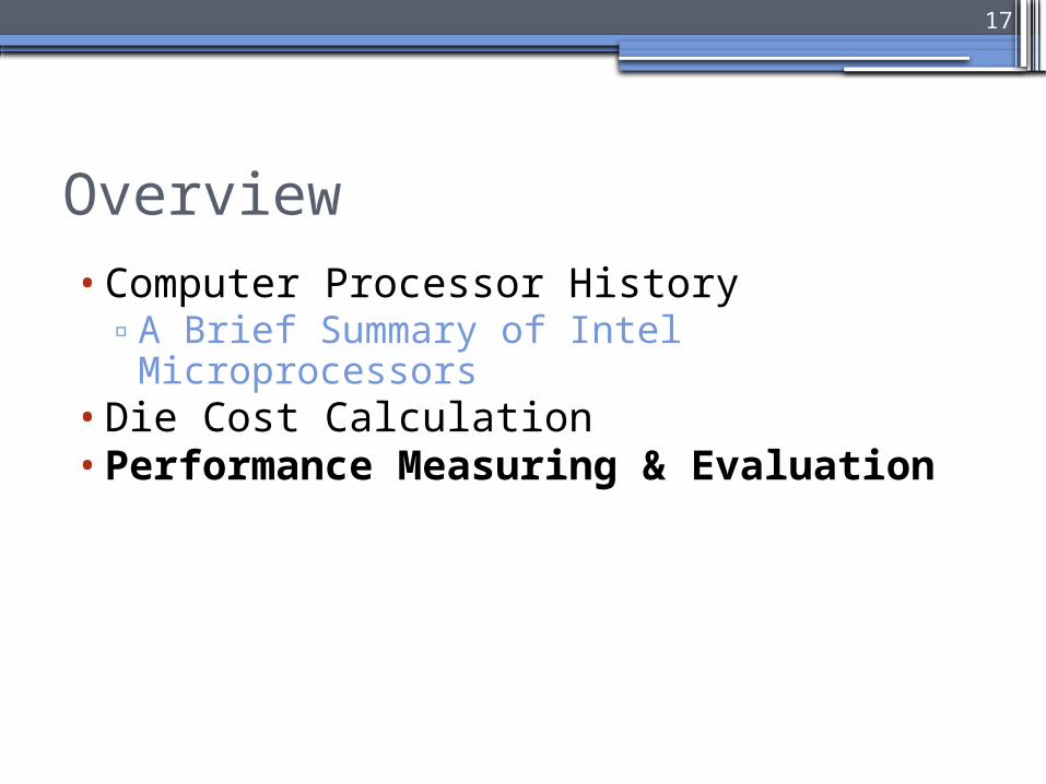
Overview•Computer Processor History

▫A Brief Summary of Intel Microprocessors

•Die Cost Calculation•Performance Measuring & Evaluation

2

• 4 bits processor

• 8 bits processors

Advances Come from Design- A Brief History of Intel Microprocessors

3

4004 (1971)• Intel's first microprocessor

8008 (1972)• twice as powerful as

the 4004

8080 (1974)• brains of the first personal

computer • ~US$ 400

8086 – 8088 (1978)• brains of IBM's new hit product -- the IBM PC• The 8088's success propelled Intel into the ranks of the

Fortune 500, and Fortune magazine named the company one of the "Business Triumphs of the Seventies." 80286 (1982)

• first Intel processor that could run all the software written for its predecessor

• Within 6 years of its release, an estimated 15 million 286-based personal computers were installed around the world.

• 16 bits processor

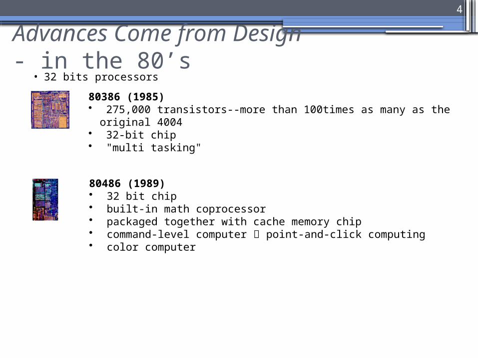
Advances Come from Design- in the 80’s

4

80386 (1985)• 275,000 transistors--more than 100times as many as the original

4004• 32-bit chip • "multi tasking"

80486 (1989)• 32 bit chip• built-in math coprocessor• packaged together with cache memory chip • command-level computer point-and-click computing• color computer

• 32 bits processors

4

Advances Come from Design- in the 90’s

5

Pentium Pro (1995)• 5.5 million transistors • packaged together with a second speed-enhancing cache

memory chip,• pipelining • enabling fast computer-aided design, mechanical engineering

and scientific computationPentium II (1997)• 7.5 million-transistor• MMX technology, designed specifically to process video,

audio and graphics data efficiently• high-speed cache memory chip

Celeron (1999)• excellent performance in gaming

Pentium (1993)• incorporate "real world" data such as speech, sound,

handwriting and photographic images

Advances Come from Design- in the Millenniums'

6

Pentium III (1999) • 9.5 million transistors, 0.25-micron technology • 70 new SSE (Streaming SIMD Extension) instructions• dramatically enhance the performance of advanced imaging,

3-D, streaming audio, video and speech recognition applications, Internet experiences

Pentium 4 (2000)• 42 million transistors and circuit lines of 0.18 microns• 1.5 gigahertz (4004 ran at 108 kilohertz )• SSE2 instructions, more pipeline stages, higher

successful prediction rate• can create professional-quality movies; deliver TV-like

video via the Internet; communicate with real-time video and voice; render 3D graphics in real time; quickly encode music for MP3 players; and simultaneously run several multimedia applications while connected to the Internet.

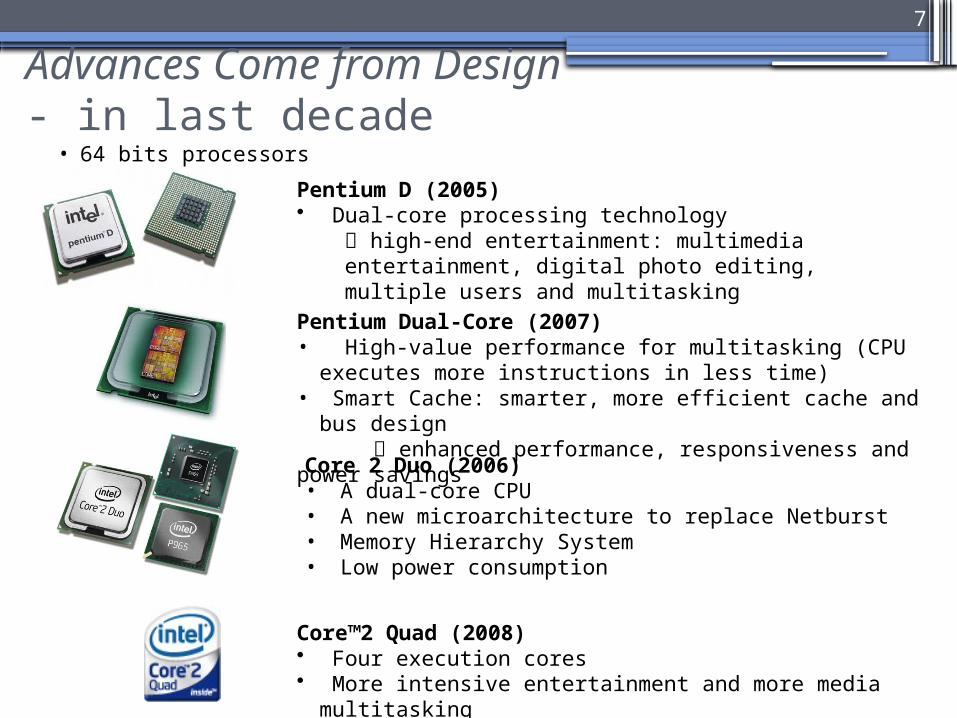
Advances Come from Design- in last decade

7

Pentium D (2005)• Dual-core processing technology

high-end entertainment: multimedia entertainment, digital photo editing, multiple users and multitasking

Pentium Dual-Core (2007)• High-value performance for multitasking (CPU executes

more instructions in less time)• Smart Cache: smarter, more efficient cache and bus

design enhanced performance, responsiveness and power savings Core 2 Duo (2006)• A dual-core CPU• A new microarchitecture to replace Netburst• Memory Hierarchy System• Low power consumption

Core™2 Quad (2008)• Four execution cores • More intensive entertainment and more media multitasking

• 64 bits processors

Advances Come from Design - Nowadays ( Consumer Level )

8

Core™2 i series (2008)• aims at

• Reducing idle power• Boosting performance by increasing processor

frequency• Hyper-threading

Core™2 i3 • A dual-core CPUCore™2 i5 • A quad-core CPUCore™2 i7 • A quad-core CPU (up to 8 cores)

Advances Come from Design - Nowadays ( Server Level )

9

Xeon SeriesThe Xeon is a brand of multiprocessing- or multi-socket-capable microprocessors designed and manufactured by Intel targeted at the non-consumer workstation, server, embedded systems markets.

E3 series "Sandy Bridge“• Quad-core, enables  ECC memory

E5 v2 series "Ivy Bridge• Hexa-core to Eight-core

E5 v3-series "Haswell"• Up to 14 cores inside. Latest

Architecture, better energy efficiency and CPU speed

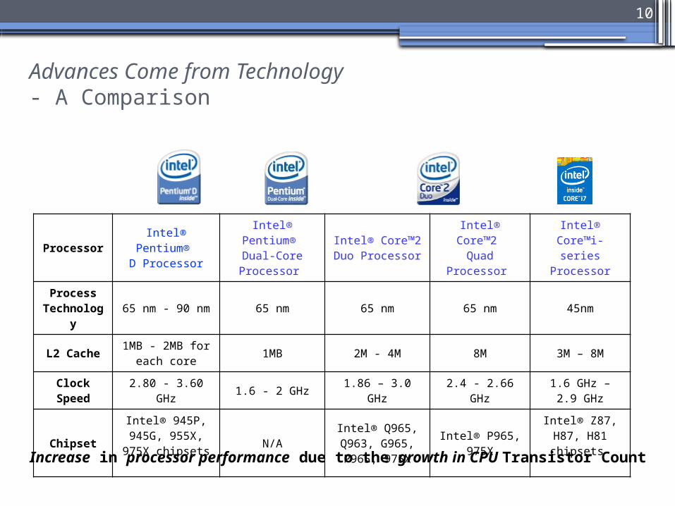
Advances Come from Technology- A Comparison

10

ProcessorIntel®

Pentium® D Processor

Intel® Pentium® Dual-Core Processor

Intel® Core™2 Duo Processor

Intel® Core™2 Quad

Processor

Intel® Core™i-series

Processor

Process Technolog

y65 nm - 90 nm 65 nm 65 nm 65 nm 45nm

L2 Cache1MB - 2MB for

each core1MB 2M - 4M 8M 3M – 8M

Clock Speed

2.80 - 3.60 GHz 1.6 - 2 GHz 1.86 – 3.0 GHz 2.4 - 2.66 GHz1.6 GHz – 2.9

GHz

Chipset

Intel® 945P, 945G, 955X,

975X chipsetsN/A

Intel® Q965, Q963, G965, P965, 975X

Intel® P965, 975X

Intel® Z87, H87, H81 chipsets

Increase in processor performance due to the growth in CPU Transistor Count

Overview•Computer Processor History

▫A Brief Summary of Intel Microprocessors•Die Cost Calculation•Performance Measuring & Evaluation

11

Cost of an Integrated Circuit

12

Where α is a parameter inversely proportional to the number of maskLevels, which is a measure of the manufacturing complexity.For today’s CMOS process, good estimate is α = 3.0 – 4.0

Yield: the percentage of manufactured devices that survives the testing procedure

wafer

die

YieldTest Final

Cost PackagingCost TestingCost DieCost IC

Yield DieWaferDies

CostWafer Cost Die

21

2

AreaDie2

diameterWafer

AreaDie

2diameterWafer Waferper Dies

AreaDieareaunit per Defects

1YieldWafer Yield Dies

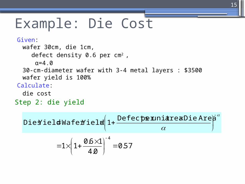
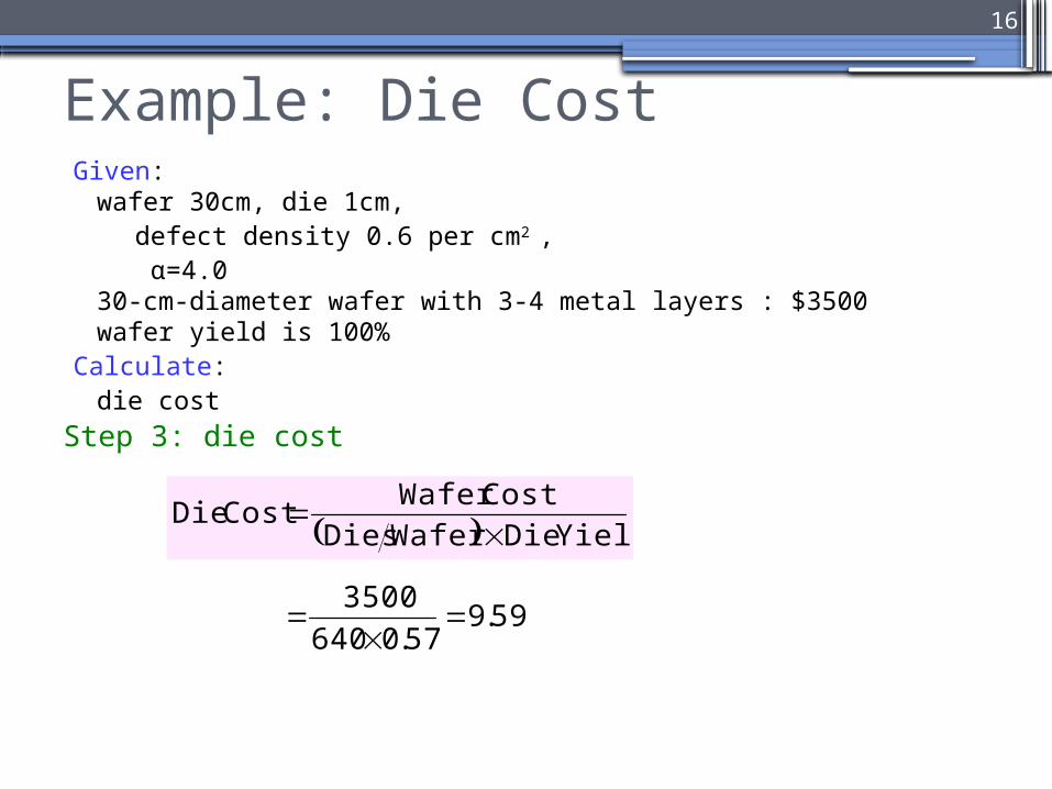
Example: Die CostGiven:

wafer 30cm, die 1cm, defect density 0.6 per cm2 , α=4.0

30-cm-diameter wafer with 3-4 metal layers : $3500wafer yield is 100%

Calculate: die cost

13

To calculate the die cost,

- Given wafer cost- Dies/Wafer?- Die Yield?

Yield DieWaferDies

CostWafer Cost Die

Example: Die CostGiven:

wafer 30cm, die 1cm, defect density 0.6 per cm2 , α=4.0

30-cm-diameter wafer with 3-4 metal layers : $3500wafer yield is 100%

Calculate: die cost

640112

30

11

)2/30( 2

14

Step 1: dies per wafer

21

2

AreaDie2

diameterWafer

AreaDie

2diameterWafer Waferper Dies

Example: Die CostGiven:

wafer 30cm, die 1cm, defect density 0.6 per cm2 , α=4.0

30-cm-diameter wafer with 3-4 metal layers : $3500wafer yield is 100%

Calculate: die cost

15

57.00.4

16.011

4

Step 2: die yield

AreaDieareaunit per Defects

1YieldWafer Yield Dies

Example: Die CostGiven:

wafer 30cm, die 1cm, defect density 0.6 per cm2 , α=4.0

30-cm-diameter wafer with 3-4 metal layers : $3500wafer yield is 100%

Calculate: die cost

16

Step 3: die cost

59.957.0640

3500

Yield DieWaferDies

CostWafer Cost Die

Overview•Computer Processor History

▫A Brief Summary of Intel Microprocessors•Die Cost Calculation•Performance Measuring & Evaluation

17

How to Measure Performance ?•Performance Rating

▫CPU Time▫Benchmark programs

Integer programs and floating point programsCompressionCompilerArtificial IntelligencePhysics / Quantum ComputingVideo CompressionPath-finding Algorithms

▫Comparing & Summarizing Performance▫Amdahl’s Law

18

Measuring Performance- CPU Execution Time

•Performance = 1 / Execution Time

19

CPU time = Seconds = Instructions x Cycles x Seconds

Program Program Instruction Cycle

CPU time = Seconds = Instructions x Cycles x Seconds

Program Program Instruction Cycle

Clock cycle = 1 / Clock

rate

CPIInstructioncount

Measuring CPU Time – Example 1

20

A SPEC CPU2006 integer benchmark (464.h264ref, a video compression program written in C) is run on a Pentium D processor:

Total instruction count: 3731 billionAverage CPI for the program: 2.5 cycles/instruction.CPU clock rate: 2.1 GHz

CPU time = Instruction count x CPI x (1/clock rate)

Source: Analysis of Redundancy and Application Balance in the SPEC CPU2006 Benchmark Suite

CPU time = 3731 x 109 x 2.5 / (2.1 x 109) = 4442 seconds

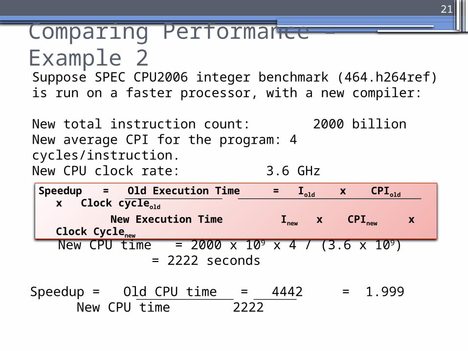
Suppose SPEC CPU2006 integer benchmark (464.h264ref) is run on a faster processor, with a new compiler:

New total instruction count: 2000 billionNew average CPI for the program: 4 cycles/instruction.New CPU clock rate: 3.6 GHz

Speedup = Old CPU time = 4442 = 1.999New CPU time 2222

Comparing Performance – Example 2

21

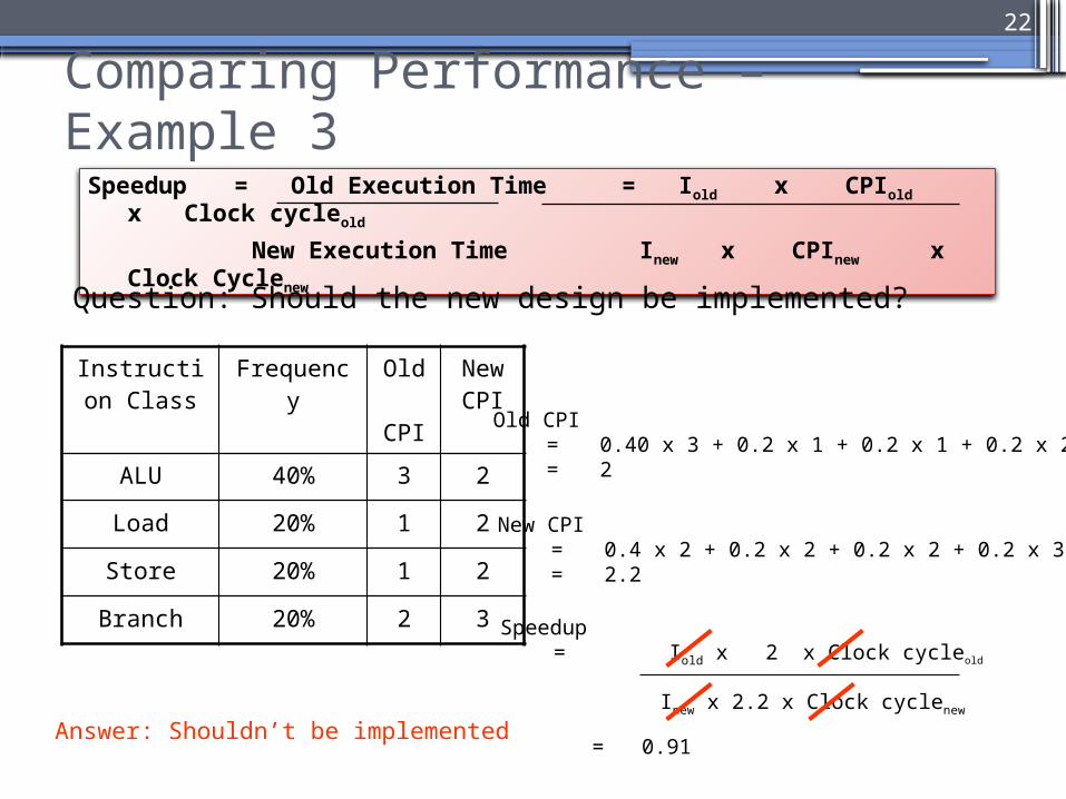
Speedup = Old Execution Time = Iold x CPIold x Clock cycleold

New Execution Time Inew x CPInew x Clock Cyclenew

New CPU time = 2000 x 109 x 4 / (3.6 x 109) = 2222 seconds

Comparing Performance – Example 3

Instruction Class

Frequency Old CPI

New CPI

ALU 40% 3 2

Load 20% 1 2

Store 20% 1 2

Branch 20% 2 3

22

Speedup = Old Execution Time = Iold x CPIold x Clock cycleold

New Execution Time Inew x CPInew x Clock Cyclenew

Question: Should the new design be implemented?

Speedup = Iold x 2 x Clock cycleold

Inew x 2.2 x Clock cyclenew

Answer: Shouldn’t be implemented

Old CPI = 0.40 x 3 + 0.2 x 1 + 0.2 x 1 + 0.2 x 2= 2

New CPI = 0.4 x 2 + 0.2 x 2 + 0.2 x 2 + 0.2 x 3= 2.2

= 0.91

Metrics for PerformanceCPU time: most accurate and fair measure

23

CPU Time = Instruction Count x CPI x Clock Cycle Time

n

i 1ii ICCPIcyclesclock CPU

n

iiFCPI

1iCPI a priori frequency of the

instruction set

• Suppose we have made the following measurements:Frequency of FP operations (other than FPSQR) = 23%Average CPI of FP operations (other than FPSQR) = 4.0Frequency of FPSQR = 2%, CPI of FPSQR = 20Average CPI of other instructions = 1.33

• Assume that the two design alternatives▫ decrease the CPI of FPSQR to 3▫ decrease the average CPI of FP operations (other than

FPSQR) to 2.

• Compare these two design alternatives using the CPU performance equation.

24

Measuring Performance – Example 4

SolutionStep 1: Original CPI without enhancement: CPI original = 423% + 20x2% +1.3375% = 2.3175

Step 2: compute the CPI for the enhanced FPSQR by subtracting the cycles saved from the original CPI:

CPI with new FPSQR = CPI original - 2%(CPI old FPSQR – CPI new FPSQR only) = 2.3175 - 0.02x(20-3) = 1.9775

Step 3: compute the CPI for the enhancement of all FP instructions:CPI with new FP = CPI original - 23%(CPI old FP – CPI new FP)

= 2.3175 - 0.23x(4-2) = 1.8575

Step 4: the speedup for the FP enhancement over FPSQR enhancement is:Speedup = CPU time with new FPSQR / CPU time with new FP

= (I CPI with new FPSQR C) / (I CPI with new FP C) = CPI with new FPSQR / CPI with new FP = 1.9775 / 1.8575 = 1.065

25

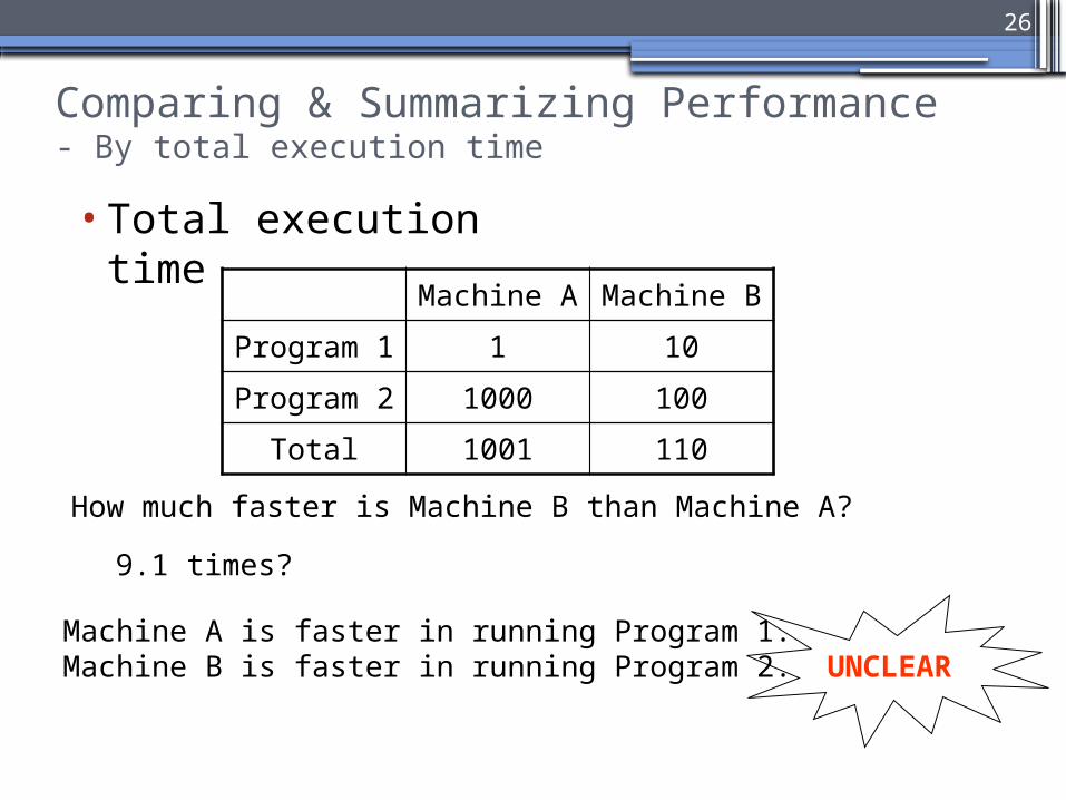
Comparing & Summarizing Performance - By total execution time

•Total execution time

Machine A Machine B

Program 1 1 10

Program 2 1000 100

Total 1001 110

26

How much faster is Machine B than Machine A?

9.1 times?

Machine A is faster in running Program 1.Machine B is faster in running Program 2. UNCLEAR

Comparing & Summarizing Performance- by arithmetic mean of execution time

Machine A

Machine B

Program 1

1 10

Program 2

1000 100

Total 1001 110

AM 500.5 55

Machine A

Machine B

Program 1

200 400

Program 2

250 400

Program 3

450 100

AM 300 300

27

Arithmetic Mean: nS Execution Timei

i=1

1

n

Can be misleading

Valid only if programs run

equally

Comparing & Summarizing Performance- by weighted arithmetic mean of execution time

Machine A Machine B W (1)

Program 1

200 400 0.4

Program 2

250 500 0.4

Program 3

550 100 0.2

AM 300 300

WAM (1) 200 x 0.4 + 250 x 0.4 + 550 x 0.2 = 290

400 x 0.4 + 500 x 0.4 + 100 x 0.2 = 380

28

Weighted Arithmetic Mean: nS Weighti x Execution Timei

i=1

Machine A is better

For the 1st of Weights:

Comparing & Summarizing Performance- by weighted arithmetic mean of execution time

Machine A Machine B W (2)

Program 1

200 400 0.2

Program 2

250 500 0.2

Program 3

550 100 0.6

AM 300 300

WAM (2) 200 x 0.2 + 250 x 0.2 + 550 x 0.6 = 420

400 x 0.2 + 500 x 0.2 + 100 x 0.6 = 240

29

Weighted Arithmetic Mean: nS Weighti x Execution Timei

i=1

Machine B is better

It depends very much on how to weigh each testing item

For the 2nd set of Weights:

Comparing & Summarizing Performance- by geometric mean of execution time

Machine A

Machine B

Program 1

1 10

Program 2

1000 100

Total 1001 110

Normalized to A

Machine A

Machine B

Program 1 1 10

Program 2 1 0.1

GM 1 1

30

Geometric Mean: nP Execution time ratioiI=1

n

Normalized Execution Time to a reference machine

Same GM ≠

same execution time or same performance

n

n

in

n

i

n

n

in

n

i

n

n

i

ieBPerformanc

ieAPerformanc

iimeAExecutionT

iimeBExecutionT

iSPECRatioB

iSPECRatioA

iSPECRatioB

iSPECRatioA

BeanGeometricM

AeanGeometricM

11

1

1

1

References:

• John L. Hennessy and David A. Patterson. Computer Architecture: A Quantitative Approach. Morgan Kaufman Publishers, 5th Edition, 2011

• Intel▫ http://www.intel.com▫ http://www.intel.com/content/www/us/en/history/museum-stor

y-of-intel-4004.html▫ http://www.intel.com/pressroom/kits/quickrefyr.htm

• Timeline of Microprocessor http://m.theinquirer.net/inquirer/feature/2124781/microprocessor-development

31

Appendix : Amdahl’s Law

...SF

SF...)FF(

22

11211

1

tEnhancemen With TimeExecution t Enhancemen Without TimeExecution Speedupoverall

32

• Amdahl’s Law – law of diminishing returns• In general case, assume several enhancements has been

taken for the system, the speedup for whole system is:

where Fi is the fraction of enhancement i and Si is the speedup of the corresponding enhancement

• The new execution time is

ii enhancedi

enhanced ienhanced ioldnew Speedup

Fraction)Fraction-1(timeExecution timeExecution

Amdahl’s Law - An Example

• Float instruction: ▫ Fraction: 50%▫ Speedup: 2.0x

• Integer instruction:▫ Fraction: 30%▫ Speedup: 3.0x

• Others keep the same.

ii enhancedi

enhanced ienhanced i Speedup

Fraction)Fraction-1(

1 Speedup

33

= 1 / ((1-0.5-0.3)+(0.5/2+0.3/3))=1.818

Amdahl’s Law - Intuition: “Make the common case faster”

• I have two processors, which can help accelerate one of the below parts by parallel processing. Two parts occupy the total time percentage of 95% and 5%.

• Fractionenhanced = 95%, Speedupenhanced = 2.0xSpeedupoverall = 1/((1-0.95)+0.95/2) = 1.905

• Fractionenhanced = 5%, Speedupenhanced = 2.0xSpeedupoverall = 1/((1-0.05)+0.05/2) = 1.026

1.905 vs. 1.026 Make the common case faster!!

• Fractionenhanced = 5%, Speedupenhanced -> infinitySpeedupoverall = 1/(1-0.05) = 1.052

1.052 is still much smaller than 1.905.

34

A Common Confusion: CPI vs. Amdahl’s Law

• Assume a program consists of three classes of instructions A,B and C, as shown below.

• An enhancement is made by doubling the speed of instruction class A

• Assume instruction count for the program and CPU clock cycle is not influenced

• What is the overall speedup achieved for the program

Instruction

Class

Frequency

Old CPI

NewCPI

A 20% 2 1

B 20% 3 3

C 60% 4 4

35

1.0625

CycleClock ICCPI

CycleClock ICCPI

timeExecution

timeExecution

2.346.032.012.0

4.346.032.022.0

new

old

new

old

overall

new

old

Speedup

CPI

CPI

Method 1: CPI

Method 2: Amdahl’s Law

111.1

2%20

%)201(

1

overallSpeedup

The fraction in Amdahl’s law is time fractionMethod 2: Amdahl’s Law

0625.1

211764.0

)11764.01(

1

11764.0%604%203%202

20%2 A offraction Time

overallSpeedup