Embed Size (px)
Citation preview
Markus [email protected]
FEEG6017 lecture:Relationship between two variables: correlation, covariance and r-squared
Relationships between variables
• So far we have looked at ways of characterizing the distribution of a single variable, and testing hypotheses about the population based on a sample.
• We're now moving on to the ways in which two variables can be examined together.
• This comes up a lot in research!
Relationships between variables
• You might want to know:o To what extent the change in a patient's blood
pressure is linked to the dosage level of a drug they've been given.
o To what degree the number of plant species in an ecosystem is related to the number of animal species.
o Whether temperature affects the rate of a chemical reaction.
Relationships between variables
• We assume that for each case we have at least two real-valued variables.
• For example: both height (cm) and weight (kg) recorded for a group of people.
• The standard way to display this is using a dot plot or scatterplot.
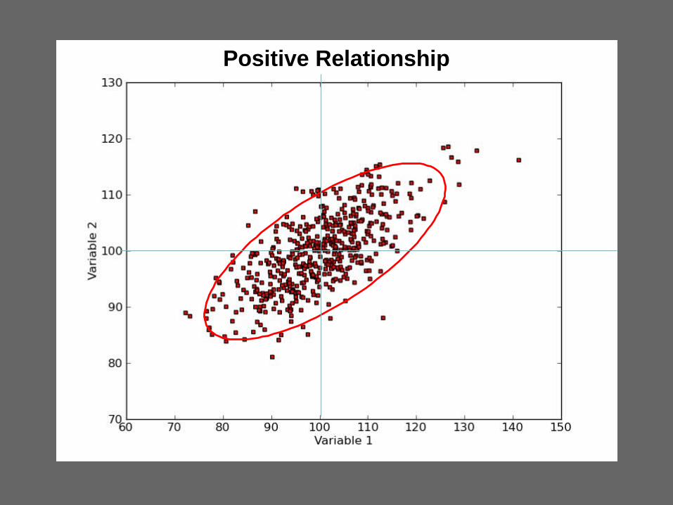
Positive Relationship
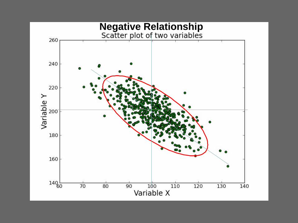
Negative Relationship

No Relationship

Measuring relationships?
• We're going to need a way of measuring whether one variable changes when another one does.
• Another way of putting it: when we know the value of variable A, how much information do we have about variable B's value?
Recap of the one-variable case
• Perhaps we can borrow some ideas about the way we characterized variation in the single-variable case.
• With one variable, we start out by finding the mean, which is also the expectation of the distribution.
Sum of the squared deviations
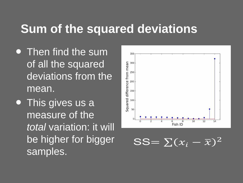
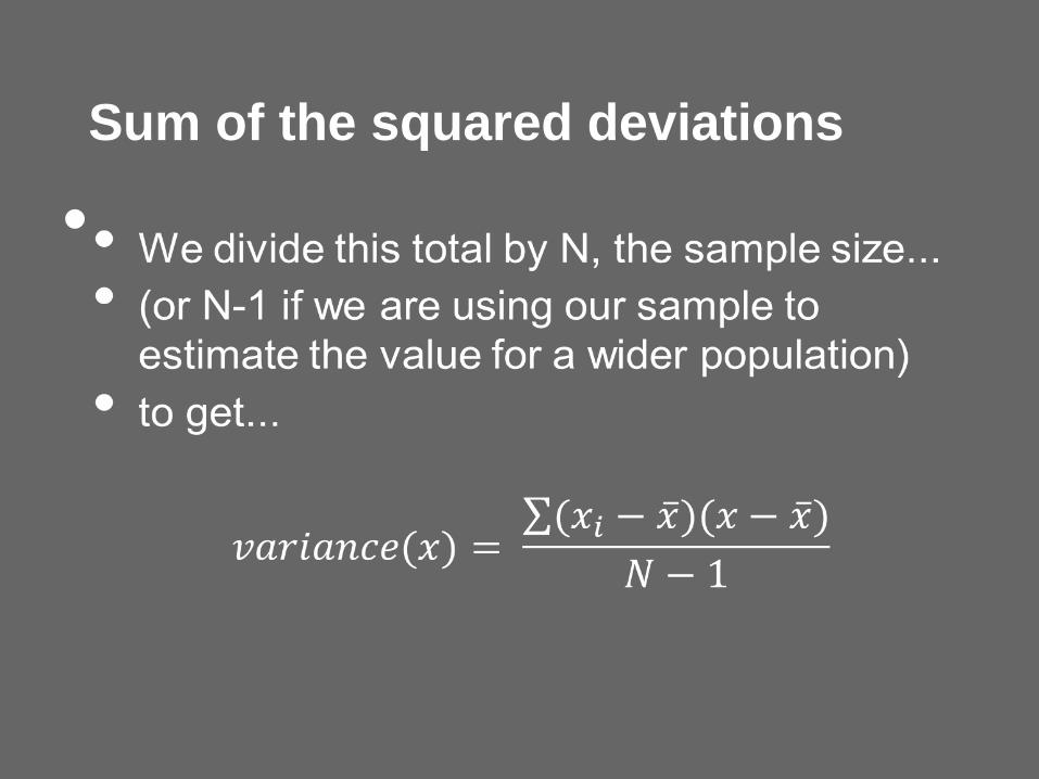
• Then find the sum of all the squared deviations from the mean.
• This gives us a measure of the total variation: it will be higher for bigger samples.
Sum of the squared deviations
•
The variance
• This is a good measure of how much variation exists in the sample, normalized by sample size.
• It has the nice property of being additive.
• The only problem is that the variance is measured in units squared.
• So we take the square root to get...
The standard deviation
•
The standard deviation
• With a good estimate of the population SD, we can reason about the standard deviation of the distribution of sample means.
• That's a number that gets smaller as the sample sizes get bigger.
• To calculate this from the sample standard deviation we divide through by the square root of N, the sample size, to get...
The standard error
• This measures the precision of our estimation of the true population mean.
• Plus or minus 1.96 standard errors from the sample mean should capture the true population mean 95% of the time.
• The standard error is itself the standard deviation of the distribution of the sample means.
Variation in one variable
• So, these four measures all describe aspects of the variation in a single variable:a. Sum of the squared deviations
b. Variance
c. Standard deviation
d. Standard error
• Can we adapt them for thinking about the way in which two variables might vary together?
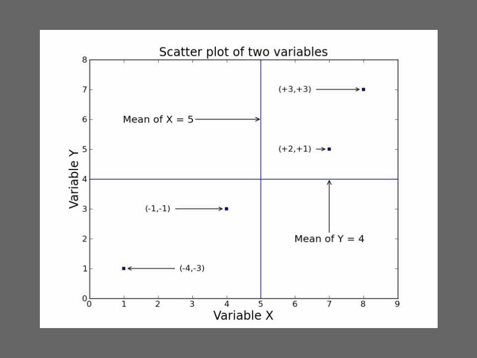
Two variable example
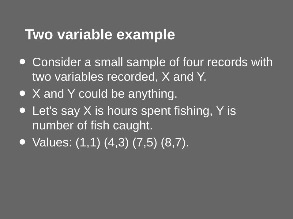
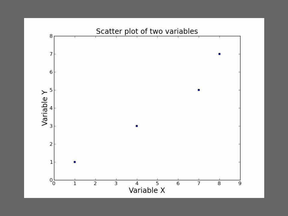
• Consider a small sample of four records with two variables recorded, X and Y.
• X and Y could be anything.
• Let's say X is hours spent fishing, Y is number of fish caught.
• Values: (1,1) (4,3) (7,5) (8,7).
Two variable example
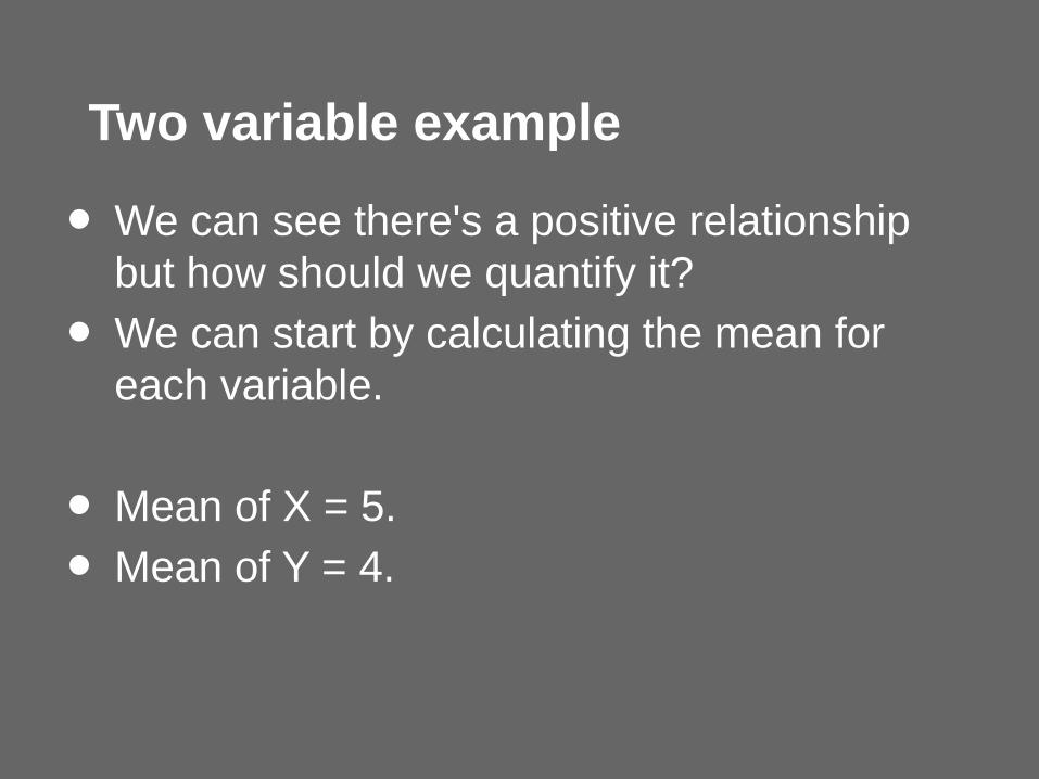
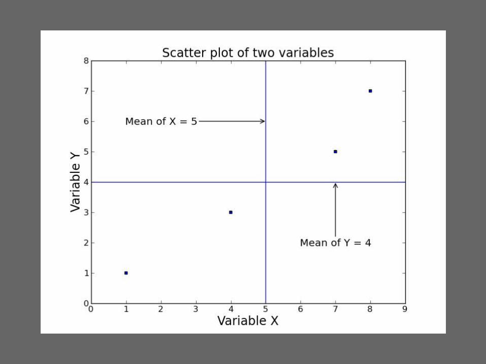
• We can see there's a positive relationship but how should we quantify it?
• We can start by calculating the mean for each variable.
• Mean of X = 5.
• Mean of Y = 4.
Two variable example
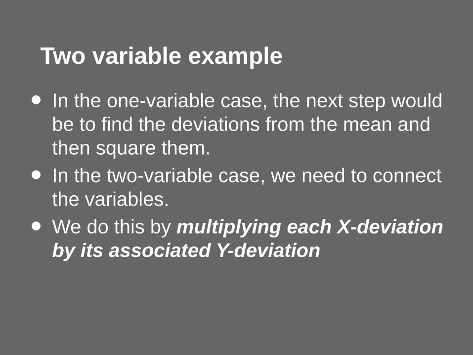
• In the one-variable case, the next step would be to find the deviations from the mean and then square them.
• In the two-variable case, we need to connect the variables.
• We do this by multiplying each X-deviation by its associated Y-deviation
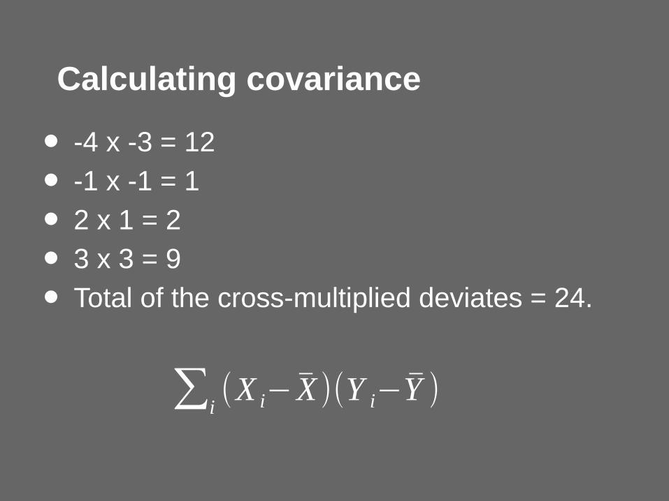
Calculating covariance
• -4 x -3 = 12
• -1 x -1 = 1
• 2 x 1 = 2
• 3 x 3 = 9
• Total of the cross-multiplied deviates = 24.
∑i(X i− X )(Y i−Y )
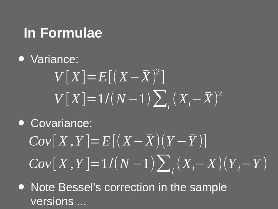
In Formulae
• Variance:
• Covariance:
• Note Bessel's correction in the sample versions ...
V [X ]=1/(N−1)∑i(X i− X )2
Cov [X ,Y ]=1 /(N−1)∑i(X i− X )(Y i−Y )
V [X ]=E [(X−X )2]
Cov [X ,Y ]=E [(X− X )(Y−Y )]
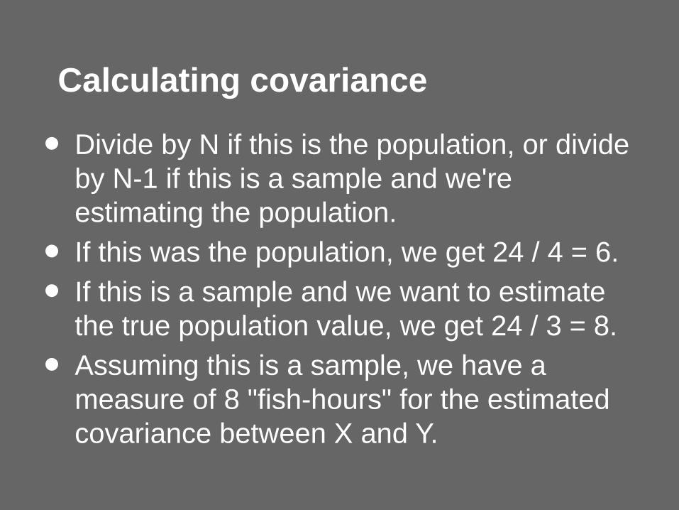
Calculating covariance
• Divide by N if this is the population, or divide by N-1 if this is a sample and we're estimating the population.
• If this was the population, we get 24 / 4 = 6.
• If this is a sample and we want to estimate the true population value, we get 24 / 3 = 8.
• Assuming this is a sample, we have a measure of 8 "fish-hours" for the estimated covariance between X and Y.
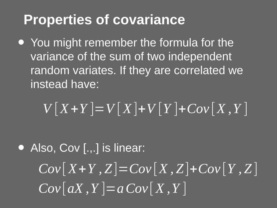
Properties of covariance
• You might remember the formula for the variance of the sum of two independent random variates. If they are correlated we instead have:
• Also, Cov [.,.] is linear:
V [X+Y ]=V [X ]+V [Y ]+Cov [X ,Y ]
Cov [X+Y , Z ]=Cov [X , Z ]+Cov [Y , Z ]
Cov [aX ,Y ]=aCov [X ,Y ]
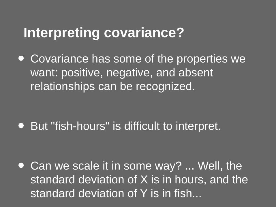
Interpreting covariance?
• Covariance has some of the properties we want: positive, negative, and absent relationships can be recognized.
• But "fish-hours" is difficult to interpret.
• Can we scale it in some way? ... Well, the standard deviation of X is in hours, and the standard deviation of Y is in fish...
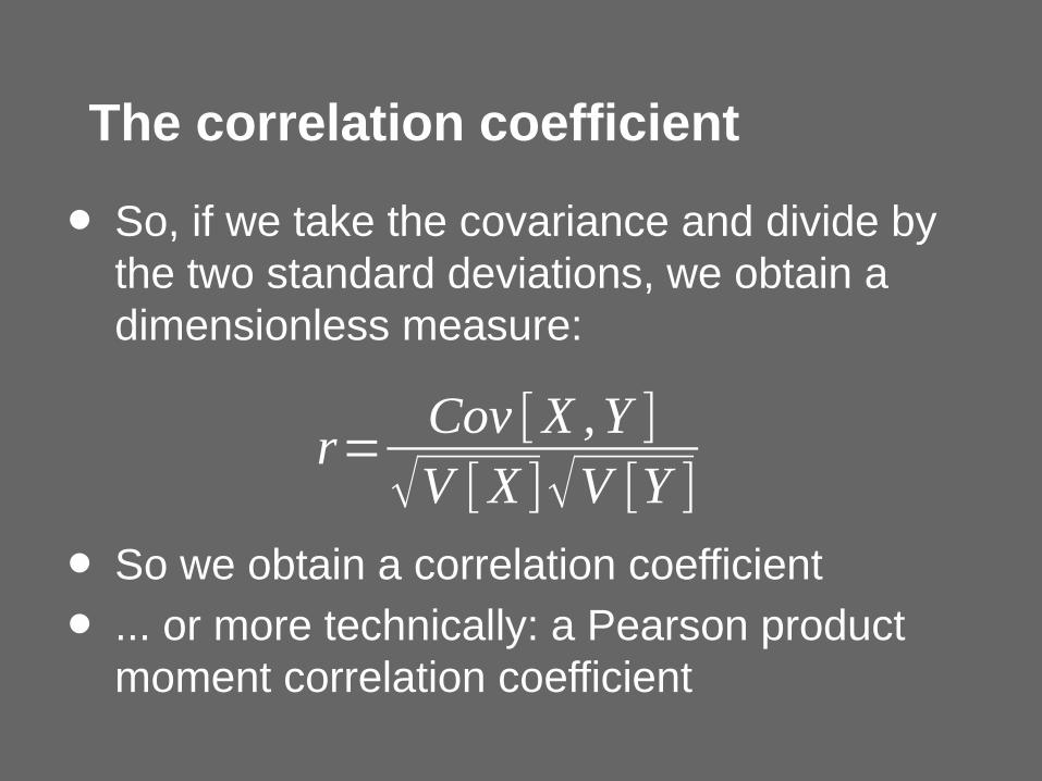
The correlation coefficient
• So, if we take the covariance and divide by the two standard deviations, we obtain a dimensionless measure:
• So we obtain a correlation coefficient
• ... or more technically: a Pearson product moment correlation coefficient
r=Cov [X ,Y ]
√V [X ]√V [Y ]
The correlation coefficient
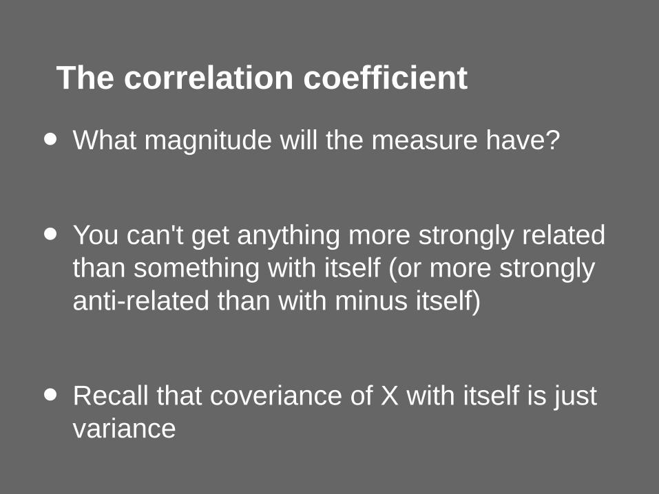
• What magnitude will the measure have?
• You can't get anything more strongly related than something with itself (or more strongly anti-related than with minus itself)
• Recall that coveriance of X with itself is just variance
The correlation coefficient
• This measure runs between -1 and 1, and represents negative, absent, and positive relationships.
• It's often referred to as "r".
• It's extremely popular as a way of measuring the strength of a linear relationship.
The correlation coefficient
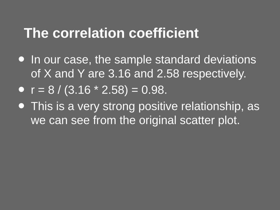
• In our case, the sample standard deviations of X and Y are 3.16 and 2.58 respectively.
• r = 8 / (3.16 * 2.58) = 0.98.
• This is a very strong positive relationship, as we can see from the original scatter plot.
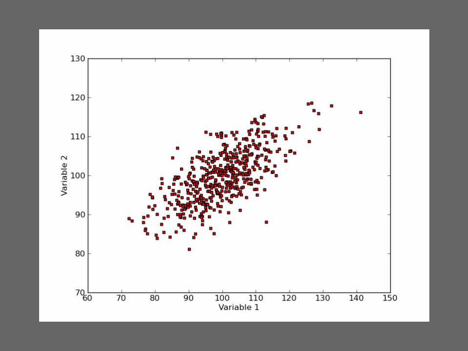
Another example
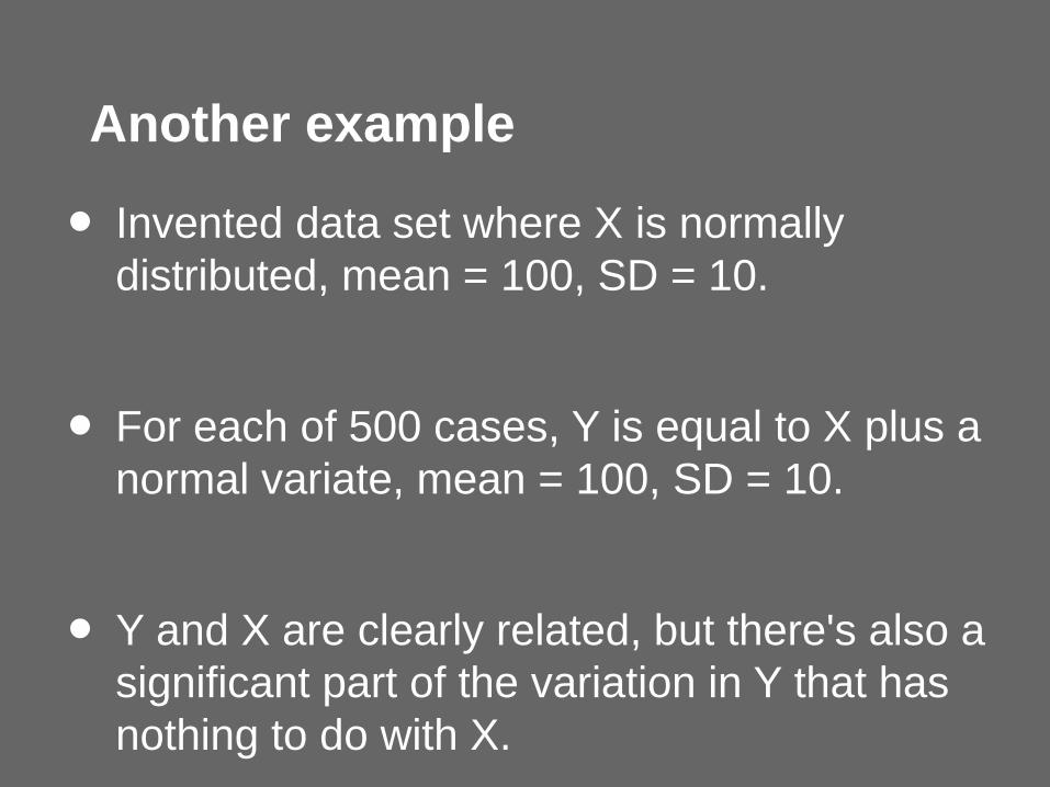
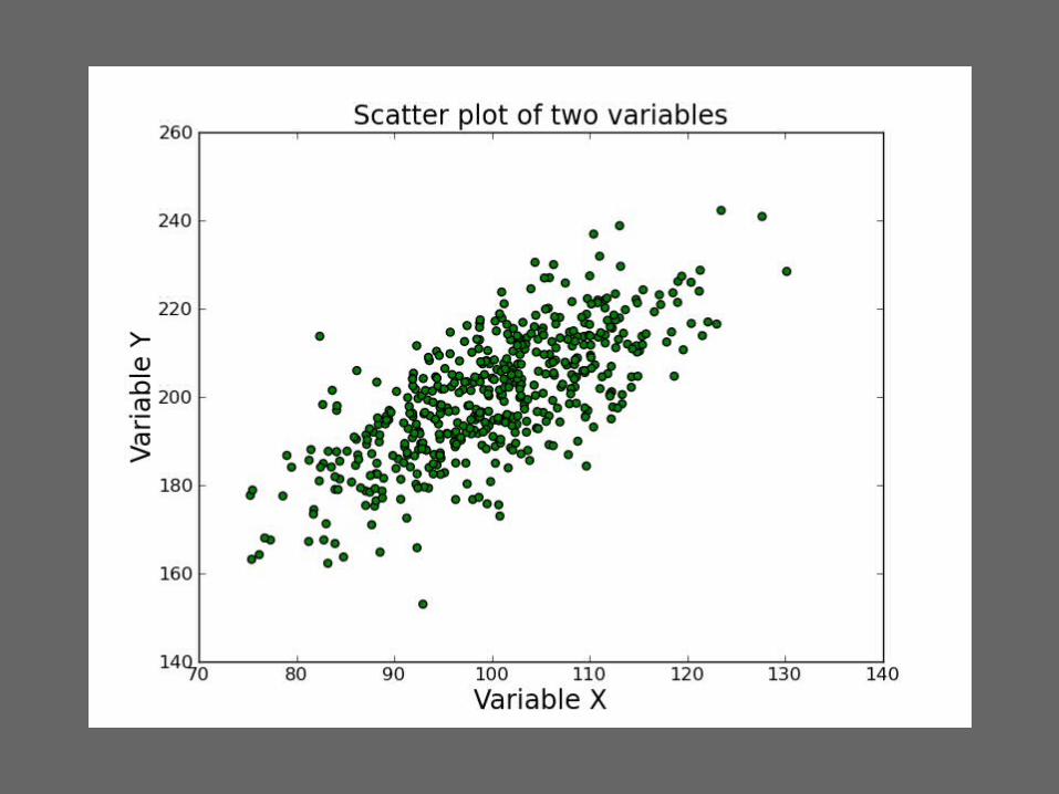
• Invented data set where X is normally distributed, mean = 100, SD = 10.
• For each of 500 cases, Y is equal to X plus a normal variate, mean = 100, SD = 10.
• Y and X are clearly related, but there's also a significant part of the variation in Y that has nothing to do with X.
Calculating the correlation coefficient
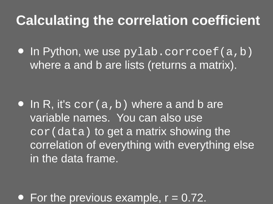
• In Python, we use pylab.corrcoef(a,b) where a and b are lists (returns a matrix).
• In R, it's cor(a,b) where a and b are variable names. You can also use cor(data) to get a matrix showing the correlation of everything with everything else in the data frame.
• For the previous example, r = 0.72.
Interpreting correlation coefficients
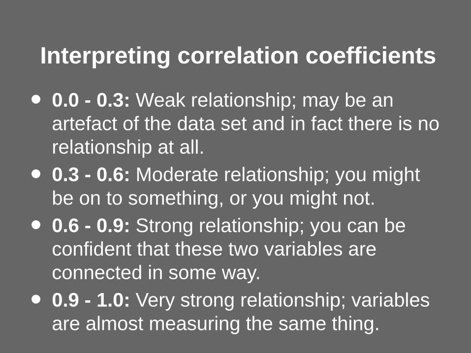
• 0.0 - 0.3: Weak relationship; may be an artefact of the data set and in fact there is no relationship at all.
• 0.3 - 0.6: Moderate relationship; you might be on to something, or you might not.
• 0.6 - 0.9: Strong relationship; you can be confident that these two variables are connected in some way.
• 0.9 - 1.0: Very strong relationship; variables are almost measuring the same thing.
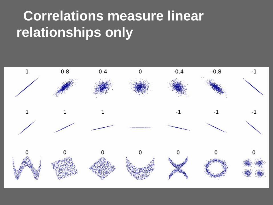
Correlations measure linear relationships only
Correlation is not causality
• Of course, just because X and Y are correlated does not mean that X causes Y.
• They could both be caused by some other factor Z.
• Y might cause X instead.
• Low correlations might result from no causal linkage, just sampling noise.
Range effects
• Two variables can be strongly related across the whole of their range, but with no strong relationship in a limited subset of that range.
• Consider the relationship between price and top speed in cars: broadly positive.
• But if we look only at very expensive cars, the two values may be uncorrelated.
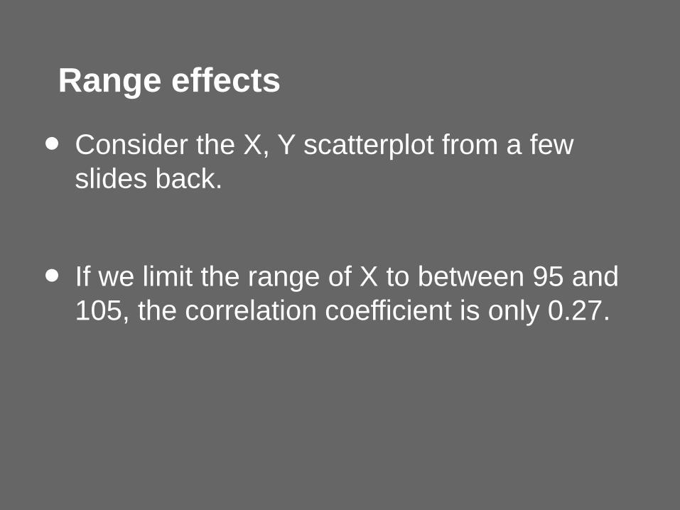
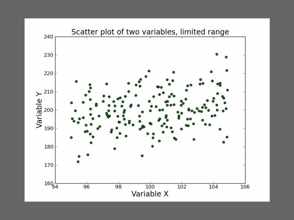
Range effects
• Consider the X, Y scatterplot from a few slides back.
• If we limit the range of X to between 95 and 105, the correlation coefficient is only 0.27.
Confidence intervals
• Confidence intervals for correlation coefficients can be calculated in much the same way as for means.
• As an exercise: using the Python code for this lecture, try drawing samples of size 50 repeatedly from the X, Y distribution and look at the range of values for r you get.
Permutation tests
• Another method is via permutation tests. This is a way to judge noise from small sample sizes.
• Take the data for (Xi,Y
i) and consider
permutations (Xi, Y
i). You can treat them as a
sample which gives you a null hypothesis.
• Last step is to test whether your actual data is likely to have been drawn from the sample.
Information about Y from X
• If I know the correlation between two things, what does knowing one thing tell me about the value of the other?
• Consider the X, Y example. X was a random variable, and Y was equal to X plus another random variable from the same distribution.
• The correlation worked out at about 0.7. Why?
R-squared
• Turns out that if we square the correlation coefficient we get a direct measure of the proportion of the variance explained.
• In our example case we know that X explains exactly 50% of the variance in Y.
• The square root of 0.5 ≈ 0.71.
R-squared
• r = 0.3 explains 9% of the variance.
• r = 0.6 explains 36% of the variance.
• r = 0.9 explains 81% of the variance.
• "R-squared" is a standard way of measuring the proportion of variance we can explain in one variable using one or more other variables. This connects with the next lecture on ANOVA.
Python code
• The Python code used to produce the graphs and correlation coefficients in this lecture is available here.