COMP9444 Neural Networks and Deep Learning 3 ...cs9444/17s2/lect/1page/03...COMP9444 Neural Networks and Deep Learning 3. Backpropagation Textbook, Sections 4.3, 5.2, 6.5.2 COMP9444

COMP9444Neural Networks and Deep Learning

3. Backpropagation

Textbook, Sections 4.3, 5.2, 6.5.2

COMP9444 c©Alan Blair, 2017

COMP9444 17s2 Backpropagation 1

Outline

� Supervised Learning

� Ockham’s Razor (5.2)

� Multi-Layer Networks

� Gradient Descent (4.3, 6.5.2)



Types of Learning

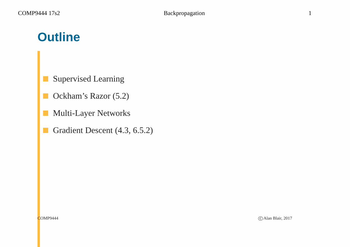
� Supervised Learning

◮ agent is presented with examples of inputs and their target outputs

� Reinforcement Learning

◮ agent is not presented with target outputs, but is given a reward

signal, which it aims to maximize

� Unsupervised Learning

◮ agent is only presented with the inputs themselves, and aimsto

find structure in these inputs



Supervised Learning

� we have atraining setand atest set, each consisting of a set of items;

for each item, a number of input attributes and a target valueare

specified.

� the aim is to predict the target value, based on the input attributes.

� agent is presented with the input and target output for each item in the

training set; it must then predict the output for each item inthe test set

� various learning paradigms are available:

◮ Neural Network

◮ Decision Tree

◮ Support Vector Machine, etc.



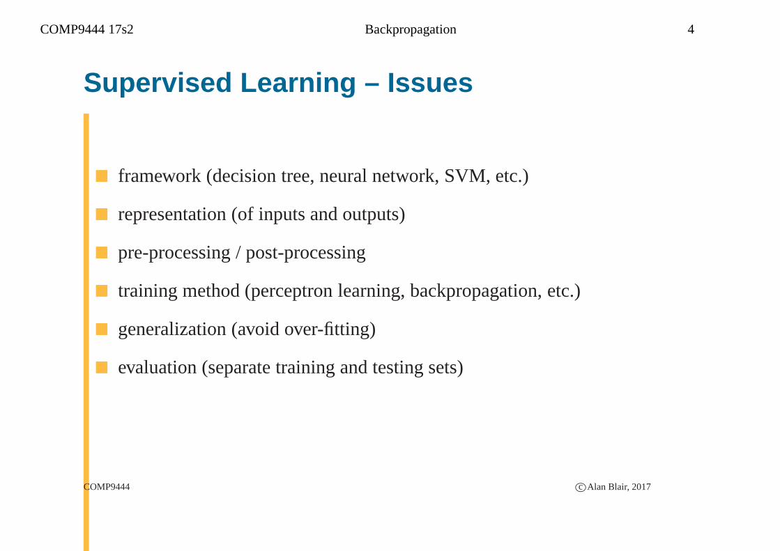
Supervised Learning – Issues

� framework (decision tree, neural network, SVM, etc.)

� representation (of inputs and outputs)

� pre-processing / post-processing

� training method (perceptron learning, backpropagation, etc.)

� generalization (avoid over-fitting)

� evaluation (separate training and testing sets)



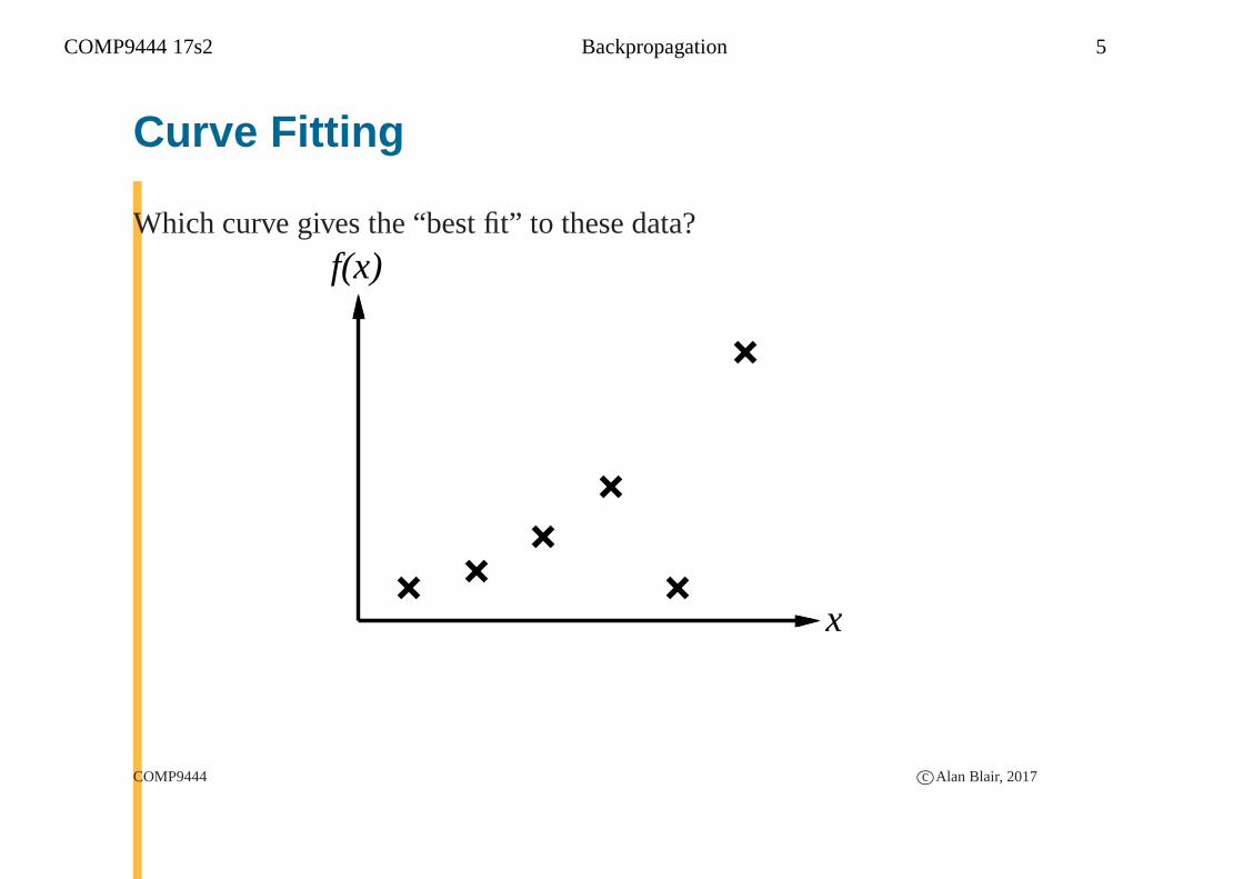
Curve Fitting

Which curve gives the “best fit” to these data?

x

f(x)



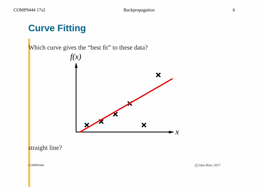
Curve Fitting


x

f(x)

straight line?



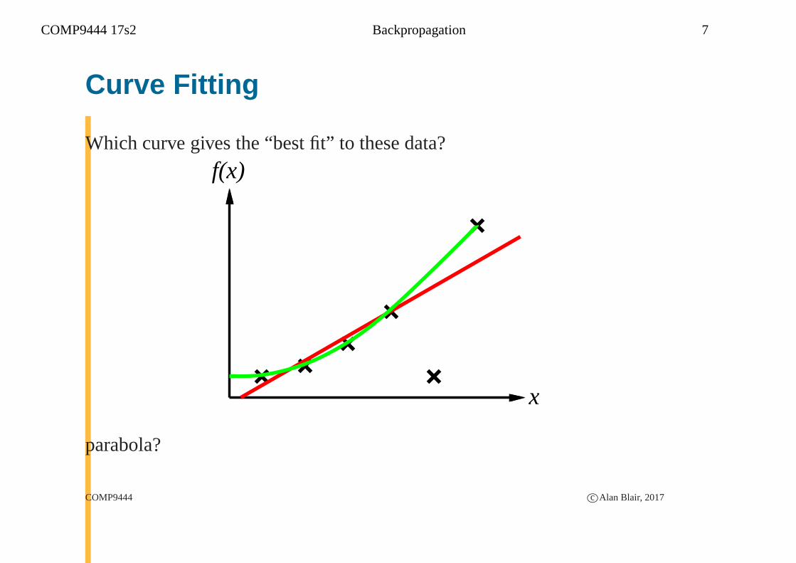
Curve Fitting


x

f(x)

parabola?



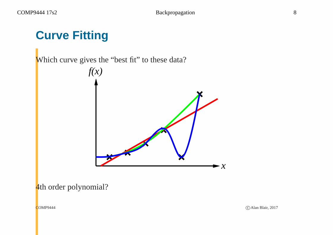
Curve Fitting


x

f(x)

4th order polynomial?



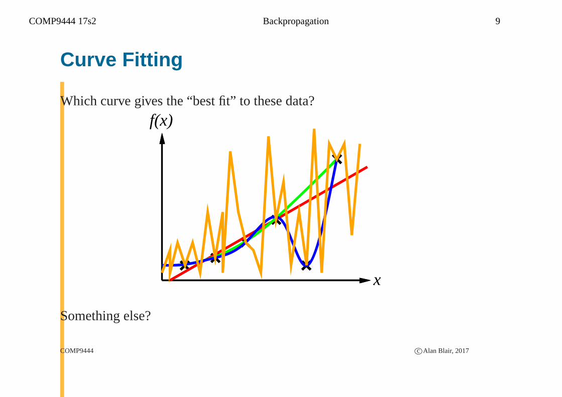
Curve Fitting


x

f(x)

Something else?



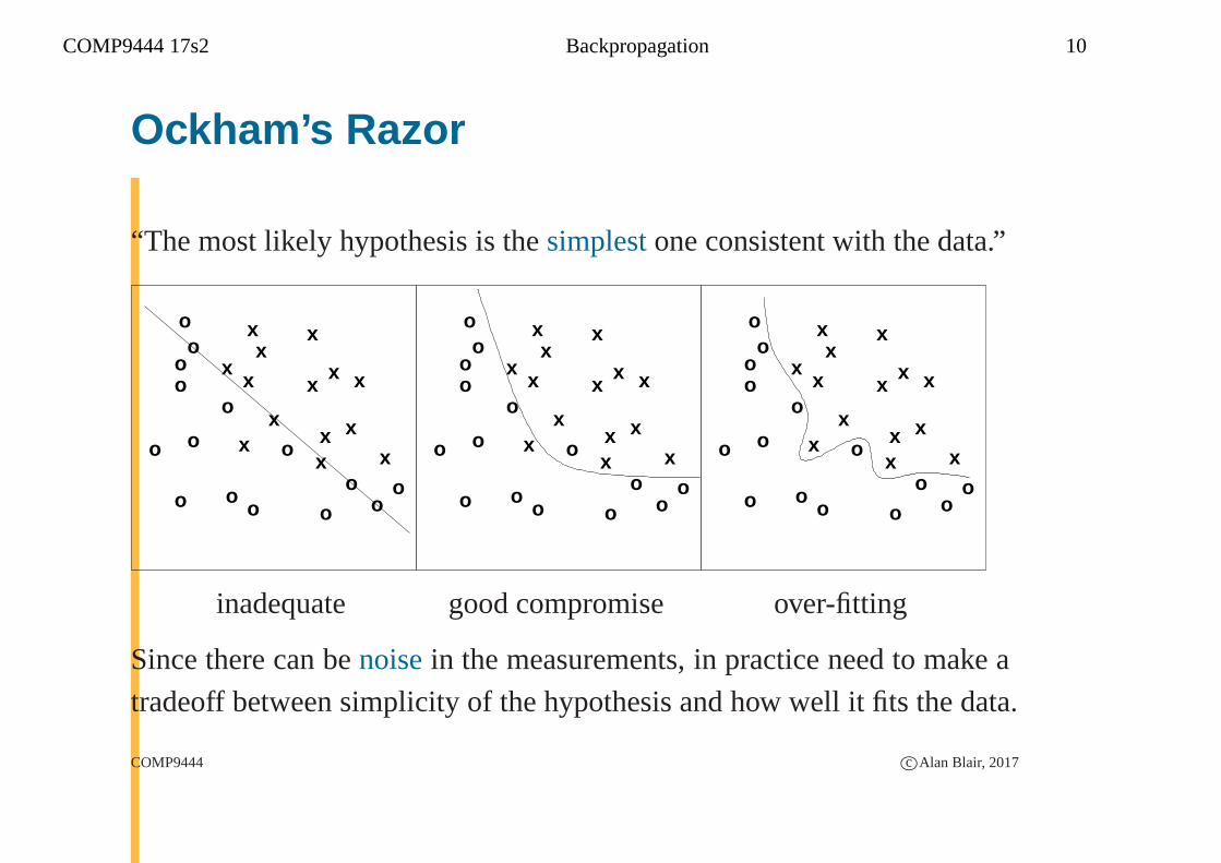
Ockham’s Razor

“The most likely hypothesis is thesimplestone consistent with the data.”

x

x

x x

x

xo

oo

o o

o

o

x

o

xx

ox

x x

x

o

x

o

o

o

o

o

x

x

x x

x

xo

oo

o o

o

o

x

o

xx

ox

x x

x

o

x

o

o

o

o

o

x

x

x x

x

xo

oo

o o

o

o

x

o

xx

ox

x x

x

o

x

o

o

o

o

o

inadequate good compromise over-fitting

Since there can benoisein the measurements, in practice need to make a

tradeoff between simplicity of the hypothesis and how well it fits the data.



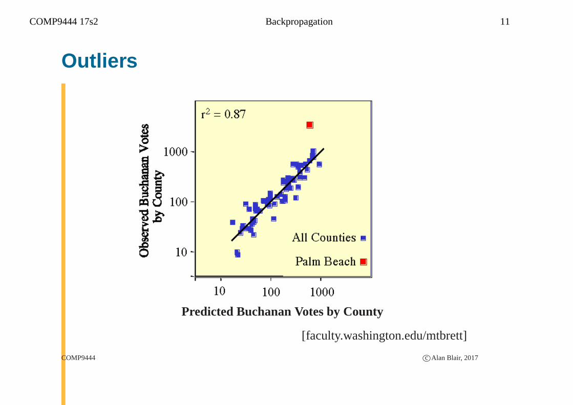
Outliers

Predicted Buchanan Votes by County

[faculty.washington.edu/mtbrett]



Butterfly Ballot



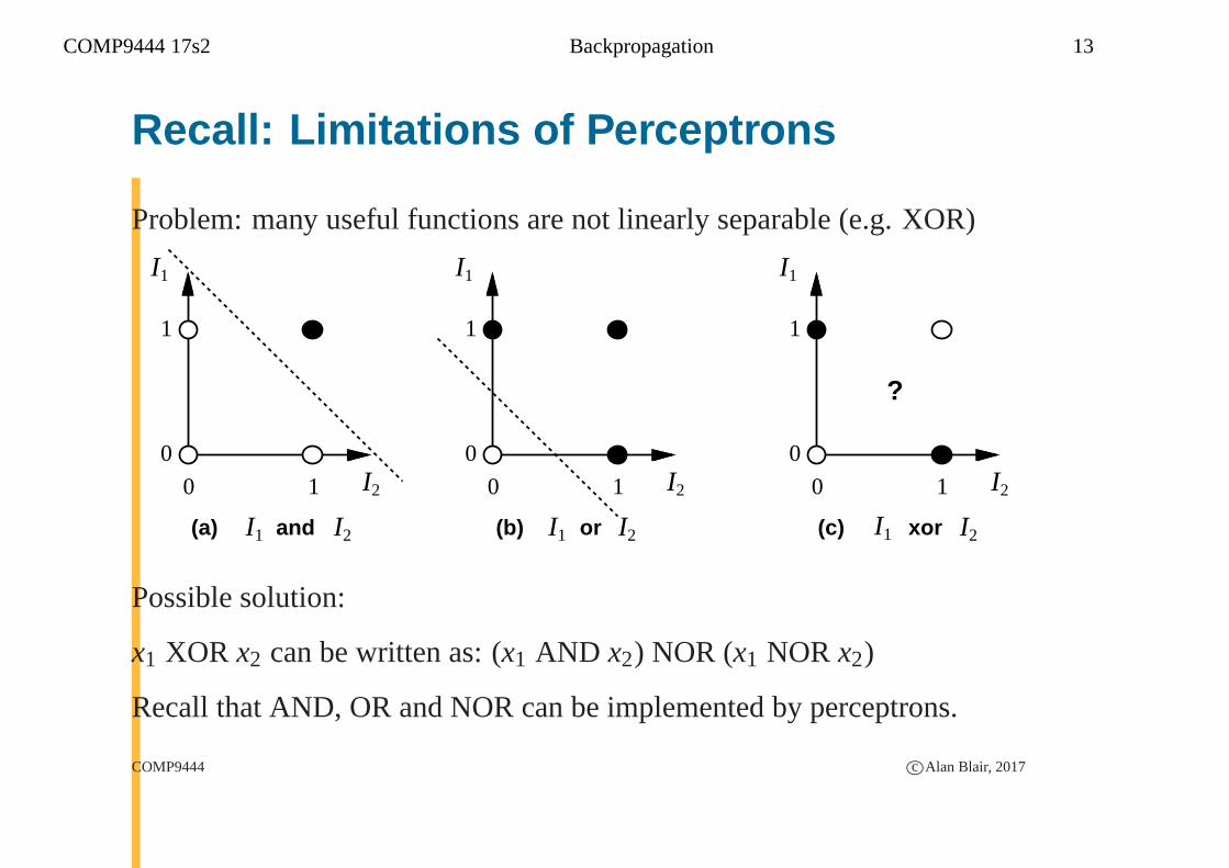
Recall: Limitations of Perceptrons

Problem: many useful functions are not linearly separable (e.g. XOR)

I 1

I 2

I 1

I 2

I 1

I 2

?

(a) (b) (c)and or xor

0 1

0

1

0

1 1

0

0 1 0 1

I 2I 1I 1 I 2I 1 I 2

Possible solution:

x1 XOR x2 can be written as: (x1 AND x2) NOR (x1 NOR x2)

Recall that AND, OR and NOR can be implemented by perceptrons.



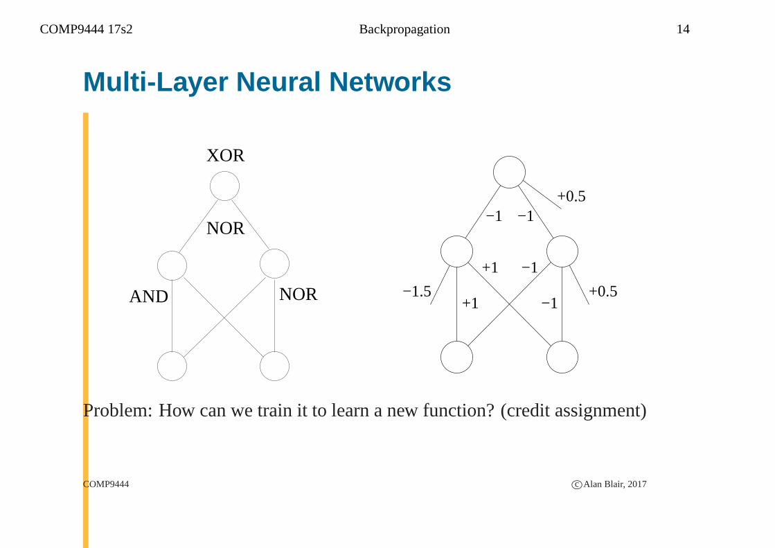
Multi-Layer Neural Networks

XOR

NOR

AND NOR

−1

+1

+1 −1−1.5

−1

−1

+0.5

+0.5

Problem: How can we train it to learn a new function? (credit assignment)



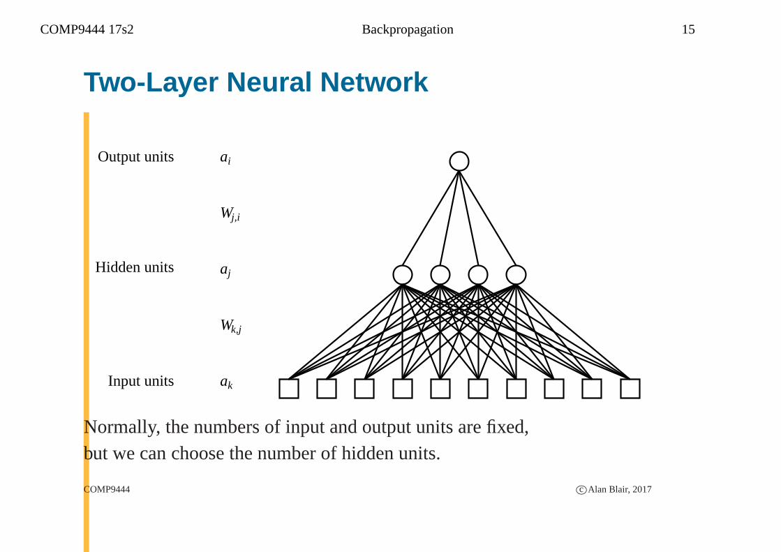
Two-Layer Neural Network

Input units

Hidden units

Output units ai

Wj,i

aj

Wk,j

ak

Normally, the numbers of input and output units are fixed,but we can choose the number of hidden units.



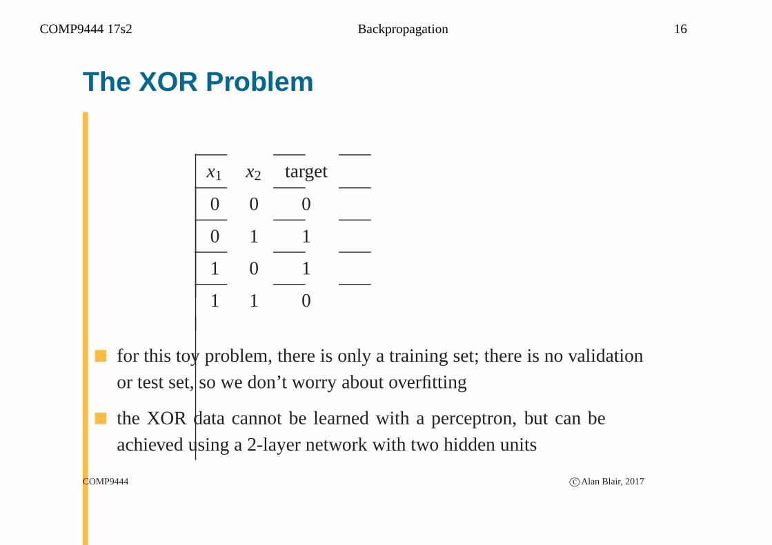
The XOR Problem

x1 x2 target

0 0 0

0 1 1

1 0 1

1 1 0

� for this toy problem, there is only a training set; there is novalidationor test set, so we don’t worry about overfitting

� the XOR data cannot be learned with a perceptron, but can beachieved using a 2-layer network with two hidden units



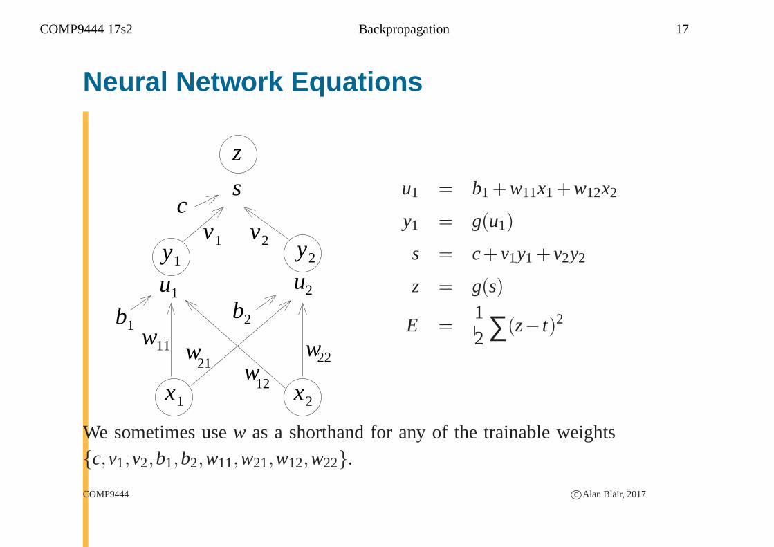
Neural Network Equations

b2

w22

b1

u1

v1 v2

z

c

u2

11w

s

w21 w

121x 2x

1y 2y

u1 = b1+w11x1+w12x2

y1 = g(u1)

s = c+ v1y1+ v2y2

z = g(s)

E =12 ∑(z− t)2

We sometimes usew as a shorthand for any of the trainable weights{c,v1,v2,b1,b2,w11,w21,w12,w22}.



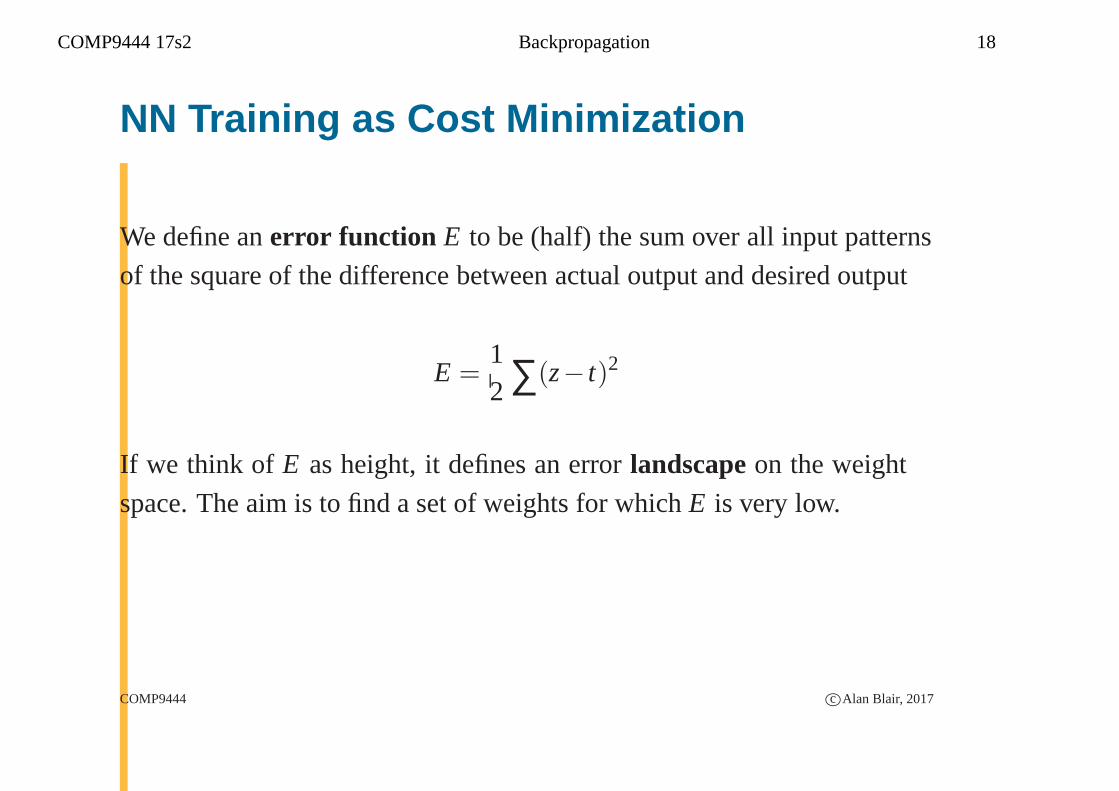
NN Training as Cost Minimization

We define anerror function E to be (half) the sum over all input patterns

of the square of the difference between actual output and desired output

E =12 ∑(z− t)2

If we think of E as height, it defines an errorlandscape on the weight

space. The aim is to find a set of weights for whichE is very low.



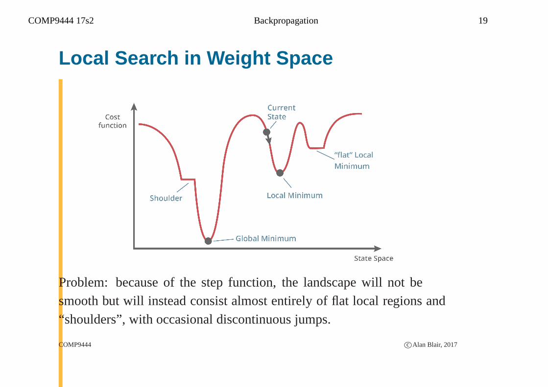
Local Search in Weight Space

Problem: because of the step function, the landscape will not besmooth but will instead consist almost entirely of flat localregions and“shoulders”, with occasional discontinuous jumps.



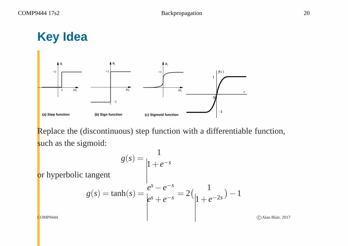
Key Idea

(a) Step function (b) Sign function

+1

ai

−1

ini

+1

ai

init

(c) Sigmoid function

+1

ai

ini

Replace the (discontinuous) step function with a differentiable function,

such as the sigmoid:

g(s) =1

1+ e−s

or hyperbolic tangent

g(s) = tanh(s) =es− e−s

es + e−s = 2( 1

1+ e−2s

)

−1



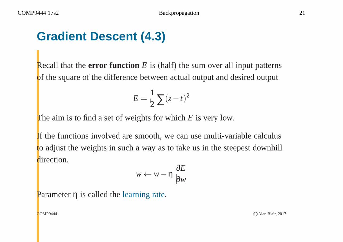
Gradient Descent (4.3)

Recall that theerror function E is (half) the sum over all input patterns

of the square of the difference between actual output and desired output

E =12 ∑(z− t)2

The aim is to find a set of weights for whichE is very low.

If the functions involved are smooth, we can use multi-variable calculus

to adjust the weights in such a way as to take us in the steepestdownhill

direction.

w← w−η∂E∂w

Parameterη is called thelearning rate.



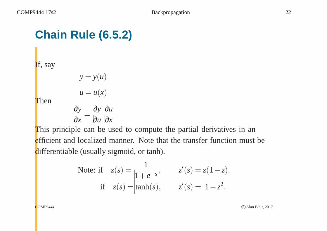
Chain Rule (6.5.2)

If, say

y = y(u)

u = u(x)Then

∂y∂x

=∂y∂u

∂u∂x

This principle can be used to compute the partial derivatives in anefficient and localized manner. Note that the transfer function must bedifferentiable (usually sigmoid, or tanh).

Note: if z(s) =1

1+ e−s , z′(s) = z(1− z).

if z(s) = tanh(s), z′(s) = 1− z2.



Forward Pass

b2

w22

b1

u1

v1 v2

z

c

u2

11w

s

w21 w

121x 2x

1y 2yu1 = b1+w11x1+w12x2

y1 = g(u1)

s = c+ v1y1+ v2y2

z = g(s)

E =12 ∑(z− t)2



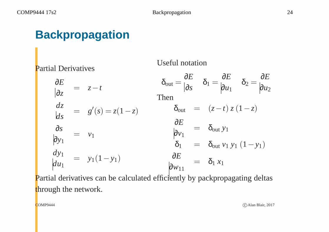
Backpropagation

Partial Derivatives

∂E∂z

= z− t

dzds

= g′(s) = z(1− z)

∂s∂y1

= v1

dy1

du1= y1(1− y1)

Useful notation

δout =∂E∂s

δ1 =∂E∂u1

δ2 =∂E∂u2

Thenδout = (z− t) z (1− z)

∂E∂v1

= δout y1

δ1 = δout v1 y1 (1− y1)

∂E∂w11

= δ1 x1

Partial derivatives can be calculated efficiently by packpropagating deltasthrough the network.



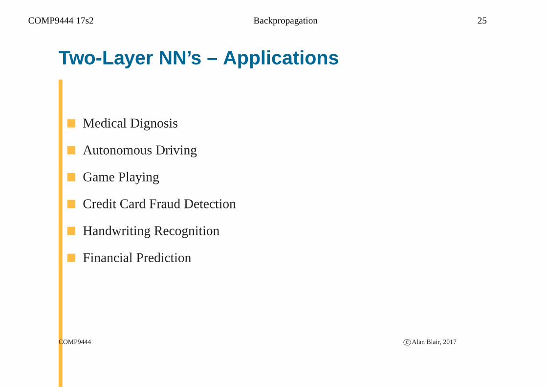
Two-Layer NN’s – Applications

� Medical Dignosis

� Autonomous Driving

� Game Playing

� Credit Card Fraud Detection

� Handwriting Recognition

� Financial Prediction



Example: Pima Indians Diabetes Dataset

Attribute mean stdv

1. Number of times pregnant 3.8 3.4

2. Plasma glucose concentration 120.9 32.0

3. Diastolic blood pressure (mm Hg) 69.1 19.4

4. Triceps skin fold thickness (mm) 20.5 16.0

5. 2-Hour serum insulin (mu U/ml) 79.8 115.2

6. Body mass index (weight in kg/(height in m)2) 32.0 7.9

7. Diabetes pedigree function 0.5 0.3

8. Age (years) 33.2 11.8

9. Class variable (0 or 1)



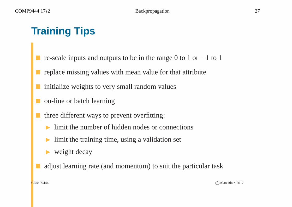
Training Tips

� re-scale inputs and outputs to be in the range 0 to 1 or−1 to 1

� replace missing values with mean value for that attribute

� initialize weights to very small random values

� on-line or batch learning

� three different ways to prevent overfitting:

◮ limit the number of hidden nodes or connections

◮ limit the training time, using a validation set

◮ weight decay

� adjust learning rate (and momentum) to suit the particular task



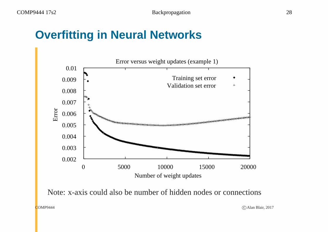
Overfitting in Neural Networks

0.002

0.003

0.004

0.005

0.006

0.007

0.008

0.009

0.01

0 5000 10000 15000 20000

Err

or

Number of weight updates

Error versus weight updates (example 1)

Training set errorValidation set error

Note: x-axis could also be number of hidden nodes or connections



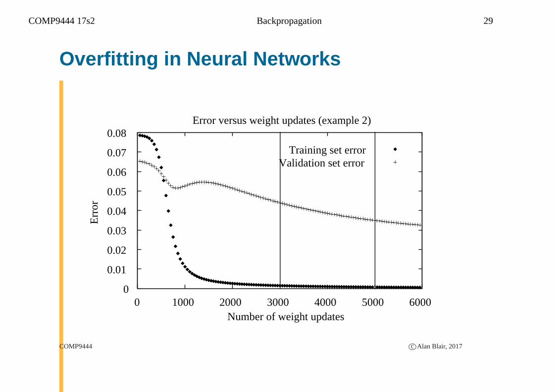
Overfitting in Neural Networks

0

0.01

0.02

0.03

0.04

0.05

0.06

0.07

0.08

0 1000 2000 3000 4000 5000 6000

Err

or

Number of weight updates

Error versus weight updates (example 2)

Training set errorValidation set error



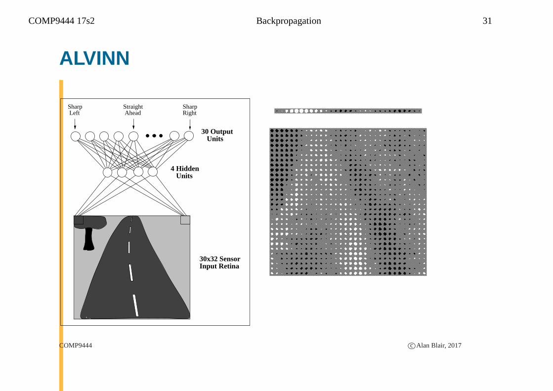
ALVINN (Pomerleau 1991, 1993)



ALVINN

Sharp Left

SharpRight

4 Hidden Units

30 Output Units

30x32 Sensor Input Retina

Straight Ahead



ALVINN

� Autonomous Land Vehicle In a Neural Network

� later version included a sonar range finder

◮ 8×32 range finder input retina

◮ 29 hidden units

◮ 45 output units

� Supervised Learning, from human actions (Behavioral Cloning)

◮ additional “transformed” training items to cover emergency

situations

� drove autonomously from coast to coast



Summary

� Neural networks are biologically inspired

� Multi-layer neural networks can learn non linearly separable functions

� Backpropagation is effective and widely used


Documents

COMP9444 Neural Networks and Deep Learning 3 ...cs9444/17s2/lect/1page/03...COMP9444 Neural Networks and Deep Learning 3. Backpropagation Textbook, Sections 4.3, 5.2, 6.5.2 COMP9444