Compact Representation of a Multi-dimensional Combustion

Compact Representation of a Multi-dimensionalCombustion Manifold Using Deep Neural

Networks

Sushrut Bhalla1[0000−0002−4398−5052], Matthew Yao1[0000−0001−6141−1477],Jean-Pierre Hickey1[0000−0002−6944−3964], and

Mark Crowley1[0000−0003−3921−4762]

University of Waterloo, Waterloo ON N2L 3G1, Canada{sushrut.bhalla,matthew.yao,j6hickey,mcrowley}@uwaterloo.ca

Abstract. The computational challenges in turbulent combustion sim-ulations stem from the physical complexities and multi-scale nature ofthe problem which make it intractable to compute scale-resolving sim-ulations. For most engineering applications, the large scale separationbetween the flame (typically sub-millimeter scale) and the character-istic turbulent flow (typically centimeter or meter scale) allows us toevoke simplifying assumptions–such as done for the flamelet model–topre-compute all the chemical reactions and map them to a low-ordermanifold. The resulting manifold is then tabulated and looked-up atrun-time. As the physical complexity of combustion simulations increases(including radiation, soot formation, pressure variations etc.) the dimen-sionality of the resulting manifold grows which impedes an efficient tab-ulation and look-up. In this paper we present a novel approach to modelthe multi-dimensional combustion manifold. We approximate the com-bustion manifold using a neural network function approximator and useit to predict the temperature and composition of the reaction. We presenta novel training procedure which is developed to generate a smooth out-put curve for temperature over the course of a reaction. We then evaluateour work against the current approach of tabulation with linear interpo-lation in combustion simulations. We also provide an ablation study ofour training procedure in the context of over-fitting in our model. Thecombustion dataset used for the modeling of combustion of H2 and O2in this work is released alongside this paper.

Keywords: Deep Learning · Combustion Manifold Modelling · Flameletmodels.

1 Introduction

The field of turbulent combustion modeling is concerned with the predictionof complex chemical reactions–and the resulting heat release–coupled with anunderlying turbulent flow field. Numerical combustion is a central design tool

2 S. Bhalla et al.

within the fields of energy production, automotive engineering (internal combus-tion engines), and aerospace engineering (rocket engines, gas turbines). The com-putational challenges in turbulent combustion simulations stem from the physicalcomplexities and multi-scale nature of the problem which make it intractable tocompute scale-resolving simulations, in spite of having a set of equations govern-ing the problem. For most engineering applications, the large scale separationbetween the flame (typically sub millimeter /microsecond scale) and the char-acteristic turbulent flow (typically centimeter or meter/minute or hour scale)allows us to evoke simplifying assumptions–such as done for the flamelet model–to pre-compute all the chemical reactions and map them to a low-order manifold;the resulting manifold can then be tabulated and looked-up at run-time. Themain benefit of the flamelet model is that is allows a decoupling of the turbulentflow field (and the inherent mixing) and the chemical reactions. The Damkohlernumber, which represents a ratio of the time scale of the chemical reactions tothe transport phenomena, is often used to bound the region of validity of theflamelet model. A simplified illustration of the flamelet model for non-premixedcombustion is shown in Figure 1. With an increasing demand on the physicalcomplexity of combustion simulations (through the inclusion of radiation, sootformation, pressure variations, wall-heat transfer etc.), the dimensionality of theresulting manifold increases and leads to the curse of dimensionality which im-pedes an efficient tabulation and look-up for engineering simulations. A centralquestion in this field is how to efficiently model high dimensional manifolds nec-essary to capture the relevant physics of the problem and relating them to thechemical composition, pressures, and other factors computed during simulations.While the underlying governing equations for the physics are available, they arehighly expensive computationally and not usable for the vast number of queriesneeded to run a combustion simulation of a realistic system. The ideal modelwould represent the well understood physical relationships in a fast, flexibleform which could use varying dimensions as needed for a particular simulationor analysis task.

In the majority of the engineering-relevant, non-premixed combustion condi-tions, there is a large scale separation between the turbulent flow and the flame.This scale separation allows us to assume that a turbulent flame is comprisedof a series of locally laminar flames, often called flamelets. This very convenientassumption is at the heart of flamelet modeling, one of the most common ap-proaches in combustion modeling. For a given pressure, injection temperature,and fuel and oxidizer composition, all possible laminar flamelets can be uniquelycharacterized by the local strain rate, which is proportional to the velocity dif-ference of the propellants in a counter-flow diffusion flame setup (see Figure 1top right). As the laminar combustion only depends on the strain rate (for agiven pressure, injector temperature and composition), all the flamelets can bepre-computed, tabulated and queried during run-time, which leads to a greatcomputational advantage for the simulation. In the classical flamelet model, thecombustion in any part of the computational domain can be uniquely defined bythe local mixture fraction, Z (a conserved quantity which varies between 0 for

Compact Representation of a Combustion Manifold 3

Fig. 1: A turbulent non-premixed flame is illustrated (left). The corrugated turbulentflame is assumed to be made up of locally laminar flames (as illustrated in the topright). The laminar flame (top right) can be computed, a priori, for all strain ratesand tabulated for lookup at run-time. The tabulation is often done with respect to theknown/transported variables from the simulation such as mixture fraction, Z, progress-variable C, variance of mixture fraction Z′′, pressure, P (bottom right).

pure oxidizer and 1 for pure fuel), strain rate, χ (time scale ratio between thechemical reactions and the flow), and the mixture fraction variance, Z ′′ (whichaccounts for the turbulent mixing). More recent variations of the flamelet modelhave replaced the strain rate by a non-conservative progress variable, C. Thislatest model is called the Flamelet-Progress Variable Approach (FPVA). Thereader interested in a more comprehensive overview of these combustion model-ing paradigms is invited to consult [22].

In recent years, deep learning has been used to achieve state of the art resultsin image classification [5, 26], policy learning [18, 12] and natural language pro-cessing [25]. Deep learning has the ability to learn compact representations andcan naturally handle interpolation of points which are not part of the trainingdata. For the combustion modeling problem, our hypothesis is that deep learn-ing can be used to learn a model of the higher dimension combustion manifoldwhich can be used for simulation. In this paper we present an architecture totest this hypothesis and the techniques, including novel ones, we used to train adiscriminative model for combustion. We show that we can reduce the combus-tion simulation running time and memory requirements compared to the currenttabular methods. To examine the relative impact of each model component, wepresent an ablation study of our regularization methods and training techniques.We also propose an improved over-sampling procedure and a loss function whichforces the model to focus on more difficult data points during training. Signifi-cant improvements in modeling for the combustion modeling problem could leadto a revolution in the ability to simulate complex combustion reactions and more

4 S. Bhalla et al.

efficiently design better engines and power systems. This paper sets the ground-work for such a change by showing how to use deep learning to free modelersfrom the limits of tabular representations.

2 Related Work

Over the years the classical flamelet methodologies have been extended to tackleincreasingly complex reactive flow problems. For example, the slow time-scaleof NOx formation has motivated the use of unsteady flamelet [16] and the needto account for radiative heat loss effects due to the sensitivity to temperatureof the NO formation has resulted in an FPV framework that includes an addi-tional enthalpy term [7]. Similarly, the strong heat loss at the combustor wallshas motivated a wall heat loss model [15, 24] which also includes an additionalenthalpy term. Many combustion processes, such as liquid rocket combustion,are undertaken under variable pressure conditions which has been integratedinto the flamelet framework [17]. Other extensions includes the consideration ofmulti-fuel systems [3]–which demand the use of two separate mixture fractions– or the inclusion of combustion chemistry that is highly sensitive to moleculardiffusion (primarily in partially premixed settings) resulting in the introductionof multidimensional flamelet-generated manifolds (MFM) [20].

There is a growing demand to accurately represent the combustion processin more complex combustion scenarios such as those above. However, this re-quires a higher-dimensional manifold than the widely used FPVA method whichcommonly utilizes a three-dimensional tabulation of all the variables of interest,φ(Z, ˜Z ′′2, c). Not only does the tabulated data occupy a larger portion of theavailable memory, the searching and retrieval of the pre-tabulated data becomesincreasingly expensive in a higher-dimensional space. For example, assuming astandard flamelet table discretization of (nZ, nZvar, nC) = (200, 100, 50) withsay 15 tabulated variables, we obtain a pre-computed combustion table of 120Mb. The addition of a variable such as enthalpy with a very coarse discretizationof 20 points, brings the size of the table to 2.4 Gb. Recent consideration of ahigh-dimensional flamelet generated manifold for stratified-swirled flames withwall heat loss requires a 5D manifold which would be even larger [2]. This couldonly be achieved by using a very coarse discretization of the flamelet manifold(e.g. only 10 points are used to account for the variance of mixture fraction).One approach to address the large tabulative size has been proposed by us-ing polynomial basis functions [27]; other approaches have looked at the use ofBezier patches [28]. These approaches provide adequate ways to reduce the tab-ulation size, retrieval time and improve accuracy, but face the inevitable curseof dimensionality. Other approaches seek to use principle component analysisto identify the optimal progress variable for the definition of a low-dimensionalmanifold [19]. Even if those approaches prove effective, inevitably many multi-physics systems will require a higher-dimensional space to adequately capturethe relevant processes.


There has been some previous work on using machine learning for combustionmanifold modeling. In 2009, a thorough experimental comparison was carried outby Ihme et al. [8] using a simple Multi-Layer Perceptron (MLP) for learning amapping function to replace the tabular lookup method and thus speed up com-bustion simulation calculations. They showed that a neural network approachcould be more generalizable but they found it had much worse accuracy thanthe tabular approach. This led to the method not being adopted for combustionsimulator evaluations by the community. The approach in [8] was limited to asimple range of MLP variations and focused on the optimization of the networkstructure relative to a particular metric. They also did not have the benefit ofmodern deep neural network training techniques or regularization methods andused the classical approach of sigmoid activation functions rather than rectifiedlinear units. In this work we focus on finding an optimal deep neural networktraining strategy which can achieve results approximately close to the true datacurves. We show that our loss function and over sampling methods can achievebetter accuracy than [8]. We also demonstrate our approach provides an accel-eration over tabular methods for realistic combustion simulator evaluations byleveraging a CUDA enabled GPU. We also implement trained models for thespecies composition, temperature, source term and heat release.

Recent work [11] has focused on predicting the subgrid scale wrinkling ofa flame by using a convolutional neural network. The work focuses on trainingan autoencoder with a U-Net network structure, which uses the current Di-rect Numerical Simulation (DNS) snapshot to predict the next DNS snapshot.The training data is a collection of 2 DNS of different flames; a third DNS isused for testing. This is a very simplified model to account for combustion anddoesn’t make any flamelet-based assumptions. Using a temporally dependentdata structure for training limits the work in [11] and it cannot be easily ex-tended to instantaneous combustion evaluations. Their model also requires theflame to be extrapolated to a certain length for the CNN model to be effective,as the autoencoder model they use would fail at the boundary conditions of theflame. In contrast, our model is built with the understanding that there can bemultiple flames being simulated at a given instance and they could be running atdifferent resolutions. Resolution in combustion simulations represents the factorby which the flamelet has been discretized based on the precision and accuracyrequired by the researcher. Thus, our model is built using fully connected layerswhich map the pressure, mixture fraction and progress variable to the speciescomposition, temperature, source term and heat release.

3 Modeling Methods for High Dimensional Data

In this section we present the techniques we used to train our deep neural net-work model to predict the composition of the species (H, O2, O, OH, H2,H2O, HO2, H2O2), temperature (T ), source term (W ) and heat release (HR)of any flamelet given the pressure (P ), progress variable (C) and mixture frac-tion (Z). The training data consists of flamelets for pressure values in the set

6 S. Bhalla et al.

(1, 2, 5, 10, 20, 30, 35, 40, 50)bar and the associated progress variable (C) and mix-ture fraction (Z). We reserve flames at pressure values (15, 25, 33, 42)bar for test-ing purposes. The validation data set is generated by sampling sections of theflames in the training data set. The data was generated using FlameMaster, a 1Dsolver for the solution of the laminar, diffusion flamelet equations. The flameletswere generated at varying strain rates, from equilibrium combustion to nearlythe quenched solution at varying base pressure levels. For all flamelets, the in-flow temperature of the fuel and oxidizer remain constant. At each condition,the flamelets are solved with 1001 grid points with local mesh adaptation.

3.1 Neural Network Design

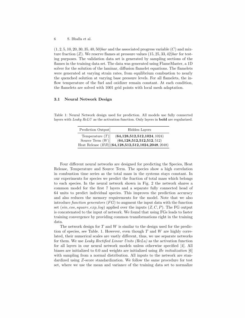
Table 1: Neural Network design used for prediction. All models use fully connectedlayers with Leaky ReLU as the activation function. Only layers in bold are regularized.

Prediction Output Hidden Layers

Temperature (T ) (64,128,512,512,1024, 1024)Source Term (W ) (64,128,512,512,512, 512)

Heat Release (HR) (64,128,512,512,1024,2048, 2048)

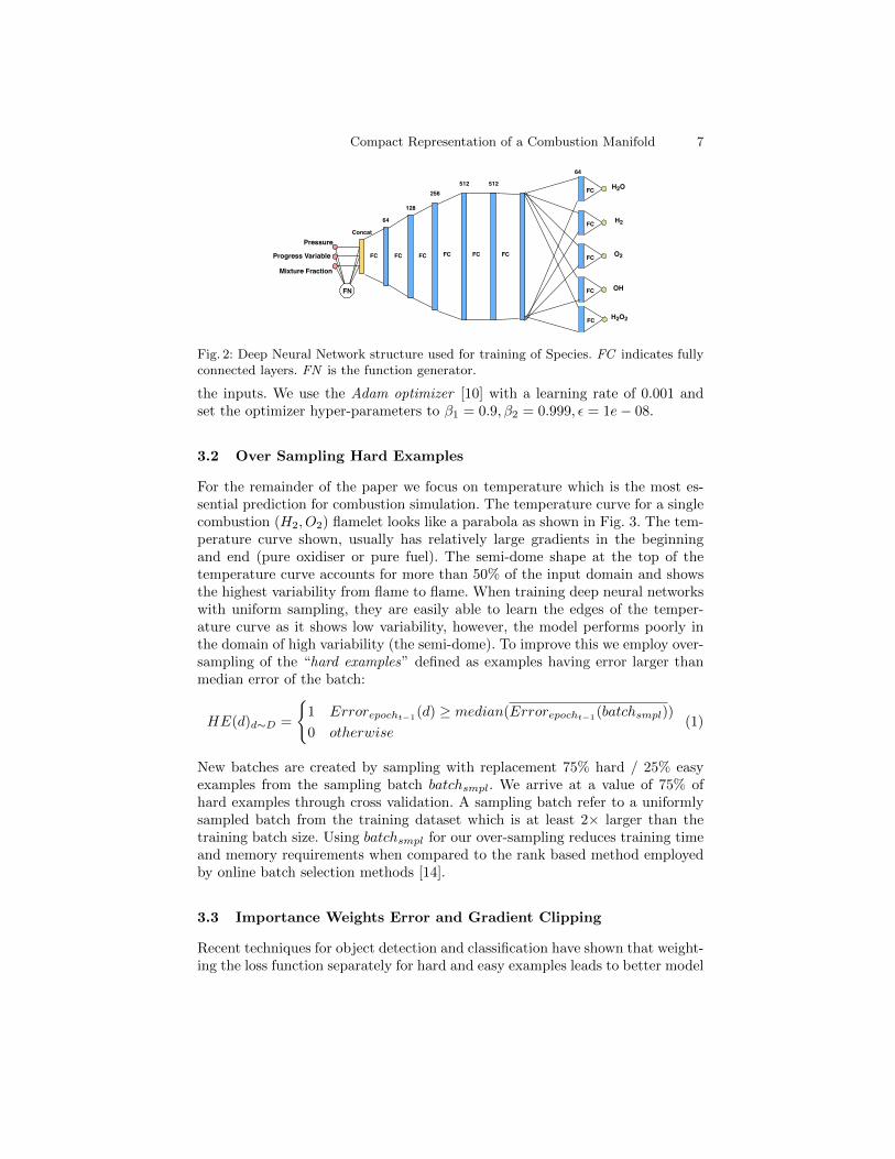
Four different neural networks are designed for predicting the Species, HeatRelease, Temperature and Source Term. The species show a high correlationin combustion time series as the total mass in the systems stays constant. Inour experiments for species we predict the fraction of total mass which belongsto each species. In the neural network shown in Fig. 2 the network shares acommon model for the first 7 layers and a separate fully connected head of64 units to predict individual species. This improves the prediction accuracyand also reduces the memory requirements for the model. Note that we alsointroduce function generators (FG) to augment the input data with the functionset (sin, cos, square, exp, log) applied over the inputs (Z,C, P ). The FG outputis concatenated to the input of network. We found that using FGs leads to fastertraining convergence by providing common transformations right in the trainingdata.

The network design for T and W is similar to the design used for the predic-tion of species, see Table. 1. However, even though T and W are highly corre-lated, their numerical scales are vastly different, thus, we use separate networksfor them. We use Leaky Rectified Linear Units (ReLu) as the activation functionfor all layers in our neural network models unless otherwise specified [4]. Allbiases are initialized to 0.0 and weights are initialized using He initialization [6]with sampling from a normal distribution. All inputs to the network are stan-dardized using Z-score standardization. We follow the same procedure for testset, where we use the mean and variance of the training data set to normalize


FN

FCFCFCFCFC FC

Mixture Fraction

64

256

128

512512

64

FC H2O

ConcatPressure

Progress Variable

FC H2

FC O2

FC OH

FC H2O2

Fig. 2: Deep Neural Network structure used for training of Species. FC indicates fullyconnected layers. FN is the function generator.

the inputs. We use the Adam optimizer [10] with a learning rate of 0.001 andset the optimizer hyper-parameters to β1 = 0.9, β2 = 0.999, ε = 1e− 08.

3.2 Over Sampling Hard Examples

For the remainder of the paper we focus on temperature which is the most es-sential prediction for combustion simulation. The temperature curve for a singlecombustion (H2, O2) flamelet looks like a parabola as shown in Fig. 3. The tem-perature curve shown, usually has relatively large gradients in the beginningand end (pure oxidiser or pure fuel). The semi-dome shape at the top of thetemperature curve accounts for more than 50% of the input domain and showsthe highest variability from flame to flame. When training deep neural networkswith uniform sampling, they are easily able to learn the edges of the temper-ature curve as it shows low variability, however, the model performs poorly inthe domain of high variability (the semi-dome). To improve this we employ over-sampling of the “hard examples” defined as examples having error larger thanmedian error of the batch:

HE(d)d∼D =

{1 Errorepocht−1(d) ≥ median(Errorepocht−1

(batchsmpl))

0 otherwise(1)

New batches are created by sampling with replacement 75% hard / 25% easyexamples from the sampling batch batchsmpl. We arrive at a value of 75% ofhard examples through cross validation. A sampling batch refer to a uniformlysampled batch from the training dataset which is at least 2× larger than thetraining batch size. Using batchsmpl for our over-sampling reduces training timeand memory requirements when compared to the rank based method employedby online batch selection methods [14].

3.3 Importance Weights Error and Gradient Clipping

Recent techniques for object detection and classification have shown that weight-ing the loss function separately for hard and easy examples leads to better model

8 S. Bhalla et al.

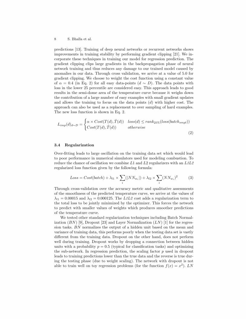
predictions [13]. Training of deep neural networks or recurrent networks showsimprovements in training stability by performing gradient clipping [21]. We in-corporate these techniques in training our model for regression prediction. Thegradient clipping clips large gradients in the backpropagation phase of neuralnetwork training and thus reduces any damage to our trained model caused byanomalies in our data. Through cross validation, we arrive at a value of 5.0 forgradient clipping. We choose to weight the cost function using a constant valueof α = 0.4 (in Eq. 2) for all easy data-points (d ∼ D). The data points withloss in the lower 25 percentile are considered easy. This approach leads to goodresults in the semi-dome area of the temperature curve because it weighs downthe contribution of a large number of easy examples with small gradient updatesand allows the training to focus on the data points (d) with higher cost. Theapproach can also be used as a replacement to over sampling of hard examples.The new loss function is shown in Eq. 2.

Limp(d)d∼D =

{α× Cost(T (d), T (d)) loss(d) ≤ rank25%(loss(batchsmpl))

Cost(T (d), T (d)) otherwise

(2)

3.4 Regularization

Over-fitting leads to large oscillation on the training data set which would leadto poor performance in numerical simulators used for modeling combustion. Toreduce the chance of oscillation we combine L1 and L2 regularizers with an L1L2regularized loss function given by the following formula:

Loss = Cost(batch) + λl1 ×∑i

(|NNwi |) + λl2 ×∑i

(NNwi)2 (3)

Through cross-validation over the accuracy metric and qualitative assessmentsof the smoothness of the predicted temperature curve, we arrive at the values ofλl1 = 0.00015 and λl2 = 0.000125. The L1L2 cost adds a regularization term tothe total loss to be jointly minimized by the optimizer. This forces the networkto predict with smaller values of weights which produces smoother predictionsof the temperature curve.

We tested other standard regularization techniques including Batch Normal-ization (BN) [9], Dropout [23] and Layer Normalization (LN) [1] for the regres-sion tasks. BN normalizes the output of a hidden unit based on the mean andvariance of training data, this performs poorly when the testing data set is vastlydifferent from the training data. Dropout on the other hand, does not performwell during training. Dropout works by dropping a connection between hiddenunits with a probability p = 0.5 (typical for classification tasks) and optimizingthe sub-network. In regression prediction, the scaling factor p used in dropoutleads to training predictions lower than the true data and the reverse is true dur-ing the testing phase (due to weight scaling). The network with dropout is notable to train well on toy regression problems (for the function f(x) = x2). LN


normalizes the input features of the hidden layers on a per data point basis andthus doesn’t exhibit the problems from batch normalization. LN seems to be abetter fit than batch normalization and dropout for regression tasks, however aswe show in the experiments section, the performance with L1L2 regularizationis better.

3.5 Ensemble Model

Many machine learning tasks have shown improved results by using an ensembleof models. In regression, ensembles of models would be highly beneficial as itwould reduce the amount of regularization required per model and the accuracycould be improved with careful selection of a set of prediction models. We de-sign an averaging ensemble of trained models. We train five deep neural networkmodels for prediction of the temperature curve. The ensemble model also helpsin improving the accuracy of the model. We compute the final prediction by av-eraging the four best (in terms of deviation from the mean prediction) individualmodels. This allows us to ignore results from models which didn’t perform wellon certain data-points and pick the best of all trained models.

4 Results and Discussions

4.1 Quantitative Analysis

Table 2 shows the accuracy and the loss for each prediction variable. A predictionis considered accurate if the model prediction (T (d)) is within a standard errorrange ET , as shown in the formula below for the temperature model:

accuracyd∼D =

{1 T (d) ∈ {T (d)− ET , T (d) + ET }0 otherwise

(4)

The value of EO (where O ∈ {T,W,HR, Species}) is computed based onthe resolution of the combustion simulator and an expert’s opinion. The valueof 0.005× range is used based on the discretization error in typical combustionsimulations arising from tabulation method. We detail the values of EO foreach output label in the Table 2. Accuracy is used for model comparison sinceusing the resulting MSE could be misleading. That’s because the model could beperforming well on easy examples (head and tail of T curves) and poorly on thehard examples (mostly in the semi-dome part of the curve). This would resultin a lower loss value but poor accuracy for simulator evaluation purposes.

We focus on the predictions of T and W for our work as their performanceis vital for our model to be useful for the combustion community. The meanerror results in Table. 2 are computed using the formula ME = 1

N

∑N1 (|y− y|).

For temperature, we see a mean error of 82.44 which is the deviation from thetabulated data on test data set. We show using our simulation tests that thiserror is sustainable and can be used in combustion simulators. The accuracy of

10 S. Bhalla et al.

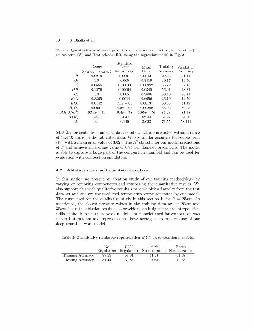
Table 2: Quantitative analysis of predictions of species composition, temperature (T),source term (W) and Heat release (HR) using the regression model in Fig. 2

Range

(OMAX −OMIN )

StandardError

Range (EO)MeanError

TrainingAccuracy

ValidationAccuracy

H 0.0219 0.0001 0.00431 29.23 21.44O2 1.0 0.005 0.3419 20.17 12.56O 0.0665 0.00033 0.00892 55.79 37.43

OH 0.1279 0.00064 0.0345 56.91 43.34H2 1.0 0.005 0.2606 38.40 25.41

H2O 0.8865 0.0044 0.6056 26.19 14.59HO2 0.0142 7.1e− 05 0.00137 60.36 41.42H2O2 0.0091 4.5e− 05 0.00259 55.92 36.05

HR(J/m3) 93.4e+ 81 6.4e+ 78 1.05e+ 76 81.23 81.18T (K) 3295 34.47 82.44 61.97 54.60

W 30 0.149 3.023 71.55 58.144

54.60% represents the number of data points which are predicted within a rangeof 34.47K range of the tabulated data. We see similar accuracy for source term(W ) with a mean error value of 3.023. The R2 statistic for our model predictionsof T and achieve an average value of 0.94 per flamelet predictions. The modelis able to capture a large part of the combustion manifold and can be used forevaluation with combustion simulators.

4.2 Ablation study and qualitative analysis

In this section we present an ablation study of our training methodology byvarying or removing components and comparing the quantitative results. Wealso support this with qualitative results where we pick a flamelet from the testdata set and analyze the predicted temperature curve generated by our model.The curve used for the qualitative study in this section is for P = 25bar. Asmentioned, the closest pressure values in the training data are at 20bar and30bar. Thus the ablation results also provide us an insight into the interpolationskills of the deep neural network model. The flamelet used for comparison wasselected at random and represents an above average performance case of ourdeep neural network model.

Table 3: Quantitative results for regularization of NN on combustion manifold.

NoRegularizer

L1L2Regularizer

LayerNormalization

BatchNormalization

Training Accuracy 87.59 59.01 44.53 61.68Testing Accuracy 31.44 39.83 23.63 12.28


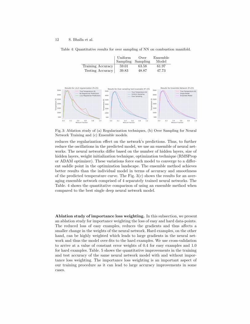
Ablation study of regularization techniques. Fig. 3(a) shows the qual-itative results for training the neural network with L1L2 regularization andwithout any regularization. The L1L2 regularization forces the weights of theneural network to be closer to 0. This affects the temperature curve generatedby our regularized model as seen in Fig. 3(a). The curve shows very little oscil-lations which is necessary condition for our model to be used in real combustionsimulators. Due to the restriction on the weights of the neural network, ourmodel suffers in terms of performance as we get a temperature curve distantfrom the true data curve. Table. 3 summarizes the performance of using differ-ent regularization techniques. The value of λL1, λL2 is set to 0.00015, 0.000125respectively. We see that L1L2 regularization performs the best on test dataset. We thus use L1L2 for all the experiments. BN is also able to train well onthe training data set, but performs poorly when the distribution of the data ischanged during testing. BN was also not able to scale to larger batch sizes andthus suffered in performance when compared to other methods. LN alleviatesthe dependence on the training data and normalizes each layer’s input features.This results in better performance, and the results of LN are more predictablethan batch normalization.

Ablation study of over sampling. Next we examine the incremental effect ofusing over sampling of hard examples from the data set based on the mean squareerror for each data-point in the previous training epoch. Fig. 3(b) shows the com-parison of the predicted temperature curves for using over-sampling comparedto basic uniform sampling. Both training methods use L1L2 regularization withthe same hyper-parameters as last subsection. The results clearly show that oversampling is able to better approximate the temperature curve. The over samplingof hard examples allows the network to improve its predictions on semi-domestructure near the top of the temperature curve. The network is able to approxi-mate the beginning and end of the temperature curve as seen with a naive neuralnetwork model in Fig. 3(b). The plot shows the temperature (same as previoussubsection) curve for a flame at pressure value of 25bar over the mixture frac-tion. The mixture fraction denotes the progress of the 3−D combustion flame.Table. 4 shows the quantitative improvements in the prediction accuracy of thetemperature curves for over-sampling with the same neural network structureand training hyper-parameters used for uniform sampling case. The results showa direct improvement in the qualitative curve structure and the accuracy metric.The fraction of hard examples per batch was set to 0.75 through cross validation.

Ablation study of ensemble model. Next we present an ablation studyof the ensemble model used in our work. The Fig. 3(c) shows the comparisonof predicted temperature curves for the ensemble method against the best sin-gle model temperature curve achieved using over sampling. While regularizationreduces the oscillation in the neural network predictions, the over-sampling tech-nique forces the network to shift its weights to focus on the hard examples. This

12 S. Bhalla et al.

Table 4: Quantitative results for over sampling of NN on combustion manifold.

UniformSampling

OverSampling

EnsembleModel

Training Accuracy 59.01 63.58 61.97Testing Accuracy 39.83 48.87 47.73

0.0 0.2 0.4 0.6 0.8 1.0Mixture Fraction

500

1000

1500

2000

2500

3000

3500

Tem

pera

ture

(K)

Results for L1L2 regularization (P=25)True Temperature (K)No Regularizer PredictionsL1L2 Regularizer Predictions


500

1000

1500

2000

2500

3000

3500

Tem

pera

ture

(K)

Results for Over sampling hard examples (P=25)True Temperature (K)Uniform SamplingOver Sampling


500

1000

1500

2000

2500

3000

3500

Tem

pera

ture

(K)

Results for Ensemble Network (P=25)True Temperature (K)Single ModelEnsemble Model

Fig. 3: Ablation study of (a) Regularization techniques, (b) Over Sampling for NeuralNetwork Training and (c) Ensemble models.

reduces the regularization effect on the network’s predictions. Thus, to furtherreduce the oscillations in the predicted model, we use an ensemble of neural net-works. The neural networks differ based on the number of hidden layers, size ofhidden layers, weight initialization technique, optimization technique (RMSPropor ADAM optimizer). These variations force each model to converge to a differ-ent saddle point in the optimization landscape. The ensemble method achievesbetter results than the individual model in terms of accuracy and smoothnessof the predicted temperature curve. The Fig. 3(c) shows the results for an aver-aging ensemble network comprised of 4 separately trained neural networks. TheTable. 4 shows the quantitative comparison of using an ensemble method whencompared to the best single deep neural network model.

Ablation study of importance loss weighting. In this subsection, we presentan ablation study for importance weighting the loss of easy and hard data-points.The reduced loss of easy examples, reduces the gradients and thus affects asmaller change in the weights of the neural network. Hard examples, on the otherhand, can be highly weighted which leads to large gradients in the neural net-work and thus the model over-fits to the hard examples. We use cross-validationto arrive at a value of constant error weights of 0.4 for easy examples and 1.0for hard examples. Table. 5 shows the quantitative improvements in the trainingand test accuracy of the same neural network model with and without impor-tance loss weighting. The importance loss weighting is an important aspect ofour training procedure as it can lead to large accuracy improvements in somecases.


Table 5: Comparison of impact on accuracy for differing levels of α in Eq. 2 for hardand easy data. Uses the Mean Square Error cost function.

H O2 O OH H2 H2O HO2 H2O2 T (K) W

α = 1.0 29.23 18.05 55.79 45.58 38.40 60.56 60.36 55.92 61.97α = 0.4 46.57 43.6 62.3 51.6 38.51 85.76 62.14 67.41 63.64


500

1000

1500

2000

2500

3000

3500

Temp

erat

ure (

K)

Results for Ensemble Network (P=33)Actual T (K)Predictions for P=33


500

1000

1500

2000

2500

3000

3500

Temp

erat

ure (

K)

Results for Ensemble Network (P=42)Actual T (K)Predictions for P=42

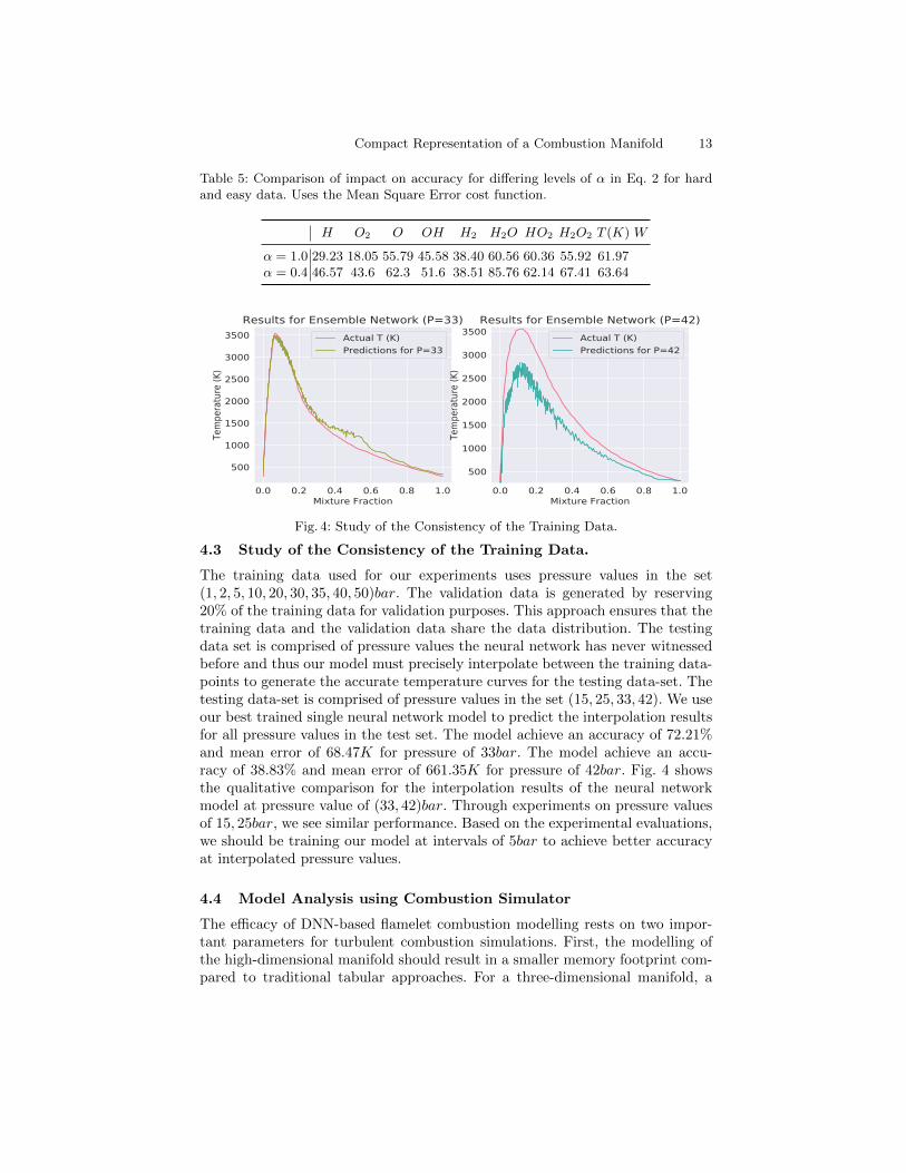
Fig. 4: Study of the Consistency of the Training Data.

4.3 Study of the Consistency of the Training Data.

The training data used for our experiments uses pressure values in the set(1, 2, 5, 10, 20, 30, 35, 40, 50)bar. The validation data is generated by reserving20% of the training data for validation purposes. This approach ensures that thetraining data and the validation data share the data distribution. The testingdata set is comprised of pressure values the neural network has never witnessedbefore and thus our model must precisely interpolate between the training data-points to generate the accurate temperature curves for the testing data-set. Thetesting data-set is comprised of pressure values in the set (15, 25, 33, 42). We useour best trained single neural network model to predict the interpolation resultsfor all pressure values in the test set. The model achieve an accuracy of 72.21%and mean error of 68.47K for pressure of 33bar. The model achieve an accu-racy of 38.83% and mean error of 661.35K for pressure of 42bar. Fig. 4 showsthe qualitative comparison for the interpolation results of the neural networkmodel at pressure value of (33, 42)bar. Through experiments on pressure valuesof 15, 25bar, we see similar performance. Based on the experimental evaluations,we should be training our model at intervals of 5bar to achieve better accuracyat interpolated pressure values.

4.4 Model Analysis using Combustion Simulator

The efficacy of DNN-based flamelet combustion modelling rests on two impor-tant parameters for turbulent combustion simulations. First, the modelling ofthe high-dimensional manifold should result in a smaller memory footprint com-pared to traditional tabular approaches. For a three-dimensional manifold, a

14 S. Bhalla et al.

Table 6: Memory Requirements and Inference Time Analysis

Tabulation Method Deep Neural Networks

Parallel Inference Time (in ms) 1.2× 105 ms 13.92Serial Inference Time (in s) 10.997 ms 55.27

Memory Requirements 184.64 MB 24.158 MB

compact representation takes up about 8 times less memory compared to anadequately resolved table. With increasing dimensionality of the combustionmanifold (inclusion of wall heating, NOx computations etc.) the impact on theDNN model is modest whereas we typically expect a two decade increase in thetable size per additional dimension. Second, the query time should be quick forN−dimensional interpolations for simulator evaluations as the size of data anddimensionality increases. Table. 6 shows the query time for 50, 000 data pointsperformed in serial and batch fashions. The simulator evaluations can be easilyparallelized to take advantage of the batched inference time.

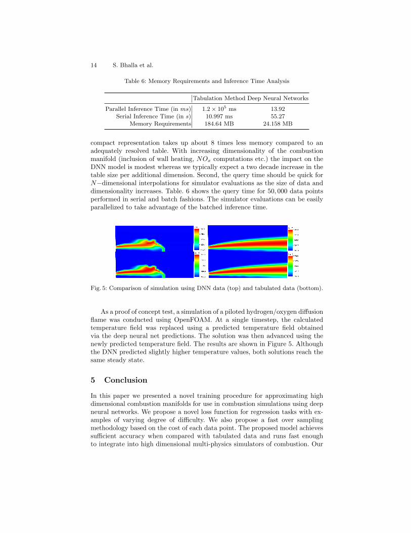
Fig. 5: Comparison of simulation using DNN data (top) and tabulated data (bottom).

As a proof of concept test, a simulation of a piloted hydrogen/oxygen diffusionflame was conducted using OpenFOAM. At a single timestep, the calculatedtemperature field was replaced using a predicted temperature field obtainedvia the deep neural net predictions. The solution was then advanced using thenewly predicted temperature field. The results are shown in Figure 5. Althoughthe DNN predicted slightly higher temperature values, both solutions reach thesame steady state.

5 Conclusion

In this paper we presented a novel training procedure for approximating highdimensional combustion manifolds for use in combustion simulations using deepneural networks. We propose a novel loss function for regression tasks with ex-amples of varying degree of difficulty. We also propose a fast over samplingmethodology based on the cost of each data point. The proposed model achievessufficient accuracy when compared with tabulated data and runs fast enoughto integrate into high dimensional multi-physics simulators of combustion. Our


model allows for cheap computation of very complex physics, compared to thetraditional tabulation methods which can not scale to high dimensions. We planto extend this work to focus on dimensionality reduction to understand core as-pects of the combustion manifold. Our prediction model for HR does not performadequately as the output range of HR is large (1081). The drawering techniquediscussed in [29] can be used to reduce the complexity of learning the range ofHR.

References

1. Ba, J.L., Kiros, J.R., Hinton, G.E.: Layer normalization. arXiv preprintarXiv:1607.06450 (2016)

2. Donini, A., M. Bastiaans, R.J., van Oijen, J.A., H. de Goey, L.P.: A 5-D Implemen-tation of FGM for the Large Eddy Simulation of a Stratified Swirled Flame withHeat Loss in a Gas Turbine Combustor, vol. 98. Flow, Turbulence and Combustion(2017)

3. Felsch, C., Gauding, M., Hasse, C., Vogel, S., Peters, N.: An extended flameletmodel for multiple injections in di Diesel engines. Proceedings of the CombustionInstitute 32 II, 2775–2783 (2009)

4. Glorot, X., Bordes, A., Bengio, Y.: Deep sparse rectifier neural networks. In: Pro-ceedings of the fourteenth international conference on artificial intelligence andstatistics. pp. 315–323 (2011)

5. Graham, B.: Fractional max-pooling. arXiv preprint arXiv:1412.6071 (2014)

6. He, K., Zhang, X., Ren, S., Sun, J.: Deep residual learning for image recognition. In:Proceedings of the IEEE conference on computer vision and pattern recognition.pp. 770–778 (2016)

7. Ihme, M., Pitsch, H.: Modeling of radiation and nitric oxide formation in turbu-lent nonpremixed flames using a flamelet/progress variable formulation. Physics ofFluids 20(5) (2008)

8. Ihme, M., Schmitt, C., Pitsch, H.: Optimal artificial neural networks and tabulationmethods for chemistry representation in les of a bluff-body swirl-stabilized flame.Proceedings of the Combustion Institute 32 I(1), 1527–1535 (2009),

9. Ioffe, S., Szegedy, C.: Batch normalization: Accelerating deep network training byreducing internal covariate shift. arXiv preprint arXiv:1502.03167 (2015)

10. Kingma, D.P., Ba, J.: Adam: A method for stochastic optimization. arXiv preprintarXiv:1412.6980 (2014)

11. Lapeyre, C., Misdariis, A., Cazard, N., Veynante, D., Poinsot, T.: Training convo-lutional neural networks to estimate turbulent sub-grid scale reaction rates. arXivpreprint arXiv:1810.03691 (2018)

12. Lillicrap, T.P., Hunt, J.J., Pritzel, A., Heess, N., Erez, T., Tassa, Y., Silver, D.,Wierstra, D.: Continuous control with deep reinforcement learning. arXiv preprintarXiv:1509.02971 (2015)

13. Lin, T.Y., Goyal, P., Girshick, R., He, K., Dollar, P.: Focal loss for dense objectdetection. In: Proceedings of the IEEE international conference on computer vision.pp. 2980–2988 (2017)

14. Loshchilov, I., Hutter, F.: Online batch selection for faster training of neural net-works. arXiv preprint arXiv:1511.06343 (2015)

16 S. Bhalla et al.

15. Ma, P.C., Wu, H., Ihme, M., Hickey, J.P.: Nonadiabatic Flamelet Formulationfor Predicting Wall Heat Transfer in Rocket Engines. AIAA Journal 56(6), 1–14(2018),

16. Mauss, F., Keller, D., Peters, N.: A lagrangian simulation of flamelet extinctionand re-ignition in turbulent jet diffusion flames. Symposium (International) onCombustion 23(1), 693–698 (1991)

17. Mittal, V., Pitsch, H.: A flamelet model for premixed combustion under variablepressure conditions. Proceedings of the Combustion Institute 34(2), 2995–3003(2013),

18. Mnih, V., Kavukcuoglu, K., Silver, D., Rusu, A.A., Veness, J., Bellemare, M.G.,Graves, A., Riedmiller, M., Fidjeland, A.K., Ostrovski, G., et al.: Human-levelcontrol through deep reinforcement learning. Nature 518(7540), 529 (2015)

19. Najafi-Yazdi, A., Cuenot, B., Mongeau, L.: Systematic definition of progress vari-ables and Intrinsically Low-Dimensional, Flamelet Generated Manifolds for chem-istry tabulation. Combustion and Flame 159(3), 1197–1204 (2012),

20. Nguyen, P.D., Vervisch, L., Subramanian, V., Domingo, P.: Multidimensionalflamelet-generated manifolds for partially premixed combustion. Combustion andFlame 157(1), 43–61 (2010). https://doi.org/10.1016/j.combustflame.2009.07.008,

21. Pascanu, R., Mikolov, T., Bengio, Y.: On the difficulty of training recurrent neuralnetworks. In: International conference on machine learning. pp. 1310–1318 (2013)

22. Poinsot, T., Veynante, D.: Theoretical and numerical combustion. RT Edwards,Inc. (2005)

23. Srivastava, N., Hinton, G., Krizhevsky, A., Sutskever, I., Salakhutdinov, R.:Dropout: a simple way to prevent neural networks from overfitting. The Journalof Machine Learning Research 15(1), 1929–1958 (2014)

24. Trisjono, P., Kleinheinz, K., Pitsch, H., Kang, S.: Large eddy simulation of stratifiedand sheared flames of a premixed turbulent stratified flame burner using a flameletmodel with heat loss, vol. 92 (2014)

25. Vaswani, A., Shazeer, N., Parmar, N., Uszkoreit, J., Jones, L., Gomez, A.N., Kaiser, L., Polosukhin, I.: Attention is all you need. In: Advances in Neural InformationProcessing Systems. pp. 5998–6008 (2017)

26. Wan, L., Zeiler, M., Zhang, S., Le Cun, Y., Fergus, R.: Regularization of neuralnetworks using dropconnect. In: International conference on machine learning. pp.1058–1066 (2013)

27. Weise, S., Popp, S., Messig, D., Hasse, C.: A Computationally Efficient Imple-mentation of Tabulated Combustion Chemistry based on Polynomials and Auto-matic Source Code Generation. Flow, Turbulence and Combustion 100(1), 119–146(2018)

28. Yao, M., Mortada, M., Devaud, C., Hickey, J.P.: Locally-Adaptive Tabulation ofLow-Dimensional Manifolds using Bezier Patch Reconstruction. Spring TechnicalMeeting of the Combustion Institute Canadian Section (2017)

29. Zo lna, K.: Improving the performance of neural networks in regression tasks usingdrawering. In: 2017 International Joint Conference on Neural Networks (IJCNN).pp. 2533–2538. IEEE (2017)

Documents

Compact Representation of a Multi-dimensional Combustion