Comparables Pricing ∗

Justin Murfin

Yale University

Ryan Pratt

Brigham Young University

July 2017

Abstract

We explore the role of comparables in price formation. Using data on corporate loans, we exploit the lag between loans’

closing dates and their inclusion in a widely-used comparables database to identify the causal effect of past transactions

on new transaction pricing. We find that comparables pricing is an important determinant of individual loan spreads,

but a failure to account for the overlap in information across loans leads to pricing mistakes. A comparable’s influence

grows with repeated use through its impact on intervening transactions. Moreover, market conditions prevailing at

the time a comparable was priced also unduly influence subsequent loans.

∗Correspondence: Murfin: justin.murfin@yale.edu, (203)436-0666. Pratt: ryan.pratt@byu.edu, (801)422-1222. Wethank Nick Barberis, Sudheer Chava, David Hirshleifer, Geoffrey Tate, Heather Tookes, participants at the MiamiBehavioral Finance Conference, Olin Corporate Finance Conference, Red Rock Finance Conference, and ColoradoFinance Summit and seminar participants at Brigham Young University, University of Utah and Yale University forhelpful comments.

1 Introduction

Comparables pricing, a valuation heuristic emphasizing the analysis of similar, recently-closed trans-

actions, is arguably the dominant pricing method used in initial public offerings, mergers and acqui-

sitions, loan and bond markets, real estate, venture capital, and private equity. Given its prominence

across a range of markets and the sheer size of those markets, this simple approach to valuation

plays a large role in how prices are formed in the economy, yet there is little previous research to

help us understand its implications. In this paper, we quantify the effect of comparables analysis

on equilibrium prices and show that it can result in prices which are biased in predictable ways.

At first glance, it may appear easy to motivate comparables pricing as a form of optimal obser-

vational learning; agents pricing new transactions incorporate the private information of others in

the economy through the examination of past transactions. Yet, we argue that the correct use of

comparables is, in fact, non-trivial and that a basic rule-of-thumb implementation can lead to pric-

ing errors. In particular, because agents setting past prices will have considered similar information

in their analyses—including overlapping sets of still earlier comparables—prices of past transactions

cannot be treated as independent signals. Accounting for this interdependence requires complicated

and counterintuitive adjustments to the otherwise-straightforward pricing method.1 At the same

time, failing to make these adjustments leads to prices which are wrong conditional on the available

information.

In this paper, we use the market for corporate loans as a laboratory to explore how agents use

comparables to form prices and the implications for equilibrium pricing dynamics. We show that

comparables are an important determinant of individual loan spreads in practice, but that a failure

to correct for the overlapping information across loans leads to pricing mistakes.

The loan market provides an ideal setting in which to study the role of comparables in price

formation for a variety of reasons. Unlike the stock market, for example, where prices are set more

continually, the rate-setting process for a new loan provides an obvious, salient moment at which

1Recent work by Eyster and Rabin (2010, 2014) shows that in many cases, efficient observational learning in thepresence of overlapping information requires agents to “anti-imitate” the actions of past agents. In a comparablesframework, this means that for a particularly influential comparable, a higher observed price on the comparable canimply a lower optimal price on the transaction it informs, ceteris paribus. We give examples of this surprising resultin the next section.

1

the price is set, allowing us to more cleanly identify the effect of comparables on subsequent prices.

It is also a market where we observe a large volume of new issuance transactions in any given year.

Finally, in this market we know something about when past transactions became public information,

which allows us to overcome an immediate identification challenge. Specifically, the interest rate

spread of a new loan may be correlated with those of recently-closed transactions either because

the new loan explicitly weighted the past transactions, or because they were jointly influenced by

unobservable economic fundamentals.

The first contribution of the paper is to separately identify these two channels using information

on when loan terms were made available to non-participant banks and were thus eligible to be used

broadly for pricing new loans. We use the timing of publication of loan terms to a widely-used

comparables database as a shock to the information set of lead arranger banks. This allows us to

estimate the influence a loan spread has on subsequent transactions as its covariation with spreads

on similar loans after being publicly revealed (capturing a causal effect plus the effect of common

fundamentals) minus the covariation with similar deals occurring before the comparable was known

to the market (the effect of common fundamentals).2 Meanwhile, by focusing on within-comparable

variation in influence before vs. after reporting, we also net out potentially confounding effects of

loans which went unreported due to unobservable characteristics that might make them less relevant

to subsequent transactions. We find that the interest rate spread on an individual comparable has

an average influence of 6–10% on subsequent loans. Given these magnitudes, we show that any

hypothetical pricing errors would have significant spillovers on related transactions in a world with

repeated and recursive use of comparables.

Armed with the ability to identify the influence a comparable has on new transactions, we turn

our attention to a series of tests that discriminate between optimal use of comparables and a form

of naıve inference that treats individual comparables as independent signals. To motivate these

tests, consider the following instructive example of a hypothetical series of syndicated loans in a

2An important step in our analysis is the matching of new loans to their likely comparables. We discuss ourmatching process in detail in Section 3, but, briefly, we do our best to replicate a natural search procedure an analystmight perform when combing a database for comparables: search by industry and loan type, then look for similarly-rated borrowers within that cohort. In the appendix we explore the robustness of our results to variation in matchingrules.

2

particular industry together with their comparables, consisting of similarly-rated borrowers in the

same industry. For each of the three loans, we report a truncated list of comparables that a lead

arranger might have used when pricing the transaction.

Transaction Bravo Group (Nov. 2010) Charlie Corp. (Dec. 2010) Delta Ltd. (Feb. 2011)

Comparables Alpha Inc. (Oct. 2010) Bravo Group (Nov. 2010) Charlie Corp. (Dec. 2010)... Alpha Inc. (Oct. 2010) Bravo Group (Nov. 2010)... ... Alpha Inc. (Oct. 2010)

Figure 1: Redundant comparables. The figure shows a hypothetical sequence of related trans-actions and their corresponding comparables.

First, note that the obvious overlap in information across transactions is almost unavoidable

in the practical use of comparables. For example, given the directive to price loans based on

similar transactions, Alpha Inc. will influence the pricing of all three subsequent transactions. Yet

absent complicated adjustments to account for the redundancy of that information, the Alpha Inc.

transaction will effectively be triple counted by the time it is used by Delta Ltd., as a result of its

previous influence on both Bravo Group and Charlie Corp. Whereas we have no reason to believe

the relevance of Alpha Inc. to each subsequent transaction should be increasing (indeed, it is more

likely to be decreasing due to the passage of time), a simple prediction based on naıve inference is

that its influence will, in fact, grow based on repeated use as a comparable.

We test this prediction for our sample of loans and matched comparables and find that, consistent

with the general failure to account for information overlap, the influence of a comparable evolves

as it is matched to more and more new transactions. Whereas a comparable is given a weight of

roughly 7% by the first transaction for which it might be informative, its influence grows to 13–15%

by the time it has matched to five or more transactions. This pattern is difficult to reconcile with

a fully-rational model of learning.

While the influence of a comparable on a new transaction should be independent of how many

intervening transactions there happen to be, the results described above suggest that bankers may

not be properly accounting for the multiple channels of influence that arise from the recursive use of

comparables. To isolate this mechanism directly, we again exploit variation in loan reporting dates.

3

This time, however, rather than simply counting the times a comparable might have been used,

we identify actual paths of influence on subsequent loans and then use reporting dates along those

paths as a shock to the potential magnitude of information overlap. We begin by searching our data

for loan triplets like Alpha, Bravo, and Charlie in the example above, where, with prompt reporting,

the first transaction would have served as a comparable for the second, and both transactions would

have served as comparables for the third. Thus, as in the case of Alpha, Bravo, and Charlie, Alpha

stands to influence Charlie both directly and indirectly by way of the intervening loan to Bravo. We

then measure the actual number of redundant paths of influence a loan like Alpha could have on

Charlie based on i) whether or not it was reported in time to influence Bravo, and ii) whether or not

Bravo was reported in time to pass that redundant influence on to Charlie. Although it is difficult

to conceive of an environment where the appropriate influence of the first loan on the third depends

on its use as a comparable for intervening transactions or the reporting of those transactions, we

find this is indeed the case. Using the hypothetical example from above, Alpha’s influence on

Charlie increases by 3–5 percentage points when recursive use of the comparable affords a viable

backdoor channel of influence via Bravo. This constitutes a substantial portion of the baseline level

of influence for the average comparable of 6–10% reported above. Consequently, equilibrium prices

are determined not only by the relevant information available in the market, but also, in large part,

by the history of that information’s use.

Agents may give redundant information undue influence not just due to the recursive use of

comparables, as above, but also because comparables contain other sources of overlapping informa-

tion. For example, in addition to using comparables, lenders consider the history of macroeconomic

conditions in setting interest rates. Yet those conditions may already be accounted for in their

comparables. This generates another mechanism through which prices might overweight redun-

dant information. Returning to the example from Figure 1, prevailing macroeconomic conditions

at the end of 2010 will influence all three comparables for Delta. Yet if that information is sub-

sumed by contemporaneous conditions accounted for by Delta’s banker, then through naıve use of

comparables, the banker may inadvertently (over)weight stale macroeconomic news.

Our final tables show that, in addition to being influenced by contemporaneous macroeconomic

4

conditions, spreads on new loans are influenced by the macroeconomic environment that prevailed

at the time their comparables were priced. That is, spreads are lower when comparables were priced

in good economic times, holding fixed current conditions. These effects are economically significant.

A doubling of the average spread on comparables due to aggregate variation in Baa–Aaa spreads,

stock market dividend/price ratios, or aggregate volatility at the time comparables closed translates

into a 57% increase in a new loan’s spread relative to loans priced at the same point in time but

based on different comparables. As before, this suggests that prices depend not only on the set of

information available to agents, but also on how prior agents used that information.

Finally, using dealer quotes on a subset of the affected loans which trade in an increasingly liquid

secondary market, we find that loans priced at high (low) interest rates based on the influence of

stale macroeconomic information via their comparables tend to appreciate (depreciate) in value in

the 6–12 months post-issuance, affirming our interpretation of the observed dependence on lagged

macroeconomic conditions as an error in at-issue pricing.

Our paper builds on a number of important papers across a broad range of research areas.

Comparables as a pricing methodology has received some attention, notably within the literature

on IPOs. Kim and Ritter (1999) and Purnanandam and Swaminathan (2004) both examine IPO

pricing and performance through the lens of comparables analysis. Our paper is also related to the

literature on information aggregation in settings characterized by social learning, beginning with the

theoretical work on rational herding by Bikhchandani, Hirshleifer, and Welch (1992) and Banerjee

(1992), with complementary empirical work on herding among investment newsletters and security

analysts (Graham 1999, Welch 2000). More recently, Da and Huang (2016) show that herding

results in inferior earnings forecasts.

Our focus on the consequences of agents incorrectly treating past transactions as independent

signals is most closely related to what DeMarzo, Vayanos, and Zwiebel (2003) and Eyster and Rabin

(2010, 2014) term “persuasion bias” or “naıve herding,” respectively. Glaeser and Nathanson (2017)

develop and test a model of house prices in which agents make similar inferential mistakes.

Finally, the paper relates to the literature on credit cycles and rate setting behavior of

banks (Rajan 1994, Ruckes 2004, Dell’Ariccia and Marquez 2006, Gorton and He 2008). Even

5

done properly, comparables pricing has interesting implications for credit dynamics—backwards-

looking pricing implies slow credit recoveries after recessions and aggressive lending into dete-

riorating fundamentals. We also contribute to a growing body of theory and evidence that

variation in credit pricing may result from biases in the formation of expectations by lenders

(Greenwood and Hanson 2013, Bordalo, Gennaioli, and Shleifer 2017, Dougal, Engelberg, Parsons,

and Van Wesep 2015).

2 Hypothesis Development

In this section, we describe a stylized economic environment to motivate and analyze the use of

comparables pricing. The purpose is to develop intuition about the proper use of comparables

and to motivate testable predictions that will help us distinguish between optimal and naıve use

of comparables in the data. To fix ideas, define comparables pricing as a method of valuing an

asset by weighting recent transactions on similar assets (the comparables) and private information

about the asset value. We begin by describing the conditions under which comparables pricing

is optimal. We then show that in a more realistic information environment comparables pricing

results in suboptimal prices. In particular, agents overweight any information that is redundant

across comparables at the expense of non-redundant information.

Consider a setting in which prices of assets (p) are driven by a latent economic factor F that we

will refer to as “fundamentals.” Fundamentals are persistent and have dynamics given by

Ft = ρFt−1 + vt, (1)

where v is Gaussian white noise with variance σ2v . In each period an agent needs to estimate

fundamentals in order to value an asset. The agent’s objective is to get the value of the asset

right, and he is penalized for pricing errors in either direction. For convenience, assume that the

penalty for getting prices wrong is symmetric and quadratic so that the agent sets prices based on

an unbiased, minimum mean-squared-error estimate of F ; that is, pt = Ft.

In setting prices, agents have access to the full history of prices set by others. Each agent

6

collects information about the asset and about the state of the economy, resulting in a signal of

fundamentals given by

st = Ft + ut, (2)

where u is Gaussian white noise with variance σ2u and is independent of v.

Given the signal, the full history of prices, and the understanding that yesterday’s prices were

set rationally, the best estimate of fundamentals is given by a simple application of the Kalman

filter. Prices are formed recursively by updating last period’s price to account for new information:

pt = wt · ρpt−1 + (1− wt) · st, (3)

where wt is a precision weight and converges to a constant in the steady state.3 Two points are

worth emphasizing. First, since optimal prices are a precision-weighted average of past prices and

current information, comparables pricing (done correctly) is optimal. Of course, the agent needs

to assign the correct weights to past transactions and to his own signal, but in this simple setting

these weights are readily accessible. Second, as (3) makes clear, only the most recent transaction

should receive any explicit weight. This is because pt−1 fully reflects all of the information available

through time t− 1.

In contrast, rather than using a single comparable as prescribed by (3), in practice, agents

typically use several past transactions, perhaps motivated by the notion that separate transactions

contain independent information. While this notion is incorrect in the simple environment with

one transaction each period, in more general settings it is not difficult to justify.4 In general, the

information embedded in the price of any potential comparable can be partitioned into a component

which is unique to that comparable and a component which overlaps with the information available

in other comparables. Using multiple comparables may serve to aggregate the independent pieces

of information but also introduces the risk of double-counting information that is redundant across

those transactions.

3Call the variance of the prior period’s best estimate of fundamentals, σ2t−1; then wt =

σ2u

σ2u+ρ2σ2

t−1+σ2v

.4If, for example, multiple agents price multiple transactions each period or if past transactions are observed with

delay, using multiple comparables is optimal (Eyster and Rabin 2014).

7

If agents fail to account for the complex aggregation of information represented by their compa-

rables, in what (testable) ways do we expect their mistakes to manifest? To answer this question,

consider a special case of Equation (1) with ρ = 1 and σ2v = 0, so that each agent simply estimates

an unobservable constant F using a private signal and past transactions. There are three periods

and four transactions, with two transactions occurring at time 2. Our interest is in the pricing of

the final transaction, D.

Panel A of Figure 2 shows the signal received by each agent. At time 1 the only available

information in the economy is the first signal, so the agent uses that to price transaction A. The

agent pricing transaction B equally weights his own signal of 1.4 and transaction A’s price of 0.6

to arrive at a price of 1.0. The agent pricing transaction C follows the same process to arrive at a

price of 0.9.

At the time transaction D is priced, there are four total signals available in the economy, each

of which should receive an optimal weight of 0.25 (since each is equally informative to D, given our

assumption that ρ = 1 and σ2v = 0). Of course, since each comparable presents independently useful

information, the observability of any one comparable will also hold sway over the final transaction

pricing. For example, because A has the lowest price of the three comparables, removing it from

the available information set will raise prices in subsequent transactions. Our first and most basic

tests in the paper confirm this prediction, with a focus on specific magnitudes of influence.

Prediction 1: Prices vary based on which past transactions were reported and when they

were reported.

But now note, assuming all transactions were reported, to correctly price D using comparables, a

sophisticated agent would need to negatively weight transaction A (as shown in the pricing equation

for transaction D), since prices of B and C already account for signal A.

The need to negatively weight transactions when using multiple comparables is quite general; this

is a central point in Eyster and Rabin (2014). Any time that multiple comparables were influenced

by a common piece of information, the source of that common information must be anti-imitated.

This can be very complicated when the common source of information was a shared comparable,

8

Panel A: Optimal use of comparables.

Time Transaction Signal (s) Price (p)

1 A 0.6 0.6

2B 1.4 1.0C 1.2 0.9

3 D 0.8 1.0

pD= 0.25sD + 0.5(pC + pB)− 0.25pA

= 0.25(sD + sC + sB + sA)

Panel B: Naıve use of comparables.

Time Transaction Signal (s) Price (p)

1 A 0.6 0.6

2B 1.4 1.0C 1.2 0.9

3 D 0.8 0.825

pD= 0.25(sD + pC + pB + pA)

= 0.25sD + 0.125(sC + sB) + 0.5sA

Panel C: Naıve use of comparables (B cannot observe A).

Time Transaction Signal (s) Price (p)

1 A 0.6 0.6

2B 1.4 1.4C 1.2 0.9

3 D 0.8 0.925

pD= 0.25(sD + pC + pB + pA)

= 0.25sD + 0.125sC + 0.25sB + 0.375sA

Figure 2: Comparables pricing example. Each panel in the figure shows a sequence of trans-actions with their corresponding signals and prices. Signals are noisy estimates of the latent fun-damentals that agents are trying to match with their prices. Time starts at t = 1, so transactionA’s price equals its signal. Later transactions are able to observe prior transactions (except wherenoted in Panel C). Our interest is focused on the pricing of transaction D, for which the pricingequation is written out on the bottom of each panel. Signals are the same across all panels, butprices depend on whether agents use comparables optimally and whether each past transaction isobservable.

since the shared comparable will generally comprise a complex aggregation of information, only some

of which needs to be anti-imitated. Anti-imitating shared comparables, then, can lead to over-anti-

imitating some information, necessitating still further corrections. In short, getting pricing right

with multiple comparables is both difficult and counterintuitive.

9

In contrast to the optimal use of comparables, Panel B illustrates naıve pricing of transaction

D by an agent who views past transactions as if they were simply signals. In this case, the agent

weights each past transaction and his own signal equally.5 Obviously, the price of D is wrong, given

the incorrect weighting of information. Naıve use of comparables leads to the information in A

being overweighted at the expense of information in B and C.

Moreover, this naıve use of comparables results in prices that are not uniquely determined by

the set of information in the economy. Instead, prices depend on who used which transactions as

comparables in the past. To see this, consider Panel C, where we examine the pricing that obtains

from naıve inference in a modified case where the relevant signals are unchanged, but we assume

that it is common knowledge that B did not use transaction A in its pricing. Comparing Panels B

and C, the final influence of signal A on D (and the resulting price for D) depends on how many

intervening agents chose A as a comparable. This gives us our first two related predictions regarding

naıve inference which we test in Tables 3 and 4:

Prediction 2a: Comparables will become more influential with each repeated use.

Prediction 2b: Comparables which were used to price more intervening co-comparables

will be more influential.

Of course, to get pricing right, agents would need to keep track of (or estimate) the reporting

dates of past transactions in order to know what was observable and when, which may be a high

hurdle. If we think it would be too difficult for market participants to keep track of which information

is redundant, then maybe we should not be surprised to find them neglecting redundancy. Our

final tests, however, isolate a set of information embedded in comparables that almost certainly is

common knowledge and, hence, should not be subject to risk of overweighting by good Bayesian

lenders. Specifically, to the extent an agent pricing a new transaction is influenced by the current

state of the macroeconomy, he ought to understand that the same was also true for the agents pricing

his comparables in prior periods. And since information on relevant macroeconomic conditions

5We could imagine other naıve approaches to comparables pricing. For example, the agent may equal-weight signalD and transactions B and C, realizing that the transactions at time 2 nest transaction A. In any case, so long ashe fails to negatively weight transaction A, he neglects the redundancy in his information set, resulting in the sameempirical patterns.

10

contemporaneous with the closing of his comparables is readily available, a sophisticated agent

should be able to filter out the now-extraneous influence of older macroeconomic news on his

comparables. In contrast, if agents use comparables naıvely, stale macroeconomic information will

be transmitted to new transactions through their comparables. In Tables 5 and 6, we test this

prediction:

Prediction 3: New transactions are influenced by the macroeconomic conditions that

prevailed at the time their comparables were priced, leading to under- or overpricing at

issuance.

3 Data and sample construction

Our empirical work depends on the ability to estimate the causal impact that a comparable’s price

has on a new transaction. Yet the economic environment described above suggests that this causal

impact will be difficult to identify because of the comparable’s correlation with the agent’s private

signal or other unobservable (to the econometrician) information used to price the new transaction.

Put plainly, two similar, successive transactions will tend to have similar prices because they are

exposed to the same economic fundamentals, even in the absence of direct influence. If we were, then,

to naıvely regress prices of new transactions on prices of publicly-known comparable transactions,

the estimated coefficient would contain both the causal impact of the comparable’s price on the new

transaction and any correlation caused by common exposure to fundamentals.6 To separate the two

effects, we might look for random variation in past prices which is uncorrelated with fundamentals,

but this seems hard to imagine.

Instead, we approach the identification problem by looking for an appropriate control group

against which to benchmark the effect of comparables on subsequent prices—a placebo group for

which there could have been no causal effect, but which would allow us to net out the bias described

above. In theory, we could search for two sets of comparables for each transaction being priced.

6To see this clearly, consider the Kalman filter proposed in (3). A regression of current prices on past prices,pt = βpt−1 + εt, yields a coefficient on pt−1 given by β = wρ + (1 − w)βs,pt−1 , where βs,pt−1 is the coefficient in aunivariate regression of st on pt−1. The first term captures the causal impact of the comparable, whereas the secondterm represents a bias due to the confounding relationship between pt−1 and st.

11

The first set would consist of publicly-known transactions that could have been plausibly used by

an agent pricing new transactions. The second set would consist of otherwise similar transactions,

but which, for some exogenous reason, could not have been used as comparables because they were

not observable to the pricing agent. Even better, we might examine the covariation of a single set

of comparables with subsequent transactions both immediately prior to and immediately after they

are publicly reported. In this idealized setting, subtracting the covariation of current prices with

comparables not yet known to the market (the effect of common fundamentals) from the covariation

of current transaction prices with comparables prices after the comparables were publicly revealed

(the causal effect plus the effect of common fundamentals) would isolate the causal effect of past

prices on the prices of new transactions.

We do our best to replicate the setting described above by turning to the corporate loan market.

In addition to being a large and important source of capital for firms as well as a significant source

of revenue for banks—in 2014, Thomson Reuters reported new U.S. loan originations totaled $2.3

trillion and generated bank fees in excess of $12.1 billion (Thomson Reuters 2014 Global Syndicated

Loans Review)—the loan market also serves as a natural laboratory to explore comparables use,

given that, anecdotally, lenders often justify loan terms based on the analysis of recently-closed

transactions.7 Meanwhile, since the lead arranger on a new issue loan sets interest rates as of a

fixed date, we can more cleanly identify the influence of comparables than we could in, say, the

stock market, where prices are set on a more continual basis.8

Moreover, we will also argue that within this market, we know something about when lenders

would have become aware of past transactions, giving us the opportunity to vary the observability of

a comparable and thus tease out its causal influence. Specifically, we focus on the reporting practices

7One widely-used lending manual advises that “a syndication department will use all types of market intelligence toassist in forming its view of the appropriate structure and price for a particular deal... This usually involves identifyingtransactions that have been arranged for broadly comparable borrowers” (Rhodes 2008). The Loan Syndication andTrading Association’s guide to the primary and secondary loan market suggests that among the primary factors tobe considered when setting interest rates for a borrower are the set of “comparable prior transactions (i.e. similarindustry, use of proceeds, size and company and so on)” (Taylor and Sansone 2006).

8Generally, a lead arranger, or perhaps a small group of lead arrangers will propose deal pricing to a borrowerin a competitive bidding process prior to receiving a formal mandate. After receiving the mandate, the loan will besyndicated to participant banks at the proposed interest rate. Over time, parts of the loan market have convergedcloser to a model of bond pricing, whereby lenders set indicative pricing, but then terms are “flexed” during syndicationto meet investor demand. In this case, the influence of comparables on the actual loan interest rate will manifest byway of the lead bank’s initial indicative pricing, as well as through investors’ use of comparables.

12

of a widely-used loan database and associated trade publication which has been the prevailing source

used by lenders to research comparable transactions since the late 1980s. The database, known to

practitioners as Loan Pricing Corporation’s Loan Connector (LPC or LPC’s Loan Connector), is

familiar to academics when sold in a raw database format as DealScan. In its web-based format,

Loan Connector is used as the dominant tool for researching recent market activity, featuring a

searchable database of closed loans and their key terms. The population of the database, although

partially based on parsing SEC disclosures made by public borrowers, is also largely driven by

lenders who report loans to LPC in order to receive credit in the company’s sister publication

GoldSheets’ quarterly league tables. League tables rank lead arranger banks based on the number

and volume of transactions closed. The incentive to be highly ranked in league tables is strong, given

that this is often a central component of a bank’s standard pitch book to borrowers. Thus, lenders

report their loans, although perhaps not immediately, to the database in order to maximize their

placement in league table rankings. Competing products exist globally (notably, LoanWare, linked

to Euromoney, is relevant in Europe), but in the U.S., conversations with active lenders suggest that

Loan Connector is by far the dominant source of information for reviewing recent market activity.

If LPC is a sufficiently important source of information to lead arrangers pricing new loans, then

we can exploit inference about when transactions are included in the database as a source of variation

in the set of comparables available to a lender.9 In the extreme, if the banker’s information set were

completely determined by LPC’s reporting (and we could observe the timing of LPC’s reporting

with 100% accuracy), we would converge on the idealized experiment described, whereby unreported

comparables serve as a perfect control group.

Of course, in practice, we recognize that LPC reporting dates give us an imperfect control group.

Lenders have other information about loan market activity. They will be aware of transactions

in which they participated or considered participating. They may have conversations with rival

lenders about market activity. Finally, our estimates of LPC reporting dates are themselves noisy.

While our identification doesn’t require a one-to-one matching between reporting dates and the

9The methodology for uncovering reporting dates, which are implicitly but not explicitly shared by the dataprovider, depends on the fact that loans are assigned a unique id upon entry into the database, and that unique idis serial in nature, providing a ranking of transactions based on reporting dates which is not perfectly aligned withclosing dates. We discuss this below in greater detail.

13

information set of a lead arranger, a weak relationship between the two would likely cause us to

have low-powered tests and the attendant problems thereof. The idealized experiment described

above also presumes that delays in LPC’s reporting are as good as random, an assumption that is

likely to fail in practice. As we go forward, we will, therefore, wish to be careful to consider the

extent to which our proposed methodology is working as we would expect.10

With this in mind, we proceed with a discussion on how we recover the reporting date for loans

followed by the details on data construction and regression specifications.

3.1 Recovering reporting dates

The key input into our analysis is the date on which loans are reported to the LPC database. To

identify this, we lean on the fact that PackageIDs—unique identifiers assigned to each loan package

in DealScan—are assigned in the order that loans are recorded in the database. This gives us a

perfect rank ordering of when transactions were reported, regardless of when they actually closed.

In Figure 3, we show a scatter plot of the PackageIDs and the DealActiveDates (typically the

closing date or the effective date of the loan, when legal documents become effective). From this

we can see clearly that transactions are not always reported at the time of closing. As an example,

note the hanging mass of points with PackageIDs close to 10,000 in the first panel of Figure 3.

Given the proximity of their PackageIDs, we know that these deals were reported close to the same

time, despite the fact that their actual closing dates range from 1981 to 1992. When were these

transactions actually reported? Obviously the answer is not 1981, since there were transactions

reported at the same time that did not close until 1992. Instead, if for that group of PackageIDs,

at least a few were reported on time, then a sensible estimate of the reporting date would be the

latest closing date within the group. In this particular case, that would be January 1992. More

generally, this date can be estimated as the upper boundary of the scatter plot. The second panel

in Figure 3 illustrates the effect of backfill on this scatter plot by zooming in on the transactions

occurring during 2007–2008. Each observation is labeled with the date the data were downloaded

10In general, we believe that an imperfect classification of known vs. unknown comparables will bias our mainestimates towards zero. Thus, it may be appropriate to think of the economic magnitudes at play as being lowerbounds on the true magnitudes.

14

based on two download vintages (2008 and 2014). Notice clearly that observations on the interior

of the scatter plot are reported late and thus only appear in the later vintage of the data, despite

the fact that most closed in time for inclusion in the 2008 cut.

Figure 3: PackageIDs and closing dates. The figure shows a scatter plot of PackageIDs andDealActiveDates for the DealScan database. The first panel shows the entire scatter plot with aline estimating the 99th percentile upper boundary. The second panel zooms in on closing datesin 2007–2008. In the second panel, dots are labeled with the download vintage (2008 or 2014) ofthe data. Dots on the interior of the scatter plot were reported late, as none show up in the 2008vintage of the database.

Thus, we proceed by estimating the upper boundary of the scatter plot of loan dates and deal

identifiers by running a quantile regression of the closing date for the loan on the PackageID and

the squared PackageID. The quadratic term allows for the curvature of the boundary. We use a

rolling quantile regression estimated at the 99th percentile, where each regression includes 15,000

PackageIDs and the regressions are rolled forward with a step-size of 5,000 observations. Average

fitted values from the rolling regressions identify the upper boundary of the plot, shown as the solid

15

blue line in the first panel of Figure 3. Finally, because the 99th percentile is arbitrary, we calibrate

the fitted dates such that the median transaction was reported within two weeks of closing in the last

full year for which we have data.11 This is based on claims by the data provider that the “majority

of transactions” are reported within two weeks. The resulting mapping for each PackageID reflects

our estimate of the deal reporting date for every transaction in the data.12

For the full sample, this results in an average reporting delay—the time between closing and

the loan being reported—of 66 days, but a standard deviation of just over 6 months. Over the

entire sample period, we estimate that 58% of facilities were reported within one month of their

deal closing date, although the timeliness of reporting improves over time. Since 2010, for example,

79% of facilities were reported within of a month of the closing date, whereas in 1990 only 9% of

facilities were reported within a month.

To confirm the reasonableness of our estimates and to highlight the incentives that drive re-

porting of loans to a data provider like LPC, Figure 4 shows the mean reporting delay for loans

originated in different months of the year. Given that incentives to report loans are determined by

the desire to be included in league tables prepared by Thomson Reuters/Gold Sheets using LPC’s

database (league tables which are reported widely in the financial press), we expect to see that

lenders will report transactions more quickly when prompt reporting is necessary to receive credit

for transactions in the year-end and quarter-end league tables. Figure 4 confirms this. Whereas

median reporting time is less than three weeks in the final month of each quarter, the median

reporting delay extends to 35 days in January, immediately following the year-end league table

deadline, as bankers have less incentive to promptly report recently-closed transactions. While we

don’t directly exploit this source of variation in reporting date (Murfin and Petersen (2016) show

there exist notable borrower selection effects associated with loan closing dates), it is reassuring that

our estimates of reporting dates are consistent with what one would expect given the incentives to

report.

11In the robustness tables in the appendix we show that none of our main results depend importantly on this choice.12We exclude non-U.S. transactions in the estimation of this curve and have made adjustments for the acquisition

of an Asian debt market data provider in 2000 which, in the raw data, was related to a gap of roughly 33,000 in thesequence of PackageIDs.

16

1520

2530

35M

edia

n re

port

ing

dela

y (in

day

s)

1 2 3 4 5 6 7 8 9 10 11 12Closing Month

Figure 4: Reporting delay by closing month. The figure shows the median delay between theclosing date of a loan and our estimated loan reporting date as a function of the month of closing.A quarterly pattern is evident, as loans are reported more quickly the closer they are to quarterend.

3.2 Comparable matching

With estimates of the date on which LPC published the terms of various loans to its database,

we now can track the influence of these loans on future transactions by other lenders. The next

challenge, however, is to identify likely candidate comparables for each new transaction. This is

non-trivial. However, in the event that we fail in some or even many cases, this will tend to bias

our estimates of a comparable’s influence downwards.

To identify sensible comparables, we use a matching algorithm that sorts through transactions

closed at least 30 days prior to the closing date of the loan of interest but not more than one year

prior to that. The slight lag accommodates the gap between the time a loan is priced and its

closing date. Within that subset of loans, we look within industry, using Fama and French’s 30

industry classification (Fama and French 1997), and within loan type, where loan type is a data field

that distinguishes term loans from revolvers, commercial paper backup facilities, 364-day facilities,

banker’s acceptance lines, etc. Following the suggestions of practitioners active in the market, we

also require that short-term loans match to short-term loans and long-term loans match to long-

17

term loans, where long-term (short-term) is defined as maturities longer than or equal to (shorter

than) 60 months.

Within these groups, finally, we match based on closeness of the Standard and Poor’s long-term

debt rating of the issuer, the corresponding Moody’s issuer rating, or the average of the two for dual-

rated issuers, where averages are constructed based on a numerical rating assignment ranging from

2 (AAA) to 24 (C). Ratings are as of the date of loan closing and are reported by LPC. Of course,

this forces us to limit the sample to loans for which the borrower had a long-term issuer rating at

the time of closing, but it also gives us freedom to include private firms in the sample for which

we don’t have accounting information (leverage, for example) on which we might otherwise match

firms. By forcing the match to occur along one dimension, we are also able to accommodate fuzzy

matches without resorting to weighting matrices to scale distance over multiple dimensions. We

ensure that matched transactions are separated by no more than one major ratings category (e.g.,

a BB+ rated loan can match to loans rated from B+ to BBB+) by requiring that the difference

in numerical ratings between matches does not exceed three. We generally think this replicates

a natural search procedure an analyst might perform when looking for comparables using LPC’s

interface—search by industry and loan characteristics, and then look for similarly-rated borrowers

within that cohort.

Using these criteria, each loan is matched to its nearest acceptable comparables: loans that

share an industry, loan type, maturity class, and have a maximum ratings distance of one major

ratings category. Finally, we cap the number of comparables a given loan can have such that the

average transaction has five reported matches. In the event of ties, we pick comparables with

the closest loan maturity and then closest loan amount. Choosing a specific cap to the number

of potential comparables is necessary to avoid transactions with an implausibly large number of

matches dominating the sample. Moreover, it is important for our empirical tests that we avoid

false positives in our matching algorithm to the extent possible. While the failure to identify actual

matches limits our test power by restricting sample size, the erroneous identification of irrelevant

matches both reduces power and induces a downward bias in many of our basic tests. Conversations

with bankers suggest that a typical transaction would likely consider three to seven comparables.

18

Our baseline results use a cap of seven matches per transaction to deliver an average of five. However,

in the appendix we show that we can cap the number of matches at five or ten (for average match

numbers of 3.8 and 6.9, respectively) with limited effect on the paper’s core results.

After completing the initial matching exercise described above, we are left with 26,325 transac-

tions being priced by 25,656 distinct comparables. Each facility has an average of 5.4 comparables

(5.0 of which are reported, by design), with a maximum of seven and a minimum of one. The

average comparable, meanwhile, is used to price 5.5 loans (5.1 loans after being reported). Finally,

to sharpen our categorization of which comparables were visible and which were invisible to a given

lead arranger, for our initial tests we will also drop any observations where the lead arranger of the

new transaction was in the syndicate for its comparable.

The loan characteristics of the transactions being priced and their matched comparables are

presented in Panel A of Table 1. We see that, with the exception of loan size, the two groups are on

average very similar, at least in terms of maturity, ratings, and spreads. This is not surprising; after

all, today’s new transaction will serve as tomorrows comparable. The only material difference—loan

size—can be explained by the combination of growth in nominal issuance sizes over time and the

fact that comparables must occur before matched transactions.

In our tests, we will measure the influence of comparables on subsequent loans based on variation

in the ability to observe a comparable. In an ideal experimental setting, whether or not a loan was

reported in time for use as a comparable would be random or as good as random. Unfortunately,

Panel B of Table 1 suggests this is unlikely. Comparing the characteristics of comparables which

were reported in time for use to the set for which reporting delays prevented their use confirms

significant differences in loan amount, maturity, and spread. Comparables which were yet to be

reported at the time of match were on average $150 million smaller, 5.6 months shorter, and 23

basis points cheaper than comparables which were reported at the time of match. This lines up

with lender incentives to report in a timely fashion to the extent that larger loans have a bigger

impact on lender league table positions. However, this would also seem to undermine the otherwise

useful assumption that the delay with which loans are reported drives quasi-random variation in

observability.

19

To deal with this, our identification of comparable influence will rely on the sample of loans that

served as potential comparables both before and after being reported. By comparing the change in

influence within a given comparable around its report date, we avoid confusing fixed characteristics

of the comparables that are jointly related to their relevance and their reporting delay with a causal

effect of reported status on subsequent influence.

Panel C of Table 1 reports the summary statistics for the ‘switching’ sample of 2,990 loans that

matched as potential comparables both before and after being reported. By using each comparable

as its own control, we mechanically ensure that fixed characteristics across reported and unreported

comparables are identical. Finally, Panel D reports the characteristics of the facilities matched to

either unreported or reported comparables to look for systematic differences (we have excluded any

transactions which matched to both unreported and reported comparables, as these overlapping

transactions mechanically shrink differences between the two groups). We find the differences in

characteristics across the two groups are economically small. Again, this shouldn’t be surprising,

given that both sets of loans are being matched to the same set of comparables, just before and

after their report dates.

4 Results

4.1 Estimates of comparables influence

With comparables in hand, we would like to compare the influence of a given comparable on its

matched loan(s) before and after it becomes publicly visible. This gives us the two regressions of

loan terms on the terms of comparables needed to identify the causal effect of a comparable—one

in which the comparables are hidden and one in which they are visible.

Because we are using data in the syndicated loan market, we focus on the all-in-drawn spread

over LIBOR (or a similar risk-free rate) as the pricing variable in question. We take logs of loan

spreads (and the spreads of candidate comparable loans) so that the variation in comparable spreads

is allowed to have a proportionate influence on matched loans. We also attempt to control for the

quality of the match between the loan and its comparable. In our basic specifications, we include a

20

control for the log number of days between the loan closing date and the closing date of the matched

comparable, which we refer to as CompAge. We also control for the precision of the comparables,

defined as the negative of the natural log of 1+ the number of ratings categories between the

comparable and the loan it is being used to price.13 We refer to this measure as CompPrecision.

Each of these measures is interacted with the log of comparable spreads, such that the influence of

comparables is allowed to wane over time and as comparables become less precise.

Because the comparables of interest in our sample are each matched to at least two subsequent

transactions (one before and one after being reported), and because transactions being priced are

assigned multiple comparables, the sample of loan × comparable pairs includes a multiplicity of

observations associated with both transactions. Meanwhile, borrowers may have several loans being

priced in the data and be associated with numerous comparables. We account for this in our

inference with double-clustered standard errors based on the identity of the borrowing firm and

the comparable firm. In the appendix, we also replicate our core results using sampling weights

designed to give each comparable equal weight in the regressions to ensure our findings are not

being disproportionately driven by a few heavily-used comparables.

Following the methodological choices laid out above, we are finally prepared to identify the

effect of observability on comparable influence. Columns 1 and 2 of Table 2 estimate the following

specification:

LoanSpreadi = αpre + βpreCompSpreadj + γ1,preCompSpreadj × Precisioni,j

+ γ2,preCompSpreadj × CompAgei,j + γ3,prePrecisioni,j + γ4,preCompAgei,j + εi,j

LoanSpreadi = αpost + βpostCompSpreadj + γ1,postCompSpreadj × Precisioni,j

+ γ2,postCompSpreadj × CompAgei,j + γ3,postPrecisioni,j + γ4,postCompAgei,j + εi,j

(4)

where pre and post subscripts reference whether or not comparables were reported in time to

influence matched transactions. Loan spreads and comparable spreads are both measured in logs

and are winsorized at the 1% level. Meanwhile, the measures of CompAge and Precision are given

13So, for example, the distance between a rating of BBB and BB would be three, where BBB- and BB+ are theintervening categories.

21

a mean of zero and standard deviation of one. This allows us to interpret the difference between β

coefficients as the difference in influence for a comparable of average age and precision. Finally, as

described in Section 3.2, in order to ensure differences in coefficients are not driven by differences

in comparable characteristics that vary across the samples, βpre and βpost coefficients are estimated

based on the same set of comparables before and after their report dates. Table 2, columns 1 and

2 report the relevant parameter estimates from the regressions above.

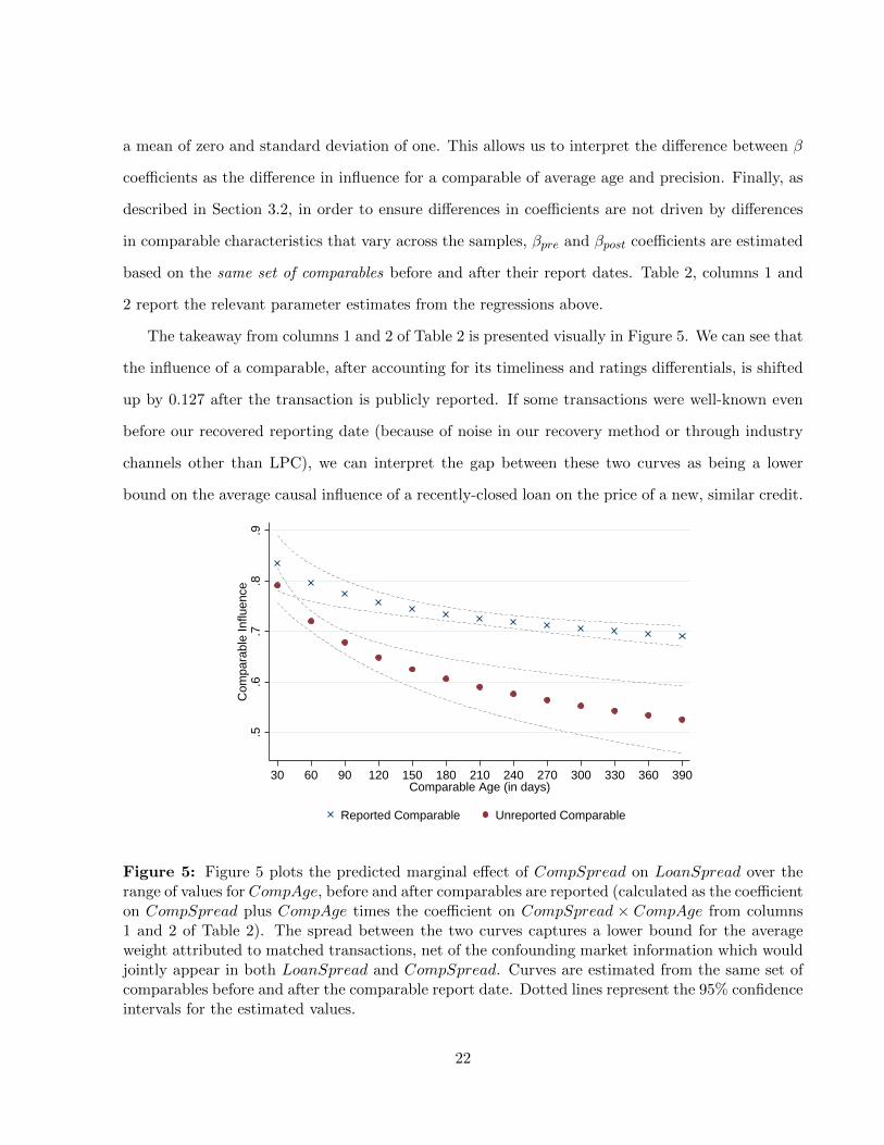
The takeaway from columns 1 and 2 of Table 2 is presented visually in Figure 5. We can see that

the influence of a comparable, after accounting for its timeliness and ratings differentials, is shifted

up by 0.127 after the transaction is publicly reported. If some transactions were well-known even

before our recovered reporting date (because of noise in our recovery method or through industry

channels other than LPC), we can interpret the gap between these two curves as being a lower

bound on the average causal influence of a recently-closed loan on the price of a new, similar credit.

.5.6

.7.8

.9C

ompa

rabl

e In

fluen

ce

30 60 90 120 150 180 210 240 270 300 330 360 390Comparable Age (in days)

Reported Comparable Unreported Comparable

Figure 5: Figure 5 plots the predicted marginal effect of CompSpread on LoanSpread over therange of values for CompAge, before and after comparables are reported (calculated as the coefficienton CompSpread plus CompAge times the coefficient on CompSpread × CompAge from columns1 and 2 of Table 2). The spread between the two curves captures a lower bound for the averageweight attributed to matched transactions, net of the confounding market information which wouldjointly appear in both LoanSpread and CompSpread. Curves are estimated from the same set ofcomparables before and after the comparable report date. Dotted lines represent the 95% confidenceintervals for the estimated values.

22

In the remaining columns of Table 2, we combine the two regressions by allowing the coefficient

on CompSpread to vary based on whether the comparable has been reported. That is, we estimate:

LoanSpreadi =α+ β1CompSpreadj + β2CompSpreadj ×Reportedi,j

+ β3Reportedi,j + γControlsi,j + εi,j

(5)

In column 3, we find the difference, captured in the coefficient on CompSpread× ReportedComp,

is economically and statistically significant at 0.103. Going from columns 1–2 to 3, we have also

forced the decay rates in comparables over time and across ratings to be the same for reported

and unreported transactions. While, as we discuss later, we have reason to think that the reported

transactions will have different dynamics, note that allowing the coefficients on CompSpread ×

CompAge and CompSpread×CompPrecision to differ in columns 1 and 2 doesn’t materially impact

the coefficient of interest. Moreover, we fail to reject a test that the coefficients on CompSpread×

CompAge and CompAge are jointly equal across columns 1 and 2 (and similarly for CompSpread×

Precision and Precision). Thus, going forward, we will generally lean on the more parsimonious

specification.

Column 4 replaces CompAge with more flexible dummy variables based on comparable age

(in months) with minimal effect on the interaction CompSpread×ReportedComp. We emphasize

this specification choice in particular because, in theory, this could be an important source of

confounding variation. Because, by definition, comparables can never be ‘unreported’ once they

are ‘reported’, CompAge naturally covaries with ReportedComp. Thus, the manner in which we

control for comparable age could potentially have a large bearing on the coefficient on CompSpread×

ReportedComp. However, we find the estimated influence of a comparable to be invariant to allowing

for a non-parametric decay function for comparable age.

Column 5 pushes the ‘within-comp’ identification strategy to its limit by estimating the spec-

ification in column 3 with the additional inclusion of 2,990 comparable fixed effects. Although

the coefficient of interest attenuates substantially in terms of economic significance, dropping from

0.103 to 0.058, the difference is not statistically significant.14 Going forward, we are careful to show

14Meanwhile, Griliches and Hausman (1986) (among others) shows that the inclusion of fixed effects may mechan-

23

results with and without the inclusion of comparable fixed effects where appropriate.

One way to interpret the economic magnitude of our estimates is to consider the propagation

of any hypothetical pricing errors that might affect a given loan. To do so, consider the following

back-of-the-envelope calculation. Since today’s loans become tomorrow’s comparables, if each loan

is priced using X number of comparables, then the average loan will also influence X number

of loans subsequently. In our sample, for example, this number is roughly five. As mentioned

above, our conversations with bankers suggest that a typical transaction might consider 3–7 similar

deals as comparables. Thus, the average loan will also be considered as a comparable for 3–7

transactions. As a result, any pricing error on a given loan will be propagated directly to 3–7

subsequent loans. More importantly, however, the pricing errors induced in those 3–7 loans will

spillover to an additional 9–49 loans, and so on. The multiplier effect generated by an individual

pricing error under comparables pricing can be approximated by 11−NumberofComps×wcomp , where

wcomp is the average causal influence of a comparable.15 Taking wcomp = 0.10 as a rough estimate

from Table 2 and assuming three comparables are used to price a loan, for example, the multiplier

effect is 1.4 times as large as the effect of the initial mispricing. Assuming lenders use 5–7 comps,

combined direct and indirect effects are 2.0–3.3 times as large as the direct effects on their own.

Recall that, for a variety of reasons, we should interpret the coefficients from Table 2 as lower bounds

on the influence of a comparable. As a result, the economic magnitudes discussed here should also

be interpreted as lower bounds. It seems reasonable, then, to expect the aggregate effects of a given

loan’s mispricing on all borrowers to be around twice as large as the effect on the directly-impacted

borrower due to the practice of comparables pricing.

To put these multipliers into context, consider recent papers in finance and economics suggesting

that interest rates charged by lenders may reflect concerns which go beyond the scope of the current

borrower’s creditworthiness. Ivashina (2009), for example, documents that information asymmetry

between the lead arranger of a loan and the syndicate explains variation in loan spreads. Her

discussion of economic magnitudes suggests typical variation in loan spreads resulting from this

ically amplify attenuation bias due to measurement error, in particular when the error is negatively auto-correlatedwithin a cross-sectional unit, as is likely the case in our setting.

15This follows from noting the summation of the pricing errors is a geometric series.

24

channel would amount to 29 basis points (see paper for a deeper discussion). Chodorow-Reich

(2014), meanwhile, documents a bank-credit channel in which distressed lenders charge higher rates

for relationship borrowers. Representative variation in lender distress, he shows, drives as much as

48 basis points in additional borrowing costs for matched borrowers. The analysis suggests these

effects drive hiring decisions at these firms.

While these magnitudes are non-trivial on their own, our analysis above would suggest the

spillover effects of pricing errors on subsequent transactions by other firms may be at least as large,

potentially much larger. For example, the substantive 48 basis point increase in borrower spreads

documented in Chodorow-Reich (2014) would translate into a cumulative interest rate effect of

68–160 basis points when spread among indirectly affected borrowers.

So, although it may be widely accepted that comparables play a role in a variety of markets, Table

2 suggests their direct and indirect spillover effects on equilibrium prices are large in magnitude. The

results also, however, establish the validity of using loans’ reporting dates as a source of variation

for comparable observability. This is a crucial ingredient in our forthcoming tests to determine

whether comparables are being used appropriately.

4.2 Tests of naıve use of comparables

We now turn our focus the question of whether the use of comparables in practice looks like optimal

information aggregation or naıve herding. To this point, none of the results documented above imply

the mistaken use of comparables. Pricing spillovers are collateral damage from an environment

with imperfect information. Yet, as we discussed in Section 2, using comparables appropriately

in realistic information environments would be difficult. Lenders would need not only to identify

like transactions for use in pricing, but also recover the basis under which those transactions were

priced. In our setting, this requires, at a minimum, that lenders know exactly the path of influence

from one loan to another for the entire history of interdependent transactions. Prima facie, this

seems unlikely.

If, instead, lenders naıvely treat past transactions as if they were independent signals, compa-

rables pricing will result in predictable empirical patterns in which redundant information across

25

comparables is consistently overweighted. The first such empirical pattern that we examine is how

the influence of a comparable evolves with repeated use. As a comparable is used repeatedly, the

possibility arises that it will have both direct and indirect influence on new transactions. If agents

fully take into account the multiple paths of influence, then we would expect the influence of a

comparable to be flat as it is used by more and more subsequent transactions, controlling for any

decrease in influence due to the passage of calendar time. On the other hand, if agents fail to correct

for the possibility that a given loan has directly influenced subsequent loans which are also being

used as co-comparables, then we would expect to see the total influence of a loan actually grow in

transaction time. That is, as it sequentially influences more and more transactions, naıve lenders

will give direct weight to the loan based on its role as a comparable, but also inadvertently allow it

additional indirect influence as a progenitor of subsequently closed comparables.

Table 3 provides evidence consistent with the latter effect. Returning to the set-up and basic

controls used in Table 2, we replace the dummy for whether or not a comparable has been reported

with a set of dummies that indicate the number of transactions the comparable has been linked

to both before and after being reported, allowing us to trace the evolution of influence based on

repeated use within a given comparable. In columns 1 and 2, the specification is:

LoanSpreadi =α+ βCompSpreadj +∑k

βpre,kCompSpreadj × PreMatchNumberKi,j

+∑k

βpost,kCompSpreadj × PostMatchNumberKi,j + γControlsi,j + εi,j ,

(6)

where the controls, as before, include CompAge and CompPrecision interacted with CompSpread

as well as level effects for any interacted variables. The omitted category is the first match pre-

reporting, such that in column 1, for example, the coefficient on CompSpread captures the co-

variation of the average comparable with the first subsequent transaction to which it is matched

before it has been reported. The interactions of CompSpread × 2ndMatch(Unreported) and

CompSpread × 3rdMatch(Unreported) test whether or not influence is growing before the trans-

action has been reported. The absence of any trend here is reassuring in that, even under gross

misuse of comparables, redundancy should not take effect until after the loan has been reported.

26

In contrast, the coefficients on CompSpread × 1stMatch(Reported) through CompSpread× ≥

5thMatch(Reported) increase monotonically. The difference in influence from the first time a com-

parable is used to the fifth is 0.083, significant at the 1% level and more than double the initial

influence. These findings are plotted graphically in Figure 6. The pattern of influence resembles a

kinked hockey stick, with a flat region before the comparable is reported, a jump due to the initial

influence the first date it is reported, and a trend based on repeated use thereafter.

.5.5

5.6

.65

.7.7

5.8

.85

Com

para

ble

Influ

ence

1st m

atch

(un

repo

rted

)

2nd

mat

ch

3rd

or la

ter

mat

ch

1st m

atch

(re

port

ed)

2nd

mat

ch

3rd

mat

ch

4th

mat

ch

5th

or la

ter

mat

chFigure 6: Figure 6 plots the coefficients for CompSpread × nthMatch in column 1 of Table 3,documenting the evolution of comparable influence with each subsequent match to a newly pricedtransaction, both before and after the comparable was reported.

Column 2 estimates the same pattern with comparable fixed effects. It is important to emphasize

here that any baseline variation in influence associated with a given comparable which could be

plausibly correlated with the number of matches assigned to it is netted out of the estimation by way

of fixed effects. That is, the difference in CompSpread×1stMatch(Reported) and CompSpread× ≥

5thMatch(Reported) of 0.060 (significant at the 5% level) captures the change in influence for a

given comparable based on potential for repeated use and not the difference in influence across

comparables based on the frequency with which our algorithm finds matches.16 Columns 3–5

16As a second point of emphasis here, recall that our assigned matches are based on our own algorithm designed to

27

estimate linear trends in influence before and after reporting for the same set of comparables.

Again, in column 3, we see no evidence that matching repeatedly to subsequent loans is associated

with additional influence. It is not until after the comparable is reported in columns 4 and 5 (with

and without comparable fixed effects) that the trend in influence emerges.

The growth in comparable influence based on its multiplicity of links to related loans observed

in Table 3 would seem consistent with the hypothesis that lenders are bad Bayesians who fail to

account for redundant information. At the same time, note that our sharpest prediction regarding

the risk of redundancy has to do with the number of potential paths for redundancy, not the simple

count of how many times the transaction has been used. For example, if a comparable has been

used four times before matching to its fifth transaction, then it will have at least five potential paths

of influence so long as each of the prior four transactions has been reported. On the other hand, if

none of the intervening transactions have been reported by the time the fifth transaction is priced,

the comparable can only have a direct path of influence, limiting the possibility of inadvertent

overweighting.

Following this line of reasoning, Table 4 sharpens our tests of boundedly-rational use of compa-

rables by tracking specific paths of influence and exploiting variation in the potential for redundancy

based on reporting delays of intervening transactions. For concreteness, consider the picture pre-

sented in Figure 7. A, B, and C represent three related transactions, each of which might be

identified as an informative comparable for the others. The timing of transactions is such, however,

that A precedes B which precedes C. Finally, assume that A was publicly reported in time to be

used by C, but perhaps not in time for B. Moreover, B may or may not have been reported in time

to be used in the pricing of C. These variations are captured in the figure with solid lines (implying

a given comparable was reported in time for use) and dotted lines (implying it was not). For the

triplet (i), note that there is a path for redundancy. Transaction A can be used both directly by

C, but also may exert indirect influence by way of B. In contrast, for triplets (ii) and (iii), the

potential for inadvertently overweighting A′ is shut down, either because A′ was not reported in

approximate the matches a banker might have chosen for a given deal and not the actual comparables used. Hence, ifsome transactions are unobservably more relevant and, as a result, used more frequently in practice by bankers, thatvariation would not show up in the number of matches captured by our algorithm.

28

time to influence B′ (as in (ii)) or because B′ was not reported in time to influence C′ (as in (iii)).17

A' B'

C'

βNR

A B

C

βR

A' B'

C'

βNR

(i) (ii) (iii)

Figure 7: Redundant comparables. The figure lays the framework for our tests of redundancybias. A, B, and C represent loan transactions. Solid arrows drawn between loans reflect directionalinfluence, so the line between A and C, for example, suggests that A was a viable (publicly-known)comparable for transaction C. In scenario (i), then, A has influence on C both directly and indirectlythrough B. We refer to A as a Redundant comparable for C, and βR represents the total influence ofA on C. Dotted arrows indicate that our algorithm matched the comparable to the new transactionbut that the comparable was not reported in time to actually influence the new transaction. To theright of the vertical line, then, no redundancies occur. In scenario (ii), there is no redundant pathof influence from A′ to C′ because A′ was not reported in time to influence B′. Similarly, A′ is notredundant for C′ in scenario (iii) because B′ was not reported in time to influence C′. We call A′ anon-redundant comparable for C′ and represent its influence with βNR.

To understand the sophistication of the lender, our question revolves around how much total

influence transaction A has on C relative to the influence transaction A′ has on C′. If lenders

incorrectly treat A and B as independent signals, any information contained in the pricing of loan

A will be duplicated in B and therefore overweighted by C. Thus, a naıve treatment of comparables

will see βR > βNR, as the total influence of A on C aggregates the direct influence and the indirect

influence through B. We refer to this as redundancy bias.

Finally, as the figure suggests, the potential for redundancy will be driven by the interaction of

reporting times for both the comparable in question (A) as well as its co-comparables (B). Prior

tests have largely depended on the assumption that variation in reported status of a comparable is

as-good-as-random within a given comparable. But by exploiting the reporting delays associated

17Of course, the path of redundancy would also be closed in the case that A′ was not reported in time for B′ andB′ was not reported in time for C′. This case is included among the non-redundant observations in our regressions inPanel A of Table 4 but was omitted from Figure 7 for ease of exposition.

29

with B transactions, we are afforded a shock to the potential for redundancy which is independent

of the comparable’s report date.

To implement the tests described above, we begin by searching our matches of loans and their

comparables (as described in Section 3.2) for the relationships shown in Figure 7. Specifically, we

identify loan triplets {A,B,C} such that A was used as a comparable for B and C, and B was also

used as a comparable for C. We compare these sets of loans to alternative triplets {A′,B′,C′} with

identical linkages except that at least one of the indirect links (A′ → B′ or B′ → C′) is shut down

because the comparable was not reported in time to be used by the new transaction. Of course,

we also encounter cases in which A has the potential for indirect influence on C through more than

one intervening loan (i.e., multiple B transactions that closed between A and C chronologically). A

comparable is deemed Redundant when it has an indirect effect through at least one such sibling

transaction.

The spirit of our tests closely matches that of tests in Tables 2 and 3. Specifically, after identi-

fying transactions matching the description above, we regress the spreads of transactions C on the

spreads of comparable transactions A interacted with a redundancy dummy:

LoanSpreadi =α+ β1CompSpreadj + β2CompSpreadj ×Redundanti,j

+ β3Redundanti,j + γControlsi,j + εi,j

(7)

We either estimate this in a single model with an interaction term as above, or in separate models

with separately estimated coefficients on controls. In either case, as before, we include controls for

the age of a comparable interacted with CompSpread, as well as the precision of the comparable and

its interaction. Finally, consistent with the within-comparable estimation applied in Tables 2 and

3, we wish to compare the same comparable, before and after it is made redundant via intervening

transactions.

Columns 1 and 2 of Table 4 begin by comparing the influence of the same set of comparables

on subsequent transactions before and after a redundancy arises across two separately estimated

regressions. The difference in coefficients on CompSpread suggests that the availability of additional

paths of influence increases comparable influence by 0.034. Similar magnitudes are seen on the

30

interaction between CompSpread and Redundant in the combined specifications in columns 3 and

4, with and without comparable fixed effects. Finally, columns 5 and 6 take advantage of the

variation in the number of paths of influence that a given comparable has over a new transaction

by breaking the Redundant dummy into a set of dummies based on the number of redundant

paths. For example, referring back to Figure 7, A will have two redundancies for C if there are

two different B transactions that satisfy the redundant relationship in scenario (i). We see that

influence grows with each additional redundancy, growing from 0.015 with the first redundancy to

0.077 by the fourth redundancy in column 5 and by similar magnitudes in column 6, where we

include comparable fixed effects.

Finally, as mentioned above, a second benefit of tracing out the full path of influence of a

comparable through potential co-comparables is that it allows us to isolate variation in the potential

for redundancy which is unrelated to the comparable’s own reported status. To this point, our

identification strategy has leaned on the assumption that the comparable’s informativeness about

fundamentals is fixed over time, or at least quasi-random with respect to its report date. In Panel

B, however, we are able to go one step further. Rather than relying on the reported status of both

A and B, we instrument for Redundant using only the reported status of B with respect to C and

even control for reporting delays associated with A. Even if a comparable’s appropriate influence is

changing over time in way that is correlated with its own report date, we will be able to identify

the causal effect of redundancy as long as its informativeness is independent of its co-comparables’

report dates.

Columns 1 and 2 of Panel B re-estimate the regressions from columns 3 and 4 of Panel A. This

time, however, we instrument for Redundant using an indicator equal to one when redundancy is

prevented because no B transactions were reported in time to be used by C (as reflected in scenario

(iii) of Figure 7). Call this indicator DelayedB for reference. We further use CompSpread ×

DelayedB as an instrument for CompSpread×Redundant (Wooldridge 2010).18

With the variation in redundancy fully isolated to the reporting status of B transactions, we

18The two implicit first-stage regressions are omitted in the main text for brevity, but included in Table A2 of theappendix. Not surprisingly, however, DelayedB serves as a powerful instrument for Redundant, with an F-stat inthe first stage for Redundant of 166, significant at the 1% level. Similarly, the associated F-stat for CompSpread×DelayedB in the first stage for CompSpread×Redundant is 484, significant at the 1% level.

31

can control for the reporting delay associated with A (in log days between the transaction and its

report date) and its interaction with CompSpread, which we do in column 1. In column 2 we soak

up this variation with comparable fixed effects. In either case, our findings are consistent with

the magnitudes presented in Panel A, with the instrumented effects of redundancy increasing a

comparable’s influence by 0.052, with or without fixed effects.

An alternative, more restrictive approach to these tests, meanwhile, might be to simply limit

the sample to scenarios (i) and (iii) in Figure 7, where the A comparable was reported in time for

its B co-comparables. Within this restricted sample, the only source of variation in redundancy is

the reported status of B transactions (the IV and OLS strategies are equivalent in this subsample

since DelayedB moves one-for-one with Redundant). Moving to the restricted subsample drops

12,613 observations for which the comparable under investigation was not reported in time for

its potentially-intervening B transactions. The interaction Redundant × CompSpread remains

positive, significant, and largely unchanged across various specifications. In Column 3, we estimate

the regression from Equation 7. In Column 4, we add controls for comparable A’s own reporting

delay, interacted with CompSpread, while in column 5 we add comparable fixed effects. Finally,

column 6 reports the growth in influence based on the number of redundancies, again including

comparable fixed effects.

In addition to providing plausibly exogenous variation in the potential redundancy of a com-

parable, the tests in Panel B of Table 4 also help to rule out an otherwise reasonable alternative

hypothesis. Viewed in isolation, Panel A cannot rule out the possibility that lenders are aware of

the risk of redundancy in their comparables but lack the information on loan observability needed

to correct for it. Referring back to Figure 7, it may be that a lender in scenario (i) or (ii) recognizes

the potential for redundancy but is unsure whether or not A was reported in time for B. Given this

uncertainty, a sophisticated lender could choose weights such that A would receive too much weight

in case of an actual redundancy (scenario (i)) and too little weight in the absence thereof (scenario

(ii)), but just the right weight on average (scenarios (i) and (ii) together).19

19Of course, it is also not clear why lenders should have less information than the econometrician in this setting.Actual comparable report dates could be generated in real time by any banker who valued them simply by recordingadditions to the LPC database feed in real time.

32

To test whether A receives the right weight on average when the lender perceives a possible

redundancy, we might pool the potentially redundant scenarios (i) and (ii) and compare them to

scenario (iii), in which there is no apparent risk of redundancy. This is exactly what is done by the

instrumental variables specifications in Panel B. This is perhaps easiest to see by examining the

reduced-form regression corresponding to column 1 of Panel B (reported in column 3 of Table A2

in the appendix). By isolating the variation in redundancy to that which comes from the reported

status of B transactions, we are effectively comparing scenarios (i) and (ii) to scenario (iii). The

negative coefficient on DelayedB in the reduced-form (or the corresponding positive coefficient in

the IV regressions) suggests lenders don’t just place excess weight on comparables known to the

econometrician to be redundant—on average, they overweight the set of comparables which they

themselves should recognize to be potentially redundant, even absent information on reporting

dates. This, in turn, implies that pricing errors are due to more than just incomplete information

on when loans were made available to rival lenders for use as comparables. Lenders are not getting

things right on average, but instead make gross errors in information aggregation consistent with

redundancy neglect.

In summary, across a variety of samples and specifications above, we find that allowing the

possibility of a redundant path of influence increases the influence of a given comparable by 0.028–

0.052. To put these magnitudes in perspective, recall that our earlier tables estimated the influence

attributable to a single comparable to be between 0.058 and 0.104. Hence, when compared to the

baseline influence estimated in Table 2, redundancy neglect appears to play a large role in price

formation.

4.3 Naıve comparables and aggregate dynamics

Our final tests go further in demonstrating the degree to which comparables represent a form of

naıve inference and broaden the scope of errors users make. Recall from the examples in Section 2

that common information will tend to be overweighted based on naıve use of comparables. In

Tables 3 and 4, common information is shared among comparables based on the recursive use

of those comparables. While this is a natural mechanism for generating excess weight on some

33

information at a given point in time, correcting the mistake requires lenders to know exactly what

comparables were used, when they were used, and by whom.

Now we consider the history of market-wide macroeconomic information from equity and bond

markets as a source of common information about fundamentals—in particular, Baa–Aaa bond

spreads, the market dividend/price ratio, and the VIX index—and test the extent to which naıve

inference dictates the dynamic relationship between loan spreads and aggregate conditions. We focus

on price signals which are widely available and likely constitute relevant information to the lender

pricing a new loan, just as they would have been used by lenders setting terms for comparables. Yet,

just as we documented that naıve inference might lead a lender to mis-weight the history of past

signals by improperly accounting for their recursive use, the same risk looms large with aggregate

signals. Standing at time t, a lender forms his opinion about fundamentals by examining the entire

history of news. This may involve placing positive weight on aggregate levels of Baa–Aaa spreads

from the prior month either implicitly (by weighting current Baa–Aaa spreads, which are highly

persistent) or explicitly. Yet, if in addition to his best guess of fundamentals based on this history

of aggregate news he also weights comparables from the prior month, he may fail to account for

the fact that his comparables were also largely influenced by the then-contemporaneous Baa–Aaa

spread. Naıve inference generates the prediction that, holding fundamentals constant, loans for

which the relevant comparables occurred in good times will benefit from more attractive terms.

News about fundamentals will have a persistent effect on prices, where the persistence depends on

the frequency with which transactions are completed and used as comparables.

Table 5 asks the following: at a given point in time, can cross-sectional variation in loan spreads

be explained by variation in the aggregate conditions prevailing at the time relevant comparables

were priced? Using the matching methods employed in the previous tables, we generate a sample of

matched comparable × loan pairs, this time limiting ourselves to matches which were reported in

time to be used as comparables for the current loan. For each loan, we compute the average logged

spread of that loan’s comparables, as well as the average of Baa–Aaa spreads, the dividend/price

ratio of the S&P 500, and the VIX prevailing at the time each comparable was priced (we again

34

assume loans were priced one month prior to closing).20

For example, assume credit spreads in September, October and November are 75, 100 and 150,

respectively. For a loan being priced in January (loan 1) using comparables priced in November

and October, we would calculate the average spreads prevailing at the time of its comparables as

125. The spirit of our test will be to compare loan 1 to another simultaneously priced loan (loan

2) for which we identify comparables which were priced in September. For loan 2, prevailing credit

spreads at the time its comparables were priced were just 75.

Based on the differences in aggregate conditions prevailing at the time comparables closed,

we would, of course, expect that the comparables for loan 1 will have higher spreads than those

for loan 2. This is testable, and we report this is the case in Panel A of Table 5. And while

lenders setting rates for loans 1 and 2 may optimally wish to use the full history of Baa–Aaa

spreads in setting new prices, in doing so, they will need to account for the fact that that October

and November’s information was already reflected in the spreads of loan 1’s comparables, while

September’s information was already embedded in the spreads of loan 2’s comparables. Any evidence

of cross-sectional variation in loan spreads based on the prevailing macroeconomic conditions at the

time of comparables’ closing would strongly indicate a gross error in the interpretation and use of

information embedded in comparables.

We report our findings in the form of two stage least squares (2SLS). As opposed to the tradi-

tional motivation for 2SLS as a remedy for endogenous covariates, we use the methodology instead

to track and isolate the path of influence of aggregate macroeconomic news. The first stage shows

the effect of macroeconomic news on a set of comparables. The second stage shows how that effect,

in turn, is transmitted into variation in subsequent loan spreads.

The first stage of the 2SLS is presented in Panel A of Table 5. The unit of observation is the

primary loan being priced, where each loan has been matched to an average of five comparables

following the methodology described in Section 3.2. Only comparables which were reported in

time to be used are included. The dependent variable in the first stage is the average log spread of

comparables we have identified for each loan. The variation of interest is that of prevailing Baa–Aaa

20Baa–Aaa spreads and the VIX are taken from the St. Louis Federal Reserve Bank data repository and are monthlyaverages. The D/P ratio of the S&P 500 was taken from Bob Shiller’s website.

35

spreads, the S&P 500 dividend/price ratio, and the level of the VIX in the month that comparables

were priced, averaged over all the comparables for a given loan.

In the first stage, we include all controls that we will need in the second stage, including rating

and industry fixed effects for the borrower being priced, along with a control for the log of loan size

(in dollars) and log of loan maturity (in months). We also include time fixed effects at the monthly

frequency, where timing is tied to the closing date of the loan being priced. Many of these controls

are motivated by the second stage. We will return to a discussion of them shortly.

Columns 1–4 of Panel A demonstrate the unsurprising link between the various market indicators

and contemporaneous spreads on loans to be used as comparables. In columns 1–3 we find that

Baa–Aaa bond spreads, D/P levels, and the VIX positively covary with the spreads chosen for

loan market borrowers. Column 4 includes all indicators jointly. At the bottom of the table, we

report the F-statistic testing for significance of the excluded instruments. In each case, they exceed

standard rules of thumb (Staiger and Stock 1997) as well as 10% critical values for maximal IV size

based on Stock and Yogo (2005).

Though the results here are not surprising, they confirm that the macro variables chosen influence

contemporaneous loan spreads and with the right signs. High bond spreads generate high loan

spreads. Loans priced in periods of low valuation (high D/P) and high volatility also have higher

loan spreads. Without sufficient influence of aggregate information on the loan market here, we

could not reasonably proceed to test whether or not that information was incorrectly overweighted

later by way of comparables.

The results from Panel B, on the other hand, are more surprising. In the second stage, we now

regress the log spread chosen for the new loan on the average log spread, where averages are taken

over multiple comparables. But, by construction and the mechanics of 2SLS, the variation in the

average spread of the comparables is limited to that which comes from our first stage instruments

used in Panel A (any other source of variation in the fitted values from the first stage is absorbed

by the inclusion of the full set of controls). In other words, column 1 tells us how new loan pricing

is impacted by variation in the pricing of comparables which comes from the Baa–Aaa spread at

36

the time of each comparable.21

Before discussing the results, an important aspect of the test we wish to highlight is the presence

of monthly fixed effects as of the date of the loan being priced. By including time fixed effects, we

can be agnostic about the appropriate use of lagged macroeconomic news. Because the history of

lagged macroeconomic news will be the same for all loans priced in a given month, the fixed effects

absorb that information completely without needing to specify a particular lag structure. The only

variation remaining comes from the timing of when comparables for a given loan occurred. The

coefficients in Panel B tell us the extent to which a loan puts excess weight on stale information

based on the timing of its comparables.

Looking across columns 1–4 of Panel B, we see the different effects based on different instrument

choices (each column corresponds to the first stage regression reported in the same column from

Panel A). Column 1, for example, uses Baa–Aaa spreads occurring in the month of comparables as

the sole instrument. We find that a doubling of the average spread on comparables due to aggregate

variation in Baa–Aaa spreads at the time of the comparable (holding fixed contemporaneous bond

spreads) translates into a 33.7% increase in the affected loan’s spread relative to loans priced at

the same point in time but based on different comparables. Columns 2 and 3 repeat the exercise

using the dividend/price ratio and the VIX and find larger and more significant effect sizes. Finally,

column 4 uses all three instruments jointly. A doubling of comparable spreads based on common

macro signals coming from bond and equity markets increases spreads for loans priced based on

those comparables by 56.7%.22

As in Tables 3 and 4, the evidence suggests excess weight is placed on the correlated information

contained in comparables, this time due to presumably stale macroeconomic information. But what

if loan prices should contain the stale information documented above, or the ‘stale’ information

from the time of transaction comparables is more relevant than we think? For example, sleepier

segments of the market will have comparables arrive with a longer lag. If the same segments also

21We have chosen to use the 2SLS framework because it provides information on the full path of influence of theaggregate information, but we might have alternatively just reported reduced form regressions of loan spreads on theinstruments. Such an exercise would mechanically generate coefficients exactly equal to the product of our first- andsecond-stage coefficients.

22This result does not appear to hinge importantly on any specific time period. In unreported results, the effect isminimally changed if we focus on the financial crisis (2008–2009) or if we exclude the crisis from our sample.

37

respond to macroeconomic conditions with a similar lag structure, the patterns in Table 5 may

not reflect pricing errors at all. In other words, without random arrival rates of comparables, it

is difficult to rule out endogenous matching between the timing of comparables and sensitivity to

macro fundamentals.

To help sort this out, our last results track the ex-post performance of the loans being priced

based on the lag structure motivated above. Using a subsample of loans which trade in the secondary

market after being priced in the primary market, we calculate the percentage capital appreciation

on the loan between the month after the loan closed and 3, 6, 9 or 12 months thereafter. To be

conservative, we ignore the component of loan returns attributed to the affected interest rates and

focus only on price changes, although results are consistent when loan coupon payments are added

to the return. In the event the loan is not traded in the secondary market in the month following the

closing date, we instead calculate capital appreciation as the percentage change in price relative to

par or, if the loan was issued at a discount, the percentage change in price relative to its discounted

issue price over the corresponding time horizon.

Data on loan values come from mark-to-market quotes aggregated across dealers by the Loan

Syndications and Trading Association. We match these to DealScan using a matching file of deal

identifiers provided by Thompson Reuters and some data cleaning. For example, we drop facilities

for which the issuance dates across the two data sources differ by more than 60 days. We also

drop loans which appear to trade in advance of their DealScan closing date. We should be wary

that any test that relies on an active response to mispricing in the secondary loan market may

be hampered by stale loan quotes provided by dealers. At the same time, other work suggests a

surprising amount of efficiency in the secondary loan market. Addoum and Murfin (2017) show that

dealer quotes on secondary loans may even lead the corresponding equities of the same firm. We

also caveat the analysis by emphasizing that any evidence of predictability by no means suggests a

profitable trading strategy. Dealer quotes are not firm and transaction costs may be large. Instead,

our tests might be conservatively interpreted as capturing changing dealer opinions about the value

of loans after the time of purchase.

In Panel A, we repeat the first stage regression from column 4 of Table 5 to confirm that,

38

even in the limited sample of traded loans, the spreads of the loans’ comparables are predicted by

prevailing macroeconomic conditions at the time they closed. Unlike the prior results, the effect

of credit spreads is crowded out in the first stage, but otherwise, dividend to price and volatility

provide a strong first stage to generate variation in issuance spreads based on comparable conditions.

In Panel B, we present the second stage results, which suggest that in the 6, 9, and 12 months after

the loan closes, dealer quotes adjust based on the variation in spreads. A doubling of comparable

spreads due to prevailing macro conditions predicts 4–6% appreciation in the loan’s value in the 6,

9, and 12 months post issuance. These are non-trivial effect sizes. Twelve month returns on the

loans have a standard deviation of just 8%.

Taken together, Tables 5 and 6 document the patterns we might expect from a boundedly-

rational use of comparables that fails to take into account overlapping information. Over time,

loans which were overpriced at the time of issuance tend to fall in value, and vice versa, confirming

that the patterns of comparable use present direct evidence of mispricing. These results complement

the findings from earlier tables in several ways. First, they again distinguish between an imperfect

but still sophisticated use of comparables in which lenders weight comparables such that spreads

are right on average, but sometimes overweight and sometimes underweight past information based

on the history of comparable use. In such a world, we might think that the cost of tracking who

used which comparable in order to make corrections for signal redundancy is simply too large.

Yet whereas the presumption of common knowledge about the history of comparables use may be

too large an information burden for even sophisticated users of comparables, common knowledge

regarding use of market-wide information should not be. Even boundedly-rational lenders should

assume that lenders setting terms at t−1 would have used this information. Thus, the evidence that

aggregate movements in bond or equity markets occurring at the time of a comparable’s closing have

undue influence over the subsequent loans priced using that comparable suggests a gross pricing

error.

Table 5 also contributes to our understanding of the complicated dynamics in asset prices which

are induced by the use of comparables. Even the correct use of comparables would suggest prices

will reflect a moving average of lagged fundamentals. This is consistent with the tendency for

39

average loan spreads to be smoother than bond market yields. That phenomenon, however, might

also reflect the smoothing benefits of relationship banking, where lenders overcharge in good times

in order to hedge borrowers against bad times.

Yet the more complicated dynamics implied by Table 5 suggest that, because lenders incorporate

stale macroeconomic news through naıve use of comparables, current prices will tend to overweight

lagged fundamentals at the expense of other information. Prices are set based on a distributed lag

of aggregate news, where the lag length depends on when transactions relevant to the current batch

of new loans last closed.

5 Discussion

We have documented the practice and practical importance of comparables pricing in credit orig-

ination markets. We show that comparables play a quantitatively important role in the way that

credit is priced. Moreover, we find strong evidence that the use of comparables is a manifestation of

naıve inference, leading to predictable pricing mistakes and dynamics of credit spreads that depend

on the timing of comparables. Given the interest in how credit is allocated, priced, and perhaps

mispriced, this is an important avenue for examination.

However, the applications of comparables pricing are much broader. IPO markets, real estate,

mergers and acquisitions, private equity, and a host of secondary markets all rely heavily on this

pricing methodology. The primary lessons from our analysis may extend more broadly to these

markets. As the dominant pricing methodology in these markets, how significant is comparables

pricing as a driver of pricing dynamics?

The evidence of naıvete in the use of comparables suggests interesting policy questions going

forward. If agents were using comparables efficiently, then everyone would be made better off by

the availability of market information, since prices would be as accurate as possible given available

information. However, this is not necessarily true when agents use comparables naıvely. Are there

situations in specific markets in which opacity may actually improve pricing accuracy? We leave

this and other questions for future research.

40

References

Addoum, Jawad, and Justin Murfin, 2017, Hidden in plain sight: Equity price discovery with

informed private debt, Working Paper.

Banerjee, Abhijit V., 1992, A simple model of herd behavior, The Quarterly Journal of Economics

107, 797–817.

Bikhchandani, Sushil, David Hirshleifer, and Ivo Welch, 1992, A Theory of Fads, Fashion, Custom,

and Cultural Change as Informational Cascades, Journal of Political Economy 100, 992–1026.

Bordalo, Pedro, Nicola Gennaioli, and Andrei Shleifer, 2017, Diagnostic expectations and credit

cycles, Journal of Finance, forthcoming.

Chodorow-Reich, Gabriel, 2014, The employment effects of credit market disruptions: Firm-level

evidence from the 2008-9 financial crisis, The Quarterly Journal of Economics 129, 1–59.

Da, Zhi, and Xing Huang, 2016, Harnessing the wisdom of crowds, Working paper, University of

Notre Dame and Michigan State University.

Dell’Ariccia, Giovanni, and Robert Marquez, 2006, Lending booms and lending standards, The

Journal of Finance 61, 2511–2546.

DeMarzo, Peter M., Dimitri Vayanos, and Jeffrey Zwiebel, 2003, Persuasion bias, social influence,

and unidimensional opinions, The Quarterly Journal of Economics 118, 909–968.

Dougal, Casey, Joseph Engelberg, Christopher A. Parsons, and Edward D. Van Wesep, 2015, An-

choring on credit spreads, The Journal of Finance 70, 1039–1080.

Eyster, Erik, and Matthew Rabin, 2010, Naıve herding in rich-information settings, American

Economic Journal: Microeconomics 2, 221–43.

, 2014, Extensive imitation is irrational and harmful, The Quarterly Journal of Economics

129, 1861–1898.

41

Fama, E.F., and K.R. French, 1997, Industry costs of equity, Journal of Financial Economics 43,

153–93.

Glaeser, Edward L., and Charles G. Nathanson, 2017, An extrapolative model of house price dy-

namics, Journal of Financial Economics, forthcoming.

Gorton, Gary B, and Ping He, 2008, Bank credit cycles, The Review of Economic Studies 75,

1181–1214.

Graham, John R., 1999, Herding among investment newsletters: Theory and evidence, The Journal

of Finance 54, 237–268.

Greenwood, Robin, and Samuel G. Hanson, 2013, Issuer quality and corporate bond returns, Review

of Financial Studies 26, 1483–1525.

Griliches, Zvi, and J.A. Hausman, 1986, Errors in variables in panel data, Journal of Econometrics

p. 31:93118.

Ivashina, Victoria, 2009, Asymmetric information effects on loan spreads, Journal of Financial

Economics 92, 300–319.

Kim, Moonchul, and Jay Ritter, 1999, Valuing IPOs, Journal of Financial Economics 53, 409–437.

Murfin, Justin, and Mitchell Petersen, 2016, Loans on sale: Credit market seasonality, borrower

need, and lender rents, Journal of Financial Economics 121, 300–326.

Purnanandam, Amiyatosh K., and Bhaskaran Swaminathan, 2004, Are IPOs really underpriced?,

Review of Financial Studies 17, 811–848.

Rajan, Raghuram G, 1994, Why bank credit policies fluctuate: A theory and some evidence, The

Quarterly Journal of Economics pp. 399–441.

Rhodes, Tony, 2008, Syndicated Lending-Practice and Documentation (Euromoney) 5th edn.

Ruckes, Martin, 2004, Bank competition and credit standards, Review of Financial Studies 17,

1073–1102.

42

Staiger, Doug, and James Stock, 1997, Instrumental variables regression with weak instruments,

Econometrica 65, 557–586.

Stock, James, and Motohiro Yogo, 2005, Testing for Weak Instruments in Linear IV Regression .

pp. 80–108 (Cambridge University Press: New York).

Taylor, Allison, and Alicia Sansone, 2006, The Handbook of Loan Syndications and Trading

(McGraw-Hill Education).

Welch, Ivo, 1992, Sequential Sales, Learning, and Cascades, Journal of Finance 47, 695–732.

, 2000, Herding among security analysts, Journal of Financial Economics 58, 369–396.

Wooldridge, Jeffrey M., 2010, Econometric Analysis of Cross Section and Panel Data (MIT Press)

2nd edn.

43

Table 1: Summary statistics. The table reports means, medians and standard deviations of loan amount, maturity, rating,and interest rate spread in basis points. Panel A shows the statistics for the entire sample of loans and their matched comparablesas described in Section 3.2 along with a test for equality of means between the facilities being priced and the comparables. PanelB reports the same for the samples of comparables which were or were not reported in time for use. Panel C reports the statisticsfor the subset of comparables which match to subsequent transactions at least once before and after being reported. Panel Dcompares the characteristics of the facilities that match to those comparables from Panel C before they were reported vs. afterthey were reported, ignoring any transactions that matched to both. ***, **, and * indicate significance at the 1, 5, and 10%level, respectively.

Panel A Facilities priced Comparables

N Mean Median S.D. N Mean Median S.D. ∆ Means

Facility Amount ($M) 23,934 491.8 250.0 870.9 23,108 462.3 235.0 802.1 (29.5)***Maturity (months) 23,934 50.17 60 24.13 23,108 50.11 60 23.97 (0.06)Numerical Avg LT Debt Rating (2-24) 23,934 13.40 14 3.53 23,108 13.41 14 3.47 0.01Loan Spread 23,934 204.9 175.0 153.3 23,108 206.0 175.0 152.9 1.11

Panel B Unreported comparables Reported comparables

N Mean Median S.D. N Mean Median S.D. ∆ Means

Facility Amount ($M) 3,966 318.3 150.0 588.7 22,132 468.1 250.0 807.5 149.8***Maturity (months) 3,966 44.74 48 24.02 22,132 50.29 60 23.87 5.55***Numerical Avg LT Debt Rating (2-24) 3,966 13.37 14 3.39 22,132 13.41 14 3.47 0.04Loan Spread 3,966 183.6 150.3 136.6 22,132 206.4 175.0 152.9 22.8***

44

Panel C Switching comparables

N Mean Median S.D.

Facility Amount ($M) 2,990 313.6 150.0 565.2Maturity (months) 2,990 44.27 47 23.36Numerical Avg LT Debt Rating (2-24) 2,990 13.30 14 3.29Loan Spread 2,990 179.1 150.0 131.1

Facilities priced by Facilities priced byPanel D unreported comparables reported comparables

N Mean Median S.D. N Mean Median S.D. ∆ Means

Facility Amount ($M) 2,216 474.4 202.5 963.6 5,849 477.0 225.0 878.6 2.60Maturity (months) 2,216 46.10 53.5 24.22 5,849 47.22 55 22.66 1.12Numerical Avg LT Debt Rating (2-24) 2,216 13.11 14 3.49 5,849 13.25 14 3.44 0.14Loan Spread 2,216 183.9 150.0 144.7 5,849 189.8 175.0 140.4 5.90

45

Table 2: Comparable influence. The table estimates the influence of loan interest rate spreads for past closed loans (the“comparables”) on the spreads of subsequent, similar loans before and after the comparables were reported in a widely-usedtransactions database. Observations are at the level of loan × comparable. Spreads of the loans being priced and the comparablesare in logs. CompAge and CompPrecision reflect the logged distance in days and -log of 1+ the difference in numericalratings between the loan and the comparable. Both are standardized to have zero mean and unit standard deviation for ease ofinterpretation and are interacted with CompSpread in all but column 4. Column 4 controls for comparable age and its interactionwith comparable spread via dummies based on age in months. Column 5 includes comparable fixed effects. Standard errors arereported in parentheses and are clustered at the level of comparable firm and borrowing firm. ***, **, and * indicate significanceat the 1, 5, and 10% level, respectively.

Unreported ReportedComps Comps Combined

Loan Spread (1) (2) (3) (4) (5)

Comp Spread 0.610*** 0.737*** 0.638*** 0.635***(0.034) (0.015) (0.026) (0.041)

Comp Spread × Reported Comp 0.103*** 0.104*** 0.058***(0.026) (0.027) (0.020)

Reported Comp -0.447*** -0.444*** -0.309***(0.134) (0.139) (0.103)

Comp Spread × Precision 0.053*** 0.048*** 0.050*** 0.049*** 0.035***(0.015) (0.011) (0.010) (0.010) (0.009)

Comp Precision -0.256*** -0.222*** -0.235*** -0.231*** -0.165***(0.076) (0.057) (0.052) (0.052) (0.045)

Comp Spread × Comp Age -0.068*** -0.037*** -0.049*** -0.036***(0.017) (0.011) (0.010) (0.008)

Comp Age 0.297*** 0.166*** 0.217*** 0.193***(0.087) (0.058) (0.052) (0.042)

Comp Age Dummies (monthly) × Comp Spread NO NO NO YES NOComp Fixed Effects NO NO NO NO YESNumber of Comparables 2,990 2,990 2,990 2,990 2,990Number of Observations 5,433 11,886 17,319 17,319 17,319R-squared 0.471 0.514 0.500 0.501 0.770

46

Table 3: Repeated comparable use. The table measures the growth in influence of a comparableas it is matched to an increasing number of new transactions. Columns 1 and 2 interact CompSpreadwith dummies for the number of loans a comparables has matched to before and after being reported.The excluded category is the first pre-reported match. Column 2 adds comparable fixed effects.Columns 3 through 5 estimate the growth in influence parametrically by interacting the comparable’snumber of prior matches with CompSpread. Column 3 does this only for comparables before theyare reported, while columns 4 and 5 focus on the same comparables after they are reported, with andwithout comparable fixed effects. All regressions include controls for comparable age and precisionas well as their interactions with CompSpread, as described in Table 2. Standard errors are reportedin parentheses and are clustered at the level of comparable firm and borrowing firm. ***, **, and* indicate significance at the 1, 5, and 10% level, respectively.

UnreportedCombined Comps Reported Comps

Loan Spread (1) (2) (3) (4) (5)

Comp Spread 0.632*** 0.579*** 0.675***(0.033) (0.055) (0.024)

Comp Spread × 2nd Match (Unreported) -0.023 -0.024(0.029) (0.023)

Comp Spread × ≥ 3rd Match (Unreported) -0.037 -0.008(0.045) (0.028)

Comp Spread × 1st Match (Reported)a 0.066** 0.068***(0.030) (0.026)

Comp Spread × 2nd Match (Reported) 0.075** 0.071**(0.035) (0.031)

Comp Spread × 3rd Match (Reported) 0.130*** 0.104***(0.037) (0.035)

Comp Spread × 4th Match (Reported) 0.133*** 0.117***(0.042) (0.040)

Comp Spread × ≥ 5th Match (Reported)b 0.149*** 0.128***(0.047) (0.043)

(b)-(a) 0.088*** 0.060**

Comp Spread × Number Prior Matches -0.020 0.022*** 0.020**(0.027) (0.008) (0.009)

Number Prior Matches 0.079 -0.103** -0.106**(0.139) (0.041) (0.047)

Other Controls YES YES YES YES YESComp Fixed Effects NO YES NO NO YESNumber of Comparables 2,990 2,990 2,990 2,990 2,990Number of Observations 17,319 17,319 5,433 11,886 11,886R-squared 0.502 0.770 0.472 0.515 0.805

47

Table 4: Comparable redundancy. The table estimates the influence of closed loans on subse-quent matched transactions based on whether or not the loans were also likely influential for oneor more reported co-comparables for the same transaction, thereby providing an indirect path ofinfluence. We condition on a sample of loan × comparable pairs where the comparable was re-ported prior to its match (and thus was directly influential), but was also matched to at least oneco-comparable for the same loan. The indicator for Redundant is equal to one for comparables thatwere reported in time to influence at least one co-comparable and for which that same co-comparablewas reported in time to influence the transaction being priced. See Figure 7 for a visual descriptionand the text for details on sample construction. All regressions include controls for comparable ageand precision as well as their interactions with CompSpread, as described in Table 2. Columns 1and 2 compare the same comparables’ influence across redundant and non-redundant matches inseparate regressions, whereas columns 3 through 6 interact CompSpread with Redundant to testfor differences in influence. Standard errors are reported in parentheses and are clustered at thelevel of comparable firm and borrowing firm. ***, **, and * indicate significance at the 1, 5, and10% level, respectively.

Panel A Non-Redundant Redundant Combined

Loan Spread (1) (2) (3) (4) (5) (6)

Comp Spread 0.778*** 0.812*** 0.778*** 0.776***(0.012) (0.013) (0.012) (0.012)

Comp Spread × Redundant Comp 0.036*** 0.028**(0.013) (0.013)

Redundant Comp -0.172*** -0.157**(0.066) (0.065)

Comp Spread × 1 Redundancya 0.015 0.021(0.014) (0.013)

Comp Spread × 2 Redundancies 0.040*** 0.045***(0.015) (0.016)

Comp Spread × 3 Redundancies 0.063*** 0.064***(0.018) (0.020)

Comp Spread × ≥ 4 Redundanciesb 0.077*** 0.078***(0.022) (0.024)

(b)-(a) 0.062*** 0.057***

Other Controls YES YES YES YES YES YESComp Fixed Effects NO NO NO YES NO YESNumber of Comparables 5,108 5,108 5,108 5,108 5,108 5,108Observations 9,375 20,426 29,801 29,801 29,801 29,801R-squared 0.606 0.633 0.624 0.820 0.625 0.820

48

Table 4: Comparable redundancy, continued. Panel B focuses on the delay in reporting ofco-comparables as the source of variation in Redundant. In columns 1 and 2, this is done by instru-menting for Redundant using an indicator equal to one when a redundancy is prevented because noco-comparables were reported in time to influence the new transaction. The first-stage regressionsfor Redundant and Redundant × CompSpread, along with the corresponding reduced-form, arereported in Table A2 in the appendix. Column 1 controls for the reporting delay of the comparablein question (in log days) and its interaction with CompSpread. Column 2 includes comparablefixed effects. In columns 3 through 6, the effective control group (non-redundant comparables)is restricted to those comparables whose redundancy was shut down because of delayed reportingof their co-comparables. These tests effectively compare scenario (i) to scenario (iii) in Figure 7.Column 5 includes comparable fixed effects. Column 6 replaces Redundant with a set of dummiesbased on the number of redundant paths. All regressions include controls for comparable age andprecision as well as their interactions with CompSpread, as described in Table 2. Standard errorsare reported in parentheses and are clustered at the level of comparable firm and borrowing firm.***, **, and * indicate significance at the 1, 5, and 10% level, respectively.

Panel BInstrumental Variables OLS—Restricted Sample

Loan Spread (1) (2) (3) (4) (5) (6)

Comp Spread 0.785*** 0.779*** 0.764***(0.019) (0.015) (0.049)

Comp Spread × Redundant Comp 0.052** 0.052** 0.037** 0.037** 0.034**(0.023) (0.021) (0.018) (0.018) (0.017)

Redundant Comp -0.217* -0.278*** -0.174* -0.174** -0.195**(0.115) (0.105) (0.089) (0.089) (0.084)

Comp Spread × Comp Reporting Delay -0.007 0.003(0.004) (0.010)

Comp Reporting Delay 0.033 -0.017(0.022) (0.056)

Comp Spread × 1 Redundancya 0.022(0.018)

Comp Spread × 2 Redundancies 0.054***(0.021)

Comp Spread × 3 Redundancies 0.087***(0.026)

Comp Spread × ≥ 4 Redundanciesb 0.099***(0.030)

(b)-(a) 0.077***

Other Controls YES YES YES YES YES YESComp Fixed Effects NO YES NO NO YES YESNumber of Comparables 5,108 5,108 3,569 3,569 3,569 3,569Observations 29,801 29,801 17,188 17,188 17,188 17,188R-squared - - 0.639 0.639 0.833 0.834

49

Table 5: Aggregate dynamics under comparables pricing. The table reports the firstand second stage of a 2SLS model of logged loan spreads on the average of logged comparablespreads using variation from prevailing market conditions at the time of the comparables as aninstrument. The unit of observation is the loan being priced. Comparables are matched as describedin Section 3.2. Both stages include controls for borrower rating and industry (Fama French 30industries), the logged loan size, and logged maturity in months. Additionally, the first stagepresented in panel A includes the Baa–Aaa spread, the aggregate dividend/price level of the S&P500 and/or the level of the VIX which prevailed at the time the comparables were priced, averagedover a loan’s comparables, as excluded instruments. Panel A reports the impact of these aggregatepricing signals on the average comparable. Panel B then reports the second stage of the 2SLS modelto show how that effect is passed on to the loan being priced. All regressions include monthly timefixed effects as of the loan closing date. Standard errors are reported in parentheses and are clusteredat the level of the borrowing firm and month. ***, **, and * indicate significance at the 1, 5, and10% level, respectively.

Panel A—First Stage

Average Comp Spread (1) (2) (3) (4)

Baa–Aaa Spread (at comp closing) 0.248*** 0.113**(0.042) (0.047)

Market D/P (at comp closing) 36.174*** 13.170*(5.468) (6.878)

VIX (at comp closing) 1.167*** 0.734***(0.146) (0.181)

R-squared 0.862 0.862 0.868 0.868F-stat (excluded instruments) 35.01 43.47 63.23 21.96p-value of F-stat 0.00 0.00 0.00 0.00

Panel B—Second Stage

Loan Spread (1) (2) (3) (4)

Average Comp Spread 0.337* 0.623*** 0.645*** 0.567***(0.173) (0.167) (0.137) (0.138)

Year × Month Fixed Effects YES YES YES YESRating and Industry Fixed Effects YES YES YES YESLoan Controls YES YES YES YESNumber of Months 324 324 300 300Number of Observations 25,820 25,820 25,374 25,374

50

Table 6: Aggregate dynamics and loan mispricing. The table reports the first and secondstage of a 2SLS model of loan post-issuance price changes on the average of logged comparablespreads using variation from prevailing market conditions at the time of the comparables as aninstrument. Price changes are calculated from the month after loan closing to 3, 6, 9 or 12 monthsthereafter. Data on loan values come from mark-to-market quotes aggregated across dealers by theLoan Syndications and Trading Association. Observations are at the loan level and comparables arematched as described in Section 3.2. Both stages include controls for borrower rating and industry(Fama French 30 industries), the logged loan size, and logged maturity in months. Additionally, thefirst stage presented in panel A includes the Baa–Aaa spread, the aggregate dividend/price level ofthe S&P 500 and/or the level of the VIX which prevailed at the time the comparables were priced,averaged over a loan’s comparables, as excluded instruments. Panel A reports the impact of theseaggregate pricing signals on the average comparable. Panel B then reports how that effect is passedon to the subsequent price changes of the affected loans. All regressions include monthly time fixedeffects as of the loan closing date. Standard errors are reported in parentheses and are clustered atthe level of the borrowing firm and month. ***, **, and * indicate significance at the 1, 5, and 10%level.

Panel A—First Stage

Average Comp Spread (1)

Baa–Aaa Spread (at comp closing) 0.041(0.069)

Market D/P (at comp closing) 29.400***(10.550)

VIX (at comp closing) 0.874***(0.313)

Observations 3,330R-squared 0.753F-stat (excluded instruments) 28.49p-value of F-stat 0.00

Panel B—Second Stage3-month 6-month 9-month 12-month

Loan Post-Issuance Price Change (1) (2) (3) (4)

Average Comp Spread 0.012 0.044** 0.057** 0.062*(0.014) (0.021) (0.025) (0.037)

Year × Month Fixed Effects YES YES YES YESRating and Industry Fixed Effects YES YES YES YESLoan Controls YES YES YES YESNumber of Observations 2,909 2,978 2,932 2,824

51

Appendix

Appendix A Supporting Tables

Table A1: Industry distribution of unreported/reported comparables. The table showsthe industry distribution for the set of unreported and reported comparables as described in Sec-tion 3.2. Industry classification follows the Fama French 30 with the Other category omitted.

Major Industry Group of Comparables Unreported Reported Total

Food Products 1.79% 2.85% 2.69%Beer and Liquor 0.00% 0.05% 0.05%Tobacco Products 0.00% 0.05% 0.04%Recreation 2.09% 2.39% 2.35%Printing and Publishing 1.11% 1.69% 1.60%Consumer Goods 1.19% 1.70% 1.62%Apparel 0.38% 0.68% 0.63%Healthcare, Medical Equipment, Pharmaceutical Products 5.07% 6.35% 6.15%Chemicals 2.37% 2.80% 2.73%Textiles 1.01% 0.61% 0.67%Construction and Construction Materials 5.90% 3.79% 4.11%Steel Works Etc 1.39% 1.19% 1.22%Fabricated Products and Machinery 3.25% 3.10% 3.12%Electrical Equipment 0.35% 0.51% 0.49%Automobiles and Trucks 1.66% 2.20% 2.12%Aircraft, ships, and railroad equipment 0.93% 1.25% 1.20%Precious Metals, Non-Metallic, and Industrial Metal Mining 0.25% 0.32% 0.31%Coal 0.08% 0.19% 0.17%Petroleum and Natural Gas 7.14% 5.05% 5.36%Utilities 11.62% 10.83% 10.95%Communication 5.17% 6.13% 5.99%Personal and Business Services 7.56% 8.91% 8.71%Business Equipment 4.79% 4.56% 4.60%Business Supplies and Shipping Containers 1.41% 2.24% 2.12%Transportation 3.15% 3.26% 3.24%Wholesale 3.05% 3.42% 3.37%Retail 7.77% 6.53% 6.72%Restaurants, Hotels, Motels 2.29% 2.98% 2.87%Banking, Insurance, Real Estate, Trading 17.22% 14.37% 14.80%

52

Table A2: First-stage and reduced-form regressions from instrumental variables speci-fications in column 1 of Table 4, Panel B. The setup for the redundancy regressions is showngraphically in Figure 7 and discussed in the text. Observations are at the loan × comparablematched pair. Columns 1 and 2 show the first-stage regressions of an indicator for Redundant andCompSpread×Redundant on DelayedB and CompSpread×DelayedB. DelayedB is an indicatorset to one when none of the co-comparables for a given transaction were reported in time to influencethe transaction, thus shutting down the risk of redundancy. Column 3 reports the reduced-formregression suggested by column 1 of Table 4. Standard errors are reported in parentheses and areclustered at the level of comparable firm and borrowing firm. ***, **, and * indicate significanceat the 1, 5, and 10% level, respectively.

Redundant CompSpread × Redundant Loan Spread(1) (2) (3)

Comp Spread 0.016*** 0.933*** 0.830***(0.005) (0.024) (0.015)

CompSpread × Delayed B -0.028*** -0.798*** -0.036**(0.008) (0.036) (0.015)

Delayed B -0.524*** 0.639*** 0.147**(0.041) (0.170) (0.075)

Comp Spread × Precision -0.002 0.001 0.034***(0.002) (0.011) (0.007)

Comp Precision 0.023** 0.048 -0.152***(0.012) (0.049) (0.038)

Comp Spread × Comp Age -0.013** 0.185*** -0.028***(0.006) (0.029) (0.009)

Comp Age 0.317*** 0.319** 0.117***(0.031) (0.134) (0.045)

Comp Spread × Comp Delay -0.001 -0.068*** -0.010**(0.002) (0.007) (0.004)

Comp Delay -0.060*** 0.016 0.047**(0.008) (0.033) (0.021)

Observations 29,801 29,801 29,801R-squared 0.583 0.623 0.625

53

Appendix B Robustness Tests

In this section we present robustness tests for each of the central results of the paper. In each

robustness table, we replicate a key specification from each of the main tables in the body of the

paper under a variety of alternative assumptions on sample construction or regression specifications.

To be conservative, in each case we choose a specification with comparable fixed effects. Table A3

replicates column 5 of Table 2, our first main result in which we measure the causal influence of

a comparable. Table A4 replicates column 2 of Table 3, showing the growth in influence as a

comparable is matched to more subsequent transactions. Table A5 replicates column 6 of Table 4,

Panel B, in which we show that a comparable’s influence grows with the number of redundant paths

of influence it has. In this specification, the variation in redundancy is driven only by the reported

status of co-comparables, not of the comparable in question. Finally, Table A6 replicates the results

from column 4 of Table 5 in which we show that stale macroeconomic conditions are passed to new

transactions through the comparable network.

The first step in our analysis was to recover reporting dates for each loan based on the loan’s

PackageID. As described in Section 3.1, we estimate relative loan report dates based on the se-

quential nature of PackageID. To pin down the absolute date, we set the median reporting delay

to 14 days as of the last full year for which we have data, based on claims by the data provider

that “the majority of transactions” are reported within two weeks. In the tables that follow, the

first two columns test the sensitivity of our results to this assumption by perturbing all reporting

dates to be seven days earlier (columns 1) or seven days later (columns 2). In each case, we re-run

our comparable matching procedure and sample selection criteria described in Section 3.2. Recall

that throughout the paper we condition on comparables that match to at least one subsequent

transaction both before and after being reported. Because perturbing the report date changes the

reported status of some comparables for some matched transactions, the number of observations in

our sample changes predictably. For example, in column 1 we have assumed that transactions are

reported seven days earlier than in the baseline results. This results in fewer unreported compara-

bles and, hence, a smaller sample size. Thus, columns 1 and 2 effectively test the robustness of our

54

results both to changes in assumed reporting dates and to somewhat different samples.

The same is true for columns 3 and 4, in which we examine perturbations to the maximum

number of comparables that we assume any transaction can have. In the baseline results, we set

the upper bound to seven so as to give each transaction an average of five reported comparables.

In columns 3 and 4 of the robustness tables, we set the maximum number of comparables per

transaction to five and ten, respectively. Of course, this results in fewer comparables per transaction

on average in column 3. Consequently, for Tables A4 and A5 which feature dummies for the number

of comparable matches or the number of redundancies, we truncate the maximum number at one

fewer than in the baseline results.

Columns 5 and 6 work with identical samples as in their corresponding baseline results but

examine the robustness of our results to alternative regression specifications. In column 5 we add

calendar year-month dummies as of the closing month of the new transaction being priced to soak

up any variation over time that might be behind our results. A significant amount of this variation

is, of course, already absorbed by the comparable fixed effects included in many of the baseline

results and all of the robustness tests. Column 6 imposes sample weights on the data such that each

comparable is given equal influence in the regression. This ensures that our results are not being

driven by a small number of highly influential comparables.

In all cases, our results are robust to the alternative assumptions or specifications, with the lone

exception of column 3 of Table A5 in which we measure the growth in influence of a comparable

with increasing paths of redundancy under the assumption that each new transaction can match

to a maximum of five comparables. As mentioned above, with fewer matches per comparable,

we truncate the number of redundancies at a maximum of three (as opposed to four for all other

specifications). While the point estimate grows with the each additional path of redundancy, the

influence of a comparable with three or more redundancies is not statistically significantly different

from the influence of a comparable with one. That said, the most basic takeaway from Table 4—

that redundant comparables are more influential than non-redundant comparables—is still readily

apparent.

55

Table A3: Table 2 robustness tests. The table estimates column 6 of Table 2 under a varietyof alternative assumptions. The main variable of interest is CompSpread×ReportedComp, whichcaptures the causal influence of a comparable’s interest rate spread on spreads of subsequent, similartransactions. In column 1, we assume that all loans were reported seven days earlier than in thebaseline results. In column 2, we assume they were reported seven days later. Column 3 limits themaximum number of comparables per transaction to five (relative to seven in the baseline results),while column 4 allows up to ten. Columns 5 and 6 use the same sample as in the baseline resultsbut vary the regression specification. Column 5 includes calendar year-month dummies as of theclosing month of the new transaction being priced. Column 6 imposes sample weights that give eachcomparable equal influence in the regression. Standard errors are reported in parentheses and areclustered at the level of comparable firm and borrowing firm. ***, **, and * indicate significanceat the 1, 5, and 10% level, respectively.

-7 Days +7 Days Up to 5 Up to 10 Year-Month SampleDelay Delay Comps Comps Dummies Weights

Loan Spread (1) (2) (3) (4) (5) (6)

Comp Spread × Reported Comp 0.046** 0.041** 0.061** 0.043*** 0.050*** 0.051**(0.020) (0.018) (0.024) (0.016) (0.019) (0.022)

Reported Comp -0.253** -0.222** -0.314** -0.243*** -0.262*** -0.269**(0.106) (0.091) (0.126) (0.082) (0.098) (0.114)

Comp Spread × Precision 0.031*** 0.037*** 0.038*** 0.037*** 0.038*** 0.038***(0.009) (0.008) (0.010) (0.008) (0.008) (0.009)

Comp Precision -0.140*** -0.175*** -0.180*** -0.165*** -0.172*** -0.181***(0.048) (0.042) (0.053) (0.039) (0.041) (0.048)

Comp Spread × Comp Age -0.032*** -0.028*** -0.043*** -0.030*** -0.027*** -0.037***(0.008) (0.007) (0.010) (0.006) (0.008) (0.009)

Comp Age 0.170*** 0.152*** 0.224*** 0.163*** 0.139*** 0.194***(0.044) (0.037) (0.050) (0.031) (0.043) (0.046)

Comp Fixed Effects YES YES YES YES YES YESNumber of Comparables 2,510 3,576 2,429 3,623 2,990 2,990Number of Observations 14,626 20,473 11,636 25,972 17,319 17,319R-squared 0.760 0.781 0.784 0.764 0.789 0.806

56

Table A4: Table 3 robustness tests. The table estimates column 2 of Table 3 under a variety of alternative assumptions. Thepattern of interest is the growth in influence with additional comparable matches after the comparable is reported. In column 1,we assume that all loans were reported seven days earlier than in the baseline results. In column 2, we assume they were reportedseven days later. Column 3 limits the maximum number of comparables per transaction to five (relative to seven in the baselineresults). Because this results in few comparables with five or more matches, the last dummy in this column is for four or morematches. The test for growth in influence (reported as (b)-(a)) is modified accordingly. Column 4 allows up to ten comparablesper transaction. Columns 5 and 6 use the same sample as in the baseline results but vary the regression specification. Column5 includes calendar year-month dummies as of the closing month of the new transaction being priced. Column 6 imposes sampleweights that give each comparable equal influence in the regression. Standard errors are reported in parentheses and are clusteredat the level of comparable firm and borrowing firm. ***, **, and * indicate significance at the 1, 5, and 10% level, respectively.

-7 Days +7 Days Up to 5 Up to 10 Year-Month SampleDelay Delay Comps Comps Dummies Weights

Loan Spread (1) (2) (3) (4) (5) (6)

Comp Spread × 2nd Match (Unreported) -0.020 -0.016 -0.006 -0.005 -0.022 -0.028(0.026) (0.021) (0.027) (0.020) (0.022) (0.025)

Comp Spread × ≥ 3rd Match (Unreported) -0.018 0.003 0.011 0.001 -0.009 -0.019(0.029) (0.025) (0.032) (0.023) (0.025) (0.030)

Comp Spread × 1st Match (Reported)a 0.049* 0.050** 0.079*** 0.054** 0.063*** 0.052*(0.026) (0.023) (0.029) (0.022) (0.024) (0.029)

Comp Spread × 2nd Match (Reported) 0.068** 0.070*** 0.088** 0.067** 0.069** 0.050(0.033) (0.027) (0.037) (0.027) (0.029) (0.034)

Comp Spread × 3rd Match (Reported) 0.100*** 0.064* 0.110*** 0.079*** 0.103*** 0.084**(0.036) (0.033) (0.041) (0.029) (0.032) (0.038)

Comp Spread × 4th Match (Reported) 0.133*** 0.096*** 0.134*** 0.110*** 0.117*** 0.109**(0.042) (0.036) (0.046) (0.032) (0.036) (0.046)

Comp Spread × ≥ 5th Match (Reported)b 0.126*** 0.099*** 0.120*** 0.137*** 0.117**(0.046) (0.038) (0.036) (0.039) (0.048)

(b)-(a) 0.077** 0.049** 0.055* 0.066*** 0.074*** 0.065**

Other Controls YES YES YES YES YES YESComp Fixed Effects YES YES YES YES YES YESNumber of Comparables 2,510 3,576 2,429 3,623 2,990 2,990Number of Observations 14,626 20,473 11,636 25,972 17,319 17,319R-squared 0.761 0.782 0.785 0.765 0.790 0.807

57

Table A5: Table 4 robustness tests. The table estimates column 6 of Table 4, Panel B under a variety of alternativeassumptions. Of interest is the growth in influence with additional paths of redundancy, as well as the simple fact that redundantcomparables are more influential (non-redundant comparables are the omitted category). In column 1, we assume that all loanswere reported seven days earlier than in the baseline results. In column 2, we assume they were reported seven days later. Column3 limits the maximum number of comparables per transaction to five (relative to seven in the baseline results). Because thisresults in few comparables with four or more redundancies, the last dummy in this column is for three or more redundancies. Thetest for growth in influence (reported as (b)-(a)) is modified accordingly. Column 4 allows up to ten comparables per transaction.Columns 5 and 6 use the same sample as in the baseline results but vary the regression specification. Column 5 includes calendaryear-month dummies as of the closing month of the new transaction being priced. Column 6 imposes sample weights that giveeach comparable equal influence in the regression. Standard errors are reported in parentheses and are clustered at the level ofcomparable firm and borrowing firm. ***, **, and * indicate significance at the 1, 5, and 10% level, respectively.

-7 Days +7 Days Up to 5 Up to 10 Year-Month SampleDelay Delay Comps Comps Dummies Weights

Loan Spread (1) (2) (3) (4) (5) (6)

Comp Spread × 1 Redundancya 0.030 0.022 0.038** 0.018 0.027 0.007(0.019) (0.015) (0.017) (0.018) (0.017) (0.019)

Comp Spread × 2 Redundancies 0.051** 0.038* 0.057** 0.009 0.054*** 0.047**(0.022) (0.020) (0.024) (0.018) (0.020) (0.022)

Comp Spread × 3 Redundancies 0.094*** 0.062*** 0.069** 0.032 0.089*** 0.081***(0.027) (0.023) (0.030) (0.021) (0.025) (0.026)

Comp Spread × ≥ 4 Redundanciesb 0.105*** 0.073*** 0.067*** 0.111*** 0.094***(0.030) (0.027) (0.025) (0.029) (0.030)

(b)-(a) 0.075*** 0.051** 0.031 0.049** 0.084*** 0.087***

Other Controls YES YES YES YES YES YESComp Fixed Effects YES YES YES YES YES YESNumber of Comparables 2,953 4,245 2,814 4,157 3,569 3,569Observations 14,500 20,107 10,815 25,170 17,188 17,188R-squared 0.826 0.841 0.855 0.814 0.856 0.863

58

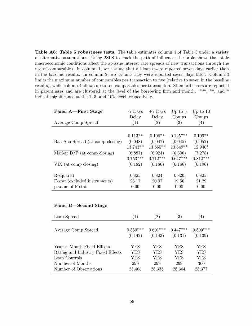
Table A6: Table 5 robustness tests. The table estimates column 4 of Table 5 under a varietyof alternative assumptions. Using 2SLS to track the path of influence, the table shows that stalemacroeconomic conditions affect the at-issue interest rate spreads of new transactions through theuse of comparables. In column 1, we assume that all loans were reported seven days earlier thanin the baseline results. In column 2, we assume they were reported seven days later. Column 3limits the maximum number of comparables per transaction to five (relative to seven in the baselineresults), while column 4 allows up to ten comparables per transaction. Standard errors are reportedin parentheses and are clustered at the level of the borrowing firm and month. ***, **, and *indicate significance at the 1, 5, and 10% level, respectively.

Panel A—First Stage -7 Days +7 Days Up to 5 Up to 10Delay Delay Comps Comps

Average Comp Spread (1) (2) (3) (4)

0.113** 0.106** 0.125*** 0.109**

Baa-Aaa Spread (at comp closing) (0.048) (0.047) (0.045) (0.052)13.743** 13.665** 13.649** 12.940*

Market D/P (at comp closing) (6.887) (6.924) (6.600) (7.278)0.753*** 0.712*** 0.647*** 0.812***

VIX (at comp closing) (0.182) (0.180) (0.166) (0.196)

R-squared 0.825 0.824 0.820 0.825F-stat (excluded instruments) 23.17 20.97 19.50 21.29p-value of F-stat 0.00 0.00 0.00 0.00

Panel B—Second Stage

Loan Spread (1) (2) (3) (4)

Average Comp Spread 0.550*** 0.601*** 0.447*** 0.590***(0.142) (0.143) (0.131) (0.139)

Year × Month Fixed Effects YES YES YES YESRating and Industry Fixed Effects YES YES YES YESLoan Controls YES YES YES YESNumber of Months 299 299 299 300Number of Observations 25,408 25,333 25,364 25,377

59