International Journal "Information Technologies & Knowledge" Vol.5 / 2011

371

COMPARATIVE ANALYSIS FOR ESTIMATING OF THE HURST EXPONET FOR STATIONARY AND NONSTATIONARY TIME SERIES

Ludmila Kirichenko, Tamara Radivilova, Zhanna Deineko

Abstract: Estimating of the Hurst exponent for experimental data plays a very important role in the research of processes which show properties of self-similarity. There are many methods for estimating the Hurst exponent using time series. The aim of this research is to carry out the comparative analysis of the statistical properties of the Hurst exponent estimators obtained by different methods using model stationary and nonstationary fractal time series. In this paper the most commonly used methods for estimating the Hurst exponents are examined. There are: /R S -analysis, variance-time analysis, detrended fluctuation analysis (DFA) and wavelet-based estimation. The fractal Brownian motion that is constructed using biorthogonal wavelets have been chosen as a model random process which exhibit fractal properties. In this paper, the results of a numerical experiment are represented where the fractal Brown motion was modelled for the specified values of the exponent H. The values of the Hurst exponent for the model realizations were varied within the whole interval of possible values 0 < H < 1.The lengths of the realizations were defined as 500, 1000, 2000 and 4000 values. For the nonstationary case model time series are presented by the sum of fractional noise and the trend component, which are a polynomial in varying degrees, irrational, transcendental and periodic functions. The estimates of H were calculated for each generated time series using the methods mentioned above. Samples of the exponent H estimates were obtained for each value of H and their statistical characteristics were researched. The results of the analysis have shown that the estimates of the Hurst exponent, which were obtained for the stationary realisations using the considered methods, are biased normal random variables. For each method the bias depends on the true value of the degrees self-similarity of the process and length of time series. Those estimates which are obtained by the DFA method and the wavelet transformation have the minimal bias. Standard deviations of the estimates depending on the estimation method and decrease, while the length of the series increases. Those estimates which are obtained by using the wavelet analysis have the minimal standard deviation. In the case of a nonstationary time series, represented by a trend and additive fractal noise, more accurate evaluation is obtained using the DFA method. This method allows estimating the Hurst exponent for experimental data with trend components of virtually any kind. The greatest difficulty in estimating, presents a series with a periodic trend component. It is desirable in addition to investigate the spectrum of the wavelet energy, which is demonstrated in the structure of the time series. In the presence of a slight trend, the wavelet-estimation is quite effective. Keywords: Hurst exponent, estimate of the Hurst exponent, self-similar stochastic process, nonstationary time series, methods for estimating the Hurst exponent. ACM Classification Keywords: G.3 Probability and statistics - Time series analysis, Stochastic processes, G.1 Numerical analysis, G.1.2 Approximation - Wavelets and fractals.

International Journal "Information Technologies & Knowledge" Vol.5 / 2011

372

Introduction

Nowadays problems of nonlinear physics, radio electronics, control theory and image processing require the development and employment of new mathematical models, methods and algorithms for data analysis. At present it has been generally accepted, that many stochastic processes in nature and in engineering exhibit a long-range dependence and fractal structure. The most suitable mathematical method for research of the dynamics and structure of such processes is fractal analysis.

The Stochastic process ( )X t is statistically self-similar if the process ( )−Ha X at shows the same second-order

statistical properties as ( )X t . Long-range dependence means slow (hyperbolic) decay in the time of the autocorrelation function of a process. The parameter Н ( < <0 1H ) is called the Hurst exponent and is a measure of self-similarity or a measure of duration of long-range dependence of a stochastic process.

Let us consider the most well-known examples of the self-similar processes. One of the first real stochastic processes, that have been found with self-similar properties is informational data traffic in telecommunication networks. For self-similar traffic methods for calculating the characteristics of a computer network (channel capacity, buffer size, etc.), that is based on classical models, don’t meet the necessary requirements and don’t allow to estimate adequately, the load of the network. There are a large number of publications, which are devoted to the fractal properties analysis and their influence on the functioning and quality of service in the telecommunication network. Another example of fractal stochastic structures is the modern financial market. The modern fractality hypothesis of a financial time series supposes that the market is a self-regulating macro-economic system with feedback which uses information about past events to affect decisions in the present, and contains long-term correlations and trends. The market remains stable, as long as it retains its fractal structure. Analyzing the dynamics of occurrence of time section with various fractal structures, we can diagnose and predict unstable states (crises) of a market. It has become generally accepted in the recent years that a lot of bioelectric signals have fractal structure, so in researches of cerebral and cardio processes are increasingly important roles played by fractal analysis. Distinct changes in fractal characteristics of cardiograms and encephalograms manifest in various diseases, in changes of mental and physical load on the body. Fractal analysis of bioelectrical signals can be the basis for statistical researches, which will allow to formulate a methodology that will be significant for clinical practice.

It is obvious that Hursts’ exponent estimation for experimental data plays an important role in the study of processes which exhibit properties of self-similarity. There are many methods for the Hurst exponent evaluation for a time series. Sufficient review of these methods is represented in [Willinger, 1996; Clegg, 2005]. However, most methods of the Hurst exponent estimation is applied only to stationary time series, while a lot of natural, technical and information processes are nonstationary. The main type of nonstationarity, which occurs in practice, is the existence of trend and cyclical components.

Nevertheless, at the present time there is no proper summary research where the results of the Hurst exponent estimation Í using stationary and nonstationary fractal time series with different methods would be generalized and the comparative analysis of statistical properties of estimations obtained for a small amount of sample data would be. The given research is an attempt to carry out such analysis for the most commonly used methods of estimation of self-similarity.

International Journal "Information Technologies & Knowledge" Vol.5 / 2011

373

The aim of this research is to carry out the comparative analysis of the statistical properties of the Hurst exponent estimates obtained by different methods, using a short length model fractal time series (the number of values being less than 4000). In this paper the most commonly used methods for estimating the Hurst exponent are researched. There are: /R S -analysis (rescaled range method) (see, for instance [Feder, 1988; Peters, 1996; Stollings, 2003; Sheluhin, 2007], variation in time of variance of an aggregate time series (variance-time analysis), see [Stollings, 2003; Sheluhin, 2007], detrended fluctuation analysis (see [Kantelhardt, 2001; Chen, 2002; Gu, 2006; Kantelhardt, 2008]) and estimation using the wavelet analysis (see [Mallat, 1998; Abry, 1998; Abry, 2003]) The fractal Brownian motion has been chosen as a model random process which exhibit fractal properties.

Methods of estimating the Hurst exponent

Rescaled range method. This empirical method suggested by G. Hurst is still one of the most popular methods of research of fractal series of different nature. According to this method for the time series ( )x t of the length τ

the rate ττ( )( )

RS

is defined, where τ( )R is the range of the cumulative deviate series τ( , )cumx t , τ( )S is

standard deviation of the initial series:

( )τ

τ τ

τ =

−=

−− ∑

2

1

max( ( , )) min( ( , ))/1 ( )

1

cum cum

t

x t x tR Sx t x

, τ=1,t , (1)

where τ

ττ =

= ∑1

1( ) ( )t

x x t , τ τ=

= −∑1

( , ) ( ) ( )tcum

ix t x i x .

For a self-similar process and big values of τ this ratio has the following characteristics:

τ ∼ ⋅ ( )HRM c

S, (2)

where c is a constant.

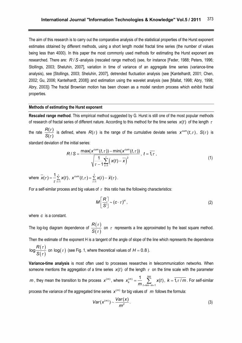
The log-log diagram dependence of ( )( )ττ

RS

on τ represents a line approximated by the least square method.

Then the estimate of the exponent H is a tangent of the angle of slope of the line which represents the dependence ( )( )ττ

logRS

on ( )τlog (see Fig. 1, where theoretical values of = 0.8H ).

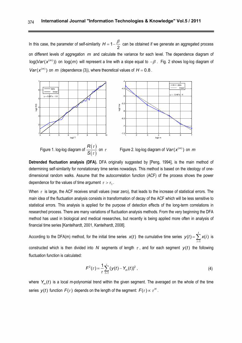
Variance-time analysis is most often used to processes researches in telecommunication networks. When someone mentions the aggregation of a time series ( )x t of the length τ on the time scale with the parameter

m , they mean the transition to the process ( )mx , where = − +

= ∑( )

1

1 ( )km

mk

t km mx x t

m, τ=1, /k m . For self-similar

process the variance of the aggregated time series ( )mx for big values of m follows the formula:

~ β( ) ( )( )m Var xVar x

m. (3)

International Journal "Information Technologies & Knowledge" Vol.5 / 2011

374

In this case, the parameter of self-similarity β= −1

2H can be obtained if we generate an aggregated process

on different levels of aggregation m and calculate the variance for each level. The dependence diagram of ( )log( ( ))mVar x on log( )m will represent a line with a slope equal to β− . Fig. 2 shows log-log diagram of

( )( )mVar x on m (dependence (3)), where theoretical values of = 0.8H .

3 4 5 6 7 8 9 101

2

3

4

5

6

7

log2 T

log2

R/S

y = 0.85*x - 1.6

data linear

1 2 3 4 5 6 7-7.5

-7

-6.5

-6

-5.5

-5

-4.5

-4

log2 m

log2

Var

y = - 0.46*x - 4

data linear

Figure 1. log-log diagram of ( )( )ττ

RS

on τ Figure 2. log-log diagram of ( )( )mVar x on m

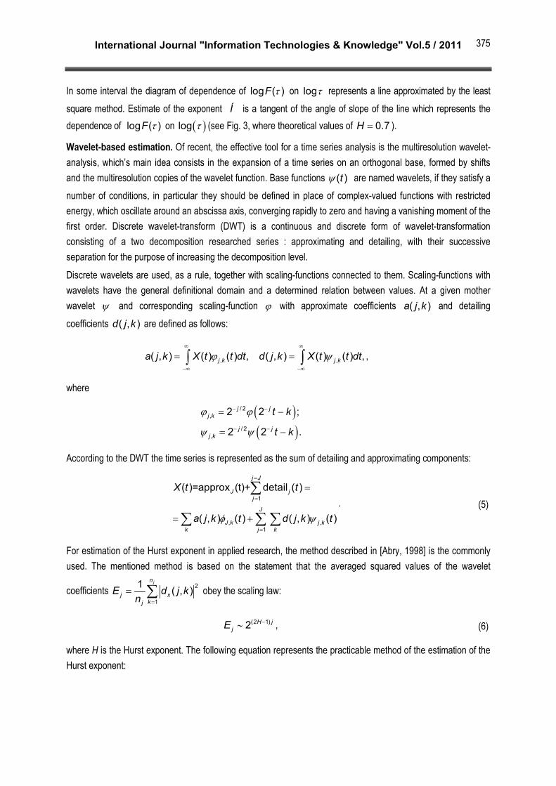
Detrended fluctuation analysis (DFA). DFA originally suggested by [Peng, 1994], is the main method of determining self-similarity for nonstationary time series nowadays. This method is based on the ideology of one-dimensional random walks. Assume that the autocorrelation function (ACF) of the process shows the power dependence for the values of time argument τ τ> 1 .

When τ is large, the ACF receives small values (near zero), that leads to the increase of statistical errors. The main idea of the fluctuation analysis consists in transformation of decay of the ACF which will be less sensitive to statistical errors. This analysis is applied for the purpose of detection effects of the long-term correlations in researched process. There are many variations of fluctuation analysis methods. From the very beginning the DFA method has used in biological and medical researches, but recently is being applied more often in analysis of financial time series [Kantelhardt, 2001, Kantelhardt, 2008].

According to the DFA(m) method, for the initial time series ( )x t the cumulative time series =

= ∑1

( ) ( )t

iy t x i is

constructed which is then divided into N segments of length τ , and for each segment ( )y t the following fluctuation function is calculated:

τ

ττ =

= −∑2 2

1

1( ) ( ( ) ( ))mt

F y t Y t , (4)

where ( )mY t is a local m-polynomial trend within the given segment. The averaged on the whole of the time

series ( )y t function τ( )F depends on the length of the segment: τ τ∝( ) HF .

International Journal "Information Technologies & Knowledge" Vol.5 / 2011

375

In some interval the diagram of dependence of τlog ( )F on τlog represents a line approximated by the least square method. Estimate of the exponent Í is a tangent of the angle of slope of the line which represents the dependence of τlog ( )F on ( )τlog (see Fig. 3, where theoretical values of = 0.7H ).

Wavelet-based estimation. Of recent, the effective tool for a time series analysis is the multiresolution wavelet-analysis, which’s main idea consists in the expansion of a time series on an orthogonal base, formed by shifts and the multiresolution copies of the wavelet function. Base functions ψ ( )t are named wavelets, if they satisfy a number of conditions, in particular they should be defined in place of complex-valued functions with restricted energy, which oscillate around an abscissa axis, converging rapidly to zero and having a vanishing moment of the first order. Discrete wavelet-transform (DWT) is a continuous and discrete form of wavelet-transformation consisting of a two decomposition researched series : approximating and detailing, with their successive separation for the purpose of increasing the decomposition level.

Discrete wavelets are used, as a rule, together with scaling-functions connected to them. Scaling-functions with wavelets have the general definitional domain and a determined relation between values. At a given mother wavelet ψ and corresponding scaling-function ϕ with approximate coefficients ( , )a j k and detailing coefficients ( , )d j k are defined as follows:

ϕ ψ∞ ∞

−∞ −∞

= =∫ ∫, ,( , ) ( ) ( ) , ( , ) ( ) ( ) ,j k j ka j k X t t dt d j k X t t dt ,

where

( )( )

ϕ ϕ

ψ ψ

− −

− −

= −

= −

/ 2,

/ 2,

2 2 ;

2 2 .

j jj k

j jj k

t k

t k

According to the DWT the time series is represented as the sum of detailing and approximating components:

φ ψ

=

=

=

=

= +

∑

∑ ∑ ∑

1

, ,1

( )=approx (t)+ detail ( )

( , ) ( ) ( , ) ( )

j J

J jj

J

J k j kk j k

X t t

a j k t d j k t. (5)

For estimation of the Hurst exponent in applied research, the method described in [Abry, 1998] is the commonly used. The mentioned method is based on the statement that the averaged squared values of the wavelet

coefficients =

= ∑ 2

1

1 ( , )jn

j xkj

E d j kn

obey the scaling law:

−∼ (2 1)2 H jjE , (6)

where H is the Hurst exponent. The following equation represents the practicable method of the estimation of the Hurst exponent:

International Journal "Information Technologies & Knowledge" Vol.5 / 2011

376

=

= − +

∑

22 2

1

1log log ( , ) (2 1)jn

jkj

E d j k H j constn

. (7)

From this formula it can be concluded that if there is the long-range dependence of the time series ( )x t then the

Hurst exponent H can be obtained by estimating the slope of the graph of the function 2log ( )jE from j . Fig. 4

shows dependence 2log ( )jE on j (dependence 7), where theoretical values of = 0.7H .

Modelling of fractal Brownian motion

One of the well known and simple models of stochastic dynamics which exhibits fractal properties is fractal Brownian motion (fBm). It is widely used in physics, chemistry, biology, economics and theory of network traffic.

Gaussian process ( )X t is called fractal Brownian motion with the parameter < <, 0 1H H , if the increments of the random process τ τ∆ = + −( ) ( ) ( )X X t X t are distributed in the following way

σ τπσ τ −∞

∆ < = ⋅ −

∫

2

2 200

1( ) Exp22

x

HH

zP X x dz , (8)

where σ0 is diffusion coefficient.

4 4.5 5 5.5 6 6.5

-1.8

-1.6

-1.4

-1.2

-1

-0.8

-0.6

-0.4

-0.2

0

0.2

log2 T

log2

F

y = 0.69*x - 4.4

data linear

1 2 3 4 5 6 7 8 9 10-6

-5

-4

-3

-2

-1

0

1

2

3

j

log2

Ej

y = 0.71*x - 5.7

data linear

Figure 3. log-log diagram of τ( )F on τ Figure 4. Dependence 2log ( )jE on j

fBm with the parameter = 0.5H coincides with the classic Brownian motion. Increments of fBm are called fractal Gaussian noise and its dispersion can be described by the formula τ σ τ+ − = 2 2

0[ ( ) ( )] HD X t X t .

There are many methods of construction of fBm for the case of discrete time, which have been considered in [Mandelbrot, 1983; Feder, 1988; Voss, 1988; Cronover, 2000]. These models have some weak sides. One of them is underestimating/overestimating of the degree of self-similarity of a process for small and big theoretical values of the Hurst exponent and the short length of a model realisation [Jeongy, 1998; Cronover, 2000; Sheluhin, 2007].

One of the methods which can help to resolve the mentioned problems is the construction of fBm using biorthogonal wavelets [Sellan, 1995; Abry, 1996; Sellan, 1995; Meyer, 1999; Bardet, 2003]. In this case the fBm

International Journal "Information Technologies & Knowledge" Vol.5 / 2011

377

realization is constructed using discrete wavelet transform where the detail wavelet coefficients on each level are independent normal random values and approximation wavelet coefficients are obtained using fractal autoregression and moving average process FARIMA:

ε∞ ∞ ∞

−

=−∞ = =−∞

= Φ − + Ψ − −∑ ∑ ∑( ), 0

0( ) ( ) 2 (2 )H jH j

H H k H j kk j k

B t t k S t k b , (9)

where ΨH is biorthogonal base wavelet function, ΦH is corresponding ΨH scaling function, ( )HkS is stationary

Gaussian process FARIMA with the fractal differentiation parameter = − 0.5d H , ε ,j k – independent standard

Gaussian random values, 0b – constant where =(0) 0HB .

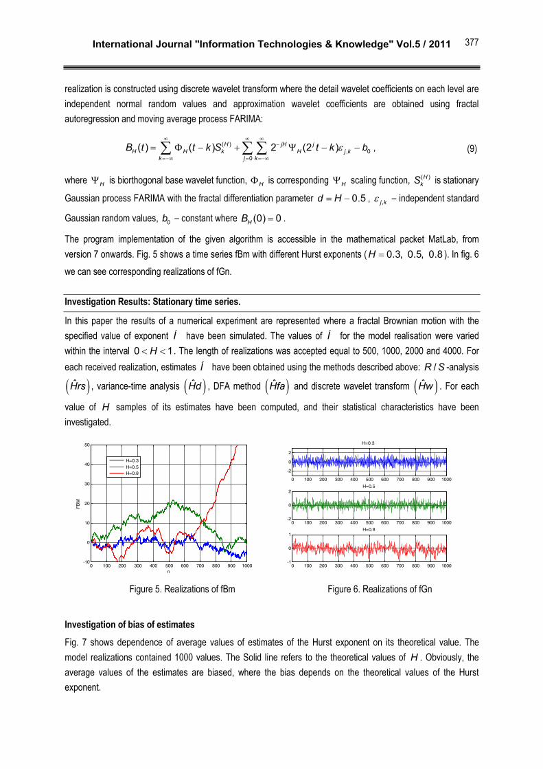
The program implementation of the given algorithm is accessible in the mathematical packet MatLab, from version 7 onwards. Fig. 5 shows a time series fBm with different Hurst exponents ( = 0.3, 0.5, 0.8H ). In fig. 6 we can see corresponding realizations of fGn.

Investigation Results: Stationary time series.

In this paper the results of a numerical experiment are represented where a fractal Brownian motion with the specified value of exponent Í have been simulated. The values of Í for the model realisation were varied within the interval < <0 1H . The length of realizations was accepted equal to 500, 1000, 2000 and 4000. For each received realization, estimates Í have been obtained using the methods described above: /R S -analysis

( )Hrs , variance-time analysis ( )Hd , DFA method ( )Hfa and discrete wavelet transform ( )Hw . For each

value of H samples of its estimates have been computed, and their statistical characteristics have been investigated.

0 100 200 300 400 500 600 700 800 900 1000-10

0

10

20

30

40

50

n

FBM

H=0.3H=0.5H=0.8

0 100 200 300 400 500 600 700 800 900 1000

-2

0

2

H=0.3

0 100 200 300 400 500 600 700 800 900 1000-2

0

2H=0.5

0 100 200 300 400 500 600 700 800 900 1000-1

0

1H=0.8

Figure 5. Realizations of fBm Figure 6. Realizations of fGn

Investigation of bias of estimates Fig. 7 shows dependence of average values of estimates of the Hurst exponent on its theoretical value. The model realizations contained 1000 values. The Solid line refers to the theoretical values of H . Obviously, the average values of the estimates are biased, where the bias depends on the theoretical values of the Hurst exponent.

International Journal "Information Technologies & Knowledge" Vol.5 / 2011

378

Obviously, the estimates of the Hurst exponent are biased in a region of persistence as well as in an antipersistence one. Since most of the fractal processes have a long-range dependence, we will be considering results only for the interval < <0,5 1H . From Fig. 7 we can see that the estimates obtained by the methods of

/R S - analysis and variance-time analysis are the most biased.

Let us consider the results of estimation of the exponent H by the method of /R S -analysis. The method of the rescaled range proposed by Hurst is, perhaps, the most popular one and is used in all fields of scientific research. Its main merit is its robustness. Actually, this method works even on non-stationary data. But also, as it was noticed by Hurst, the estimates of H below ≈ 0,75H obtained by the /R S -method are overestimated, and the estimate of H over ≈ 0,75H are understate.

Fig. 8 represents a dependence of average values of estimates Hrs on theoretical values of H for model series of different length. Obviously, the average values of estimates can be approximates quite well with lines

= +ˆN N NH k H b , where coefficients Nk and Nb depend on the realization N where the estimation is done.

This lines cross the line of the theoretical values of H at around ≈ 0,75H ; and are overestimated below this values and are underestimated above this value. The results of the performed research confirm the results obtained by analysing the estimation of other models [Feder, 1988; Jeongy, 1998; Кириченко, 2005; Sheluhin, 2007]. With the increase of the realisation length N the angle of slope Nk of the approximated line increases slowly and approaches the theoretical value π / 4 .

0.1 0.2 0.3 0.4 0.5 0.6 0.7 0.8 0.90.1

0.2

0.3

0.4

0.5

0.6

0.7

0.8

0.9

Theoretical H

Est

imat

e H

HHwHrsHdHfa

Figure 7. Dependence of the average values of estimates obtained by various methods on the theoretical H

Due to its simplicity and easy understanding of its results the method of variance-time analysis is the most commonly used for assessment of self-similarity of the information network traffic. Nevertheless, for processes with a long-range dependence, this method gives undervalued estimates. [Jeongy, 1998; Кириченко, 2005; Sheluhin, 2007]. This can be unacceptable, for instance, in the case of assessment of the network load during the transmission of the self-similar traffic. [Stollings, 2003].

International Journal "Information Technologies & Knowledge" Vol.5 / 2011

379

0.5 0.55 0.6 0.65 0.7 0.75 0.8 0.85 0.9 0.95 10.5

0.55

0.6

0.65

0.7

0.75

0.8

0.85

0.9

0.95

1

Theoretical H

Est

imat

e H

H500100020004000

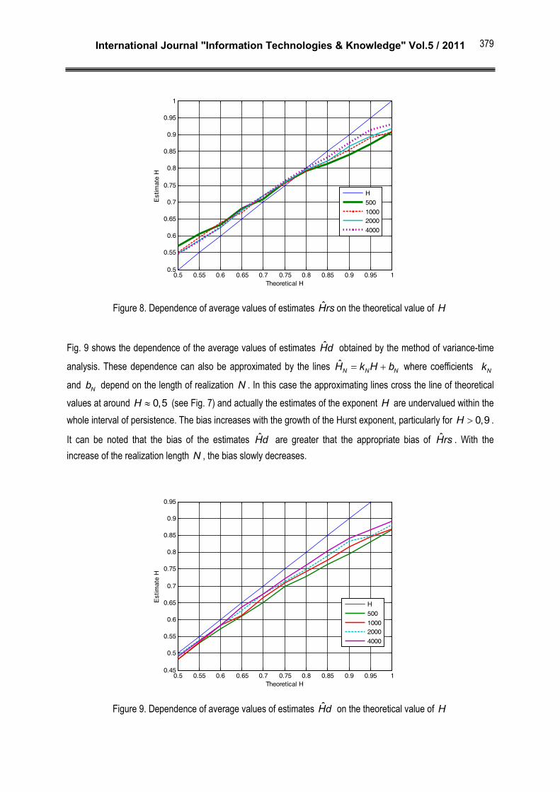
Figure 8. Dependence of average values of estimates Hrs on the theoretical value of H

Fig. 9 shows the dependence of the average values of estimates Hd obtained by the method of variance-time

analysis. These dependence can also be approximated by the lines = +ˆN N NH k H b where coefficients Nk

and Nb depend on the length of realization N . In this case the approximating lines cross the line of theoretical values at around ≈ 0,5H (see Fig. 7) and actually the estimates of the exponent H are undervalued within the whole interval of persistence. The bias increases with the growth of the Hurst exponent, particularly for > 0,9H .

It can be noted that the bias of the estimates Hd are greater that the appropriate bias of Hrs . With the increase of the realization length N , the bias slowly decreases.

0.5 0.55 0.6 0.65 0.7 0.75 0.8 0.85 0.9 0.95 10.45

0.5

0.55

0.6

0.65

0.7

0.75

0.8

0.85

0.9

0.95

Theoretical H

Est

imat

e H

H500100020004000

Figure 9. Dependence of average values of estimates Hd on the theoretical value of H

International Journal "Information Technologies & Knowledge" Vol.5 / 2011

380

The DFA method is based on the ideology of one-dimensional random walk and is widely used in the analysis of bioelectric signals. The estimates Hfa obtained by the DFA method can be characterised by a small bias within the interval < <0,5 0,9H (see Fig. 10) even for realizations of short length. The sign of this bias reverses and increases for > 0,9H . It should be brought into focus that most of the natural and information fractal processes have a degree of self-similarity less than 0,9.

0.5 0.55 0.6 0.65 0.7 0.75 0.8 0.85 0.9 0.95 10.5

0.55

0.6

0.65

0.7

0.75

0.8

0.85

0.9

0.95

1

Theoretical H

Est

imat

e H

H500100020004000

Figure 10. Dependence of the average values of the estimates Hfa on the theoretical value of H

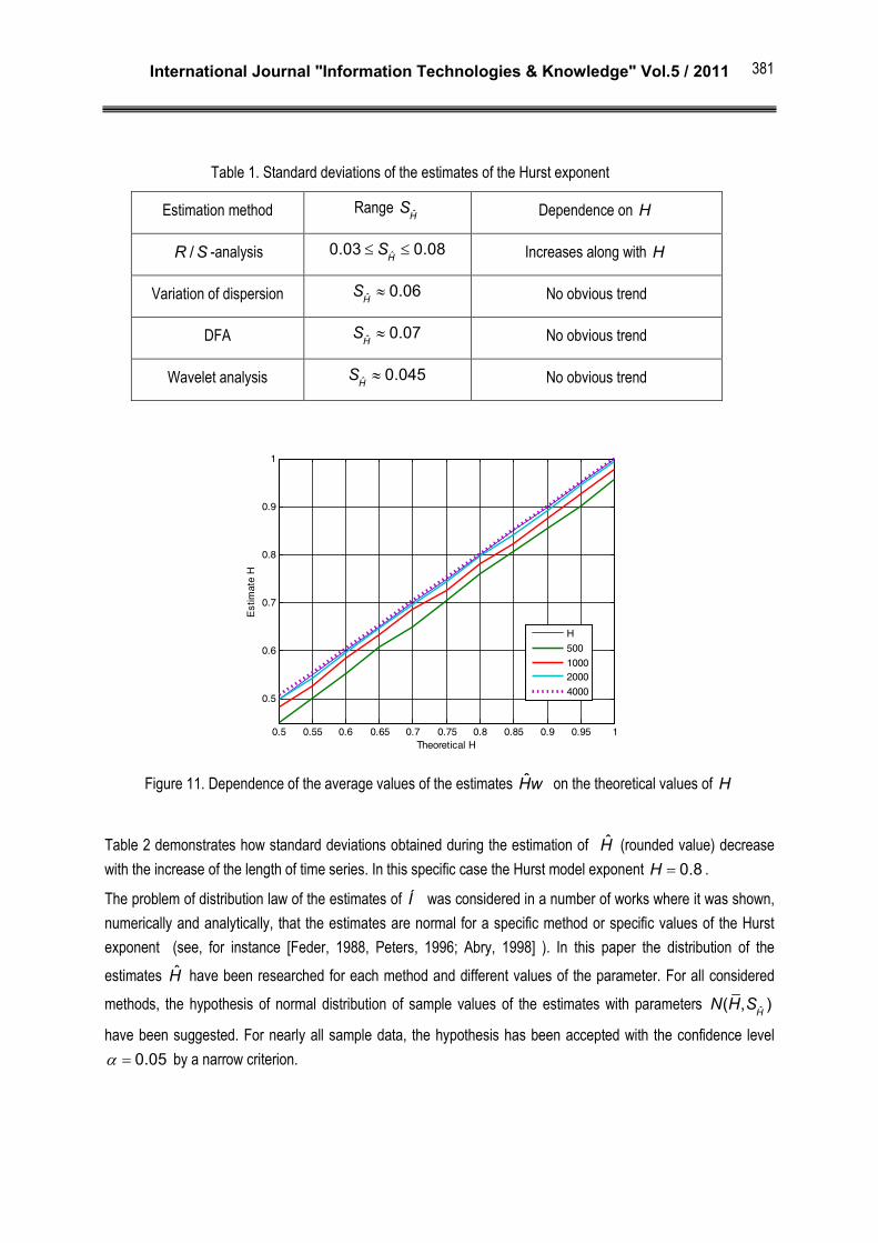
The methods of estimation of the Hurst exponent by the use of wavelet analysis are the most recent and still have not been commonly used. Nevertheless, their merits are obvious. In the paper [Abry, 1998] it has been shown that the estimates are asymptotically unbiased if base wavelets are chosen in a proper way. Fig 11 represents the dependence of the average values of Hw obtained by the method of discrete wavelet expansion with the base wavelet function of Daubechies D4. It is obvious that with the increase of the time series length N the bias decreases and is actually equal to 0 for ≈ 4000N .

Research of the standard deviations of the estimates In this paper, the dependence of standard deviations of estimates of the Hurst exponent on the values of H and length of the model fractal series has been investigated for each method. In Table 1 the values of the standard deviations of the estimates of the Hurst exponent which have been received for the series of length for 1000 values are represented.

International Journal "Information Technologies & Knowledge" Vol.5 / 2011

381

Table 1. Standard deviations of the estimates of the Hurst exponent

Estimation method Range H

S Dependence on H

/R S -analysis ≤ ≤ˆ0.03 0.08H

S Increases along with H

Variation of dispersion ≈ˆ 0.06H

S No obvious trend

DFA ≈ˆ 0.07H

S No obvious trend

Wavelet analysis ≈ˆ 0.045H

S No obvious trend

0.5 0.55 0.6 0.65 0.7 0.75 0.8 0.85 0.9 0.95 1

0.5

0.6

0.7

0.8

0.9

1

Theoretical H

Est

imat

e H

H500100020004000

Figure 11. Dependence of the average values of the estimates Hw on the theoretical values of H

Table 2 demonstrates how standard deviations obtained during the estimation of H (rounded value) decrease with the increase of the length of time series. In this specific case the Hurst model exponent = 0.8H .

The problem of distribution law of the estimates of Í was considered in a number of works where it was shown, numerically and analytically, that the estimates are normal for a specific method or specific values of the Hurst exponent (see, for instance [Feder, 1988, Peters, 1996; Abry, 1998] ). In this paper the distribution of the estimates H have been researched for each method and different values of the parameter. For all considered methods, the hypothesis of normal distribution of sample values of the estimates with parameters ˆ( , )

HN H S

have been suggested. For nearly all sample data, the hypothesis has been accepted with the confidence level α = 0.05 by a narrow criterion.

International Journal "Information Technologies & Knowledge" Vol.5 / 2011

382

Table 2. Standard deviations of the estimates depending on length of time series

HS 500 1000 2000 4000

HrsS 0.08 0.06 0.05 0.04

HdS 0.07 0.06 0.05 0.045

HfaS 0.085 0.07 0.055 0.045

HwS 0.065 0.045 0.03 0.02

Thus, the estimates of the Hurst exponent which are obtained by the methods considered above are biased normal random variables. For each method, the bias depends on a true value of degree of self-similarity and the length of a time series. Standard deviations of the estimates depend on the estimation method and decrease with the growth of the series length.

Research results: nonstationary time series

We investigated different model time series, presented by the sum of fractional Brownian noise the specified value of the Hurst exponent and the trend component, which is a polynomial in varying degrees, irrational, transcendental and periodic functions ( see Fig. 12). The total signal can be written as

= +( ) * ( ) ( )Y t k T t fgn t ,

where ( )T t is a trend, ( )fgn t is a fractal Gaussian noise, and k a is a factor that regulates the ratio of trend to the noise.

Figure 12. Model nonstationary time series

Detrended fluctuation analysis. The DFA(m) method is traditionally used in analyzing the fractal structure and estimating the degree of self-similarity of a time series with trends (for example, the implementation of encephalograms) or cumulative series with nonstationary increments (for example, financial series).

In this paper, in each case in the construction of the fluctuation functions, a local polynomial trend of increasing orders was considered [Kirichenko, 2010].The numerical study of a fractal series with a polynomial trend

International Journal "Information Technologies & Knowledge" Vol.5 / 2011

383

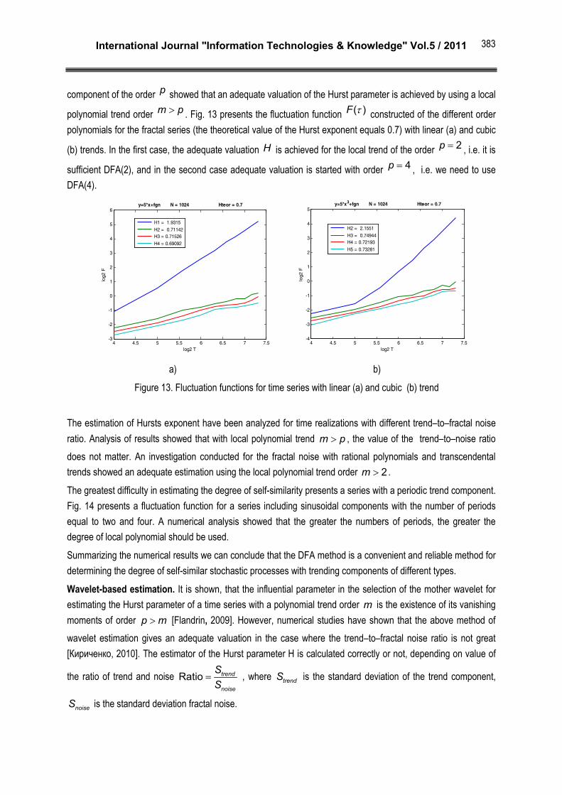
component of the order p showed that an adequate valuation of the Hurst parameter is achieved by using a local

polynomial trend order >m p . Fig. 13 presents the fluctuation function τ( )F constructed of the different order polynomials for the fractal series (the theoretical value of the Hurst exponent equals 0.7) with linear (a) and cubic

(b) trends. In the first case, the adequate valuation H is achieved for the local trend of the order = 2p , i.e. it is

sufficient DFA(2), and in the second case adequate valuation is started with order = 4p , i.e. we need to use DFA(4).

4 4.5 5 5.5 6 6.5 7 7.5-3

-2

-1

0

1

2

3

4

5

6

log2 T

log2

F

y=5*x+fgn N = 1024 Hteor = 0.7

H1 = 1.9315 H2 = 0.71142 H3 = 0.71526 H4 = 0.69092

4 4.5 5 5.5 6 6.5 7 7.5-4

-3

-2

-1

0

1

2

3

4

5

log2 T

log2

F

y=5*x3+fgn N = 1024 Hteor = 0.7

H2 = 2.1551 H3 = 0.74944 H4 = 0.72193 H5 = 0.73281

a) b)

Figure 13. Fluctuation functions for time series with linear (a) and cubic (b) trend

The estimation of Hursts exponent have been analyzed for time realizations with different trend–to–fractal noise ratio. Analysis of results showed that with local polynomial trend >m p , the value of the trend–to–noise ratio does not matter. An investigation conducted for the fractal noise with rational polynomials and transcendental trends showed an adequate estimation using the local polynomial trend order > 2m .

The greatest difficulty in estimating the degree of self-similarity presents a series with a periodic trend component. Fig. 14 presents a fluctuation function for a series including sinusoidal components with the number of periods equal to two and four. A numerical analysis showed that the greater the numbers of periods, the greater the degree of local polynomial should be used.

Summarizing the numerical results we can conclude that the DFA method is a convenient and reliable method for determining the degree of self-similar stochastic processes with trending components of different types.

Wavelet-based estimation. It is shown, that the influential parameter in the selection of the mother wavelet for estimating the Hurst parameter of a time series with a polynomial trend order m is the existence of its vanishing moments of order >p m [Flandrin, 2009]. However, numerical studies have shown that the above method of wavelet estimation gives an adequate valuation in the case where the trend–to–fractal noise ratio is not great [Кириченко, 2010]. The estimator of the Hurst parameter H is calculated correctly or not, depending on value of

the ratio of trend and noise =Ratio trend

noise

SS

, where trendS is the standard deviation of the trend component,

noiseS is the standard deviation fractal noise.

International Journal "Information Technologies & Knowledge" Vol.5 / 2011

384

0 100 200 300 400 500 600 700 800 900 1000-1.5

-1

-0.5

0

0.5

1

1.5

0 100 200 300 400 500 600 700 800 900 1000-1.5

-1

-0.5

0

0.5

1

1.5

4 4.5 5 5.5 6 6.5 7 7.5-3

-2

-1

0

1

2

3

4

5

6

log2 T

log2

F

y=sin x +fgn N = 1024 Hteor = 0.7

H2 = 2.4798 H3 = 1.4798 H4 = 0.71598 H5 = 0.63037

4 4.5 5 5.5 6 6.5 7 7.5-3

-2

-1

0

1

2

3

4

5

log2 T

log2

F

y=sin x +fgn N = 1024 Hteor = 0.7

H2 = 2.202 H3 = 1.3815 H4 = 0.88314 H5 = 0.68364

Figure 14. Model time series with sinusoidal trends and corresponding fluctuation functions for DFA(2)- DFA(5)

The numerical investigation have shown that the value *Ratio , from which the effect of trend becomes significant, does not depend on the length of the model realization, but only on the standard deviation of the fractal process and factor k in the expression * ( )k T t . The table 3 shows the experimental results for various

model signals and the value of *Ratio .

Table 3. Model trends and the value of *Ratio

Trend Value of

Ratio*

Trend Value of

Ratio*

T(t) = k∙t 9 = ⋅34( )T t k t 0,45

T(t) = k∙t2 7 T(t) = k∙ln(t) 0,30

T(t) = k∙t3 5

T(t) = k

sin(2πt),

1 period

0,18

T(t) = k∙√t 2

T(t) =

k∙sin(2πt),

2 periods

0,08

To understand why the trend component leads to a deterioration of estimation, let us consider in more detail the spectrum of the wavelet energy of the signal jE , which obeys the scaling law −∼ (2 1)2 H j

jE . The wavelet energy

is equal to the amount of energy at a given level of wavelet decomposition =

= ∑ 2

1

1 d( , )jN

jkj

E j kN

. The Fig. 15

International Journal "Information Technologies & Knowledge" Vol.5 / 2011

385

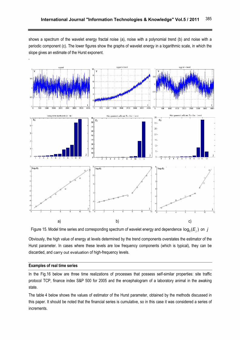
shows a spectrum of the wavelet energy fractal noise (a), noise with a polynomial trend (b) and noise with a periodic component (c). The lower figures show the graphs of wavelet energy in a logarithmic scale, in which the slope gives an estimate of the Hurst exponent.

‘

a) b) c)

Figure 15. Model time series and corresponding spectrum of wavelet energy and dependence 2log ( )jE on j

Obviously, the high value of energy at levels determined by the trend components overstates the estimator of the Hurst parameter. In cases where these levels are low frequency components (which is typical), they can be discarded, and carry out evaluation of high-frequency levels.

Examples of real time series

In the Fig.16 below are three time realizations of processes that possess self-similar properties: site traffic protocol TCP, finance index S&P 500 for 2005 and the encephalogram of a laboratory animal in the awaking state.

The table 4 below shows the values of estimator of the Hurst parameter, obtained by the methods discussed in this paper. It should be noted that the financial series is cumulative, so in this case it was considered a series of increments.

International Journal "Information Technologies & Knowledge" Vol.5 / 2011

386

Conclusion

Thus, the estimates of the Hurst exponent which are obtained for the stationary realisations by the methods considered above are biased normal random variables. For each method the bias depends on a true value of the degree of self-similarity and the length of a time series. Standard deviations of the estimates depend on the estimation method and decrease with the growth of the series length.

Table 4. Estimates of the Hurst exponent Method /R S -analysis Variance-analysis DFA(1) Wavelet- estimation

Traffic

(N=2000) = =ˆ 0.69; 0.05H S

= =ˆ 0.81; 0.05H S

= =ˆ 0.75; 0.055H S

= =ˆ 0.78; 0.03H S

Index S&P 500

(N=250) = =ˆ 0.65; 0.09H S

= =ˆ 0.51; 0.08H S

= =ˆ 0.57; 0.09H S

= =ˆ 0.6; 0.07H S

Encephalogram

(N=1000) = =ˆ 0.72; 0.06H S

= =ˆ 0.63; 0.06H S

= =ˆ 0.68; 0.07H S

= =ˆ 0.65; 0.045H S

0 200 400 600 800 1000 1200 1400 1600 1800 20000

0.5

1

1.5

2

2.5

3

3.5

4

4.5x 10

4

0 50 100 150 200 25060

65

70

75

80

85

90

95

0 100 200 300 400 500 600 700 800 900 1000

-6

-4

-2

0

2

4

6

8

a) b) c)

Figure 16. Time series of traffic protocol TCP, finance index and encephalogram

Summarizing the results of the numerical research we can make a conclusion that the estimates with the least bias and standard deviation can be given by the method which uses wavelet analysis. Also, other methods have some merits which can be significant in relation to some aims and ways of the research. For instance, /R S -analysis allows to estimate the degree of self- similarity of a time series for which the wavelet estimation nearly cannot be applied, The DFA method gives the best results for short series. Thus, in most cases for the estimation of the Hurst exponent it makes sense to use various methods and comparison of the results provides extra information.

In the case of a nonstationary time series represented, a trend and additive fractal noise, more accurate evaluation is obtained using the DFA method. This method allows estimation of the Hurst exponent for experimental data with trend components of virtually any kind. The greatest difficulty in estimating presents a series with a periodic trend component. It is desirable in addition to investigate the spectrum of the wavelet energy, which is demonstrates the structure of the time series. It should be noted that in the presence of a slight trend, the wavelet-estimation is quite effective.

International Journal "Information Technologies & Knowledge" Vol.5 / 2011

387

Bibliography

[Abry, 1996] P. Abry. The wavelet-based synthesis for the fractional Brownian motion proposed by F. Sellan and Y. Meyer. Remarks and fast implementation. Р. Abry, F. Sellan. Applications and Computering Harmonic Analise (V.3(4)), 1996.

[Abry, 1998] P. Abry. Wavelet analysis of long-range dependent traffic. P. Abry, D. Veitch. IEEE/ACM Transactions Information Theory (№ 1(44), 1998.

[Abry, 2003] P. Abry. Self-similarity and long-range dependence through the wavelet lens. Р. Abry, P. Flandrin, M.S. Taqqu, D. Veitch. Theory and applications of long-range dependence, Birkhäuser, 2003.

[Bardet, 2003] J.-M. Bardet. Generators of long-range dependence processes: a survey, Theory and applications of long-range dependence. Bardet J.-M., G. Lang, G. Oppenheim, A. Philippe, S. Stoev, M.S. Taqqu. Theory and applications of long-range dependence, Birkhäuser, 2003.

[Chen, 2002] Z. Chen. Effect of non-stationaritieson detrended fluctuation analysis. Z. Chen, P.Ch. Ivanov, K. Hu, H.E. Stanley. Phys. Rev. E 65, 041107, 2002.

[Clegg, 2005] R.G. Clegg. A practical guide to measuring the Hurst parameter. R. G. Clegg. Computing science technical report (№ CS–TR–916), 2005.

[Cronover, 2000] R. M. Cronover. Introduction to fractals and chaos. R. M. Cronover. John and Bartlett Publishers, N.Y., 2000.

[Feder, 1988] J. Feder. Fractals. J. Feder. Plenum, New York, 1988. [Flandrin, 2009] Patrick Flandrin. Scale Invariance and Wavelets. Patrick Flandrin, Paulo Gonзalves and Patrice

Abry in Scaling, Fractals and Wavelets. Ed. by P. Abry, P. Gonçalves, J. Lévy Véhel. John Wiley & Sons, London, 2009.

[Gu, 2006] G.-F. Gu. Detrended fluctuation analysis for fractals and multifractals in higher dimensions. G.-F. Gu, W.-X. Zhou. Phys. Rev. (E 74, 061104), 2006.

[Jeongy, 1998] H.-D. J. Jeongy. A Comparative Study of Generators of Synthetic Self-Similar Teletrafic. H.-D. J. Jeongy, McNickle D., Pawlikowski K. Department of Computer Science and Management, University of Canterbury, 1998.

[Kantelhardt, 2001] J.W. Kantelhardt. Detecting long-range correlations with detrended fluctuation analysis. J.W. Kantelhardt, E. Koscielny-Bunde, H.H.A. Rego, S. Havlin, A. Bunde. Phys (A 295, 441), 2001.

[Kantelhardt, 2008] J. W. Kantelhardt. Fractal and Multifractal Time Series. J. W. Kantelhardt. http://arxiv.org/abs/0804.0747, 2008.

[Kirichenko, 2010] L. Kirichenko. Application of DFA method in fractal analysis of time series of different nature L. Kirichenko,Т.Radivilova, Zh. Deineko .Abstracts of International Conference Modern Stochastics: Theory and Application II, Kyiv, 2010.

[Mallat, 1998] S. Mallat. A wavelet tour of signal processing. S. Mallat. Academic Press, San Diego, London, Boston, N.Y., Sydney, Tokyo, Toronto, 1998.

[Mandelbrot, 1983] B. B. Mandelbrot. The Fractal Geometry of Nature. B. B. Mandelbrot. W.H. Freeman, San Francisco, 3rd Edition, 1983.

[Meyer, 1999] Y. Meyer. Wavelets, generalized white noise and fractional integration: the synthesis of fractional Brownian motion. Y. Meyer, F. Sellan, M.S. Taqqu. The Journal of Fourier Analysis and Applications 5(5), Birkhäuser, Boston1999.

[Peng, 1994] C.-K. Peng. Mosaic organization of DNA nucleotides. C.-K. Peng, S.V. Buldyrev, S. Havlin, M. Simons, H.E. Stanley, A.L. Goldberger. Phys. Rev. (E 49, 1685),1994.

[Peters, 1996] Edgar E. Peters. Chaos and Order in the Capital Markets: A New View of Cycles, Prices, and Market Volatility. Edgar E. Peters. Wiley, 2 edition, 1996.

International Journal "Information Technologies & Knowledge" Vol.5 / 2011

388

[Sellan, 1995] F. Sellan. Synthµese de mouvements browniens fractionnaires µa l'aide de la transformation par ondelettes. F. Sellan. Comptes Rendus de l'Academie des Sciences de Paris, Serie I, 1995.

[Sheluhin, 2007] Oleg I. Sheluhin. Self-similar processes in telecommunications. Oleg I. Sheluhin, Sergey M. Smolskiy, Andrey V. Osin. JohnWiley & Sons Ltd, Chichester, 2007.

[Stollings, 2003] W. Stollings. High-speed networks and Internets. Performance and quality of service. W. Stollings. New Jersey, 2002.

[Voss, 1988] R. F Voss. Fractals in nature: From characterization to simulation in The Science of Fractal Images. R. F Voss. Springer-Verlag, New York, 1988.

[Willinger, 1996] W. Willinger. Bibliographical guide to self-similar traffic and performance modeling for modern high-speed network in «Stohastic networks: theory and applications». W. Willinger, M. S. Taqqu, A. A. Erramilli. Claredon Press (Oxford University Press), Oxford, 1996.

[Кириченко, 2005] Л. О Кириченко. Cравнительный анализ методов оценки параметра Xерста самоподобных процессов Л. О. Кириченко, Т. А. Радивилова, М. И. Синельникова. Системи обробки інформації Вип. 8(48), Харьков, 2005.

[Кириченко, 2010] Л. О Кириченко. Оценивание параметра Хёрста для временных рядов с трендом методом вейвлет-преобразования. Л. О Кириченко, Ж.В. Дейнеко. Системи управління навігації та зв’язку. Вип 4 (16), Київ, 2010.

Authors' Information

Ludmila Kirichenko – Ph. D., Associate professor, Kharkiv National University of Radio Electronics; 14 Lenin Ave., 61166 Kharkiv, Ukraine; e-mail: ludmila.kirichenko@gmail.com.

Major Fields of Scientific Research: Time series analysis, Stochastic self-similar processes, Wavelets , Fractals, Chaotic systems

Tamara Radivilova – Ph. D., Associate professor, Kharkiv National University of Radio Electronics; 14 Lenin Ave., 61166 Kharkiv, Ukraine; e-mail: tomachka_7@yahoo.com.

Major Fields of Scientific Research: Wavelets and fractals, Computer systems and networks

Zhanna Deineko - lecturer, Kharkiv National University of Radio Electronics; 14 Lenin Ave., 61166 Kharkiv, Ukraine; e-mail: shanna@kture.kharkov.ua.

Major Fields of Scientific Research: Wavelets and fractals