Embed Size (px)
Citation preview

Comparative analysis of SWAT model with Coupled SWAT-MODFLOW model for Gibbs Farm Watershed in
Georgia
Presented By K.Sangeetha
B.Narasimhan D.D.Bosch A.W.Coffin
1 2018 SWAT INTERNATIONAL CONFERENCE, JAN 10-12, CHENNAI

Outline of the Study
Motivation
Study Area Description – Gibbs farm watershed
Methodology
Model setup
Results and Discussions
Conclusion
Future Work
2
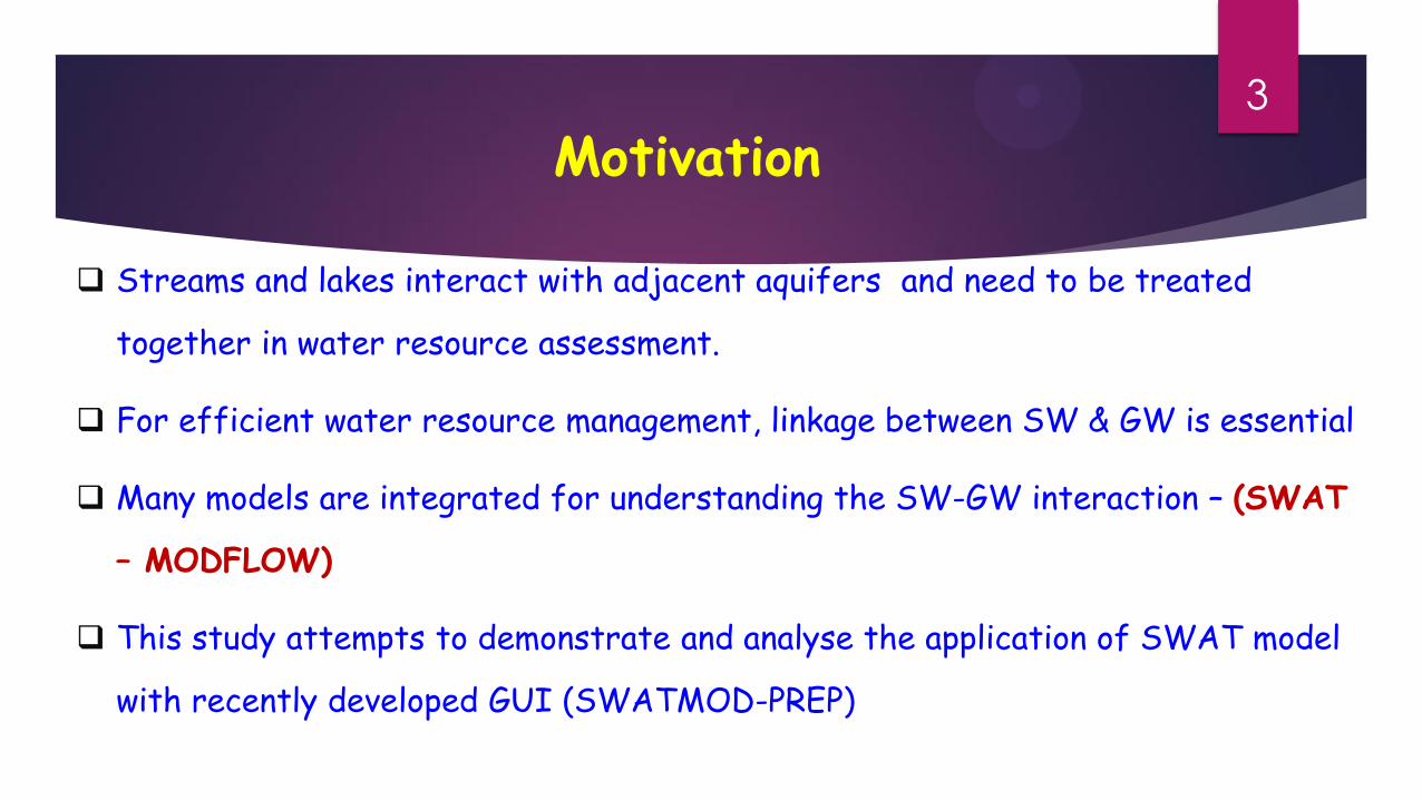
Motivation
Streams and lakes interact with adjacent aquifers and need to be treated
together in water resource assessment.
For efficient water resource management, linkage between SW & GW is essential
Many models are integrated for understanding the SW-GW interaction – (SWAT
– MODFLOW)
This study attempts to demonstrate and analyse the application of SWAT model
with recently developed GUI (SWATMOD-PREP)
3
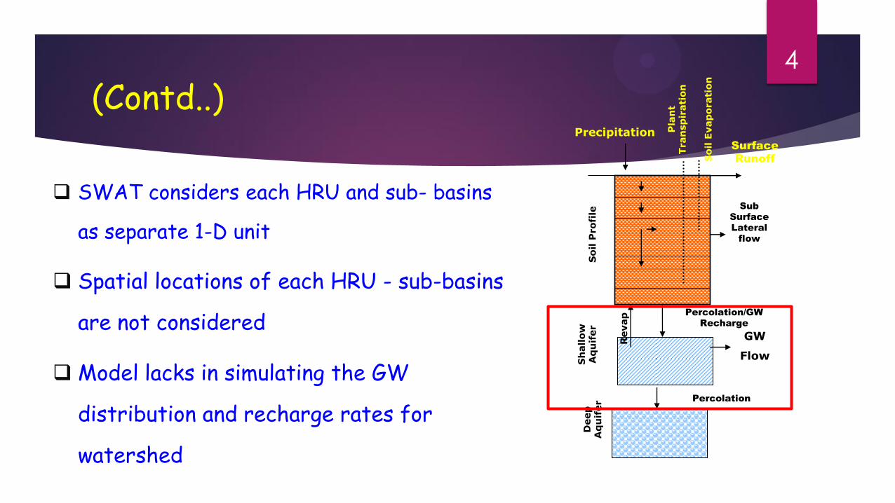
(Contd..) 4
Surface
Runoff
Sub
Surface
Lateral
flow
GW
Flow
Percolation/GW
Recharge
Pla
nt
Tran
sp
irati
on
So
il E
vap
orati
on
Precipitation
Percolation
Revap
Sh
allo
w
Aq
uif
er
Deep
A
qu
ifer
So
il P
ro
file
SWAT considers each HRU and sub- basins
as separate 1-D unit
Spatial locations of each HRU - sub-basins
are not considered
Model lacks in simulating the GW
distribution and recharge rates for
watershed
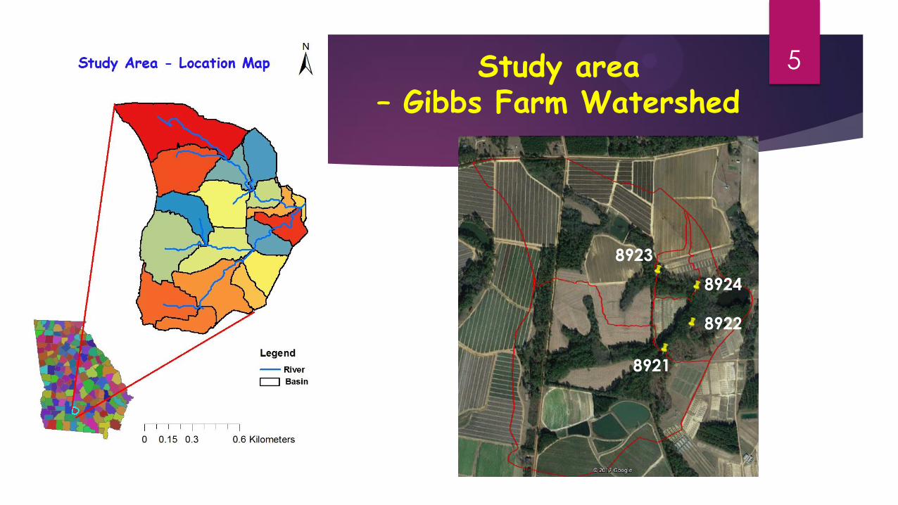
Study area – Gibbs Farm Watershed
5
8923
8924
8922
8921
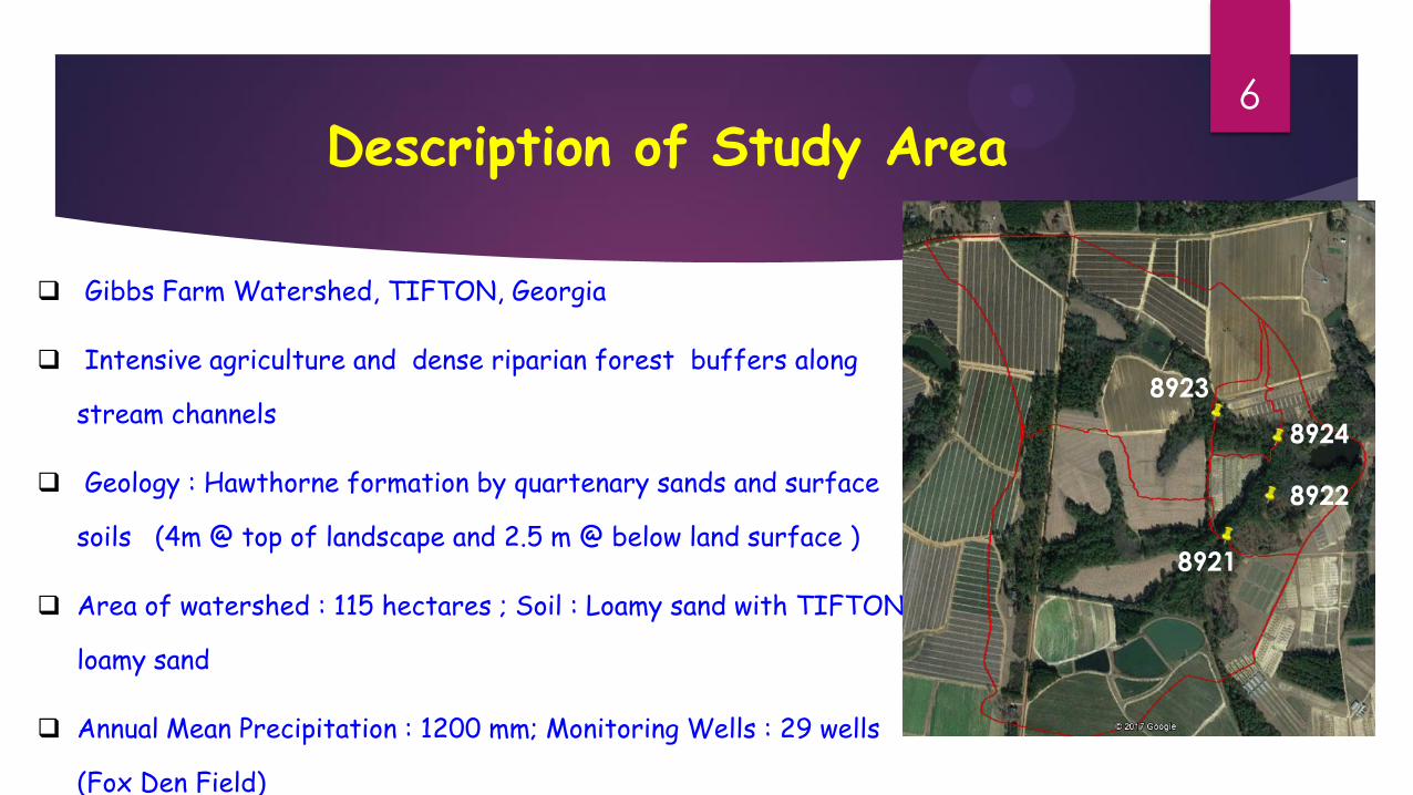
Description of Study Area
Gibbs Farm Watershed, TIFTON, Georgia
Intensive agriculture and dense riparian forest buffers along
stream channels
Geology : Hawthorne formation by quartenary sands and surface
soils (4m @ top of landscape and 2.5 m @ below land surface )
Area of watershed : 115 hectares ; Soil : Loamy sand with TIFTON
loamy sand
Annual Mean Precipitation : 1200 mm; Monitoring Wells : 29 wells
(Fox Den Field)
6
8923
8924
8922
8921
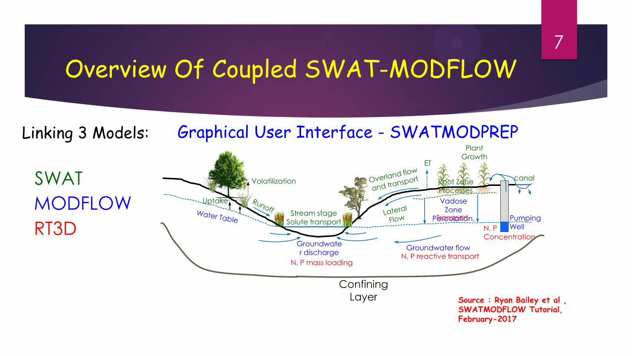
Linking 3 Models:
SWAT
MODFLOW
RT3D
Volatilization canal
Pumping Well
Vadose Zone
Percolation,
N, P
Concentration
Stream stage Solute transport
Root Zone Processes
Groundwate
r discharge Groundwater flow
Uptake
ET
Confining
Layer
Plant Growth
N, P mass loading N, P reactive transport
Transport
Overview Of Coupled SWAT-MODFLOW
7
Source : Ryan Bailey et al , SWATMODFLOW Tutorial, February-2017
Graphical User Interface - SWATMODPREP
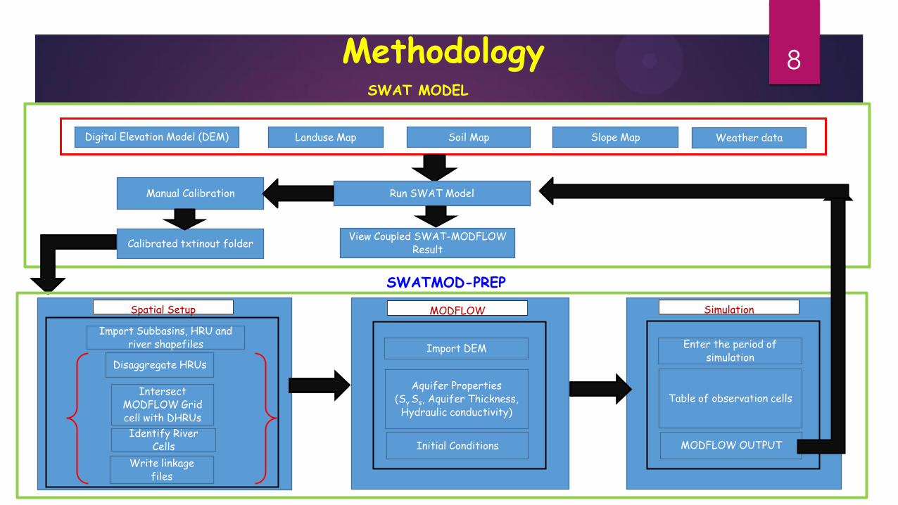
Methodology 8
Digital Elevation Model (DEM) Landuse Map Soil Map Slope Map Weather data
Run SWAT Model
Calibrated txtinout folder
SWAT MODEL
Aquifer Properties (Sy
Ss, Aquifer Thickness, Hydraulic conductivity)
Import DEM
Initial Conditions
MODFLOW
Intersect MODFLOW Grid cell with DHRUs
Identify River Cells
Write linkage files
Disaggregate HRUs
Import Subbasins, HRU and river shapefiles
Spatial Setup
Table of observation cells
Enter the period of simulation
MODFLOW OUTPUT
Simulation
SWATMOD-PREP
Manual Calibration
View Coupled SWAT-MODFLOW Result
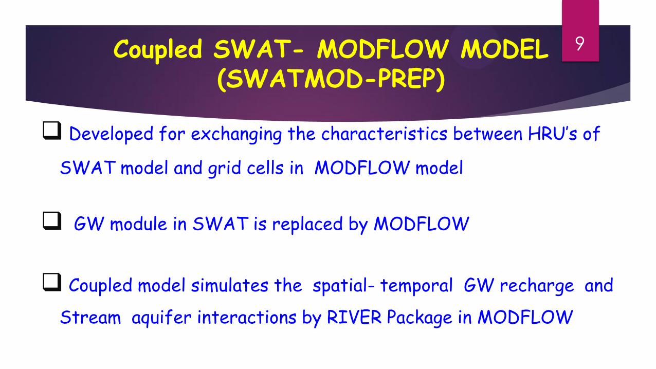
Coupled SWAT- MODFLOW MODEL (SWATMOD-PREP)
Developed for exchanging the characteristics between HRU’s of
SWAT model and grid cells in MODFLOW model
GW module in SWAT is replaced by MODFLOW
Coupled model simulates the spatial- temporal GW recharge and
Stream aquifer interactions by RIVER Package in MODFLOW
9
10
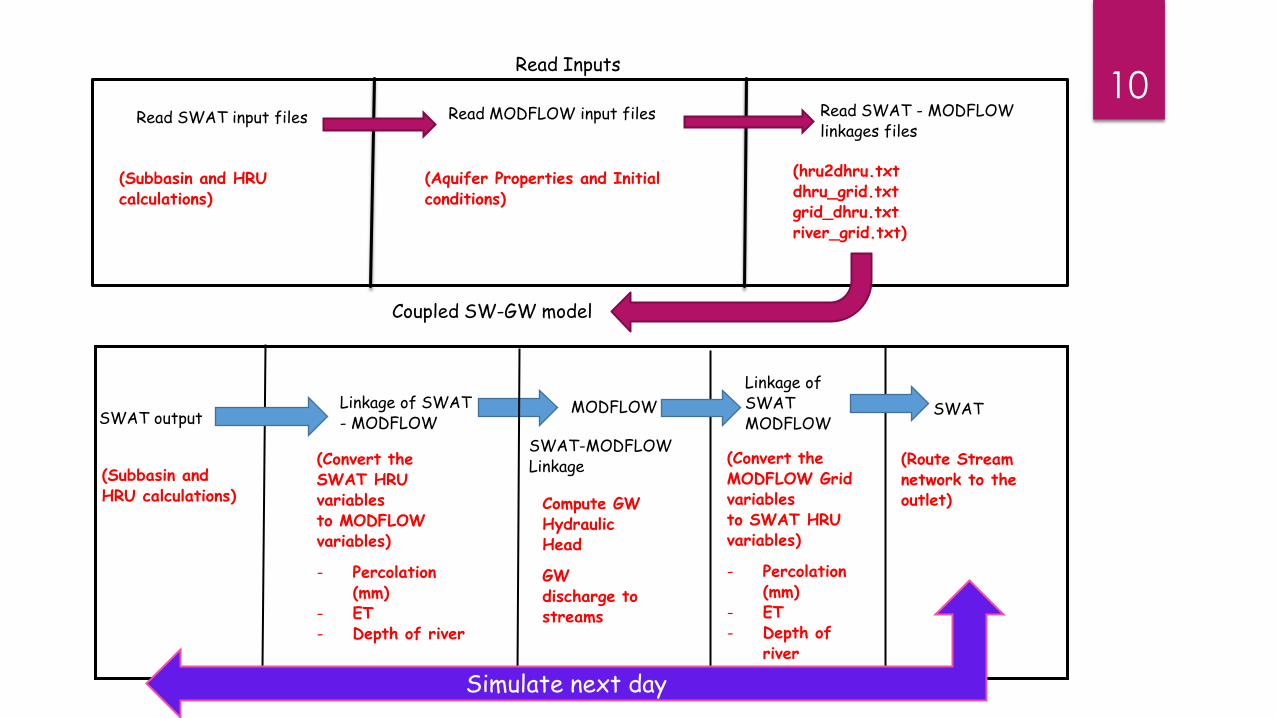
SWAT-MODFLOW Linkage
Linkage of SWAT MODFLOW
(Convert the MODFLOW Grid variables to SWAT HRU variables)
- Percolation (mm)
- ET
- Depth of river
Read SWAT - MODFLOW linkages files
Read Inputs
Read SWAT input files Read MODFLOW input files
(hru2dhru.txt dhru_grid.txt grid_dhru.txt river_grid.txt)
(Aquifer Properties and Initial conditions)
(Subbasin and HRU calculations)
(Convert the SWAT HRU variables to MODFLOW variables)
- Percolation (mm)
- ET
- Depth of river
(Subbasin and HRU calculations)
MODFLOW SWAT output
Coupled SW-GW model
Linkage of SWAT - MODFLOW
SWAT
(Route Stream network to the outlet)
Compute GW Hydraulic Head
GW discharge to streams
Simulate next day

SWAT Model Input Data
11

SWAT Model Input Data
12
Landuse : North basin (more crops in plastic covered beds) and south basin ( more ponds and less land for crops)
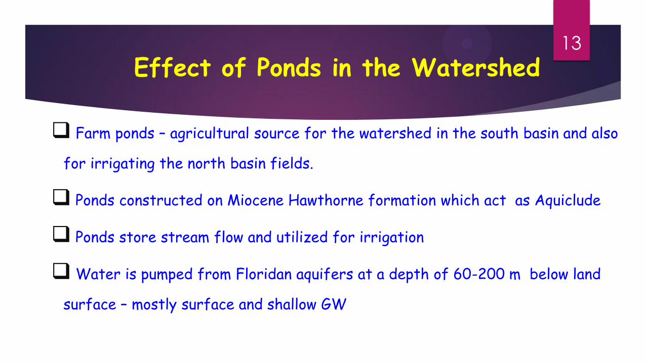
Effect of Ponds in the Watershed
13
Farm ponds – agricultural source for the watershed in the south basin and also
for irrigating the north basin fields.
Ponds constructed on Miocene Hawthorne formation which act as Aquiclude
Ponds store stream flow and utilized for irrigation
Water is pumped from Floridan aquifers at a depth of 60-200 m below land
surface – mostly surface and shallow GW
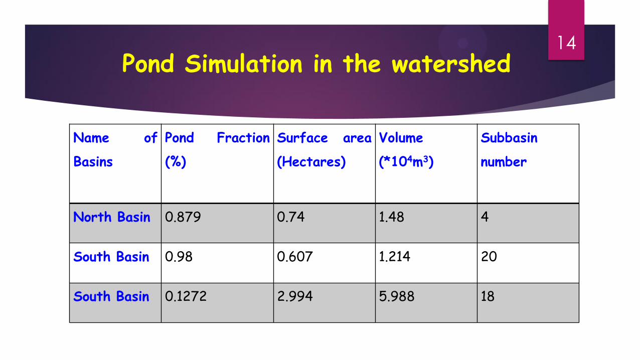
Pond Simulation in the watershed
14
Name of
Basins
Pond Fraction
(%)
Surface area
(Hectares)
Volume
(*104m3)
Subbasin
number
North Basin 0.879 0.74 1.48 4
South Basin 0.98 0.607 1.214 20
South Basin 0.1272 2.994 5.988 18

SWAT Model Setup
Simulation periods : January 1995 through December 2004
Warm up period : January 1995 through December 1997
Calibration sites : U/S Stream gauge :8924 ; D/s Stream gauge : 8922
Validation sites : U/S stream gauge : 8923 ; D/s Stream gauge : 8921
Observed data : Stream flow ( January 1998-December 2004)
Model performance indices : NSE and R2
Pond simulation in both north and south basin
15
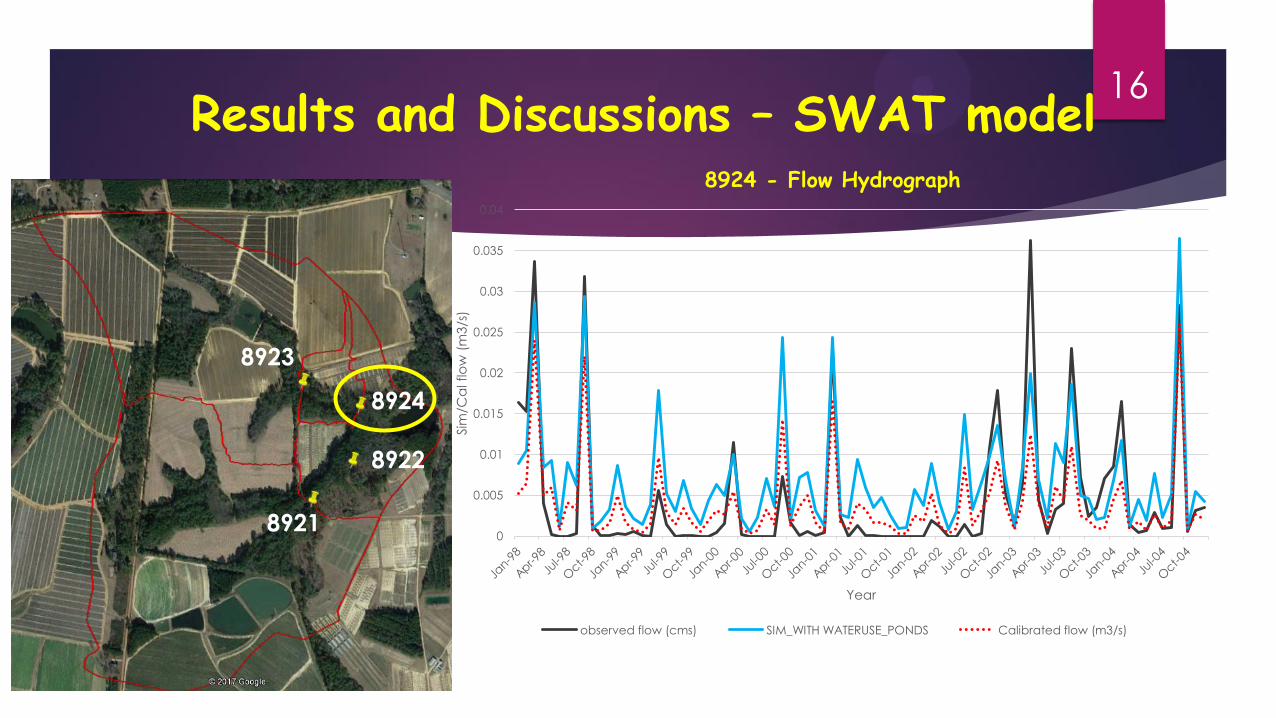
Results and Discussions – SWAT model
16
0
0.005
0.01
0.015
0.02
0.025
0.03
0.035
0.04
Sim
/Ca
l flo
w (
m3/s
)
Year
8924 - Flow Hydrograph
observed flow (cms) SIM_WITH WATERUSE_PONDS Calibrated flow (m3/s)
8923
8924
8922
8921
(Contd..)
17
0
0.005
0.01
0.015
0.02
0.025
0.03
0.035
0.04
0.045
0.05
Ja
n-9
8
Ma
r-9
8
Ma
y-9
8
Ju
l-9
8
Se
p-9
8
No
v-9
8
Ja
n-9
9
Ma
r-9
9
Ma
y-9
9
Ju
l-9
9
Se
p-9
9
No
v-9
9
Ja
n-0
0
Ma
r-0
0
Ma
y-0
0
Ju
l-0
0
Se
p-0
0
No
v-0
0
Ja
n-0
1
Ma
r-0
1
Ma
y-0
1
Ju
l-0
1
Se
p-0
1
No
v-0
1
Ja
n-0
2
Ma
r-0
2
Ma
y-0
2
Ju
l-0
2
Se
p-0
2
No
v-0
2
Ja
n-0
3
Ma
r-0
3
Ma
y-0
3
Ju
l-0
3
Se
p-0
3
No
v-0
3
Ja
n-0
4
Ma
r-0
4
Ma
y-0
4
Ju
l-0
4
Se
p-0
4
No
v-0
4
Sim
/Ca
l flo
w (
m3/s
)
Year
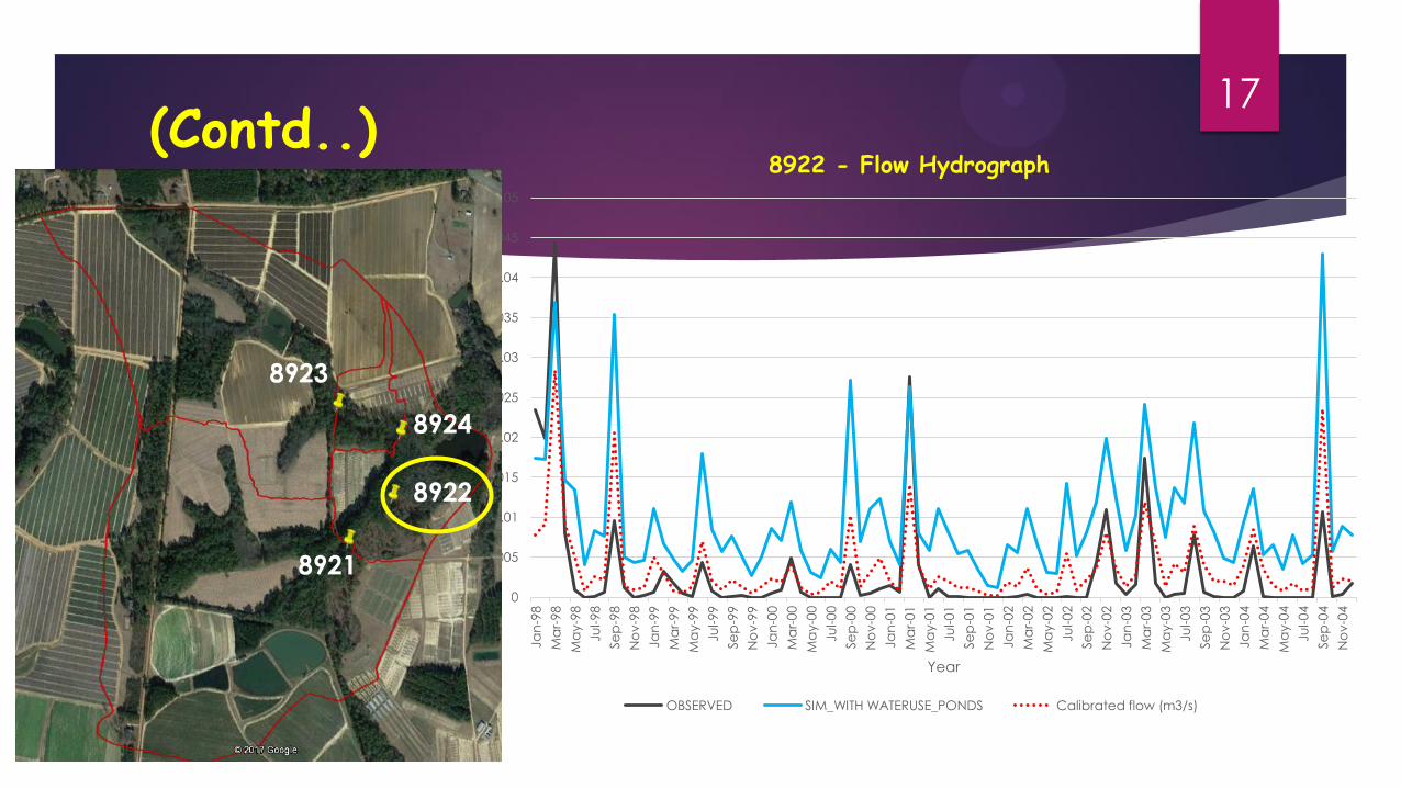
8922 - Flow Hydrograph
OBSERVED SIM_WITH WATERUSE_PONDS Calibrated flow (m3/s)
8923
8924
8922
8921
18
0
0.005
0.01
0.015
0.02
0.025
0.03
0.035
Ja
n-9
8
Ma
r-9
8
Ma
y-9
8
Ju
l-9
8
Se
p-9
8
No
v-9
8
Ja
n-9
9
Ma
r-9
9
Ma
y-9
9
Ju
l-9
9
Se
p-9
9
No
v-9
9
Ja
n-0
0
Ma
r-0
0
Ma
y-0
0
Ju
l-0
0
Se
p-0
0
No
v-0
0
Ja
n-0
1
Ma
r-0
1
Ma
y-0
1
Ju
l-0
1
Se
p-0
1
No
v-0
1
Ja
n-0
2
Ma
r-0
2
Ma
y-0
2
Ju
l-0
2
Se
p-0
2
No
v-0
2
Ja
n-0
3
Ma
r-0
3
Ma
y-0
3
Ju
l-0
3
Se
p-0
3
No
v-0
3
Ja
n-0
4
Ma
r-0
4
Ma
y-0
4
Ju
l-0
4
Se
p-0
4
No
v-0
4
Sim
/Ca
l flo
w (
m3/s
)
Year
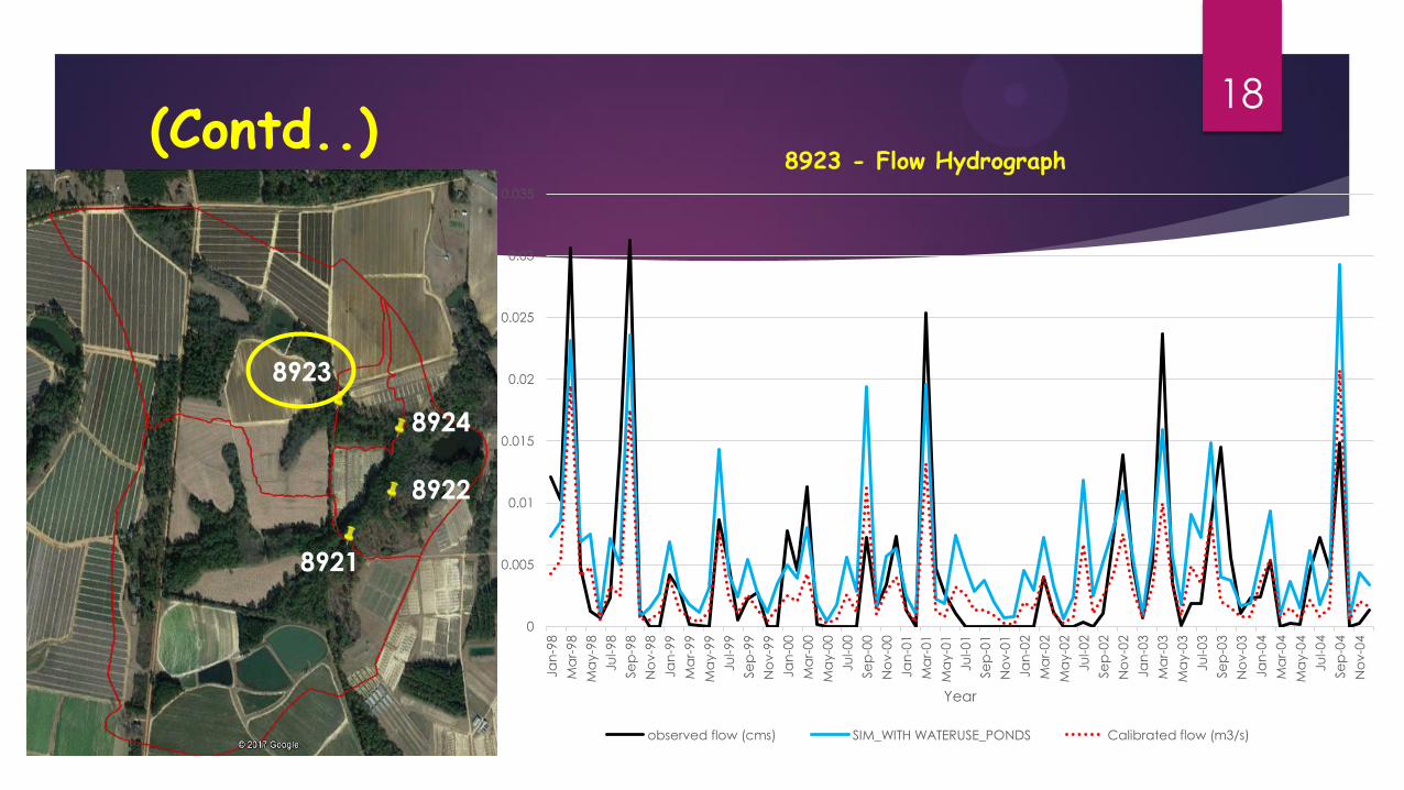
8923 - Flow Hydrograph
observed flow (cms) SIM_WITH WATERUSE_PONDS Calibrated flow (m3/s)
8923
8924
8922
8921
(Contd..)

19
0
0.005
0.01
0.015
0.02
0.025
0.03
0.035
0.04
0.045
Ja
n-9
8
Ma
r-9
8
Ma
y-9
8
Ju
l-9
8
Se
p-9
8
No
v-9
8
Ja
n-9
9
Ma
r-9
9
Ma
y-9
9
Ju
l-9
9
Se
p-9
9
No
v-9
9
Ja
n-0
0
Ma
r-0
0
Ma
y-0
0
Ju
l-0
0
Se
p-0
0
No
v-0
0
Ja
n-0
1
Ma
r-0
1
Ma
y-0
1
Ju
l-0
1
Se
p-0
1
No
v-0
1
Ja
n-0
2
Ma
r-0
2
Ma
y-0
2
Ju
l-0
2
Se
p-0
2
No
v-0
2
Ja
n-0
3
Ma
r-0
3
Ma
y-0
3
Ju
l-0
3
Se
p-0
3
No
v-0
3
Ja
n-0
4
Ma
r-0
4
Ma
y-0
4
Ju
l-0
4
Se
p-0
4
No
v-0
4
Sim
/Ca
l flo
w (
m3/s
)
Year
8921 - Flow Hydrograph
OBSERVED SIM_WITH WATERUSE_PONDS Calibrated flow (m3/s)
8923
8924
8922
8921
(Contd..)
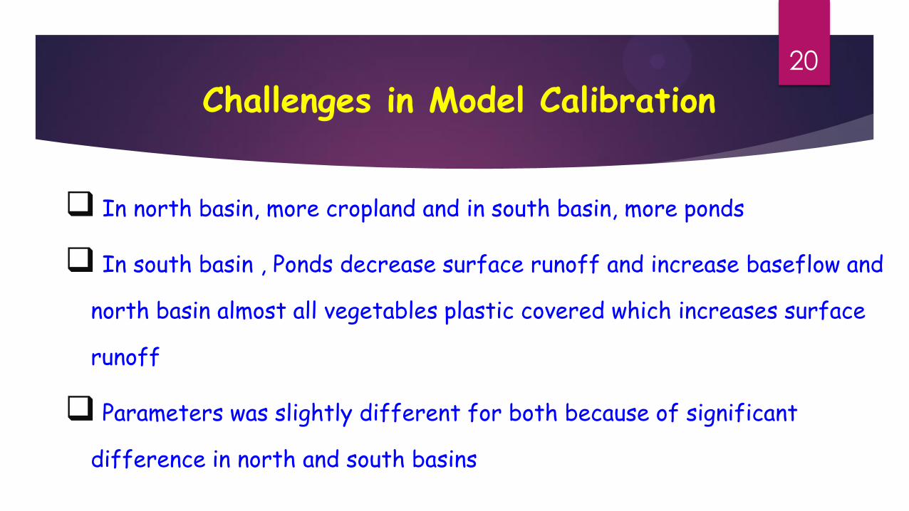
Challenges in Model Calibration
In north basin, more cropland and in south basin, more ponds
In south basin , Ponds decrease surface runoff and increase baseflow and
north basin almost all vegetables plastic covered which increases surface
runoff
Parameters was slightly different for both because of significant
difference in north and south basins
20
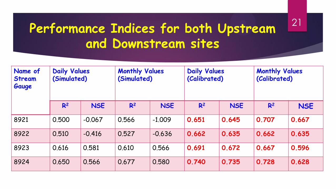
Performance Indices for both Upstream and Downstream sites
21
Name of Stream Gauge
Daily Values (Simulated)
Monthly Values (Simulated)
Daily Values (Calibrated)
Monthly Values (Calibrated)
R2 NSE R2 NSE R2 NSE R2 NSE
8921 0.500 -0.067 0.566 -1.009 0.651 0.645 0.707 0.667
8922 0.510 -0.416 0.527 -0.636 0.662 0.635 0.662 0.635
8923 0.616 0.581 0.610 0.566 0.691 0.672 0.667 0.596
8924 0.650 0.566 0.677 0.580 0.740 0.735 0.728 0.628
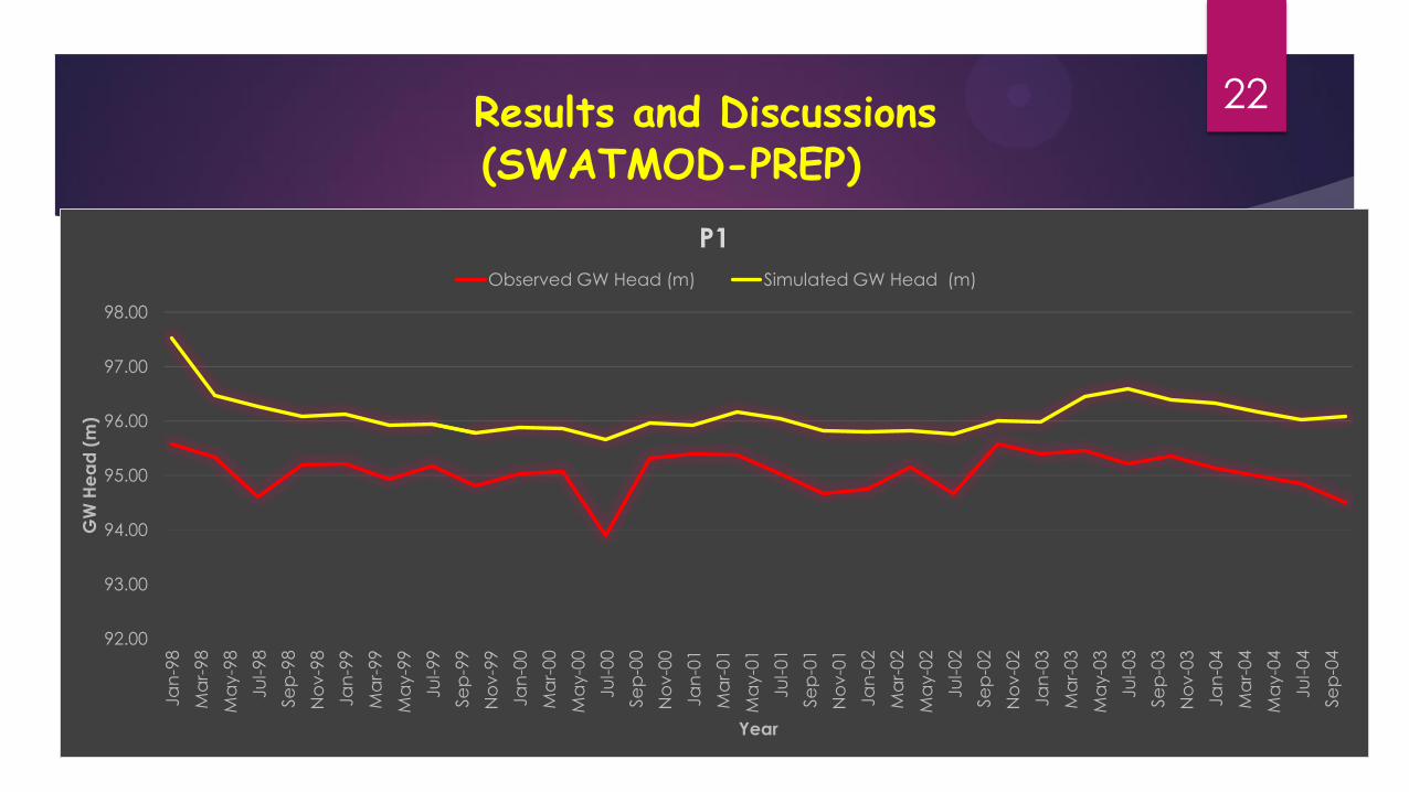
Results and Discussions (SWATMOD-PREP)
22
92.00
93.00
94.00
95.00
96.00
97.00
98.00
Ja
n-9
8
Ma
r-98
Ma
y-9
8
Ju
l-98
Se
p-9
8
No
v-9
8
Ja
n-9
9
Ma
r-99
Ma
y-9
9
Ju
l-99
Se
p-9
9
No
v-9
9
Ja
n-0
0
Ma
r-00
Ma
y-0
0
Ju
l-00
Se
p-0
0
No
v-0
0
Ja
n-0
1
Ma
r-01
Ma
y-0
1
Ju
l-01
Se
p-0
1
No
v-0
1
Ja
n-0
2
Ma
r-02
Ma
y-0
2
Ju
l-02
Se
p-0
2
No
v-0
2
Ja
n-0
3
Ma
r-03
Ma
y-0
3
Ju
l-03
Se
p-0
3
No
v-0
3
Ja
n-0
4
Ma
r-04
Ma
y-0
4
Ju
l-04
Se
p-0
4
GW
He
ad
(m
)
Year
P1
Observed GW Head (m) Simulated GW Head (m)

(CONTD..)
23
90.00
92.00
94.00
96.00
98.00
100.00
102.00
104.00
GW
HEA
D (
M)
YEAR
P3
Observed GW Head (m) Simulated GW Head (m)

(CONTD..)
24
91.5
92
92.5
93
93.5
94
94.5
95
95.5
96
96.5
GW
HEA
D (
M)
YEAR
8906
Observed_8906 Simulated_8906
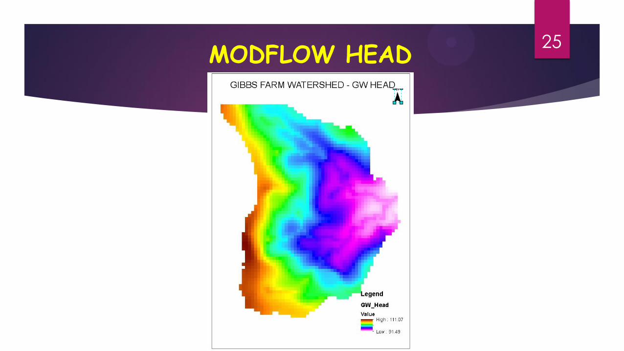
MODFLOW HEAD
25
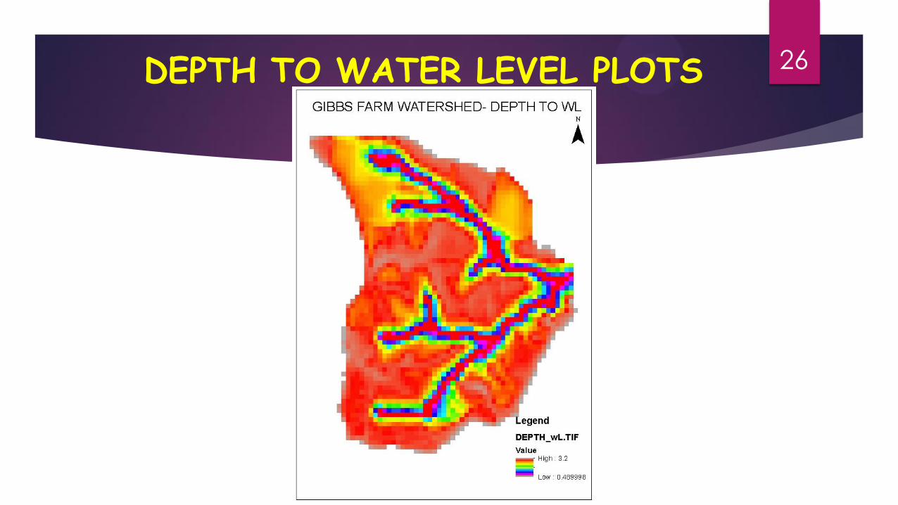
DEPTH TO WATER LEVEL PLOTS 26

SWAT RECHARGE 27
Recharge values range from 0 –3.19 m

GW SW INTERACTION SWAT
28
Seepage to aquifer range from -1.48 to -167.91 m3/d
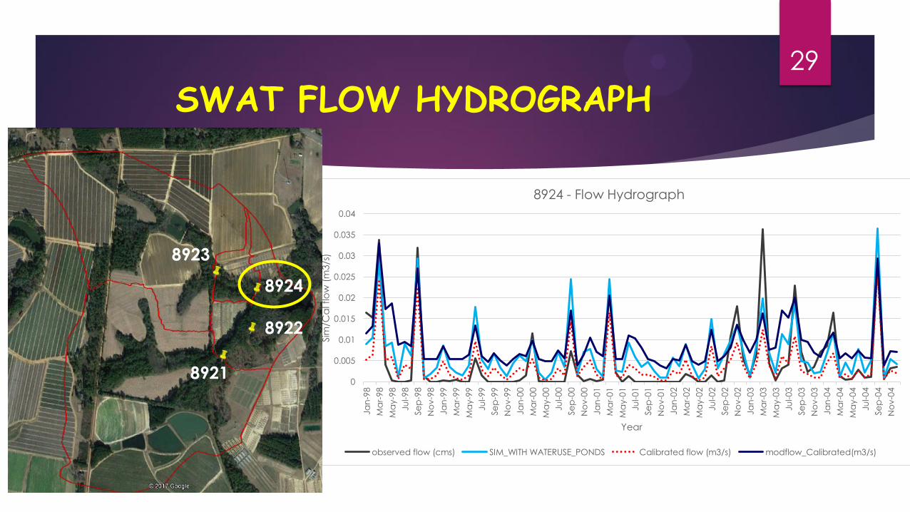
SWAT FLOW HYDROGRAPH
29
0
0.005
0.01
0.015
0.02
0.025
0.03
0.035
0.04
Ja
n-9
8
Ma
r-9
8
Ma
y-9
8
Ju
l-9
8
Se
p-9
8
No
v-9
8
Ja
n-9
9
Ma
r-9
9
Ma
y-9
9
Ju
l-9
9
Se
p-9
9
No
v-9
9
Ja
n-0
0
Ma
r-0
0
Ma
y-0
0
Ju
l-0
0
Se
p-0
0
No
v-0
0
Ja
n-0
1
Ma
r-0
1
Ma
y-0
1
Ju
l-0
1
Se
p-0
1
No
v-0
1
Ja
n-0
2
Ma
r-0
2
Ma
y-0
2
Ju
l-0
2
Se
p-0
2
No
v-0
2
Ja
n-0
3
Ma
r-0
3
Ma
y-0
3
Ju
l-0
3
Se
p-0
3
No
v-0
3
Ja
n-0
4
Ma
r-0
4
Ma
y-0
4
Ju
l-0
4
Se
p-0
4
No
v-0
4
Sim
/Ca
l flo
w (
m3/s
)
Year
8924 - Flow Hydrograph
observed flow (cms) SIM_WITH WATERUSE_PONDS Calibrated flow (m3/s) modflow_Calibrated(m3/s)
8923
8924
8922
8921
Findings and Future work
SWAT model need to calibrated for SW processes
MODFLOW model need to be calibrated for GW processes
Comparative study of SWAT model with numerical techniques (Finite
Element Method and Finite Difference Method) and Analytic
Techniques (Analytic Element Method)
30

Thank You For Your Attention
31