Embed Size (px)
Citation preview

COMPARATIVE EVALUATION OF SIX DIFFERENT GRANULAR ACTIVATED CARBON FOR TCP REMOVAL USING
RAPID SMALL SCALE COLUMN TEST
A THESIS SUBMITTED TO THE GRADUATE DIVISION OF THE UNIVERSITY OF HAWAI‘I AT MĀNOA IN PARTIAL FULFILLMENT
OF THE REQUIREMENTS FOR THE DEGREE OF
MASTER OF SCIENCE
IN
CIVIL ENGINEERING
DECEMBER 2014
By
Bryce K. Harada
Thesis Committee:
Roger W. Babcock Jr, Chairperson Sayed M. Bateni Michelle H. Teng
Keywords: Granular Activated Carbon, Trichloropropane, Breakthrough

i
COPYRIGHT © 2014 BRYCE K. HARADA
ALL RIGHTS RESERVED

ii
DEDICATED
To
My Mother, Rae Harada: Thank you for your unconditional love and support,
for pushing me through school, and for all that you have sacrificed for me.
None of this would be possible without you.
My Father, Perry Harada: Thank you for your unconditional love and support,
for teaching me to always be humble and to always show respect,
and for sharing your humor and passion for music with me. Proud to be a Harada.
My Aunty, Roanne Tsutsui:
Thank you for all you have done for me in my life, for your help throughout my education, for sharing your knowledge about life,
and most importantly, for accepting me like a son. You are the best aunty ever.
Uncle Jay:
Thank you for all your love and for being my #1 fan. You are everything I could ask in an uncle
Uncle Kenny:
Can’t even begin to say how thankful I am to have you as an uncle. I hope I made you proud, as a runner and as a person.
Uncle Roy:
Thank you for all your kindness. I appreciate your always letting me stay over and helping me out.
Grandma:
Thank you for being the best grandma ever. The goodies and ice cream money always hit the spot,
but it meant more to me just to visit you. Love, Bryce-Man.

iii
Grandpa:
Thank you for being the best grandpa in the universe. I would give up everything just to see you again.
I loved going to KTA with you, and enjoyed hearing the same stories. You could always bring a smile to my face. I know one day we will be together again.
My sister, Brandy Harada:
Thank you for being a great sister, and for giving me all your love and support;
it was unconditional for the most part, I think. And thanks for the awesome inside jokes.
My girlfriend, Maya Yamane:
Thank you for always being by my side and for putting up with me and my stressed-out self.
You could always brighten the darkest of days.
I’m blessed to have so many great people in my life. Words cannot express how much you all mean to me.
I love each and every one of you!

iv
ACKNOWLEDGEMENTS
I would like to thank everyone who has helped and supported me throughout my
research project.
First, I would like to thank Dr. Roger Babcock, Jr., for giving me the opportunity
to do this research project. You were always encouraging, made work a joy, and never
got mad at me. I am truly glad I was lucky enough to have you as an advisor.
Second, I would like to thank all the other Ph.D. and Master’s Degree students at
the Environmental Lab. Yanling Li, thank you for all your support and for your many late
night samplings. I could always count on you. You are very knowledgeable, but kept
things light with your humor. Leonardo Postacchini, thank you also for your late night
samplings and for helping me with extractions. It was always a pleasure working with
you. Gloria Cheong, thank you for all your help and for being a good friend to me.
Krishna L, thank you for going out of your way to teach and help me, even though you
weren’t on the project. Colin Nguyen, thank you for your many early morning samplings
and for never complaining. I appreciate the hard work and friendship from each and
every one of you. I will miss all of you very much.
Third, I would like to thank the AECOM workers, Lambert Yamashita, Fan Feng,
and Suengdon Joo, who were all a joy to work with. I would also like to thank GAC
expert, Adam Redding, for sharing his knowledge of RSSCT.
Fourth, I would like to thank Amy Fujishige for encouraging me to become a
research assistant and making the graduation process easy for me. You were always on
top of it, and whenever I had a problem, you were able to solve it.
Finally, I would like to say thank you to everyone who helped me throughout this
journey and apologize if I left anyone out!

v
ABSTRACT
A Constant Diffusivity-Rapid Small-Scale Column Test (CD-RSSCT) was performed
to estimate the Granular Activated Carbon (GAC) usage rates of six different activated
carbons for 1,2,3-Trichloropropane (TCP) removal. TCP is a synthetic chemical
compound contained in industrial solvents and soil fumigants and is believed to be a
human carcinogen. The State of Hawaii’s current maximum contaminant level (MCL) for
TCP is 600 parts per trillion (ppt), but consideration is being given to lower this MCL to 5
ppt. GAC adsorption is an efficient water treatment technique used to remove natural
and synthetic organic compounds, chlorine, and some metals. The GAC is housed in
contact columns at water treatment facilities. For this research, three separate Board
of Water Supply (BWS) water treatment facilities on Oahu were selected as water
sources for GAC adsorption tests. This project was conducted in collaboration with
AECOM, a multinational consulting engineering firm with a branch office in Honolulu,
Hawaii.
The objectives of this study were to determine whether any GAC could meet the
possible new 5 ppt MCL for TCP, and if so, which type of GAC would be the most
effective for TCP removal. In addition, as a preliminary step, it was necessary to create a
method to quantify TCP at the 1 ppt level in order to conduct the study. This was
accomplished by modifying an EPA method; this is the first such achievement in Hawaii.
The GAC type that is able to treat the most bed-volumes at the selected breakthrough
points was determined and recommended to replace the currently GAC used in Hawaii’s
water treatment facilities.
From the RSSCT results, numerous key findings were made. (1) Any of the 6
GACs tested can meet the new possible MCL of 5 ppt for TCP, (2) GAC C, the currently
GAC used, was by far the least effective GAC in each of the three water well sites, (3)
there was no one GAC that was the most effective for all three well sites; therefore, it is
necessary to find a most effective GAC type specific to the well site, (4) the most
effective GAC for Kunia I was GAC A/B and D, for Waipahu III was GAC E, and for Mililani
I was GAC A/B, (5) the smaller the GAC particle size, the less effective the GAC was, (6)

vi
the water matrix affected TCP adsorption, and (7) along with TCP, EDB and DBCP
removal will also be taken into consideration for the GAC selection. The findings from
this RSSCT study are of great value and significance. The fact that current GAC was the
least effective is very insightful because it means that the selection of any of the other
GACs would improve the GAC process performance in the field. Replacing the current
GAC unit with a more effective one means the GAC units would need to be changed less
frequently, thus saving on maintenance and operating costs.

vii
Table of Contents DEDICATED ....................................................................................................................................... ii
ACKNOWLEDGEMENTS ................................................................................................................... iv
ABSTRACT ......................................................................................................................................... v
1 INTRODUCTION ........................................................................................................................ 1
1.1 Project Background .......................................................................................................... 1
1.2 Problem Statement .......................................................................................................... 2
1.3 Objective .......................................................................................................................... 2
1.4 Selected GACs and Water Well Sites ............................................................................... 3
2 BACKGROUND .......................................................................................................................... 5
2.1 1, 2, 3-Trichloropropane (TCP) ......................................................................................... 5
2.1.1 What is TCP? ............................................................................................................ 5
2.1.2 TCP Importance ........................................................................................................ 6
2.1.3 TCP Health Side Effects ............................................................................................ 6
2.1.4 TCP in the Environment and Groundwater Contamination ..................................... 7
2.1.5 TCP Exposure ............................................................................................................ 8
2.1.6 TCP Introduction to Hawaii ...................................................................................... 8
2.1.7 California and Hawaii’s TCP Regulations ................................................................ 11
2.1.8 Existing Federal and State Guidelines and Health Standards for TCP ................... 11
2.1.9 TCP Detection Methods ......................................................................................... 12
2.1.10 TCP Treatment (Sources) ....................................................................................... 12
2.1.11 TCP Production and Disposal ................................................................................. 13
2.2 Granular Activated Carbon (GAC) .................................................................................. 14
2.2.1 What is GAC?.......................................................................................................... 14
2.2.2 Description of Processes ........................................................................................ 16
2.2.3 GAC Particle Sizes ................................................................................................... 19
2.2.4 GAC Treatment Units ............................................................................................. 19
2.2.5 Key Concepts .......................................................................................................... 21
2.2.6 GAC column configuration ..................................................................................... 22
2.2.7 Handling of Spent/Exhausted GAC......................................................................... 22
2.2.8 Adsorption Isotherms ............................................................................................ 23

viii
2.3 Rapid Small Scale Column Test ...................................................................................... 25
2.3.1 Approach ................................................................................................................ 25
2.3.2 Development of Scaling Equations ........................................................................ 26
2.3.3 Drawbacks .............................................................................................................. 30
3 METHODS AND PROCEDURES ................................................................................................ 30
3.1 Water Sample Transport and Preparation ..................................................................... 30
3.2 Analytical Details ............................................................................................................ 30
3.3 Determination of RSSCT Flow Rate ................................................................................ 31
3.4 GAC Properties ............................................................................................................... 33
3.4.1 RSSCT Test Apparatus ............................................................................................ 33
3.4.2 Reagents ................................................................................................................. 46
3.4.3 Experimental Procedures ....................................................................................... 46
3.4.4 GAC Grinding and Screening Procedure ................................................................ 46
3.5 EDB, DBCP, and TCP in Water by Microextraction and Gas Chromatography – EPA Method 504.1 ............................................................................................................................ 50
3.5.1 Approach ................................................................................................................ 50
3.5.2 Assumptions ........................................................................................................... 50
3.5.3 Procedure ............................................................................................................... 50
Data Analysis and Calculations .............................................................................................. 52
4 RESULTS AND ANALYSIS ......................................................................................................... 53
4.1 General ........................................................................................................................... 53
4.1.1 Results .................................................................................................................... 53
4.1.2 Analysis .................................................................................................................. 54
4.2 Results/Analysis by GAC Type ........................................................................................ 56
4.2.1 GAC A/B Results ..................................................................................................... 56
4.2.2 GAC A/B Analysis .................................................................................................... 57
4.2.3 GAC C Results ......................................................................................................... 58
4.2.4 GAC C Analysis ........................................................................................................ 59
4.2.5 GAC D Results ......................................................................................................... 60
4.2.6 GAC D Analysis ....................................................................................................... 61
4.2.7 GAC E Results ......................................................................................................... 62
4.2.8 GAC E Analysis ........................................................................................................ 63

ix
4.2.9 GAC F Results ......................................................................................................... 64
4.2.10 GAC F Analysis ........................................................................................................ 65
4.2.11 GAC G Results ......................................................................................................... 66
4.2.12 GAC G Analysis ....................................................................................................... 67
4.3 Comparative Analysis – GAC Effectiveness based on Average Bed-Volumes Treated .. 67
4.4 Results/Analysis by Water Well Source ......................................................................... 70
4.4.1 Kunia I Results ........................................................................................................ 70
4.4.2 Kunia I Analysis....................................................................................................... 72
4.4.3 Waipahu III v3 Results ............................................................................................ 73
4.4.4 Waipahu III v3 Analysis .......................................................................................... 75
4.4.5 Waipahu III v5 Results ............................................................................................ 76
4.4.6 Waipahu III v5 Analysis .......................................................................................... 77
4.4.7 Mililani I Results ..................................................................................................... 78
4.4.8 Mililani I Analysis .................................................................................................... 79
4.5 Comparative Analysis – GAC Effectiveness by Water Well Site ..................................... 80
4.6 Results/Analysis by GAC Particle Size ............................................................................ 81
4.6.1 GAC Particle Size Results ........................................................................................ 81
4.6.2 Different GAC Particle Size Analysis ....................................................................... 82
4.7 Error ............................................................................................................................... 84
5 CONCLUSIONS ........................................................................................................................ 85
6 REFERENCES ........................................................................................................................... 86
7 APPENDIX ............................................................................................................................... 92
7.1 Column Sizing Calculations ............................................................................................ 92
7.1.1 Full-Scale Column Parameters (Given)................................................................... 92
7.1.2 Full – Scale GAC Particle Sizes ................................................................................ 93
7.1.3 Full – Scale Reynold’s Number Parameters ........................................................... 94
7.1.4 Given Small-Scale (RSSCT) Column Parameters ..................................................... 94
7.1.5 Small-Scale (RSSCT) GAC Particle Sizes .................................................................. 95
7.1.6 Calculation for Small – Scale Parameters............................................................... 95
7.2 Raw Data ...................................................................................................................... 103
7.2.1 GAC Run #2 .......................................................................................................... 103
7.2.2 GAC Run #3 .......................................................................................................... 107
x
7.2.3 GAC Run #4 .......................................................................................................... 114
7.2.4 GAC Run #5 .......................................................................................................... 122
7.2.5 GAC Run #6 .......................................................................................................... 129
7.2.6 GAC Run #7 .......................................................................................................... 135
7.2.7 GAC Run #8 .......................................................................................................... 140
7.2.8 GAC Run #9 .......................................................................................................... 146
7.2.9 GAC Run #10 ........................................................................................................ 152
7.2.10 GAC Run #11 ........................................................................................................ 159

xi
TABLE OF TABLES
Table 1: Six Carbon Types Used ....................................................................................................... 3 Table 2: Independent Dimensionless Parameters for RSSCT Scaling Process ............................... 27 Table 3: Full and Small Scale GAC Properties (v5) ......................................................................... 33 Table 4: Color Interpretation for Result Tables ............................................................................. 54 Table 5: Influent TCP Concentration with Corresponding Breakthrough Limits ........................... 54 Table 6: GAC A/B Breakthrough Results – Bed-Volumes Treated ................................................. 56 Table 7: GAC A/B Breakthrough Results – TCP Mass Adsorbed per GAC Unit .............................. 56 Table 8: GAC C Breakthrough Results – Bed-Volumes Treated ..................................................... 58 Table 9: GAC C Breakthrough Results – TCP Mass Adsorbed per GAC Unit .................................. 58 Table 10: GAC D Breakthrough Results – Bed-Volumes Treated ................................................... 60 Table 11: GAC D Breakthrough Results – TCP Mass Adsorbed per GAC Unit ................................ 60 Table 12: GAC E Breakthrough Results – Bed-Volumes Treated ................................................... 62 Table 13: GAC E Breakthrough Results – TCP Mass Adsorbed per GAC Unit ................................ 62 Table 14: GAC F Breakthrough Results – Bed-Volumes Treated ................................................... 64 Table 15: GAC F Breakthrough Results – TCP Mass Adsorbed per GAC Unit ................................ 64 Table 16: GAC G Breakthrough Results – Bed-Volumes Treated ................................................... 66 Table 17: GAC G Breakthrough Results – TCP Adsorbed per GAC Mass ........................................ 66 Table 18: Average Bed-Volumes Treated ...................................................................................... 67 Table 19: Ranking GAC Effectiveness by GAC Type – Average Bed-Volumes Treated .................. 68 Table 20: Average TCP Mass Adsorbed per GAC Unit ................................................................... 68 Table 21: Ranking Effectiveness by GAC Type – Average TCP Mass Adsorbed per GAC Unit ....... 68 Table 22: Kunia I Breakthrough Results – Bed-Volumes Treated .................................................. 70 Table 23: Kunia I – Effectiveness of GAC........................................................................................ 70 Table 24: Kunia I Breakthrough Results – TCP Mass Adsorbed per GAC Unit ............................... 70 Table 25: Waipahu III v3 Breakthrough Results – Bed-Volumes Treated ...................................... 73 Table 26: Waipahu III v3 – Effectiveness of GAC ........................................................................... 73 Table 27: Waipahu III v3 Breakthrough Results – TCP Mass Adsorbed per GAC Unit ................... 73 Table 28: Waipahu III v5 Breakthrough Results – Bed-Volumes Treated ...................................... 76 Table 29: Waipahu III v5 – Effectiveness of GAC ........................................................................... 76 Table 30: Waipahu III v5 Breakthrough Results – TCP Mass Adsorbed per GAC Unit ................... 76 Table 31: Mililani I Breakthrough Results – Bed-Volumes Treated ............................................... 78 Table 32: Mililani I – Effectiveness of GAC ..................................................................................... 78 Table 33: Mililani I Breakthrough Results – TCP Mass Adsorbed per GAC Unit ............................ 78 Table 34: GAC Effectiveness by Water Well Site ........................................................................... 80 Table 35: Most and Least Effective GAC by Water Well SIte ......................................................... 80 Table 36: Properties of GAC Particle Size ...................................................................................... 81 Table 37: GAC Particle Size Breakthrough Results – Bed-Volumes Treated .................................. 81 Table 38: GAC Particle Size – Effectiveness ................................................................................... 81 Table 39: GAC Particle Size Breakthrough Results – TCP Mass Adsorbed per GAC Unit ............... 81

xii
TABLE OF FIGURES
Figure 1: Map of GAC Water Treatment Facilities ........................................................................... 4 Figure 2: TCP Chemical Structure ..................................................................................................... 5 Figure 3: Physical and Chemical Properties of TCP .......................................................................... 6 Figure 4: Closed Water Wells on Oahu from EDB and DBCP Discovery ........................................ 10 Figure 5: NPL Sites with TCP Contamination ................................................................................. 10 Figure 6: Full-Scale Granular Activated Carbon ............................................................................. 15 Figure 7: Small-Scale Granular Activated Carbon .......................................................................... 15 Figure 8: Granular Activated Carbon Adsorption Process ............................................................. 16 Figure 9: Flow Diagram of Zones in Carbon Bed ............................................................................ 17 Figure 10: Mass Transfer in Adsorber ............................................................................................ 18 Figure 11: Post Filtration Adsorption Unit ..................................................................................... 20 Figure 12: Filtration/Adsorption Unit ............................................................................................ 20 Figure 13: Actual RSSCT Test Apparatus ........................................................................................ 35 Figure 14: Small Scale GAC Column ............................................................................................... 36 Figure 15: GAC Column During a Run ............................................................................................ 36 Figure 16: Metal Threads ............................................................................................................... 37 Figure 17: Liquid Metering Pumps ................................................................................................. 38 Figure 18: Pressure Gauge ............................................................................................................. 38 Figure 19: Water Containers .......................................................................................................... 39 Figure 20: Effluent Water Samples ................................................................................................ 40 Figure 21: Auto-sampler Vial ......................................................................................................... 41 Figure 22: Drying Oven .................................................................................................................. 41 Figure 23: Refrigerator ................................................................................................................... 42 Figure 24: Extraction Set-Up .......................................................................................................... 43 Figure 25: Effluent Containers ....................................................................................................... 44 Figure 26: Data Log Book ............................................................................................................... 45 Figure 27: GAC A/B Breakthrough Results ..................................................................................... 56 Figure 28: GAC C Breakthrough Results ......................................................................................... 58 Figure 29: GAC D Breakthrough Results ........................................................................................ 60 Figure 30: GAC E Breakthrough Results ......................................................................................... 62 Figure 31: GAC F Breakthrough Results ......................................................................................... 64 Figure 32: GAC G Breakthrough Results ........................................................................................ 66 Figure 33: Kunia I Breakthrough Results ........................................................................................ 71 Figure 34: Waipahu III v3 Breakthrough Results............................................................................ 74 Figure 35: Waipahu III v5 Breakthrough Results............................................................................ 77 Figure 36: Mililani I Breakthrough Results ..................................................................................... 79 Figure 37: GAC Particle Size Breakthrough Results ....................................................................... 82

1
1 INTRODUCTION
Project Background 1.1
A granular activated carbon (GAC) water treatment study was conducted to
evaluate six different types of granular activated carbons and determine their ability to
absorb 1,2,3-Trichloropropane (TCP), a hazardous chemical compound found in Hawaii’s
drinking water aquifers. Water samples from three separate Board of Water Supply well
source sites on Oahu were tested in this study.
Life cycle analysis of the GAC adsorber is dependent on the complex, non-steady
state, mass transfer, adsorption capacity of the specific contaminant, GAC type, and the
site-specific characteristics of the water matrix (Fotta 2012). Although GAC is an
effective technique for removal of toxic organics from drinking water or wastewater and
typically the best method for TCP removal (Veatch 2008), it is a relatively expensive
process. Full scale GAC models are usually scaled to pilot scale models; these are,
however, time consuming, expensive, and require ample supply of water. For this
reason, a quicker and more economical method was designed that could model a full-
scale GAC unit from a bench-scale test using small-scale columns. This bench-scale test,
developed by J.C. Crittenden, is called the rapid small-scale column test (RSSCT)
(Crittenden, Berrigan et al. 1986, Corwin and Summers 2010).
Based on the RSSCT results (Crittenden, Berrigan et al. 1986, Crittenden, Berrigan
et al. 1987, Crittenden, Reddy et al. 1991), this GAC system was determined to be fully
scalable. Therefore, this RSSCT method was used to compare the adsorption
performance of various GAC types and to determine the number of bed-volumes of
contaminated water that can be treated before reaching breakthrough limits in the
actual water treatment. RSSCT is explained in detail in section 2.3.
RSSCT is a low-cost, time-efficient, and simple technique. However, TCP only has
a low-moderate adsorption capacity for GAC. Hence, a larger GAC treatment system
may have to be used to be effective, which would increase treatment costs (Glenn
Dombeck and Borg , Tratnyek, Sarathy et al. 2008, Molnaa 2003).

2
The four main advantages of the RSSCT are:
1. It requires less time compared to that of pilot models.
2. It does not require extensive isotherm or kinetic studies as do some
mathematical prediction models.
3. It does not require a large quantity of water, thus making it suitable to
carry out experimentally in a laboratory.
4. It is more cost efficient compared to other models.
Problem Statement 1.2
1,2,3-Trichloropropane (TCP) was introduced to Hawaii in 1948 as an impurity
found in soil fumigants used in pineapple fields. It was in the late 1970’s that all TCP-
containing products were banned from use in Hawaii due to its potential as a human
carcinogen (Eric P. Hooker, Keri G. Fulcher et al. 2012). Although it had not been used in
Hawaii since 1977, TCP contamination persisted in Hawaii’s groundwater – a major
health concern as this groundwater was used for human consumption as drinking water.
It was necessary, therefore, that a method of TCP removal from the groundwater be
designed and implemented. Granular activated carbon (GAC) adsorption was chosen as
the treatment technique due to its efficiency. This GAC adsorption technique has been
used at water treatment facilities for some time and as technology advanced over the
years, different improved GAC prototypes were designed. Several of these prototypes,
along with the GAC model currently used by the Board of Water Supply, were tested to
determine which GAC model was the most effective for TCP removal.
Objective 1.3
The objectives of this study were to determine whether any GAC could meet the
possible new 5 ppt MCL for TCP, and if so, which type of GAC would be the most
effective for TCP removal from Hawaii’s groundwater. This was accomplished by
modifying an EPA method, a first such achievement in Hawaii. The GAC type that is able
to treat the most bed-volumes at the selected breakthrough limits would be determined

3
to be the most effective, and this GAC model would be recommended as a replacement
for the current GAC system used in Hawaii’s water treatment facilities.
Selected GACs and Water Well Sites 1.4
The following GACs were selected for analysis:
GAC ID GAC Name
A/B Calgon coconut shell carbon OLC 12x40
C Jacobi direct-activated coal based carbon 8x30 (currently
used by BWS)
D Siemens coconut shell carbon C12x30
E Siemens enhanced coconut shell carbon CX12x30
F Calgon carbon coal based carbon F400 12x40
G Jacobi coconut shell carbon 12x40
Table 1: Six Carbon Types Used
The GAC identifications and corresponding names are given in Table 1. Six
different GACs, labeled A/B through G, were selected and compared. The numbers
located after the GAC name indicate the full-scale mesh size. A GAC with “12x40”
means that the GAC particles pass through a No. 12 sieve (1.68 mm), but are retained
on a No. 40 sieve (0.425 mm). The selected GACs were from one of three
manufacturers: Calgon, Jacobi, and Siemens. The Siemens and Calgon GACs were
selected based on each company’s experience with TCP treatment, their ability to
consistently provide GAC in the quantities necessary, and a literature review.
The following three BWS well sites on Oahu were selected for the study:
1. Kunia Wells I GAC Water Treatment Facility
2. Mililani Wells I GAC Water Treatment Facility
3. Waipahu Wells III GAC Water Treatment Facility

4
Figure 1: Map of GAC Water Treatment Facilities
A map of the GAC water treatment facilities located in central Oahu, including
the three selected BWS wells, is shown in Figure 1 (AECOM 2014). The three well sites
were selected for several reasons. All three well sites have:
• Existing GAC treatment systems with room for expansion;
• Relatively elevated TCP concentrations;
• Representation of one of the three distinct cation-anion water types identified
for all the wells in the study area (excluding Waialua Wells GAC Water Treatment
Facility and Haleiwa Wells GAC Water Treatment Facility on the North Shore);
and
• Concentrations of dissolved organic carbons typical for all the wells in the study
area.

5
2 BACKGROUND
1, 2, 3-Trichloropropane (TCP) 2.1
2.1.1 What is TCP?
1,2,3-Trichloropropane (TCP) is a synthetic chlorinated hydrocarbon with a high
chemical stability (Samin and Janssen 2012). It is also known as allyl trichloride, glycerol
trichlorohydrin, and trichlorohydrin (ATSDR 1995, Administration 2013), with the
chemical formula C3H5Cl3. Its chemical structure is shown below in Figure 2 (F. Bianchi,
M. Careri et al. 2007).
Figure 2: TCP Chemical Structure
It is characterized by being colorless, heavy, and highly volatile with a sweet and
strong odor. Although its main use is to combine with other chemicals to make other
chemical compounds, it was also widely used as an industrial solvent, paint remover,
cleaning agent, and fumigant (ATSDR 1992).
TCP was an impurity contained in the Shell Chemical Company soil fumigant
product, “D-D”, which was used in Hawaii between 1948 and 1977. It was discontinued
due to its potential as a human carcinogen (see section 2.1.3). Because of TCPs inability
to decompose naturally into the environment, it is still present in Hawaii’s groundwater.
This is explained in section 2.1.4.
In 2005, the State of Hawaii established a statewide maximum contaminant level
(MCL) of 0.6 ppb (2011). It has been proposed that Hawaii significantly lower its MCL
for TCP to equal the CDPH’s notification level of 5 ppt (2010).

6
The physical and chemical properties of TCP are shown below in Figure 3
(Agency 2013).
Figure 3: Physical and Chemical Properties of TCP
2.1.2 TCP Importance
TCP is a groundwater contaminant that is a suspected human carcinogen. This
chemical compound is persistent in Oahu’s groundwater aquifers and is a cause of
concern to the general public’s health. A cost effective and feasible method for TCP
removal from contaminated water is imperative. Several options for removal are
available, but GAC is being used as the method of choice for the removal of TCP
contamination in Oahu’s groundwater.
2.1.3 TCP Health Side Effects
TCP is believed to be a human carcinogen; there are no studies, however,
proving that TCP is cancerous in humans. The only laboratory studies conducted were
performed on animals and through in vitro testing. In these animal studies, it was found
that long term effects of TCP exposure include bodyweight fluctuation, kidney problems,
and increased risk of tumors (ATSDR 1992, Agency 2013). The EPA classifies TCP as
“likely to be carcinogen to humans” ((IRIS) 2009), the U.S. Department of Health and
Human Services anticipates TCP to be a probable human carcinogen based on
carcinogenic effects on experimental animals ((DHHS) 2011), and the National Institute

7
for Occupational Safety and Health (NIOSH) classifies TCP as a potential occupational
carcinogen ((NIOSH) 2010).
Short term effects in humans exposed to TCP levels of 50 – 100 ppm over an 8-
hour time span were throat and eye irritation. It is unknown what exposure to low
levels of TCP level over a long period of time would be. The main health effect of TCP in
both animals and humans was impairment of the respiratory system (ATSDR 1995).
2.1.4 TCP in the Environment and Groundwater Contamination
In the atmosphere, TCP is predicted to only exist in the gas phase. When TCP is
exposed to sunlight, it breaks down in the air by a reaction with hydroxyl radicals. It
possesses a half-life of 15 - 46 days, thus as little as 7% of the original TCP molecules will
remain in the air after two months ((HSDB) 2009, (DHHS) 2011, Samin and Janssen
2012).
In the liquid phase, TCP is unlikely to sorb into soil because of its low soil organic
carbon-water partition coefficient. Consequently, the TCP molecules either readily
evaporate from the soil surface or leach through the soil into the groundwater (ATSDR
1992, ATSDR 1995, (HSDB) 2009). Since TCP in its pure form is a Dense Non Aqueous
Phase Liquid (DNAPL), it is both immiscible and denser than water. This allows it to
settle at the bottom of the aquifer where very minimal TCP evaporation occurs. There,
the TCP molecules accumulate over time ((Cal/EPA) 2009), and it is the reason why TCP
is still present in Oahu’s groundwater aquifers. TCP’s low abiotic and biotic degradation
rates contribute to its persistence in the groundwater. Because of this, however, TCP is
less likely to absorb into plants, fishes, and other aquatic organisms (ATSDR 1992).
There is no evidence that TCP can decompose naturally, but it may under
favorable conditions (Stepek 2009). Proper remediation techniques are vital to ensure
the safety of drinking water.

8
2.1.5 TCP Exposure
The main sources of TCP exposure in order of likeliness to occur are:
1. Inhalation via contaminated air
2. Ingestion via drinking contaminated water
3. Dermal/Ingestion via contaminated soil
4. Being in contaminated facilities
TCP exposure is most evident near a hazardous waste disposal site where TCP is
not stored properly and in areas of TCP spillage. It is not a common compound found in
the environment (air, water, soil). Low concentrations have been found in some rivers,
bays, groundwater, wells, and hazardous waste sites (ATSDR 1992).
2.1.6 TCP Introduction to Hawaii
As stated earlier, TCP was an impurity in the Shell Chemical Company soil
fumigant product, “D-D”. The amount of TCP in the D-D mixture was estimated to range
from 0.4 – 0.7% by weight; the actual values, however, might deviate from this range.
Even though TCP accounted for a only a small percentage of the total D-D content, D-D
was used at such high rates that TCP was being applied at quantities equal to or more
than most pesticides. D-D was initially manufactured in 1942, but it wasn’t until 1948
that it was introduced to Hawaii. The Dole Company and Del Monte Corporation, two
pineapple growers on Oahu, selected Shell’s D-D as its primary soil fumigant to control
nematodes in the pineapple fields (26)[26]. In the late 1970s to early 1980s, after 20 -
30 years of use in the fields, D-D use was banned due to the TCP health risks (Eric P.
Hooker, Keri G. Fulcher et al. 2012). It was reported that D-D has not been used on
Hawaii’s pineapple fields since 1977, but because of TCPs inability to decompose
naturally into the environment, it is still present in Hawaii’s groundwater.
Two companies, Shell and Dow, who manufactured these TCP containing
fumigants, purposely left TCP and other hazardous waste impurities in their products
and intentionally mislabeled their as products as “100% active” as a business tactic to
avoid the cost of having to remove and dispose of their hazardous wastes. Because of

9
this, many innocent farmers throughout the country unknowingly dumped millions of
pounds of TCP and other hazardous impurities into the ground. Valuable groundwater
was thus contaminated throughout the country and is the reason that TCP can be found
in many drinking water wells today (26)[26].
Volatile organic contamination in Hawaii was first revealed following a spilling
incident on April 7, 1977. On that day, approximately 1.9 m3 of Ethylene Dibromide
(EDB) was spilled within 18 meters of Kunia Well on Oahu. This was the first time the
State of Hawaii faced the possibility of pesticide contamination of its groundwater.
Laboratory analyses conducted a week after the incident showed EDB levels were not
detectable. The EDB detection limit of the testing apparatus was 500 ng/L (0.5 ppb), so
it was assumed that the contamination level, if any, was less than that amount. It was
suspicious, however, that such a high volume of EDB spill tested no significant
concentration levels in the groundwater. The EDB spill must have gone somewhere,
and they needed to investigate further.
In May, 1979, California wells were discovered to be contaminated with 1,2-
Dibromo-3-chloropropane (DBCP). Five states where DBCP was used (including Hawaii)
were asked to test their water samples for DBCP. All 16 sites tested in Hawaii were
negative for DBCP. The detection limit of the testing apparatus for DBCP was 130 ng/L
(0.13 ppb) (Oki and Giambelluca 1987).
As equipment sensitivity improved, and sampling frequency and coverage
increased, EDB and DBCP came to be detected in Hawaii’s groundwater. In April, 1980,
EDB and DBCP were discovered in the Del Monte Kunia Wells at concentrations of 0.5 -
11 ppb and 92 - 300 ppb, respectively. The wells were closed as a result of this
discovery. Figure 4 shows the 10 water wells closed due to the existence of DBCP and
EDB (Oki and Giambelluca 1987).

10
Figure 4: Closed Water Wells on Oahu from EDB and DBCP Discovery
It was not until September, 1983, that laboratory analyses for TCP contamination
were conducted. It was discovered that all but one of the closed well sites were
contaminated with TCP. Additionally, water samples from some central Oahu wells also
showed TCP contamination. Water well TCP concentrations varied from 0.3 - 2.8 ppb
(Oki and Giambelluca 1987).
Figure 5 (ATSDR 1992) below shows the number of National Priorities List (NPL)
sites with TCP contamination. It can be seen that TCP contamination is uncommon, but
6 of the 8 contaminated sites were located in Hawaii.
Figure 5: NPL Sites with TCP Contamination

11
2.1.7 California and Hawaii’s TCP Regulations
The State of California currently does not have a statewide Maximum
Contaminant Level (MCL), but the California Department of Public Health (CDPH) has a
TCP notification level of 5 ppt. The CDPH is currently working on a MCL for TCP and is
set to release this information for public comment in late 2014 or 2015. The current
notification level will continue to be used to local agencies and consumers (2014). The
California notification level of 5 ppt is based on a 1 in 10-6 lifetime excess cancer risk and
a final public health goal of 0.7 ppt ((OEHHA) 2009). There is no federal MCL regulation
for TCP (EPA 2013).
As mentioned earlier, the State of Hawaii has a MCL of 0.6 ppb (2011) although it
has been suggested it be lowered to equal the CDPH’s notification level of 5 ppt (2010).
2.1.8 Existing Federal and State Guidelines and Health Standards for TCP
The major existing federal and state health standards and guidelines for TCP are
shown below:
• The EPA Integrated Risk Information System (IRIS) states a chronic oral reference
dose of 4 x 10 -3 mg/kg/day and chronic inhalation reference concentration of
3 x 10⁻⁴ mg/m3 ((IRIS) 2009).
• The cancer risk assessment for TCP is based on an oral slope factor of 30
mg/kg/day ((IRIS) 2009).
• The EPA has established a 1-day health advisory of 0.6 mg/L and a 10-day health
advisory of 0.6 mg/L for TCP in drinking water for a 10 kg child (EPA 2012a).
• The EPA established a residential soil screening level (SSL) of 5.0 x 10⁻³ mg/kg and
an industrial SSL of 9.5 x 10⁻² mg/kg. The soil-to-groundwater risk-based SSL is
2.8 x10⁻⁷ mg/kg (EPA 2013).
• The Occupational Safety and Health Administration (OSHA) has established an
industrial permissible exposure limit of 50 ppm based on exposure for 8 hours
(Administration 2013).

12
• The National Institute of Occupational Safety and Health (NIOSH) has set a
recommended exposure limit (REL) of 10 ppm and an immediately dangerous to
life and health (IDLH) level of 100 ppm ((NIOSH) 2010).
2.1.9 TCP Detection Methods
The EPA Method 524.2 (Capillary Column GC/MS) was the method used in this
study. Other main methods used for TCP detection are listed below:
• EPA Method 8260B – Gas chromatography (GC)/mass spectrometry (MS) for TCP
detection in solid waste matrices (EPA 1996).
• EPA Method 504.1 – Microextraction and GC for TCP detection in groundwater
and drinking water (EPA 1995).
• EPA Method 551.1 – Liquid-liquid extraction and GC with electron-capture
detection for TCP detection in drinking water, water being treated, and the raw
source water (EPA 1990).
• California DHS Method (Developed by CDPH) – Liquid-liquid extraction, MS/GC,
purge and trap MS/GC for trace-level TCP detection in drinking water ((CDPH)
2002a, CDPH 2002b)
• EPA Method 524.2 – Capillary Column GC/MS for TCP detection in surface water,
groundwater, and drinking water in any stage of water treatment (EPA 2009).
2.1.10 TCP Treatment (Sources)
Granular activated carbon (GAC) was chosen as the method for TCP removal in
this study. This treatment is typically the best method for TCP removal (Veatch 2008),
but the commonly used pilot model to study the effectiveness of the GAC system is very
expensive. The RSSCT used in this study is low cost, time efficient, and simple.
However, TCP only has a low-moderate adsorption capacity for GAC. Hence, a larger
GAC treatment system may have to be used to be effective which would increase
treatment costs (Glenn Dombeck and Borg , Tratnyek, Sarathy et al. 2008, Molnaa 2003)

13
Alternative TCP treatment methods include:
• Anaerobic reductive de-chlorination via hydrogen release compound (Tratnyek,
Sarathy et al. 2008)
• Pump and treat reactive barriers
• In situ chemical oxidation and bioredimation
• Chemical oxidation with Fenton’s reagent via bench-scale tests
(Khan and Sermsai 2009).
• Soil vapor extraction (SVE)
• Ultraviolent (UV) radiation and chemical oxidation with potassium
permanganate (Glenn Dombeck and Borg , (Cal/EPA) 2009)
• Oxidation process, known as HiPOx, which uses ozone and hydrogen peroxide via
bench-scale tests (Glenn Dombeck and Borg)
• Use of genetically engineered strains of Rhodococcus under aerobic setting for
complete TCP degradation (Samin and Janssen 2012)
• Remediation of chlorinated hydrocarbons include pump and treat, permeable
reactive barriers, in-situ oxidation, biodegradation, and anaerobic reductive de-
chlorination via hydrogen release compound (Agency 2013).
2.1.11 TCP Production and Disposal
There was an estimated 21 to 110 million pounds of TCP present worldwide in
1977. Although recent data on TCP production was not available, it can be produced
via the following:
• chlorination of propylene;
• the addition of chlorine in allyl chloride;
• the reaction of thionyl chloride with glycerol;
• the reaction of phosphorous pentachloride with either 1, 3 – or 2, 3 –
dichloropropanol; and

14
• as a byproduct of processes primarily used to produce other chemicals, including
dichloropropene (a soil fumigant and nematode pesticide), propylene
chlorohydrin, propylene oxide, dichlorohydrin, and glycerol (ATSDR 1992).
TCP has been identified as a hazardous waste by the EPA, and the disposal of this
compound is regulated under the Resource Conservation and Recovery Act (RCRA). TCP
can be disposed of in the following manner:
• atomization in a suitable incinerator equipped with appropriate effluent gas
scrubbers (HSDB 1989)
• adsorption onto vermiculite, dry sand, earth, or similar material followed by
disposal in a secured landfill (in cases of accidental spills) (HSDB 1989)
• land disposal – however, may no longer be allowed by the disposal regulations
discussed above;
• in cases of waste water and sewage, through the use of activated sludge
treatment processes (Matsui S, Sasaki T et al. 1975).
No data were found concerning the approximate amounts disposed by the various
methods.
Granular Activated Carbon (GAC) 2.2
2.2.1 What is GAC?
Granular Activated Carbon (GAC) is a form of carbon made from raw organic
materials with high carbon contents such as coal, coconut shells, lignite, and wood. GAC
possesses the quality of low volume pores which provide a large surface area available
for adsorption. The full-scale and small-scale GACs are shown in Figure 7 and Figure 7
respectively. Activated carbon is frequently used in water treatment and purification as
the medium that absorbs the following:
• Organic, non-polar compounds
• Halogenated Compounds
• Odor

15
• Taste
• Various fermentation products
• Yeasts (EPA 2014).
Figure 6: Full-Scale Granular Activated Carbon
Figure 7: Small-Scale Granular Activated Carbon

16
2.2.2 Description of Processes
GAC acts as a good adsorbent medium because of its high surface area to
volume ratio. This allows a large number of contaminant molecules to adhere to its
surface area. Adsorption is the process by which molecules of a dissolved compound
collect and adhere to a surface of a solid. In this case, the TCP adsorbs to the GAC
surface. The carbon molecules in the GAC are activated by subjecting it to heat in the
absence of oxygen. This activation increases the surface area of the GAC particles. One
gram of activated carbon can have a surface area ranging from 500 - 1500 m2 (Lenntech
2014). Figure 8 (Jenoptik) shows how the contaminant adsorbs to the GAC.
Figure 8: Granular Activated Carbon Adsorption Process
The tendency of a compound to adsorb is a function of the properties of the
adsorbent (GAC), the adsorbate (TCP), and the liquid medium (water) (Weber 1993).
Both TCP and GAC are hydrophobic compounds and thus the TCP will tend to adsorb to
the GAC surface. The sorbate property that is the most associated with the adsorption
of organic compounds is hydrophobicity. Hydrophobic compounds will tend to partition
to the sorbent instead of staying in the liquid medium. It makes sense that the water
solubility and octanol-water partition coefficient (Kow) are good indicators of the
adsorptivity of a compound. As seen in Figure 3, the water solubility at 20˚ C is 1.750
g/L and the log KOW ranges from 1.98 to 2.27. These values indicate that TCP is slightly
soluble in water, but only has a low-moderate adsorption capacity for GAC.
The contaminant-containing water is pumped through a column contain GAC
and exits through a drainage tube. The temperature and nature of the constituent

17
affect the adsorption capacity of the GAC. The contaminant adsorbs to the GAC surface
layer until the entire surface area is covered. The contaminant thereafter has no room
for further adsorption; as a result, all excess contaminants flow out through the column.
This GAC column tests work by the following process: As water is passed
through the column containing GAC, the contaminants adsorb to the carbon particle’s
surface area, preventing them from passing through the column. The smaller the
carbon particle size, the more carbon surface area there is per unit volume; therefore
more contaminant can be adsorbed to the activated carbon. Once the contaminant
particles have fully saturated the entire carbon surface, the contaminant can no longer
adsorb to the carbon. The contaminant will start to flow out through the GAC column
and out the effluent end. This process is known as breakthrough, explained in section
2.2.5. Figure 9 (Noonan and Curtis 1990) shows the different zones in the carbon bed as
water flows through. The equilibrium zone (zone of exhaustion) is the zone where the
contaminant has fully saturated the adsorbent material. Mass transfer zone (MTZ) is
the zone where the contaminant is adsorbing to the adsorbent, but full saturation has
not yet occurred. The unused carbon zone is where the contaminant has not yet
adsorbed to the adsorbent.
Figure 9: Flow Diagram of Zones in Carbon Bed

18
Figure 10 (Jenoptik) shows the relationship between the capacity of the
adsorber to mass transfer. The smaller the diffusion rate, the slower the contaminant
will adsorb relative to time, and the larger the MTZ will be. Good kinetic conditions will
yield shorter MTZ. In this study, it was not necessary to reach complete breakthrough.
Only a specified limit (1%, 5%, and 10% breakthrough) was necessary as shown in Figure
10. The column shown above the breakthrough curve is an example of a good
adsorbent while the column below is an example of a poor adsorbent. The orange color
indicates saturated absorbed material, the color gradient between orange and blue
indicate the MTZ, and the blue color represents the unused carbon
Figure 10: Mass Transfer in Adsorber

19
The TCP concentration coming out of the effluent end of the column will
increase until it reaches the initial (influent) concentration that entered the column.
The plot of relative concentration versus bed-volumes (or time) is called the
breakthrough curve. Relative concentration is the effluent contaminant concentration
divided by the initial influent concentration. Bed-volume is a unitless dimension that
equals the total volume treated divided by the volume of the carbon bed.
GAC’s uniformity coefficient is relatively large, Cu = 1.9, to encourage
stratification after backwashing, minimize desorption, and premature breakthrough.
Iodine and molasses numbers are often used to describe GAC content. These numbers
represent the small and large pore volumes, respectively, in a GAC sample. American
Water Works Association (AWWA) standards require a minimum iodine number of 500
(EPA 2014).
2.2.3 GAC Particle Sizes
Typically, GAC particle sizes range in diameter between 1.2 - 1.6 mm and in bed
densities between 23 - 29 lb/ft3, but is dependent on the materials and the
manufacturing process used (EPA 2014). In our study, the GAC particles were sieved
between sieve no. 12x40, 12x30, and 8x30. This corresponded to average GAC particles
of 1.05 mm, 1.1375 mm, and 1.4875 mm, respectively.
The GAC in the small-scale columns were sieved between sieve no. 170x200,
corresponding to in average particle size of 0.081 mm. The size of the GAC in the small-
scale test was proportional to the full scale test.
2.2.4 GAC Treatment Units
There are two main options when implementing GAC as a filtration media into
water treatment plants. They are post filtration adsorption and filtration adsorption.
1 Post-filtration adsorption – The GAC filter unit is located after the filtration
process. This method receives higher quality water than its counterpart and its
only purpose is to remove the dissolved organic compounds specified which in

20
this case, is TCP. Backwashing is not necessary unless excessive biological
growth occurs. Because the GAC filter is in a separate unit for the filtration
process, this method provides for easier maintenance of GAC and for the ability
to design for specific adsorption circumstances. The drawback is its longer
contact time and cost.
2 Filtration-adsorption – The GAC filter replaces some or all of the existing filter
media. This method can also be used for turbidity removal, solid removal, and
biological stabilization. Because the filtration-adsorption method is essentially
replacing the existing filter media and not constructing a whole new unit, capital
costs can be reduced. This method will have a shorter contact time. Its
disadvantages include: more backwashing, greater carbon lost due to the
increase in backwashing, and shorter filter run times which can in turn may
increase costs (EPA 2014) .
These options are shown below in Figure 11 and Figure 12.
Figure 11: Post Filtration Adsorption Unit
Figure 12: Filtration/Adsorption Unit

21
2.2.5 Key Concepts
Key concepts to understand the GAC process are:
1. Breakthrough – Time required (or bed-volumes) for the concentration of a
contaminant in the effluent water of the GAC unit to exceed the treatment
requirement. A general guideline to determine the GAC exhaustion is that if the
effluent concentration is greater than the treatment requirement for over three
consecutive days, the GAC is considered exhausted and must be replaced or
regenerated.
2. Empty bed contact time (EBCT) – A measure of the time when the water to be
treated is in contact with the treatment medium in a contact vessel. In short, it is
the time the water remains in the column. It is calculated by dividing the empty
bed-volume of the column, V, by the water flow rate, Q. There are three ways to
achieve longer EBCTs: 1) by increasing the bed-volume, 2) by reducing the flow rate,
or 3) a combination of both. The EBCT and the design flow rate control the amount
of GAC required in the adsorption component. A longer EBCT can delay
breakthrough and reduce the GAC replacement/regeneration frequency. The GAC
column volume and depth can be determined once the optimum EBCT is set. Typical
EBCTs for water treatment range between 5 to 25 minutes (EPA 2014).
3. Designed flow rate – the volume of water passing through the GAC column per unit
time. The adsorption column is designed in accordance with the design flow rate.
High flow rates are used for highly adsorbable compounds, but are not as important
for less adsorbable compounds (EPA 2014).
4. Carbon Usage Rate (CUR) – Rate at which carbon is exhausted and need to replaced.
Longer EBCTs and deeper column depths increase the CUR (EPA 2014).

22
2.2.6 GAC column configuration
GAC contactors can be configured in three ways:
1. Downflow fixed beds
a. In-series – The first GAC unit in the series receives the highest contaminant
concentrations, while the last unit receives the lowest. When GAC is removed
from the first unit for regeneration, the next unit takes the influent
concentrations. In-series units are good for water quality, but do not efficiently
use the GAC.
b. In-parallel – Each unit accepts the same flow and contaminant concentration.
Numerous units can be run in parallel-staggered mode where each unit is at a
different stage of carbon exhaustion. Effluent from each unit is blended so that
individual units can be run beyond breakthrough and still meet the treatment
goal. In-parallel units help to maximize GAC usage, but do not result in as good a
water quality as in-series counterparts.
2. Upflow beds
a. Fixed – Differs from downflow fixed beds by having the water enter through the
bottom and exit through the top. It reduces error caused from air bubbles. The
upflow fixed bed was the configuration selected for this RSSCT study.
b. Expanded – Periodic bed expansion allow removal of suspended solids and
enhancing segregation of small inactive suspended particles.
3. Pulsed beds
Fresh GAC is added at the top of the unit while the exhausted GAC is removed at
the bottom of the unit. Because of this protocol of continued refreshing of GAC,
pulsed beds do not reach total breakthrough (EPA 2014).
2.2.7 Handling of Spent/Exhausted GAC
Once the GAC is exhausted/spent and removed from the column, it must be
properly disposed of or regenerated. Disposed GAC can be a potential hazard due to
the fact that desorption of the contaminant can occur and the contaminant can leach

23
back into the aquifers and soils. Regeneration of GAC is preferred over disposal
methods. Three common GAC regeneration methods are thermal, chemical, and steam;
thermal regeneration is the most common (EPA 2014).
2.2.8 Adsorption Isotherms
The ability of a specific GAC to remove a particular contaminant can be modeled
by GAC adsorption isotherms. This is of particular interest to carbon manufacturers who
want to predict the adsorption capacity of a specified GAC to a contaminant. An
adsorption isotherm describes the equilibrium between the adsorbent (GAC) and
adsorbate (TCP). It is dependent on the molecular surface attraction, the total surface
area per GAC unit weight, and the contaminant concentration (Corporation 1992).
Three mathematical expressions can be used to express the adsorption
isotherms; the linear, Langmuir, and Freundlich equations (Lamichhane 2014).
Linear Adsorption Isotherm:
𝐶∗ = 𝐾𝑑𝐶 (1)
Where: C*: mass of solute adsorbed per dry unit weight of solid (mg/kg)
C: concentration of solute in solution at equilibrium with the solid (mg/L)
Kd: distribution coefficient
Langmuir Adsorption Isotherm:
The Langmuir isotherm is based on the idea that a solid surface possesses a finite
number of adsorption sites. Once all the sites are filled, the adsorbate will no longer
adsorb any adsorbent from the solution and thus a maximum adsorbate concentration
will be reached. Langmuir’s equation is described as:
𝐶𝑠 =𝑥𝑚
=𝑎𝑎𝐶𝑒
1 + 𝑎𝐶𝑒 (2)
Where: Cs: solid-phase concentrations (mg/mg)
Ce: equilibrium liquid-phase concentration of sorbate (contaminant) (g/m3)
a: empirical constant
24
b: saturation constant (m3/g)
Ce/Cs plot as a function of Ce: slope (1/a) and the intercept (1/(a.b))
x: mass of contaminant (sorbate) sorbed (g)
m: mass of sorbent (g)
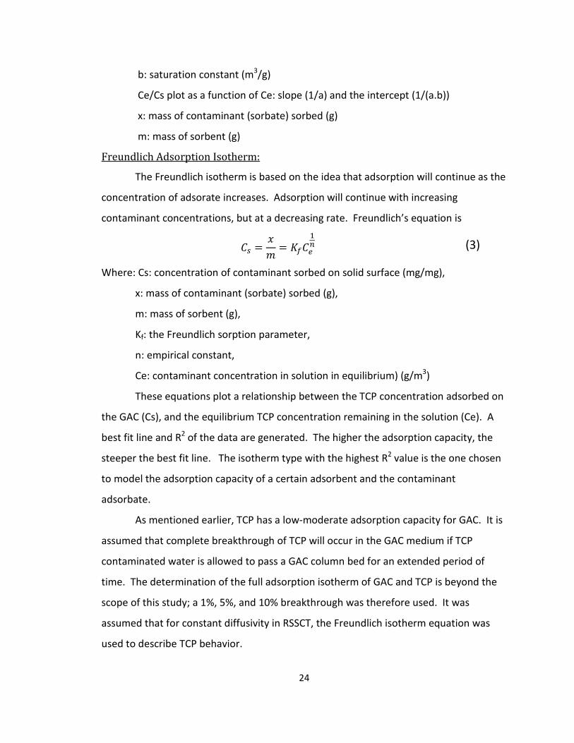
Freundlich Adsorption Isotherm:
The Freundlich isotherm is based on the idea that adsorption will continue as the
concentration of adsorate increases. Adsorption will continue with increasing
contaminant concentrations, but at a decreasing rate. Freundlich’s equation is
𝐶𝑠 =𝑥𝑚
= 𝐾𝑓𝐶𝑒1𝑛 (3)
Where: Cs: concentration of contaminant sorbed on solid surface (mg/mg),
x: mass of contaminant (sorbate) sorbed (g),
m: mass of sorbent (g),
Kf: the Freundlich sorption parameter,
n: empirical constant,
Ce: contaminant concentration in solution in equilibrium) (g/m3)
These equations plot a relationship between the TCP concentration adsorbed on
the GAC (Cs), and the equilibrium TCP concentration remaining in the solution (Ce). A
best fit line and R2 of the data are generated. The higher the adsorption capacity, the
steeper the best fit line. The isotherm type with the highest R2 value is the one chosen
to model the adsorption capacity of a certain adsorbent and the contaminant
adsorbate.
As mentioned earlier, TCP has a low-moderate adsorption capacity for GAC. It is
assumed that complete breakthrough of TCP will occur in the GAC medium if TCP
contaminated water is allowed to pass a GAC column bed for an extended period of
time. The determination of the full adsorption isotherm of GAC and TCP is beyond the
scope of this study; a 1%, 5%, and 10% breakthrough was therefore used. It was
assumed that for constant diffusivity in RSSCT, the Freundlich isotherm equation was
used to describe TCP behavior.
25
Rapid Small Scale Column Test 2.3
Rapid Small-Scale Column Test (RSSCT) was carried out in accordance with the
American Society for Testing and Materials (ASTM) D-6586 – 03(2008) (Materials 2008)
and “Design of Rapid Small-Scale Adsorption Tests for a Constant Diffusivity (Crittenden,
Berrigan et al. 1986).
2.3.1 Approach
RSSCT is a method developed by J.C. Crittenden for the evaluation of GAC for the
adsorption of soluble contamination from water. RSSCT uses the concept of scaling the
hydrodynamics and mass transport of the full-sized GAC in the full-scale column to a
smaller GAC in the small-scale column bench test (Westerhoff 2004). It achieves this
scaling by using dimensionless parameters from the surface diffusion and dispersed-
flow pore model (DFPSDM) (Crittenden, Berrigan et al. 1986, Crittenden, Berrigan et al.
1987), which uses many of the practices that occur in fixed-bed adsorption. DFPSDM
devices cause the breakthrough curves of an adsorber to disperse and create similar
mass transfer zones (MTZ) in the full-scale and small-scale columns, consequently
resulting in similar breakthrough curves. Mechanisms used include axial dispersion and
diffusion, external and internal mass transfer resistance, surface and pore diffusion,
advective flow, and adsorption equilibrium (Crittenden, Berrigan et al. 1986).
The goal is to predict the adsorption of the contaminant onto the GAC in the
actual water treatment plants through the RSSCT. This is achieved by passing the TCP
contaminated water at a constant flow rate through a bed of GAC, testing the effluent
water for the contaminant, and analyzing their breakthrough curves.
Two key assumptions must be made in order for RSSCT to be valid:
1. GAC properties must be the same for full-scale and small-scale test (e.g.,
adsorption capacity, bulk density, porosity).
2. The specified contaminant (TCP) and other compounds completing for
adsorption sites must rely on the particle size in the same way.

26
The four main advantages of the RSSCT are:
1. It requires less time compared to that required by pilot studies.
2. It does not require extensive isotherm or kinetic studies as do some
mathematical prediction models.
3. It does not require a large volume of contaminated water, thus making it
amenable and convenient to carry out experimentally in a laboratory.
4. It is cost efficient compared to other models.
There are two types of commonly used RSSCT design approaches: constant
diffusivity test (CD-RSSCT) and proportional diffusivity test (PD-RSSCT). The CD-RSSCT is
often used for low natural organic matter (NOM) water to predict removal of a specified
contaminant, while PD-RSSCT has been shown to predict removal of NOM and
disinfected byproduct (DBP) (Crittenden, Reddy et al. 1991, Summers, Hooper et al.
1995). It is still uncertain which of the two tests is more appropriate for removal of
trace organic compounds; for this study, however, the constant diffusivity test was
used.
All types of water can be subjected to this procedure, including highly
contaminated water, potable water, wastewater, sanitary wastes, and effluent waters.
2.3.2 Development of Scaling Equations
Six independent dimensionless parameters, Dgs,I, Dgp,I, Eds,I, Edp,I, Pei, and Sti
need to be held constant in order for the full-scale adsorber to be correctly scaled to
the small-scale version. These parameters are defined in Error! Reference source not
found.2 (Fotta 2012) where:
ɛp is the intra-particle porosity, ɛ is the bed porosity, Dp is the pore diffusion coefficient,
t is the fluid residence time in packed bed, dp is the particle diameter, Ds is the surface
diffusivity, CF is the capacity factor, L is the bed length, v is the fluid velocity, Dx is the
dispersion coefficient, kf is the film mass transfer coefficient, q0 is the solid phase
equilibrium concentration, C0 is the influent phase concentration, and ρb is the density.

27
The capacity factor is defined by:
𝐶𝐹 =𝑞0 × 𝜌𝑏𝐶0 × ɛ
(4)
Table 2: Independent Dimensionless Parameters for RSSCT Scaling Process
The intra-particle diffusivity is independent of carbon particle radius, and small-
scale and full-scale models have identical Reynold’s numbers. Thus, the small-scale test
can simulate the specified full-scale model.
To find scaling relationships, some assumptions were made for the following
parameters that affect the GAC performance: backwashing, physical characteristics of
the GAC, adsorption equilibrium capacity, and adsorption kinetics. Changing any of
these parameters could result in poor representation of full-scale performance from
RSSCT.
Backwashing was not used in scaling equations; however, simulation of
backwashing in RSSCT may be possible if GAC particle distribution in RSSCT and full-scale
models are identical. Equilibrium and adsorption capacity are assumed to be identical in
small-scale and full-scale models. Isotherm capacity of RSSCT GAC and unground full-
scale GAC were also identical (Berrigan 1985). The physical characteristics of GAC
(apparent and bulk density and bed void fraction) were not used in scaling equations

28
because studies have shown that they have little impact on performance (Berrigan
1985, Berrigan 1985). Adsorption kinetics, pore and surface diffusion coefficients Ds and
Dp, respectively, have been found to be independent of particle size only when pore and
surface diffusivities in small-scale test were identical to that in the full-scale test
(Dobrzelewski 1985, Crittenden, Berrigan et al. 1986).
Insoluble material such as fats, oils, greases, suspended solids, and emulsions
must be removed before testing starts. These insoluble materials obstruct the
contaminant’s adsorption to the GAC. Air bubbles also must be removed because it
interferes with water flow.
The following equations can describe the relationship between small and large
columns:
𝐸𝐸𝐶𝐸𝑠𝑠𝐸𝐸𝐶𝐸𝑙𝑠
= �𝑅𝑠𝑠𝑅𝑙𝑠
�2
=𝑡𝑠𝑠𝑡𝑙𝑠
(5)
Where: EBCTsc and EBCTlc are the empty bed contact times for the small scale
and full scale column, respectively;
Rsc and Rlc are the carbon particle radii for the small and full scale
column, respectively;
tsc and tlc are the elapsed time required to conduct the small and full
scale test, respectively; and
Vsc and Vlc are the hydraulic loading in the small and large column,
respectively.
In order for equation 2 to be valid, the solute distribution parameters, Dgi, were
assumed to be identical for RSSCT and full-scale tests.
Stanton numbers, Sti, was identical in RSSCT and full-scale tests based on
equation 6 relating liquid-phase mass transfer coefficients which were achieved based
on identical Sherwood numbers. The general equation of liquid-phase mass transfer
29
correlations is shown in equation 7. Determination for film transfer coefficients in
fixed-bed adsorbers was found to be correct (Williamson 1963, E. J. Wilson 1966)
𝑘𝑓,𝑠𝑠
𝑘𝑓,𝑙𝑠=𝑅𝑙𝑠𝑅𝑠𝑠
(6)
𝑆ℎ𝑖 = 𝐹(𝑅𝑅𝑖 ,𝑆𝑆𝑖) (7)
Where: Shi is the Sherwood number and Rei is the Reynolds number.
The hydraulic loading and particle size of full-scale and small-scale tests are
represented by equation 8. This equation guarantees identical Reynolds numbers for
full-scale and small-scale tests.
𝑉𝑠𝑠𝑉𝑙𝑠
=𝑅𝑙𝑠𝑅𝑠𝑠
(8)
Where: Vsc and Vlc are the hydraulic loading in the small and large column
respectively.
It is recommended that the RSSCT be compared to a pilot point column test.
This would help in the selection of the RSSCT design variables and reduce the chance of
calculation mistakes (Crittenden, Berrigan et al. 1986). However, it was not done in this
particular study.
The proper GAC column volume and preparation methods are crucial to the
success of the RSSCT. To avoid channeling of GAC particles, the minimum small scale
GAC column diameter should be 50 particle diameters. In this experiment, all small
scale GACs besides run #11 (mesh size comparison) had mesh sizes of no. 170 X 200
(0.088 by 0.075 mm) which fulfill the minimum column diameter requirement.
Breakthrough curves can be generated based on the water flow rate to the GAC
column, the time each water sample was tested, and the concentration of contaminant
in the effluent water at a specified time.

30
2.3.3 Drawbacks
Compared to pilot point studies, the RSSCT does not have an actively running
evaluation of issues that can affect the GAC performance. These issues include:
• Bacterial colonizing on GAC (Owen, Chowdbury et al. 1996)
• Long term fouling of GAC (Knappe, Snoeyink et al. 1997)
3 METHODS AND PROCEDURES
Water Sample Transport and Preparation 3.1
Raw water samples from each well site were collected in five gallon food grade
polyethylene containers. A total of twenty water containers were used. The samples
were collected directly from the operating well on site. The selected well sites have
multiple individual wells within the site to meet peak flow demand and operational
redundancy. Water was collected on a weekly basis and was transported directly to the
laboratory. Water containers in use were placed into a large refrigerator set at 10˚C and
the remaining containers were stored in a cold room at 4˚C.
Each GAC column was connected to a RSSCT metering pump and used one water
container. This meant that if a run consisted of three GAC columns, then three water
containers were used. This protocol reduces error caused by a GAC column apparatus
malfunction or a failure to replace water. Water containers stored in the cold room
were used to feed containers in the refrigerator as water levels lowered.
To prevent sample contamination, workers were required to wear sterile gloves
during sample collection and extractions in the lab.
Analytical Details 3.2
Water samples from the RSSCT column effluent were designed to be collected in
set time intervals determined by the GAC particle size. However, because different GAC
types (thus, different particle sizes) were run at the same time, the time intervals were
not all at the same. If three different GACs types were run at once, there would be eight

31
sampling times a day. Each sample took between 25 - 70 minutes to collect so this was
an unreasonable task to ask of the 2- 3 workers. Instead, every run was collected three
times per day at 12:00 am, 8:00 am, and 4:00 pm. The length of each run ranged from
14 - 20 days, varying due to water source and carbon type.
The samples were submitted for laboratory analysis by CDPH Modified United
States Environmental Protection Agency Method 524.2 by purge and trap Gas
Chromatography (GC) and Mass Spectrometry (MS). This lab analysis was carried out by
UH-WRRC; however, because UH-WRRC lab is not state certified with the modified EPA
Method 524.2, the samples were also analyzed by BC Laboratories, an environmental
laboratory located in Bakersfield, California, that is state certified to perform the
modified EPA Method 524.2.
Samples were collected in 300 mL BOD bottles for the UH-WRRC lab analysis.
These samples were placed in the 4°C cold room until extraction was carried out.
During extraction, the samples were poured into the 40 mL EPA sample vials (preserved
with HCl) for BC Lab analysis. Each sample was poured into two BC vials to provide
duplicates and enhance accuracy of test. The vials were supplied by BC Labs. In
addition to the tested samples, a travel blank (deionized water) and field blank (influent
water indirectly from water source) were collected and analyzed in both labs.
Samples were analyzed for TCP. EPA Standard Methods were used. TCP was
analyzed by laboratory methods with a detection limit for EPA Method 524.2 of 5 parts
per million (ppt). A brief overview of EPA Method 524.2 is provided in section 3.5.
UH-WRRC quality control included 10% duplicates and 10% continuing
calibration verification. After the initial RSSCT, the need to duplicate the samples to BC
Laboratories was re-evaluated. It was decide that samples would continue to have
duplicates.
Determination of RSSCT Flow Rate 3.3
The governing equations mentioned earlier in section 2.3.2 were the basics of
calculating most RSSCT flow rates.

32
𝐸𝐸𝐶𝐸𝑠𝑠𝐸𝐸𝐶𝐸𝑙𝑠
= �𝑅𝑠𝑠𝑅𝑙𝑠
�2
=𝑡𝑠𝑠𝑡𝑙𝑠
(5)
𝑉𝑠𝑠𝑉𝑙𝑠
=𝑅𝑙𝑠𝑅𝑠𝑠
(8)
In this study, however, because the RSSCT column depth was purposely set at
2.00 cm, equation 8 was not applicable. In order to simplify the study, all RSSCT runs #2
- 10 used the same column depth. However, forcing all of columns to have the same
depth meant that proportions were inconsistent, leading to different full-scale and
small-scale Reynold’s numbers, thus rendering equation 8 invalid.
Other fundamental fluid mechanics and environmental engineering equations
were used. They are shown in appendix 7.1.
The first step was to collect all the known parameters for the full-scale model
and small-scale model. For the full-scale model, the only known parameters were the
GAC weight (WLC), GAC specific gravity (SGLC), flow rate (QLC), column diameter (CDLC),
and US. Sieve No. through which the GAC was sieved. Using these parameters, the
column sectional area (ALC), column volume (VolLC), column depth (LLC), velocity, EBCTLC,
bed-volumes treated, and average GAC particle sizes were calculated.
For the small-scale model, the only known parameters were the column
diameter (CDSC), GAC specific gravity (SGSC), and column depth (LSC). Using these
parameters, the column sectional area (ASC), velocity (VSC), column volume (VolSC),
EBCTSC, bed-volumes treated, GAC mass (mSC), average GAC particle sizes, and flow rate
(QSC) were calculated. The step-by-step calculations are shown in appendix 7.1
The goal of scaling the columns was to determine the small-scale (RSSCT) flow
rates for each GAC size.

33
GAC Properties 3.4
The properties of both small-scale and full-scale models are shown below in
Table 3. Calculations for the column sizing calculations are shown in Appendix 7.1.
Due to a miscommunication between the Primary Investigator and Graduate
Assistant, an earlier version’s (v3) flow rates were used for several GACs at the Kunia I
well source and all GACs at the Waipahu III well source. All six GACs were tested with
version 5’s (v5) flow rates for each water source.
Table 3: Full and Small Scale GAC Properties (v5)
Full - Scale Small - Scale Carbon ID A/B, F, G D, E C A/B, F, G D, E C
Mesh Size US Sieve No.
12x40 (1.68 mm x 0.42 mm)
12x30 (1.68 mm x 0.595 mm)
8x30 (2.38 mm x 0.595 mm)
170x200 (0.088 mm x 0.075 mm)
170x200 (0.088 mm x 0.075 mm)
170x200 (0.088 mm x 0.075 mm)
GAC Avg. Particle Size 1.00 mm 1.14 mm 1.49 mm 0.082 mm 0.082 mm 0.082 mm
Flow Rate v5 3785 m3/d 5.10 mL/min
6.63 mL/min
11.32 mL/min
Flow Rate v3 3785 m3/d 4.35 mL/min
5.66 mL/min
9.67 mL/min
Column Diameter 3.66 m 4.76 mm
Column Depth 2.59 m 2.00 cm
Column Volume 27.2 m3 0.355 mL
EBCT 10.355 min 0.070 min 0.054 min 0.031 min Fill Weight 30000 lbs 0.178 g
3.4.1 RSSCT Test Apparatus
The following equipment and materials were needed to assemble the RSSCT test
apparatus:
• Small-Scale GAC Columns (4)
• 100-mesh stainless screen filters (2 per column, total 8)
• Neoprene O-rings (2 per column, total 8)

34
• Metal threads (2 per column, 8 total)
• PTFE Teflon tape
• Liquid metering pumps with flow rate indicator (4)
• Pressure gauges (4)
• Metal ring stand
• Water sample collection BOD bottles (1 per sample)
• Thin transparent tubing (size not specified)
• Oven
• Refrigerator (set at 10˚ C)
• Extraction Set – Up
• Effluent Containers (6)
• Analytical Balance
• Data Log Book
A photograph of the actual RSSCT test apparatus is shown in Figure 13.

35
Figure 13: Actual RSSCT Test Apparatus

36
Each component of the test apparatus is described in the following figures.
1. Small-Scale GAC Columns – The columns, shown in Figure 14, has a GAC column
bed of 4.76 mm diameter x 2.00 cm deep column bed. Figure 15 shows a
loaded GAC column actively in use.
Figure 14: Small Scale GAC Column
Figure 15: GAC Column During a Run

37
2. GAC Supports – Metal threads are used to provide a sealed connection between the
tubing and the glass column. Prior to twisting the metal thread into the column, a
100-mesh stainless screen is placed into the column to prevent GAC from leaking
out, and PTFE (Teflon tape) is wrapped around the metal threads and a neoprene O-
ring is placed into the column to provide a further water seal. Metal threads are
shown below in Figure 16.
Figure 16: Metal Threads
3. Liquid Metering Pumps – A pump capable of maintaining a steady flow rate of
±0.05 mL/min at a column back pressure up to 100 psi was used. The pump has
a bypass loop to allow the flow from the pump to recirculate to the pump inlet
to relief pressure caused in the pump system. The pressure and water flow rate
should be monitored and recorded in the data log book at each sample
collection. Figure 17 shows the water pumps.

38
Figure 17: Liquid Metering Pumps
4. Pressure Gauges – Pressure gauges were used to monitor the pressure in each
system. They were attached to the tubing between the water pump outlet and
the GAC column inlet. Figure 18 below shows the pressure gauge used in this
test.
Figure 18: Pressure Gauge
5. Water Filtration – Water filtration was not used in the experiment.

39
6. Water Containment – The water being treated should be held at the same
constant temperature as the GAC columns. The plastic containers containing the
well water were held in a refrigerator at 10˚C. Tubing connected to the water
pumps were inserted into the plastic container to pump the water out. Holes
were cut in the refrigerator openings to provide space for the tube to enter the
refrigerator. Plastic funnels were used to assist in the pouring of water into the
containers. Since TCP is a volatile organic compound (VOC), it was important
that all water containers containing the influent water be properly capped.
During the pumping from the water container, however, the tube used to deliver
water obstructed appropriate capping of the container. The container was
therefore capped in such a way as to minimize the exposure of the water to the
outside air as shown below in Figure 19.
Figure 19: Water Containers

40
7. Sample Collection System –300 mL BOD bottles were used to collect effluent
water samples on a timely basis with zero head-space. The collected samples
were stored in a refrigerated area to preserve the integrity of the sample.
Samples can be collected in 35 mL vials up to 2 L water containers depending on
the type of analysis performed. It should be noted that low flow rates and large
water sample containers will contribute to sampling collection over an extended
period of time. Error! Reference source not found. shows the BOD bottles used
for water sample collection.
Figure 20: Effluent Water Samples
8. Sample Analysis – Auto-sampler vials were used to collect the extracted samples.
These vials were subject to TCP analysis. When RSSCT was done for an extended
period of time, the most recent samples were extracted and analyzed first in the
reverse order from which it was sampled. Once several samples showed no
breakthrough, the earlier samples did not need to be extracted and analyzed,
thus saving time. Figure 21 shows an auto-sampler vial.
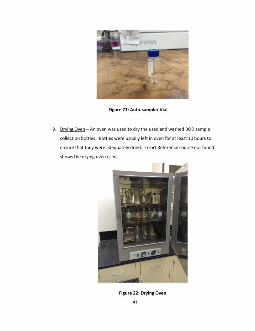
41
Figure 21: Auto-sampler Vial
9. Drying Oven – An oven was used to dry the used and washed BOD sample
collection bottles. Bottles were usually left in oven for at least 10 hours to
ensure that they were adequately dried. Error! Reference source not found.
shows the drying oven used.
Figure 22: Drying Oven

42
10. Refrigerator – The water containers in use were placed in a refrigerator to
maintain a constant temperature. The refrigerator could store up to 8 water
containers. Figure 23 below shows the refrigerator used.
c
Figure 23: Refrigerator
11. Extraction Set -Up – Extraction of the contaminant (TCP) was a subsection of the
RSSCT procedure. It was not specified in RSSCT how extraction should be

43
conducted. The extraction in this study was developed by the UH-WRRC staff to
serve as an effective means of pulling out the contaminant from the water
sample so that its concentration could be analyzed. The extraction set-up is
shown in Figure 24.
Figure 24: Extraction Set-Up
12. Effluent containers – Effluent containers were used to collect the effluent water
in between sampling times. This effluent water was used to determine the
actual flow rate in the system. The flow rates displayed on the water pumps

44
were slightly different from the actual; the water pumps flow rates were
therefore adjusted according to the actual flow rate being discharged. Figure 25
below shows each GAC’s effluent water containers.
Figure 25: Effluent Containers

45
13. Data Log Book – A data log book was used to record the sample name, date,
time, etc. for each sample. Proper and neatly recorded data was essential to the
success of this study. The data log book is shown in Figure 26
Figure 26: Data Log Book
46
3.4.2 Reagents
• Granular Activated Carbon (GAC)
• Well water source
3.4.3 Experimental Procedures
Since UH-WRRC lab only has four water pumps, only four GAC columns could be
run at once. There are six GACs being tested; two runs, therefore, were required per
well. After each completed run, the RSSCT equipment was dismantled, cleaned, and
reassembled for the next run. Each run took approximately 2 weeks; it varied, however,
between each GAC type and well sources. The higher the influent TCP concentration,
the earlier the run was terminated. A run was only required to reach 10% of its influent
TCP concentration (10% breakthrough) before termination. However, some GACs were
stopped before 10% breakthrough because there was not enough time to reach this
level without going over the scheduled end date of this project. Values for these
occasions were interpolated. This should be taken into account when analyzing the
data.
The experimental procedures that follow were formulated by the UH-WRRC staff.
3.4.4 GAC Grinding and Screening Procedure
A. Dry Sieve Portion
1. The granular activated carbon type to be ground was selected.
2. All carbon grinding was done under a fume hood. A 200 mL sample of selected
GAC was ground using a grinder. Two types of grinders were used: a coffee
grinder and a blender.
3. The GAC was ground for 10-15 seconds in the coffee grinder. After
approximately 30 seconds, the GAC settled and the grinder could be removed.
4. A sieve-stack containing a pan, #200 sieves, #170 sieve, and cover was
assembled. The parts were assembled from bottom to top in the precedent
order.
5. The ground-up GAC was poured into the sieve-stack.

47
6. The sieve-stack was manually shaken for approximately 1 minute.
7. The GAC that had passed the #170 sieve but was retained by the #200 sieve was
poured into a large Ziploc bag.
8. The sieve screens were tapped to make sure the screens were clean and no
carbon remained to clog the sieve openings.
9. The GAC retained at #170 was poured back into the coffee grinder
10. Steps #3 - #9 were repeated two more times and poured into the same Ziploc
bag. The ground-up GAC was then put through a wet sieve.
B. Wet Sieve Portion
1. Deionized (DI) water was poured into the Ziploc bag containing the dry sieved
GAC.
2. The bag was shaken until all the GAC appeared to be wet.
3. The wet GAC was poured out of the bag and into a dry #200 sieve located over a
sink.
4. Deionized water was poured and squirted onto the wet GAC until only a small
amount of GAC was seen passing through the #200 sieve. This was checked by
placing a white crucible under the sieve. Once the water was nearly all clear, the
next step could be continued. However until this happened, this step was
repeated.
5. The wet GAC was poured and squirted into a dry and clean crucible.
6. DI water was squirted into the crucible, mixing the water and GAC.
7. The DI water in the crucible was poured out into the sink along with the top
floating GAC particles. The cleaned GAC was retained in the crucible.
8. Steps #16 - #17 were repeated until floating particles were negligible (5-10
times).
9. The GAC-containing crucible was labeled and placed in the oven until the
crucible was dry.
48
C. GAC Column Loading and Set Up
1. The GAC Column was labeled according to the name of GAC placed in the
column.
2. Two 100-mesh stainless screen filters were cut into circles the size of the column
diameter openings. One filter was placed into the column opening.
3. A rubber O-ring was placed into the column opening onto the filter.
4. A metal thread was wrapped 5 times with Teflon tape.
5. A drop of distilled water was placed on the tip of the thread before it was
screwed into the column. Thread was screwed in until it formed a snug fit to the
O-ring.
6. Approximately 0.178 g of GAC was weighed on an analytical scale and poured
into the column opening. Since all GACs are of different densities, the mass
required to fill the entire column volume varied. It is important that the entire
column volume be filled.
7. The other screen filter was placed in the open column opening onto the GAC
bed.
8. Another rubber O-ring was placed into the open column opening onto the filter.
9. Another metal thread was wrapped 5 times with Teflon tape.
10. A drop of distilled water was placed on the tip of the thread before it was
screwed into the column. Thread was screwed in until it formed a snug fit to the
O-ring. This completed the GAC column loading.
11. The loaded GAC column was clamped to the metal ring stand shown in Figure 13.
12. Repeat steps #2 - #11 for each GAC being tested.
D. Column Testing Procedure
1. The tested water flows through the GAC apparatus via a thin Teflon tubing. This
tubing starts in the water source, connects to the pumps, to the pressure gauge,
to the GAC column, and out through the effluent tube end. Proper set up of this
apparatus system is crucial to the accuracy of the test.

49
2. The tubing was cut into pieces suitable for each tubing connection.
3. Influent tubing was zip tied to a BOD bottle stopper and placed into the water
container containing the influent water. The stopper was tied on the tubing to
ensure the tube would sink to the bottom of the container even as water levels
lowered. This tubing was attached to the pump entrance. Plastic fittings were
used at each connection to make sure there was no leakage.
4. Tubing was connected between the pump exit to the pressure gauge entrance,
from the pressure gauge exit to the column entrance, and from the column exit
to an effluent waste container.
5. The apparatus was checked to ensure that there were no points of leakage.
6. The pump flow rate was set to the desired flow rate.
7. The pump was turned on.
8. The water samples were collected from the effluent tube in 300 mL BOD bottles
until the water reached the neck of the BOD bottle. The sample number and
starting time for each sample were recorded in the data log book. Bottles were
capped, labeled, and placed into the cooling room until extractions were carried
out. Bottles were capped with a stopper to ensure a water-tight seal. Bottles
were labeled with the water source, carbon type, and sample number.
9. Effluent water was collected in the effluent containers and weighed between
sampling intervals. The mass of water was converted to a volume and divided by
the time to determine the actual pumping flow rate, Qa. Qa was recorded to
determine the bed-volumes of water treated. Qa was compared to the pumping
rate shown on the pump, Qp, and adjustments were made accordingly.
10. Water in actively used water containers were checked daily to ensure that the
water levels did not run below ½ filled; if they were, they were filled with the
stored water.
11. If any malfunction or error was found within the system, the pumps were
stopped and their times and the malfunction descriptions were noted. Once the
problem was solved, the pumps were started and their times were again noted.

50
EDB, DBCP, and TCP in Water by Microextraction and Gas 3.5
Chromatography – EPA Method 504.1
TCP analysis was carried out in accordance with the Environmental Protection
Agency (EPA) Method 504.1 – 1,2-Dibromoethane (EDB), 1,2-Dibromo-3-Chloro-propane
(DBCP), and 1,2,3 – Trichloropropane (123TCP) in Water by Microextraction and Gas
Chromatography (EPA 1995). A brief overview of EPA method 504.1’s procedure, data
analysis, and calculations are provided below.
3.5.1 Approach
This procedure is applicable for the determination of TCP in drinking water and
groundwater (Henderson, Peyton et al. 1976, Richard and Junk 1977, Glaze and Lin
1984). Definite detection limits are highly variable on the Gas Chromatography (GC)
used. Hexane was used as a solvent in the TCP extraction process. The 2-mL hexane
extract (explained in section 3.5.3) was injected into the GC. This GC is equipped with a
linearized electron capture detector able to separate and detect the amount of TCP.
Extraction and analysis take approximately 30 – 50 minutes per sample. Evidence
should be acquired for positive results.
3.5.2 Assumptions
The majority of analytical error will be attributed to impurities in the extracting
solvent.
3.5.3 Procedure
Sample Preparation
1. Take samples and standards out from storage and allow them to reach room
temperature before use.
2. For sample and field reagent blanks contained in 40 mL bottles, take off the cap
and extract 5 mL of volume solution. Recap and weigh the bottle to the nearest
0.1 g. This will represent the gross weight, used in the subsequent sample
volume equation (equation 3)

51
Extraction Procedure
1. Protective eye wear, a lab coat, gloves, and shoes were worn for this procedure.
2. Water samples stored in BOD bottles in the cold room were brought out to the
lab bench.
3. Before extraction, each water sample was poured into two 40 mL BC lab vial
containers. The vials were labeled with its corresponding water source, date and
time, and sample number. These vials were given to AECOM, who then sent
them to BC Laboratories to get the samples double checked for TCP analysis.
4. An important note for the extraction procedure is that all separatory funnels,
graduated cylinders, and anything coming in contact with the water sample need
to be washed thoroughly with deionized (DI) water in between samples to avoid
cross contamination. Since there is only an incremental amount of TCP in each
sample, any contamination will have a significant impact on the results.
5. The following items are added to the separatory funnel:
a. 200 mL water sample
b. 35 - 40 grams NaCl
c. 2.0 mL Hexane
6. The separatory funnel was capped with a stopper and shaken vigorously for 1 - 2
minutes.
7. After 1- 2 minutes, layers in the funnel became separated. Two layers formed: a
water layer and a hexane layer. The denser water layer will sit below the less
dense hexane layer.
8. The stopper was removed and the water layer was drained into a waste
container.
9. The hexane layer was drained through a pipette containing sodium sulfide into a
2- mL auto-sampler vial. The sodium sulfide was used to remove any residual
water.
10. The auto-sampler vial was checked again for water. If water was present, it was
extracted with a pipette.
52
11. Vials were labeled and analyzed for TCP using a gas chromatogram (GC). Any
water in these vials could cause the GC machine to malfunction.
Determination of Sample Volume
1. For samples and field blanks, uncap and discard the remaining sample. Make
sure all or as much as possible of the remaining water is removed.
2. Recap the empty container and weigh to the nearest 0.1 g. This represents the
tare weight used in equation 3.
Data Analysis and Calculations
1. Calculate the sample volume (Vs)
𝑉𝑠 = 𝑔𝑔𝑔𝑔𝑔 𝑤𝑅𝑤𝑔ℎ𝑡 − 𝑡𝑎𝑔𝑅 𝑤𝑅𝑤𝑔ℎ𝑡 (10)
2. Calculate the corrected sample concentration as:
𝐶𝑔𝐶𝑆𝑅𝐶𝑡𝑔𝑎𝑡𝑤𝑔𝐶 (𝑝𝑝𝑎) = 𝐶𝑖 ×35𝑉𝑠
(11)
Where: Ci = uncorrected concentration (see EPA Method 504.1 for use of calibration curve)
For concentrations greater than 99 ppb, 3 significant figures were used; for
concentrations from 1 - 99 ppb, 2 significant figures were used; and for less than 1 ppb,
1 significant figure was used.

53
4 RESULTS AND ANALYSIS General 4.1
4.1.1 Results
The results of each of the GACs tested are shown in the following sections. The
bed-volumes treated and TCP mass absorbed per GAC unit at the 1%, 5%, and 10%
breakthrough points are displayed in separate tables. Along with the bed-volumes
treated and TCP mass absorbed, these tables included the GAC type, water source, flow
rate, version, and run number. The tables were color coded to make the results easier
to interpret. Table 4 indicates what each color means.
The breakthrough curves for each water source tested were plotted and are
shown in the figures. The results by GAC type were plotted in relative concentration
instead of effluent TCP concentration so that all water well sources with different
influent TCP concentrations could be compared to one another. Influent TCP
concentrations from each test run with their corresponding breakthrough TCP
concentrations are shown in Table 5. The results by water well source are shown in
effluent TCP concentration instead of relative concentration. Using the effluent TCP
concentrations are very useful because the bed-volumes treated to reach a specific TCP
concentration can be determined.
The results of each GAC were separated into subsections. First, it was
categorized by GAC types as shown in Section 4.2. Each GAC type was tested with the
three water sources. Next, the results are categorized by water well source as shown in
Section 4.4. Each water well source had the six GAC types tested.
Waipahu III and Kunia I-wrong were plotted and shown in the tables; however,
because they are not proportioned correctly, they were not used in the comparative
analysis and not included in the averages. They were used only for a visual
representation of how the GAC might behave at a slightly different flow rate. However,
Kunia I-wrong and Waipahu III v3 can serve as good indicators to see if the breakthrough
curves are following the correct trend. Kunia I-wrong uses a GAC F flow rate of 6.63
mL/min which is larger than the correct GAC F flow rate of 5.10 mL/min. Since

54
everything else is left constant, an increase in flow rate will theoretically yield less bed-
volumes treated at each breakthrough point. Waipahu III v3 has flow rates smaller than
the correct v5 flow rates so it theoretically would yield more bed-volumes treated at
each breakthrough point.
Table 4: Color Interpretation for Result Tables
Color Meaning Light Red GAC Type Yellowish Green Parameters Light Blue Water Well Sources Gray Invalid Results Light Orange Breakthrough Limit Averages Orange Projected Values
Table 5: Influent TCP Concentration with Corresponding Breakthrough Limits
Influent TCP Concentration with Corresponding Breakthrough Limits (ppb)
Run # Water Source Influent Concentration (ppb)
1% Breakthrough (ppb)
5% Breakthrough (ppb)
10% Breakthrough (ppb)
2 Kunia I 0.818 0.0082 0.0409 0.0818 3 Kunia I 0.794 0.0079 0.0397 0.0794 4 Waipahu III 0.554 0.0064 0.0321 0.0641 5 Waipahu III 0.554 0.0055 0.0277 0.0554 6 Mililani I 2.146 0.0215 0.1073 0.2146 7 Mililani I 2.298 0.0230 0.1149 0.2298 8 Kunia I 0.803 0.0080 0.0401 0.0803 9 Waipahu III 0.634 0.0063 0.0317 0.0634
10 Waipahu III 0.634 0.0063 0.0317 0.0634 11 Waipahu III 0.506 0.0051 0.0253 0.0506
4.1.2 Analysis
Theoretically, if the GAC type and flow rate remain constant and everything else
remains the same, the TCP breakthrough curves should be identical. However, there are
many variables to consider that can affect the accuracy of this test.
The initial 1% breakthrough is highly variable because the smallest indication of
TCP concentration will be perceived as an initial breakthrough. However, a small
contamination of the water sample from collection or extraction can be the cause of a

55
false positive 1% breakthrough. A better indication of breakthrough is to measure the
bed-volumes treated at 5% and 10% breakthrough.
Also, there are many other contaminants present in the groundwater tested.
These contaminants such as natural organic matter (NOM) and other volatile organic
compounds (VOC) can be present in groundwater at concentrations magnitudes larger
than of TCP. These other contaminants bind to the GAC surface and can compete for
adsorption sites on the GAC which can affect the GACs adsorption capacity for TCP.
Only TCP was tested for in this study so it is unknown what other contaminants were
present in the groundwater.
Also, two other main compounds, Dibromoethane (EDB) and 1,2-Dibromo-3-
chloropropane (DBCP), which are usually tested for in drinking water were not tested in
this study. The GAC effectiveness to these two other compounds may or may not follow
the same trend as for TCP removal. The selection of the GAC type would normally
depend on which is the most effective at removal of all hazardous compounds instead
of one specific contaminant.

56
Results/Analysis by GAC Type 4.2
4.2.1 GAC A/B Results
Table 6: GAC A/B Breakthrough Results – Bed-Volumes Treated
GAC A/B – Bed-Volumes Treated Well Flow Rate (mL/min) Version Run # 1% Breakthrough 5% Breakthrough 10% Breakthrough Kunia I 5.10 v5 3 161,229 196,004 219,659 Mililani I 5.10 v5 6 158,003 205,508 230,412 Waipahu III 5.10 v5 9 102,778 160,689 201,499 Waipahu III 4.35 v3 5 238,763 296,847 344,999
Average 140,670 187,400 217,190
Table 7: GAC A/B Breakthrough Results – TCP Mass Adsorbed per GAC Unit
GAC A/B – TCP Mass Adsorbed per GAC Unit (mg) Well Flow Rate (mL/min) Version Run # 1% Breakthrough 5% Breakthrough 10% Breakthrough Kunia I 5.10 v5 3 3.48 4.20 4.67 Mililani I 5.10 v5 6 9.21 11.90 13.23 Waipahu III 5.10 v5 9 1.77 2.74 3.39 Waipahu III 4.35 v3 5 3.60 4.45 5.12
Average 4.82 6.28 7.10
Figure 27: GAC A/B Breakthrough Results
0.000
0.010
0.020
0.030
0.040
0.050
0.060
0.070
0.080
0.090
0.100
0.110
0 50000 100000 150000 200000 250000 300000 350000
Rela
tive
Conc
entr
atio
n, C
/Co
Bed-volumes
TCP Breakthrough Curve - GAC A/B
Kunia I - v5
Waipahu III - v3
Waipahu III - v5
Mililani I - v5
57
4.2.2 GAC A/B Analysis
The breakthrough curve for GAC A/B, as shown in Figure 27, shows a similar
breakthrough pattern in Kunia I and Mililani I waters. Waipahu III v5 treated less bed-
volumes than Kunia I and Mililani I while Waipahu III v3 treated a lot more. The
Waipahu III v3 breakthrough curve was approximately 50% greater than the other water
sources at 1%, 5%, and 10% breakthrough. It would make sense that the Waipahu III
water had a different breakthrough curve from the other water sources because the
flow rate used for it was incorrect. The change from 5.10 to 4.35 mL/min would yield
more treated bed-volumes compared to the others, but it would not lead to that drastic
of an increase. Again all Waipahu III v3 results were not used in averages or GAC type
comparisons. It was thought that the breakthrough curves for the different water well
sources would be the same, but it was seen that Kunia I was not the same as the other
two. This means that there must be something different amongst the different water
sources that are affecting how the TCP is being adsorbed to the GAC. The water matrix
of each water source must contain different concentrations of other contaminants.
As shown in Table 6, the 1%, 5%, and 10% breakthrough average bed-volumes
treated were 140670, 187400, and 217190 respectively. As shown in
Table 7, TCP mass adsorbed was not the same for the different water sources.
Mililani I water showed the most TCP adsorbed. The 1%, 5%, and 10% breakthrough
average TCP adsorbed were 4.82, 6.28, and 7.10 mg, respectively.

58
4.2.3 GAC C Results
Table 8: GAC C Breakthrough Results – Bed-Volumes Treated
GAC C – Bed-Volumes Treated Well Flow Rate (mL/min) Version Run # 1% Breakthrough 5% Breakthrough 10% Breakthrough Kunia I 11.32 v5 2 51,230 97,142 113,325 Mililani I 11.32 v5 6 26,395 71,843 103,852 Waipahu III 11.32 v5 10 35,212 67,711 91,732 Waipahu III 9.67 v3 5 65,147 109,268 128,116
Average 37,612 78,899 102,969
Table 9: GAC C Breakthrough Results – TCP Mass Adsorbed per GAC Unit
GAC C – TCP Mass Adsorbed per GAC Unit (mg) Well Flow Rate (mL/min) Version Run # 1% Breakthrough 5% Breakthrough 10% Breakthrough Kunia I 11.32 v5 2 0.49 0.93 1.07 Mililani I 11.32 v5 6 1.53 4.09 5.80 Waipahu III 11.32 v5 10 0.60 1.14 1.52 Waipahu III 9.67 v3 5 0.98 1.63 1.89
Average 0.88 2.05 2.80
Figure 28: GAC C Breakthrough Results
0
0.01
0.02
0.03
0.04
0.05
0.06
0.07
0.08
0.09
0.1
0.11
0 50000 100000 150000 200000 250000 300000 350000
Rela
tive
Conc
entr
atio
n, C
/Co
Bed-volumes
TCP Breakthrough Curve - GAC C
Kunia I - v5
Waipahu III - v3
Waipahu III - v5
Mililani I - v5

59
4.2.4 GAC C Analysis
The breakthrough curve for GAC C, as shown in
Figure 28, shows a similar breakthrough pattern in all the waters tested. Waipahu III v5
and Mililani I showed nearly identical breakthrough curves, while Kunia I and Waipahu
III v3 treated slightly more bed-volumes. The Mililani I water was the first to show an
initial breakthrough (1% breakthrough) at 26395 bed-volumes while the Kunia I water
was the last at 51230 bed-volumes. The 5% breakthroughs were relatively precise
ranging from 67711 to 97142 bed-volumes. The 10% breakthroughs were also relatively
precise ranging from 91732 to 113325 bed-volumes. GAC C, the current GAC used in
Hawaii’s water treatment facilities made of Jacobi direct-activated coal based carbon
8x30, was seen to treat the least bed-volumes at each breakthrough point. Their bed-
volumes treated were substantially lower than the other GACs values. Because of this,
consideration should be taken to replace it with another GAC.
As shown in Table 8, the 1%, 5%, and 10% breakthrough average bed-volumes
treated were 37612, 78899, and 102696, respectively. As shown in
Table 7, TCP adsorbed was not the same for the different water sources. Mililani
I water showed the most TCP adsorbed. The 1%, 5%, and 10% breakthrough average
TCP adsorbed were 0.88, 2.05, and 2.80 mg, respectively.
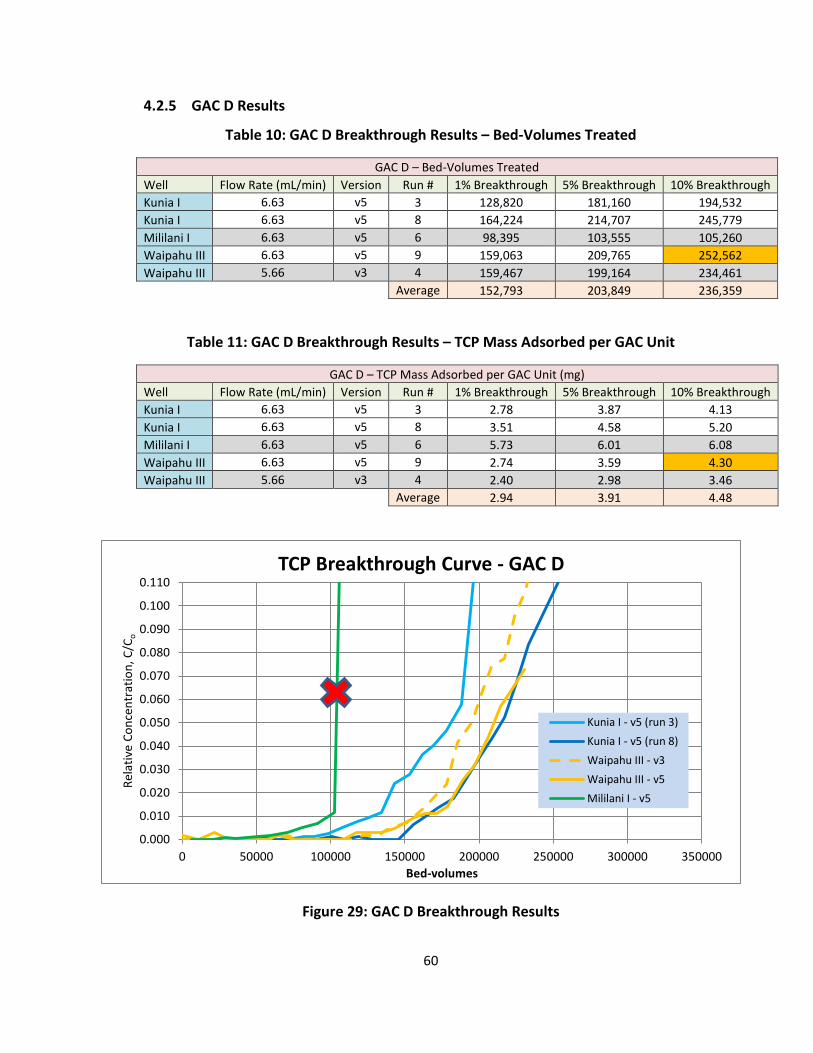
60
4.2.5 GAC D Results
Table 10: GAC D Breakthrough Results – Bed-Volumes Treated
GAC D – Bed-Volumes Treated Well Flow Rate (mL/min) Version Run # 1% Breakthrough 5% Breakthrough 10% Breakthrough Kunia I 6.63 v5 3 128,820 181,160 194,532 Kunia I 6.63 v5 8 164,224 214,707 245,779 Mililani I 6.63 v5 6 98,395 103,555 105,260 Waipahu III 6.63 v5 9 159,063 209,765 252,562 Waipahu III 5.66 v3 4 159,467 199,164 234,461
Average 152,793 203,849 236,359
Table 11: GAC D Breakthrough Results – TCP Mass Adsorbed per GAC Unit
GAC D – TCP Mass Adsorbed per GAC Unit (mg) Well Flow Rate (mL/min) Version Run # 1% Breakthrough 5% Breakthrough 10% Breakthrough Kunia I 6.63 v5 3 2.78 3.87 4.13 Kunia I 6.63 v5 8 3.51 4.58 5.20 Mililani I 6.63 v5 6 5.73 6.01 6.08 Waipahu III 6.63 v5 9 2.74 3.59 4.30 Waipahu III 5.66 v3 4 2.40 2.98 3.46
Average 2.94 3.91 4.48
Figure 29: GAC D Breakthrough Results
0.000
0.010
0.020
0.030
0.040
0.050
0.060
0.070
0.080
0.090
0.100
0.110
0 50000 100000 150000 200000 250000 300000 350000
Rela
tive
Conc
entr
atio
n, C
/Co
Bed-volumes
TCP Breakthrough Curve - GAC D
Kunia I - v5 (run 3)Kunia I - v5 (run 8)Waipahu III - v3Waipahu III - v5Mililani I - v5

61
4.2.6 GAC D Analysis
The breakthrough curves for GAC D, as shown in Figure 29, show a similar
breakthrough pattern in all the waters tested except Mililani I and Kunia I – v5 (run 3).
The Mililani I samples were subjected to a source of error. The TCP concentration in
Mililani I samples jumped from 0.247 to 1.103 ppb (C/Co equivalent jump of 0.115 to
0.514) over less than an 8 hour time span. These samples were inadvertently exposed
to the air for about 10 hours, during which time it was highly possible that the TCP
contaminant partially evaporated. It is highly unlikely that the TCP concentration would
jump that drastically in such a small time interval. The Mililani I results were omitted
from statistical analysis. The Kunia I samples were accidentally run twice at the exact
same flow rate. This is the only GAC in the experiment that was rerun at the same flow
rate. Theoretically, the breakthrough curves should be identical, but it can be seen that
this is not the case. Kunia I – v5 (run #3) treated less bed-volumes at each breakthrough
point when compared to run #8. The average of these two runs was used.
As shown in Table 10, the 1%, 5%, and 10% breakthrough average bed-volumes
treated were 152793, 203849, and 236359, respectively. As shown in Table 11, TCP
adsorbed was relatively similar for the two valid water sources. The 1%, 5%, and 10%
breakthrough average TCP adsorbed were 2.94, 3.91, and 4.48 mg, respectively.
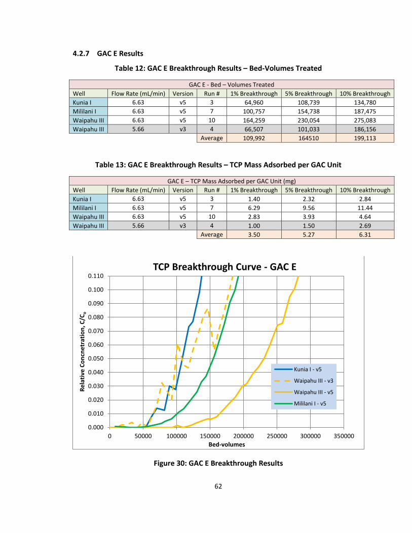
62
4.2.7 GAC E Results
Table 12: GAC E Breakthrough Results – Bed-Volumes Treated
GAC E - Bed – Volumes Treated Well Flow Rate (mL/min) Version Run # 1% Breakthrough 5% Breakthrough 10% Breakthrough Kunia I 6.63 v5 3 64,960 108,739 134,780 Mililani I 6.63 v5 7 100,757 154,738 187,475 Waipahu III 6.63 v5 10 164,259 230,054 275,083 Waipahu III 5.66 v3 4 66,507 101,033 186,156
Average 109,992 164510 199,113
Table 13: GAC E Breakthrough Results – TCP Mass Adsorbed per GAC Unit
GAC E – TCP Mass Adsorbed per GAC Unit (mg) Well Flow Rate (mL/min) Version Run # 1% Breakthrough 5% Breakthrough 10% Breakthrough Kunia I 6.63 v5 3 1.40 2.32 2.84 Mililani I 6.63 v5 7 6.29 9.56 11.44 Waipahu III 6.63 v5 10 2.83 3.93 4.64 Waipahu III 5.66 v3 4 1.00 1.50 2.69
Average 3.50 5.27 6.31
Figure 30: GAC E Breakthrough Results
0.000
0.010
0.020
0.030
0.040
0.050
0.060
0.070
0.080
0.090
0.100
0.110
0 50000 100000 150000 200000 250000 300000 350000
Rela
tive
Conc
netr
atio
n, C
/Co
Bed-volumes
TCP Breakthrough Curve - GAC E
Kunia I - v5
Waipahu III - v3
Waipahu III - v5
Mililani I - v5

63
4.2.8 GAC E Analysis
The breakthrough curves for GAC E, as shown in Figure 30, show breakthrough
curves from each water well source that are all not very similar, with Waipahu III v5
treating a lot more bed-volumes than the rest. The Waipahu III v5 samples showed bed-
volumes at each breakthrough limits that were over 50% greater than the next highest
water source. The Kunia I and Waipahu III v3 breakthrough curves showed very similar
1% breakthroughs, however, once again, Waipahu III v3 cannot be used for in the
analysis process. Therefore, Kunia I showed the lowest breakthrough values of the valid
water samples for each of the 1%, 5%, and 10% breakthrough points.
As shown in Table 12, the 1%, 5%, and 10% breakthrough average bed-volumes
treated were 109992, 164510, and 199113, respectively. As shown in Table 13, TCP
mass adsorbed was not the same for the different water sources. Mililani I water
showed the most TCP adsorbed. The 1%, 5%, and 10% breakthrough average TCP
adsorbed were 3.50, 5.27, and 6.31 mg, respectively.

64
4.2.9 GAC F Results
Table 14: GAC F Breakthrough Results – Bed-Volumes Treated
GAC F – Bed-Volumes Treated Well Flow Rate (mL/min) Version Run # 1% Breakthrough 5% Breakthrough 10% Breakthrough Kunia I 5.10 v5 8 90,183 135,942 161,667 Kunia I 6.63 Wrong 3 56,787 106,151 137,539 Mililani I 5.10 v5 7 126,272 171,791 206,858 Waipahu III 5.10 v5 9 122,887 184,938 218,307 Waipahu III 4.35 v3 4 132,957 183,896 218,547
Average 113,114 164,223 195,610
Table 15: GAC F Breakthrough Results – TCP Mass Adsorbed per GAC Unit
GAC F – TCP Mass Adsorbed per GAC Unit (mg) Well Flow Rate (mL/min) Version Run # 1% Breakthrough 5% Breakthrough 10% Breakthrough Kunia I 5.10 v5 8 1.96 2.93 3.45 Kunia I 6.63 Wrong 3 1.22 2.25 2.88 Mililani I 5.10 v5 7 7.88 10.65 12.63 Waipahu III 5.10 v5 9 2.11 3.16 3.68 Waipahu III 4.35 v3 4 2.00 2.74 3.21
Average 3.99 5.58 6.59
Figure 31: GAC F Breakthrough Results
0.000
0.010
0.020
0.030
0.040
0.050
0.060
0.070
0.080
0.090
0.100
0.110
0 50000 100000 150000 200000 250000 300000 350000
Rela
tive
Conc
entr
atio
n. C
/Co
Bed-volumes
TCP Breakthrough Curve - GAC F
Kunia I - wrong
Kunia I - v5
Waipahu III - v3
Waipahu III - v5
Mililani I - v5

65
4.2.10 GAC F Analysis
The breakthrough curves for GAC F, as shown in Figure 31, show nearly identical
breakthrough curves in the Waipahu III v3, Waipahu III v5, and Mililani I sources. Both
of the Kunia I wrong and v5 water treated less bed-volumes than the other three water
sources. The Kunia I wrong water had breakthrough values smaller than the Kunia I v5
water which makes sense based on the statement in section 4.1.1. Again, Kunia I wrong
and Waipahu III v3 breakthrough curves cannot be used.
As shown in Table 14, the 1%, 5%, and 10% breakthrough average bed-volumes
treated were 113114, 164223, and 195610, respectively. As shown in Table 15, TCP
mass adsorbed was similar for Kunia I and Waipahu II v5, but Mililani was higher than
those. The 1%, 5%, and 10% breakthrough average TCP adsorbed were 3.99, 5.58, and
6.59 mg, respectively.

66
4.2.11 GAC G Results
Table 16: GAC G Breakthrough Results – Bed-Volumes Treated
GAC G – Bed-Volumes Treated
Well Flow Rate (mL/min) Version Run # 1% Breakthrough 5% Breakthrough
10% Breakthrough
Kunia I 5.10 v5 8 55465 100,264 150,391 Mililani I 5.10 v5 7 121,200 170,807 197,542 Waipahu III 5.10 v5 10 164,259 230,054 275,083 Waipahu III 4.35 v3 5 174,595 219,551 258,980
Average 113,641 170,375 207,674
Table 17: GAC G Breakthrough Results – TCP Adsorbed per GAC Mass
GAC G – TCP Mass Adsorbed per GAC Unit (mg)
Well Flow Rate (mL/min) Version Run # 1% Breakthrough 5% Breakthrough 10%
Breakthrough Kunia I 5.10 v5 8 1.20 2.15 3.17 Mililani I 5.10 v5 7 7.80 10.34 11.88 Waipahu III 5.10 v5 10 2.83 3.93 4.64 Waipahu III 4.35 v3 5 2.63 3.28 3.83
Average 3.95 5.47 6.56
Figure 32: GAC G Breakthrough Results
0.000
0.010
0.020
0.030
0.040
0.050
0.060
0.070
0.080
0.090
0.100
0.110
0 50000 100000 150000 200000 250000 300000 350000
Rela
tiive
Con
cent
ratio
n. C
/Co
Bed-volumes
TCP Breakthrough Curve - GAC G
Kunia I - v5
Waipahu III - v3
Waipahu III - v5
Mililani I - v5
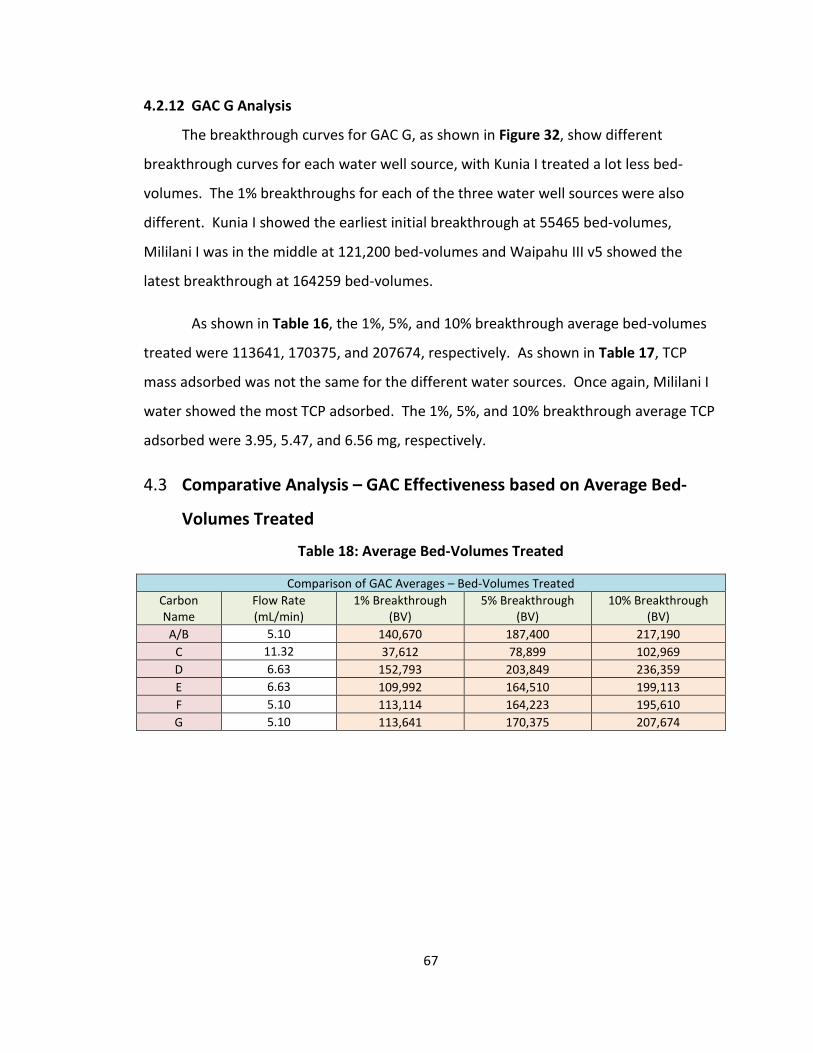
67
4.2.12 GAC G Analysis
The breakthrough curves for GAC G, as shown in Figure 32, show different
breakthrough curves for each water well source, with Kunia I treated a lot less bed-
volumes. The 1% breakthroughs for each of the three water well sources were also
different. Kunia I showed the earliest initial breakthrough at 55465 bed-volumes,
Mililani I was in the middle at 121,200 bed-volumes and Waipahu III v5 showed the
latest breakthrough at 164259 bed-volumes.
As shown in Table 16, the 1%, 5%, and 10% breakthrough average bed-volumes
treated were 113641, 170375, and 207674, respectively. As shown in Table 17, TCP
mass adsorbed was not the same for the different water sources. Once again, Mililani I
water showed the most TCP adsorbed. The 1%, 5%, and 10% breakthrough average TCP
adsorbed were 3.95, 5.47, and 6.56 mg, respectively.
Comparative Analysis – GAC Effectiveness based on Average Bed-4.3
Volumes Treated
Table 18: Average Bed-Volumes Treated
Comparison of GAC Averages – Bed-Volumes Treated Carbon Name
Flow Rate (mL/min)
1% Breakthrough (BV)
5% Breakthrough (BV)
10% Breakthrough (BV)
A/B 5.10 140,670 187,400 217,190 C 11.32 37,612 78,899 102,969 D 6.63 152,793 203,849 236,359 E 6.63 109,992 164,510 199,113 F 5.10 113,114 164,223 195,610 G 5.10 113,641 170,375 207,674

68
Table 19: Ranking GAC Effectiveness by GAC Type – Average Bed-Volumes Treated
Comparison of GAC Averages – Bed-Volumes Treated Ranking 1% Breakthrough 5% Breakthrough 10% Breakthrough Overall
#1 D D D D #2 A/B A/B A/B A/B #3 G G G G #4 F E E E #5 E F F F #6 C C C C
Table 20: Average TCP Mass Adsorbed per GAC Unit
Comparison of GAC Averages – TCP Mass Adsorbed per GAC Unit (mg) Carbon Name Flow Rate (mL/min) 1% Breakthrough 5% Breakthrough 10% Breakthrough
A/B 5.10 4.82 6.28 7.10 C 11.3 0.88 2.05 2.80 D 6.63 2.94 3.91 4.48 E 6.63 3.50 5.27 6.31 F 5.10 3.99 5.58 6.59 G 5.10 3.95 5.47 6.56
Table 21: Ranking Effectiveness by GAC Type – Average TCP Mass Adsorbed per GAC Unit
Comparison of GAC Averages – TCP Mass Adsorbed per GAC Unit (mg) Ranking 1% Breakthrough 5% Breakthrough 10% Breakthrough Overall
#1 A/B A/B A/B A/B #2 F F F F #3 G G G G #4 E E E E #5 D D D D #6 C C C C
The main objective of this study was to compare each of the six GACs to
determine which one was the most effective at TCP removal. The breakthrough of the
TCP contaminant was measured at 1%, 5%, and 10% breakthrough points. These
breakthrough points will give a good indication of the TCP breakthrough for each of the

69
GACs. The bed-volumes treated at the breakthrough points are used to evaluate the
effectiveness of the GACs. The more bed-volumes treated, the more effective the GAC.
The average bed-volumes treated for each GAC type and the ranking of the GAC
effectiveness based on these averages are shown Table 18 and Table 19. The averages
excluded outliers. It can be seen that GAC D had the highest average bed-volumes
treated for each of the breakthrough limits and GAC C had the lowest. These average
bed-volumes treated, however, are not a very accurate measurement because the bed-
volumes treated varies depending on the water well source. For a specific GAC, the
breakthrough curves for each of the three water well sources were not identical. This
means that there must be something different amongst the different water sources that
are affecting how the TCP is being adsorbed to the GAC. The water matrix of each water
well source must contain different concentrations of other contaminants. Also, because
there was no trend, like one water well source always treating more bed-volumes, the
different GAC types must not adsorb TCP in the same manner.
Therefore, it is not recommended to find a one-fits-all GAC to be applied for all
of Hawaii’s water treatment facilities, but rather to find a most effective GAC type
specific to the water well source. A GAC type that is the most effective for one
particular well could be the least effective for another well.

70
Results/Analysis by Water Well Source 4.4
4.4.1 Kunia I Results
Table 22: Kunia I Breakthrough Results – Bed-Volumes Treated
Kunia I – Bed-Volumes Treated Carbon Name
Flow Rate (mL/min) Version Run # 1%
Breakthrough 5%
Breakthrough 10%
Breakthrough A/B 5.10 v5 3 161,229 196,004 219,659
C 11.32 v5 2 51,230 97,142 113,325 D 6.63 v5 3 128,820 181,160 194,532 D 6.63 v5 8 164,224 214,707 245,779 E 6.63 v5 3 64,960 108,739 134,780 F 6.63 Wrong 3 56,787 106,151 137,539 F 5.10 v5 8 90,183 135,942 161,667 G 5.10 v5 8 130,546 100,264 150,391
Table 23: Kunia I – Effectiveness of GAC
Kunia I – Bed-Volumes Treated Ranking 1% Breakthrough 5% Breakthrough 10% Breakthrough Overall
#1 A/B D D D #2 D A/B A/B A/B #3 F F F F #4 E E G E #5 G G E G #6 C C C C
Table 24: Kunia I Breakthrough Results – TCP Mass Adsorbed per GAC Unit
Kunia I - TCP Mass Adsorbed per GAC Unit (mg) Carbon Name
Flow Rate (mL/min) Version Run # 1%
Breakthrough 5%
Breakthrough 10%
Breakthrough A/B 5.10 v5 3 3.48 4.20 4.67
C 11.32 v5 2 0.49 0.93 1.07
D 6.63 v5 3 2.78 3.87 4.13
D 6.63 v5 8 3.51 4.58 5.20
E 6.63 v5 3 1.40 2.32 2.84
F 6.63 Wrong 3 1.22 2.25 2.88
F 5.10 v5 8 1.96 2.93 3.45
G 5.10 v5 8 1.20 2.15 3.17

71
Figure 33: Kunia I Breakthrough Results
0
0.02
0.04
0.06
0.08
0.1
0 50000 100000 150000 200000 250000 300000 350000
TCP
Conc
netr
atio
n (p
pb)
Bed-volumes
TCP Breakthrough Curve - Kunia I
GAC A/B - v5
GAC C - v5
GAC D - v5 (run 3)
GAC D - v5 (run 8)
GAC E - v5
GAC F - wrong
GAC F - v5
GAC G - v5

72
4.4.2 Kunia I Analysis
The breakthrough curves for Kunia I water, as shown in Figure 33, are shown for
each GAC type. The bed-volumes treated, ranking of GAC effectiveness, and TCP
adsorbed of each GAC type at each breakthrough point are shown in Table 22, Table 23,
and Table 24, respectively. It is seen that GAC A/B and GAC D (both runs) showed the
most bed-volumes treated at all breakthrough points. It is seen that of all the GAC
types, GAC A/B treated the most bed-volumes at 1% breakthrough, while GAC D treated
the most at 5% and 10% breakthrough. The difference between the bed-volumes
treated between those two GACs was very close. GAC C treated the least bed-volumes
at each breakthrough point.
GAC C, E, F (wrong), and G all showed relatively close initial breakthrough values
at 50000 - 65000 bed-volumes. GAC E, F (wrong), and G showed very close patterns in
the breakthrough curve, while GAC C deviated to a steeper slope as the TCP
concentration increased. GAC F breakthrough curve was in between the low
breakthrough curve bunch and GAC A/B and D curve bunch. The data from the TCP
adsorbed was consistent with that of bed-volumes treated, as GAC A/B and D adsorbed
the most and GAC C adsorbed the least.
Based on the Kunia I results, GAC A/B and GAC D were the most effective and
GAC C was the least effective.

73
4.4.3 Waipahu III v3 Results
Table 25: Waipahu III v3 Breakthrough Results – Bed-Volumes Treated
Waipahu III v3 – Bed-Volumes Treated Carbon Name Flow Rate (mL/min) Version Run # 1% Breakthrough 5% Breakthrough 10% Breakthrough
A/B 4.35 v3 5 238,763 296,847 344,999 C 9.67 v3 5 65,147 109,268 128,116 D 5.66 v3 4 159,467 199,164 234,461 E 5.66 v3 4 66,507 101,033 186,156 F 4.35 v3 4 132,957 183,896 218,547 G 4.35 v3 5 174,595 219,551 258,980
Table 26: Waipahu III v3 – Effectiveness of GAC
Waipahu III v3 – Bed-Volumes Treated Ranking 1% Breakthrough 5% Breakthrough 10% Breakthrough Overall
#1 A/B A/B A/B A/B #2 G G G G #3 D D D D #4 F F F F #5 E C E E #6 C E C C
Table 27: Waipahu III v3 Breakthrough Results – TCP Mass Adsorbed per GAC Unit
Waipahu III v3 – TCP Mass Adsorbed per GAC Unit (mg) Carbon Name Flow Rate (mL/min) Version Run # 1% Breakthrough 5% Breakthrough 10% Breakthrough
A/B 4.35 v3 5 3.60 4.45 5.12 C 9.67 v3 5 0.98 1.63 1.89 D 5.66 v3 4 2.40 2.98 3.46 E 5.66 v3 4 1.00 1.50 2.69 F 4.35 v3 4 2.00 2.74 3.21 G 4.35 v3 5 2.63 3.28 3.83
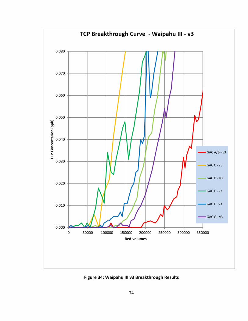
74
Figure 34: Waipahu III v3 Breakthrough Results
0.000
0.010
0.020
0.030
0.040
0.050
0.060
0.070
0.080
0 50000 100000 150000 200000 250000 300000 350000
TCP
Conc
enta
rion
(ppb
)
Bed-volumes
TCP Breakthrough Curve - Waipahu III - v3
GAC A/B - v3
GAC C - v3
GAC D - v3
GAC E - v3
GAC F - v3
GAC G - v3

75
4.4.4 Waipahu III v3 Analysis
The breakthrough curves for Waipahu III v5 water, as shown in Figure 34, are
shown for each GAC type. The bed-volumes treated, ranking of GAC effectiveness, and
TCP adsorbed of each GAC type at each breakthrough point are shown in Table 25,
Table 26, and Table 27, respectively. It can be seen that GAC A/B treated substantially
more bed-volumes and adsorbed more TCP at a given TCP concentration than any other
GACs and thus was the most effective GAC for Waipahu III v3. The next most treated
bed-volumes were GAC G, followed by GAC D, GAC F, GAC E, and GAC C. GAC C treated
the least bed-volumes at 1% and 10% breakthrough, while GAC E treated the least at 5%
breakthrough. Overall, GAC C was the least effective. GAC A/B’s 1%, 5%, and 10%
breakthrough bed-volumes treated were 238763, 296847, and 344999, respectively
which were substantially more than any other GAC type and water well sources
combination tested in the experiment. GAC G, GAC D, and GAC F showed similar
breakthrough values to each other as can be seen in Table 25. GAC C and E showed the
earliest initial breakthroughs at 65147 and 66507 bed-volumes respectively. GAC C
showed a smoother and steeper curve than GAC E. The jumps in concentrations in GAC
E were most likely due to human error. The different types of errors found in this study
are explained in section 4.7. The data from the TCP adsorbed was consistent with that
of bed-volumes treated, as GAC A/B adsorbed the most and GAC C adsorbed the least.
No conclusions were based off of Waipahu III v3 results.

76
4.4.5 Waipahu III v5 Results
Table 28: Waipahu III v5 Breakthrough Results – Bed-Volumes Treated
Waipahu III v5 – Bed-Volumes Treated Carbon Name Flow Rate (mL/min) Version Run # 1% Breakthrough 5% Breakthrough 10% Breakthrough
A/B 5.10 v5 9 102,778 160,689 201,499 C 11.32 v5 10 35,212 67,711 91,732 D 6.63 v5 9 159,063 209,765 252,562 E 6.63 v5 10 164,259 230,054 275,083 F 5.10 v5 9 122,887 184,938 218,307 G 5.10 v5 10 164,259 230,054 275,083
Table 29: Waipahu III v5 – Effectiveness of GAC
Waipahu III v5 – Bed-Volumes Treated Ranking 1% Breakthrough 5% Breakthrough 10% Breakthrough Overall
#1 E E E E #2 D D D D #3 F F F F #4 G G G G #5 A/B A/B A/B A/B #6 C C C C
Table 30: Waipahu III v5 Breakthrough Results – TCP Mass Adsorbed per GAC Unit
Waipahu III v5 – TCP Mass Adsorbed per GAC Unit (mg) Carbon Name Flow Rate (mL/min) Version Run # 1% Breakthrough 5% Breakthrough 10% Breakthrough
A/B 5.10 v5 9 1.77 2.74 3.39 C 11.32 v5 10 0.60 1.14 1.52 D 6.63 v5 9 2.74 3.59 4.30 E 6.63 v5 10 2.83 3.93 4.64 F 5.10 v5 9 2.11 3.16 3.68 G 5.10 v5 10 2.07 3.15 3.83

77
Figure 35: Waipahu III v5 Breakthrough Results
4.4.6 Waipahu III v5 Analysis
The breakthrough curves for Waipahu III v5 water, as shown in Figure 35, are
shown for each GAC type. The bed-volumes treated, ranking of GAC effectiveness, and
TCP adsorbed of each GAC type at each breakthrough point are shown in Table 28,
Table 29, and Table 30, respectively. It can be seen that GAC E treated the most bed-
volumes at each breakthrough point. This was followed by GAC D, then GAC F and GAC
G which showed nearly identical values, followed by GAC A/B, and GAC C. All the GACs
breakthrough curves were relatively close to each other except for GAC C. GAC C
treated the least bed-volumes at each breakthrough point. The data from the TCP
adsorbed was consistent with that of bed-volumes treated, as GAC E adsorbed the most
and GAC C adsorbed the least.
Based on Waipahu III v5 results, GAC E was the most effective and GAC C was the
least effective.
0.000
0.010
0.020
0.030
0.040
0.050
0.060
0.070
0.080
0 50000 100000 150000 200000 250000 300000 350000
TCP
Conc
entr
atio
n (p
pb)
Bed-volumes
TCP Breakthrough Curve - Waipahu III - v5
GAC A/B - v5
GAC C - v5
GAC D - v5
GAC E - v5
GAC F - v5
GAC G - v5

78
4.4.7 Mililani I Results
Table 31: Mililani I Breakthrough Results – Bed-Volumes Treated
Mililani I – Bed-Volumes Treated Carbon Name Flow Rate (mL/min) Version Run # 1% Breakthrough 5% Breakthrough 10% Breakthrough
A/B 5.10 v5 6 158,003 205,508 230,412 C 11.32 v5 6 26,395 71,843 103,852 D 6.63 v5 6 98,395 103,555 105,260 E 6.63 v5 7 100,757 154,738 187,475 F 5.10 v5 7 126,272 171,791 206,858 G 5.10 v5 7 121,200 170,807 197,542
Table 32: Mililani I – Effectiveness of GAC
Mililani I – Bed-Volumes Treated Ranking 1% Breakthrough 5% Breakthrough 10% Breakthrough Overall
#1 A/B A/B A/B A/B #2 F F F F #3 G G G G #4 E E E E #5 C C C C
Note: GAC D was omitted due to an experimental error
Table 33: Mililani I Breakthrough Results – TCP Mass Adsorbed per GAC Unit
Mililani I – TCP Mass Adsorbed per GAC Unit (mg) Carbon Name Flow Rate (mL/min) Version Run # 1% Breakthrough 5% Breakthrough 10% Breakthrough
A/B 5.10 v5 6 9.21 11.90 13.23 C 11.32 v5 6 1.53 4.09 5.80 D 6.63 v5 6 5.73 6.01 6.08 E 6.63 v5 7 6.29 9.56 11.44 F 5.10 v5 7 7.88 10.65 12.63 G 5.10 v5 7 7.80 10.34 11.88

79
Figure 36: Mililani I Breakthrough Results
4.4.8 Mililani I Analysis
The breakthrough curves for Mililani I water, as shown in Figure 36, are shown
for each GAC type. The bed-volumes treated, ranking of GAC effectiveness, and TCP
adsorbed of each GAC type at each breakthrough point are shown in Table 31, Table 32,
and Table 33, respectively. It can be seen that GAC A/B treated the most bed-volumes
at each breakthrough point compared to the other GACs. The GAC with the next most
treated bed-volumes was GAC F and G which showed nearly identical results, followed
by GAC E, GAC D, and GAC C. GAC C treated the least bed-volumes at each
breakthrough points. GAC C also had a 1% breakthrough of 26395 bed-volumes, the
lowest of any GAC and water well source combination. The other GACs showed 1%
breakthroughs ranging from 100757 to 158003 bed-volumes. GAC D’s results were
omitted due to the experimental error that was previously described. The data from the
TCP adsorbed was consistent with that of bed-volumes treated, as GAC A/B adsorbed
the most and GAC C adsorbed the least.
Based on Mililani I results, GAC A/B was the most effective and GAC C was the
least effective.
0.000
0.020
0.040
0.060
0.080
0.100
0.120
0.140
0.160
0.180
0.200
0.220
0 50000 100000 150000 200000 250000 300000 350000
TCP
Conc
entr
atio
n (p
pb)
Bed-volumes
TCP Breakthrough Curve - Mililani I
GAC A/B - v5
GAC C - v5
GAC D - v5
GAC E - v5
GAC F - v5
GAC G - v5

80
Comparative Analysis – GAC Effectiveness by Water Well Site 4.5
Table 34: GAC Effectiveness by Water Well Site
Overall Rank Kunia I Waipahu III Mililani I
#1 D E A/B
#2 A/B D F
#3 F G G
#4 E F E
#5 G A/B C
#6 C C
Table 35: Most and Least Effective GAC by Water Well SIte
Well Most Effective Least Effective Kunia I GAC D GAC A/B GAC C Waipahu III GAC E GAC C Mililani I GAC A/B GAC C
The effectiveness of the GAC type by each water well sources is shown in Table
34 and Table 35. It can be seen that the least effective GAC for each water well site was
GAC C. The most effective GAC was dependent on the water site. GAC D looked to be
effective for Kunia I and Waipahu III, but because of the error in Mililani I, it is unknown
how effective GAC D is for Mililani I. GAC A/B also was observed to be effective for
Kunia I and Mililani I, but it was not for Waipahu III.
For Kunia I, GAC A/B and D were the most effective and GAC C was the least. For
Waipahu III, GAC E was the most effective and GAC C was the least and for Mililani I,
GAC A/B was the most effective and GAC C was the least. In all three water well sources
tested, GAC C, the current GAC used, was the least effective GAC type.

81
Results/Analysis by GAC Particle Size 4.6
4.6.1 GAC Particle Size Results
Table 36: Properties of GAC Particle Size
Waipahu III GAC A/B U.S. Mesh Size Flow Rate
Largest ↑ ↓
Smallest
100 x 120 3.42 mL/min 120 x 140 4.07 mL/min 140 x 170 4.82 mL/min 170 x 200 5.74 mL/min
Bed Volume 0.355 mL TCP Influent 0.506 ppb
Table 37: GAC Particle Size Breakthrough Results – Bed-Volumes Treated
Waipahu III GAC A/B – Bed-Volumes Treated Carbon Size Flow Rate (mL/min) Run # 1% Breakthrough 5% Breakthrough 10% Breakthrough
Limiting Concentration (ppb) 0.0051 0.0253 0.0506 100 x 120 3.42 11 344,371 462,863 538,015 120 x 140 4.07 11 276,376 355,973 409,157 140 x 170 4.82 11 260,776 340,779 384,473 170 x 200 5.74 11 192,564 236,700 274,239
Table 38: GAC Particle Size – Effectiveness
Kunia I – Bed-Volumes Treated Ranking 1% Breakthrough 5% Breakthrough 10% Breakthrough Overall
#1 100 x 120 100 x 120 100 x 120 100 x 120 #2 120 x 140 120 x 140 120 x 140 120 x 140 #3 140 x 170 140 x 170 140 x 170 140 x 170 #4 170 x 200 170 x 200 170 x 200 170 x 200
Table 39: GAC Particle Size Breakthrough Results – TCP Mass Adsorbed per GAC Unit
Mililani I – TCP Mass Adsorbed per GAC Unit (mg) Carbon Name Flow Rate (mL/min) Run # 1% Breakthrough 5% Breakthrough 10% Breakthrough
Limiting Concentration (ppb) 0.0051 0.0253 0.0506 100 x 120 3.42 11 4.73 6.32 7.27 120 x 140 4.07 11 3.80 4.86 5.53 140 x 170 4.82 11 3.59 4.65 5.20 170 x 200 5.74 11 2.65 3.23 3.70

82
Figure 37: GAC Particle Size Breakthrough Results
4.6.2 Different GAC Particle Size Analysis
A comparative analysis was done to determine whether or not the GAC particle
size had an effect on the breakthrough curve. The GAC type and water site was held
constant. GAC A/B and Waipahu III water was selected for this study. Four different
GAC particle sizes were tested against each other. The tested GACs are from largest to
smallest GAC particles size; 100 x 120, 120 x 140, 140 x 170, and 170 x 200 mesh GACs.
The small-scale flow rate and column depth were scaled proportionally so that,
theoretically, the TCP breakthrough curves of each GAC particle size would be identical.
More on the column scaling calculation are in appendix 7.1
The breakthrough curves for the GAC particle size study, as shown in Figure 37,
are shown the different GAC particle sizes. The bed-volumes treated, ranking of GAC
0.000
0.010
0.020
0.030
0.040
0.050
0.060
0.070
0.080
0.090
0.100
0 100000 200000 300000 400000 500000 600000
TCP
Conc
entr
atio
n (p
pb)
Bedvolumes
Waipahu III - Carbon A/B (Run #11)
100 x 120 mesh
120 x 140 mesh
140 x 170 mesh
170 x 200 mesh

83
effectiveness, and TCP adsorbed of each GAC type at each breakthrough point are
shown in Table 37, Table 38, and Table 39, respectively. It can be seen that GAC 100 x
120 mesh size treated the most bed-volumes at each breakthrough point compared to
the other GACs. The GAC with the next most treated bed-volumes was GAC 120 x 140,
140 x 170, and 170 x 200 mesh size at each breakthrough point.
It is seen that the GAC particle size was related to the amount to reach its breakthrough
points. The larger the GAC particle size (smaller mesh #), the more bed-volumes it took
to reach its breakthrough limits. 170 x 200 mesh GAC broke through significantly earlier
than the others. 120 x 140 and 140 x 170 mesh GACs had nearly identical breakthrough
curves with a slight difference between the TCP concentrations of 0.020 - 0.030 ppb.
100 x 120 mesh GAC treated over 500000 bed-volumes before reaching a 10%
breakthrough.
Based on the results, the theoretical concept that the breakthrough curve would
be identical at different GAC particles sizes is not true. Even though the GAC was scaled
correctly, the size of the particles made a difference in the breakthrough curve. It was
seen that the smaller the GAC particle size, the less bed-volumes and less effective the
GAC was. This was contrary to what was believed. If the breakthrough curves were not
identical, it was thought that the smaller the GAC particle size, the more bed-volumes
and more effective the GAC was because there would be more surface area per GAC
pore volume. Since the results were like this, the accuracy of the RSSCT scaling
equations has been questioned.
Another interesting finding from this study was that GAC A/B performed a lot
better in this run than it did previously. Looking at the results, 170 x 200 mesh GAC A/B
Waipahu III treated 192564, 236700, and 274239 bed-volumes at 1%, 5%, and 10%
breakthrough while in the earlier run (run #9, p. 57), the same GAC treated 102778,
160689, and 201499 bed-volumes, respectively. If the latter run was the correct then
GAC A/B would be the most effective for Waipahu III as well. This adds evidence to
question the accuracy of the RSSCT scaling equations.

84
Error 4.7
Error has a significant impact on an experiment. There are many variations that
can occur due to error. This is a list of possible sources of error in our research:
1. Different people working on the same task of the experiment: This is a huge
source of error because different people will follow and perceive the same
experimental procedure differently. For example, the GAC grinding, sieving,
sampling, and TCP extractions were all done by multiple people. Small variations
in a protocol and operator technique can yield significantly different results.
2. The flow rate reading on the water pumping meters were not accurate to + 0.05
mL/min as previously mentioned. A manual calculation of dividing the treated
effluent water volume by the elapsed time was used to find the actual flow rate.
This flow rate was calculated between sampling times. Because of this, the flow
rates were not very accurate or consistent, especially for the first several flow
rates when the pumps were not calibrated to the right value.
3. The TCP extraction procedure used separatory funnels that are washed between
different samples. Failure to wash out the funnels thoroughly could easily result
in cross contamination.
4. The 2 mL of hexane that was measured during TCP extraction was measured by
the human eye. Just an incremental change in hexane added to the sample
could yield inaccurate results.
5. The 200 mL sample was measured in one graduated cylinder by the human eye.
Besides measurement errors, there is also a chance for cross contamination.
6. The water containers holding the tested water were not capped with a seal. This
was because the tube used to pump out the water interfered with capping. TCP
could have evaporated in the water containers due to imperfect sealing.
7. Only the initial set of influent water in a run was tested for TCP concentration.
This means if the influent TCP concentration varied at any given water well, the
results would be inaccurate.
85
8. The GAC columns (runs #2 - 10) were filled based on the amount to completely
fill the column volume. A more accurate method would be to weigh the GAC.
5 CONCLUSIONS A granular activated carbon (GAC) water treatment study was conducted to
evaluate six different types of GACs and determine their ability to absorb TCP, a
hazardous chemical compound found in Hawaii’s drinking water aquifers. The most
effective GAC type would be recommended as a replacement for the currently used GAC
unit in Hawaii’s water treatment facilities. A time efficient and economical method
called Rapid Small-Scale Column Test (RSSCT) was used to model a full-scale GAC unit
from a bench-scale test using small-scale columns.
The key findings from this study were:
• Any of the 6 GACs tested can meet the possible new 5 ppt MCL for TCP. This was
never known or tested for before in Hawaii. Analytical methods were able to
detect TCP concentration = 1 ppt. This was previously not thought to be
possible. This is a valuable finding. The State of Hawaii can lower its MCL to 5
ppt because all the tested GACs will be able to safely treat the TCP contaminated
groundwater. The duration the GAC can be used; however, it varies by GAC
type.
• GAC C, the GAC currently used in Hawaii’s water treatment facilities, was the
least effective GAC type in each of the three water well sources. It treated the
least bed-volumes by far. This is insightful because, based on the water wells
tested, any of the other GACs could replace the current one and be more
effective. Although other water wells could fair differently, it is highly unlikely
that GAC C would be the most effective GAC for any water source.
• There was no GAC that was the most effective for all three water sources;
therefore, it is not necessary to find a one-fits-all GAC to be applied for all of
Hawaii’s water treatment facilities, but rather a most effective GAC type specific

86
to the water well source. A GAC type that is the most effective for one particular
well could be the least effective for another well.
• The data suggests that the most effective GAC by water well source was:
o Kunia I – GAC A/B and D
o Waipahu III – GAC E
o Mililani I – GAC A/B
• The GAC particle size affects the effectiveness of GAC for TCP removal. The
smaller the GAC particle size, the less effective the GAC was. Even through the
GAC was proportionally scaled correctly, the particle size made a difference in
the breakthrough curve.
• The accuracy of the RSSCT scaling equations should be looked at in further
detail.
• Only TCP was analyzed in this study, however, other contaminants are in the
groundwater (natural organic matter, other volatile organic compounds,
pesticides, etc.) and they affect the GAC’s adsorption capacity for TCP.
• The GAC performance to effectively treat EDB and DBCP is important. It would
be taken into consideration when the selection of the most effective GAC to
treat Hawaii’s groundwater is made.
The findings from this RSSCT study are of great value and significance. Replacing
the currently used GAC unit with a more effective one means the units in the field would
need to be changed less frequently, thus saving on maintenance and operating costs.
6 REFERENCES . "1,2,3-trichloropropane (TCP)." Shef Leff Lawyers Protecting Water Retrieved 3 Oct, 2014, from http://www.sherleff.com/1-2-3-trichloropropane-tcp.html.
(2010). "Emerging Contaminant –1,2,3-Trichloropropane (TCP)." United States Environmental Protection Agency. (2011). Amendment and Compilation of Chapter 11-20 Hawaii Administrative Rules. D. o. Health: p. 20-14.

87
(2014). "1,2,3,-Trichloropropane." California Environmental Protection Agency State Water Resources Control Board Retrieved 2014, 4 Oct, from http://www.waterboards.ca.gov/drinking_water/certlic/drinkingwater/123TCP.shtml. (Cal/EPA), C. E. P. A. (2009). Groundwater Information Sheet 1,2,3 - Trichloropropane (TCP). Groundwater Ambient Monitoring and Assessment (GAMA) Program. S. W. R. C. Board. (CDPH), C. D. o. P. H. (2002a). Determination of 1,2,3-Trichloropropane in Drinking Water by Continuous Liquid-Liquid Extraction and Gas Chromatography/Mass Spectrometry.
(DHHS), U. S. D. o. H. a. H. S. (2011). "Report on Carcinogens, 12th Edition." Public Health Service, National Toxicology Program 12th Edition.
(HSDB), H. S. D. B. (2009). "1,2,3-Trichloropropane." (IRIS), E. I. R. I. S. (2009). 1,2,3-Trichloropropane (CASRN 96-18-4). (NIOSH), N. I. f. O. S. a. H. (2010). "1,2,3 - Trichloropropane." NIOSH Pocket Guide to Chemical Hazards. (OEHHA), C. O. o. E. H. H. A. (2009). "Announcement of Publication of the First Public Health Goal for 1,2,3 - Trichloropropane in Drinking Water." Administration, O. S. H. (2013). 1,2,3-Trichloropropane. AECOM (2014). Board of Water Supply TCP Removal Work Plan Item 5 A – Rapid Small Scale Column Testing. Agency, E. U. S. E. P. (2013). Technical Fact Sheet –1,2,3-Trichloropropane (TCP). O. o. S. W. a. E. R. (5106P): p. 1-5. ATSDR. (1992). "Toxicological Profile for 1,2,3-Trichloropropane." Retrieved 3 Oct, 2014, from http://www.atsdr.cdc.gov/toxprofiles/tp57.pdf. ATSDR (1995). 1,2,3-Trichloropropane. U.S. Department of Health and Human Services. A. A. f. T. S. a. D. R. ToxFAQs. Berrigan, J. K. (1985). "Scale - Up of Rapid Small - Scale Adsorption Test to Field -- Scale Adsorber: Theoretical and Experimental Basis." Nat. Tech. Info. Svc. Berrigan, J. K. (1985). Scale - Up of Rapid Small - Scale Adsorption Tests to Field - Scale Adsorbers: Theoretical and Experimental Basis. M.S., Michigan Technological University, Houghton. CDPH (2002b). "Determination of 1,2,3-Trichloropropane in Drinking Water by Purge and Trap Gas Chromatography/Mass Spectrometry."

88
Corporation, C. (1992). Granular Activated Carbon for Water & Wastewater Treatment. Corwin, C. J. and R. S. Summers (2010). "Scaling Trace Organic Contaminant Adsorption Capacity by Granular Activated Carbon." Environmental Science & Technology 44(14): 5403-5408. Crittenden, J. C., J. K. Berrigan and D. W. Hand (1986). "Design of Rapid Small-Scale Adsorption Tests for a Constant Diffusivity." Journal Water Pollution Control Federation 58(4): 312-319. Crittenden, J. C., J. K. Berrigan, D. W. Hand and B. Lykins (1987). "Design of Rapid Fixed-Bed Adsorption Tests for Nonconstant Diffusivities." Journal of Environmental Engineering-Asce 113(2): 243-259. Crittenden, J. C., P. S. Reddy, H. Arora, J. Trynoski, D. W. Hand, D. L. Perram and R. S. Summers (1991). "Predicting Gac Performance with Rapid Small-Scale Column Tests." Journal American Water Works Association 83(1): 77-87. Dobrzelewski, M. (1985). "Determination and Prediction of Surface Diffusivities of Volatile Organic Copounds Found in Drinking Water." Nat. Tech. Info Svc. E. J. Wilson, a. C. J. G. (1966). "Liquid Mass Transfer at Very Low Reynolds Number in Packed Beds." Ind. Eng. Chem. Fundam. EPA (1990). Method 551.1. “Determination of Chlorination Disinfection Byproducts, Chlorinated Solvents, and Halogenated Pesticides/Herbicides in Drinking Water by Liquid-Liquid Extraction and Gas Chromatography with Electron-Capture Detection.". O. o. R. a. D. (ORD). EPA (1995). Method 504.1 “1,2-Dibromoethane (EDB), 1,2-Dibromo-3-chloropropane (DBCP), and 1,2,3-Trichloropropane (123TCP) in Water by Microextraction and Gas Chromatography. O. o. R. a. D. (ORD). EPA (1996). "Method 8260B "Volatile Organic Compounds by Gas Chromatography/Mass Spectrometry (GC/MS)"." (Revision 2). EPA (2009). Method 524.3. “Measurement of Purgeable Organic Compounds in Water by Capillary Column Gas Chromatography/Mass Spectrometry.”. O. o. G. a. D. W. (OGWDW).
EPA (2012a). 2012 Edition of the Drinking Water Standards and Health Advisories. EPA (2013). "Regional Screening Levels (RSL) Summary Table." EPA (2014). Granular Activated Carbon. Eric P. Hooker, M., DABT, M. Keri G. Fulcher, P. Herman J. Gibb, MPH, T. T. Sciences and V. Arlington (2012). Report to the Hawaii Department of Health, Safe Drinking Water Branch,Regarding the Human Health Risks of 1,2,3-Trichloropropane in Tap Water, Tetra Tech: p. 1-97.

89
F. Bianchi, M. Careri, A. Mangia and M. Musci (2007). "Retention indices in the analysis of food aroma volatile compounds in temperature-programmed gas chromatography: database creation and evaluation of precision and robustness." J. Sep. Sci.(30): p. 563 - 572. Fotta, M. E. (2012). Effect of Granular Activated Carbon Type on Adsorber Performance and Scale-Up Approaches for Volatile Organic Compound Removal. Master of Science, North Carolina State University. Glaze, W. W. and C. C. Lin (1984). "Optimization of Liquid-Liquid Extraction Methods for Analysis of Organics in Water." ( January 1984). Glenn Dombeck, P. E. and C. Borg Multi-contaminant Treatment for 1,2,3 Trichloropropane Destruction Using the HiPOx Reactor. Henderson, J. E., G. R. Peyton and W. H. Glaze (1976). "In Identification and Analysis of Organic Pollutants in Water (L.H. Keith ed.)." pp. 105-111. HSDB ( 1989). Hazardous Substance Data Bank. National Library of Medicine,National Toxicology Information Program. Jenoptik. "Adsorptive exhaust treatment; kinetics and mass transfer zone." Retrieved Nov. 19, 2014, from http://www.jenoptik.com/Internet_EN_Adsorptive_Abluftreinigung_Kinetik_und_Massentransferzone. Jenoptik. "Properties of adsorbents." Retrieved Nov. 19, 2014, from http://www.jenoptik.com/Internet_EN_Eigenschaften_der_Adsorbentien. Khan, E., Wirojanaqud, W., and N. Sermsai (2009). Effects of Iron Type in Fenton Reaction on Mineralization and Biodegradability Enhancement of Hazardous Organic Compounds. Volume 161 Pages 1024 to 1034. Knappe, D., V. Snoeyink, P. Roche, M. Prados, and and M. Bourbigot (1997). The Effect of Preloading on RSSCT Predictions of Atrazine Removal By GAC Adsorbers. Water Research. Vol. 31: p. 2899 - 2909. Lamichhane, K. (2014). Sorption, UH - Manoa. Lenntech. (2014). "Adsorption / Active Carbon." Retrieved 9 Oct, 2014, from http://www.lenntech.com/library/adsorption/adsorption.htm. Materials, A. S. f. T. a. (2008). Standard Practice for the Prediction of Contaminant Adsorption on GAC in Aqueous Systems Using Rapid Small-Scale Column Tests. D-6586-03.

90
Matsui S, M. T., Sasaki T and e. al (1975). Activated sludge degradabilityof organic substances in the waste water of the Kashima petroleum andpetrochemical industrial complex in Japan, Prog Water Technol Molnaa, B. ( 2003). “1,2,3-TCP: California’s Newest Emerging Contaminant, ENTECH Noonan, D. C. and J. T. Curtis (1990). Groundwater Remediation and Petroleum: A Guide for Underground Storage Tanks. Chelsea, MI, Lewis Pulishers. Oki, D. S. and T. W. Giambelluca (1987). "DCBP, EDB, and TCP Contamination of Ground Water in Hawaii." GROUND WATER Vol. 25(Nov-Dec 1987): p. 693-702.
Owen, D. M., Z. K. Chowdbury, R. S. Summers, S. M. Hooper, and and G. Solarik (1996). "Determination of Technology and Costs for GAC Treatment Using ICR Methodology" AWWA GAC & Membrane Workshop(March 1996).
Richard, J. J. and G. A. Junk (1977). "Liquid Extraction for Rapid Determination of Halomethanes in Water." Journal AWWA(January 1977). Samin, G. and D. B. Janssen (2012). "Transformation and biodegradation of 1,2,3-trichloropropane (TCP)." Environmental Science and Pollution Research International. Stepek, J. (2009). 1,2,3Trichloropropane (TCP), State Water Resources Control Board Division of Water Quality GAMA Program Summers, R. S., S. M. Hooper, G. Solarik, D. M. Owen and S. H. Hong (1995). "Bench-Scale Evaluation of Gac for Nom Control." Journal American Water Works Association 87(8): 69-80.
Tratnyek, P. G., V. Sarathy and J. H. Fortuna (2008). "“Fate and Remediation of 1,2,3-
Trichloropropane.” Remediation of Chlorinated and Recalcitrant Compounds-2008." Proceedings of the Sixth International Conference on Remediation of Chlorinated and Recalcitrant Compounds.
Veatch, B. (2008). Evaluation & Assessment of Removal Technology for Specific Organic Contaminants in NJ Drinking Water. Weber, J. B. (1993). Properties and behaivor of pesticides in soil, Lewis Publishers Westerhoff, P. (2004). "Rapid Small Scale Column Test (RSSCT) - Procedures for Arsenic Studies and Apllications of Results." Retrieved 3 Oct, 2014, from http://epa.gov/nrmrl/wswrd/dw/arsenic/pubs/rssctAsteststudy.pdf.
Williamson, J. E. (1963). "Liquid - Phase Mass Transfer at Low Reynolds Numbers." Ind. Eng. Chem. Fundam.

92
7 APPENDIX Column Sizing Calculations 7.1
7.1.1 Full-Scale Column Parameters (Given)
GAC Weight/Adsorber, WLC 30,000 lb GAC Specific Gravity, SGLC 0.500 Flow Rate, QLC 1 MGD Column Diameter, CDLC 12 ft Water Specific Weight, γW @ 20° C 62.3 lb/ft3
𝐶𝑔𝑔𝑔𝑔 𝑆𝑅𝑆𝑡𝑤𝑔𝐶𝑎𝑆 𝐴𝑔𝑅𝑎,𝐴𝐿𝐿 =𝜋4𝐶𝐶𝐿𝐿2 =
𝜋4∗ (3.6576 m)2 = 𝟏𝟏.𝟓𝟏 𝒎𝟐
𝐶𝑔𝑆𝐶𝑚𝐶 𝑉𝑔𝑆𝐶𝑚𝑅,𝑉𝑔𝑆𝐿𝐿 = 𝑊𝐿𝐿
𝛾𝑊 × 𝑆𝑆𝐿𝐿 =
30,000 𝑆𝑎
�62.3 𝑆𝑎𝑓𝑡3� (0.5)
= 𝟐𝟐.𝟐𝟓 𝒎𝟑
𝐶𝑔𝑆𝐶𝑚𝐶 𝐶𝑅𝑝𝑡ℎ, 𝐿𝐿𝐿 = 𝑉𝑔𝑆𝐿𝐿𝐴𝐿𝐿
=27.25 𝑚3
10.51 𝑚2 = 𝟐.𝟓𝟓 𝒎
𝑉𝑅𝑆𝑔𝑆𝑤𝑡𝑉,𝑉𝐿𝐿 =𝑄𝐿𝐿𝐴𝐿𝐿
=�1 ∗ 106𝑔𝑎𝑆
𝑑𝑎𝑉 � � 1 𝑓𝑡37.48 𝑔𝑎𝑆� �
13𝑚3
3.283 𝑓𝑡3� �1 𝑑𝑎𝑉24 ℎ𝑔�
10.51 𝑚2 = 𝟏𝟓.𝟏𝒎𝒉𝒉
𝐸𝐸𝐶𝐸𝐿𝐿 =𝑉𝑔𝑆𝐿𝐿𝑄𝐿𝐿
=27.25 𝑚3
�1 ∗ 106𝑔𝑎𝑆𝑑𝑎𝑉 � � 1 𝑓𝑡3
7.48 𝑔𝑎𝑆� �13𝑚3
3.283 𝑓𝑡3� �1 𝑑𝑎𝑉
1440 𝑚𝑤𝐶�= 𝟏𝟏.𝟑𝟑 𝒎𝒎𝒎
𝐸𝑅𝑑 − 𝑉𝑔𝑆𝐶𝑚𝑅𝑔 𝐸𝑔𝑅𝑎𝑡𝑅𝑑 𝑝𝑅𝑔 𝐶𝑎𝑉 =1 𝑑𝑎𝑉𝐸𝐸𝐶𝐸𝐿𝐿
=1 𝑑𝑎𝑉
(10.36 𝑚𝑤𝐶) � 1 𝑑𝑎𝑉1440 𝑚𝑤𝐶�
= 𝟏𝟑𝟓.𝟏 𝑩𝑩𝒅𝒅𝒅

93
𝐸𝑤𝑚𝑅 𝑡𝑔 𝑅𝑅𝑎𝑆ℎ 100,000 𝐸𝑉 =100,000 𝐸𝑉
�139.0 𝐸𝑉𝑑𝑎𝑉�= 𝟏𝟏𝟑.𝟖 𝒅𝒅𝒅𝒅
𝑉𝑔𝑆𝐶𝑚𝑅 𝑡𝑔 𝐸𝑔𝑅𝑎𝑡 100,000 𝐸𝑉 = (𝐸𝑤𝑚𝑅 𝑡𝑔 𝑅𝑅𝑎𝑆ℎ 100,000 𝐸𝑉)(𝑄𝐿𝐿) = (143.8 𝑑𝑎𝑉𝑔) �1 ∗ 106𝑔𝑎𝑆
𝑑𝑎𝑉� �
1 𝑓𝑡3
7.48 𝑔𝑎𝑆��
13𝑚3
3.283 𝑓𝑡3� �
1000 𝐿1 𝑚3 � = 𝟓.𝟏𝟓 × 𝟏𝟏𝟖 𝑳
7.1.2 Full – Scale GAC Particle Sizes
GAC ID U.S. Mesh Size No Corresponding Particle Size Calculation of Average Particle Size Average Particle Size Passed Retained Passed Retained
GAC A/B 12 40 1.68 mm 0.42 mm 1.68 𝑚𝑚 + 0.42 𝑚𝑚
2 1.00 mm
GAC C 8 30 2.38 mm 0.595 mm 2.38 𝑚𝑚 + 0.595 𝑚𝑚2
1.49 mm
GAC D 12 30 1.68 mm 0.595 mm 1.68 𝑚𝑚 + 0.595 𝑚𝑚
2 1.14 mm
GAC E 12 30 1.68 mm 0.595 mm 1.68 𝑚𝑚 + 0.595 𝑚𝑚2
1.14 mm
GAC F 12 40 1.68 mm 0.42 mm 1.68 𝑚𝑚 + 0.42 𝑚𝑚
2 1.00 mm
GAC G 12 40 1.68 mm 0.42 mm 1.68 𝑚𝑚 + 0.42 𝑚𝑚
2 1.00 mm
Note: The average particle sizes of 1.00 mm should be 1.05 mm, but there was a calculation error. 1.00 mm was used in the calculations for runs #2 – 10 since the error was only caught after the test was completed.

94
7.1.3 Full – Scale Reynold’s Number Parameters
Velocity, VLC 15.0 m/hr Avg. Diameter, DLC (GAC A/B, F, and G) 1.00 mm Avg. Diameter, DLC (GAC D, and E) 1.14 mm Avg. Diameter, DLC (GAC C) 1.49 mm Kinematic Viscosity, νw @ 20° C 1.004 X 10⁻⁶ m2/s ReLC,min (Sieve No. 170 x 200) 0.39
7.1.4 Given Small-Scale (RSSCT) Column Parameters
Column Diameter, CDSC 4.76 mm GAC Specific Gravity, SGSC 0.500 Water Density, ρW 0.998 g/mL Column Depth, LSC (run #2 – 10) 2.00 cm
𝐶𝑔𝑔𝑔𝑔 𝑆𝑅𝑆𝑡𝑤𝑔𝐶𝑎𝑆 𝐴𝑔𝑅𝑎,𝐴𝑆𝐿 =𝜋4𝐶𝐶𝑆𝐿2 =
𝜋4∗ (4.76 𝑚𝑚)2 �
12 𝑆𝑚2
102 𝑚𝑚2� = 𝟏.𝟏𝟐𝟖 𝒄𝒎𝟐
𝐶𝑔𝑆𝐶𝑚𝐶 𝑉𝑔𝑆𝐶𝑚𝑅,𝑉𝑔𝑆𝑆𝐿 = 𝐴𝑆𝐿 ∗ 𝐿𝑆𝐿 = (0.178 𝑆𝑚2)(2.00 𝑆𝑚) �1 𝑚𝐿1 𝑆𝑚3� = 𝟏.𝟑𝟓𝟓 𝒎𝑳 ← (𝐫𝐫𝐫 #𝟐 – 𝟏𝟏)
𝑆𝐴𝐶 𝑀𝑎𝑔𝑔 = 𝑚𝑆𝐿 = 𝜌𝑆𝐿 ∗ 𝑉𝑔𝑆𝑆 = 𝑆𝑆𝑆𝐿 ∗ 𝜌𝑊 ∗ 𝑉𝑔𝑆𝑆 = (0.5) ∗ �0.998𝑔𝑚𝐿
� ∗ 0.355 𝑚𝐿 = 𝟏.𝟏𝟐𝟖 𝒈

95
7.1.5 Small-Scale (RSSCT) GAC Particle Sizes
Run # U.S. Mesh Size No Corresponding Particle Size Calculation of Average Particle Size Average Particle Size Passed Retained Passed Retained
2 – 10 170 200 0.088 mm 0.075 mm 0.088 𝑚𝑚 + 0.075 𝑚𝑚2
0.082 mm
11 170 200 0.088 mm 0.075 mm 0.088 𝑚𝑚 + 0.075 𝑚𝑚2
0.082 mm
11 140 170 0.106 mm 0.088 mm 0.106 𝑚𝑚 + 0.088 𝑚𝑚
2 0.097 mm
11 120 140 0.124 mm 0.106 mm 0.124 𝑚𝑚 + 0.106 𝑚𝑚
2 0.115 mm
11 100 120 0.149 mm 0.124 mm 0.149 𝑚𝑚 + 0.124 𝑚𝑚
2 0.137 mm
7.1.6 Calculation for Small – Scale Parameters
Runs #2 – 10: Comparative Evaluation of Different GACs
GAC A/B, GAC F, and GAC G
Full – Scale, DLC Small – Scale, DSC
1.00 mm 0.082 mm
𝐸𝐸𝐶𝐸𝑆𝐿𝐸𝐸𝐶𝐸𝐿𝐿
= �𝑅𝑆𝐿𝑅𝐿𝐿
�2
= ��𝐶𝑆𝐿2 �
�𝐶𝐿𝐿2 ��
2
= �𝐶𝑆𝐿𝐶𝐿𝐿
�2
𝐸𝐸𝐶𝐸𝑆𝐿 = 𝐸𝐸𝐶𝐸𝐿 ∗ �𝐶𝑆𝐿𝐶𝐿𝐿
�2
= (10.355 min) ∗ �0.082 𝑚𝑚1.00 𝑚𝑚
�2
= 0.070 𝑚𝑤𝐶

96
𝑉𝑅𝑆𝑔𝑆𝑤𝑡𝑉, 𝑉𝑆𝐿 =𝐿𝑆𝐿
𝐸𝐸𝐶𝐸𝑆𝐿=
(2.00 𝑆𝑚) � 1 𝑚100 𝑆𝑚�
(0.070 min) � 60 𝑔1 𝑚𝑤𝐶�
= 4.76 ∗ 10−3𝑚𝑔
𝑅𝑅𝑉𝐶𝑔𝑆𝑑′𝑔 𝑁𝐶𝑚𝑎𝑅𝑔,𝑅𝑅𝑚𝑖𝑛 = 𝑉𝑆𝐿 ∗ 𝐶𝑆𝐿
ν𝑊=�4.76 ∗ 10−3 𝑚𝑔 � (0.082 𝑚𝑚) � 1 𝑚
1000 𝑚𝑚�
�1.004 ∗ 10−6 𝑚2
𝑔 �= 0.39
𝐹𝑆𝑔𝑤 𝑅𝑎𝑡𝑅,𝑄𝑆𝐿 =𝑉𝑔𝑆𝑆𝐿𝐸𝐸𝐶𝐸𝑆𝐿
=0.355 𝑚𝐿0.070 𝑚𝑤𝐶
= 5.10 𝑚𝐿𝑚𝑤𝐶
𝐸𝑅𝑑 − 𝑉𝑔𝑆𝐶𝑚𝑅𝑔 𝐸𝑔𝑅𝑎𝑡𝑅𝑑 𝑝𝑅𝑔 𝐶𝑎𝑉 =1 𝑑𝑎𝑉𝐸𝐸𝐶𝐸𝑆𝐿
=1 𝑑𝑎𝑉
(0.070 𝑚𝑤𝐶) � 1 𝑑𝑎𝑉1440 𝑚𝑤𝐶�
= 𝟐𝟏,𝟑𝟐𝟖 𝑩𝑩𝒅𝒅𝒅
𝐸𝑤𝑚𝑅 𝑡𝑔 𝑅𝑅𝑎𝑆ℎ 100,000 𝐸𝑉 =100,000 𝐸𝑉
�20,678 𝐸𝑉𝑑𝑎𝑉�= 𝟏.𝟖𝟏 𝒅𝒅𝒅𝒅
𝑉𝑔𝑆𝐶𝑚𝑅 𝑡𝑔 𝐸𝑔𝑅𝑎𝑡 100,000 𝐸𝑉 = (𝐸𝑤𝑚𝑅 𝑡𝑔 𝑅𝑅𝑎𝑆ℎ 100,000 𝐸𝑉)(𝑄𝑆𝐿) = (4.84 𝑑𝑎𝑉𝑔) �5.10 𝑚𝐿𝑚𝑤𝐶
� �1440 𝑚𝑤𝐶
1 𝑑𝑎𝑉� �
1 𝐿1000 𝑚𝐿
� = 𝟑𝟓.𝟓 𝑳

97
GAC D and GAC E
Full – Scale, DLC Small – Scale, DSC
1.14 mm 0.082 mm
𝐸𝐸𝐶𝐸𝑆𝐿 = 𝐸𝐸𝐶𝐸𝐿 ∗ �𝐶𝑆𝐿𝐶𝐿𝐿
�2
= (10.355 min) ∗ �0.082 𝑚𝑚1.14 𝑚𝑚
�2
= 0.054 𝑚𝑤𝐶
𝐹𝑆𝑔𝑤 𝑅𝑎𝑡𝑅,𝑄𝑆𝐿 =𝑉𝑔𝑆𝑆𝐿𝐸𝐸𝐶𝐸𝑆𝐿
=0.355 𝑚𝐿0.054 𝑚𝑤𝐶
= 6.63 𝑚𝐿𝑚𝑤𝐶
𝐸𝑅𝑑 − 𝑉𝑔𝑆𝐶𝑚𝑅𝑔 𝐸𝑔𝑅𝑎𝑡𝑅𝑑 𝑝𝑅𝑔 𝐶𝑎𝑉 =1 𝑑𝑎𝑉𝐸𝐸𝐶𝐸𝑆𝐿
=1 𝑑𝑎𝑉
(0.054 𝑚𝑤𝐶) � 1 𝑑𝑎𝑉1440 𝑚𝑤𝐶�
= 𝟐𝟑,𝟖𝟐𝟑 𝑩𝑩𝒅𝒅𝒅
𝐸𝑤𝑚𝑅 𝑡𝑔 𝑅𝑅𝑎𝑆ℎ 100,000 𝐸𝑉 =100,000 𝐸𝑉
�26,873 𝐸𝑉𝑑𝑎𝑉�= 𝟑.𝟐𝟐 𝒅𝒅𝒅𝒅
𝑉𝑔𝑆𝐶𝑚𝑅 𝑡𝑔 𝐸𝑔𝑅𝑎𝑡 100,000 𝐸𝑉 = (𝐸𝑤𝑚𝑅 𝑡𝑔 𝑅𝑅𝑎𝑆ℎ 100,000 𝐸𝑉)(𝑄𝑆𝐿) = (3.72 𝑑𝑎𝑉𝑔) �6.63 𝑚𝐿𝑚𝑤𝐶
� �1440 𝑚𝑤𝐶
1 𝑑𝑎𝑉� �
1 𝐿1000 𝑚𝐿
� = 𝟑𝟓.𝟓 𝑳

98
GAC C
Full – Scale, DLC Small – Scale, DSC
1.49 mm 0.082 mm
𝐸𝐸𝐶𝐸𝑆𝐿 = 𝐸𝐸𝐶𝐸𝐿 ∗ �𝐶𝑆𝐿𝐶𝐿𝐿
�2
= (10.355 min) ∗ �0.082 𝑚𝑚1.49 𝑚𝑚
�2
= 0.031 𝑚𝑤𝐶
𝐹𝑆𝑔𝑤 𝑅𝑎𝑡𝑅,𝑄𝑆𝐿 =𝑉𝑔𝑆𝑆𝐿𝐸𝐸𝐶𝐸𝑆𝐿
=0.355 𝑚𝐿0.031 𝑚𝑤𝐶
= 11.32 𝑚𝐿𝑚𝑤𝐶
𝐸𝑅𝑑 − 𝑉𝑔𝑆𝐶𝑚𝑅𝑔 𝐸𝑔𝑅𝑎𝑡𝑅𝑑 𝑝𝑅𝑔 𝐶𝑎𝑉 =1 𝑑𝑎𝑉𝐸𝐸𝐶𝐸𝑆𝐿
=1 𝑑𝑎𝑉
(0.031 𝑚𝑤𝐶) � 1 𝑑𝑎𝑉1440 𝑚𝑤𝐶�
= 𝟏𝟓,𝟓𝟏𝟐 𝑩𝑩𝒅𝒅𝒅
𝐸𝑤𝑚𝑅 𝑡𝑔 𝑅𝑅𝑎𝑆ℎ 100,000 𝐸𝑉 =100,000 𝐸𝑉
�45,907 𝐸𝑉𝑑𝑎𝑉�= 𝟐.𝟏𝟖 𝒅𝒅𝒅𝒅
𝑉𝑔𝑆𝐶𝑚𝑅 𝑡𝑔 𝐸𝑔𝑅𝑎𝑡 100,000 𝐸𝑉 = (𝐸𝑤𝑚𝑅 𝑡𝑔 𝑅𝑅𝑎𝑆ℎ 100,000 𝐸𝑉)(𝑄𝑆𝐿) = (2.18 𝑑𝑎𝑉𝑔) �11.32 𝑚𝐿𝑚𝑤𝐶
� �1440 𝑚𝑤𝐶
1 𝑑𝑎𝑉� �
1 𝐿1000 𝑚𝐿
� = 𝟑𝟓.𝟓 𝑳

99
Run #11 Calculations: Comparative Evaluation of Carbon A/B for Different Small – Scale GAC Particle Sizes\
GAC A/B – Small – Scale 100 x 120 Mesh
Full – Scale, DLC Small – Scale, DSC
1.05 mm 0.137 mm
𝐸𝐸𝐶𝐸𝑆𝐿 = 𝐸𝐸𝐶𝐸𝐿𝐿 ∗ �𝐶𝑆𝐿𝐶𝐿𝐿
�2
= (10.355 min) ∗ �0.137 𝑚𝑚1.05 𝑚𝑚
�2
= 0.176 𝑚𝑤𝐶
𝑉𝑅𝑆𝑔𝑆𝑤𝑡𝑉,𝑉𝑆𝐿 = 𝑅𝑅𝑚𝑖𝑛 ∗ 𝜈𝑊
𝐶𝑆𝐿=
(0.436) �1.004 ∗ 10−6 𝑚2
𝑔 ��3600 𝑔
1 ℎ𝑔 �
(0.137 𝑚𝑚) � 1 𝑚1000 𝑚𝑚�
= 11.47𝑚ℎ𝑔
𝐶𝑔𝑆𝐶𝑚𝐶 𝐶𝑅𝑝𝑡ℎ, 𝐿𝑆𝐿 = 𝑉𝑆𝐿 ∗ 𝐸𝐸𝐶𝐸𝑆𝐿 = �11.47𝑚ℎ𝑔� (0.176 min) �
1 ℎ𝑔60 𝑚𝑤𝐶
� �100 𝑆𝑚
1 𝑚� = 3.37 𝑆𝑚
𝐶𝑔𝑆𝐶𝑚𝐶 𝑉𝑔𝑆𝐶𝑚𝑅,𝑉𝑔𝑆𝑆𝐿 = 𝐴𝑆𝐿 ∗ 𝐿𝑆𝐿 = (0.178 𝑆𝑚2)(3.37 𝑆𝑚) �1 𝑚𝐿1 𝑆𝑚3� = 0.599 𝑚𝐿
𝐹𝑆𝑔𝑤 𝑅𝑎𝑡𝑅,𝑄𝑆𝐿 =𝑉𝑔𝑆𝑆𝐿𝐸𝐸𝐶𝐸𝑆𝐿
=0.599 𝑚𝐿0.176 𝑚𝑤𝐶
= 3.42 𝑚𝐿𝑚𝑤𝐶
𝑆𝐴𝐶 𝑀𝑎𝑔𝑔 = 𝑚𝑆𝐿 = 𝜌𝑆𝐿 ∗ 𝑉𝑔𝑆𝑆 = 𝑆𝑆𝑆𝐿 ∗ 𝜌𝑊 ∗ 𝑉𝑔𝑆𝑆 = (0.5) ∗ �0.998𝑔𝑚𝐿
� ∗ 0.599 𝑚𝐿 = 𝟏.𝟐𝟓𝟓 𝒈
𝐸𝑅𝑑 − 𝑉𝑔𝑆𝐶𝑚𝑅𝑔 𝐸𝑔𝑅𝑎𝑡𝑅𝑑 𝑝𝑅𝑔 𝐶𝑎𝑉 =1 𝑑𝑎𝑉𝐸𝐸𝐶𝐸𝑆𝐿
=1 𝑑𝑎𝑉
(0.176 𝑚𝑤𝐶) � 1 𝑑𝑎𝑉1440 𝑚𝑤𝐶�
= 𝟖,𝟏𝟑𝟐 𝑩𝑩𝒅𝒅𝒅
𝐸𝑤𝑚𝑅 𝑡𝑔 𝑅𝑅𝑎𝑆ℎ 100,000 𝐸𝑉 =100,000 𝐸𝑉
�8,167 𝐸𝑉𝑑𝑎𝑉�
= 𝟏𝟐.𝟐𝟏 𝒅𝒅𝒅𝒅
𝑉𝑔𝑆𝐶𝑚𝑅 𝑡𝑔 𝐸𝑔𝑅𝑎𝑡 100,000 𝐸𝑉 = (𝐸𝑤𝑚𝑅 𝑡𝑔 𝑅𝑅𝑎𝑆ℎ 100,000 𝐸𝑉)(𝑄𝑆𝐿) = (12.24 𝑑𝑎𝑉𝑔) �3.42 𝑚𝐿𝑚𝑤𝐶
� �1440 𝑚𝑤𝐶
1 𝑑𝑎𝑉� �
1 𝐿1000 𝑚𝐿
� = 𝟑𝟏.𝟑 𝑳

100
GAC A/B – Small – Scale 120 x 140 Mesh
Full – Scale, DLC Small – Scale, DSC
1.05 mm 0.115 mm
𝐸𝐸𝐶𝐸𝑆𝐿 = 𝐸𝐸𝐶𝐸𝐿𝐿 ∗ �𝐶𝑆𝐿𝐶𝐿𝐿
�2
= (10.355 min) ∗ �0.115 𝑚𝑚1.05 𝑚𝑚
�2
= 0.124 𝑚𝑤𝐶
𝑉𝑅𝑆𝑔𝑆𝑤𝑡𝑉,𝑉𝑆𝐿 = 𝑅𝑅𝑚𝑖𝑛 ∗ 𝜈𝑊
𝐶𝑆𝐿=
(0.436) �1.004 ∗ 10−6 𝑚2
𝑔 ��3600 𝑔
1 ℎ𝑔 �
(0.115 𝑚𝑚) � 1 𝑚1000 𝑚𝑚�
= 13.74 𝑚ℎ𝑔
𝐶𝑔𝑆𝐶𝑚𝐶 𝐶𝑅𝑝𝑡ℎ, 𝐿𝑆𝐿 = 𝑉𝑆𝐿 ∗ 𝐸𝐸𝐶𝐸𝑆𝐿 = �13.74𝑚ℎ𝑔� (0.124 min) �
1 ℎ𝑔60 𝑚𝑤𝐶
� �100 𝑆𝑚
1 𝑚� = 2.84 𝑆𝑚
𝐶𝑔𝑆𝐶𝑚𝐶 𝑉𝑔𝑆𝐶𝑚𝑅,𝑉𝑔𝑆𝑆𝐿 = 𝐴𝑆𝐿 ∗ 𝐿𝑆𝐿 = (0.178 𝑆𝑚2)(2.84 𝑆𝑚) �1 𝑚𝐿1 𝑆𝑚3� = 0.505 𝑚𝐿
𝐹𝑆𝑔𝑤 𝑅𝑎𝑡𝑅,𝑄𝑆𝐿 =𝑉𝑔𝑆𝑆𝐿𝐸𝐸𝐶𝐸𝑆𝐿
=0.505 𝑚𝐿0.124 𝑚𝑤𝐶
= 4.07 𝑚𝐿𝑚𝑤𝐶
𝑆𝐴𝐶 𝑀𝑎𝑔𝑔 = 𝑚𝑆𝐿 = 𝜌𝑆𝐿 ∗ 𝑉𝑔𝑆𝑆 = 𝑆𝑆𝑆𝐿 ∗ 𝜌𝑊 ∗ 𝑉𝑔𝑆𝑆𝐿 = (0.5) ∗ �0.998𝑔𝑚𝐿
� ∗ 0.505 𝑚𝐿 = 𝟏.𝟐𝟓𝟐 𝒈
𝐸𝑅𝑑 − 𝑉𝑔𝑆𝐶𝑚𝑅𝑔 𝐸𝑔𝑅𝑎𝑡𝑅𝑑 𝑝𝑅𝑔 𝐶𝑎𝑉 =1 𝑑𝑎𝑉𝐸𝐸𝐶𝐸𝑆𝐿
=1 𝑑𝑎𝑉
(0.124 𝑚𝑤𝐶) � 1 𝑑𝑎𝑉1440 𝑚𝑤𝐶�
= 𝟏𝟏,𝟑𝟏𝟑 𝑩𝑩𝒅𝒅𝒅
𝐸𝑤𝑚𝑅 𝑡𝑔 𝑅𝑅𝑎𝑆ℎ 100,000 𝐸𝑉 =100,000 𝐸𝑉
�11,613 𝐸𝑉𝑑𝑎𝑉�
= 𝟖.𝟑𝟏 𝒅𝒅𝒅𝒅
𝑉𝑔𝑆𝐶𝑚𝑅 𝑡𝑔 𝐸𝑔𝑅𝑎𝑡 100,000 𝐸𝑉 = (𝐸𝑤𝑚𝑅 𝑡𝑔 𝑅𝑅𝑎𝑆ℎ 100,000 𝐸𝑉)(𝑄𝑆𝐿) = (8.61 𝑑𝑎𝑉𝑔) �4.07 𝑚𝐿𝑚𝑤𝐶
� �1440 𝑚𝑤𝐶
1 𝑑𝑎𝑉� �
1 𝐿1000 𝑚𝐿
� = 𝟓𝟏.𝟓 𝑳

101
GAC A/B – Small – Scale 140 x 170 Mesh
Full – Scale, DLC Small – Scale, DSC
1.05 mm 0.097 mm
𝐸𝐸𝐶𝐸𝑆𝐿 = 𝐸𝐸𝐶𝐸𝐿𝐿 ∗ �𝐶𝑆𝐿𝐶𝐿𝐿
�2
= (10.355 min) ∗ �0.097 𝑚𝑚1.05 𝑚𝑚
�2
= 0.088 𝑚𝑤𝐶
𝑉𝑅𝑆𝑔𝑆𝑤𝑡𝑉,𝑉𝑆𝐿 = 𝑅𝑅𝑚𝑖𝑛 ∗ 𝜈𝑊
𝐶𝑆𝐿=
(0.436) �1.004 ∗ 10−6 𝑚2
𝑔 ��3600 𝑔
1 ℎ𝑔 �
(0.097 𝑚𝑚) � 1 𝑚1000 𝑚𝑚�
= 16.25 𝑚ℎ𝑔
𝐶𝑔𝑆𝐶𝑚𝐶 𝐶𝑅𝑝𝑡ℎ, 𝐿𝑆𝐿 = 𝑉𝑆𝐿 ∗ 𝐸𝐸𝐶𝐸𝑆𝐿 = �16.25𝑚ℎ𝑔� (0.088 min) �
1 ℎ𝑔60 𝑚𝑤𝐶
� �100 𝑆𝑚
1 𝑚� = 2.38 𝑆𝑚
𝐶𝑔𝑆𝐶𝑚𝐶 𝑉𝑔𝑆𝐶𝑚𝑅,𝑉𝑔𝑆𝑆𝐿 = 𝐴𝑆𝐿 ∗ 𝐿𝑆𝐿 = (0.178 𝑆𝑚2)(2.38 𝑆𝑚) �1 𝑚𝐿1 𝑆𝑚3� = 0.424 𝑚𝐿
𝐹𝑆𝑔𝑤 𝑅𝑎𝑡𝑅,𝑄𝑆𝐿 =𝑉𝑔𝑆𝑆𝐿𝐸𝐸𝐶𝐸𝑆𝐿
=0.424 𝑚𝐿0.088 𝑚𝑤𝐶
= 4.82 𝑚𝐿𝑚𝑤𝐶
𝑆𝐴𝐶 𝑀𝑎𝑔𝑔 = 𝑚𝑆𝐿 = 𝜌𝑆𝐿 ∗ 𝑉𝑔𝑆𝑆 = 𝑆𝑆𝑆𝐿 ∗ 𝜌𝑊 ∗ 𝑉𝑔𝑆𝑆𝐿 = (0.5) ∗ �0.998𝑔𝑚𝐿
� ∗ 0.424 𝑚𝐿 = 𝟏.𝟐𝟏𝟐 𝒈
𝐸𝑅𝑑 − 𝑉𝑔𝑆𝐶𝑚𝑅𝑔 𝐸𝑔𝑅𝑎𝑡𝑅𝑑 𝑝𝑅𝑔 𝐶𝑎𝑉 =1 𝑑𝑎𝑉𝐸𝐸𝐶𝐸𝑆𝐿
=1 𝑑𝑎𝑉
(0.088 𝑚𝑤𝐶) � 1 𝑑𝑎𝑉1440 𝑚𝑤𝐶�
= 𝟏𝟑,𝟑𝟑𝟏 𝑩𝑩𝒅𝒅𝒅
𝐸𝑤𝑚𝑅 𝑡𝑔 𝑅𝑅𝑎𝑆ℎ 100,000 𝐸𝑉 =100,000 𝐸𝑉
�16,364 𝐸𝑉𝑑𝑎𝑉�= 𝟑.𝟏𝟏 𝒅𝒅𝒅𝒅
𝑉𝑔𝑆𝐶𝑚𝑅 𝑡𝑔 𝐸𝑔𝑅𝑎𝑡 100,000 𝐸𝑉 = (𝐸𝑤𝑚𝑅 𝑡𝑔 𝑅𝑅𝑎𝑆ℎ 100,000 𝐸𝑉)(𝑄𝑆𝐿) = (6.11 𝑑𝑎𝑉𝑔) �4.82 𝑚𝐿𝑚𝑤𝐶
� �1440 𝑚𝑤𝐶
1 𝑑𝑎𝑉� �
1 𝐿1000 𝑚𝐿
� = 𝟏𝟐.𝟏 𝑳

102
GAC A/B – Small – Scale 170 x 200 Mesh
Full – Scale, DLC Small – Scale, DSC
1.05 mm 0.082 mm
𝐸𝐸𝐶𝐸𝑆𝐿 = 𝐸𝐸𝐶𝐸𝐿 ∗ �𝐶𝑆𝐿𝐶𝐿𝐿
�2
= (10.355 min) ∗ �0.082 𝑚𝑚1.05 𝑚𝑚
�2
= 0.062 𝑚𝑤𝐶
𝐶𝑔𝑆𝐶𝑚𝐶 𝐶𝑅𝑝𝑡ℎ, 𝐿𝑆𝐿 = 2.00 𝑆𝑚 ← 𝑀𝑎𝐶𝐶𝑓𝑎𝑆𝑡𝐶𝑔𝑅𝑑 𝑡𝑔 2.00 𝑆𝑚
𝐶𝑔𝑆𝐶𝑚𝐶 𝑉𝑔𝑆𝐶𝑚𝑅,𝑉𝑔𝑆𝑆𝐿 = 0.355 𝑚𝐿 ← 𝑀𝑎𝐶𝐶𝑓𝑎𝑆𝑡𝐶𝑔𝑅𝑑 𝑡𝑔 0.355 𝑚𝐿
𝐹𝑆𝑔𝑤 𝑅𝑎𝑡𝑅,𝑄𝑆𝐿 =𝑉𝑔𝑆𝑆𝐿𝐸𝐸𝐶𝐸𝑆𝐿
=0.355 𝑚𝐿0.062 𝑚𝑤𝐶
= 5.74 𝑚𝐿𝑚𝑤𝐶
𝑆𝐴𝐶 𝑀𝑎𝑔𝑔 = 𝑚𝑆𝐿 = 𝜌𝑆𝐿 ∗ 𝑉𝑔𝑆𝑆 = 𝑆𝑆𝑆𝐿 ∗ 𝜌𝑊 ∗ 𝑉𝑔𝑆𝑆𝐿 = (0.5) ∗ �0.998𝑔𝑚𝐿
� ∗ 0.355 𝑚𝐿 = 𝟏.𝟏𝟐𝟖 𝒈
𝐸𝑅𝑑 − 𝑉𝑔𝑆𝐶𝑚𝑅𝑔 𝐸𝑔𝑅𝑎𝑡𝑅𝑑 𝑝𝑅𝑔 𝐶𝑎𝑉 =1 𝑑𝑎𝑉𝐸𝐸𝐶𝐸𝑆𝐿
=1 𝑑𝑎𝑉
(0.062 𝑚𝑤𝐶) � 1 𝑑𝑎𝑉1440 𝑚𝑤𝐶�
= 𝟐𝟑,𝟐𝟐𝟑 𝑩𝑩𝒅𝒅𝒅
𝐸𝑤𝑚𝑅 𝑡𝑔 𝑅𝑅𝑎𝑆ℎ 100,000 𝐸𝑉 =100,000 𝐸𝑉
�23,226 𝐸𝑉𝑑𝑎𝑉�
= 𝟏.𝟑𝟏 𝒅𝒅𝒅𝒅
𝑉𝑔𝑆𝐶𝑚𝑅 𝑡𝑔 𝐸𝑔𝑅𝑎𝑡 100,000 𝐸𝑉 = (𝐸𝑤𝑚𝑅 𝑡𝑔 𝑅𝑅𝑎𝑆ℎ 100,000 𝐸𝑉)(𝑄𝑆𝐿) = (4.31 𝑑𝑎𝑉𝑔) �5.74 𝑚𝐿𝑚𝑤𝐶
� �1440 𝑚𝑤𝐶
1 𝑑𝑎𝑉� �
1 𝐿1000 𝑚𝐿
� = 𝟑𝟓.𝟑 𝑳

103
Raw Data 7.2
7.2.1 GAC Run #2
Run #2 Sample ID TCP Conc. (ppb) Kunia I
Carbon C K-Inf1 Carbon C 11.32 mL/min K-Inf2
Bed Volume 0.355 mL K-Inf3 TCP Influent 0.818 ppb Infl. Avg 0.818
mg TCP Mass Adsorbed per kg GAC Mass (mg/kg) Bed - Volumes
1% Breakthrough
(ppb)
5% Breakthrough
(ppb)
10% Breakthrough
(ppb)
1%
Breakthrough (ppb)
5% Breakthroug
h (ppb)
10% Breakthroug
h (ppb) Limit Conc.
(ppb) 0.0082 0.0409 0.0818 Limit Conc.
(ppb) 0.0082 0.0409 0.0818
C 3.63E-05 6.80E-05 7.85E-05 C 51230 97142 113325

104
Carbon C
Sample ID Date and Time
Time between
consecutive samples
(min)
Total Time (min)
Total Time (hrs)
Total Time
(days)
Flow Rate
(mL/min)
Treated Vol. (mL)
Bed Volumes Conc. (ppb) C/CO
mg TCP Mass Adsorbed per kg GAC Mass
(mg/kg)
K-C1 2/26/14 16:08 0 0 0.0 0.00 11.32 0 0 0.000 0.000 0 K-C2 2/26/14 20:05 237 237 3.9 0.16 11.32 2683 7557 0.000 0.000 5.37E-06 K-C3 2/27/14 0:03 238 475 7.9 0.33 11.32 5377 15146 0.000 0.000 1.08E-05 K-C4 2/27/14 4:12 249 724 12.1 0.50 11.32 8196 23086 0.000 0.000 1.64E-05 K-C5 2/27/14 8:04 232 956 15.9 0.66 11.32 10822 30484 0.000 0.000 2.16E-05 K-C6 2/27/14 12:04 240 1196 19.9 0.83 11.32 13539 38137 0.000 0.000 2.71E-05 K-C7 2/27/14 16:14 250 1446 24.1 1.00 11.32 16369 46109 0.006 0.007 3.27E-05 K-C8 2/27/14 19:55 221 1667 27.8 1.16 11.32 18870 53156 0.009 0.011 3.76E-05 K-C9 2/28/14 0:03 248 1915 31.9 1.33 11.32 21678 61064 0.018 0.022 4.31E-05
K-C12 2/28/14 11:49 706 2621 43.7 1.82 11.32 29670 83577 0.017 0.021 5.88E-05 K-C13 2/28/14 16:28 279 2900 48.3 2.01 11.32 32828 92473 0.028 0.034 6.49E-05 K-C14 2/28/14 20:15 227 3127 52.1 2.17 11.32 35398 99712 0.048 0.059 6.97E-05 K-C15 3/1/14 0:13 238 3365 56.1 2.34 11.32 38092 107301 0.059 0.072 7.47E-05 K-C16 3/1/14 4:05 232 3597 60.0 2.50 11.32 40718 114699 0.087 0.106 7.94E-05 K-C17 3/1/14 8:07 242 3839 64.0 2.67 11.32 43457 122415 0.104 0.127 8.42E-05 K-C18 3/1/14 12:18 251 4090 68.2 2.84 11.32 46299 130419 0.099 0.121 8.92E-05 K-C19 3/1/14 16:13 235 4325 72.1 3.00 11.32 48959 137913 0.124 0.152 9.37E-05 K-C20 3/1/14 20:01 228 4553 75.9 3.16 11.32 51540 145183 0.126 0.154 9.81E-05 K-C21 3/2/14 0:04 243 4796 79.9 3.33 11.32 54291 152932 0.132 0.161 1.03E-04 K-C22 3/2/14 4:21 257 5053 84.2 3.51 11.32 57200 161127 0.153 0.187 1.07E-04 K-C23 3/2/14 7:49 208 5261 87.7 3.65 11.32 59555 167759 0.160 0.196 1.11E-04 K-C24 3/2/14 12:10 261 5522 92.0 3.83 11.32 62509 176082 0.185 0.226 1.16E-04 K-C25 3/2/14 16:15 245 5767 96.1 4.00 11.32 65282 183894 0.195 0.238 1.20E-04 K-C26 3/2/14 20:11 236 6003 100.0 4.17 11.32 67954 191420 0.214 0.262 1.24E-04 K-C27 3/2/14 23:24 193 6196 103.3 4.30 11.32 70139 197574 0.218 0.267 1.27E-04 K-C30 3/3/14 12:09 765 6961 116.0 4.83 11.32 78799 221968 0.261 0.319 1.39E-04 K-C31 3/3/14 16:09 240 7201 120.0 5.00 11.32 81515 229621 0.243 0.297 1.43E-04 K-C32 3/3/14 20:47 278 7479 124.6 5.19 11.32 84662 238485 0.315 0.385 1.47E-04

105
K-C33 3/4/14 0:07 200 7679 128.0 5.33 11.32 86926 244863 0.316 0.386 1.49E-04 K-C34 3/4/14 3:07 180 7859 131.0 5.46 11.32 88964 250602 0.358 0.438 1.52E-04 K-C35 3/4/14 8:05 298 8157 135.9 5.66 11.32 92337 260105 0.368 0.450 1.55E-04 K-C36 3/4/14 16:03 478 8635 143.9 6.00 11.32 97748 275347 0.421 0.515 1.61E-04 K-C37 3/5/14 0:05 482 9117 151.9 6.33 11.32 103204 290717 0.430 0.526 1.66E-04
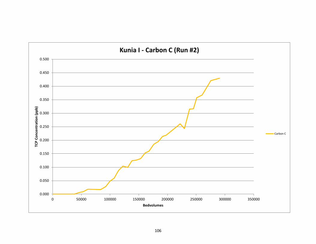
106
0.000
0.050
0.100
0.150
0.200
0.250
0.300
0.350
0.400
0.450
0.500
0 50000 100000 150000 200000 250000 300000 350000
TCP
Conc
entr
atio
n (p
pb)
Bedvolumes
Kunia I - Carbon C (Run #2)
Carbon C

107
7.2.2 GAC Run #3
Run #3 Kunia I
Carbon A/B, D, E, F A/B 5.1 mL/min Sample ID TCP Conc.
(ppb) D 6.63 mL/min E 6.63 mL/min K-Infl1 0.799 F 6.63 mL/min K-Infl2 0.792
Bed Volume 0.355 mL K-Infl3 0.790
TCP Influent 0.794 ppb Influent
Avg. 0.794
mg TCP Mass Adsorbed per kg GAC Mass (mg/kg)
Bed - Volumes
1% Breakthrough
(ppb)
5% Breakthrough
(ppb)
10% Breakthrough
(ppb)
1%
Breakthrough (ppb)
5% Breakthrough
(ppb)
10% Breakthrough
(ppb) Limit Conc.
(ppb) 0.0079 0.0397 0.0794 Limit Conc.
(ppb) 0.0079 0.0397 0.0794
A/B 2.554E-04 3.090E-04 3.433E-04 A/B 161229 196004 219659 D 2.040E-04 2.843E-04 3.037E-04 D 128820 181160 194532 E 1.029E-04 1.705E-04 2.084E-04 E 64960 108739 134780 F 8.999E-05 1.656E-04 2.114E-04 F 56787 106151 137539
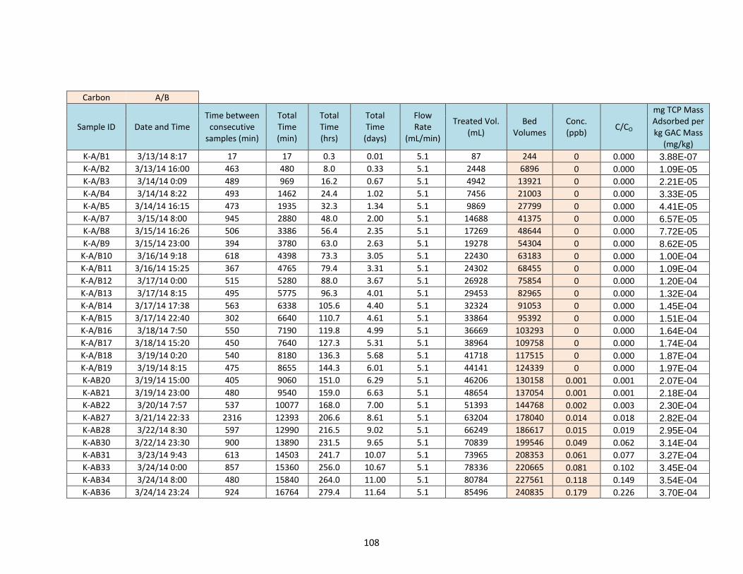
108
Carbon A/B
Sample ID Date and Time Time between
consecutive samples (min)
Total Time (min)
Total Time (hrs)
Total Time
(days)
Flow Rate
(mL/min)
Treated Vol. (mL)
Bed Volumes
Conc. (ppb) C/CO
mg TCP Mass Adsorbed per kg GAC Mass
(mg/kg) K-A/B1 3/13/14 8:17 17 17 0.3 0.01 5.1 87 244 0 0.000 3.88E-07 K-A/B2 3/13/14 16:00 463 480 8.0 0.33 5.1 2448 6896 0 0.000 1.09E-05 K-A/B3 3/14/14 0:09 489 969 16.2 0.67 5.1 4942 13921 0 0.000 2.21E-05 K-A/B4 3/14/14 8:22 493 1462 24.4 1.02 5.1 7456 21003 0 0.000 3.33E-05 K-A/B5 3/14/14 16:15 473 1935 32.3 1.34 5.1 9869 27799 0 0.000 4.41E-05 K-A/B7 3/15/14 8:00 945 2880 48.0 2.00 5.1 14688 41375 0 0.000 6.57E-05 K-A/B8 3/15/14 16:26 506 3386 56.4 2.35 5.1 17269 48644 0 0.000 7.72E-05 K-A/B9 3/15/14 23:00 394 3780 63.0 2.63 5.1 19278 54304 0 0.000 8.62E-05
K-A/B10 3/16/14 9:18 618 4398 73.3 3.05 5.1 22430 63183 0 0.000 1.00E-04 K-A/B11 3/16/14 15:25 367 4765 79.4 3.31 5.1 24302 68455 0 0.000 1.09E-04 K-A/B12 3/17/14 0:00 515 5280 88.0 3.67 5.1 26928 75854 0 0.000 1.20E-04 K-A/B13 3/17/14 8:15 495 5775 96.3 4.01 5.1 29453 82965 0 0.000 1.32E-04 K-A/B14 3/17/14 17:38 563 6338 105.6 4.40 5.1 32324 91053 0 0.000 1.45E-04 K-A/B15 3/17/14 22:40 302 6640 110.7 4.61 5.1 33864 95392 0 0.000 1.51E-04 K-A/B16 3/18/14 7:50 550 7190 119.8 4.99 5.1 36669 103293 0 0.000 1.64E-04 K-A/B17 3/18/14 15:20 450 7640 127.3 5.31 5.1 38964 109758 0 0.000 1.74E-04 K-A/B18 3/19/14 0:20 540 8180 136.3 5.68 5.1 41718 117515 0 0.000 1.87E-04 K-A/B19 3/19/14 8:15 475 8655 144.3 6.01 5.1 44141 124339 0 0.000 1.97E-04 K-AB20 3/19/14 15:00 405 9060 151.0 6.29 5.1 46206 130158 0.001 0.001 2.07E-04 K-AB21 3/19/14 23:00 480 9540 159.0 6.63 5.1 48654 137054 0.001 0.001 2.18E-04 K-AB22 3/20/14 7:57 537 10077 168.0 7.00 5.1 51393 144768 0.002 0.003 2.30E-04 K-AB27 3/21/14 22:33 2316 12393 206.6 8.61 5.1 63204 178040 0.014 0.018 2.82E-04 K-AB28 3/22/14 8:30 597 12990 216.5 9.02 5.1 66249 186617 0.015 0.019 2.95E-04 K-AB30 3/22/14 23:30 900 13890 231.5 9.65 5.1 70839 199546 0.049 0.062 3.14E-04 K-AB31 3/23/14 9:43 613 14503 241.7 10.07 5.1 73965 208353 0.061 0.077 3.27E-04 K-AB33 3/24/14 0:00 857 15360 256.0 10.67 5.1 78336 220665 0.081 0.102 3.45E-04 K-AB34 3/24/14 8:00 480 15840 264.0 11.00 5.1 80784 227561 0.118 0.149 3.54E-04 K-AB36 3/24/14 23:24 924 16764 279.4 11.64 5.1 85496 240835 0.179 0.226 3.70E-04

109
Carbon D
Sample ID Date and Time Time between
consecutive samples (min)
Total Time (min)
Total Time (hrs)
Total Time
(days)
Flow Rate
(mL/min)
Treated Vol. (mL)
Bed Volumes
Conc. (ppb) C/CO
mg TCP Mass Adsorbed per kg GAC Mass
(mg/kg)
K-D1 3/13/14 8:09 9 9 0.2 0.01 6.63 60 168 0 0.000 2.66806E-
07 K-D2 3/13/14 16:00 471 480 8.0 0.33 6.63 3182 8965 0 0.000 1.42E-05 K-D3 3/14/14 0:09 489 969 16.1 0.67 6.63 6424 18097 0 0.000 2.87E-05 K-D4 3/14/14 8:22 493 1462 24.4 1.02 6.63 9693 27304 0 0.000 4.33E-05 K-D5 3/14/14 16:15 473 1935 32.3 1.34 6.63 12829 36138 0 0.000 5.74E-05 K-D6 3/15/14 0:00 465 2400 40.0 1.67 6.63 15912 44823 0 0.000 7.11E-05 K-D7 3/15/14 8:00 480 2880 48.0 2.00 6.63 19094 53787 0 0.000 8.54E-05 K-D8 3/15/14 16:26 506 3386 56.4 2.35 6.63 22449 63237 0 0.000 1.00E-04 K-D9 3/15/14 23:00 394 3780 63.0 2.63 6.63 25061 70595 0 0.000 1.12E-04
K-D10 3/16/14 9:18 618 4398 73.3 3.05 6.63 29159 82137 0.001 0.001 1.30E-04 K-D11 3/16/14 15:25 367 4765 79.4 3.31 6.63 31592 88991 0.001 0.001 1.41E-04 K-D12 3/17/14 0:00 515 5280 88.0 3.67 6.63 35006 98610 0.002 0.003 1.56E-04 K-D13 3/17/14 8:15 495 5775 96.2 4.01 6.63 38288 107854 0.004 0.005 1.71E-04 K-D14 3/17/14 17:38 563 6338 105.6 4.40 6.63 42021 118369 0.006 0.008 1.88E-04 K-D15 3/17/14 22:40 302 6640 110.7 4.61 6.63 44023 124009 0.007 0.009 1.96E-04 K-D16 3/18/14 7:50 550 7190 119.8 4.99 6.63 47670 134281 0.009 0.011 2.13E-04 K-D17 3/18/14 15:20 450 7640 127.3 5.31 6.63 50653 142685 0.019 0.024 2.26E-04 K-D18 3/19/14 0:20 540 8180 136.3 5.68 6.63 54233 152770 0.022 0.028 2.41E-04 K-D19 3/19/14 8:15 475 8655 144.2 6.01 6.63 57383 161641 0.029 0.037 2.55E-04 K-D20 3/19/14 15:00 405 9060 151.0 6.29 6.63 60068 169205 0.032 0.040 2.66E-04 K-D21 3/19/14 23:00 480 9540 159.0 6.63 6.63 63250 178170 0.037 0.047 2.80E-04 K-D22 3/20/14 7:57 537 10077 168.0 7.00 6.63 66811 188199 0.046 0.058 2.95E-04 K-D23 3/20/14 16:15 498 10575 176.3 7.34 6.63 70112 197499 0.095 0.120 3.08E-04 K-D24 3/21/14 1:04 529 11104 185.1 7.71 6.63 73620 207379 0.113 0.142 3.21E-04 K-D25 3/21/14 8:43 459 11563 192.7 8.03 6.63 76663 215951 0.198 0.249 3.32E-04 K-D26 3/21/14 16:00 437 12000 200.0 8.33 6.63 79560 224113 0.192 0.242 3.41E-04 K-D30 3/22/14 23:30 1890 13890 231.5 9.65 6.63 92091 259410 0.220 0.277 3.82E-04 K-D31 3/23/14 9:43 613 14503 241.7 10.07 6.63 96155 270859 0.264 0.333 3.94E-04 K-D32 3/23/14 16:00 377 14880 248.0 10.33 6.63 98654 277900 0.308 0.388 4.01E-04
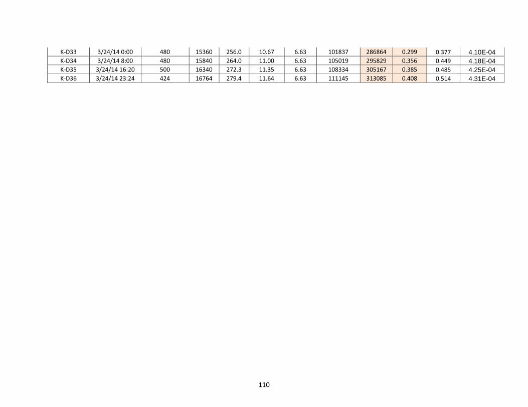
110
K-D33 3/24/14 0:00 480 15360 256.0 10.67 6.63 101837 286864 0.299 0.377 4.10E-04 K-D34 3/24/14 8:00 480 15840 264.0 11.00 6.63 105019 295829 0.356 0.449 4.18E-04 K-D35 3/24/14 16:20 500 16340 272.3 11.35 6.63 108334 305167 0.385 0.485 4.25E-04 K-D36 3/24/14 23:24 424 16764 279.4 11.64 6.63 111145 313085 0.408 0.514 4.31E-04

111
Carbon E
Sample ID Date and Time Time between
consecutive samples (min)
Total Time (min)
Total Time (hrs)
Total Time
(days)
Flow Rate
(mL/min)
Treated Vol. (mL)
Bed Volumes
Conc. (ppb) C/CO
mg TCP Mass Adsorbed per kg GAC Mass
(mg/kg)
K-E1 3/13/14 8:09 9 9 0.2 0.01 6.63 60 168 0 0.000 2.66806E-
07 K-E2 3/13/14 16:00 471 480 8.0 0.33 6.63 3182 8965 0 0.000 1.42E-05 K-E3 3/14/14 0:09 489 969 16.1 0.67 6.63 6424 18097 0 0.000 2.87E-05 K-E4 3/14/14 8:22 493 1462 24.4 1.02 6.63 9693 27304 0 0.000 4.33E-05 K-E5 3/14/14 16:15 473 1935 32.3 1.34 6.63 12829 36138 0 0.000 5.74E-05 K-E6 3/15/14 0:00 465 2400 40.0 1.67 6.63 15912 44823 0 0.000 7.11E-05 K-E7 3/15/14 8:00 480 2880 48.0 2.00 6.63 19094 53787 0 0.000 8.54E-05 K-E8 3/15/14 16:26 506 3386 56.4 2.35 6.63 22449 63237 0.007 0.009 1.00E-04 K-E9 3/15/14 23:00 394 3780 63.0 2.63 6.63 25061 70595 0.011 0.014 1.12E-04
K-E10 3/16/14 9:18 618 4398 73.3 3.05 6.63 29159 82137 0.010 0.013 1.30E-04 K-E11 3/16/14 15:25 367 4765 79.4 3.31 6.63 31592 88991 0.024 0.030 1.40E-04 K-E12 3/17/14 0:00 515 5280 88.0 3.67 6.63 35006 98610 0.022 0.028 1.55E-04 K-E13 3/17/14 8:15 495 5775 96.2 4.01 6.63 38288 107854 0.038 0.048 1.69E-04 K-E14 3/17/14 17:38 563 6338 105.6 4.40 6.63 42021 118369 0.058 0.073 1.85E-04 K-E15 3/17/14 22:40 302 6640 110.7 4.61 6.63 44023 124009 0.061 0.077 1.93E-04 K-E16 3/18/14 7:50 550 7190 119.8 4.99 6.63 47670 134281 0.078 0.098 2.08E-04 K-E17 3/18/14 15:20 450 7640 127.3 5.31 6.63 50653 142685 0.101 0.127 2.19E-04 K-E18 3/19/14 0:20 540 8180 136.3 5.68 6.63 54233 152770 0.121 0.152 2.33E-04 K-E19 3/19/14 8:15 475 8655 144.2 6.01 6.63 57383 161641 0.123 0.155 2.45E-04 K-E22 3/20/14 7:57 1422 10077 168.0 7.00 6.63 66811 188199 0.140 0.176 2.79E-04 K-E23 3/20/14 16:15 498 10575 176.3 7.34 6.63 70112 197499 0.258 0.325 2.89E-04 K-E24 3/21/14 1:04 529 11104 185.1 7.71 6.63 73620 207379 0.265 0.334 3.00E-04 K-E25 3/21/14 8:43 459 11563 192.7 8.03 6.63 76663 215951 0.277 0.349 3.09E-04 K-E27 3/21/14 22:33 830 12393 206.5 8.61 6.63 82166 231452 0.289 0.364 3.24E-04 K-E28 3/22/14 8:30 597 12990 216.5 9.02 6.63 86124 242602 0.285 0.359 3.36E-04 K-E30 3/22/14 23:30 900 13890 231.5 9.65 6.63 92091 259410 0.333 0.420 3.51E-04 K-E31 3/23/14 9:43 613 14503 241.7 10.07 6.63 96155 270859 0.349 0.440 3.61E-04 K-E33 3/24/14 0:00 857 15360 256.0 10.67 6.63 101837 286864 0.358 0.451 3.75E-04 K-E34 3/24/14 8:00 480 15840 264.0 11.00 6.63 105019 295829 0.372 0.469 3.83E-04 K-E36 3/24/14 23:24 924 16764 279.4 11.64 6.63 111145 313085 0.444 0.559 3.95E-04

112
Carbon F
Sample ID Date and Time Time between
consecutive samples (min)
Total Time (min)
Total Time (hrs)
Total Time
(days)
Flow Rate
(mL/min)
Treated Vol. (mL)
Bed Volumes
Conc. (ppb) C/CO
mg TCP Mass Adsorbed per kg GAC Mass
(mg/kg)
K-F1 3/13/14 8:09 9 9 0.2 0.01 6.63 60 168 0 0.000 2.66806E-
07 K-F2 3/13/14 16:00 471 480 8.0 0.33 6.63 3182 8965 0 0.000 1.42E-05 K-F3 3/14/14 0:09 489 969 16.1 0.67 6.63 6424 18097 0 0.000 2.87E-05 K-F4 3/14/14 8:22 493 1462 24.4 1.02 6.63 9693 27304 0 0.000 4.33E-05 K-F5 3/14/14 16:15 473 1935 32.3 1.34 6.63 12829 36138 0 0.000 5.74E-05 K-F6 3/15/14 0:00 465 2400 40.0 1.67 6.63 15912 44823 0 0.000 7.11E-05 K-F7 3/15/14 8:00 480 2880 48.0 2.00 6.63 19094 53787 0 0.000 8.54E-05 K-F8 3/15/14 16:26 506 3386 56.4 2.35 6.63 22449 63237 0.025 0.031 9.99E-05 K-F9 3/15/14 23:00 394 3780 63.0 2.63 6.63 25061 70595 0.032 0.040 1.11E-04
K-F10 3/16/14 9:18 618 4398 73.3 3.05 6.63 29159 82137 0.018 0.023 1.29E-04 K-F11 3/16/14 15:25 367 4765 79.4 3.31 6.63 31592 88991 0.030 0.038 1.39E-04 K-F12 3/17/14 0:00 515 5280 88.0 3.67 6.63 35006 98610 0.025 0.031 1.54E-04 K-F13 3/17/14 8:15 495 5775 96.2 4.01 6.63 38288 107854 0.043 0.054 1.68E-04 K-F15 3/17/14 22:40 865 6640 110.7 4.61 6.63 44023 124009 0.056 0.071 1.92E-04 K-F16 3/18/14 7:50 550 7190 119.8 4.99 6.63 47670 134281 0.072 0.091 2.07E-04 K-F17 3/18/14 15:20 450 7640 127.3 5.31 6.63 50653 142685 0.091 0.115 2.19E-04 K-F18 3/19/14 0:20 540 8180 136.3 5.68 6.63 54233 152770 0.103 0.130 2.33E-04 K-F20 3/19/14 15:00 880 9060 151.0 6.29 6.63 60068 169205 0.118 0.149 2.55E-04 K-F21 3/19/14 23:00 480 9540 159.0 6.63 6.63 63250 178170 0.124 0.156 2.67E-04 K-F22 3/20/14 7:57 537 10077 168.0 7.00 6.63 66811 188199 0.142 0.179 2.80E-04 K-F23 3/20/14 16:15 498 10575 176.3 7.34 6.63 70112 197499 0.234 0.295 2.90E-04 K-F25 3/21/14 8:43 988 11563 192.7 8.03 6.63 76663 215951 0.255 0.321 3.10E-04 K-F27 3/21/14 22:33 830 12393 206.5 8.61 6.63 82166 231452 0.243 0.306 3.27E-04 K-F30 3/22/14 23:30 1497 13890 231.5 9.65 6.63 92091 259410 0.294 0.370 3.55E-04 K-F32 3/23/14 16:00 990 14880 248.0 10.33 6.63 98654 277900 0.332 0.418 3.72E-04 K-F35 3/24/14 16:20 1460 16340 272.3 11.35 6.63 108334 305167 0.329 0.415 3.98E-04 K-F36 3/24/14 23:24 424 16764 279.4 11.64 6.63 111145 313085 0.414 0.522 4.04E-04

113
0
0.05
0.1
0.15
0.2
0.25
0.3
0.35
0.4
0.45
0.5
0 50000 100000 150000 200000 250000 300000 350000
TCP
Conc
entr
atio
n (p
pb)
Bedvolumes
Kunia I - Carbon A/B, D, E, F (Run #3)
Carbon A/B
Carbon D
Carbon E
Carbon F

114
7.2.3 GAC Run #4
Run #4 Waipahu #3
Carbon D, E, F Sample TCP Conc. (ppb) D 5.66 mL/min
E 5.66 mL/min W_Inf1 0.517 F 4.35 mL/min W_Inf2 0.536
Bed Volume 0.355 mL W_Inf3 0.608
TCP Influent 0.641 ppb Influent
Avg. 0.554
mg TCP Mass Adsorbed per kg GAC Mass (mg/kg)
Bed - Volumes
1% Breakthrough
(ppb)
5% Breakthough
(ppb)
10% Breakthru
(ppb)
1%
Breakthrough (ppb)
5% Breakthough
(ppb)
10% Breakthru
(ppb) Limit Conc.
(ppb) 0.0064 0.0321 0.0641 Limit Conc.
(ppb) 0.0064 0.0321 0.0641
D 1.764E-04 2.188E-04 2.543E-04 D 159467 199164 234461 E 7.341E-05 1.104E-04 1.978E-04 E 66507 101033 186156 F 1.469E-04 2.016E-04 2.359E-04 F 132957 183896 218547

115
Carbon D
Sample ID Date and Time Time between
consecutive samples (min)
Total Time (min)
Total Time (hrs)
Total Time (days)
Flow Rate (mL/min)
Treated Vol. (mL)
Bed Volumes
Conc. (ppb) C/CO
mg TCP Mass Adsorbed per kg GAC Mass
(mg/kg) W-D1 4/7/14 15:45 0 0 0.0 0.0 6.54 0 0 0.000 0.000 0 W-D2 4/7/14 23:35 470 470 7.8 0.3 6.54 3074 8659 0.000 0.000 9.59E-06 W-D3 4/8/14 8:07 512 982 16.4 0.7 6.68 6494 18293 0.000 0.000 2.03E-05 W-D4 4/8/14 14:47 400 1382 23.0 1.0 6.13 8946 25200 0.000 0.000 2.79E-05 W-D5 4/8/14 23:40 533 1915 31.9 1.3 5.58 11920 33578 0.000 0.000 3.72E-05 W-D6 4/9/14 8:25 525 2440 40.7 1.7 5.62 14871 41889 0.000 0.000 4.64E-05 W-D8 4/9/14 23:20 895 3335 55.6 2.3 5.62 19900 56058 0.000 0.000 6.21E-05
W-D10 4/10/14 14:46 926 4261 71.0 3.0 5.62 25105 70717 0.001 0.002 7.83E-05 W-D11 4/10/14 22:25 459 4720 78.7 3.3 5.45 27606 77764 0.000 0.000 8.61E-05 W-D12 4/11/14 8:20 595 5315 88.6 3.7 5.45 30849 86898 0.000 0.000 9.63E-05 W-D13 4/11/14 13:45 325 5640 94.0 3.9 5.45 32620 91888 0.000 0.000 1.02E-04 W-D14 4/11/14 23:45 600 6240 104.0 4.3 5.45 35890 101099 0.000 0.000 1.12E-04 W-D15 4/12/14 9:12 567 6807 113.4 4.7 5.45 38980 109804 0.000 0.000 1.22E-04 W-D16 4/12/14 15:43 391 7198 120.0 5.0 5.20 41014 115531 0.000 0.000 1.28E-04 W-D17 4/12/14 22:43 420 7618 127.0 5.3 5.20 43198 121683 0.001 0.002 1.35E-04 W-D18 4/13/14 10:19 696 8314 138.6 5.8 5.20 46817 131878 0.001 0.002 1.46E-04 W-D19 4/13/14 15:57 338 8652 144.2 6.0 5.20 48574 136829 0.002 0.004 1.52E-04 W-D20 4/13/14 22:48 411 9063 151.0 6.3 5.20 50712 142849 0.003 0.005 1.58E-04 W-D21 4/14/14 8:33 585 9648 160.8 6.7 5.20 53754 151418 0.004 0.007 1.68E-04 W-D23 4/14/14 23:45 912 10560 176.0 7.3 5.20 58496 164777 0.008 0.014 1.82E-04 W-D24 4/15/14 8:07 502 11062 184.4 7.7 5.20 61106 172130 0.011 0.020 1.90E-04 W-D25 4/15/14 14:45 398 11460 191.0 8.0 5.20 63176 177960 0.013 0.023 1.96E-04 W-D26 4/15/14 22:49 484 11944 199.1 8.3 5.54 65857 185513 0.023 0.042 2.04E-04 W-D27 4/16/14 9:45 656 12600 210.0 8.8 5.54 69492 195751 0.028 0.051 2.15E-04 W-D28 4/16/14 15:09 324 12924 215.4 9.0 5.54 71286 200807 0.034 0.061 2.21E-04 W_D29 4/16/14 23:10 481 13405 223.4 9.3 5.54 73951 208313 0.041 0.074 2.28E-04 W_D30 4/17/14 8:28 558 13963 232.7 9.7 5.54 77043 217021 0.043 0.078 2.37E-04 W_D31 4/17/14 15:39 431 14394 239.9 10.0 5.54 79430 223747 0.053 0.096 2.44E-04 W_D32 4/17/14 23:20 461 14855 247.6 10.3 5.54 81984 230941 0.059 0.106 2.51E-04 W_D34 4/18/14 15:33 973 15828 263.8 11.0 5.54 87375 246126 0.081 0.146 2.65E-04 W_D35 4/18/14 22:07 394 16222 270.4 11.3 5.54 89557 252274 0.076 0.137 2.71E-04

116
W-D37 4/19/14 18:16 1209 17431 290.5 12.1 5.54 96255 271142 0.122 0.220 2.88E-04 W-D38 4/19/14 23:26 310 17741 295.7 12.3 5.54 97973 275979 0.131 0.236 2.92E-04 W-D39 4/20/14 7:51 505 18246 304.1 12.7 5.54 100770 283860 0.155 0.280 2.98E-04 W-D40 4/20/14 17:02 551 18797 313.3 13.1 5.54 103823 292459 0.184 0.332 3.04E-04 W-D41 4/20/14 22:50 348 19145 319.1 13.3 5.54 105751 297890 0.186 0.336 3.08E-04 W-D42 4/21/14 8:18 568 19713 328.5 13.7 5.54 108898 306754 0.216 0.390 3.14E-04 W-D43 4/21/14 17:24 546 20259 337.6 14.1 5.54 111922 315274 0.241 0.435 3.20E-04 W-D44 4/21/14 23:07 343 20602 343.4 14.3 5.54 113823 320627 0.252 0.455 3.23E-04 W-D46 4/22/14 14:44 937 21539 359.0 15.0 5.54 119014 335250 0.297 0.536 3.30E-04

117
Carbon E
Sample ID Date and Time Time between
consecutive samples (min)
Total Time (min)
Total Time (hrs)
Total Time (days)
Flow Rate (mL/min)
Treated Vol. (mL)
Bed Volumes
Conc. (ppb) C/CO
mg TCP Mass Adsorbed per kg GAC Mass
(mg/kg) W-E1 4/7/14 15:45 0 0 0.0 0.0 6.54 0 0 0.000 0.000 0 W-E2 4/7/14 23:35 470 470 7.8 0.3 6.54 3074 8659 0.000 0.000 9.59E-06 W-E3 4/8/14 8:07 512 982 16.4 0.7 6.46 6381 17976 0.001 0.002 1.99E-05 W-E4 4/8/14 14:47 400 1382 23.0 1.0 6.09 8817 24838 0.001 0.002 2.75E-05 W-E5 4/8/14 23:40 533 1915 31.9 1.3 5.74 11877 33456 0.002 0.004 3.70E-05 W-E6 4/9/14 8:25 525 2440 40.7 1.7 5.67 14853 41841 0.000 0.000 4.63E-05 W-E7 4/9/14 15:09 404 2844 47.4 2.0 5.67 17144 48293 0.002 0.004 5.34E-05 W-E8 4/9/14 23:20 491 3335 55.6 2.3 5.62 19904 56066 0.000 0.000 6.20E-05
W-E10 4/10/14 14:46 926 4261 71.0 3.0 5.62 25108 70726 0.009 0.016 7.80E-05 W-E11 4/10/14 22:25 459 4720 78.7 3.3 5.58 27669 77941 0.018 0.032 8.57E-05 W-E12 4/11/14 8:20 595 5315 88.6 3.7 5.58 30989 87293 0.014 0.025 9.58E-05 W-E13 4/11/14 13:45 325 5640 94.0 3.9 5.58 32803 92401 0.011 0.020 1.01E-04 W-E14 4/11/14 23:45 600 6240 104.0 4.3 5.58 36151 101832 0.034 0.061 1.11E-04 W-E15 4/12/14 9:12 567 6807 113.4 4.7 5.65 39354 110857 0.025 0.045 1.21E-04 W-E16 4/12/14 15:43 391 7198 120.0 5.0 5.65 41563 117080 0.024 0.043 1.27E-04 W-E17 4/12/14 22:43 420 7618 127.0 5.3 5.65 43936 123764 0.031 0.056 1.34E-04 W-E18 4/13/14 10:19 696 8314 138.6 5.8 5.65 47869 134841 0.040 0.072 1.46E-04 W-E19 4/13/14 15:57 338 8652 144.2 6.0 5.65 49778 140221 0.045 0.081 1.51E-04 W-E20 4/13/14 22:48 411 9063 151.0 6.3 5.65 52100 146762 0.048 0.087 1.58E-04 W-E21 4/14/14 8:33 585 9648 160.8 6.7 5.65 55406 156072 0.031 0.056 1.68E-04 W-E22 4/14/14 16:05 452 10100 168.3 7.0 5.65 57960 163266 0.040 0.072 1.75E-04 W-E23 4/14/14 23:45 460 10560 176.0 7.3 5.65 60559 170587 0.046 0.083 1.82E-04 W-E24 4/15/14 8:07 502 11062 184.4 7.7 5.65 63395 178577 0.055 0.099 1.90E-04 W-E25 4/15/14 14:45 398 11460 191.0 8.0 5.65 65644 184911 0.062 0.112 1.97E-04 W-E26 4/15/14 22:49 484 11944 199.1 8.3 5.65 68378 192614 0.075 0.135 2.04E-04 W-E27 4/16/14 9:45 656 12600 210.0 8.8 5.65 72085 203055 0.080 0.144 2.14E-04 W-E28 4/16/14 15:09 324 12924 215.4 9.0 5.65 73915 208212 0.083 0.150 2.19E-04 W-E29 4/16/14 23:10 481 13405 223.4 9.3 5.65 76633 215867 0.092 0.166 2.26E-04 W_E30 4/17/14 8:28 558 13963 232.7 9.7 5.65 79785 224748 0.096 0.173 2.34E-04 W_E31 4/17/14 15:39 431 14394 239.9 10.0 5.65 82221 231607 0.100 0.181 2.40E-04 W_E32 4/17/14 23:20 461 14855 247.6 10.3 5.65 84825 238944 0.108 0.195 2.47E-04

118
W_E33 4/18/14 8:02 522 15377 256.3 10.7 5.65 87775 247252 0.125 0.226 2.54E-04 W_E34 4/18/14 15:33 451 15828 263.8 11.0 5.65 90323 254430 0.142 0.256 2.60E-04 W_E35 4/18/14 22:07 394 16222 270.4 11.3 5.65 92549 260701 0.140 0.253 2.65E-04 W-E36 4/19/14 8:31 624 16846 280.8 11.7 5.65 96074 270632 0.183 0.330 2.72E-04 W-E37 4/19/14 18:16 585 17431 290.5 12.1 5.65 99380 279943 0.163 0.294 2.80E-04 W-E38 4/19/14 23:26 310 17741 295.7 12.3 5.65 101131 284877 0.172 0.310 2.83E-04 W-E39 4/20/14 7:51 505 18246 304.1 12.7 5.65 103984 292914 0.192 0.347 2.89E-04 W-E41 4/20/14 22:50 899 19145 319.1 13.3 5.65 109064 307222 0.200 0.361 2.99E-04 W-E42 4/21/14 8:18 568 19713 328.5 13.7 5.65 112273 316262 0.213 0.384 3.05E-04 W-E43 4/21/14 17:24 546 20259 337.6 14.1 5.65 115358 324952 0.228 0.412 3.11E-04 W-E44 4/21/14 23:07 343 20602 343.4 14.3 5.65 117296 330411 0.227 0.410 3.15E-04 W-E45 4/22/14 8:32 565 21167 352.8 14.7 5.65 120488 339403 0.233 0.421 3.20E-04 W-E46 4/22/14 14:44 372 21539 359.0 15.0 5.65 122590 345324 0.242 0.437 3.24E-04

119
Carbon F
Sample ID Date and Time Time between
consecutive samples (min)
Total Time (min)
Total Time (hrs)
Total Time (days)
Flow Rate (mL/min)
Treated Vol. (mL)
Bed Volumes
Conc. (ppb) C/CO
mg TCP Mass Adsorbed per kg GAC Mass
(mg/kg) W-F1 4/7/14 15:45 0 0 0.0 0.0 4.57 0 0 0.000 0.000 0 W-F2 4/7/14 23:35 470 470 7.8 0.3 4.57 2148 6050 0.001 0.002 6.69E-06 W-F3 4/8/14 8:07 512 982 16.4 0.7 4.37 4385 12353 0.000 0.000 1.37E-05 W-F4 4/8/14 14:47 400 1382 23.0 1.0 4.38 6137 17288 0.000 0.000 1.91E-05 W-F5 4/8/14 23:40 533 1915 31.9 1.3 4.40 8483 23894 0.000 0.000 2.65E-05 W-F6 4/9/14 8:25 525 2440 40.7 1.7 3.98 10572 29780 0.000 0.000 3.30E-05 W-F7 4/9/14 15:09 404 2844 47.4 2.0 4.00 12188 34333 0.000 0.000 3.80E-05 W-F8 4/9/14 23:20 491 3335 55.6 2.3 4.00 14152 39865 0.000 0.000 4.42E-05
W-F10 4/10/14 14:46 926 4261 71.0 3.0 4.37 18199 51264 0.001 0.002 5.68E-05 W-F11 4/10/14 22:25 459 4720 78.7 3.3 4.39 20214 56940 0.000 0.000 6.31E-05 W-F12 4/11/14 8:20 595 5315 88.6 3.7 4.39 22826 64298 0.000 0.000 7.12E-05 W-F13 4/11/14 13:45 325 5640 94.0 3.9 4.39 24252 68317 0.000 0.000 7.57E-05 W-F14 4/11/14 23:45 600 6240 104.0 4.3 4.39 26886 75737 0.000 0.000 8.39E-05 W-F15 4/12/14 9:12 567 6807 113.4 4.7 4.39 29376 82748 0.001 0.002 9.16E-05 W-F16 4/12/14 15:43 391 7198 120.0 5.0 4.34 31073 87528 0.000 0.000 9.69E-05 W-F17 4/12/14 22:43 420 7618 127.0 5.3 4.34 32895 92663 0.002 0.004 1.03E-04 W-F18 4/13/14 10:19 696 8314 138.6 5.8 4.34 35916 101172 0.003 0.005 1.12E-04 W-F19 4/13/14 15:57 338 8652 144.2 6.0 4.34 37383 105304 0.003 0.005 1.17E-04 W-F20 4/13/14 22:48 411 9063 151.0 6.3 4.34 39167 110329 0.004 0.007 1.22E-04 W-F21 4/14/14 8:33 585 9648 160.8 6.7 4.34 41706 117480 0.005 0.009 1.30E-04 W-F22 4/14/14 16:05 452 10100 168.3 7.0 4.34 43667 123006 0.005 0.009 1.36E-04 W-F23 4/14/14 23:45 460 10560 176.0 7.3 4.34 45664 128630 0.005 0.009 1.42E-04 W-F24 4/15/14 8:07 502 11062 184.4 7.7 4.34 47842 134767 0.007 0.013 1.49E-04 W-F25 4/15/14 14:45 398 11460 191.0 8.0 4.34 49570 139633 0.005 0.009 1.54E-04 W-F26 4/15/14 22:49 484 11944 199.1 8.3 4.34 51670 145550 0.011 0.020 1.61E-04 W-F27 4/16/14 9:45 656 12600 210.0 8.8 4.34 54517 153570 0.011 0.020 1.69E-04 W-F28 4/16/14 15:09 324 12924 215.4 9.0 4.34 55923 157531 0.014 0.025 1.74E-04 W-F29 4/16/14 23:10 481 13405 223.4 9.3 4.34 58011 163411 0.018 0.032 1.80E-04 W_F30 4/17/14 8:28 558 13963 232.7 9.7 4.34 60433 170233 0.020 0.036 1.87E-04 W_F31 4/17/14 15:39 431 14394 239.9 10.0 4.34 62303 175502 0.025 0.045 1.93E-04

120
W_F32 4/17/14 23:20 461 14855 247.6 10.3 4.34 64304 181138 0.026 0.047 1.99E-04 W_F33 4/18/14 8:02 522 15377 256.3 10.7 4.34 66569 187519 0.040 0.072 2.05E-04 W_F34 4/18/14 15:33 451 15828 263.8 11.0 4.34 68527 193033 0.038 0.069 2.11E-04 W_F35 4/18/14 22:07 394 16222 270.4 11.3 4.34 70237 197850 0.042 0.076 2.16E-04 W-F36 4/19/14 8:31 624 16846 280.8 11.7 4.34 72945 205478 0.088 0.159 2.23E-04 W-F37 4/19/14 18:16 585 17431 290.5 12.1 4.34 75484 212630 0.059 0.106 2.30E-04 W-F38 4/19/14 23:26 310 17741 295.7 12.3 4.34 76829 216420 0.061 0.110 2.34E-04 W-F39 4/20/14 7:51 505 18246 304.1 12.7 4.34 79021 222594 0.070 0.126 2.40E-04 W-F41 4/20/14 22:50 899 19145 319.1 13.3 4.34 82923 233585 0.081 0.146 2.50E-04 W-F42 4/21/14 8:18 568 19713 328.5 13.7 4.34 85388 240529 0.085 0.153 2.57E-04 W-F43 4/21/14 17:24 546 20259 337.6 14.1 4.34 87757 247204 0.092 0.166 2.63E-04 W-F44 4/21/14 23:07 343 20602 343.4 14.3 4.34 89246 251397 0.098 0.177 2.67E-04 W-F45 4/22/14 8:32 565 21167 352.8 14.7 4.34 91698 258304 0.107 0.193 2.73E-04 W-F46 4/22/14 14:44 372 21539 359.0 15.0 4.34 93312 262852 0.147 0.265 2.77E-04

121
0.000
0.050
0.100
0.150
0.200
0.250
0.300
0.350
0 50000 100000 150000 200000 250000 300000 350000 400000
TCP
Conc
entr
atio
n (p
pb)
Bedvolumes
Waipahu III - Carbon D, E, F (Run #4)
Carbon D
Carbon E
Carbon F

122
7.2.4 GAC Run #5
Run #5 Waipahu #3
Carbon A/B, C, G Sample TCP Conc. (ppb) A/B 4.35 mL/min
C 9.67 mL/min W-Inf1 0.517 G 4.35 mL/min W-Inf2 0.536
Bed Volume 0.355 mL W-Inf3 0.608
TCP Influent 0.554 ppb Influent
Avg. 0.554
mg TCP Mass Adsorbed per kg GAC Mass (mg/kg)
Bed - Volumes
1% Breakthru
(ppb)
5% Breakthru
(ppb)
10% Breakthru
(ppb)
1%
Breakthru (ppb)
5% Breakthru
(ppb)
10% Breakthru
(ppb) Limit Conc.
(ppb) 0.0055 0.0277 0.0554 Limit Conc.
(ppb) 0.0055 0.0277 0.0554
A/B 2.642E-04 3.270E-04 3.762E-04 A/B 238763 296847 344999 C 7.199E-05 1.196E-04 1.386E-04 C 65147 109268 128116 G 1.932E-04 2.414E-04 2.813E-04 G 174595 219551 258980

123
Carbon A/B
Sample ID Date and Time Time between
consecutive samples (min)
Total Time (min)
Total Time (hrs)
Total Time
(days)
Flow Rate (mL/min)
Treated Vol. (mL)
Bed Volumes Conc. (ppb) C/CO
mg TCP Mass Adsorbed per kg GAC Mass
(mg/kg) W-A/B1 5/1/14 16:11 0 0 0.0 0.0 3.81 0 0 0.000 0.000 0 W-A/B2 5/1/14 22:07 356 356 5.9 0.2 3.81 1356 3821 0.000 0.000 4.23E-06 W-A/B3 5/2/14 8:30 623 979 16.3 0.7 3.81 3730 10507 0.000 0.000 1.16E-05 W-A/B4 5/2/14 16:17 467 1446 24.1 1.0 3.81 5509 15519 0.000 0.000 1.72E-05 W-A/B5 5/2/14 22:54 397 1843 30.7 1.3 4.33 7228 20361 0.000 0.000 2.26E-05 W-A/B6 5/3/14 9:27 633 2476 41.3 1.7 4.29 9944 28011 0.000 0.000 3.10E-05 W-A/B7 5/3/14 17:15 468 2944 49.1 2.0 4.29 11952 33666 0.000 0.000 3.73E-05 W-A/B8 5/3/14 23:11 356 3300 55.0 2.3 4.29 13479 37968 0.000 0.000 4.21E-05 W-A/B9 5/4/14 10:04 653 3953 65.9 2.7 4.30 16287 45878 0.000 0.000 5.08E-05
W-A/B10 5/4/14 16:11 367 4320 72.0 3.0 4.30 17865 50323 0.000 0.000 5.58E-05 W-A/B11 5/4/14 22:13 362 4682 78.0 3.3 4.15 19367 54555 0.000 0.000 6.04E-05 W-A/B12 5/5/14 6:58 525 5207 86.8 3.6 4.15 21546 60693 0.000 0.000 6.72E-05 W-A/B13 5/5/14 14:53 475 5682 94.7 3.9 4.15 23517 66245 0.000 0.000 7.34E-05 W-A/B14 5/6/14 9:49 1136 6818 113.6 4.7 4.15 28232 79525 0.000 0.000 8.81E-05 W-A/B15 5/6/14 16:00 371 7189 119.8 5.0 4.15 29771 83862 0.000 0.000 9.29E-05 W-A/B16 5/6/14 22:30 390 7579 126.3 5.3 4.04 31347 88301 0.000 0.000 9.78E-05 W-A/B17 5/7/14 7:03 513 8092 134.9 5.6 4.04 33419 94139 0.000 0.000 1.04E-04 W-A/B18 5/7/14 18:30 687 8779 146.3 6.1 4.04 36195 101957 0.000 0.000 1.13E-04 W-A/B19 5/7/14 22:38 248 9027 150.5 6.3 4.04 37197 104779 0.000 0.000 1.16E-04 W-A/B20 5/8/14 6:56 498 9525 158.8 6.6 4.04 39209 110447 0.002 0.004 1.22E-04 W-A/B21 5/8/14 17:18 622 10147 169.1 7.0 4.04 41721 117525 0.000 0.000 1.30E-04 W-A/B22 5/9/14 8:37 919 11066 184.4 7.7 4.56 45912 129330 0.000 0.000 1.43E-04 W-A/B23 5/9/14 16:00 443 11509 191.8 8.0 4.56 47932 135020 0.000 0.000 1.50E-04 W-A/B25 5/10/14 11:00 1140 12649 210.8 8.8 4.49 53051 149439 0.000 0.000 1.66E-04 W-A/B26 5/10/14 16:00 300 12949 215.8 9.0 4.49 54398 153233 0.000 0.000 1.70E-04 W-A/B27 5/10/14 23:15 435 13384 223.1 9.3 4.51 56360 158760 0.000 0.000 1.76E-04 W-A/B28 5/11/14 9:53 638 14022 233.7 9.7 4.51 59237 166865 0.000 0.000 1.85E-04 W-A/B29 5/11/14 15:48 355 14377 239.6 10.0 4.51 60838 171375 0.000 0.000 1.90E-04 W-A/B30 5/11/14 23:07 439 14816 246.9 10.3 4.51 62818 176952 0.000 0.000 1.96E-04
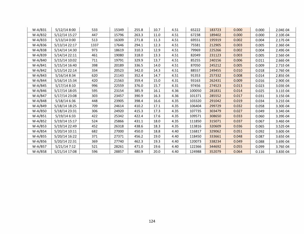
124
W-A/B31 5/12/14 8:00 533 15349 255.8 10.7 4.51 65222 183723 0.000 0.000 2.04E-04 W-A/B32 5/12/14 15:27 447 15796 263.3 11.0 4.51 67238 189402 0.000 0.000 2.10E-04 W-A/B33 5/13/14 0:00 513 16309 271.8 11.3 4.51 69551 195919 0.002 0.004 2.17E-04 W-A/B36 5/13/14 22:17 1337 17646 294.1 12.3 4.51 75581 212905 0.003 0.005 2.36E-04 W-A/B38 5/14/14 14:30 973 18619 310.3 12.9 4.51 79969 225266 0.002 0.004 2.49E-04 W-A/B39 5/14/14 22:11 461 19080 318.0 13.3 4.51 82049 231123 0.003 0.005 2.56E-04 W-A/B40 5/15/14 10:02 711 19791 329.9 13.7 4.51 85255 240156 0.006 0.011 2.66E-04 W-A/B41 5/15/14 16:40 398 20189 336.5 14.0 4.51 87050 245212 0.005 0.009 2.71E-04 W-A/B42 5/15/14 22:14 334 20523 342.0 14.3 4.51 88557 249455 0.010 0.018 2.76E-04 W-A/B43 5/16/14 8:34 620 21143 352.4 14.7 4.51 91353 257332 0.008 0.014 2.85E-04 W-A/B44 5/16/14 15:34 420 21563 359.4 15.0 4.31 93163 262431 0.009 0.016 2.90E-04 W-A/B45 5/17/14 8:10 996 22559 376.0 15.7 4.31 97456 274523 0.013 0.023 3.03E-04 W-A/B46 5/17/14 18:05 595 23154 385.9 16.1 4.36 100050 281831 0.014 0.025 3.11E-04 W-A/B47 5/17/14 23:08 303 23457 390.9 16.3 4.36 101371 285552 0.017 0.031 3.15E-04 W-A/B48 5/18/14 6:36 448 23905 398.4 16.6 4.35 103320 291042 0.019 0.034 3.21E-04 W-A/B49 5/18/14 18:25 709 24614 410.2 17.1 4.35 106404 299729 0.032 0.058 3.30E-04 W-A/B50 5/18/14 23:31 306 24920 415.3 17.3 4.35 107735 303479 0.027 0.049 3.34E-04 W-A/B51 5/19/14 6:33 422 25342 422.4 17.6 4.35 109571 308650 0.033 0.060 3.39E-04 W-A/B52 5/19/14 15:17 524 25866 431.1 18.0 4.35 111850 315071 0.037 0.067 3.46E-04 W-A/B53 5/19/14 22:49 452 26318 438.6 18.3 4.35 113816 320609 0.036 0.065 3.52E-04 W-A/B54 5/20/14 10:11 682 27000 450.0 18.8 4.40 116817 329062 0.051 0.092 3.60E-04 W-A/B55 5/20/14 16:22 371 27371 456.2 19.0 4.40 118450 333661 0.048 0.087 3.65E-04 W-A/B56 5/20/14 22:31 369 27740 462.3 19.3 4.40 120073 338234 0.049 0.088 3.69E-04 W-A/B57 5/21/14 7:12 521 28261 471.0 19.6 4.40 122366 344692 0.055 0.099 3.76E-04 W-A/B58 5/21/14 17:08 596 28857 480.9 20.0 4.40 124988 352079 0.064 0.116 3.83E-04

125
Carbon C
Sample ID Date and Time Time between
consecutive samples (min)
Total Time (min)
Total Time (hrs)
Total Time
(days)
Flow Rate (mL/min)
Treated Vol. (mL)
Bed Volumes Conc. (ppb) C/CO
mg TCP Mass Adsorbed per kg GAC Mass
(mg/kg) W-C1 5/1/14 16:11 0 0 0.0 0.0 9.35 0 0 0.000 0.000 0 W-C2 5/1/14 22:07 356 356 5.9 0.2 9.35 3329 9376 0.000 0.000 1.04E-05 W-C3 5/2/14 8:30 623 979 16.3 0.7 9.35 9154 25785 0.000 0.000 2.86E-05 W-C4 5/2/14 16:17 467 1446 24.1 1.0 9.35 13520 38085 0.000 0.000 4.22E-05 W-C5 5/2/14 22:54 397 1843 30.7 1.3 10.19 17566 49480 0.000 0.000 5.48E-05 W-C6 5/3/14 9:27 633 2476 41.3 1.7 9.52 23592 66455 0.006 0.011 7.34E-05 W-C7 5/3/14 17:15 468 2944 49.1 2.0 9.52 28047 79006 0.000 0.000 8.73E-05 W-C8 5/3/14 23:11 356 3300 55.0 2.3 9.52 31436 88553 0.014 0.025 9.76E-05 W-C9 5/4/14 10:04 653 3953 65.9 2.7 9.64 37731 106285 0.022 0.040 1.17E-04
W-C10 5/4/14 16:11 367 4320 72.0 3.0 9.64 41269 116251 0.041 0.074 1.27E-04 W-C11 5/4/14 22:13 362 4682 78.0 3.3 9.85 44835 126295 0.053 0.096 1.37E-04 W-C12 5/5/14 6:58 525 5207 86.8 3.6 9.85 50006 140862 0.072 0.130 1.51E-04 W-C13 5/5/14 14:53 475 5682 94.7 3.9 9.85 54685 154041 0.087 0.157 1.63E-04 W-C14 5/6/14 9:49 1136 6818 113.6 4.7 9.85 65874 185561 0.163 0.294 1.88E-04 W-C15 5/6/14 16:00 371 7189 119.8 5.0 10.07 69610 196085 0.176 0.318 1.96E-04 W-C16 5/6/14 22:30 390 7579 126.3 5.3 10.07 73538 207148 0.185 0.334 2.04E-04 W-C17 5/7/14 7:03 513 8092 134.9 5.6 10.07 78703 221700 0.207 0.374 2.14E-04 W-C18 5/7/14 18:30 687 8779 146.3 6.1 10.07 85622 241187 0.243 0.439 2.26E-04 W-C19 5/7/14 22:38 248 9027 150.5 6.3 10.07 88119 248222 0.254 0.458 2.30E-04 W-C20 5/8/14 6:56 498 9525 158.8 6.6 10.07 93134 262349 0.253 0.457 2.39E-04 W-C21 5/8/14 17:18 622 10147 169.1 7.0 9.86 99267 279624 0.301 0.543 2.48E-04 W-C22 5/9/14 8:37 919 11066 184.4 7.7 9.86 108328 305149 0.310 0.560 2.60E-04 W-C23 5/9/14 16:00 443 11509 191.8 8.0 9.86 112696 317454 0.316 0.570 2.66E-04 W-C25 5/10/14 11:00 1140 12649 210.8 8.8 9.63 123674 348378 0.315 0.569 2.81E-04 W-C26 5/10/14 16:00 300 12949 215.8 9.0 9.63 126563 356516 0.338 0.610 2.84E-04 W-C27 5/10/14 23:15 435 13384 223.1 9.3 9.63 130752 368316 0.338 0.610 2.89E-04 W-C28 5/11/14 9:53 638 14022 233.7 9.7 9.63 136896 385623 0.339 0.612 2.97E-04 W-C32 5/12/14 15:27 1774 15796 263.3 11.0 4.51 144897 408160 0.379 0.684 3.05E-04

126
Carbon G
Sample ID Date and Time Time between
consecutive samples (min)
Total Time (min)
Total Time (hrs)
Total Time
(days)
Flow Rate (mL/min)
Treated Vol. (mL)
Bed Volumes Conc. (ppb) C/CO
mg TCP Mass Adsorbed per kg GAC Mass
(mg/kg) W-G1 5/1/14 16:11 0 0 0.0 0.0 4.08 0 0 0.000 0.000 0 W-G2 5/1/14 22:07 356 356 5.9 0.2 4.08 1452 4091 0.000 0.000 4.53E-06 W-G3 5/2/14 8:30 623 979 16.3 0.7 4.08 3994 11252 0.000 0.000 1.25E-05 W-G4 5/2/14 16:17 467 1446 24.1 1.0 4.08 5900 16619 0.000 0.000 1.84E-05 W-G5 5/2/14 22:54 397 1843 30.7 1.3 4.43 7658 21573 0.000 0.000 2.39E-05 W-G6 5/3/14 9:27 633 2476 41.3 1.7 4.50 10507 29597 0.000 0.000 3.28E-05 W-G7 5/3/14 17:15 468 2944 49.1 2.0 4.50 12613 35529 0.000 0.000 3.94E-05 W-G8 5/3/14 23:11 356 3300 55.0 2.3 4.50 14215 40042 0.000 0.000 4.44E-05 W-G9 5/4/14 10:04 653 3953 65.9 2.7 4.48 17140 48283 0.000 0.000 5.35E-05
W-G10 5/4/14 16:11 367 4320 72.0 3.0 4.48 18784 52914 0.000 0.000 5.86E-05 W-G11 5/4/14 22:13 362 4682 78.0 3.3 4.38 20370 57380 0.000 0.000 6.36E-05 W-G12 5/5/14 6:58 525 5207 86.8 3.6 4.38 22670 63858 0.000 0.000 7.08E-05 W-G13 5/5/14 14:53 475 5682 94.7 3.9 4.38 24750 69718 0.000 0.000 7.72E-05 W-G14 5/6/14 9:49 1136 6818 113.6 4.7 4.38 29726 83734 0.000 0.000 9.28E-05 W-G15 5/6/14 16:00 371 7189 119.8 5.0 4.38 31351 88312 0.000 0.000 9.78E-05 W-G16 5/6/14 22:30 390 7579 126.3 5.3 4.31 33032 93047 0.000 0.000 1.03E-04 W-G17 5/7/14 7:03 513 8092 134.9 5.6 4.31 35243 99275 0.000 0.000 1.10E-04 W-G18 5/7/14 18:30 687 8779 146.3 6.1 4.31 38204 107616 0.001 0.002 1.19E-04 W-G19 5/7/14 22:38 248 9027 150.5 6.3 4.31 39272 110627 0.001 0.002 1.23E-04 W-G20 5/8/14 6:56 498 9525 158.8 6.6 4.31 41419 116673 0.000 0.000 1.29E-04 W-G21 5/8/14 17:18 622 10147 169.1 7.0 4.31 44100 124224 0.000 0.000 1.38E-04 W-G22 5/9/14 8:37 919 11066 184.4 7.7 4.35 48097 135485 0.002 0.004 1.50E-04 W-G23 5/9/14 16:00 443 11509 191.8 8.0 4.35 50024 140914 0.001 0.002 1.56E-04 W-G25 5/10/14 11:00 1140 12649 210.8 8.8 4.06 54653 153952 0.001 0.002 1.70E-04 W-G26 5/10/14 16:00 300 12949 215.8 9.0 4.06 55871 157383 0.000 0.000 1.74E-04 W-G27 5/10/14 23:15 435 13384 223.1 9.3 4.54 57846 162946 0.003 0.005 1.80E-04 W-G28 5/11/14 9:53 638 14022 233.7 9.7 4.54 60742 171105 0.004 0.007 1.89E-04 W-G29 5/11/14 15:48 355 14377 239.6 10.0 4.54 62354 175645 0.006 0.011 1.94E-04 W-G30 5/11/14 23:07 439 14816 246.9 10.3 4.54 64347 181259 0.008 0.014 2.00E-04 W-G31 5/12/14 8:00 533 15349 255.8 10.7 4.54 66767 188075 0.010 0.018 2.08E-04 W-G33 5/13/14 0:00 960 16309 271.8 11.3 4.54 71125 200353 0.015 0.027 2.21E-04

127
W-G36 5/13/14 22:17 1337 17646 294.1 12.3 4.54 77195 217451 0.026 0.047 2.39E-04 W-G38 5/14/14 14:30 973 18619 310.3 12.9 4.54 81613 229895 0.036 0.065 2.52E-04 W-G40 5/15/14 10:02 1172 19791 329.9 13.7 4.54 86933 244883 0.048 0.087 2.67E-04 W-G41 5/15/14 16:40 398 20189 336.5 14.0 4.54 88740 249973 0.054 0.097 2.72E-04 W-G42 5/15/14 22:14 334 20523 342.0 14.3 4.54 90257 254244 0.050 0.090 2.77E-04 W-G43 5/16/14 8:34 620 21143 352.4 14.7 4.54 93072 262173 0.059 0.106 2.84E-04 W-G44 5/16/14 15:34 420 21563 359.4 15.0 4.60 95004 267616 0.063 0.114 2.90E-04 W-G45 5/17/14 8:10 996 22559 376.0 15.7 4.60 99585 280522 0.086 0.155 3.02E-04 W-G46 5/17/14 18:05 595 23154 385.9 16.1 4.64 102346 288298 0.081 0.146 3.09E-04 W-G47 5/17/14 23:08 303 23457 390.9 16.3 4.64 103752 292259 0.083 0.150 3.13E-04 W-G48 5/18/14 6:36 448 23905 398.4 16.6 4.51 105772 297950 0.088 0.159 3.18E-04 W-G49 5/18/14 18:25 709 24614 410.2 17.1 4.51 108970 306958 0.104 0.188 3.26E-04 W-G50 5/18/14 23:31 306 24920 415.3 17.3 4.51 110350 310845 0.094 0.170 3.30E-04 W-G51 5/19/14 6:33 422 25342 422.4 17.6 4.51 112253 316206 0.098 0.177 3.35E-04 W-G52 5/19/14 15:17 524 25866 431.1 18.0 4.51 114616 322863 0.104 0.188 3.41E-04 W-G53 5/19/14 22:49 452 26318 438.6 18.3 4.51 116655 328606 0.101 0.182 3.46E-04 W-G54 5/20/14 10:11 682 27000 450.0 18.8 4.31 119594 336886 0.123 0.222 3.53E-04 W-G55 5/20/14 16:22 371 27371 456.2 19.0 4.31 121193 341390 0.121 0.218 3.57E-04 W-G56 5/20/14 22:31 369 27740 462.3 19.3 4.31 122784 345870 0.126 0.227 3.61E-04 W-G57 5/21/14 7:12 521 28261 471.0 19.6 4.31 125029 352195 0.137 0.247 3.66E-04 W-G58 5/21/14 17:08 596 28857 480.9 20.0 4.31 127598 359431 0.141 0.255 3.72E-04
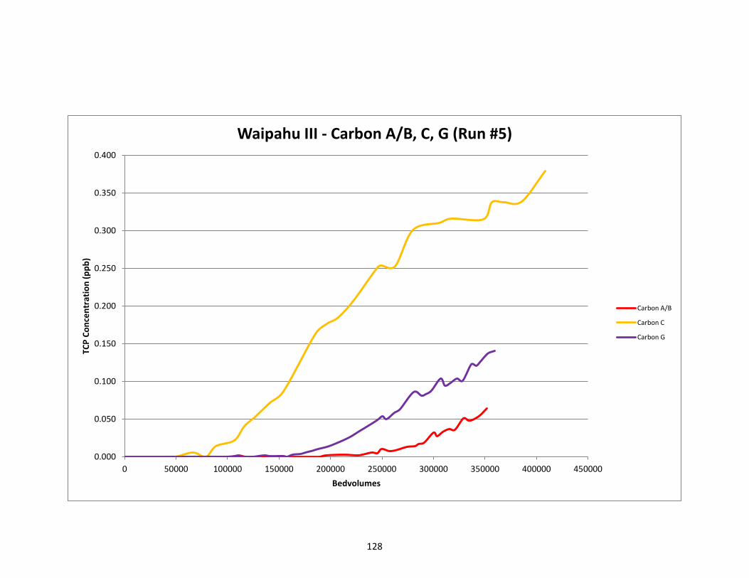
128
0.000
0.050
0.100
0.150
0.200
0.250
0.300
0.350
0.400
0 50000 100000 150000 200000 250000 300000 350000 400000 450000
TCP
Conc
entr
atio
n (p
pb)
Bedvolumes
Waipahu III - Carbon A/B, C, G (Run #5)
Carbon A/B
Carbon C
Carbon G
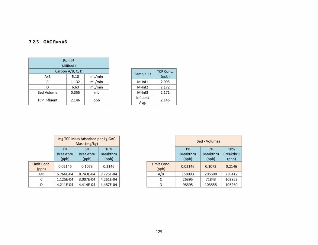
129
7.2.5 GAC Run #6
Run #6 Mililani I
Carbon A/B, C, D Sample ID TCP Conc. (ppb) A/B 5.10 mL/min
C 11.32 mL/min M-Inf1 2.095 D 6.63 mL/min M-Inf2 2.172
Bed Volume 0.355 mL M-Inf3 2.171
TCP Influent 2.146 ppb Influent
Avg. 2.146
mg TCP Mass Adsorbed per kg GAC Mass (mg/kg)
Bed - Volumes
1% Breakthru
(ppb)
5% Breakthru
(ppb)
10% Breakthru
(ppb)
1%
Breakthru (ppb)
5% Breakthru
(ppb)
10% Breakthru
(ppb) Limit Conc.
(ppb) 0.02146 0.1073 0.2146 Limit Conc.
(ppb) 0.02146 0.1073 0.2146
A/B 6.766E-04 8.743E-04 9.725E-04 A/B 158003 205508 230412 C 1.125E-04 3.007E-04 4.261E-04 C 26395 71843 103852 D 4.211E-04 4.414E-04 4.467E-04 D 98395 103555 105260

130
Carbon A/B
Sample ID Date and Time Time between
consecutive samples (min)
Total Time (min)
Total Time (hrs)
Total Time (days)
Flow Rate (mL/min)
Treated Vol. (mL)
Bed Volumes
Conc. (ppb) C/CO
mg TCP Mass Adsorbed per kg GAC Mass
(mg/kg) M-1 5/30/14 23:35 395 395 6.6 0.27 5.49 2169 6109 0.000 0.000 2.62E-05 M-2 5/31/14 8:19 524 919 15.3 0.64 5.49 5045 14212 0.000 0.000 6.10E-05 M-3 5/31/14 14:31 372 1291 21.5 0.90 5.49 7088 19965 0.000 0.000 8.57E-05 M-4 5/31/14 23:49 558 1849 30.8 1.28 5.49 10151 28594 0.000 0.000 1.23E-04 M-6 6/1/14 16:00 971 2820 47.0 1.96 5.11 15113 42571 0.000 0.000 1.83E-04 M-7 6/2/14 0:13 493 3313 55.2 2.30 4.91 17533 49390 0.001 0.000 2.12E-04 M-8 6/2/14 8:25 492 3805 63.4 2.64 4.91 19949 56195 0.001 0.000 2.41E-04 M-9 6/2/14 15:34 429 4234 70.6 2.94 4.91 22056 62128 0.006 0.003 2.67E-04
M-10 6/2/14 23:55 501 4735 78.9 3.29 4.99 24556 69171 0.001 0.000 2.97E-04 M-11 6/3/14 8:37 522 5257 87.6 3.65 4.99 27160 76508 0.004 0.002 3.28E-04 M-12 6/3/14 16:00 443 5700 95.0 3.96 4.99 29371 82735 0.001 0.000 3.55E-04 M-13 6/3/14 23:30 450 6150 102.5 4.27 5.05 31643 89136 0.001 0.000 3.82E-04 M-14 6/4/14 8:23 533 6683 111.4 4.64 5.05 34335 96718 0.003 0.001 4.15E-04 M-15 6/4/14 15:00 397 7080 118.0 4.92 5.05 36340 102366 0.003 0.001 4.39E-04 M-16 6/4/14 23:30 510 7590 126.5 5.27 5.08 38931 109664 0.009 0.004 4.70E-04 M-17 6/5/14 8:40 550 8140 135.7 5.65 5.08 41725 117534 0.006 0.003 5.04E-04 M-18 6/5/14 13:05 265 8405 140.1 5.84 4.99 43047 121259 0.004 0.002 5.20E-04 M-19 6/5/14 21:35 510 8915 148.6 6.19 4.99 45592 128428 0.007 0.003 5.51E-04 M-20 6/6/14 8:40 665 9580 159.7 6.65 5.00 48917 137794 0.010 0.005 5.91E-04 M-21 6/6/14 15:25 405 9985 166.4 6.93 5.00 50942 143498 0.014 0.007 6.15E-04 M-23 6/7/14 8:00 995 10980 183.0 7.63 5.00 55917 157513 0.021 0.010 6.74E-04 M-24 6/7/14 15:34 454 11434 190.6 7.94 5.00 58187 163907 0.027 0.013 7.02E-04 M-25 6/7/14 23:15 461 11895 198.2 8.26 5.00 60492 170400 0.042 0.020 7.29E-04 M-26 6/8/14 9:41 626 12521 208.7 8.70 5.00 63622 179217 0.052 0.024 7.66E-04 M-27 6/8/14 16:02 381 12902 215.0 8.96 5.00 65527 184583 0.062 0.029 7.88E-04 M-28 6/8/14 23:30 448 13350 222.5 9.27 5.00 67767 190893 0.070 0.033 8.14E-04 M-29 6/9/14 8:37 547 13897 231.6 9.65 5.00 70502 198597 0.087 0.041 8.46E-04 M-30 6/9/14 14:39 362 14259 237.7 9.90 5.00 72312 203696 0.101 0.047 8.67E-04 M-31 6/9/14 23:30 531 14790 246.5 10.27 5.00 74967 211175 0.127 0.059 8.97E-04

131
M-32 6/10/14 8:37 547 15337 255.6 10.65 5.00 77702 218879 0.168 0.078 9.28E-04 M-33 6/10/14 14:07 330 15667 261.1 10.88 5.00 79352 223527 0.181 0.084 9.46E-04 M-34 6/10/14 22:07 480 16147 269.1 11.21 5.00 81752 230287 0.214 0.100 9.72E-04 M-35 6/11/14 9:28 681 16828 280.5 11.69 5.00 85157 239879 0.260 0.121 1.01E-03 M-36 6/11/14 15:54 386 17214 286.9 11.95 5.00 87087 245315 0.287 0.134 1.03E-03 M-37 6/12/14 0:05 491 17705 295.1 12.30 5.00 89542 252231 0.326 0.152 1.05E-03 M-38 6/12/14 8:35 510 18215 303.6 12.65 5.00 92092 259414 0.376 0.175 1.08E-03

132
Carbon C
Sample ID Date and Time Time between
consecutive samples (min)
Total Time (min)
Total Time (hrs)
Total Time (days)
Flow Rate (mL/min)
Treated Vol. (mL)
Bed Volumes
Conc. (ppb) C/CO
mg TCP Mass Adsorbed per kg GAC Mass
(mg/kg) M-1 5/30/14 23:35 395 395 6.6 0.27 10.69 4223 11895 0.004 0.002 5.10E-05 M-2 5/31/14 8:19 524 919 15.3 0.64 10.69 9824 27674 0.023 0.011 1.18E-04 M-3 5/31/14 14:31 372 1291 21.5 0.90 10.69 13801 38875 0.038 0.018 1.65E-04 M-4 5/31/14 23:49 558 1849 30.8 1.28 10.69 19766 55678 0.075 0.035 2.35E-04 M-5 6/1/14 7:26 457 2306 38.4 1.60 10.69 24651 69440 0.099 0.046 2.91E-04 M-6 6/1/14 16:00 514 2820 47.0 1.96 10.80 30202 85077 0.153 0.071 3.53E-04 M-7 6/2/14 0:13 493 3313 55.2 2.30 10.32 35290 99409 0.2 0.093 4.09E-04 M-8 6/2/14 8:25 492 3805 63.4 2.64 10.32 40368 113711 0.247 0.115 4.64E-04 M-9 6/2/14 15:34 429 4234 70.6 2.94 10.32 44795 126183 1.103 0.514 4.90E-04
M-10 6/2/14 23:55 501 4735 78.9 3.29 10.50 50055 141001 1.136 0.529 5.19E-04 M-11 6/3/14 8:37 522 5257 87.6 3.65 10.50 55536 156440 1.187 0.553 5.49E-04 M-12 6/3/14 16:00 443 5700 95.0 3.96 10.50 60188 169543 1.326 0.618 5.71E-04 M-13 6/3/14 23:30 450 6150 102.5 4.27 11.84 65516 184552 1.391 0.648 5.93E-04 M-14 6/4/14 8:23 533 6683 111.4 4.64 11.84 71827 202328 1.465 0.683 6.17E-04 M-15 6/4/14 15:00 397 7080 118.0 4.92 11.84 76527 215569 1.535 0.715 6.34E-04 M-16 6/4/14 23:30 510 7590 126.5 5.27 11.33 82305 231846 1.557 0.726 6.53E-04 M-17 6/5/14 8:40 550 8140 135.7 5.65 11.33 88537 249399 1.62 0.755 6.71E-04

133
Carbon D
Sample ID Date and Time Time between
consecutive samples (min)
Total Time (min)
Total Time (hrs)
Total Time (days)
Flow Rate (mL/min)
Treated Vol. (mL)
Bed Volumes
Conc. (ppb) C/CO
mg TCP Mass Adsorbed per kg GAC Mass
(mg/kg) M-1 5/30/14 23:35 395 395 6.6 0.27 5.56 2196 6186 0.000 0.000 2.66E-05 M-2 5/31/14 8:19 524 919 15.3 0.64 5.56 5110 14393 0.000 0.000 6.18E-05 M-3 5/31/14 14:31 372 1291 21.5 0.90 5.56 7178 20220 0.000 0.000 8.68E-05 M-4 5/31/14 23:49 558 1849 30.8 1.28 5.56 10280 28959 0.002 0.001 1.24E-04 M-5 6/1/14 7:26 457 2306 38.4 1.60 5.56 12821 36117 0.001 0.000 1.55E-04 M-7 6/2/14 0:13 1007 3313 55.2 2.30 8.25 21129 59519 0.004 0.002 2.55E-04 M-8 6/2/14 8:25 492 3805 63.4 2.64 8.25 25188 70952 0.006 0.003 3.04E-04 M-9 6/2/14 15:34 429 4234 70.6 2.94 8.25 28727 80922 0.011 0.005 3.47E-04
M-10 6/2/14 23:55 501 4735 78.9 3.29 7.40 32435 91366 0.015 0.007 3.91E-04 M-11 6/3/14 8:37 522 5257 87.6 3.65 7.40 36298 102247 0.025 0.012 4.37E-04 M-12 6/3/14 16:00 443 5700 95.0 3.96 7.40 39576 111481 0.606 0.282 4.66E-04 M-13 6/3/14 23:30 450 6150 102.5 4.27 5.96 42258 119036 0.71 0.331 4.88E-04 M-14 6/4/14 8:23 533 6683 111.4 4.64 5.96 45434 127984 0.755 0.352 5.12E-04 M-15 6/4/14 15:00 397 7080 118.0 4.92 5.96 47801 134649 0.713 0.332 5.32E-04 M-16 6/4/14 23:30 510 7590 126.5 5.27 6.84 51289 144476 0.799 0.372 5.58E-04 M-17 6/5/14 8:40 550 8140 135.7 5.65 6.84 55051 155073 0.872 0.406 5.85E-04

134
0.000
0.200
0.400
0.600
0.800
1.000
1.200
1.400
1.600
1.800
0 50000 100000 150000 200000 250000 300000
TCP
Conc
entr
atio
n (p
pb)
Bedvolumes
Mililani I - Carbon A/B, C, D (Run #6)
Carbon A/B
Carbon C
Carbon D

135
7.2.6 GAC Run #7
Run #7 Mililani I
Carbon E, F, G Sample ID TCP Conc. (ppb) E 6.63 mL/min
F 5.10 mL/min M-Infl1 2.299 G 5.10 mL/min M-Infl2 2.308
Bed Volume 0.355 mL M-Infl3 2.286
TCP Influent 2.298 ppb Influent
Avg. 2.298
mg TCP Mass Adsorbed per kg GAC Mass (mg/kg)
Bed - Volumes
1% Breakthru
(ppb)
5% Breakthru
(ppb)
10% Breakthru
(ppb)
1%
Breakthru (ppb)
5% Breakthru
(ppb)
10% Breakthru
(ppb) Limit Conc.
(ppb) 2.298E-02 1.149E-01 2.298E-01 Limit Conc.
(ppb) 0.0230 0.1149 0.2298
E 4.619E-04 7.026E-04 8.407E-04 E 100757 154737.8 187474.8 F 5.794E-04 7.824E-04 9.279E-04 F 126272 171791 206857.5 G 5.735E-04 7.602E-04 8.730E-04 G 121200 170807.1 197541.8

136
Carbon E
Sample ID Date and Time Time between
consecutive samples (min)
Total Time (min)
Total Time (hrs)
Total Time (days)
Flow Rate (mL/min)
Treated Vol. (mL)
Bed Volumes
Conc. (ppb) C/CO
mg TCP Mass Adsorbed per kg
GAC Mass (mg/kg) M-E1 6/16/14 20:50 395 395 6.6 0.27 7.31 2887 8134 0.002 0.001 3.73E-05 M-E2 6/17/14 8:47 717 1112 18.5 0.77 7.31 8129 22898 0.001 0.000 1.05E-04 M-E3 6/17/14 14:55 368 1480 24.7 1.03 7.31 10819 30475 0 0.000 1.40E-04 M-E4 6/17/14 23:40 525 2005 33.4 1.39 6.56 14263 40177 0 0.000 1.85E-04 M-E5 6/18/14 8:47 547 2552 42.5 1.77 6.56 17851 50285 0.001 0.000 2.31E-04 M-E6 6/18/14 14:52 365 2917 48.6 2.03 6.56 20246 57030 0.002 0.001 2.62E-04 M-E7 6/19/14 0:05 553 3470 57.8 2.41 6.55 23868 67233 0.004 0.002 3.09E-04 M-E8 6/19/14 8:52 527 3997 66.6 2.78 6.55 27320 76956 0.007 0.003 3.53E-04 M-E9 6/19/14 13:51 299 4296 71.6 2.98 6.55 29278 82473 0.01 0.004 3.79E-04
M-E10 6/19/14 23:00 549 4845 80.8 3.36 6.4 32792 92371 0.014 0.006 4.24E-04 M-E11 6/20/14 8:30 570 5415 90.2 3.76 6.4 36440 102647 0.025 0.011 4.70E-04 M-E12 6/20/14 15:36 426 5841 97.4 4.06 6.4 39166 110327 0.031 0.013 5.05E-04 M-E13 6/21/14 0:12 516 6357 105.9 4.41 6.4 42468 119629 0.044 0.019 5.47E-04 M-E14 6/21/14 9:55 583 6940 115.7 4.82 6.4 46200 130140 0.059 0.026 5.94E-04 M-E15 6/21/14 16:19 384 7324 122.1 5.09 6.4 48657 137062 0.076 0.033 6.25E-04 M-E16 6/21/14 23:01 402 7726 128.8 5.37 6.34 51206 144242 0.085 0.037 6.57E-04 M-E17 6/22/14 9:50 649 8375 139.6 5.82 6.34 55321 155832 0.118 0.051 7.07E-04 M-E18 6/22/14 16:00 370 8745 145.7 6.07 6.34 57666 162440 0.142 0.062 7.36E-04 M-E19 6/23/14 0:12 492 9237 153.9 6.41 6.34 60786 171227 0.172 0.075 7.73E-04 M-E20 6/23/14 8:03 471 9708 161.8 6.74 6.34 63772 179639 0.209 0.091 8.08E-04 M-E21 6/23/14 15:13 430 10138 169.0 7.04 6.34 66498 187318 0.229 0.100 8.40E-04 M-E22 6/23/14 23:27 494 10632 177.2 7.38 6.61 69763 196516 0.274 0.119 8.77E-04 M-E23 6/24/14 7:52 505 11137 185.6 7.73 6.61 73101 205919 0.317 0.138 9.15E-04 M-E24 6/24/14 15:00 428 11565 192.8 8.03 6.61 75930 213888 0.369 0.161 9.45E-04 M-E25 6/24/14 22:55 475 12040 200.7 8.36 6.61 79070 222733 0.436 0.190 9.78E-04 M-E26 6/25/14 8:05 550 12590 209.8 8.74 6.61 82706 232974 0.461 0.201 1.02E-03
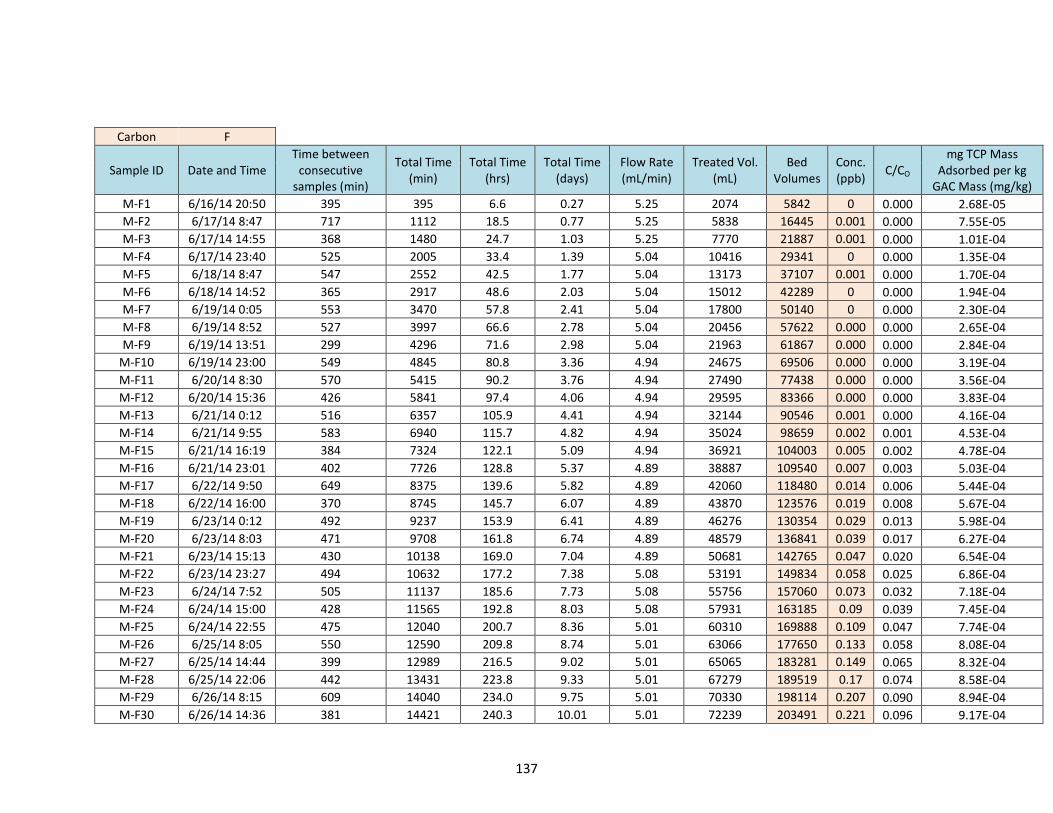
137
Carbon F
Sample ID Date and Time Time between
consecutive samples (min)
Total Time (min)
Total Time (hrs)
Total Time (days)
Flow Rate (mL/min)
Treated Vol. (mL)
Bed Volumes
Conc. (ppb) C/CO
mg TCP Mass Adsorbed per kg
GAC Mass (mg/kg) M-F1 6/16/14 20:50 395 395 6.6 0.27 5.25 2074 5842 0 0.000 2.68E-05 M-F2 6/17/14 8:47 717 1112 18.5 0.77 5.25 5838 16445 0.001 0.000 7.55E-05 M-F3 6/17/14 14:55 368 1480 24.7 1.03 5.25 7770 21887 0.001 0.000 1.01E-04 M-F4 6/17/14 23:40 525 2005 33.4 1.39 5.04 10416 29341 0 0.000 1.35E-04 M-F5 6/18/14 8:47 547 2552 42.5 1.77 5.04 13173 37107 0.001 0.000 1.70E-04 M-F6 6/18/14 14:52 365 2917 48.6 2.03 5.04 15012 42289 0 0.000 1.94E-04 M-F7 6/19/14 0:05 553 3470 57.8 2.41 5.04 17800 50140 0 0.000 2.30E-04 M-F8 6/19/14 8:52 527 3997 66.6 2.78 5.04 20456 57622 0.000 0.000 2.65E-04 M-F9 6/19/14 13:51 299 4296 71.6 2.98 5.04 21963 61867 0.000 0.000 2.84E-04
M-F10 6/19/14 23:00 549 4845 80.8 3.36 4.94 24675 69506 0.000 0.000 3.19E-04 M-F11 6/20/14 8:30 570 5415 90.2 3.76 4.94 27490 77438 0.000 0.000 3.56E-04 M-F12 6/20/14 15:36 426 5841 97.4 4.06 4.94 29595 83366 0.000 0.000 3.83E-04 M-F13 6/21/14 0:12 516 6357 105.9 4.41 4.94 32144 90546 0.001 0.000 4.16E-04 M-F14 6/21/14 9:55 583 6940 115.7 4.82 4.94 35024 98659 0.002 0.001 4.53E-04 M-F15 6/21/14 16:19 384 7324 122.1 5.09 4.94 36921 104003 0.005 0.002 4.78E-04 M-F16 6/21/14 23:01 402 7726 128.8 5.37 4.89 38887 109540 0.007 0.003 5.03E-04 M-F17 6/22/14 9:50 649 8375 139.6 5.82 4.89 42060 118480 0.014 0.006 5.44E-04 M-F18 6/22/14 16:00 370 8745 145.7 6.07 4.89 43870 123576 0.019 0.008 5.67E-04 M-F19 6/23/14 0:12 492 9237 153.9 6.41 4.89 46276 130354 0.029 0.013 5.98E-04 M-F20 6/23/14 8:03 471 9708 161.8 6.74 4.89 48579 136841 0.039 0.017 6.27E-04 M-F21 6/23/14 15:13 430 10138 169.0 7.04 4.89 50681 142765 0.047 0.020 6.54E-04 M-F22 6/23/14 23:27 494 10632 177.2 7.38 5.08 53191 149834 0.058 0.025 6.86E-04 M-F23 6/24/14 7:52 505 11137 185.6 7.73 5.08 55756 157060 0.073 0.032 7.18E-04 M-F24 6/24/14 15:00 428 11565 192.8 8.03 5.08 57931 163185 0.09 0.039 7.45E-04 M-F25 6/24/14 22:55 475 12040 200.7 8.36 5.01 60310 169888 0.109 0.047 7.74E-04 M-F26 6/25/14 8:05 550 12590 209.8 8.74 5.01 63066 177650 0.133 0.058 8.08E-04 M-F27 6/25/14 14:44 399 12989 216.5 9.02 5.01 65065 183281 0.149 0.065 8.32E-04 M-F28 6/25/14 22:06 442 13431 223.8 9.33 5.01 67279 189519 0.17 0.074 8.58E-04 M-F29 6/26/14 8:15 609 14040 234.0 9.75 5.01 70330 198114 0.207 0.090 8.94E-04 M-F30 6/26/14 14:36 381 14421 240.3 10.01 5.01 72239 203491 0.221 0.096 9.17E-04

138
Carbon G
Sample ID Date and Time Time between
consecutive samples (min)
Total Time (min)
Total Time (hrs)
Total Time (days)
Flow Rate (mL/min)
Treated Vol. (mL)
Bed Volumes
Conc. (ppb) C/CO
mg TCP Mass Adsorbed per kg
GAC Mass (mg/kg) M-G1 6/16/14 20:50 395 395 6.6 0.27 5.62 2220 6253 0.002 0.001 2.87E-05 M-G3 6/17/14 14:55 1085 1480 24.7 1.03 5.62 8318 23430 0 0.000 1.08E-04 M-G4 6/17/14 23:40 525 2005 33.4 1.39 4.77 9564 26940 0 0.000 1.40E-04 M-G5 6/18/14 8:47 547 2552 42.5 1.77 4.77 12173 34290 0 0.000 1.74E-04 M-G6 6/18/14 14:52 365 2917 48.6 2.03 4.77 13914 39195 0 0.000 1.96E-04 M-G7 6/19/14 0:05 553 3470 57.8 2.41 5.07 17593 49557 0 0.000 2.33E-04 M-G8 6/19/14 8:52 527 3997 66.6 2.78 5.07 20265 57084 0.000 0.000 2.67E-04 M-G9 6/19/14 13:51 299 4296 71.6 2.98 5.07 21781 61354 0.000 0.000 2.87E-04
M-G10 6/19/14 23:00 549 4845 80.8 3.36 4.88 23644 66602 0.000 0.000 3.22E-04 M-G11 6/20/14 8:30 570 5415 90.2 3.76 4.88 26425 74437 0.000 0.000 3.58E-04 M-G12 6/20/14 15:36 426 5841 97.4 4.06 4.88 28504 80293 0.000 0.000 3.84E-04 M-G13 6/21/14 0:12 516 6357 105.9 4.41 4.88 31022 87386 0.001 0.000 4.17E-04 M-G14 6/21/14 9:55 583 6940 115.7 4.82 4.88 33867 95401 0.004 0.002 4.54E-04 M-G15 6/21/14 16:19 384 7324 122.1 5.09 4.88 35741 100679 0.007 0.003 4.78E-04 M-G16 6/21/14 23:01 402 7726 128.8 5.37 4.86 37548 105770 0.008 0.003 5.03E-04 M-G17 6/22/14 9:50 649 8375 139.6 5.82 4.86 40702 114655 0.017 0.007 5.44E-04 M-G18 6/22/14 16:00 370 8745 145.7 6.07 4.86 42501 119720 0.021 0.009 5.67E-04 M-G19 6/23/14 0:12 492 9237 153.9 6.41 4.86 44892 126456 0.03 0.013 5.97E-04 M-G20 6/23/14 8:03 471 9708 161.8 6.74 4.86 47181 132904 0.044 0.019 6.26E-04 M-G21 6/23/14 15:13 430 10138 169.0 7.04 4.86 49271 138791 0.051 0.022 6.53E-04 M-G22 6/23/14 23:27 494 10632 177.2 7.38 5.13 54542 153640 0.064 0.028 6.85E-04 M-G23 6/24/14 7:52 505 11137 185.6 7.73 5.13 57133 160937 0.083 0.036 7.17E-04 M-G24 6/24/14 15:00 428 11565 192.8 8.03 5.13 59328 167122 0.102 0.044 7.44E-04 M-G25 6/24/14 22:55 475 12040 200.7 8.36 5.13 61765 173986 0.126 0.055 7.74E-04 M-G26 6/25/14 8:05 550 12590 209.8 8.74 5.13 64587 181934 0.164 0.071 8.08E-04 M-G27 6/25/14 14:44 399 12989 216.5 9.02 5.13 66634 187700 0.19 0.083 8.32E-04 M-G28 6/25/14 22:06 442 13431 223.8 9.33 5.13 68901 194087 0.207 0.090 8.59E-04 M-G29 6/26/14 8:15 609 14040 234.0 9.75 5.13 72025 202888 0.265 0.115 8.95E-04 M-G30 6/26/14 14:36 381 14421 240.3 10.01 5.13 73980 208394 0.307 0.134 9.17E-04
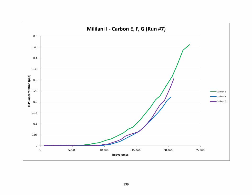
139
0
0.05
0.1
0.15
0.2
0.25
0.3
0.35
0.4
0.45
0.5
0 50000 100000 150000 200000 250000
TCP
Conc
entr
atio
n (p
pb)
Bedvolumes
Mililani I - Carbon E, F, G (Run #7)
Carbon E
Carbon F
Carbon G

140
7.2.7 GAC Run #8
Run #8 Kunia I
Carbon D, F, G Sample ID TCP Conc. (ppb) D 6.63 mL/min
F 5.10 mL/min K-Infl1 0.800 G 5.10 mL/min K-Infl2 0.805
Bed Volume 0.355 mL Influent
Avg. 0.803
TCP Influent 0.803 ppb
mg TCP Mass Adsorbed per kg GAC Mass (mg/kg) Bed - Volumes
1% Breakthru
5% Breakthru
(ppb)
10% Breakthru
1% Breakthru
(ppb)
5% Breakthru
(ppb)
10% Breakthru
(ppb) Limit Conc. (ppb) 0.0080 0.0401 0.0803
Limit Conc. (ppb) 0.0080 0.0401 0.0803
D 2.583E-
04 3.369E-
04 3.818E-04
D 164224 214707 245779
F 1.443E-
04 2.156E-
04 2.533E-04
F 90183 135942 161667
G 8.854E-
05 1.583E-
04 2.328E-04
G 55465 100264 150391

141
Carbon D
Sample ID Date and Time Time between
consecutive samples (min)
Total Time (min)
Total Time (hrs)
Total Time (days)
Flow Rate (mL/min)
Treated Vol. (mL)
Bed Volumes
Conc. (ppb) C/CO
mg TCP Mass Adsorbed per kg
GAC Mass (mg/kg)
M-D1 7/10/14 15:30 90 395 6.6 0.27 3.64 1438 4050 0 0.000 1.48E-06 M-D2 7/10/14 23:20 470 865 14.4 0.60 3.64 3149 8869 0 0.000 9.22E-06 M-D3 7/11/14 8:00 520 1385 23.1 0.96 4.91 5702 16061 0 0.000 2.08E-05 M-D4 7/11/14 15:30 450 1835 30.6 1.27 6.92 8816 24833 0 0.000 3.48E-05 M-D5 7/11/14 23:37 487 2322 38.7 1.61 6.92 12186 34326 0 0.000 5.01E-05 M-D6 7/12/14 8:00 503 2825 47.1 1.96 6.92 15667 44131 0 0.000 6.58E-05 M-D7 7/12/14 16:30 510 3335 55.6 2.32 6.92 19196 54073 0.001 0.001 8.17E-05 M-D8 7/12/14 23:40 430 3765 62.7 2.61 6.92 22171 62455 0 0.000 9.52E-05 M-D9 7/13/14 7:30 470 4235 70.6 2.94 6.92 25424 71616 0 0.000 1.10E-04
M-D10 7/13/14 15:50 500 4735 78.9 3.29 6.92 28884 81363 0 0.000 1.26E-04 M-D11 7/13/14 23:20 450 5185 86.4 3.60 6.92 31998 90135 0 0.000 1.40E-04 M-D12 7/14/14 8:00 520 5705 95.1 3.96 6.92 35596 100271 0.001 0.001 1.56E-04 M-D13 7/14/14 15:45 465 6170 102.8 4.28 6.92 38814 109335 0 0.000 1.70E-04 M-D14 7/14/14 23:47 482 6652 110.9 4.62 6.92 42149 118731 0.001 0.001 1.85E-04 M-D15 7/15/14 8:05 498 7150 119.2 4.97 6.92 45596 128438 0 0.000 2.01E-04 M-D16 7/15/14 15:20 435 7585 126.4 5.27 6.92 48606 136918 0 0.000 2.15E-04 M-D17 7/15/14 23:00 460 8045 134.1 5.59 6.65 51665 145535 0 0.000 2.29E-04 M-D18 7/16/14 8:00 540 8585 143.1 5.96 6.65 55256 155650 0.005 0.006 2.45E-04 M-D19 7/16/14 15:34 454 9039 150.6 6.28 6.65 58275 164155 0.008 0.010 2.58E-04 M-D20 7/16/14 23:00 446 9485 158.1 6.59 6.65 61241 172509 0.011 0.014 2.71E-04 M-D21 7/17/14 8:15 555 10040 167.3 6.97 6.6 64904 182828 0.014 0.017 2.88E-04 M-D22 7/17/14 15:00 405 10445 174.1 7.25 6.6 67577 190357 0.02 0.025 2.99E-04 M-D23 7/17/14 23:48 528 10973 182.9 7.62 6.6 71062 200174 0.028 0.035 3.15E-04 M-D24 7/18/14 8:15 507 11480 191.3 7.97 6.25 74230 209100 0.035 0.044 3.28E-04 M-D25 7/18/14 15:30 435 11915 198.6 8.27 6.25 76949 216758 0.042 0.052 3.40E-04 M-D26 7/18/14 23:50 500 12415 206.9 8.62 6.25 80074 225561 0.055 0.069 3.53E-04 M-D27 7/19/14 7:15 445 12860 214.3 8.93 6.25 82855 233395 0.067 0.083 3.65E-04 M-D32 7/20/14 23:57 2442 15302 255.0 10.63 6.25 98118 276388 0.113 0.141 4.24E-04 M-D33 7/21/14 8:05 488 15790 263.2 10.97 6.25 101168 284980 0.133 0.166 4.35E-04

142
M-D34 7/21/14 16:00 475 16265 271.1 11.30 6.25 104137 293343 0.151 0.188 4.46E-04 M-D35 7/21/14 23:00 420 16685 278.1 11.59 6.25 106762 300737 0.169 0.211 4.56E-04 M-D36 7/22/14 8:29 569 17254 287.6 11.98 6.25 110318 310755 0.199 0.248 4.68E-04 M-D37 7/22/14 14:39 370 17624 293.7 12.24 6.25 112630 317269 0.212 0.264 4.76E-04 M-D38 7/22/14 23:05 506 18130 302.2 12.59 6.25 115793 326177 0.229 0.285 4.86E-04 M-D39 7/23/14 8:09 544 18674 311.2 12.97 6.25 119193 335755 0.249 0.310 4.96E-04

143
Carbon F
Sample ID Date and Time Time between
consecutive samples (min)
Total Time (min)
Total Time (hrs)
Total Time (days)
Flow Rate (mL/min)
Treated Vol. (mL)
Bed Volumes
Conc. (ppb) C/CO
mg TCP Mass Adsorbed per kg
GAC Mass (mg/kg)
M-F9 7/13/14 7:30 810 810 13.5 0.56 5.19 4204 11842 0.000 0.000 1.90E-05 M-F10 7/13/14 15:50 500 1310 21.8 0.91 5.19 6799 19152 0.000 0.000 3.07E-05 M-F11 7/13/14 23:20 450 1760 29.3 1.22 5.19 9134 25731 0.000 0.000 4.13E-05 M-F12 7/14/14 8:00 520 2280 38.0 1.58 5.19 11833 33333 0.002 0.002 5.35E-05 M-F13 7/14/14 15:45 465 2745 45.8 1.91 5.19 14247 40131 0.000 0.000 6.44E-05 M-F14 7/14/14 23:47 482 3227 53.8 2.24 5.19 16748 47178 0.002 0.002 7.57E-05 M-F15 7/15/14 8:05 498 3725 62.1 2.59 5.19 19333 54458 0.001 0.001 8.73E-05 M-F16 7/15/14 15:20 435 4160 69.3 2.89 5.19 21590 60818 0.000 0.000 9.75E-05 M-F17 7/15/14 23:00 460 4620 77.0 3.21 5.18 23973 67530 0.003 0.004 1.08E-04 M-F19 7/16/14 15:34 994 5614 93.6 3.90 5.18 29122 82034 0.006 0.007 1.31E-04 M-F20 7/16/14 23:00 446 6060 101.0 4.21 5.18 31432 88542 0.007 0.009 1.42E-04 M-F21 7/17/14 8:15 555 6615 110.3 4.59 5.12 34274 96546 0.012 0.015 1.54E-04 M-F22 7/17/14 15:00 405 7020 117.0 4.88 5.12 36348 102388 0.013 0.016 1.64E-04 M-F23 7/17/14 23:48 528 7548 125.8 5.24 5.12 39051 110003 0.017 0.021 1.76E-04 M-F24 7/18/14 8:15 507 8055 134.3 5.59 4.56 41363 116515 0.020 0.025 1.86E-04 M-F25 7/18/14 15:30 435 8490 141.5 5.90 4.56 43346 122103 0.026 0.032 1.94E-04 M-F26 7/18/14 23:50 500 8990 149.8 6.24 4.56 45626 128525 0.031 0.039 2.04E-04 M-F27 7/19/14 7:15 445 9435 157.3 6.55 4.56 47656 134241 0.038 0.047 2.13E-04 M-F30 7/20/14 8:10 1495 10930 182.2 7.59 4.56 54473 153445 0.062 0.077 2.42E-04 M-F32 7/20/14 23:57 947 11877 198.0 8.25 4.56 58791 165609 0.089 0.111 2.59E-04 M-F33 7/21/14 8:05 488 12365 206.1 8.59 4.56 61016 171877 0.165 0.206 2.67E-04 M-F34 7/21/14 16:00 475 12840 214.0 8.92 4.56 63182 177979 0.156 0.194 2.75E-04 M-F35 7/21/14 23:00 420 13260 221.0 9.21 4.56 65098 183374 0.159 0.198 2.82E-04 M-F36 7/22/14 8:29 569 13829 230.5 9.60 4.56 67692 190683 0.170 0.212 2.91E-04 M-F37 7/22/14 14:39 370 14199 236.7 9.86 4.56 69380 195435 0.169 0.211 2.97E-04 M-F38 7/22/14 23:05 506 14705 245.1 10.21 4.56 71687 201935 0.172 0.214 3.05E-04 M-F39 7/23/14 8:09 544 15249 254.2 10.59 4.56 74168 208923 0.175 0.218 3.14E-04

144
Carbon G
Sample ID Date and Time Time between
consecutive samples (min)
Total Time (min)
Total Time (hrs)
Total Time (days)
Flow Rate (mL/min)
Treated Vol. (mL)
Bed Volumes
Conc. (ppb) C/CO
mg TCP Mass Adsorbed per kg
GAC Mass (mg/kg)
M-G1 7/10/14 15:30 395 395 6.6 0.27 4.79 1892 5330 0.001 0.001 8.54E-06 M-G2 7/10/14 23:20 470 865 14.4 0.60 4.79 4143 11671 0.003 0.004 1.87E-05 M-G3 7/11/14 8:00 520 1385 23.1 0.96 5.6 7055 19874 0.002 0.002 3.18E-05 M-G4 7/11/14 15:30 450 1835 30.6 1.27 5.3 9440 26593 0.003 0.004 4.26E-05 M-G5 7/11/14 23:37 487 2322 38.7 1.61 5.3 12021 33863 0.003 0.004 5.42E-05 M-G6 7/12/14 8:00 503 2825 47.1 1.96 5.3 14687 41373 0.005 0.006 6.62E-05 M-G7 7/12/14 16:30 510 3335 55.6 2.32 5.3 17390 48987 0.009 0.011 7.82E-05 M-G8 7/12/14 23:40 430 3765 62.7 2.61 5.3 19669 55407 0.008 0.010 8.84E-05 M-G9 7/13/14 7:30 470 4235 70.6 2.94 5.3 22160 62424 0.011 0.014 9.96E-05
M-G10 7/13/14 15:50 500 4735 78.9 3.29 5.3 24810 69888 0.012 0.015 1.11E-04 M-G11 7/13/14 23:20 450 5185 86.4 3.60 5.3 27195 76607 0.014 0.017 1.22E-04 M-G12 7/14/14 8:00 520 5705 95.1 3.96 5.3 29951 84370 0.023 0.029 1.34E-04 M-G13 7/14/14 15:45 465 6170 102.8 4.28 5.3 32416 91312 0.037 0.046 1.45E-04 M-G14 7/14/14 23:47 482 6652 110.9 4.62 5.3 34970 98508 0.038 0.047 1.56E-04 M-G15 7/15/14 8:05 498 7150 119.2 4.97 5.3 37610 105943 0.047 0.059 1.67E-04 M-G16 7/15/14 15:20 435 7585 126.4 5.27 5.3 39915 112438 0.046 0.057 1.77E-04 M-G17 7/15/14 23:00 460 8045 134.1 5.59 5.22 42317 119202 0.046 0.057 1.87E-04 M-G18 7/16/14 8:00 540 8585 143.1 5.96 5.22 45135 127142 0.054 0.067 1.99E-04 M-G19 7/16/14 15:34 454 9039 150.6 6.28 5.22 47505 133818 0.063 0.079 2.09E-04 M-G20 7/16/14 23:00 446 9485 158.1 6.59 5.22 49833 140376 0.071 0.088 2.18E-04 M-G21 7/17/14 8:15 555 10040 167.3 6.97 5.07 52647 148302 0.077 0.096 2.30E-04 M-G22 7/17/14 15:00 405 10445 174.1 7.25 5.07 54701 154086 0.086 0.107 2.38E-04 M-G23 7/17/14 23:48 528 10973 182.9 7.62 5.07 57378 161627 0.097 0.121 2.49E-04 M-G24 7/18/14 8:15 507 11480 191.3 7.97 5.07 59948 168868 0.106 0.132 2.59E-04 M-G25 7/18/14 15:30 435 11915 198.6 8.27 5.07 62153 175080 0.105 0.131 2.68E-04 M-G26 7/18/14 23:50 500 12415 206.9 8.62 5.07 64688 182221 0.121 0.151 2.77E-04 M-G27 7/19/14 7:15 445 12860 214.3 8.93 5.07 66945 188576 0.129 0.161 2.86E-04 M-G30 7/20/14 8:10 1495 14355 239.3 9.97 5.07 74524 209927 0.155 0.193 3.13E-04 M-G32 7/20/14 23:57 947 15302 255.0 10.63 5.07 79326 223452 0.190 0.237 3.30E-04 M-G34 7/21/14 16:00 963 16265 271.1 11.30 5.07 84208 237205 0.225 0.280 3.46E-04
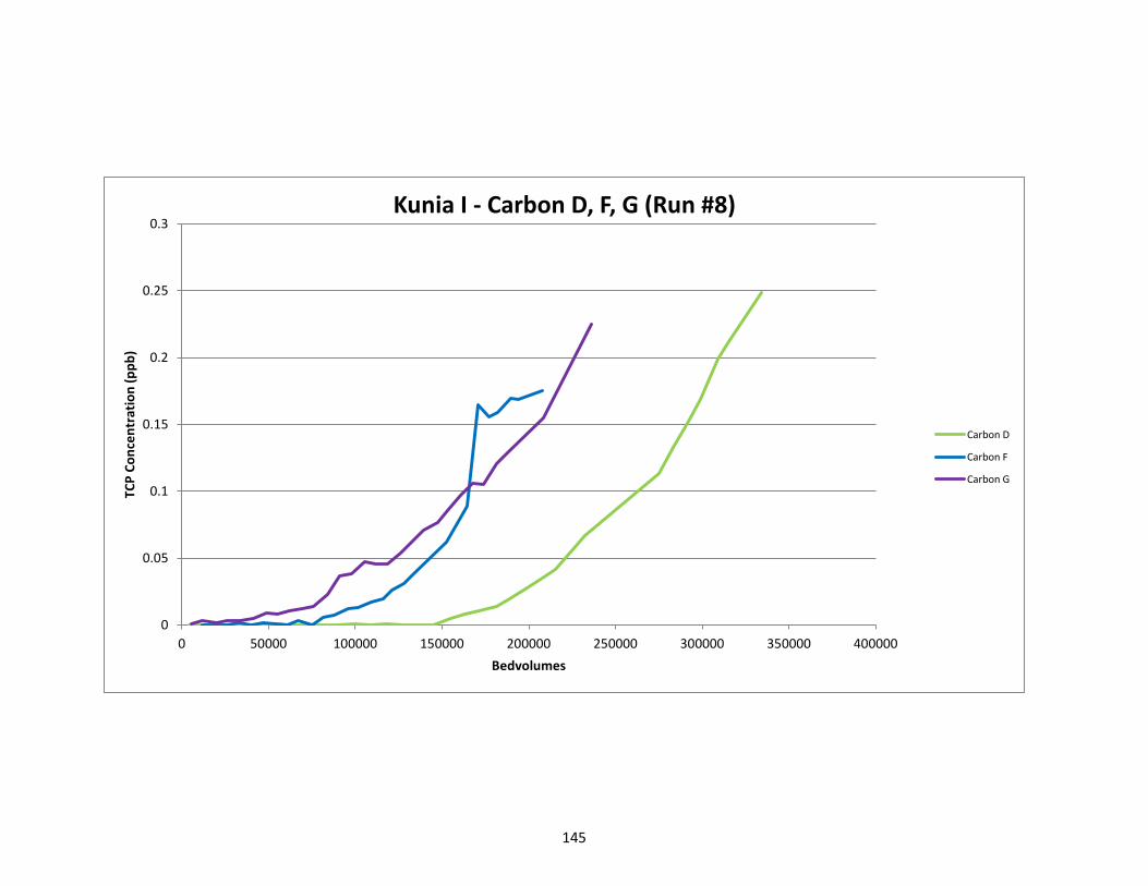
145
0
0.05
0.1
0.15
0.2
0.25
0.3
0 50000 100000 150000 200000 250000 300000 350000 400000
TCP
Conc
entr
atio
n (p
pb)
Bedvolumes
Kunia I - Carbon D, F, G (Run #8)
Carbon D
Carbon F
Carbon G
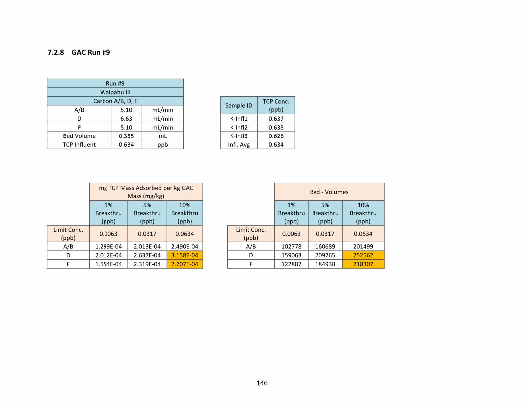
146
7.2.8 GAC Run #9
Run #9 Waipahu III
Carbon A/B, D, F Sample ID TCP Conc. (ppb) A/B 5.10 mL/min
D 6.63 mL/min K-Infl1 0.637 F 5.10 mL/min K-Infl2 0.638
Bed Volume 0.355 mL K-Infl3 0.626 TCP Influent 0.634 ppb Infl. Avg 0.634
mg TCP Mass Adsorbed per kg GAC Mass (mg/kg)
Bed - Volumes
1% Breakthru
(ppb)
5% Breakthru
(ppb)
10% Breakthru
(ppb)
1%
Breakthru (ppb)
5% Breakthru
(ppb)
10% Breakthru
(ppb) Limit Conc.
(ppb) 0.0063 0.0317 0.0634 Limit Conc.
(ppb) 0.0063 0.0317 0.0634
A/B 1.299E-04 2.013E-04 2.490E-04 A/B 102778 160689 201499 D 2.012E-04 2.637E-04 3.158E-04 D 159063 209765 252562 F 1.554E-04 2.319E-04 2.707E-04 F 122887 184938 218307

147
Carbon A/B
Sample ID Date and Time Time between
consecutive samples (min)
Total Time (min)
Total Time (hrs)
Total Time (days)
Flow Rate (mL/min)
Treated Vol. (mL)
Bed Volumes
Conc. (ppb) C/CO
mg TCP Mass Adsorbed per kg GAC Mass
(mg/kg) W-A/B1 7/28/14 14:00 0 0 0.0 0.00 5.13 0 0 0.001 0.002 0 W-A/B2 7/28/14 22:50 530 530 8.8 0.37 5.13 2719 7659 0.002 0.003 9.68E-06 W-A/B3 7/29/14 8:00 550 1080 18.0 0.75 5.13 5540 15607 0.000 0.000 1.97E-05 W-A/B4 7/29/14 15:42 462 1542 25.7 1.07 5.13 7910 22283 0.000 0.000 2.82E-05 W-A/B5 7/30/14 0:00 498 2040 34.0 1.42 5.08 10440 29409 0.000 0.000 3.72E-05 W-A/B6 7/30/14 7:40 460 2500 41.7 1.74 5.07 12772 35979 0.000 0.000 4.56E-05 W-A/B7 7/30/14 15:25 465 2965 49.4 2.06 5.07 15130 42620 0.000 0.000 5.40E-05 W-A/B8 7/30/14 22:00 395 3360 56.0 2.33 5.01 17109 48194 0.000 0.000 6.10E-05 W-A/B9 7/31/14 8:09 609 3969 66.1 2.76 5.01 20160 56789 0.000 0.000 7.19E-05
W-A/B10 7/31/14 15:56 467 4436 73.9 3.08 5.01 22500 63380 0.000 0.000 8.03E-05 W-A/B11 7/31/14 22:25 389 4825 80.4 3.35 5.03 24456 68891 0.001 0.002 8.73E-05 W-A/B12 8/1/14 8:05 580 5405 90.1 3.75 5.03 27374 77109 0.001 0.002 9.77E-05 W-A/B13 8/1/14 14:13 368 5773 96.2 4.01 5.03 29225 82324 0.004 0.006 1.04E-04 W-A/B14 8/1/14 22:00 467 6240 104.0 4.33 5.00 31560 88901 0.003 0.005 1.13E-04 W-A/B15 8/2/14 11:14 794 7034 117.2 4.88 5.00 35530 100084 0.006 0.009 1.27E-04 W-A/B16 8/2/14 13:00 106 7140 119.0 4.96 5.19 36080 101634 0.006 0.009 1.29E-04 W-A/B17 8/2/14 20:45 465 7605 126.8 5.28 5.19 38493 108432 0.008 0.013 1.37E-04 W-A/B18 8/3/14 8:45 720 8325 138.8 5.78 5.19 42230 118958 0.011 0.017 1.50E-04 W-A/B19 8/3/14 15:38 413 8738 145.6 6.07 5.19 44374 124996 0.011 0.017 1.58E-04 W-A/B20 8/3/14 22:19 401 9139 152.3 6.35 5.00 46379 130644 0.017 0.027 1.65E-04 W-A/B21 8/4/14 5:38 439 9578 159.6 6.65 5.00 48574 136827 0.015 0.024 1.72E-04 W-A/B22 8/4/14 15:37 599 10177 169.6 7.07 5.00 51569 145264 0.021 0.033 1.83E-04 W-A/B23 8/4/14 23:14 457 10634 177.2 7.38 5.00 53854 151700 0.024 0.038 1.90E-04 W-A/B24 8/5/14 8:05 531 11165 186.1 7.75 4.98 56498 159149 0.031 0.049 1.99E-04 W-A/B25 8/5/14 16:07 482 11647 194.1 8.09 4.98 58898 165911 0.034 0.054 2.08E-04 W-A/B26 8/6/14 0:05 478 12125 202.1 8.42 4.98 61279 172616 0.037 0.058 2.16E-04 W-A/B27 8/6/14 8:01 476 12601 210.0 8.75 4.98 63649 179294 0.043 0.068 2.23E-04 W-A/B28 8/6/14 13:49 348 12949 215.8 8.99 4.90 65354 184097 0.052 0.082 2.29E-04 W-A/B29 8/6/14 23:10 561 13510 225.2 9.38 4.90 68103 191841 0.054 0.085 2.38E-04 W-A/B30 8/7/14 8:03 533 14043 234.0 9.75 4.90 70715 199197 0.062 0.098 2.46E-04 W-A/B31 8/7/14 14:09 366 14409 240.1 10.01 4.90 72508 204249 0.065 0.103 2.52E-04

148
Carbon D
Sample ID Date and Time Time between
consecutive samples (min)
Total Time (min)
Total Time (hrs)
Total Time (days)
Flow Rate (mL/min)
Treated Vol. (mL)
Bed Volumes
Conc. (ppb) C/CO
mg TCP Mass Adsorbed per kg GAC Mass
(mg/kg) W-D1 7/28/14 14:00 0 0 0.0 0.00 7.12 0 0 0.001 0.002 0 W-D2 7/28/14 22:50 530 530 8.8 0.37 7.12 3774 10630 0.000 0.000 1.35E-05 W-D3 7/29/14 8:00 550 1080 18.0 0.75 7.12 7690 21661 0.002 0.003 2.74E-05 W-D4 7/29/14 15:42 462 1542 25.7 1.07 7.12 10979 30927 0.000 0.000 3.92E-05 W-D5 7/30/14 0:00 498 2040 34.0 1.42 6.3 14116 39765 0.000 0.000 5.04E-05 W-D6 7/30/14 7:40 460 2500 41.7 1.74 6.71 17203 48459 0.000 0.000 6.14E-05 W-D7 7/30/14 15:25 465 2965 49.4 2.06 6.71 20323 57248 0.000 0.000 7.25E-05 W-D8 7/30/14 22:00 395 3360 56.0 2.33 6.58 22922 64570 0.001 0.002 8.18E-05 W-D9 7/31/14 8:09 609 3969 66.1 2.76 6.58 26930 75858 0.000 0.000 9.61E-05
W-D10 7/31/14 15:56 467 4436 73.9 3.08 6.58 30002 84514 0.000 0.000 1.07E-04 W-D11 7/31/14 22:25 389 4825 80.4 3.35 6.47 32519 91603 0.000 0.000 1.16E-04 W-D12 8/1/14 8:05 580 5405 90.1 3.75 6.47 36272 102174 0.000 0.000 1.29E-04 W-D13 8/1/14 14:13 368 5773 96.2 4.01 6.47 38653 108881 0.000 0.000 1.38E-04 W-D14 8/1/14 22:00 467 6240 104.0 4.33 6.62 41744 117590 0.002 0.003 1.49E-04 W-D15 8/2/14 11:14 794 7034 117.2 4.88 6.62 47001 132396 0.002 0.003 1.68E-04 W-D16 8/2/14 13:00 106 7140 119.0 4.96 6.62 47702 134373 0.002 0.003 1.70E-04 W-D17 8/2/14 20:45 465 7605 126.8 5.28 6.62 50781 143044 0.003 0.005 1.81E-04 W-D18 8/3/14 8:45 720 8325 138.8 5.78 6.62 55547 156470 0.006 0.009 1.98E-04 W-D19 8/3/14 15:38 413 8738 145.6 6.07 6.62 58281 164172 0.007 0.011 2.08E-04 W-D20 8/3/14 22:19 401 9139 152.3 6.35 6.15 60747 171119 0.007 0.011 2.16E-04 W-D21 8/4/14 5:38 439 9578 159.6 6.65 6.15 63447 178724 0.009 0.014 2.26E-04 W-D22 8/4/14 15:37 599 10177 169.6 7.07 6.15 67131 189101 0.016 0.025 2.39E-04 W-D23 8/4/14 23:14 457 10634 177.2 7.38 6.15 69941 197018 0.020 0.032 2.48E-04 W-D24 8/5/14 8:05 531 11165 186.1 7.75 6.01 73133 206008 0.028 0.044 2.59E-04 W-D25 8/5/14 16:07 482 11647 194.1 8.09 6.01 76030 214168 0.036 0.057 2.69E-04 W-D26 8/6/14 0:05 478 12125 202.1 8.42 6.01 78902 222260 0.041 0.065 2.79E-04 W-D27 8/6/14 8:01 476 12601 210.0 8.75 6.01 81763 230319 0.046 0.073 2.88E-04

149
Carbon F
Sample ID Date and Time Time between
consecutive samples (min)
Total Time (min)
Total Time (hrs)
Total Time (days)
Flow Rate (mL/min)
Treated Vol. (mL)
Bed Volumes
Conc. (ppb) C/CO
mg TCP Mass Adsorbed per kg GAC Mass
(mg/kg) W-F1 7/28/14 14:00 0 0 0.0 0.00 5.82 0 0 0.000 0.000 0 W-F2 7/28/14 22:50 530 530 8.8 0.37 5.82 3085 8689 0.000 0.000 1.10E-05 W-F3 7/29/14 8:00 550 1080 18.0 0.75 5.82 6286 17706 0.000 0.000 2.24E-05 W-F4 7/29/14 15:42 462 1542 25.7 1.07 5.82 8974 25280 0.000 0.000 3.20E-05 W-F5 7/30/14 0:00 498 2040 34.0 1.42 4.6 11265 31733 0.000 0.000 4.02E-05 W-F6 7/30/14 7:40 460 2500 41.7 1.74 5.04 13584 38264 0.000 0.000 4.85E-05 W-F7 7/30/14 15:25 465 2965 49.4 2.06 5.04 15927 44865 0.000 0.000 5.69E-05 W-F8 7/30/14 22:00 395 3360 56.0 2.33 4.98 17894 50407 0.000 0.000 6.39E-05 W-F9 7/31/14 8:09 609 3969 66.1 2.76 4.98 20927 58950 0.001 0.002 7.47E-05
W-F10 7/31/14 15:56 467 4436 73.9 3.08 4.98 23253 65501 0.000 0.000 8.30E-05 W-F11 7/31/14 22:25 389 4825 80.4 3.35 4.98 25190 70958 0.000 0.000 8.99E-05 W-F12 8/1/14 8:05 580 5405 90.1 3.75 4.98 28078 79094 0.000 0.000 1.00E-04 W-F13 8/1/14 14:13 368 5773 96.2 4.01 4.98 29911 84257 0.000 0.000 1.07E-04 W-F14 8/1/14 22:00 467 6240 104.0 4.33 5.26 32367 91176 0.002 0.003 1.16E-04 W-F15 8/2/14 11:14 794 7034 117.2 4.88 5.26 36544 102941 0.003 0.005 1.30E-04 W-F16 8/2/14 13:00 106 7140 119.0 4.96 5.26 37101 104511 0.002 0.003 1.32E-04 W-F17 8/2/14 20:45 465 7605 126.8 5.28 5.26 39547 111401 0.004 0.006 1.41E-04 W-F18 8/3/14 8:45 720 8325 138.8 5.78 5.26 43335 122069 0.005 0.008 1.54E-04 W-F19 8/3/14 15:38 413 8738 145.6 6.07 5.26 45507 128189 0.015 0.024 1.62E-04 W-F20 8/3/14 22:19 401 9139 152.3 6.35 5.11 47556 133961 0.007 0.011 1.69E-04 W-F21 8/4/14 5:38 439 9578 159.6 6.65 5.11 49799 140280 0.015 0.024 1.77E-04 W-F22 8/4/14 15:37 599 10177 169.6 7.07 5.11 52860 148902 0.012 0.019 1.88E-04 W-F23 8/4/14 23:14 457 10634 177.2 7.38 5.11 55196 155480 0.014 0.022 1.96E-04 W-F24 8/5/14 8:05 531 11165 186.1 7.75 4.98 57840 162929 0.017 0.027 2.05E-04 W-F25 8/5/14 16:07 482 11647 194.1 8.09 4.98 60240 169691 0.021 0.033 2.13E-04 W-F26 8/6/14 0:05 478 12125 202.1 8.42 4.98 62621 176396 0.024 0.038 2.22E-04 W-F27 8/6/14 8:01 476 12601 210.0 8.75 4.98 64991 183074 0.029 0.046 2.30E-04

150
W-F28 8/6/14 13:49 348 12949 215.8 8.99 4.96 66717 187936 0.036 0.057 2.35E-04 W-F29 8/6/14 23:10 561 13510 225.2 9.38 4.96 69500 195774 0.039 0.062 2.45E-04 W-F30 8/7/14 8:03 533 14043 234.0 9.75 4.96 72144 203221 0.043 0.068 2.54E-04 W-F31 8/7/14 14:09 366 14409 240.1 10.01 4.96 73959 208335 0.054 0.085 2.60E-04

151
0.000
0.010
0.020
0.030
0.040
0.050
0.060
0.070
0 50000 100000 150000 200000 250000
TCP
Conc
entr
atio
n (p
pb)
Bedvolumes
Waipahu III - Carbon A/B, D, F (Run #9)
Carbon A/B
Carbon D
Carbon F

152
7.2.9 GAC Run #10
Run #10 Waipahu III
Carbon C, E, G Sample ID TCP Conc. (ppb) C 11.32 mL/min
E 6.63 mL/min K-Infl1 0.637 G 5.10 mL/min K-Infl2 0.638
Bed Volume 0.355 mL K-Infl3 0.626 TCP Influent 0.634 ppb Infl. Avg 0.634
mg TCP Mass Adsorbed per kg GAC Mass (mg/kg)
Bed - Volumes
1% Breakthru
(ppb)
5% Breakthru
(ppb)
10% Breakthru
(ppb)
1%
Breakthru (ppb)
5% Breakthru
(ppb)
10% Breakthru
(ppb) Limit Conc.
(ppb) 0.0063 0.0317 0.0634 Limit Conc.
(ppb) 0.0063 0.0317 0.0634
C 4.438E-05 8.401E-05 1.117E-04 C 35212 67711 91732 E 2.078E-04 2.885E-04 3.410E-04 E 164259 230054 275083 G 1.523E-04 2.316E-04 2.818E-04 G 120380 185023 227708

153
Carbon C
Sample ID Date and Time Time between
consecutive samples (min)
Total Time (min)
Total Time (hrs)
Total Time (days)
Flow Rate (mL/min)
Treated Vol. (mL)
Bed Volumes
Conc. (ppb) C/CO
mg TCP Mass Adsorbed per kg
GAC Mass (mg/kg)
W-C1 8/12/14 16:40 0 0 0.0 0.00 11.18 0 0 0 0.000 0 W-C2 8/12/14 23:17 397 397 6.6 0.28 11.18 4438 12503 0 0.000 1.58E-05 W-C3 8/13/14 8:05 528 925 15.4 0.64 10.92 10204 28744 0.004 0.006 3.63E-05 W-C4 8/13/14 15:28 443 1368 22.8 0.95 11.09 15117 42583 0.009 0.014 5.36E-05 W-C5 8/13/14 23:31 483 1851 30.8 1.29 11.09 20474 57672 0.022 0.035 7.20E-05 W-C6 8/14/14 8:22 531 2382 39.7 1.65 11.09 26362 74260 0.038 0.060 9.18E-05 W-C7 8/14/14 13:30 308 2690 44.8 1.87 10.58 29621 83439 0.047 0.074 1.03E-04 W-C8 8/14/14 23:25 595 3285 54.8 2.28 10.58 35916 101172 0.082 0.129 1.22E-04 W-C9 8/15/14 8:02 517 3802 63.4 2.64 10.58 41386 116580 0.085 0.134 1.39E-04
W-C10 8/15/14 15:15 433 4235 70.6 2.94 10.58 45967 129485 0.102 0.161 1.53E-04 W-C11 8/15/14 23:00 465 4700 78.3 3.26 10.58 50887 143343 0.116 0.183 1.67E-04 W-C12 8/16/14 8:42 582 5282 88.0 3.67 10.58 57044 160688 0.137 0.216 1.84E-04 W-C13 8/16/14 15:01 379 5661 94.4 3.93 10.80 61138 172218 0.159 0.251 1.95E-04 W-C14 8/16/14 23:00 479 6140 102.3 4.26 10.80 66311 186791 0.184 0.290 2.08E-04 W-C15 8/17/14 9:30 630 6770 112.8 4.70 10.80 73115 205957 0.227 0.358 2.24E-04 W-C16 8/17/14 17:00 450 7220 120.3 5.01 10.80 77975 219647 0.244 0.385 2.35E-04 W-C17 8/17/14 23:28 388 7608 126.8 5.28 10.80 82165 231451 0.249 0.393 2.44E-04 W-C18 8/18/14 8:33 545 8153 135.9 5.66 10.80 88051 248031 0.297 0.469 2.55E-04 W-C19 8/18/14 13:49 316 8469 141.1 5.88 11.20 91590 258001 0.301 0.475 2.62E-04 W-C20 8/18/14 21:00 431 8900 148.3 6.18 11.20 96418 271599 0.319 0.503 2.70E-04 W-C21 8/19/14 9:09 729 9629 160.5 6.69 11.20 104582 294598 0.340 0.537 2.84E-04

154
Carbon E
Sample ID Date and Time Time between
consecutive samples (min)
Total Time (min)
Total Time (hrs)
Total Time (days)
Flow Rate (mL/min)
Treated Vol. (mL)
Bed Volumes
Conc. (ppb) C/CO
mg TCP Mass Adsorbed per kg
GAC Mass (mg/kg)
W-E1 8/12/14 16:40 0 0 0.0 0.00 6.62 0 0 0.000 0.000 0 W-E2 8/12/14 23:17 397 397 6.6 0.28 6.72 2668 7515 0.000 0.000 9.52E-06 W-E3 8/13/14 8:05 528 925 15.4 0.64 6.47 6084 17138 0.000 0.000 2.17E-05 W-E4 8/13/14 15:28 443 1368 22.8 0.95 6.64 9026 25424 0.000 0.000 3.22E-05 W-E5 8/13/14 23:31 483 1851 30.8 1.29 6.53 12180 34308 0.000 0.000 4.35E-05 W-E6 8/14/14 8:22 531 2382 39.7 1.65 6.53 15647 44076 0.000 0.000 5.59E-05 W-E7 8/14/14 13:30 308 2690 44.8 1.87 6.08 17520 49351 0.000 0.000 6.25E-05 W-E8 8/14/14 23:25 595 3285 54.8 2.28 6.08 21137 59541 0.000 0.000 7.55E-05 W-E9 8/15/14 8:02 517 3802 63.4 2.64 6.08 24281 68396 0.000 0.000 8.67E-05
W-E10 8/15/14 15:15 433 4235 70.6 2.94 6.08 26913 75812 0.000 0.000 9.61E-05 W-E11 8/15/14 23:00 465 4700 78.3 3.26 6.08 29740 83776 0.000 0.000 1.06E-04 W-E12 8/16/14 8:42 582 5282 88.0 3.67 6.08 33279 93743 0.000 0.000 1.19E-04 W-E13 8/16/14 15:01 379 5661 94.4 3.93 6.50 35742 100683 0.001 0.002 1.28E-04 W-E14 8/16/14 23:00 479 6140 102.3 4.26 6.50 38856 109453 0.000 0.000 1.39E-04 W-E15 8/17/14 9:30 630 6770 112.8 4.70 6.50 42951 120989 0.001 0.002 1.53E-04 W-E16 8/17/14 17:00 450 7220 120.3 5.01 6.50 45876 129228 0.002 0.003 1.64E-04 W-E18 8/18/14 8:33 933 8153 135.9 5.66 6.48 51922 146259 0.004 0.006 1.85E-04 W-E19 8/18/14 13:49 316 8469 141.1 5.88 6.50 53976 152044 0.004 0.006 1.92E-04 W-E20 8/18/14 21:00 431 8900 148.3 6.18 6.50 56777 159936 0.005 0.008 2.02E-04 W-E21 8/19/14 9:09 729 9629 160.5 6.69 6.30 61370 172873 0.009 0.014 2.19E-04 W-E22 8/19/14 17:03 474 10103 168.4 7.02 6.30 64356 181285 0.012 0.019 2.29E-04 W-E23 8/19/14 23:23 380 10483 174.7 7.28 6.30 66750 188029 0.014 0.022 2.37E-04 W-E24 8/20/14 9:01 578 11061 184.4 7.68 6.30 70392 198286 0.019 0.030 2.50E-04 W-E25 8/20/14 14:42 341 11402 190.0 7.92 6.30 72540 204338 0.020 0.032 2.57E-04 W-E26 8/20/14 23:44 542 11944 199.1 8.29 6.30 75954 213956 0.025 0.039 2.69E-04 W-E27 8/21/14 7:55 491 12435 207.2 8.64 6.30 79048 222670 0.028 0.044 2.80E-04 W-E28 8/21/14 15:05 430 12865 214.4 8.93 6.62 81894 230688 0.032 0.050 2.89E-04 W-E29 8/21/14 22:40 455 13320 222.0 9.25 6.62 84906 239173 0.038 0.060 2.99E-04 W-E30 8/22/14 8:52 612 13932 232.2 9.67 6.62 88958 250586 0.047 0.074 3.13E-04 W-E31 8/22/14 15:30 398 14330 238.8 9.95 6.62 91593 258008 0.048 0.076 3.21E-04 W-E32 8/23/14 0:51 561 14891 248.2 10.34 6.69 95346 268580 0.060 0.095 3.34E-04

155
W-E33 8/23/14 7:41 410 15301 255.0 10.63 6.69 98089 276306 0.064 0.101 3.42E-04 W-E34 8/23/14 13:52 371 15672 261.2 10.88 6.69 100571 283298 0.071 0.112 3.50E-04 W-E35 8/23/14 21:50 478 16150 269.2 11.22 6.69 103768 292306 0.075 0.118 3.60E-04 W-E36 8/24/14 11:07 797 16947 282.4 11.77 6.69 109100 307325 0.086 0.136 3.77E-04 W-E37 8/24/14 14:27 200 17147 285.8 11.91 6.69 110438 311094 0.086 0.136 3.81E-04 W-E38 8/25/14 4:45 858 18005 300.1 12.50 6.69 116178 327263 0.105 0.166 3.98E-04 W-E40 8/25/14 14:24 579 18584 309.7 12.91 6.71 120064 338207 0.108 0.170 4.10E-04 W-E41 8/25/14 21:30 426 19010 316.8 13.20 6.71 122922 346259 0.110 0.174 4.18E-04 W-E42 8/26/14 9:00 690 19700 328.3 13.68 6.71 127552 359301 0.131 0.207 4.31E-04

156
Carbon G
Sample ID Date and Time Time between
consecutive samples (min)
Total Time (min)
Total Time (hrs)
Total Time (days)
Flow Rate (mL/min)
Treated Vol. (mL)
Bed Volumes
Conc. (ppb) C/CO
mg TCP Mass Adsorbed per kg
GAC Mass (mg/kg)
W-G1 8/12/14 16:40 0 0 0.0 0.00 7.6 0 0 0.000 0.000 0 W-G2 8/12/14 23:17 397 397 6.6 0.28 5.18 2056 5793 0.000 0.000 7.34E-06 W-G3 8/13/14 8:05 528 925 15.4 0.64 5.01 4702 13244 0.000 0.000 1.68E-05 W-G4 8/13/14 15:28 443 1368 22.8 0.95 5.16 6988 19683 0.000 0.000 2.49E-05 W-G5 8/13/14 23:31 483 1851 30.8 1.29 5.10 9451 26622 0.000 0.000 3.37E-05 W-G6 8/14/14 8:22 531 2382 39.7 1.65 5.10 12159 34251 0.000 0.000 4.34E-05 W-G7 8/14/14 13:30 308 2690 44.8 1.87 5.00 13699 38589 0.001 0.002 4.89E-05 W-G8 8/14/14 23:25 595 3285 54.8 2.28 5.00 16674 46969 0.000 0.000 5.95E-05 W-G9 8/15/14 8:02 517 3802 63.4 2.64 5.00 19259 54251 0.000 0.000 6.87E-05
W-G10 8/15/14 15:15 433 4235 70.6 2.94 5.00 21424 60349 0.000 0.000 7.65E-05 W-G11 8/15/14 23:00 465 4700 78.3 3.26 5.00 23749 66899 0.000 0.000 8.48E-05 W-G12 8/16/14 8:42 582 5282 88.0 3.67 5.00 26659 75096 0.000 0.000 9.52E-05 W-G13 8/16/14 15:01 379 5661 94.4 3.93 5.01 28558 80445 0.000 0.000 1.02E-04 W-G15 8/17/14 9:30 1109 6770 112.8 4.70 5.01 34114 96095 0.001 0.002 1.22E-04 W-G16 8/17/14 17:00 450 7220 120.3 5.01 5.01 36368 102446 0.004 0.006 1.30E-04 W-G17 8/17/14 23:28 388 7608 126.8 5.28 5.01 38312 107922 0.003 0.005 1.37E-04 W-G18 8/18/14 8:33 545 8153 135.9 5.66 5.06 41070 115690 0.005 0.008 1.46E-04 W-G19 8/18/14 13:49 316 8469 141.1 5.88 5.13 42691 120257 0.006 0.009 1.52E-04 W-G20 8/18/14 21:00 431 8900 148.3 6.18 5.13 44902 126485 0.023 0.036 1.60E-04 W-G21 8/19/14 9:09 729 9629 160.5 6.69 5.13 48642 137019 0.012 0.019 1.73E-04 W-G22 8/19/14 17:03 474 10103 168.4 7.02 5.03 51026 143735 0.014 0.022 1.81E-04 W-G23 8/19/14 23:23 380 10483 174.7 7.28 5.03 52937 149120 0.016 0.025 1.88E-04 W-G24 8/20/14 9:01 578 11061 184.4 7.68 5.03 55845 157309 0.018 0.028 1.98E-04 W-G25 8/20/14 14:42 341 11402 190.0 7.92 5.03 57560 162141 0.020 0.032 2.04E-04 W-G26 8/20/14 23:44 542 11944 199.1 8.29 5.03 60286 169821 0.024 0.038 2.13E-04 W-G27 8/21/14 7:55 491 12435 207.2 8.64 5.03 62756 176778 0.024 0.038 2.22E-04 W-G28 8/21/14 15:05 430 12865 214.4 8.93 5.00 64906 182834 0.031 0.049 2.29E-04 W-G29 8/21/14 22:40 455 13320 222.0 9.25 5.00 67181 189242 0.033 0.052 2.37E-04 W-G30 8/22/14 8:52 612 13932 232.2 9.67 5.00 70241 197862 0.036 0.057 2.47E-04

157
W-G31 8/22/14 15:30 398 14330 238.8 9.95 5.00 72231 203468 0.039 0.062 2.54E-04 W-G32 8/23/14 0:51 561 14891 248.2 10.34 4.92 74991 211243 0.050 0.079 2.63E-04 W-G33 8/23/14 7:41 410 15301 255.0 10.63 4.92 77008 216925 0.048 0.076 2.69E-04 W-G34 8/23/14 13:52 371 15672 261.2 10.88 4.92 78834 222067 0.054 0.085 2.75E-04 W-G35 8/23/14 21:50 478 16150 269.2 11.22 4.92 81185 228691 0.065 0.103 2.83E-04 W-G36 8/24/14 11:07 797 16947 282.4 11.77 4.92 85107 239737 0.063 0.099 2.95E-04 W-G37 8/24/14 14:27 200 17147 285.8 11.91 4.92 86091 242509 0.070 0.110 2.99E-04 W-G38 8/25/14 4:45 858 18005 300.1 12.50 4.92 90312 254400 0.075 0.118 3.12E-04 W-G40 8/25/14 14:24 579 18584 309.7 12.91 4.84 93114 262294 0.080 0.126 3.21E-04 W-G41 8/25/14 21:30 426 19010 316.8 13.20 4.84 95176 268102 0.083 0.131 3.27E-04 W-G42 8/26/14 9:00 690 19700 328.3 13.68 4.84 98516 277509 0.092 0.145 3.37E-04
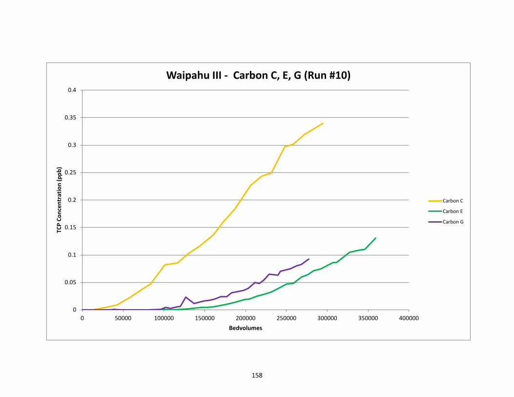
158
0
0.05
0.1
0.15
0.2
0.25
0.3
0.35
0.4
0 50000 100000 150000 200000 250000 300000 350000 400000
TCP
Conc
entr
atio
n (p
pb)
Bedvolumes
Waipahu III - Carbon C, E, G (Run #10)
Carbon C
Carbon E
Carbon G

159
7.2.10 GAC Run #11
Run #11 Waipahu III Sample ID TCP Conc.
(ppb) Carbon A/B K-Infl1 0.550
100 x 120 3.42 mL/min K-Infl2 0.545 120 x 140 4.07 mL/min K-Infl3 0.492 140 x 170 4.82 mL/min K-Infl4 0.500 170 x 200 5.74 mL/min K-Infl5 0.452
Bed Volume 0.355 mL K-Infl6 0.495 TCP Influent 0.506 ppb Infl. Avg 0.506
mg TCP Mass Adsorbed per kg GAC Mass (mg/kg)
Bed - Volumes
1% Breakthru
(ppb)
5% Breakthru
(ppb)
10% Breakthru
(ppb)
1% Breakthru
(ppb)
5% Breakthru
(ppb)
10% Breakthru
(ppb)
Limit Conc.
(ppb) 0.0051 0.0253 0.0506 Limit Conc.
(ppb) 0.0051 0.0253 0.0506 100 x 120 3.478E-04 4.643E-04 5.345E-04 100 x 120 344371 462863 538015 120 x 140 2.790E-04 3.569E-04 4.062E-04 120 x 140 276376 355973 409157 140 x 170 2.635E-04 3.419E-04 3.823E-04 140 x 170 260776 340779 384473 170 x 200 1.944E-04 2.373E-04 2.721E-04 170 x 200 192564 236700 274239
Carbon A/B 100 x 120 mesh
Sample ID Date and Time Time between
consecutive samples (min)
Total Time (min)
Total Time (hrs)
Total Time
(days)
Flow Rate (mL/min)
Treated Vol. (mL)
Bed Volumes
Conc. (ppb) C/CO
mg TCP Mass Adsorbed per kg
GAC Mass (mg/kg)
W100x120-1 10/30/14 14:24 1167 1167 19.5 0.81 1.82 2124 5983 0.000 0.000 6.05E-06 W100x120-2 10/31/14 11:41 1277 2444 40.7 1.70 3.17 6172 17386 0.000 0.000 1.76E-05 W100x120-3 11/1/14 12:48 1507 3951 65.9 2.74 3.69 11733 33050 0.000 0.000 3.34E-05

160
W100x120-4 11/2/14 9:32 1244 5195 86.6 3.61 3.62 16236 45736 0.000 0.000 4.63E-05 W100x120-5 11/3/14 8:00 1348 6543 109.1 4.54 1.49 18245 51393 0.000 0.000 5.20E-05 W100x120-6 11/3/14 20:19 739 7282 121.4 5.06 1.49 19346 54495 0.000 0.000 5.51E-05 W100x120-7 11/4/14 13:11 1012 8294 138.2 5.76 3.26 22645 63788 0.000 0.000 6.45E-05 W100x120-9 11/5/14 10:46 1295 9589 159.8 6.66 3.02 26556 74805 0.000 0.000 7.57E-05
W100x120-10 11/6/14 9:54 1388 10977 183.0 7.62 3.32 31164 87786 0.000 0.000 8.88E-05 W100x120-11 11/7/14 9:06 1392 12369 206.2 8.59 3.76 36398 102529 0.000 0.000 1.04E-04 W100x120-12 11/8/14 14:06 1740 14109 235.2 9.80 3.76 42940 120959 0.000 0.000 1.22E-04 W100x120-13 11/8/14 23:23 557 14666 244.4 10.18 3.68 44990 126732 0.000 0.000 1.28E-04 W100x120-14 11/9/14 9:48 625 15291 254.9 10.62 3.68 47290 133211 0.000 0.000 1.35E-04 W100x120-15 11/9/14 18:58 550 15841 264.0 11.00 3.68 49314 138913 0.002 0.004 1.40E-04 W100x120-17 11/10/14 15:45 1247 17088 284.8 11.87 3.68 53903 151839 0.000 0.000 1.54E-04 W100x120-18 11/11/14 10:18 1113 18201 303.4 12.64 3.68 57999 163377 0.000 0.000 1.65E-04 W100x120-19 11/12/14 8:14 1316 19517 325.3 13.55 3.38 62447 175907 0.000 0.000 1.78E-04 W100x120-20 11/13/14 10:18 1564 21081 351.4 14.64 3.38 67733 190798 0.000 0.000 1.93E-04 W100x120-21 11/14/14 9:05 1367 22448 374.1 15.59 3.31 72258 203544 0.000 0.000 2.06E-04 W100x120-22 11/15/14 14:06 1741 24189 403.2 16.80 3.24 77899 219433 0.000 0.000 2.22E-04 W100x120-23 11/16/14 9:43 1177 25366 422.8 17.62 3.24 81712 230176 0.000 0.000 2.33E-04 W100x120-24 11/17/14 9:35 1432 26798 446.6 18.61 3.59 86853 244657 0.000 0.000 2.47E-04 W100x120-25 11/18/14 9:00 1405 28203 470.1 19.59 3.59 91897 258865 0.000 0.000 2.62E-04 W100x120-26 11/19/14 9:56 1496 29699 495.0 20.62 3.59 97268 273994 0.001 0.002 2.77E-04 W100x120-27 11/20/14 8:54 1378 31077 518.0 21.58 3.47 102049 287463 0.001 0.002 2.91E-04 W100x120-28 11/21/14 11:00 1566 32643 544.1 22.67 3.47 107483 302770 0.001 0.002 3.06E-04 W100x120-29 11/22/14 14:16 1636 34279 571.3 23.80 3.47 113160 318762 0.002 0.004 3.22E-04 W100x120-30 11/24/14 9:36 2600 36879 614.7 25.61 3.47 122182 344176 0.005 0.010 3.48E-04 W100x120-31 11/25/14 9:06 1410 38289 638.2 26.59 3.47 127075 357958 0.009 0.018 3.61E-04 W100x120-32 11/26/14 10:07 1501 39790 663.2 27.63 3.47 132284 372630 0.006 0.012 3.76E-04 W100x120-33 11/28/14 19:28 3441 43231 720.5 30.02 3.47 144224 406264 0.012 0.024 4.09E-04 W100x120-34 11/29/14 16:22 1254 44485 741.4 30.89 3.47 148575 418522 0.010 0.020 4.21E-04 W100x120-35 12/1/14 8:30 2408 46893 781.5 32.56 3.47 156931 442059 0.018 0.036 4.44E-04 W100x120-36 12/2/14 8:53 1463 48356 805.9 33.58 3.47 162008 456359 0.023 0.045 4.58E-04 W100x120-38 12/4/14 9:27 2914 51270 854.5 35.60 3.47 172119 484843 0.033 0.065 4.85E-04 W100x120-39 12/5/14 14:04 1717 52987 883.1 36.80 3.47 178077 501626 0.032 0.063 5.01E-04 W100x120-40 12/7/14 13:12 2828 55815 930.3 38.76 3.47 187890 529268 0.041 0.081 5.27E-04 W100x120-41 12/8/14 9:28 1216 57031 950.5 39.60 3.47 192110 541154 0.054 0.107 5.37E-04
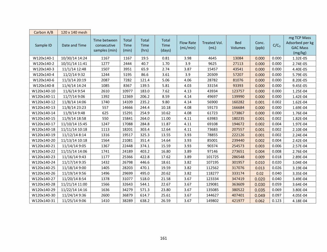
161
Carbon A/B 120 x 140 mesh
Sample ID Date and Time Time between
consecutive samples (min)
Total Time (min)
Total Time (hrs)
Total Time
(days)
Flow Rate (mL/min)
Treated Vol. (mL)
Bed Volumes
Conc. (ppb) C/CO
mg TCP Mass Adsorbed per kg
GAC Mass (mg/kg)
W120x140-1 10/30/14 14:24 1167 1167 19.5 0.81 3.98 4645 13084 0.000 0.000 1.32E-05 W120x140-2 10/31/14 11:41 1277 2444 40.7 1.70 3.9 9625 27113 0.000 0.000 2.74E-05 W120x140-3 11/1/14 12:48 1507 3951 65.9 2.74 3.87 15457 43541 0.000 0.000 4.40E-05 W120x140-4 11/2/14 9:32 1244 5195 86.6 3.61 3.9 20309 57207 0.000 0.000 5.79E-05 W120x140-6 11/3/14 20:19 2087 7282 121.4 5.06 4.06 28782 81076 0.000 0.000 8.20E-05 W120x140-8 11/4/14 14:24 1085 8367 139.5 5.81 4.03 33154 93393 0.000 0.000 9.45E-05
W120x140-10 11/6/14 9:54 2610 10977 183.0 7.62 4.13 43934 123757 0.000 0.000 1.25E-04 W120x140-11 11/7/14 9:06 1392 12369 206.2 8.59 4.14 49697 139990 0.000 0.000 1.42E-04 W120x140-12 11/8/14 14:06 1740 14109 235.2 9.80 4.14 56900 160282 0.001 0.002 1.62E-04 W120x140-13 11/8/14 23:23 557 14666 244.4 10.18 4.08 59173 166684 0.000 0.000 1.69E-04 W120x140-14 11/9/14 9:48 625 15291 254.9 10.62 4.08 61723 173867 0.000 0.000 1.76E-04 W120x140-15 11/9/14 18:58 550 15841 264.0 11.00 4.11 63983 180235 0.001 0.002 1.82E-04 W120x140-17 11/10/14 15:45 1247 17088 284.8 11.87 4.11 69108 194672 0.002 0.004 1.97E-04 W120x140-18 11/11/14 10:18 1113 18201 303.4 12.64 4.11 73683 207557 0.001 0.002 2.10E-04 W120x140-19 11/12/14 8:14 1316 19517 325.3 13.55 3.93 78855 222126 0.001 0.002 2.24E-04 W120x140-20 11/13/14 10:18 1564 21081 351.4 14.64 3.93 85001 239440 0.002 0.004 2.42E-04 W120x140-21 11/14/14 9:05 1367 22448 374.1 15.59 3.93 90374 254573 0.003 0.006 2.57E-04 W120x140-22 11/15/14 14:06 1741 24189 403.2 16.80 3.89 97146 273651 0.004 0.008 2.76E-04 W120x140-23 11/16/14 9:43 1177 25366 422.8 17.62 3.89 101725 286548 0.009 0.018 2.89E-04 W120x140-24 11/17/14 9:35 1432 26798 446.6 18.61 3.82 107195 301957 0.010 0.020 3.04E-04 W120x140-25 11/18/14 9:00 1405 28203 470.1 19.59 3.82 112562 317076 0.013 0.026 3.19E-04 W120x140-26 11/19/14 9:56 1496 29699 495.0 20.62 3.82 118277 333174 0.02 0.040 3.35E-04 W120x140-27 11/20/14 8:54 1378 31077 518.0 21.58 3.67 123334 347419 0.020 0.040 3.49E-04 W120x140-28 11/21/14 11:00 1566 32643 544.1 22.67 3.67 129081 363609 0.030 0.059 3.64E-04 W120x140-29 11/22/14 14:16 1636 34279 571.3 23.80 3.67 135085 380522 0.035 0.069 3.80E-04 W120x140-30 11/24/14 9:36 2600 36879 614.7 25.61 3.67 144627 407401 0.049 0.097 4.05E-04 W120x140-31 11/25/14 9:06 1410 38289 638.2 26.59 3.67 149802 421977 0.062 0.123 4.18E-04

162
Carbon A/B 140 x 170 mesh
Sample ID Date and Time Time between
consecutive samples (min)
Total Time (min)
Total Time (hrs)
Total Time
(days)
Flow Rate (mL/min)
Treated Vol. (mL)
Bed Volumes
Conc. (ppb) C/CO
mg TCP Mass Adsorbed per kg
GAC Mass (mg/kg)
W140x170-1 10/30/14 14:24 1167 1167 19.5 0.81 5.06 5905 16634 0.000 0.000 1.68E-05 W140x170-2 10/31/14 11:41 1277 2444 40.7 1.70 4.87 12124 34152 0.000 0.000 3.45E-05 W140x170-3 11/1/14 12:48 1507 3951 65.9 2.74 4.01 18167 51175 0.000 0.000 5.18E-05 W140x170-4 11/2/14 9:32 1244 5195 86.6 3.61 4.12 23292 65612 0.000 0.000 6.64E-05 W140x170-6 11/3/14 20:19 2087 7282 121.4 5.06 4.76 33226 93596 0.000 0.000 9.47E-05 W140x170-8 11/4/14 14:24 1085 8367 139.5 5.81 4.84 38478 108388 0.000 0.000 1.10E-04 W140x170-9 11/5/14 10:46 1222 9589 159.8 6.66 4.71 44234 124601 0.000 0.000 1.26E-04
W140x170-10 11/6/14 9:54 1388 10977 183.0 7.62 4.86 50979 143603 0.000 0.000 1.45E-04 W140x170-11 11/7/14 9:06 1392 12369 206.2 8.59 4.80 57661 162425 0.000 0.000 1.64E-04 W140x170-12 11/8/14 14:06 1740 14109 235.2 9.80 4.80 66013 185951 0.000 0.000 1.88E-04 W140x170-14 11/9/14 9:48 1182 15291 254.9 10.62 4.74 71615 201734 0.000 0.000 2.04E-04 W140x170-15 11/9/14 18:58 550 15841 264.0 11.00 4.91 74316 209341 0.001 0.002 2.12E-04 W140x170-17 11/10/14 15:45 1247 17088 284.8 11.87 4.91 80439 226588 0.000 0.000 2.29E-04 W140x170-18 11/11/14 10:18 1113 18201 303.4 12.64 4.91 85904 241982 0.002 0.004 2.45E-04 W140x170-19 11/12/14 8:14 1316 19517 325.3 13.55 4.75 92155 259590 0.005 0.010 2.62E-04 W140x170-20 11/13/14 10:18 1564 21081 351.4 14.64 4.75 99584 280517 0.006 0.012 2.83E-04 W140x170-22 11/15/14 14:06 3108 24189 403.2 16.80 4.78 114440 322366 0.016 0.032 3.24E-04 W140x170-23 11/16/14 9:43 1177 25366 422.8 17.62 4.74 120019 338081 0.024 0.047 3.39E-04 W140x170-24 11/17/14 9:35 1432 26798 446.6 18.61 4.69 126735 357000 0.033 0.065 3.57E-04 W140x170-25 11/18/14 9:00 1405 28203 470.1 19.59 4.69 133324 375561 0.042 0.083 3.74E-04 W140x170-26 11/19/14 9:56 1496 29699 495.0 20.62 4.69 140341 395325 0.061 0.121 3.92E-04 W140x170-27 11/20/14 8:54 1378 31077 518.0 21.58 4.64 146734 413337 0.071 0.140 4.08E-04 W140x170-28 11/21/14 11:00 1566 32643 544.1 22.67 4.64 154001 433805 0.083 0.164 4.25E-04

163
Carbon A/B 170 x 200 mesh
Sample ID Date and Time Time between
consecutive samples (min)
Total Time (min)
Total Time (hrs)
Total Time
(days)
Flow Rate (mL/min)
Treated Vol. (mL)
Bed Volumes
Conc. (ppb) C/CO
mg TCP Mass Adsorbed per kg
GAC Mass (mg/kg)
W170x200-1 10/30/14 14:24 1167 1167 19.5 0.81 6.96 8122 22880 0.000 0.000 2.31E-05 W170x200-2 10/31/14 11:41 1277 2444 40.7 1.70 6.21 16052 45218 0.000 0.000 4.57E-05 W170x200-3 11/1/14 12:48 1507 3951 65.9 2.74 5.59 24477 68948 0.000 0.000 6.97E-05 W170x200-4 11/2/14 9:32 1244 5195 86.6 3.61 5.66 31518 88782 0.000 0.000 8.98E-05 W170x200-5 11/3/14 8:00 1348 6543 109.1 4.54 5.65 39134 110236 0.000 0.000 1.11E-04 W170x200-6 11/3/14 20:19 739 7282 121.4 5.06 5.65 43309 121998 0.000 0.000 1.23E-04 W170x200-7 11/4/14 13:11 1012 8294 138.2 5.76 5.59 48966 137933 0.000 0.000 1.39E-04 W170x200-9 11/5/14 10:46 1295 9589 159.8 6.66 5.38 55933 157559 0.000 0.000 1.59E-04
W170x200-10 11/6/14 9:54 1388 10977 183.0 7.62 5.89 64109 180588 0.003 0.006 1.82E-04 W170x200-11 11/7/14 9:06 1392 12369 206.2 8.59 5.94 72377 203879 0.007 0.014 2.06E-04 W170x200-12 11/8/14 14:06 1740 14109 235.2 9.80 5.94 82713 232994 0.023 0.045 2.34E-04 W170x200-14 11/9/14 9:48 1182 15291 254.9 10.62 5.85 89627 252472 0.035 0.069 2.52E-04 W170x200-15 11/9/14 18:58 550 15841 264.0 11.00 5.97 92911 261721 0.042 0.083 2.61E-04 W170x200-16 11/10/14 8:00 782 16623 277.1 11.54 5.97 97580 274872 0.051 0.101 2.73E-04 W170x200-17 11/10/14 15:45 465 17088 284.8 11.87 5.97 100356 282692 0.059 0.117 2.80E-04 W170x200-18 11/11/14 10:18 1113 18201 303.4 12.64 5.97 107000 301409 0.072 0.142 2.96E-04 W170x200-19 11/12/14 8:14 1316 19517 325.3 13.55 5.97 114857 323540 0.093 0.184 3.14E-04 W170x200-20 11/13/14 10:18 1564 21081 351.4 14.64 5.97 124194 349842 0.113 0.223 3.35E-04

164
0.000
0.010
0.020
0.030
0.040
0.050
0.060
0.070
0.080
0.090
0.100
0 100000 200000 300000 400000 500000 600000
TCP
Conc
entr
atio
n (p
pb)
Bedvolumes
Waipahu III - Carbon A/B (Run #11)
100 x 120 mesh
120 x 140 mesh
140 x 170 mesh
170 x 200 mesh

165

166