Embed Size (px)
Citation preview

COMPARATIVE STUDY OF CONVENTIONAL SLAB
AND FLAT PLATE SYSTEM
KAMRUZZAMAN ASIF NAIM HASSAN
SUDEEP DAS TURJA
DEPARTMENT OF CIVIL ENGINEERING
AHSANULLAH UNIVERSITY OF SCIENCE AND TECHNLOLOGY
AUGUST 2017
COMPARATIVE STUDY OF CONVENTIONAL SLAB AND FLAT PLATE SYSTEM
A Thesis
Submitted By: Student ID:
KAMRUZZAMAN ASIF 13.02.03.016
SUDEEP DAS TURJA 13.02.03.046
NAIM HASSAN 13.02.03.048
In partial fulfillment of requirements for the degree of Bachelor of Science in Civil Engineering
Under the Supervision of
Dr. ENAMUR RAHIM LATIFEE Associate Professor
Department of Civil Engineering
AHSANULLAH UNIVERSITY OF SCIENCE AND TECHNOLOGY AUGUST 2017
APPROVED AS TO STYLE AND CONTENT BY
Dr. ENAMUR RAHIM LATIFEE Associate Professor
Department of Civil Engineering
AHSANULLAH UNIVERSITY OF SCIENCE AND TECHNOLOGY
141-142 LOVE ROAD, TEJGAON INDUSTRIAL AREA, DHAKA-1208
AUGUST 2017

I
DECLARATION
The work performed in this thesis for the achievement of the degree of Bachelor
of Science in Civil Engineering is “A study on comparative study of conventional
slab and flat plate system”. The whole work is carried out by the authors under
the strict and friendly supervision of Dr. Enamur Rahim Latifee, Associate
Professor, Department of Civil Engineering, Ahsanullah University of Science and
Technology, Dhaka, Bangladesh.
Neither this thesis nor any part of it is submitted or is being simultaneously
submitted for any degree at any other institutions.
…………………………………. Kamruzzaman Asif
13.02.03.016
…………………………………. Sudeep Das Turja
13.02.03.046
…………………………………. Naim Hassan 13.02.03.048

II
TO OUR BELOVED PARENTS AND TEACHERS

III
ACKNOWLEDGEMENT
There are no proper words to convey our deep gratitude and respect for our
thesis supervisor, Dr. Enamur Rahim Latifee, Associate Professor, Honorable
faculty member, Department of Civil Engineering, Ahsanulllah University of
Science and Technology, for his unrestricted personal guidance throughout this
study and for bringing out the best of our abilities. His supervision,
encouragement, assistance and invaluable suggestion at all stages of the work
made it possible to complete this work.
We would like to express our gratitude to all our teachers and professors who
taught us during the undergraduate time. We would like to thank our classmates
and friends for their continued help and encouragement.
Last but not the least, we deeply thank our parents and siblings for their
unconditional trust, timely encouragement, endless patience and supporting us
spiritually throughout our life.
IV
ABSTRACT
In terms of traditional building design, Slab selection and design becomes the
major issue of concern. In most of the cases design and selection of slab depends
mainly on economy and of course safety. It is often considered as a choice of
selection for less cost and less material while constructing the floor slabs. In this
paper, “Comparative Study of Conventional Slab and Flat plate system”
comparison between conventional slab system (i.e. Two Way Slab with beams)
and Flat plate (i.e. Two Way Slab without beams) is carried out on the basis of
economy. Basically, this paper is focused on the comparison in materials
between the two slab systems. On the other hand, comparison is made on the
total cost (including material cost, laborer cost, form work cost etc.) between
them. For the design purpose “Direct Design Method” is used for both the slab
systems. The design examples were performed on the same interior and exterior
panels with the same long and short dimensions. Before performing the manual
calculations, some excel worksheets were developed according to the ACI 318
codes conforming to “Direct Design Method”. Then the manual calculations
were performed using the same parameters like concrete strength, yield
strength, rebar diameter etc. Finally the results are cross-checked and the
objectives were compared to one another. For example, in manual calculations
minimum thickness of slab is calculated from the thickness table (ACI code 9.5c).
However, in excel worksheets thickness was calculated from four different
criteria such as effective depth, punching shear mechanism, deflection control
mechanism and maximum steel ratio. Different comparison graphs and charts
were developed on the basis of determined results. It is seen that up to a certain
β (long to short span ratio) flat plate is economical over the conventional slab
system. However, with further increase in beta β the traditional slab system
dominates the economy. These comparison results shows a clear overview
enough to select the most economical slab system.
V
TABLE OF CONTENTS
DECLARATION
ACKNOWLEDGEMENT
ABSTRACT
TABLE OF CONTENTS
LIST OF TABLES
LIST OF FIGURES
LIST OF SYMBOLS & ABBREVIATIONS
Chapter 1: INTRODUCTION
Chapter 2: LITERATURE REVIEW
2.1 Two way slab system
2.2 Design procedure
2.3 Direct design method
2.3.1 Limitations of direct design method
2.3.2 Total factored static moment for a span
2.3.3 Negative & positive factored moments
2.3.4 Factored moments in column strips
2.3.5 Factored moments in beam
2.3.6 Factored moments in middle strips
2.4 Slab reinforcement
2.4.1 Details of reinforcement in slabs without beams
2.5 Concrete Floor System
2.5.1 Flat Plate System
Chapter 3: METHODOLOGY & EXPERIMENTAL WORK
3.1 Floor-model selection & design approach
3.2 Flat plate
3.2.1 Design Example 1
I
III
IV
V
VII
VIII
X
1
4
5
5
6
6
7
7
8
11
11
12
13
14
15
16
17
19
20
VI
3.2.2 Design Example 2
3.2.3 Design Example 3
3.2.4 Sample calculation of an exterior frame (without edge
beam) from excel spreadsheet (using DDM)
3.2.5 Sample calculation of an interior frame from excel spread
sheet (using DDM)
3.3 Beam-supported slab
3.3.1 Sample calculation of an exterior frame from excel
spreadsheet (using DDM)
3.3.2 Sample calculation of an interior frame from excel
spreadsheet (using DDM)
3.4 Design Example of two way beam supported slab (using
Moment coefficient method)
Chapter 4: RESULTS & DISCUSSION
Chapter 5: CONCLUSION
5.1 Limitations
5.2 Recommendations
5.3 Conclusion
REFERENCES
31
41
50
51
53
54
56
58
62
78
79
80
81
82
VII
LIST OF TABLES
Table no. Name of the Table Page no.
2.1 Negative & Positive Factored Moments 8
2.2 Interior Negative Factored Moments in Column Strips 8
2.3 Exterior negative factored moments 9
2.4 Positive Factored Moments in Column Strips 10
3.1 Panel sizes of the floor models been designed 17
3.2 Minimum thickness of slabs 21
3.3 Distribution of total span moments 22
3.4 Percentage distribution of interior neg. moments 23
3.5 Percentage distribution of pos. moments 24
3.6 Percentage distribution of exterior neg. moments 25
3.7 Assignment of M0 to positive and negative moment regions in the exterior span
43
4.1 Comparison table for long to short span ratio, β = 1.00 63
4.2 Comparison table for long to short span ratio, β = 1.25 64
4.3 Comparison table for long to short span ratio, β = 1.50 65
4.4 Comparison table for long to short span ratio, β = 1.75 66
4.5 Comparison table for long to short span ratio, β = 2.00 67
4.6 Comparison table for long to short span ratio, β =1.24 68
VIII
LIST OF FIGURES
Figure no. Name of the figure Page no.
2.1 Composite section 10
2.2 Ductile design Concept 12
2.3 Minimum extensions for reinforcement in slab without
beams
13
3.1 Plan of column-layout to be designed 17
3.2 Division of slab into frames for design 18
3.3 Typical exterior panel (with edge beam) 20
3.4 Edge beam dimension 21
3.5 Edge beam dimension for βt calculation 24
3.6 Assignment of M0 to positive and negative moment regions in the exterior span
27
3.7 Reinforcement Details 30
3.8 Typical interior frame 31
3.9 Assignment of M0 to positive and negative moment regions in the interior span
34
3.10 Assignment of M0 to positive and negative moment
regions in the interior span
36
3.11 Typical Exterior Panel (without edge beam)
41
3.12 Assignment of M0 to positive and negative moment regions in the exterior span
46
3.13 Reinforcement Details 49
3.14 Reinforcement details of slab in plan 61
4.1 Cost comparison chart for β =1.00 69
4.2 Steel comparison chart for β =1.00 69
IX
4.3 Concrete comparison chart for β =1.00 70
4.4 Cost comparison chart for β =1.25 70
4.5 Steel comparison chart for β =1.25 71
4.6 Concrete comparison chart for β =1.25 71
4.7 Cost comparison chart for β =1.5 72
4.8 Steel comparison chart for β =1.5 72
4.9 Concrete comparison chart for β =1.5 73
4.10 Cost comparison chart for β =1.75 73
4.11 Steel comparison chart for β =1.75 74
4.12 Concrete comparison chart for β =1.75 74
4.13 Cost comparison chart for β =2.00 75
4.14 Steel comparison chart for β =2.00 75
4.15 Concrete comparison chart for β =2.00 75
4.16 Cost vs. β graph for short span of 10 ft. 76
4.17 Cost vs. β graph for short span of 15 ft. 76
4.18 Cost comparison chart for 31’x25’panel 77
4.19 Steel comparison chart for 31’x25’panel 77
4.20 Concrete comparison chart for 31’x25’panel 77
X
LIST OF SYMBOLS AND ABBREVIATIONS ACI = American Concrete Institute. ASCE = American Society of Civil Engineers. BNBC = Bangladesh National Building Code. IBC = International Building Code. UBC = Uniform Building Code. EN = Euro/British Code. DDM =Direct Design Method. EFM = Equivalent Frame Method. MCM=Moment Coefficient Method DL = Dead load. LL = Live load. l = Length of span. ln = Length of clear span. lA = Length of clear span in short direction. lB = Length of clear span in long direction. As = Area of steel. f’c = Compressive strength of concrete. fy = Grade/Yield strength of steel. psi =Pound per square inch psf = Pound per square foot ksi =Kilo pound per square inch ksf = Kio pound per square foot h = Thickness of slab. bw =beam width hw = clear height α = Stiffness ratio of beam to slab. β = Long clear span to short clear span ratio E = Modulus of elasticity. I = Moment of inertia. P = Perimeter.
𝜌 = Steel ratio.

1
Chapter 1
INTRODUCTION
2
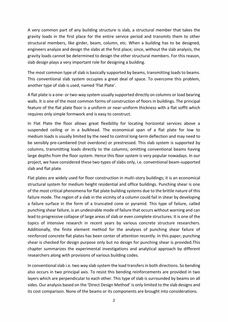
A very common part of any building structure is slab, a structural member that takes the
gravity loads in the first place for the entire service period and transmits them to other
structural members, like girder, beam, column, etc. When a building has to be designed,
engineers analyze and design the slabs at the first place; since, without the slab analysis, the
gravity loads cannot be determined to design the other structural members. For this reason,
slab design plays a very important role for designing a building.
The most common type of slab is basically supported by beams, transmitting loads to beams.
This conventional slab system occupies a great deal of space. To overcome this problem,
another type of slab is used, named ‘Flat Plate’.
A flat plate is a one- or two-way system usually supported directly on columns or load bearing
walls. It is one of the most common forms of construction of floors in buildings. The principal
feature of the flat plate floor is a uniform or near-uniform thickness with a flat soffit which
requires only simple formwork and is easy to construct.
In Flat Plate the floor allows great flexibility for locating horizontal services above a
suspended ceiling or in a bulkhead. The economical span of a flat plate for low to
medium loads is usually limited by the need to control long-term deflection and may need to
be sensibly pre-cambered (not overdone) or prestressed. This slab system is supported by
columns, transmitting loads directly to the columns; omitting conventional beams having
large depths from the floor system. Hence this floor system is very popular nowadays. In our
project, we have considered these two types of slabs only, i.e. conventional beam-supported
slab and flat plate.
Flat plates are widely used for floor construction in multi-story buildings; it is an economical
structural system for medium height residential and office buildings. Punching shear is one
of the most critical phenomena for flat plate building systems due to the brittle nature of this
failure mode. The region of a slab in the vicinity of a column could fail in shear by developing
a failure surface in the form of a truncated cone or pyramid. This type of failure, called
punching shear failure, is an undesirable mode of failure that occurs without warning and can
lead to progressive collapse of large areas of slab or even complete structures. It is one of the
topics of intensive research in recent years by various concrete structure researchers.
Additionally, the finite element method for the analyses of punching shear failure of
reinforced concrete flat plates has been center of attention recently. In this paper, punching
shear is checked for design purpose only but no design for punching shear is provided.This
chapter summarizes the experimental investigations and analytical approach by different
researchers along with provisions of various building codes.
In conventional slab i.e. two way slab system the load transfers in both directions. So bending
also occurs in two principal axis. To resist this bending reinforcements are provided in two
layers which are perpendicular to each other. This type of slab is surrounded by beams on all
sides. Our analysis based on the ‘Direct Design Method’ is only limited to the slab designs and
its cost comparison. None of the beams or its components are brought into considerations.
3
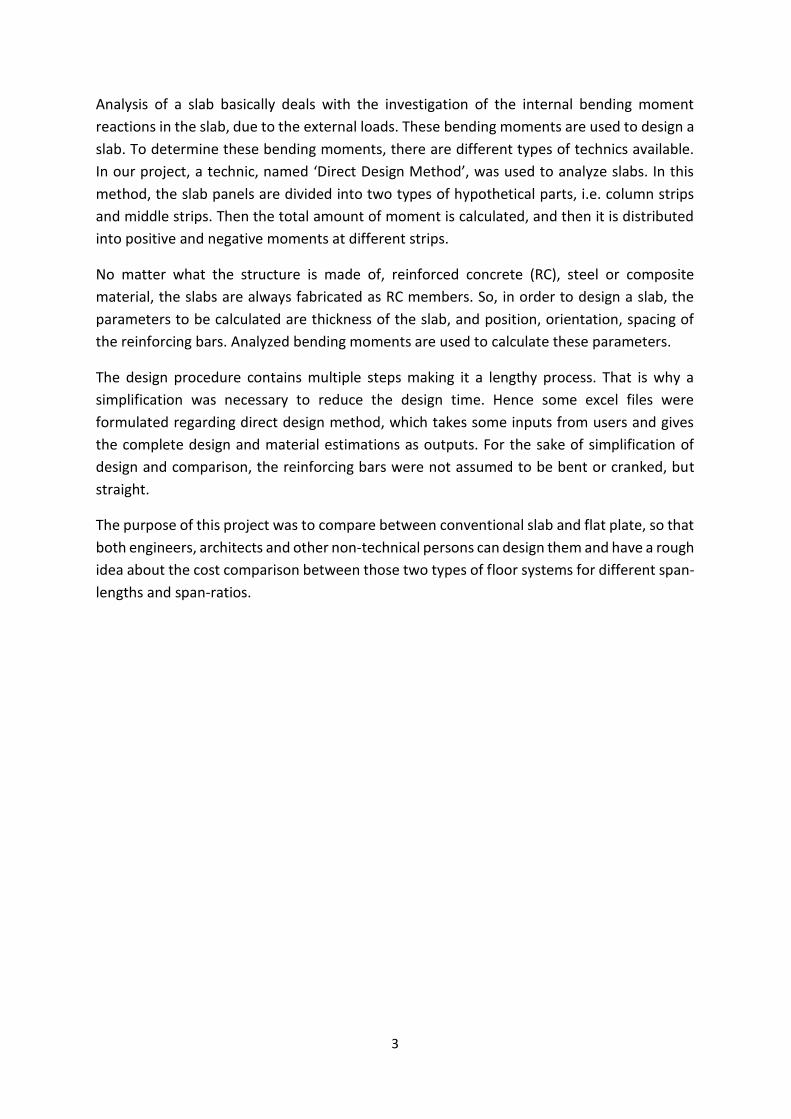
Analysis of a slab basically deals with the investigation of the internal bending moment
reactions in the slab, due to the external loads. These bending moments are used to design a
slab. To determine these bending moments, there are different types of technics available.
In our project, a technic, named ‘Direct Design Method’, was used to analyze slabs. In this
method, the slab panels are divided into two types of hypothetical parts, i.e. column strips
and middle strips. Then the total amount of moment is calculated, and then it is distributed
into positive and negative moments at different strips.
No matter what the structure is made of, reinforced concrete (RC), steel or composite
material, the slabs are always fabricated as RC members. So, in order to design a slab, the
parameters to be calculated are thickness of the slab, and position, orientation, spacing of
the reinforcing bars. Analyzed bending moments are used to calculate these parameters.
The design procedure contains multiple steps making it a lengthy process. That is why a
simplification was necessary to reduce the design time. Hence some excel files were
formulated regarding direct design method, which takes some inputs from users and gives
the complete design and material estimations as outputs. For the sake of simplification of
design and comparison, the reinforcing bars were not assumed to be bent or cranked, but
straight.
The purpose of this project was to compare between conventional slab and flat plate, so that
both engineers, architects and other non-technical persons can design them and have a rough
idea about the cost comparison between those two types of floor systems for different span-
lengths and span-ratios.

4
Chapter 2
LITERATURE REVIEW

5
2.1 Two Way Slab System
A slab system supported by columns or walls, dimensions c1, c2 and ln shall be based on an
effective support area defined by the intersection of the bottom surface of the slab, or of
the drop panel or shear cap if present, with the largest right circular cone, right pyramid, or
tapered wedge whose surfaces are located within the column and the capital or bracket and
are oriented no greater than 45 degrees to the axis of the column.
2.2 Design Procedure
A slab system shall be designed by any procedure satisfying conditions of equilibrium any
geometric compatibility if it is shown that at every section is at least equal to the required
strength and all serviceability conditions including limits on deflections are met.
Design of a slab system for gravity loads including the slab beams (if any) between supports
and supporting columns or walls forming orthogonal frames, by either Direct Design
Method or the Equivalent Frame Method.
For gravity load analysis of two-way slab systems, two analysis methods are given in section
13.6 and 13.7 in ACI 318-11. The specific provisions of both design methods are limited in
application to orthogonal frames subjected to gravity loads only. Both methods apply to
two-way slabs with beams as well as to flat slabs and flat plates. In both methods the
distribution of moments to the critical sections of the slab reflects the effects of reduces
stiffness of elements due to cracking and support geometry.
6
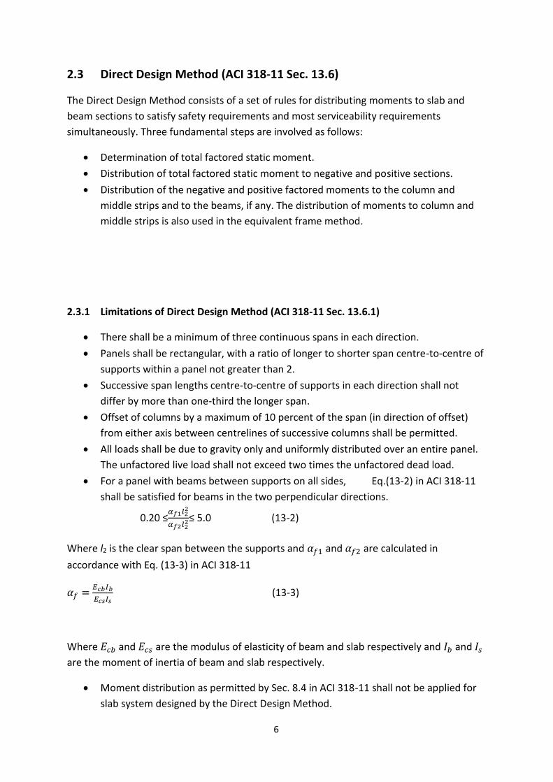
2.3 Direct Design Method (ACI 318-11 Sec. 13.6)
The Direct Design Method consists of a set of rules for distributing moments to slab and
beam sections to satisfy safety requirements and most serviceability requirements
simultaneously. Three fundamental steps are involved as follows:
Determination of total factored static moment.
Distribution of total factored static moment to negative and positive sections.
Distribution of the negative and positive factored moments to the column and
middle strips and to the beams, if any. The distribution of moments to column and
middle strips is also used in the equivalent frame method.
2.3.1 Limitations of Direct Design Method (ACI 318-11 Sec. 13.6.1)
There shall be a minimum of three continuous spans in each direction.
Panels shall be rectangular, with a ratio of longer to shorter span centre-to-centre of
supports within a panel not greater than 2.
Successive span lengths centre-to-centre of supports in each direction shall not
differ by more than one-third the longer span.
Offset of columns by a maximum of 10 percent of the span (in direction of offset)
from either axis between centrelines of successive columns shall be permitted.
All loads shall be due to gravity only and uniformly distributed over an entire panel.
The unfactored live load shall not exceed two times the unfactored dead load.
For a panel with beams between supports on all sides, Eq.(13-2) in ACI 318-11
shall be satisfied for beams in the two perpendicular directions.
0.20 ≤𝛼𝑓1𝑙2
2
𝛼𝑓2𝑙22≤ 5.0 (13-2)
Where l2 is the clear span between the supports and 𝛼𝑓1 and 𝛼𝑓2 are calculated in
accordance with Eq. (13-3) in ACI 318-11
𝛼𝑓 = 𝐸𝑐𝑏𝐼𝑏
𝐸𝑐𝑠𝐼𝑠 (13-3)
Where 𝐸𝑐𝑏 and 𝐸𝑐𝑠 are the modulus of elasticity of beam and slab respectively and 𝐼𝑏 and 𝐼𝑠
are the moment of inertia of beam and slab respectively.
Moment distribution as permitted by Sec. 8.4 in ACI 318-11 shall not be applied for
slab system designed by the Direct Design Method.
7
Variations from the limitations of 13.6.1 shall be permitted if demonstrated by
analysis that requirements of 13.5.1 are satisfied.
2.3.2 Total Factored Static Moment for A Span (ACI 318-11 Sec. 13.6.2)
Total factored static moment, Mo, for a span shall be determined in a strip bounded laterally
by centreline of panel on each side of centreline of supports.
Absolute sum of positive and average negative factored moments in each direction shall not
be less than
𝑙𝑛=transverse width of the strip.
𝑙2= clear span between columns
2.3.3 Negative & Positive Factored Moments (ACI 318-11 Sec. 13.6.3)
Negative factored moments shall be located at the face of rectangular supports. Circular or
regular polygon shaped supports shall be treated as square supports with the same area.
In an interior span total static moment, Mo shall be distributed as follows:
Negative factored moment ------------------ 0.65
Positive factored moment ------------------- 0.35
In an end span total factored static moment, Mo shall be distributed as follows:
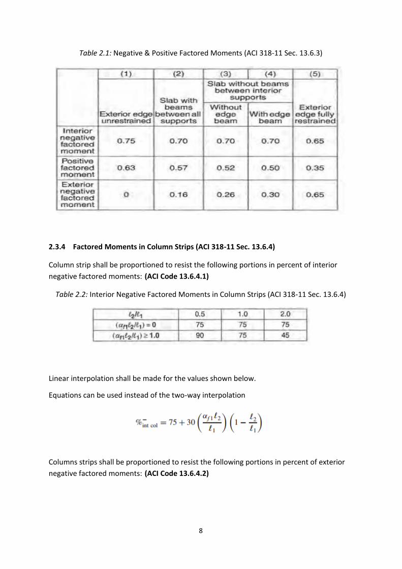
8
Table 2.1: Negative & Positive Factored Moments (ACI 318-11 Sec. 13.6.3)
2.3.4 Factored Moments in Column Strips (ACI 318-11 Sec. 13.6.4)
Column strip shall be proportioned to resist the following portions in percent of interior
negative factored moments: (ACI Code 13.6.4.1)
Table 2.2: Interior Negative Factored Moments in Column Strips (ACI 318-11 Sec. 13.6.4)
Linear interpolation shall be made for the values shown below.
Equations can be used instead of the two-way interpolation
Columns strips shall be proportioned to resist the following portions in percent of exterior
negative factored moments: (ACI Code 13.6.4.2)
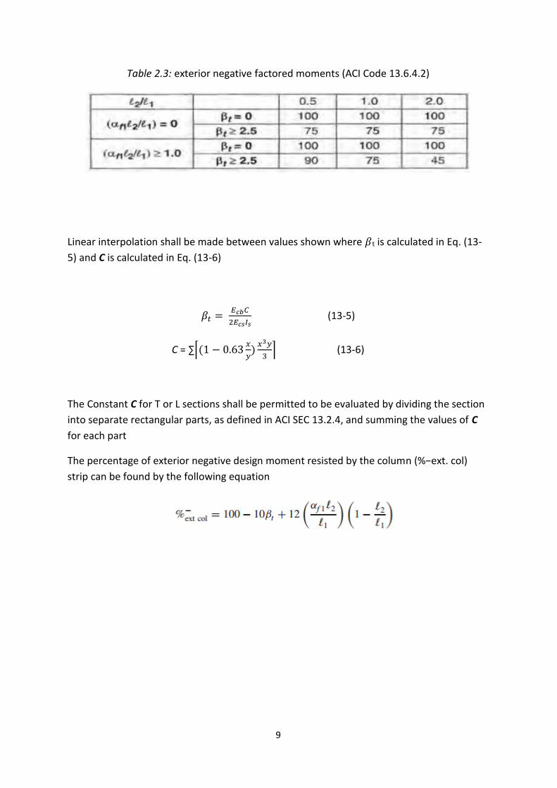
9
Table 2.3: exterior negative factored moments (ACI Code 13.6.4.2)
Linear interpolation shall be made between values shown where 𝛽t is calculated in Eq. (13-
5) and C is calculated in Eq. (13-6)
𝛽𝑡 = 𝐸𝑐𝑏𝐶
2𝐸𝑐𝑠𝐼𝑠 (13-5)
C = ∑⌈(1 − 0.63𝑥
𝑦)
𝑥3𝑦
3⌉ (13-6)
The Constant C for T or L sections shall be permitted to be evaluated by dividing the section
into separate rectangular parts, as defined in ACI SEC 13.2.4, and summing the values of C
for each part
The percentage of exterior negative design moment resisted by the column (%−ext. col)
strip can be found by the following equation
10
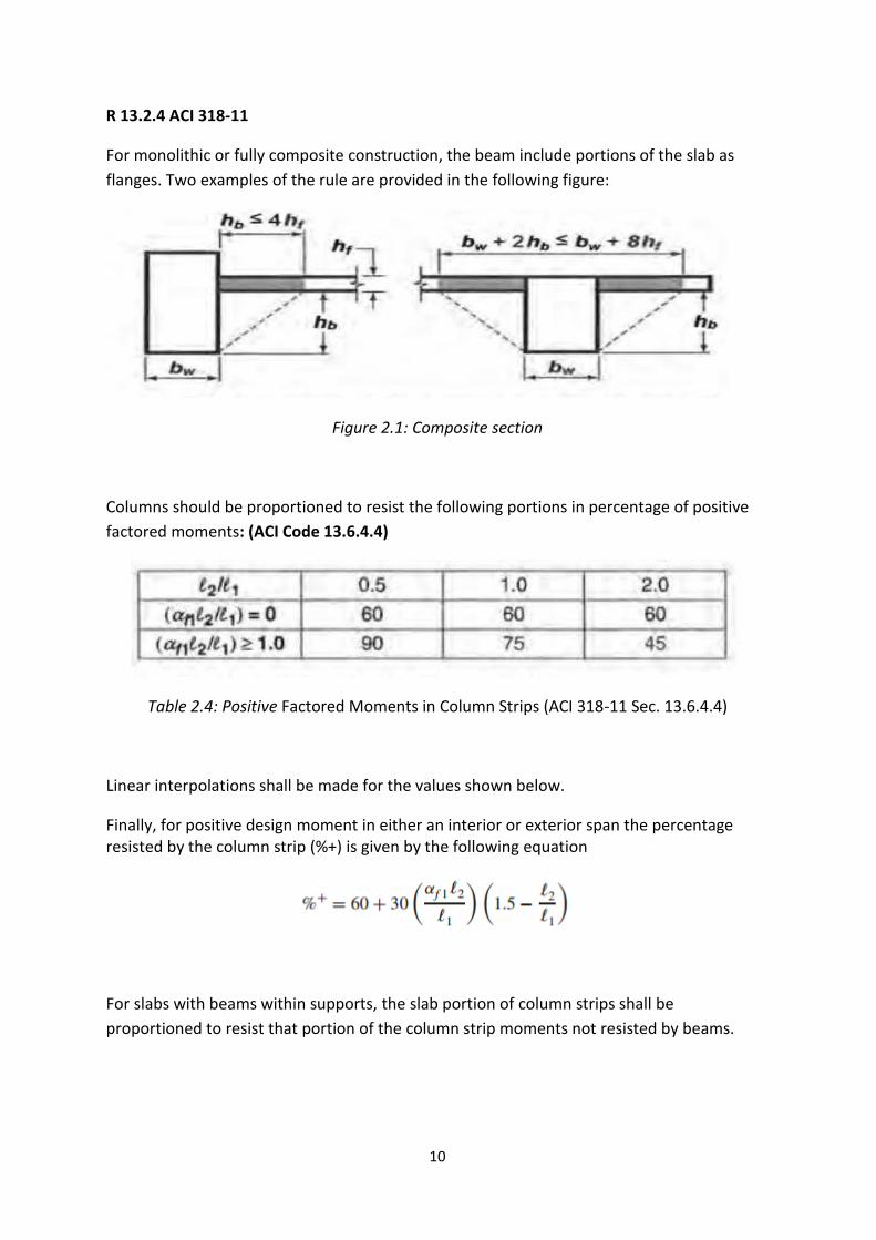
R 13.2.4 ACI 318-11
For monolithic or fully composite construction, the beam include portions of the slab as
flanges. Two examples of the rule are provided in the following figure:
Figure 2.1: Composite section
Columns should be proportioned to resist the following portions in percentage of positive
factored moments: (ACI Code 13.6.4.4)
Table 2.4: Positive Factored Moments in Column Strips (ACI 318-11 Sec. 13.6.4.4)
Linear interpolations shall be made for the values shown below.
Finally, for positive design moment in either an interior or exterior span the percentage resisted by the column strip (%+) is given by the following equation
For slabs with beams within supports, the slab portion of column strips shall be
proportioned to resist that portion of the column strip moments not resisted by beams.

11
2.3.5 Factored Moments in Beam (ACI 318-11 Sec. 13.6.5)
Beams between supports shall be proportioned to resist 85 percent of column strip
moments if 𝛼f1l2/l1 is equal to or greater than 1.
For values of 𝛼f1l2/l1 between 1.0 and zero, proportion of column strip moments resisted by
beams shall be obtained by linear interpolation between 85 and zero percent.
2.3.6 Factored Moments in Middle Strips (ACI 318-11 Sec. 13.6.6)
That proportion of positive and negative moments not resisted by column strips shall be
proportionately assigned to its two half middle strips.
Each middle strip shall be proportioned to resist the sum of the moments assigned to its
two half middle strips.
A middle strip adjacent to and parallel with a wall supported edge shall be proportioned to
resist the twice the moment assigned to the half middle strip corresponding to the first row
of interior supports.
12
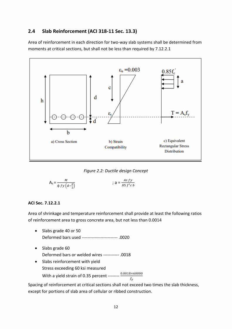
2.4 Slab Reinforcement (ACI 318-11 Sec. 13.3)
Area of reinforcement in each direction for two-way slab systems shall be determined from
moments at critical sections, but shall not be less than required by 7.12.2.1
Figure 2.2: Ductile design Concept
As = 𝑀
ɸ 𝑓𝑦 (𝑑−𝑎
2) ; a =
𝐴𝑠 𝑓𝑦
.85 𝑓′𝑐 𝑏
ACI Sec. 7.12.2.1
Area of shrinkage and temperature reinforcement shall provide at least the following ratios
of reinforcement area to gross concrete area, but not less than 0.0014
Slabs grade 40 or 50
Deformed bars used ------------------------- .0020
Slabs grade 60
Deformed bars or welded wires ----------- .0018
Slabs reinforcement with yield
Stress exceeding 60 ksi measured
With a yield strain of 0.35 percent -------- 0.0018×60000
𝑓𝑦
Spacing of reinforcement at critical sections shall not exceed two times the slab thickness,
except for portions of slab area of cellular or ribbed construction.
13
Positive moment reinforcement perpendicular to a discontinuous edge shall extend to the
edge of the slab and have embedment, straight or hooked, at least 6 inch in spandrel
beams, columns or walls.
Negative moment reinforcement perpendicular to discontinuous edge shall be bent, hooked
or otherwise anchored in spandrel beams, columns or walls and shall be developed at the
face of the support.
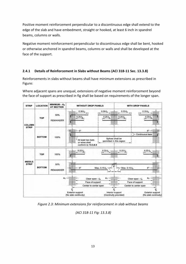
2.4.1 Details of Reinforcement in Slabs without Beams (ACI 318-11 Sec. 13.3.8)
Reinforcements in slabs without beams shall have minimum extensions as prescribed in Figure:
Where adjacent spans are unequal, extensions of negative moment reinforcement beyond the face of support as prescribed in fig shall be based on requirements of the longer span.
Figure 2.3: Minimum extensions for reinforcement in slab without beams
(ACI 318-11 Fig: 13.3.8)

14
2.5 Concrete Floor System
Numerous types of cast-in-place and precast concrete floor systems are available to satisfy
virtually any span and loading condition. Reinforced concrete allows a wide range of
structural options and provides cost-effective solutions for multitude of situations-from
residential buildings with moderate live loads and spans of about 25 ft. to commercial
buildings with heavier live loads and spans ranging from 40 ft. to 50 ft. and beyond. Shorter
floor-to-floor heights and inherent fire and vibration resistance are only a few of the many
advantages that concrete floor system offer, resulting in significant reductions in both
structural and non-structural costs.
Since the cost of the floor system can be a major part of the structural cost of a building,
selecting the most effective system for a given set of constraints is vital in achieving overall
economy. This is especially important for buildings of low-and medium heights and for
buildings subjected to relatively low wind or seismic loads, since the cost of lateral load
resistance in these cases is minimal. The information provided below will help in selecting
an economical cast-in-place concrete floor system for variety of span lengths and
superimposed gravity loads.
The main components of cast-in-place concrete floor systems are concrete, reinforcement
and formwork. The cost of concrete, including placing and finishing, usually accounts for
about 30% to 35% of the overall cost of the floor system. Having the greatest influence on
the overall cost of the floor system, which is about 45% to 55% of the total cost. The
reinforcing steel has the lowest influence on the overall cost.
To achieve overall economy, designers should satisfy the following three basic principles of
formwork economy:
Specify readily available standard form sizes.
Repeat sizes and shapes of the concrete members whenever possible.
Strive for simple formwork.
15
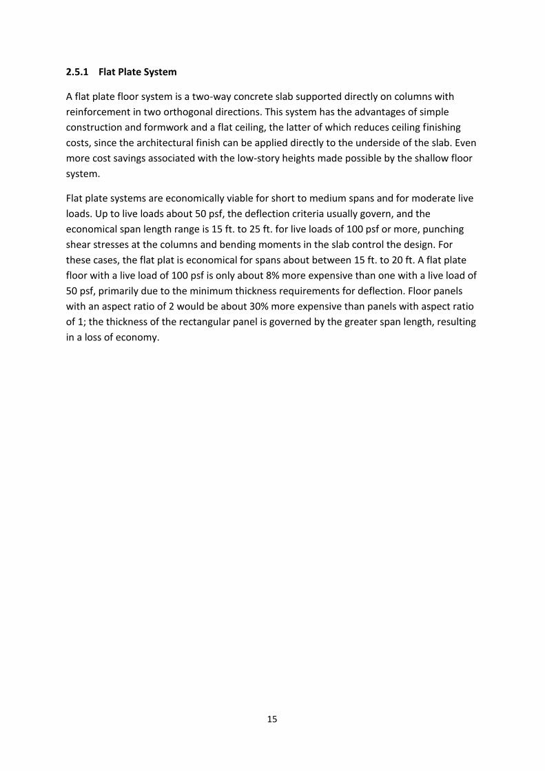
2.5.1 Flat Plate System
A flat plate floor system is a two-way concrete slab supported directly on columns with
reinforcement in two orthogonal directions. This system has the advantages of simple
construction and formwork and a flat ceiling, the latter of which reduces ceiling finishing
costs, since the architectural finish can be applied directly to the underside of the slab. Even
more cost savings associated with the low-story heights made possible by the shallow floor
system.
Flat plate systems are economically viable for short to medium spans and for moderate live
loads. Up to live loads about 50 psf, the deflection criteria usually govern, and the
economical span length range is 15 ft. to 25 ft. for live loads of 100 psf or more, punching
shear stresses at the columns and bending moments in the slab control the design. For
these cases, the flat plat is economical for spans about between 15 ft. to 20 ft. A flat plate
floor with a live load of 100 psf is only about 8% more expensive than one with a live load of
50 psf, primarily due to the minimum thickness requirements for deflection. Floor panels
with an aspect ratio of 2 would be about 30% more expensive than panels with aspect ratio
of 1; the thickness of the rectangular panel is governed by the greater span length, resulting
in a loss of economy.

16
Chapter 3
METHODOLOGY &
EXPERIMENTAL
WORK
17
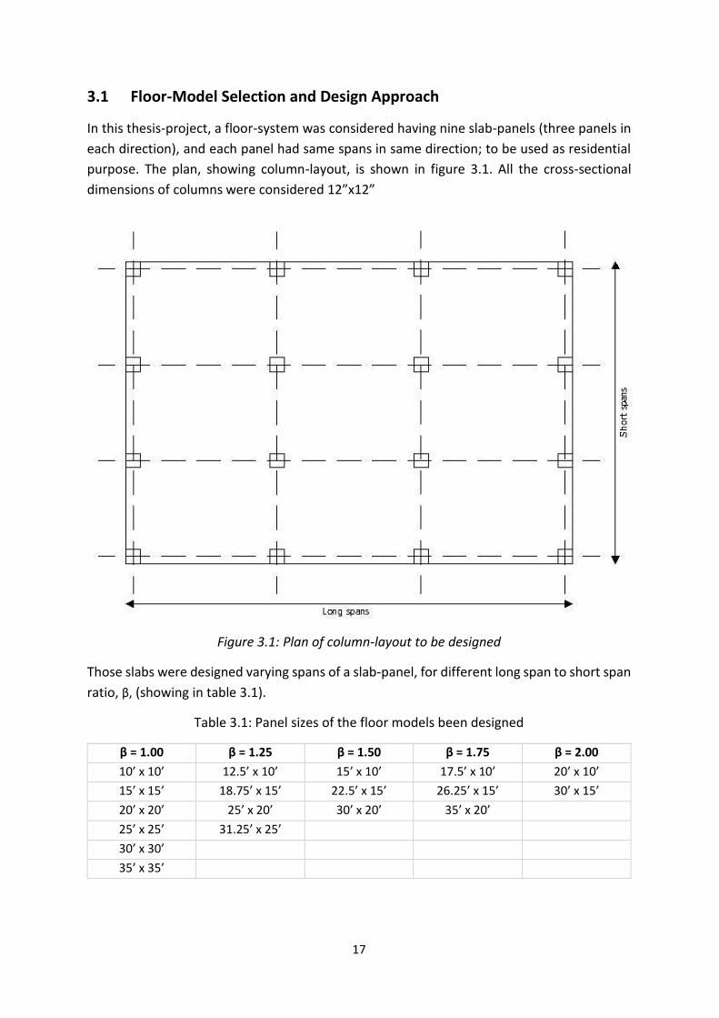
3.1 Floor-Model Selection and Design Approach
In this thesis-project, a floor-system was considered having nine slab-panels (three panels in
each direction), and each panel had same spans in same direction; to be used as residential
purpose. The plan, showing column-layout, is shown in figure 3.1. All the cross-sectional
dimensions of columns were considered 12”x12”
Figure 3.1: Plan of column-layout to be designed
Those slabs were designed varying spans of a slab-panel, for different long span to short span
ratio, β, (showing in table 3.1).
Table 3.1: Panel sizes of the floor models been designed
β = 1.00 β = 1.25 β = 1.50 β = 1.75 β = 2.00
10’ x 10’ 12.5’ x 10’ 15’ x 10’ 17.5’ x 10’ 20’ x 10’
15’ x 15’ 18.75’ x 15’ 22.5’ x 15’ 26.25’ x 15’ 30’ x 15’
20’ x 20’ 25’ x 20’ 30’ x 20’ 35’ x 20’
25’ x 25’ 31.25’ x 25’
30’ x 30’
35’ x 35’
18
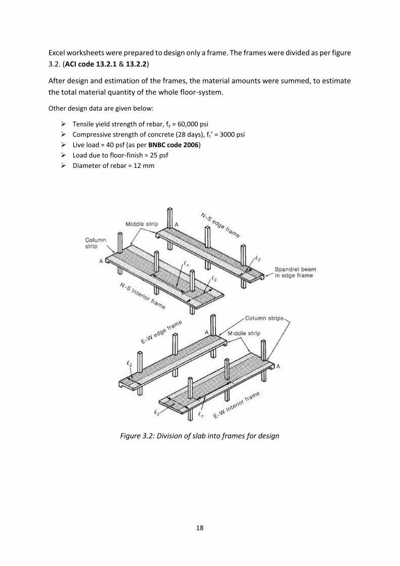
Excel worksheets were prepared to design only a frame. The frames were divided as per figure
3.2. (ACI code 13.2.1 & 13.2.2)
After design and estimation of the frames, the material amounts were summed, to estimate
the total material quantity of the whole floor-system.
Other design data are given below:
Tensile yield strength of rebar, fy = 60,000 psi
Compressive strength of concrete (28 days), fc’ = 3000 psi
Live load = 40 psf (as per BNBC code 2006)
Load due to floor-finish = 25 psf
Diameter of rebar = 12 mm
Figure 3.2: Division of slab into frames for design
19
3.2 Flat Plate
Step 1: At first, we studied how to design a flat-plate by Direct Design Method, from text-
books and ACI codes.
Step 2: We designed one interior frame and one exterior frame, by hand calculation, to get
familiar with the design procedure. Those calculations are shown in article 3.2.1 and 3.2.2.
Step 3: After understanding the design procedure properly, we started to formulate excel
spreadsheets, based on what we learnt on previous two steps. Two separate spreadsheets
were formulated to design both interior and exterior frames. Those were prepared in way
that it would take c/c span lengths of a frame, largest spans along both axes of the floor,
column cross-sections, slab-thickness, and different design data as inputs; and would give
outputs: slab thickness, bending-moments in both column and middle strips, rebar detailing
(showing rebar diameter, spacing and cut-off lengths), width of column and middle strips,
and estimated materials (weight of reinforcing steel and volume of concrete).
Step 4: As per table 3.1, inputs were put in the spreadsheets to design and estimate the floors.
The first task to work with the spreadsheets was the determination of the slab thickness,
which were based on four criteria:
Minimum thickness to control deflections, established by ACI code: table 9.5(c)
Minimum effective depth for maximum reinforcement ratios, established by ACI
code 10.3.5
Minimum effective depth required for punching shear capacity of concrete,
established by ACI code 11.11.2
Minimum thickness to satisfy ACI code 9.5.3.2(a)
The worksheets were formulated in such a way that users not only can input the slab
thickness, but also see suggested thicknesses satisfying those four conditions (based on the
input thickness). So, at first, an assumed thickness had been input in the worksheets for the
frame having the largest clear span of the floor, and then observing the other suggestions,
input thickness was being changed simultaneously. At the last stage, a thickness had been
input that satisfied all the criteria, and not exceeding them. Then that thickness was put in
the worksheet for all the frames of a same floor.
Step 5: After designing all the frames and estimation of a floor, estimated material quantities
from outputs of those spreadsheets, were summed to estimate total material quantity for
the designed floor-system. By the same approach, all the floors were estimated shown in
table 3.1.
Step 6: Using all the estimated material quantities for different floors, were used to calculate
costs. For cost analysis, the considered types of costs are:
20
• Material cost
Mild steel rebar was used as reinforcement. The cost-rate of mild steel rebar, found
in the market, was BDT 50,000 per metric ton. The cost-rate for Ready Mix Concrete
(RMC), found in the market, was BDT 250 per cft. [Shah Cement]
• Form-work cost
The cost-rate assumed was BDT 44.40 per cft.
• Labor cost
The cost-rate assumed was BDT 1.00 per cft.
Those three types of costs were summed and expressed as per square-feet of floor area,
which were the total cost for a certain floor.
Step 7: Using the total material quantities and total costs, different column-charts had been
developed to interpret cost analysis. Those charts are shown in chapter 5.
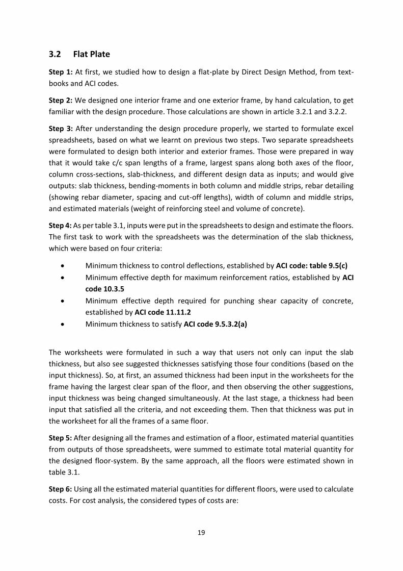
3.2.1 Design Example
Compute the positive and negative moments in the column and middle strips of the
exterior panel of the flat plate between columns B and E in Fig-1. The slab supports a
superimposed dead load of 25 psf and a service live load of 50 psf. The beam is 12 inch wide
by 16 inch in overall depth and is cast monolithically with the slab
Figure 3.3: Typical Exterior Panel (with edge beam)
21
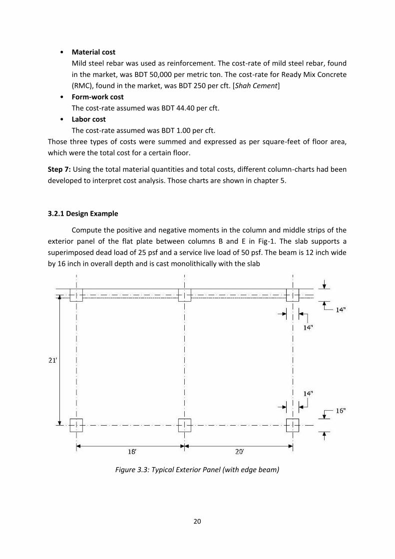
Figure 3.4: Edge Beam dimension
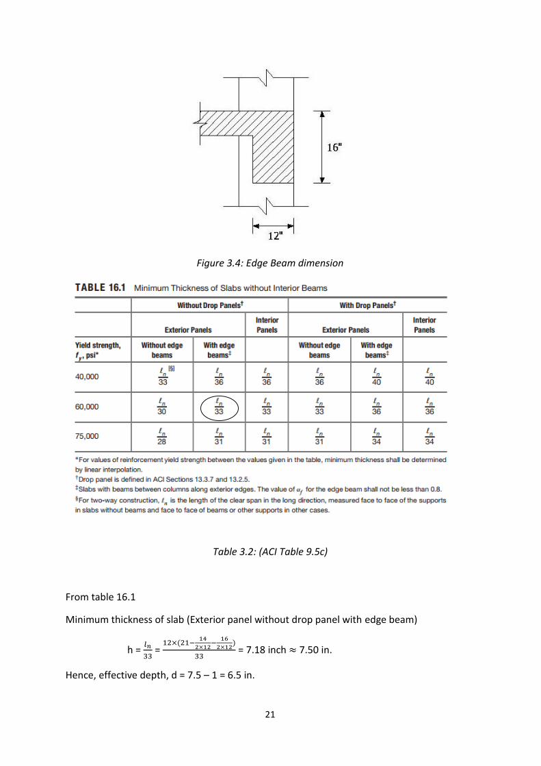
Table 3.2: (ACI Table 9.5c)
From table 16.1
Minimum thickness of slab (Exterior panel without drop panel with edge beam)
h = 𝑙𝑛
33 =
12×(21−14
2×12−
16
2×12)
33 = 7.18 inch ≈ 7.50 in.
Hence, effective depth, d = 7.5 – 1 = 6.5 in.
22
Factored load = 1.2× (7.50
12× 150 + 25) + 1.6 × 50 = 0.223 ksf
Moments in the long span of the slab:
Statical Moment,
𝑙𝑛= transverse width of the strip.
𝑙2= clear span between columns
𝑙𝑛= 21− 14
2×12−
16
2×12= 19.75ft
𝑙2= 19ft
Mo = 0.223×19×19.752
8 = 206.58 k-ft
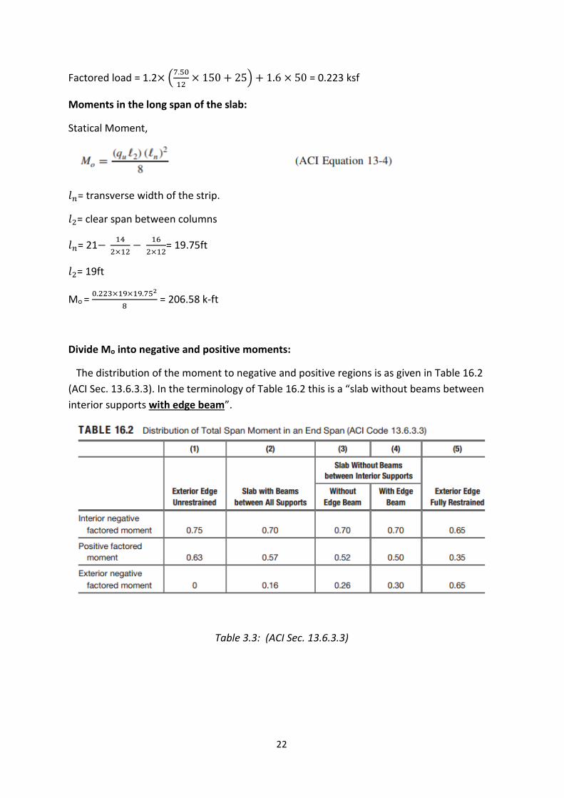
Divide Mo into negative and positive moments:
The distribution of the moment to negative and positive regions is as given in Table 16.2
(ACI Sec. 13.6.3.3). In the terminology of Table 16.2 this is a “slab without beams between
interior supports with edge beam”.
Table 3.3: (ACI Sec. 13.6.3.3)
23
From the Table 16.2, the total moment is divided as
Interior negative Mo= 0.70Mo = 0.70 x 206.58 = 144.61 k-ft
Positive Mo = 0.50 Mo = 0.50 x 206.58 = 103.29 k-ft
Exterior negative Mo= 0.30 Mo= 0.30 x 206.58 = 61.98 k-ft
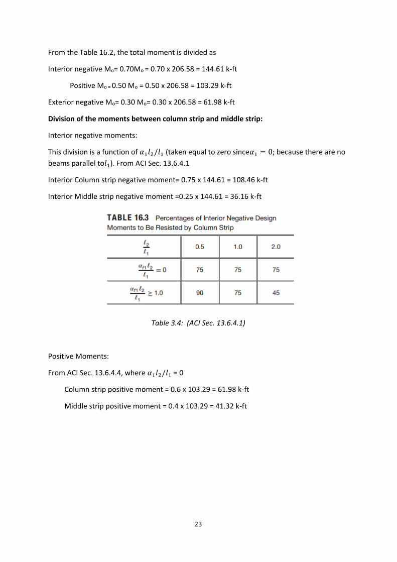
Division of the moments between column strip and middle strip:
Interior negative moments:
This division is a function of 𝛼1𝑙2/𝑙1 (taken equal to zero since𝛼1 = 0; because there are no
beams parallel to𝑙1). From ACI Sec. 13.6.4.1
Interior Column strip negative moment= 0.75 x 144.61 = 108.46 k-ft
Interior Middle strip negative moment =0.25 x 144.61 = 36.16 k-ft
Table 3.4: (ACI Sec. 13.6.4.1)
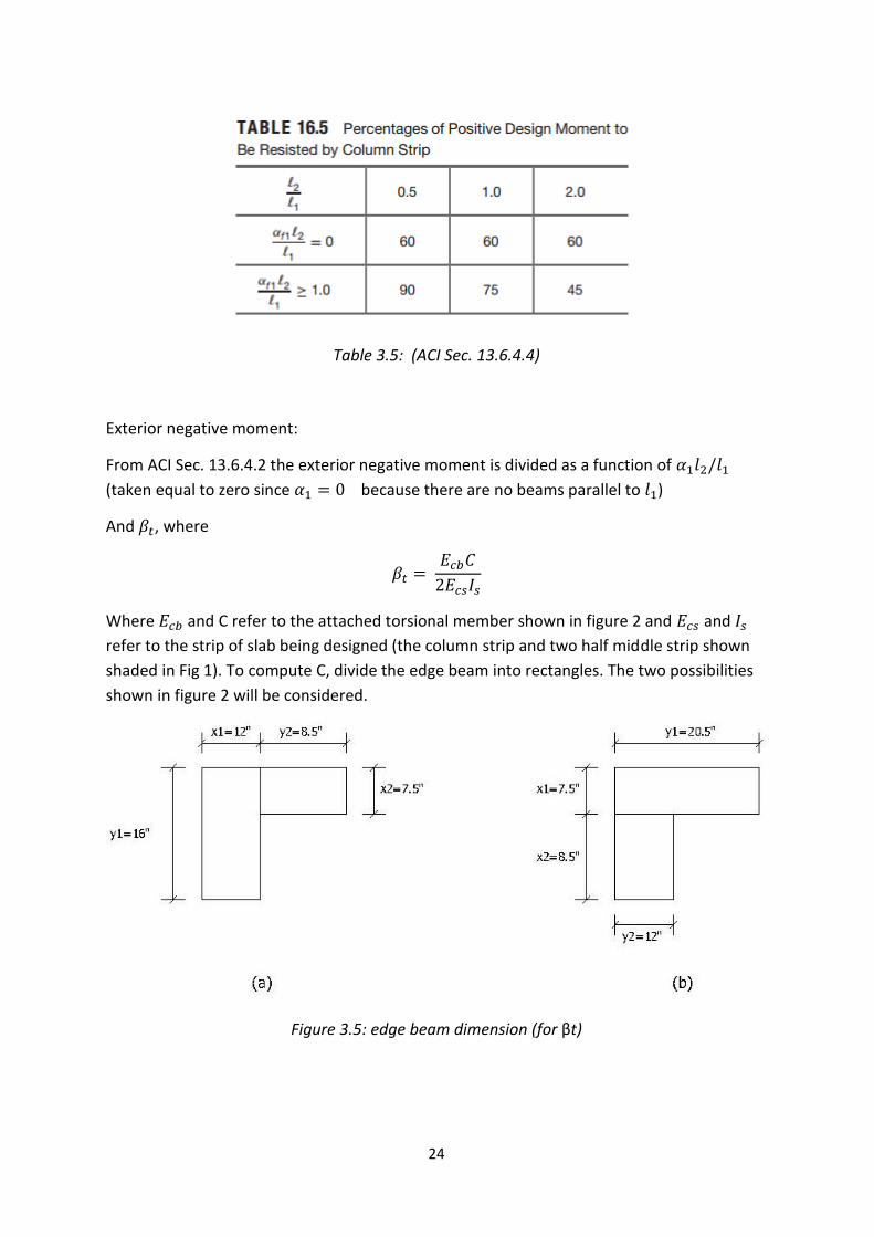
Positive Moments:
From ACI Sec. 13.6.4.4, where 𝛼1𝑙2/𝑙1 = 0
Column strip positive moment = 0.6 x 103.29 = 61.98 k-ft
Middle strip positive moment = 0.4 x 103.29 = 41.32 k-ft
24
Table 3.5: (ACI Sec. 13.6.4.4)
Exterior negative moment:
From ACI Sec. 13.6.4.2 the exterior negative moment is divided as a function of 𝛼1𝑙2/𝑙1
(taken equal to zero since 𝛼1 = 0 because there are no beams parallel to 𝑙1)
And 𝛽𝑡, where
𝛽𝑡 = 𝐸𝑐𝑏𝐶
2𝐸𝑐𝑠𝐼𝑠
Where 𝐸𝑐𝑏 and C refer to the attached torsional member shown in figure 2 and 𝐸𝑐𝑠 and 𝐼𝑠
refer to the strip of slab being designed (the column strip and two half middle strip shown
shaded in Fig 1). To compute C, divide the edge beam into rectangles. The two possibilities
shown in figure 2 will be considered.
Figure 3.5: edge beam dimension (for βt)
25
For figure 3, (ACI Eq. 13-7) gives
C = ∑⌈(1 − 0.63𝑥
𝑦)
𝑥3𝑦
3⌉
Where x= shorter length of the rectangle
y= longer length of the rectangle
For 3a,
C = (1−0.63×
12
16)×123×16)
3 +
(1−0.63×7.5
8.5)×7.53×8.5)
3 =5392.30𝑖𝑛4
For 3b,
C = (1−0.63×
7.5
20.5)×7.53×20.5)
3 +
(1−0.63×8.5
12)×8.53×12)
3 =3578.65𝑖𝑛4
The larger of these two values are used.
C= 5392.30𝑖𝑛4
𝐼𝑠 is the moment of inertia of the strip of slab being designed. It has b = 19ft and h=7.5 inch
𝐼𝑠 = (19×12)×7.53
12 = 8015.63 𝑖𝑛4
Since 𝑓𝑐′ is the same in the slab and beam, 𝐸𝑐𝑏= 𝐸𝑐𝑠 and 𝛽𝑡 =
5392.30
2∗8015.63 = 0.336
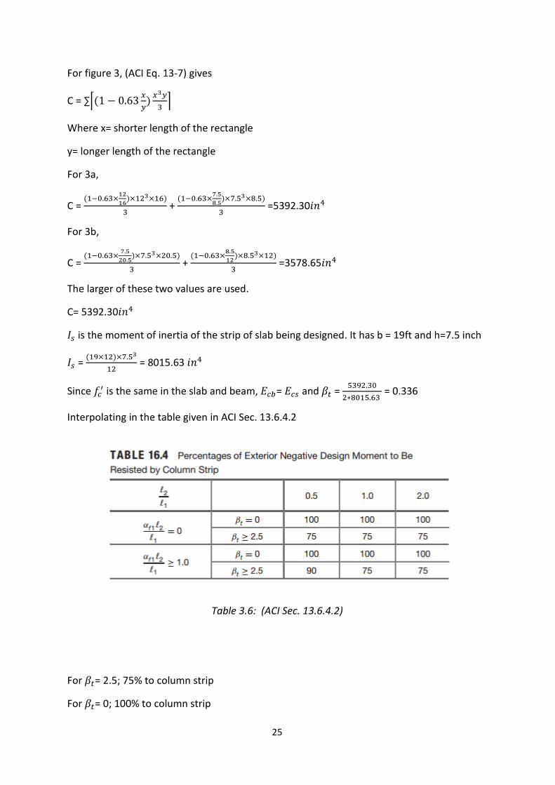
Interpolating in the table given in ACI Sec. 13.6.4.2
Table 3.6: (ACI Sec. 13.6.4.2)
For 𝛽𝑡= 2.5; 75% to column strip
For 𝛽𝑡= 0; 100% to column strip
26
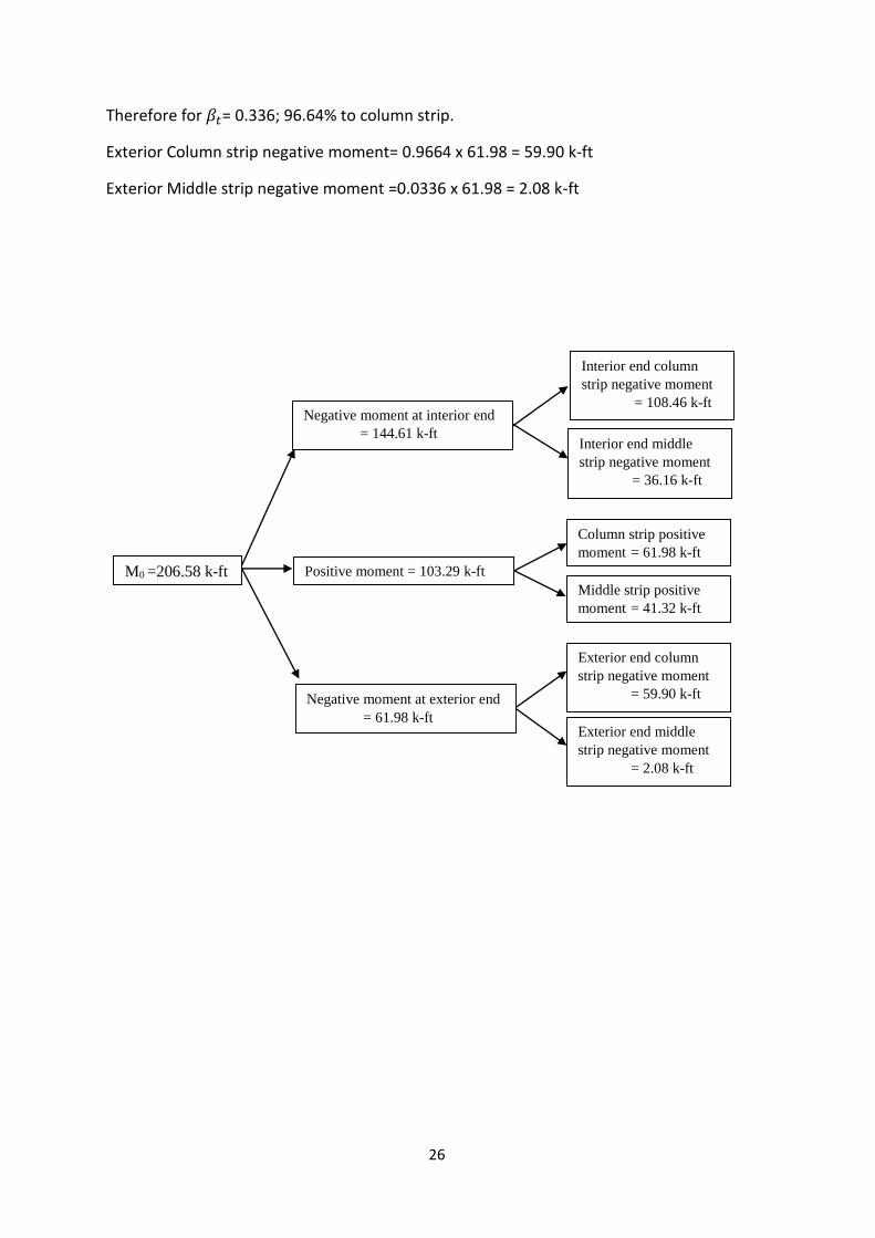
Therefore for 𝛽𝑡= 0.336; 96.64% to column strip.
Exterior Column strip negative moment= 0.9664 x 61.98 = 59.90 k-ft
Exterior Middle strip negative moment =0.0336 x 61.98 = 2.08 k-ft
M0 =206.58 k-ft
Negative moment at interior end
= 144.61 k-ft
Positive moment = 103.29 k-ft
Negative moment at exterior end
= 61.98 k-ft
Interior end column
strip negative moment
= 108.46 k-ft
Interior end middle
strip negative moment
= 36.16 k-ft
Column strip positive
moment = 61.98 k-ft
Middle strip positive
moment = 41.32 k-ft
Exterior end column
strip negative moment
= 59.90 k-ft
Exterior end middle
strip negative moment
= 2.08 k-ft
27
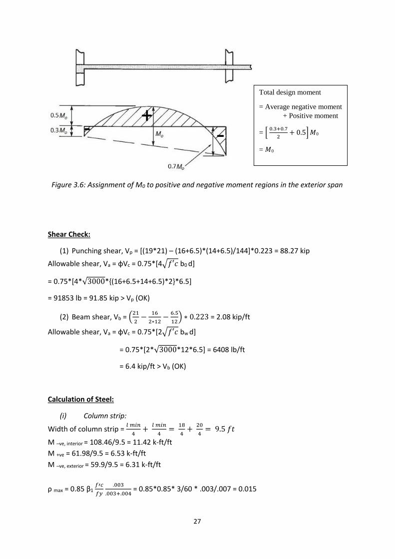
Figure 3.6: Assignment of M0 to positive and negative moment regions in the exterior span
Shear Check:
(1) Punching shear, Vp = [(19*21) – (16+6.5)*(14+6.5)/144]*0.223 = 88.27 kip
Allowable shear, Va = ɸVc = 0.75*[4√𝑓′𝑐 b0 d]
= 0.75*[4*√3000*{(16+6.5+14+6.5)*2}*6.5]
= 91853 lb = 91.85 kip > Vp (OK)
(2) Beam shear, Vb = (21
2−
16
2∗12−
6.5
12) ∗ 0.223 = 2.08 kip/ft
Allowable shear, Va = ɸVc = 0.75*[2√𝑓′𝑐 bw d]
= 0.75*[2*√3000*12*6.5] = 6408 lb/ft
= 6.4 kip/ft > Vb (OK)
Calculation of Steel:
(i) Column strip:
Width of column strip = 𝑙 𝑚𝑖𝑛
4+
𝑙 𝑚𝑖𝑛
4=
18
4+
20
4= 9.5 𝑓𝑡
M –ve, interior = 108.46/9.5 = 11.42 k-ft/ft
M +ve = 61.98/9.5 = 6.53 k-ft/ft
M –ve, exterior = 59.9/9.5 = 6.31 k-ft/ft
ρ max = 0.85 β1 𝑓′𝑐
𝑓𝑦
.003
.003+.004 = 0.85*0.85* 3/60 * .003/.007 = 0.015
Total design moment
= Average negative moment
+ Positive moment
= [ 0.3+0.7
2+ 0.5] 𝑀0
= 𝑀0
28
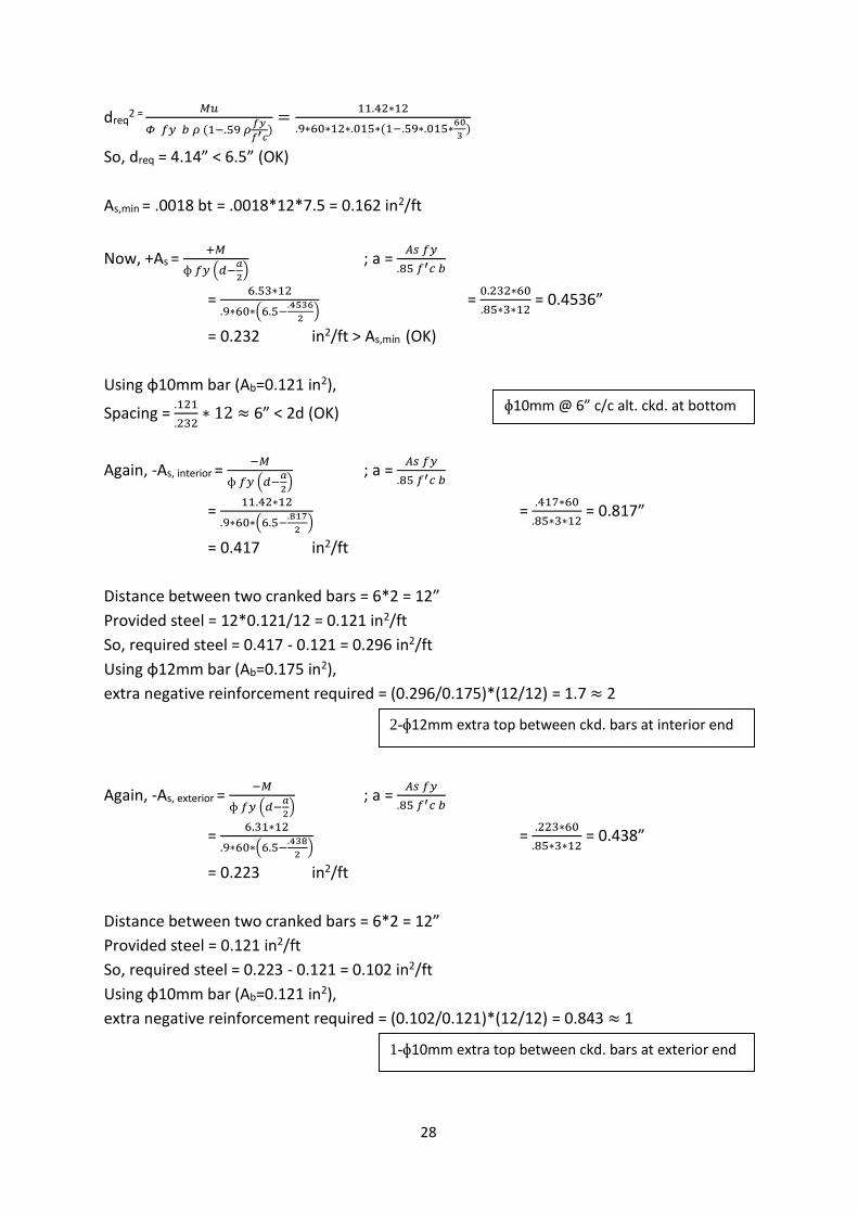
dreq2 = 𝑀𝑢
𝛷 𝑓𝑦 𝑏 𝜌 (1−.59 𝜌𝑓𝑦
𝑓′𝑐)
=11.42∗12
.9∗60∗12∗.015∗(1−.59∗.015∗60
3)
So, dreq = 4.14” < 6.5” (OK)
As,min = .0018 bt = .0018*12*7.5 = 0.162 in2/ft
Now, +As = +𝑀
ɸ 𝑓𝑦 (𝑑−𝑎
2) ; a =
𝐴𝑠 𝑓𝑦
.85 𝑓′𝑐 𝑏
= 6.53∗12
.9∗60∗(6.5−.4536
2) =
0.232∗60
.85∗3∗12 = 0.4536”
= 0.232 in2/ft > As,min (OK)
Using ɸ10mm bar (Ab=0.121 in2),
Spacing = .121
.232∗ 12 ≈ 6” < 2d (OK)
Again, -As, interior = −𝑀
ɸ 𝑓𝑦 (𝑑−𝑎
2) ; a =
𝐴𝑠 𝑓𝑦
.85 𝑓′𝑐 𝑏
= 11.42∗12
.9∗60∗(6.5−.817
2) =
.417∗60
.85∗3∗12 = 0.817”
= 0.417 in2/ft
Distance between two cranked bars = 6*2 = 12”
Provided steel = 12*0.121/12 = 0.121 in2/ft
So, required steel = 0.417 - 0.121 = 0.296 in2/ft
Using ɸ12mm bar (Ab=0.175 in2),
extra negative reinforcement required = (0.296/0.175)*(12/12) = 1.7 ≈ 2
Again, -As, exterior = −𝑀
ɸ 𝑓𝑦 (𝑑−𝑎
2) ; a =
𝐴𝑠 𝑓𝑦
.85 𝑓′𝑐 𝑏
= 6.31∗12
.9∗60∗(6.5−.438
2) =
.223∗60
.85∗3∗12 = 0.438”
= 0.223 in2/ft
Distance between two cranked bars = 6*2 = 12”
Provided steel = 0.121 in2/ft
So, required steel = 0.223 - 0.121 = 0.102 in2/ft
Using ɸ10mm bar (Ab=0.121 in2),
extra negative reinforcement required = (0.102/0.121)*(12/12) = 0.843 ≈ 1
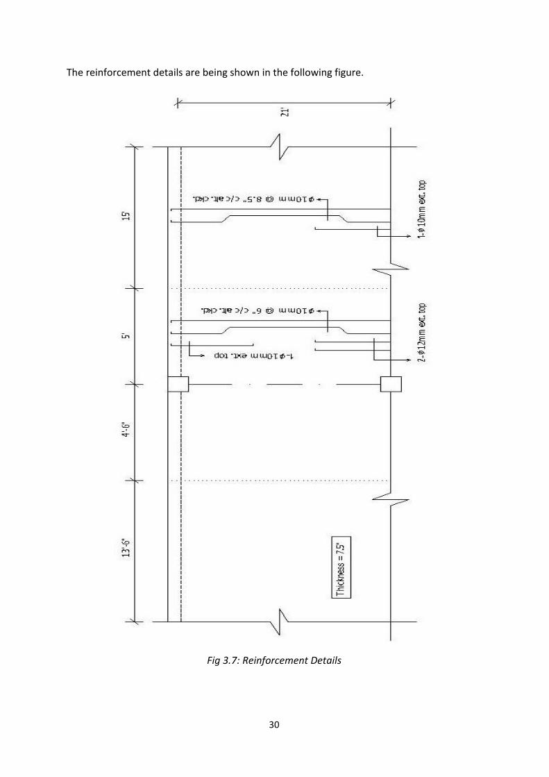
1-ɸ10mm extra top between ckd. bars at exterior end
ɸ10mm @ 6” c/c alt. ckd. at bottom
2-ɸ12mm extra top between ckd. bars at interior end
29
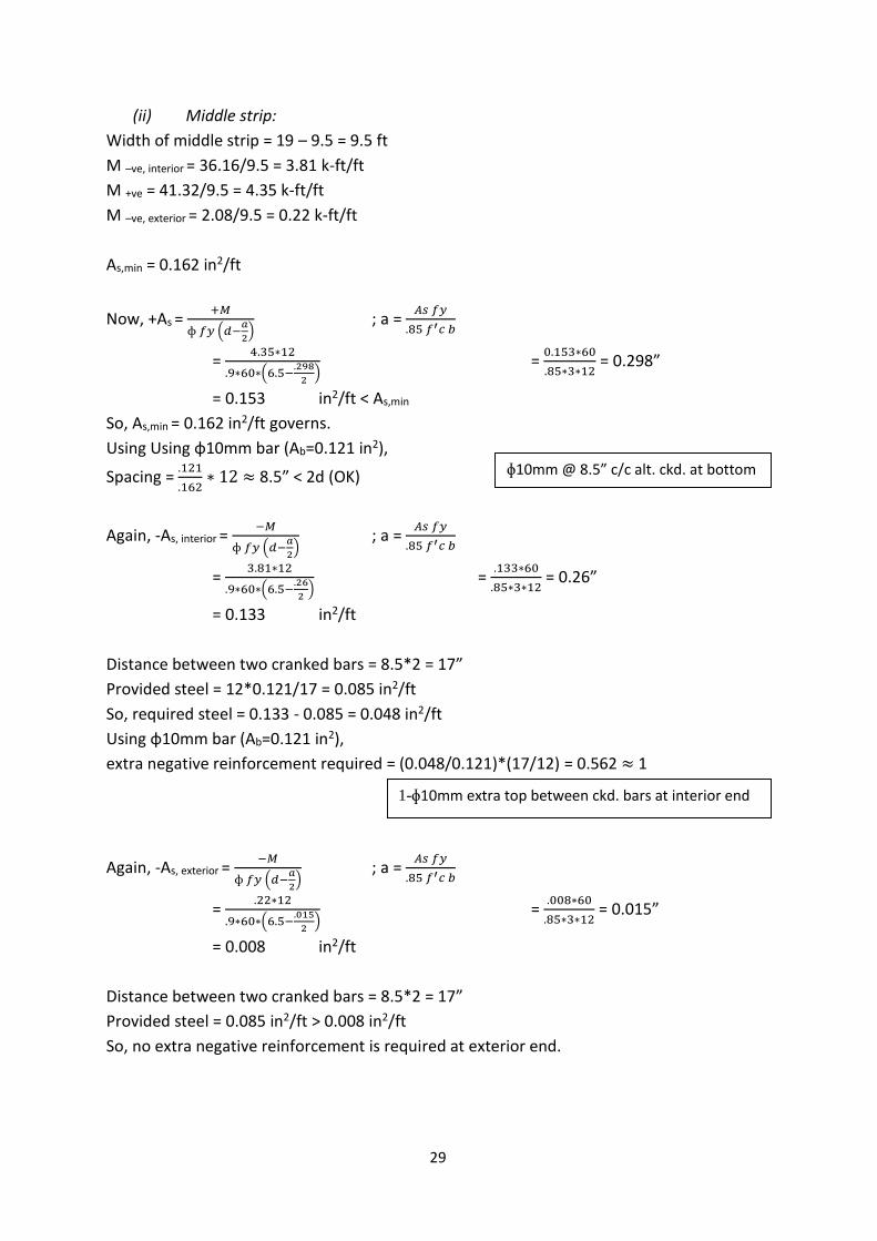
(ii) Middle strip:
Width of middle strip = 19 – 9.5 = 9.5 ft
M –ve, interior = 36.16/9.5 = 3.81 k-ft/ft
M +ve = 41.32/9.5 = 4.35 k-ft/ft
M –ve, exterior = 2.08/9.5 = 0.22 k-ft/ft
As,min = 0.162 in2/ft
Now, +As = +𝑀
ɸ 𝑓𝑦 (𝑑−𝑎
2) ; a =
𝐴𝑠 𝑓𝑦
.85 𝑓′𝑐 𝑏
= 4.35∗12
.9∗60∗(6.5−.298
2) =
0.153∗60
.85∗3∗12 = 0.298”
= 0.153 in2/ft < As,min
So, As,min = 0.162 in2/ft governs.
Using Using ɸ10mm bar (Ab=0.121 in2),
Spacing = .121
.162∗ 12 ≈ 8.5” < 2d (OK)
Again, -As, interior = −𝑀
ɸ 𝑓𝑦 (𝑑−𝑎
2) ; a =
𝐴𝑠 𝑓𝑦
.85 𝑓′𝑐 𝑏
= 3.81∗12
.9∗60∗(6.5−.26
2) =
.133∗60
.85∗3∗12 = 0.26”
= 0.133 in2/ft
Distance between two cranked bars = 8.5*2 = 17”
Provided steel = 12*0.121/17 = 0.085 in2/ft
So, required steel = 0.133 - 0.085 = 0.048 in2/ft
Using ɸ10mm bar (Ab=0.121 in2),
extra negative reinforcement required = (0.048/0.121)*(17/12) = 0.562 ≈ 1
Again, -As, exterior = −𝑀
ɸ 𝑓𝑦 (𝑑−𝑎
2) ; a =
𝐴𝑠 𝑓𝑦
.85 𝑓′𝑐 𝑏
= .22∗12
.9∗60∗(6.5−.015
2) =
.008∗60
.85∗3∗12 = 0.015”
= 0.008 in2/ft
Distance between two cranked bars = 8.5*2 = 17”
Provided steel = 0.085 in2/ft > 0.008 in2/ft
So, no extra negative reinforcement is required at exterior end.
ɸ10mm @ 8.5” c/c alt. ckd. at bottom
1-ɸ10mm extra top between ckd. bars at interior end
30
The reinforcement details are being shown in the following figure.
Fig 3.7: Reinforcement Details
31
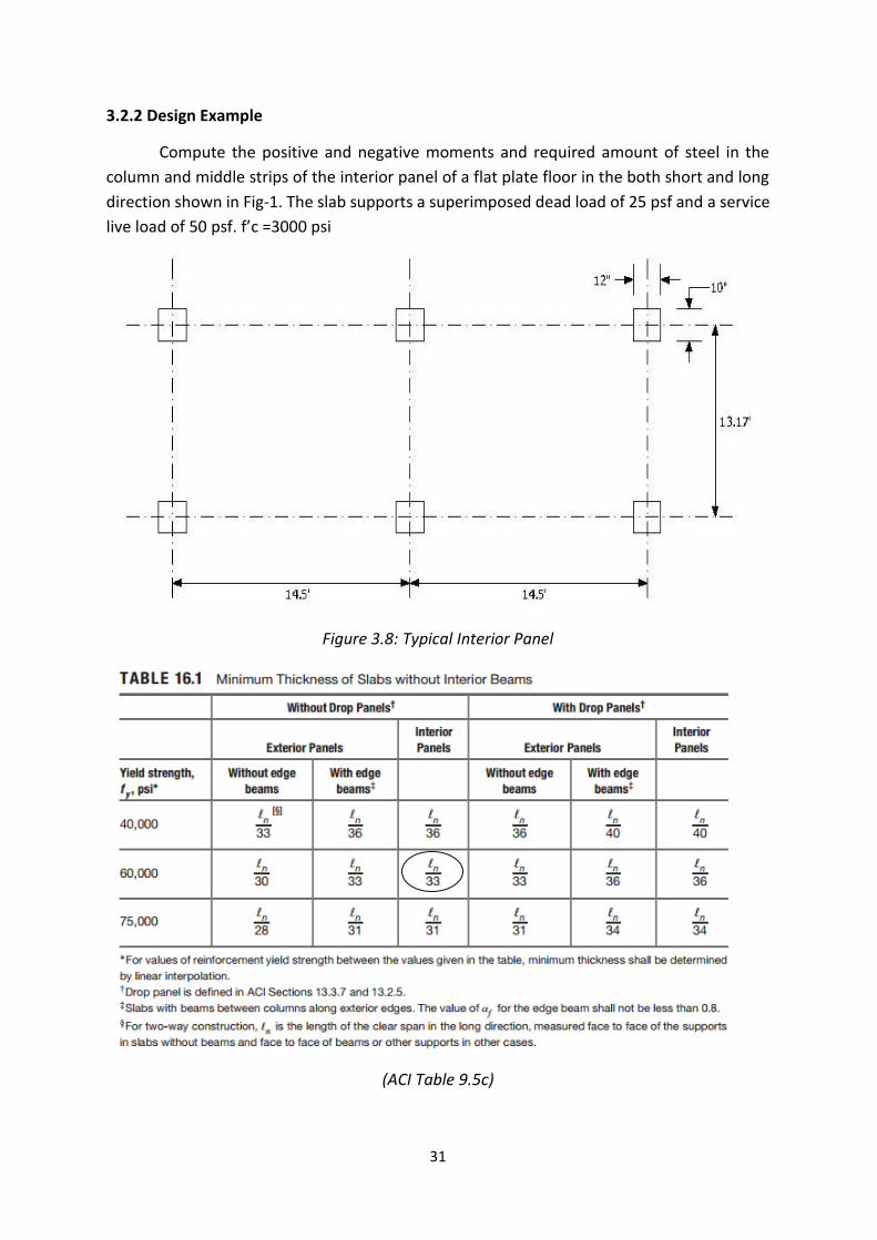
3.2.2 Design Example
Compute the positive and negative moments and required amount of steel in the
column and middle strips of the interior panel of a flat plate floor in the both short and long
direction shown in Fig-1. The slab supports a superimposed dead load of 25 psf and a service
live load of 50 psf. f’c =3000 psi
Figure 3.8: Typical Interior Panel
(ACI Table 9.5c)
32
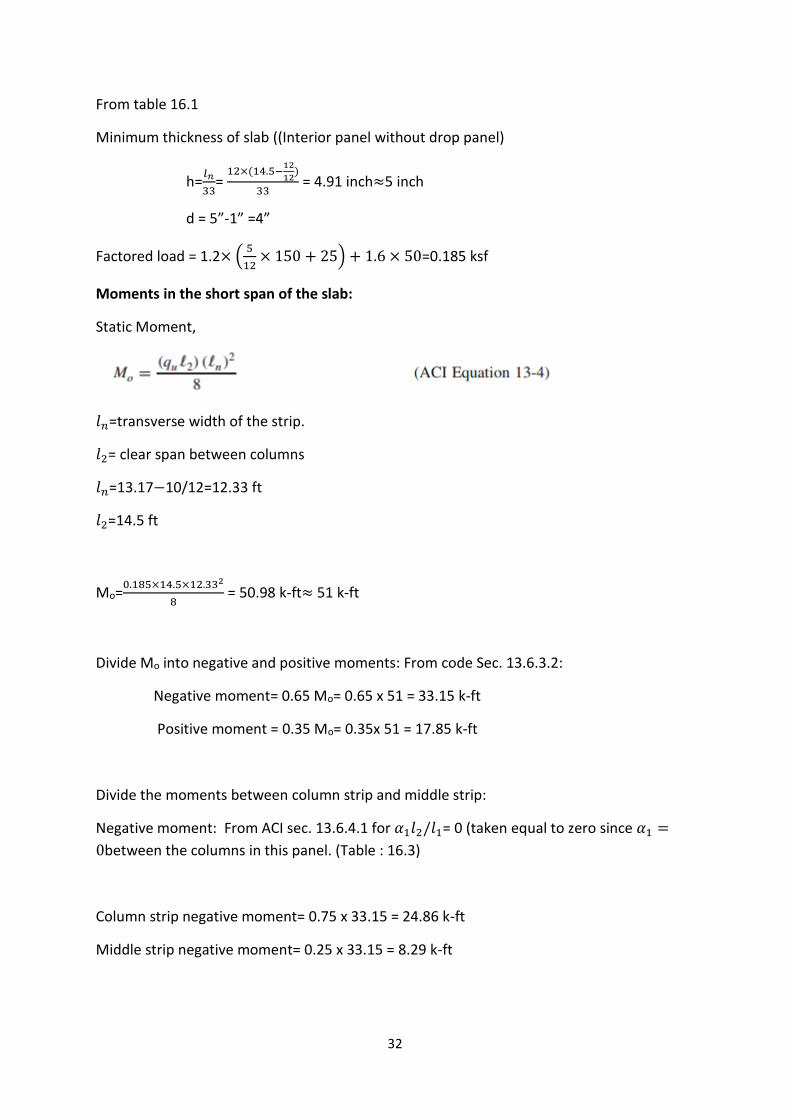
From table 16.1
Minimum thickness of slab ((Interior panel without drop panel)
h=𝑙𝑛
33=
12×(14.5−12
12)
33 = 4.91 inch≈5 inch
d = 5”-1” =4”
Factored load = 1.2× (5
12× 150 + 25) + 1.6 × 50=0.185 ksf
Moments in the short span of the slab:
Static Moment,
𝑙𝑛=transverse width of the strip.
𝑙2= clear span between columns
𝑙𝑛=13.17−10/12=12.33 ft
𝑙2=14.5 ft
Mo=0.185×14.5×12.332
8 = 50.98 k-ft≈ 51 k-ft
Divide Mo into negative and positive moments: From code Sec. 13.6.3.2:
Negative moment= 0.65 Mo= 0.65 x 51 = 33.15 k-ft
Positive moment = 0.35 Mo= 0.35x 51 = 17.85 k-ft
Divide the moments between column strip and middle strip:
Negative moment: From ACI sec. 13.6.4.1 for 𝛼1𝑙2/𝑙1= 0 (taken equal to zero since 𝛼1 =
0between the columns in this panel. (Table : 16.3)
Column strip negative moment= 0.75 x 33.15 = 24.86 k-ft
Middle strip negative moment= 0.25 x 33.15 = 8.29 k-ft
33
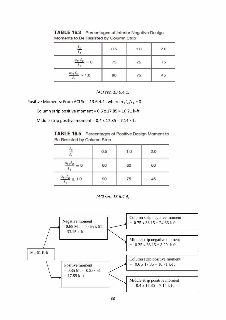
(ACI sec. 13.6.4.1)
Positive Moments: From ACI Sec. 13.6.4.4 , where 𝛼1𝑙2/𝑙1 = 0
Column strip positive moment = 0.6 x 17.85 = 10.71 k-ft
Middle strip positive moment = 0.4 x 17.85 = 7.14 k-ft
(ACI sec. 13.6.4.4)
Mo=51 K-ft
Negative moment
= 0.65 M o = 0.65 x 51
= 33.15 k-ft
Positive moment
= 0.35 Mo = 0.35x 51
= 17.85 k-ft
Column strip negative moment
= 0.75 x 33.15 = 24.86 k-ft
Middle strip negative moment
= 0.25 x 33.15 = 8.29 k-ft
Column strip positive moment
= 0.6 x 17.85 = 10.71 k-ft
Middle strip positive moment
= 0.4 x 17.85 = 7.14 k-ft
34
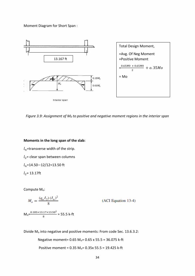
Moment Diagram for Short Span :
Figure 3.9: Assignment of M0 to positive and negative moment regions in the interior span
Moments in the long span of the slab:
𝑙𝑛=transverse width of the strip.
𝑙2= clear span between columns
𝑙𝑛=14.50−12/12=13.50 ft
𝑙2= 13.17ft
Compute Mo:
Mo=0.185×13.17×13.502
8 = 55.5 k-ft
Divide Mo into negative and positive moments: From code Sec. 13.6.3.2:
Negative moment= 0.65 Mo= 0.65 x 55.5 = 36.075 k-ft
Positive moment = 0.35 Mo= 0.35x 55.5 = 19.425 k-ft
13.167 ft
Total Design Moment,
=Avg. Of Neg Moment
+Positive Moment
=0.65𝑀0 + 0.65𝑀0
2 + 𝑜. 35𝑀𝑜
= Mo
35
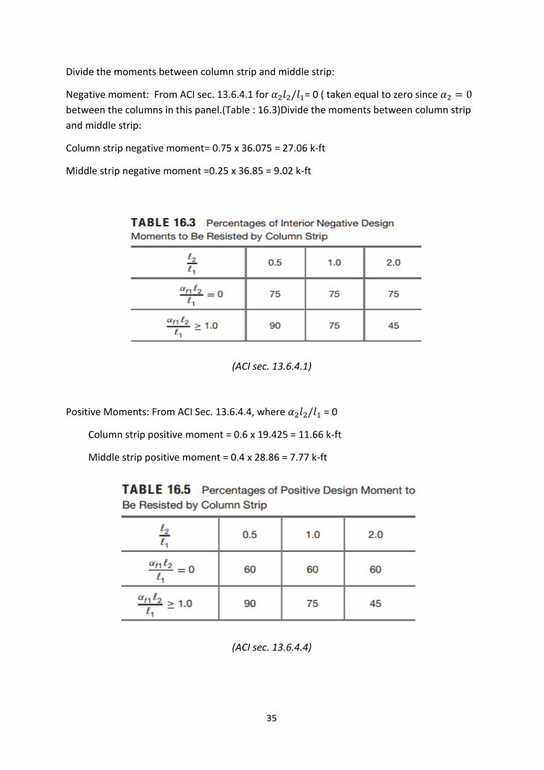
Divide the moments between column strip and middle strip:
Negative moment: From ACI sec. 13.6.4.1 for 𝛼2𝑙2/𝑙1= 0 ( taken equal to zero since 𝛼2 = 0
between the columns in this panel.(Table : 16.3)Divide the moments between column strip
and middle strip:
Column strip negative moment= 0.75 x 36.075 = 27.06 k-ft
Middle strip negative moment =0.25 x 36.85 = 9.02 k-ft
(ACI sec. 13.6.4.1)
Positive Moments: From ACI Sec. 13.6.4.4, where 𝛼2𝑙2/𝑙1 = 0
Column strip positive moment = 0.6 x 19.425 = 11.66 k-ft
Middle strip positive moment = 0.4 x 28.86 = 7.77 k-ft
(ACI sec. 13.6.4.4)
36
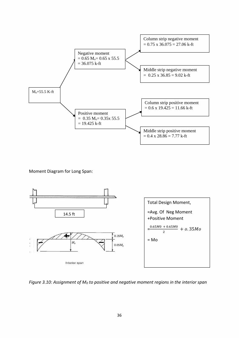
Moment Diagram for Long Span:
Figure 3.10: Assignment of M0 to positive and negative moment regions in the interior span
Mo=55.5 K-ft
Negative moment
= 0.65 Mo= 0.65 x 55.5
= 36.075 k-ft
Positive moment
= 0.35 Mo= 0.35x 55.5
= 19.425 k-ft
Middle strip negative moment
= 0.25 x 36.85 = 9.02 k-ft
Column strip negative moment
= 0.75 x 36.075 = 27.06 k-ft
Column strip positive moment
= 0.6 x 19.425 = 11.66 k-ft
Middle strip positive moment
= 0.4 x 28.86 = 7.77 k-ft
Total Design Moment,
=Avg. Of Neg Moment
+Positive Moment
=0.65𝑀0 + 0.65𝑀0
2 + 𝑜. 35𝑀𝑜
= Mo
14.5 ft
37
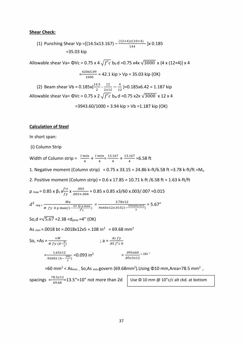
Shear Check:
(1) Punching Shear Vp =[(14.5x13.167) – (12+4)𝑥(10+4)
144 ]x 0.185
=35.03 kip
Allowable shear Va= ΦVc = 0.75 x 4 √𝑓′𝑐 b0 d =0.75 x4x √3000 x {4 x (12+4)} x 4
=42065.09
1000 = 42.1 kip > Vp = 35.03 kip (OK)
(2) Beam shear Vb = 0.185x(14.5
2 -
12
2𝑥12−
4
12 )=0.185x6.42 = 1.187 kip
Allowable shear Va= ΦVc = 0.75 x 2 √𝑓′𝑐 bw d =0.75 x2x √3000 x 12 x 4
=3943.60/1000 = 3.94 kip > Vb =1.187 kip (OK)
Calculation of Steel
In short span:
(i) Column Strip
Width of Column strip = 𝑙 𝑚𝑖𝑛
4+
𝑙 𝑚𝑖𝑛
4=
13.167
4+
13.167
4 =6.58 ft
1. Negative moment (Column strip) = 0.75 x 33.15 = 24.86 k-ft/6.58 ft =3.78 k-ft/ft =Mu
2. Positive moment (Column strip) = 0.6 x 17.85 = 10.71 k-ft /6.58 ft = 1.63 k-ft/ft
ρ max = 0.85 x β1 x𝑓′𝑐
𝑓𝑦 x
.003
.003+.004 = 0.85 x 0.85 x3/60 x.003/.007 =0.015
𝑑2 req = 𝑀𝑢
𝛷 𝑓𝑦 𝑏 ρ max(1−.59 fy ρ max
f′c) =
3.78𝑥12
.9𝑥60𝑥12𝑥.015(1−.59𝑥60𝑥.015
3) = 5.67”
So,d =√5.67 =2.38 <dprov =4” (OK)
As min =.0018 bt =.0018x12x5 =.108 in2 = 69.68 mm2
So, +As = +𝑀
𝛷 𝑓𝑦 (𝑑−𝑎
2) ; a =
𝐴𝑠 𝑓𝑦
.85 𝑓′𝑐 𝑏
=1.63𝑥12
.9𝑥60𝑥 (4− .181
2)
=0.093 in2 = .093𝑥60
.85𝑥3𝑥12 =.181 “
=60 mm2 < Asmin , So,As min govern (69.68mm2).Using Φ10 mm,Area=78.5 mm2 ,
spacings =78.5𝑥12
69.68=13.5“=10” not more than 2d
Use Φ 10 mm @ 10”c/c alt ckd. at bottom
38
Again. -As = −𝑀
𝛷 𝑓𝑦 (𝑑−𝑎
2) ; a =
𝐴𝑠 𝑓𝑦
.85 𝑓′𝑐 𝑏
=3.78𝑥12
.9𝑥60𝑥 (4− .435
2)
=0.22in2 = .22𝑥60
.85𝑥3𝑥12 = .435”
=143.23 mm2 > Asmin ,
So,using Φ12 mm , distance between ckd bars 10x2=20”
Provided Steel =12𝑥113
24 = 56.5 mm2; so required steel =143.23-56.5=86.73 mm2
Using 1Φ12 mm as extra top, area=1x113 =113 mm2 >86.73 mm2
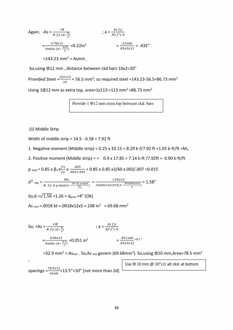
(ii) Middle Strip
Width of middle strip = 14.5 - 6.58 = 7.92 ft
1. Negative moment (Middle strip) = 0.25 x 33.15 = 8.29 k-f/7.92 ft =1.05 k-ft/ft =Mu
2. Positive moment (Middle strip) = = 0.4 x 17.85 = 7.14 k-ft /7.92ft = 0.90 k-ft/ft
ρ max = 0.85 x β1 x𝑓′𝑐
𝑓𝑦 x
.003
.003+.004 = 0.85 x 0.85 x3/60 x.003/.007 =0.015
𝑑2 req = 𝑀𝑢
𝛷 𝑓𝑦 𝑏 ρ max(1−.59 fy ρ max
f′c) =
1.05𝑥12
.9𝑥60𝑥12𝑥.015(1−.59𝑥60𝑥.015
3) = 1.58”
So,d =√1.58 =1.26 < dprov =4” (OK)
As min =.0018 bt =.0018x12x5 =.108 in2 = 69.68 mm2
So, +As = +𝑀
𝛷 𝑓𝑦 (𝑑−𝑎
2) ; a =
𝐴𝑠 𝑓𝑦
.85 𝑓′𝑐 𝑏
=0.90𝑥12
.9𝑥60𝑥 (4− 0.1
2)
=0.051 in2 = .051𝑥60
.85𝑥3𝑥12 =0.1 “
=32.9 mm2 < Asmin , So,As min govern (69.68mm2). So,using Φ10 mm,Area=78.5 mm2
,
spacings =78.5𝑥12
69.68=13.5“=10” [not more than 2d]
Provide 1 Φ12 mm extra top between ckd. bars
Use Φ 10 mm @ 10”c/c alt ckd. at bottom
39
Again. -As = −𝑀
𝛷 𝑓𝑦 (𝑑−𝑎
2) ; a =
𝐴𝑠 𝑓𝑦
.85 𝑓′𝑐 𝑏
=1.05𝑥12
.9𝑥60𝑥 (4− 0.12
2)
=0.06in2 = .06𝑥60
.85𝑥3𝑥12 = 0.12”
=38.71 mm2 < Asmin , So,As min govern (69.68mm2).Using Φ10 mm,Area=78.5 mm2
spacings =78.5𝑥12
69.68=13.5“=10” [not more than 2d]
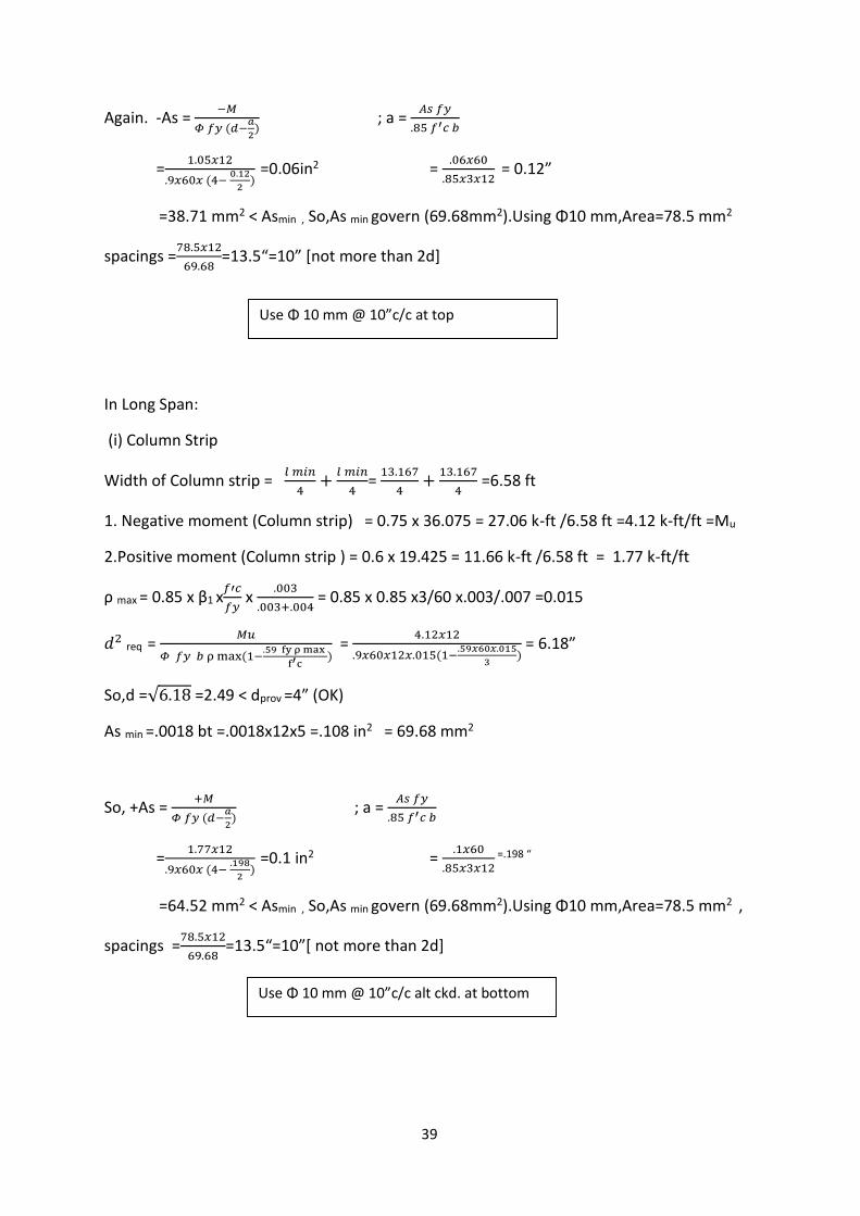
In Long Span:
(i) Column Strip
Width of Column strip = 𝑙 𝑚𝑖𝑛
4+
𝑙 𝑚𝑖𝑛
4=
13.167
4+
13.167
4 =6.58 ft
1. Negative moment (Column strip) = 0.75 x 36.075 = 27.06 k-ft /6.58 ft =4.12 k-ft/ft =Mu
2.Positive moment (Column strip ) = 0.6 x 19.425 = 11.66 k-ft /6.58 ft = 1.77 k-ft/ft
ρ max = 0.85 x β1 x𝑓′𝑐
𝑓𝑦 x
.003
.003+.004 = 0.85 x 0.85 x3/60 x.003/.007 =0.015
𝑑2 req = 𝑀𝑢
𝛷 𝑓𝑦 𝑏 ρ max(1−.59 fy ρ max
f′c) =
4.12𝑥12
.9𝑥60𝑥12𝑥.015(1−.59𝑥60𝑥.015
3) = 6.18”
So,d =√6.18 =2.49 < dprov =4” (OK)
As min =.0018 bt =.0018x12x5 =.108 in2 = 69.68 mm2
So, +As = +𝑀
𝛷 𝑓𝑦 (𝑑−𝑎
2) ; a =
𝐴𝑠 𝑓𝑦
.85 𝑓′𝑐 𝑏
=1.77𝑥12
.9𝑥60𝑥 (4− .198
2)
=0.1 in2 = .1𝑥60
.85𝑥3𝑥12 =.198 “
=64.52 mm2 < Asmin , So,As min govern (69.68mm2).Using Φ10 mm,Area=78.5 mm2 ,
spacings =78.5𝑥12
69.68=13.5“=10”[ not more than 2d]
Use Φ 10 mm @ 10”c/c at top
Use Φ 10 mm @ 10”c/c alt ckd. at bottom
40
Again. -As = −𝑀
𝛷 𝑓𝑦 (𝑑−𝑎
2) ; a =
𝐴𝑠 𝑓𝑦
.85 𝑓′𝑐 𝑏
=4.12𝑥12
.9𝑥60𝑥 (4− .48
2)
=0.24in2 = .24𝑥60
.85𝑥3𝑥12 = .48”
=154.84 mm2 > Asmin ,
So,using Φ12 mm , distance between ckd bars 10x2=20”
Provided Steel =12𝑥113
24 = 56.5 mm2 ;So. required steel =154.84 -56.5=98.34 mm2
Using 1Φ12 mm as extra top ,area=1x113 =113 mm2 >98.34 mm2
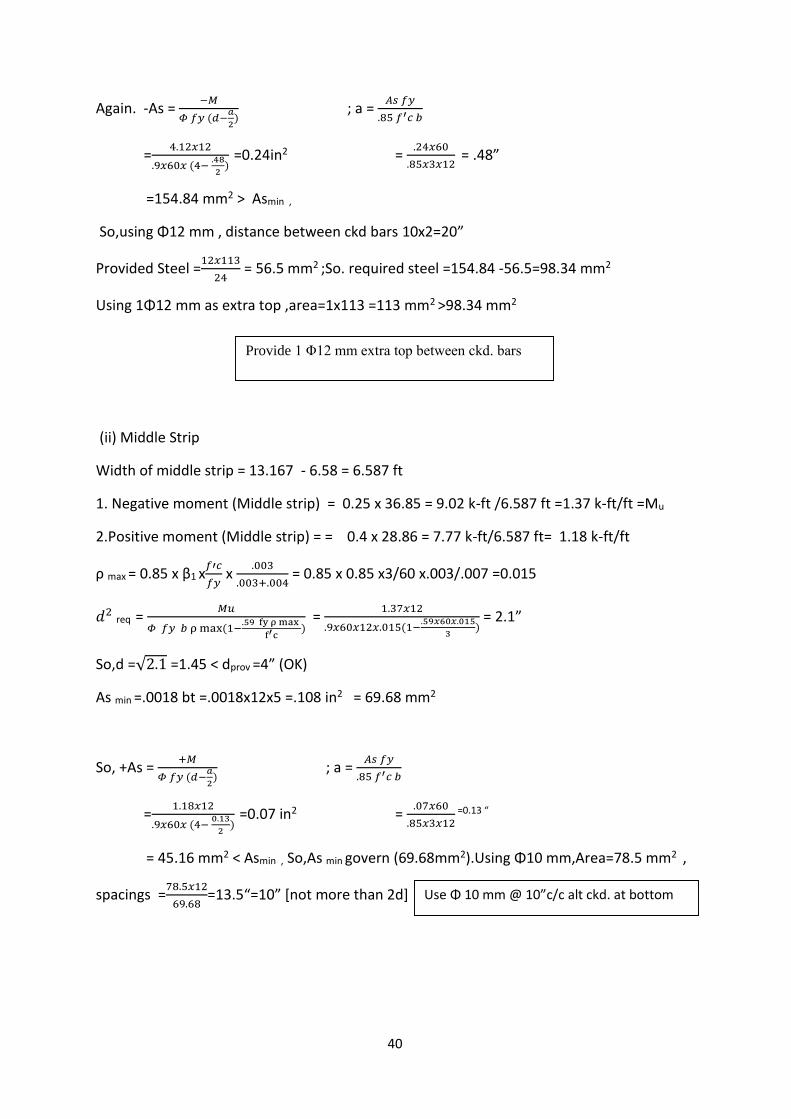
(ii) Middle Strip
Width of middle strip = 13.167 - 6.58 = 6.587 ft
1. Negative moment (Middle strip) = 0.25 x 36.85 = 9.02 k-ft /6.587 ft =1.37 k-ft/ft =Mu
2.Positive moment (Middle strip) = = 0.4 x 28.86 = 7.77 k-ft/6.587 ft= 1.18 k-ft/ft
ρ max = 0.85 x β1 x𝑓′𝑐
𝑓𝑦 x
.003
.003+.004 = 0.85 x 0.85 x3/60 x.003/.007 =0.015
𝑑2 req = 𝑀𝑢
𝛷 𝑓𝑦 𝑏 ρ max(1−.59 fy ρ max
f′c) =
1.37𝑥12
.9𝑥60𝑥12𝑥.015(1−.59𝑥60𝑥.015
3) = 2.1”
So,d =√2.1 =1.45 < dprov =4” (OK)
As min =.0018 bt =.0018x12x5 =.108 in2 = 69.68 mm2
So, +As = +𝑀
𝛷 𝑓𝑦 (𝑑−𝑎
2) ; a =
𝐴𝑠 𝑓𝑦
.85 𝑓′𝑐 𝑏
=1.18𝑥12
.9𝑥60𝑥 (4− 0.13
2)
=0.07 in2 = .07𝑥60
.85𝑥3𝑥12 =0.13 “
= 45.16 mm2 < Asmin , So,As min govern (69.68mm2).Using Φ10 mm,Area=78.5 mm2 ,
spacings =78.5𝑥12
69.68=13.5“=10” [not more than 2d]
Provide 1 Φ12 mm extra top between ckd. bars
Use Φ 10 mm @ 10”c/c alt ckd. at bottom
41
Again. -As = −𝑀
𝛷 𝑓𝑦 (𝑑−𝑎
2) ; a =
𝐴𝑠 𝑓𝑦
.85 𝑓′𝑐 𝑏
=1.37𝑥12
.9𝑥60𝑥 (4− 0.152
2)
=0.08in2 = .08𝑥60
.85𝑥3𝑥12 = 0.152”
=51.61 mm2 < Asmin , So,As min govern (69.68mm2) ,Using Φ10 mm,Area=78.5 mm2 ,
spacings =78.5𝑥12
69.68=13.5“=10” [not more than 2d]
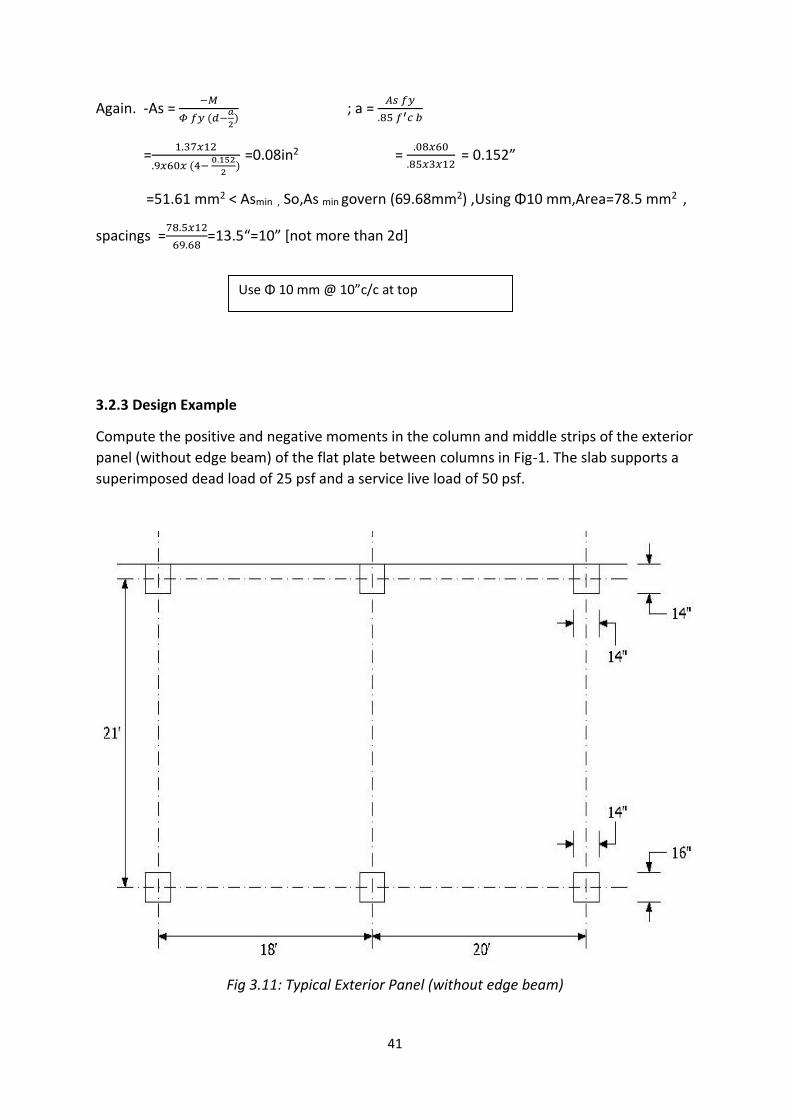
3.2.3 Design Example
Compute the positive and negative moments in the column and middle strips of the exterior
panel (without edge beam) of the flat plate between columns in Fig-1. The slab supports a
superimposed dead load of 25 psf and a service live load of 50 psf.
Fig 3.11: Typical Exterior Panel (without edge beam)
Use Φ 10 mm @ 10”c/c at top
42
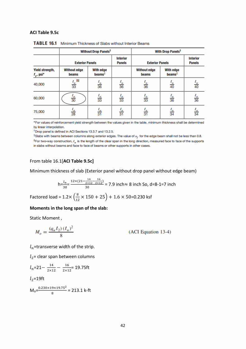
ACI Table 9.5c
From table 16.1[ACI Table 9.5c]
Minimum thickness of slab (Exterior panel without drop panel without edge beam)
h=𝑙𝑛
30=
12×(21−14
2×12−
16
2×12)
30 = 7.9 inch≈ 8 inch So, d=8-1=7 inch
Factored load = 1.2× (8
12× 150 + 25) + 1.6 × 50=0.230 ksf
Moments in the long span of the slab:
Static Moment ,
𝑙𝑛=transverse width of the strip.
𝑙2= clear span between columns
𝑙𝑛=21− 14
2×12−
16
2×12= 19.75ft
𝑙2=19ft
Mo=0.230×19×19.752
8 = 213.1 k-ft
43
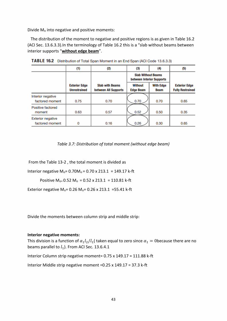
Divide Mo into negative and positive moments:
The distribution of the moment to negative and positive regions is as given in Table 16.2
(ACI Sec. 13.6.3.3).In the terminology of Table 16.2 this is a “slab without beams between
interior supports “without edge beam”.
Table 3.7: Distribution of total moment (without edge beam)
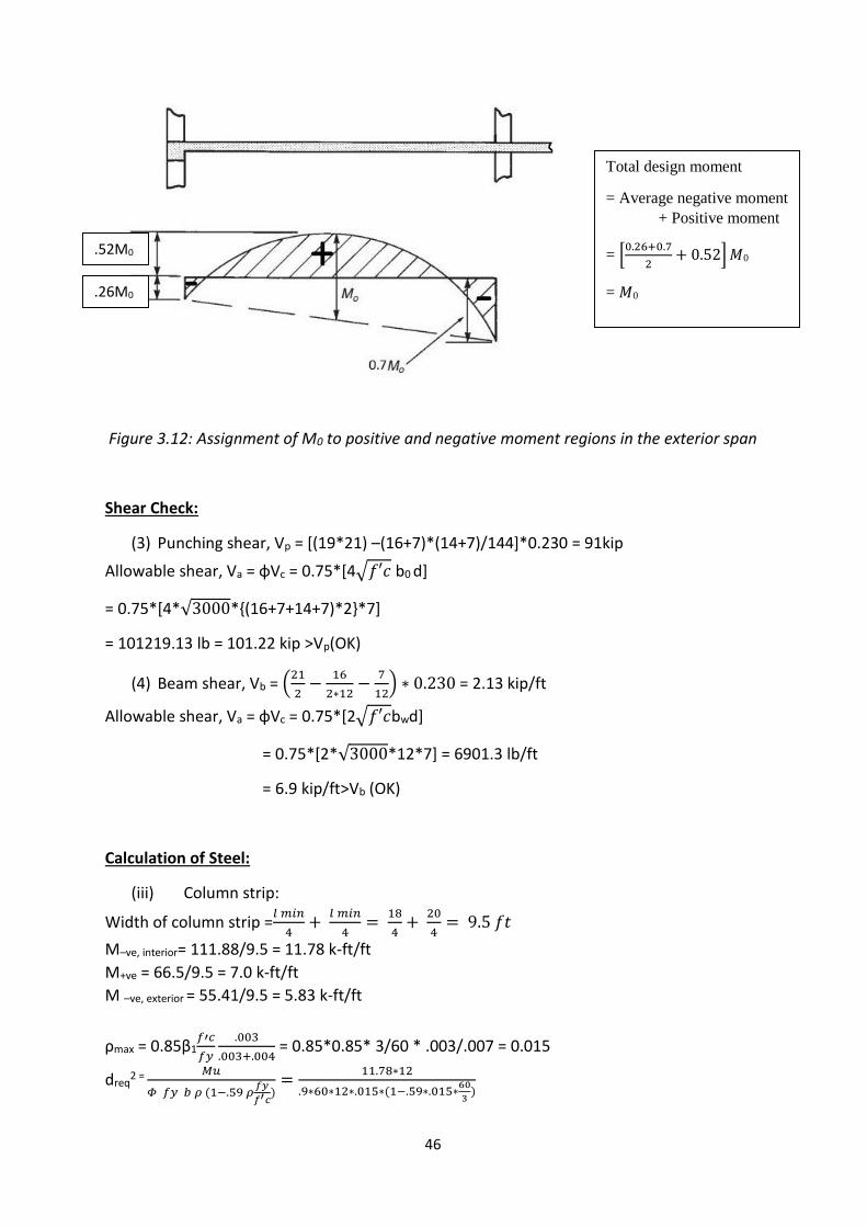
From the Table 13-2 , the total moment is divided as
Interior negative Mo= 0.70Mo = 0.70 x 213.1 = 149.17 k-ft
Positive Mo= 0.52 Mo = 0.52 x 213.1 = 110.81 k-ft
Exterior negative Mo= 0.26 Mo= 0.26 x 213.1 =55.41 k-ft
Divide the moments between column strip and middle strip:
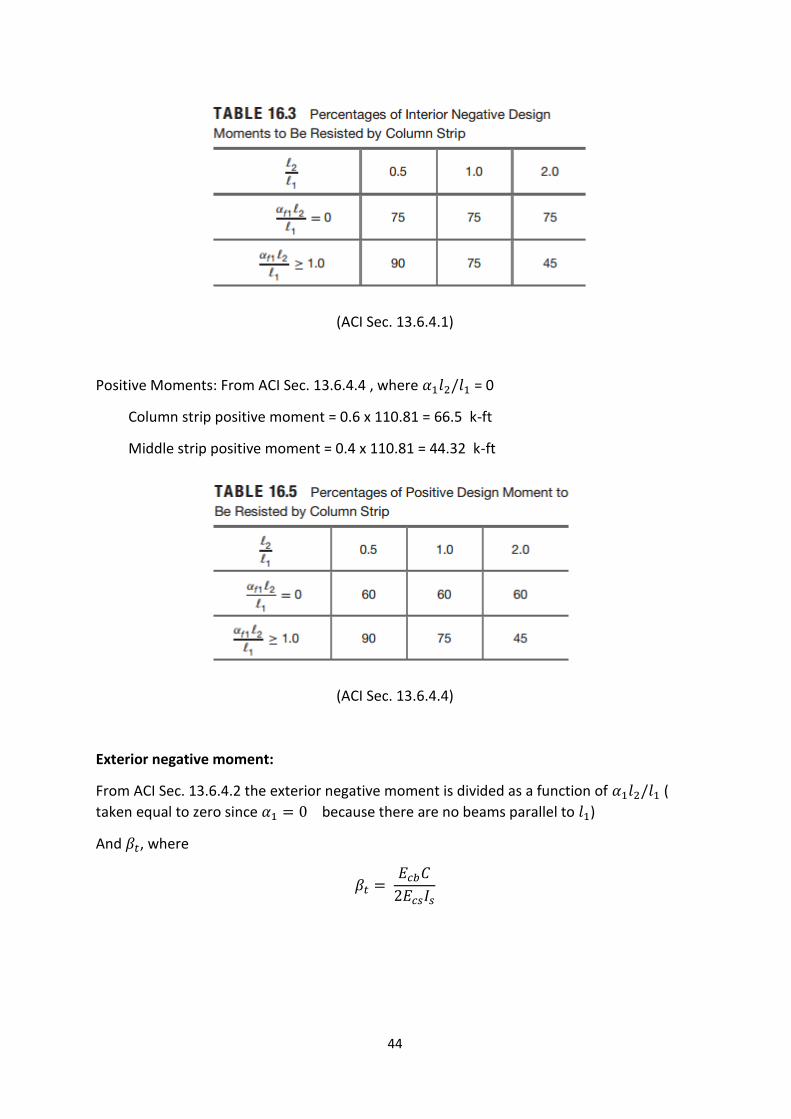
Interior negative moments:
This division is a function of 𝛼1𝑙2/𝑙1( taken equal to zero since 𝛼1 = 0because there are no
beams parallel to 𝑙1). From ACI Sec. 13.6.4.1
Interior Column strip negative moment= 0.75 x 149.17 = 111.88 k-ft
Interior Middle strip negative moment =0.25 x 149.17 = 37.3 k-ft
44
(ACI Sec. 13.6.4.1)
Positive Moments: From ACI Sec. 13.6.4.4 , where 𝛼1𝑙2/𝑙1 = 0
Column strip positive moment = 0.6 x 110.81 = 66.5 k-ft
Middle strip positive moment = 0.4 x 110.81 = 44.32 k-ft
(ACI Sec. 13.6.4.4)
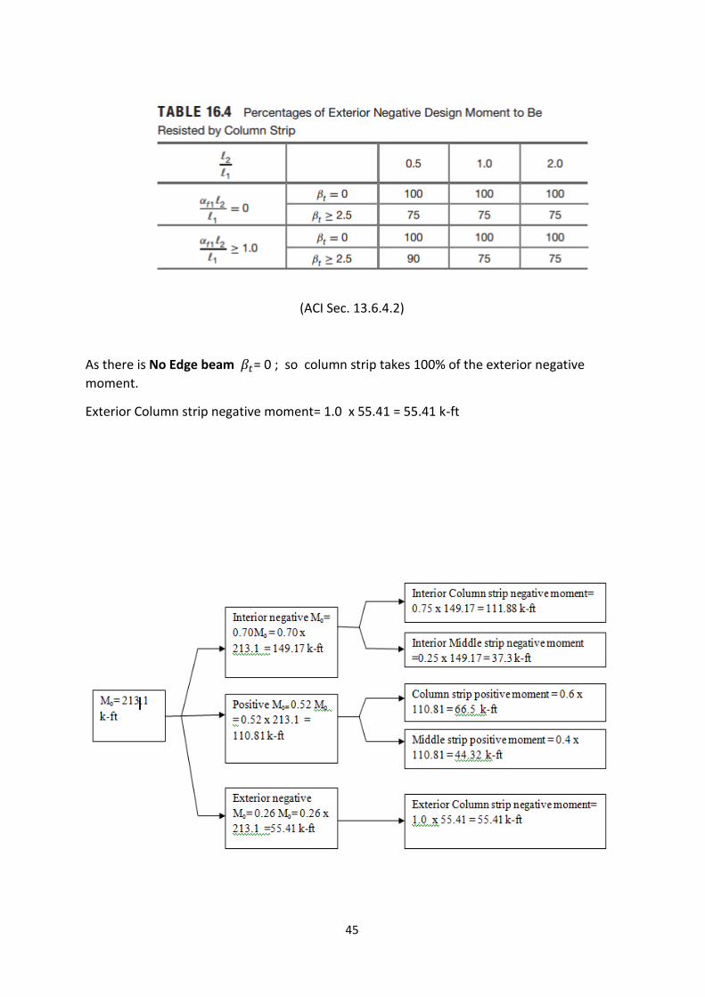
Exterior negative moment:
From ACI Sec. 13.6.4.2 the exterior negative moment is divided as a function of 𝛼1𝑙2/𝑙1 (
taken equal to zero since 𝛼1 = 0 because there are no beams parallel to 𝑙1)
And 𝛽𝑡, where
𝛽𝑡 = 𝐸𝑐𝑏𝐶
2𝐸𝑐𝑠𝐼𝑠
45
(ACI Sec. 13.6.4.2)
As there is No Edge beam 𝛽𝑡= 0 ; so column strip takes 100% of the exterior negative
moment.
Exterior Column strip negative moment= 1.0 x 55.41 = 55.41 k-ft
46
Figure 3.12: Assignment of M0 to positive and negative moment regions in the exterior span
Shear Check:
(3) Punching shear, Vp = [(19*21) –(16+7)*(14+7)/144]*0.230 = 91kip
Allowable shear, Va = ɸVc = 0.75*[4√𝑓′𝑐 b0 d]
= 0.75*[4*√3000*{(16+7+14+7)*2}*7]
= 101219.13 lb = 101.22 kip >Vp(OK)
(4) Beam shear, Vb = (21
2−
16
2∗12−
7
12) ∗ 0.230 = 2.13 kip/ft
Allowable shear, Va = ɸVc = 0.75*[2√𝑓′𝑐bwd]
= 0.75*[2*√3000*12*7] = 6901.3 lb/ft
= 6.9 kip/ft>Vb (OK)
Calculation of Steel:
(iii) Column strip:
Width of column strip =𝑙 𝑚𝑖𝑛
4+
𝑙 𝑚𝑖𝑛
4=
18
4+
20
4= 9.5 𝑓𝑡
M–ve, interior= 111.88/9.5 = 11.78 k-ft/ft
M+ve = 66.5/9.5 = 7.0 k-ft/ft
M –ve, exterior = 55.41/9.5 = 5.83 k-ft/ft
ρmax = 0.85β1𝑓′𝑐
𝑓𝑦
.003
.003+.004 = 0.85*0.85* 3/60 * .003/.007 = 0.015
dreq2 = 𝑀𝑢
𝛷 𝑓𝑦 𝑏 𝜌 (1−.59 𝜌𝑓𝑦
𝑓′𝑐)
=11.78∗12
.9∗60∗12∗.015∗(1−.59∗.015∗60
3)
Total design moment
= Average negative moment
+ Positive moment
= [0.26+0.7
2+ 0.52] 𝑀0
= 𝑀0
.52M0
.26M0
47
So, dreq = 4.20” < 7” (OK)
As,min= .0018 bt = .0018*12*8 = 0.173 in2/ft =111.61 mm2
Now, +As = +𝑀
ɸ 𝑓𝑦 (𝑑−𝑎
2) ; a =
𝐴𝑠 𝑓𝑦
.85 𝑓′𝑐 𝑏
=7∗12
.9∗60∗(7−.45
2) =
0.23∗60
.85∗3∗12 = 0.45”
= 0.230 in2/ft = 148.13 mm2 >As,min(OK)
Using Φ10 mm,Area=78.5 mm2 , spacings =78.5𝑥12
148.13=6.35“=6 ”[ not more than 2d] (OK)
Again, -As, interior= −𝑀
ɸ 𝑓𝑦 (𝑑−𝑎
2) ; a =
𝐴𝑠 𝑓𝑦
.85 𝑓′𝑐 𝑏
= 11.78∗12
.9∗60∗(6.5−.78
2) =
.417∗60
.85∗3∗12 = 0.78”
= 0.40 in2/ft =258.064 mm2
So,using Φ10 mm , distance between ckd bars 6x2=12”
Provided Steel =12𝑥78.5
12 = 78.5 mm2 ;So. required steel =258.064-78.5=179.56 mm2
Using 3Φ10 mm as extra top ,area=3x78.5 =235.5 mm2 >179.56mm2
Again, -As, exterior = −𝑀
ɸ 𝑓𝑦 (𝑑−𝑎
2) ; a =
𝐴𝑠 𝑓𝑦
.85 𝑓′𝑐 𝑏
= 5.83∗12
.9∗60∗(6.5−.373
2) =
..19∗60
.85∗3∗12 = 0.373”
= 0.19 in2/ft=122.58 mm2 >As,min(OK)
So,using Φ10 mm , distance between ckd bars 6x2=12”
Provided Steel =12𝑥78.5
12 = 78.5 mm2 ;So. required steel =122.58-78.5=44.08 mm2
Using 1Φ10 mm as extra top ,area=1x78.5 =78.5 mm2 >44.08mm2
(iv) Middle strip:
Width of middle strip = 20/2+18/2– 9.5 = 9.5 ft
M –ve, interior = 37.3/9.5 = 3.93 k-ft/ft
ɸ10mm @ 6” c/c alt. ckd. at bottom
3-ɸ10mm extra top betweenckd. bars at interior end
1-ɸ10mm extra top between ckd. Bars at exterior end
48
M +ve = 44.32/9.5 = 4.67 k-ft/ft
As,min = .0018 bt = .0018*12*8 = 0.173 in2/ft =111.61 mm2
Now, +As = +𝑀
ɸ 𝑓𝑦 (𝑑−𝑎
2) ; a =
𝐴𝑠 𝑓𝑦
.85 𝑓′𝑐 𝑏
= 4.67∗12
.9∗60∗(6.5−.297
2) =
0.151∗60
.85∗3∗12 = 0.297”
= 0.151 in2/ft =97.42mm2 <As,min
So, As,min= 111.61 mm2 governs.
Using Φ10 mm,Area=78.5 mm2 , spacings =78.5𝑥12
111.61=8.44= 8”[ not more than 2d] (OK)
Again, -As, interior = −𝑀
ɸ 𝑓𝑦 (𝑑−𝑎
2) ; a =
𝐴𝑠 𝑓𝑦
.85 𝑓′𝑐 𝑏
= 3.93∗12
.9∗60∗(6.5−.25
2) =
.13∗60
.85∗3∗12 = 0.25”
= 0.13 in2/ft =83.87 mm2
Distance between two cranked bars = 8*2 = 16”
Provided Steel =12𝑥78.5
16 = 58.87 mm2 ;So. required steel =83.87-58.87=25 mm2
Using 1Φ10 mm as extra top ,area=1x78.5 =78.5 mm2 >25mm2
ɸ10mm @ 8” c/c alt. ckd. at bottom
1-ɸ10mm extra top between ckd. bars at interior end
49
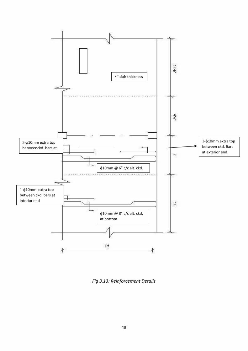
Fig 3.13: Reinforcement Details
ɸ10mm @ 6” c/c alt. ckd.
at bottom
3-ɸ10mm extra top
betweenckd. bars at
interior end
1-ɸ10mm extra top
between ckd. Bars
at exterior end
8” slab thickness
ɸ10mm @ 8” c/c alt. ckd.
at bottom
1-ɸ10mm extra top
between ckd. bars at
interior end
50
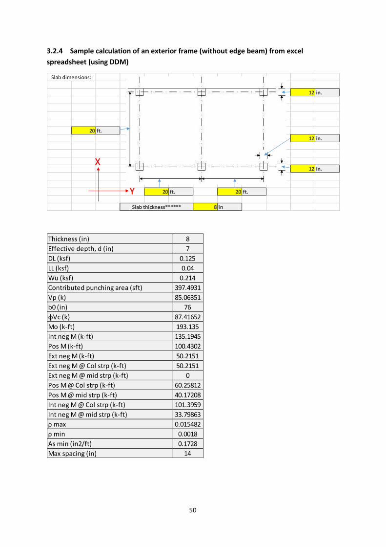
3.2.4 Sample calculation of an exterior frame (without edge beam) from excel
spreadsheet (using DDM)
12 in.
20 ft.
12 in.
12 in.
20 ft. 20 ft.
8 in
Slab dimensions:
Slab thickness******
X
Y
Thickness (in) 8
Effective depth, d (in) 7
DL (ksf) 0.125
LL (ksf) 0.04
Wu (ksf) 0.214
Contributed punching area (sft) 397.4931
Vp (k) 85.06351
b0 (in) 76
φVc (k) 87.41652
Mo (k-ft) 193.135
Int neg M (k-ft) 135.1945
Pos M (k-ft) 100.4302
Ext neg M (k-ft) 50.2151
Ext neg M @ Col strp (k-ft) 50.2151
Ext neg M @ mid strp (k-ft) 0
Pos M @ Col strp (k-ft) 60.25812
Pos M @ mid strp (k-ft) 40.17208
Int neg M @ Col strp (k-ft) 101.3959
Int neg M @ mid strp (k-ft) 33.79863
ρ max 0.015482
ρ min 0.0018
As min (in2/ft) 0.1728
Max spacing (in) 14
51
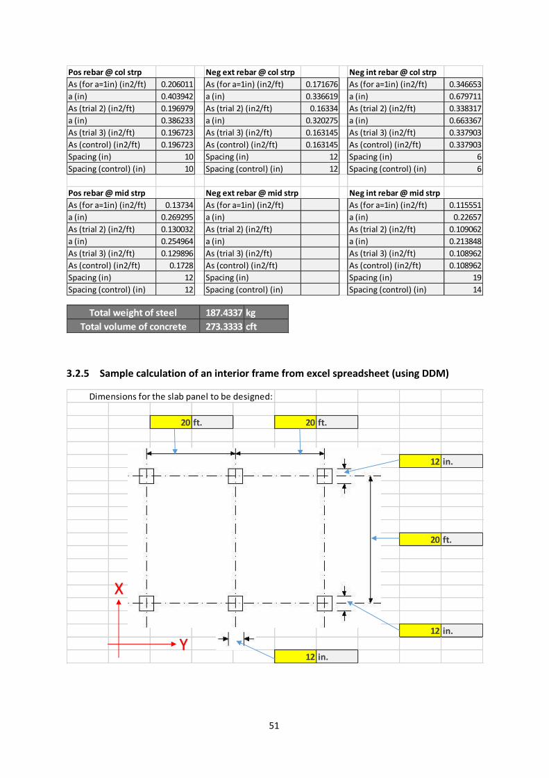
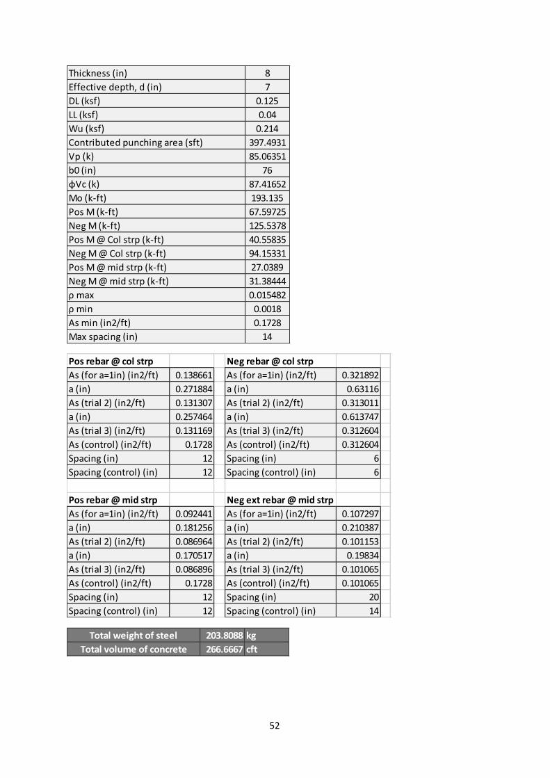
3.2.5 Sample calculation of an interior frame from excel spreadsheet (using DDM)
Pos rebar @ col strp Neg ext rebar @ col strp Neg int rebar @ col strp
As (for a=1in) (in2/ft) 0.206011 As (for a=1in) (in2/ft) 0.171676 As (for a=1in) (in2/ft) 0.346653
a (in) 0.403942 a (in) 0.336619 a (in) 0.679711
As (trial 2) (in2/ft) 0.196979 As (trial 2) (in2/ft) 0.16334 As (trial 2) (in2/ft) 0.338317
a (in) 0.386233 a (in) 0.320275 a (in) 0.663367
As (trial 3) (in2/ft) 0.196723 As (trial 3) (in2/ft) 0.163145 As (trial 3) (in2/ft) 0.337903
As (control) (in2/ft) 0.196723 As (control) (in2/ft) 0.163145 As (control) (in2/ft) 0.337903
Spacing (in) 10 Spacing (in) 12 Spacing (in) 6
Spacing (control) (in) 10 Spacing (control) (in) 12 Spacing (control) (in) 6
Pos rebar @ mid strp Neg ext rebar @ mid strp Neg int rebar @ mid strp
As (for a=1in) (in2/ft) 0.13734 As (for a=1in) (in2/ft) As (for a=1in) (in2/ft) 0.115551
a (in) 0.269295 a (in) a (in) 0.22657
As (trial 2) (in2/ft) 0.130032 As (trial 2) (in2/ft) As (trial 2) (in2/ft) 0.109062
a (in) 0.254964 a (in) a (in) 0.213848
As (trial 3) (in2/ft) 0.129896 As (trial 3) (in2/ft) As (trial 3) (in2/ft) 0.108962
As (control) (in2/ft) 0.1728 As (control) (in2/ft) As (control) (in2/ft) 0.108962
Spacing (in) 12 Spacing (in) Spacing (in) 19
Spacing (control) (in) 12 Spacing (control) (in) Spacing (control) (in) 14
187.4337 kg
273.3333 cft
Total weight of steel
Total volume of concrete
20 ft. 20 ft.
12 in.
20 ft.
12 in.
12 in.
Dimensions for the slab panel to be designed:
X
Y
52
Thickness (in) 8
Effective depth, d (in) 7
DL (ksf) 0.125
LL (ksf) 0.04
Wu (ksf) 0.214
Contributed punching area (sft) 397.4931
Vp (k) 85.06351
b0 (in) 76
φVc (k) 87.41652
Mo (k-ft) 193.135
Pos M (k-ft) 67.59725
Neg M (k-ft) 125.5378
Pos M @ Col strp (k-ft) 40.55835
Neg M @ Col strp (k-ft) 94.15331
Pos M @ mid strp (k-ft) 27.0389
Neg M @ mid strp (k-ft) 31.38444
ρ max 0.015482
ρ min 0.0018
As min (in2/ft) 0.1728
Max spacing (in) 14
Pos rebar @ col strp Neg rebar @ col strp
As (for a=1in) (in2/ft) 0.138661 As (for a=1in) (in2/ft) 0.321892
a (in) 0.271884 a (in) 0.63116
As (trial 2) (in2/ft) 0.131307 As (trial 2) (in2/ft) 0.313011
a (in) 0.257464 a (in) 0.613747
As (trial 3) (in2/ft) 0.131169 As (trial 3) (in2/ft) 0.312604
As (control) (in2/ft) 0.1728 As (control) (in2/ft) 0.312604
Spacing (in) 12 Spacing (in) 6
Spacing (control) (in) 12 Spacing (control) (in) 6
Pos rebar @ mid strp Neg ext rebar @ mid strp
As (for a=1in) (in2/ft) 0.092441 As (for a=1in) (in2/ft) 0.107297
a (in) 0.181256 a (in) 0.210387
As (trial 2) (in2/ft) 0.086964 As (trial 2) (in2/ft) 0.101153
a (in) 0.170517 a (in) 0.19834
As (trial 3) (in2/ft) 0.086896 As (trial 3) (in2/ft) 0.101065
As (control) (in2/ft) 0.1728 As (control) (in2/ft) 0.101065
Spacing (in) 12 Spacing (in) 20
Spacing (control) (in) 12 Spacing (control) (in) 14
203.8088 kg
266.6667 cft
Total weight of steel
Total volume of concrete
53
3.3 Beam-supported slab
Step 1: At first, we studied how to design a beam-supported slab by Direct Design Method,
from text-books and ACI codes.
Step 2: We designed one interior frame and one exterior frame, by hand calculation, to get
familiar with the design procedure.
Step 3: After understanding the design procedure properly, we started to formulate excel
spreadsheets, based on what we learnt on previous two steps. Two separate spreadsheets
were formulated to design both interior and exterior frames. Those were prepared in way
that it would take c/c span lengths of a frame, largest spans along both axes of the floor,
column cross-sections, slab-thickness, and different design data as inputs; and would give
outputs: slab thickness, bending-moments in both column and middle strips, rebar detailing
(showing rebar diameter, spacing and cut-off lengths), width of column and middle strips,
and estimated materials (weight of reinforcing steel and volume of concrete).
Step 4: As per table 3.1, inputs were put in the spreadsheets to design and estimate the floors.
The first task to work with the spreadsheets was the determination of the slab thickness,
which were based on three criteria:
Minimum thickness to control deflections, established by ACI code 9.5.3.3
Minimum effective depth for maximum reinforcement ratios, established by ACI
code 10.3.5
Minimum thickness to satisfy ACI code 9.5.3.3(c)
The worksheets were formulated in such a way that users not only can input the slab
thickness, but also see suggested thicknesses satisfying those three conditions (based on the
input thickness). So, at first, an assumed thickness had been input in the worksheets for the
frame having the largest clear span of the floor, and then observing the other suggestions,
input thickness was being changed simultaneously. At the last stage, a thickness had been
input that satisfied all the criteria, and not exceeding them. Then that thickness was put in
the worksheet for all the frames of a same floor.
Step 5: After designing all the frames and estimation of a floor, estimated material quantities
from outputs of those spreadsheets, were summed to estimate total material quantity for
the designed floor-system. By the same approach, all the floors were estimated shown in
table 3.1.
Step 6: Using all the estimated material quantities for different floors, were used to calculate
costs. For cost analysis, the considered types of costs were assumed same as flat-plate. Those
three types of costs were summed and expressed as per square-feet of floor area, which were
the total cost for a certain floor.
Step 7: Using the total material quantities and total costs, different column-charts had been
developed to interpret cost analysis. Those charts are shown in chapter 5.
54
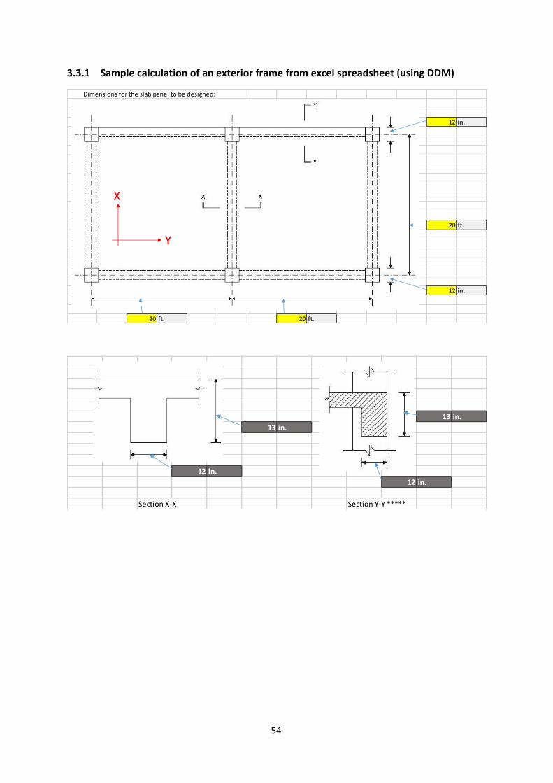
3.3.1 Sample calculation of an exterior frame from excel spreadsheet (using DDM)
12 in.
20 ft.
12 in.
20 ft. 20 ft.
Dimensions for the slab panel to be designed:
X
Y
13 in.
13 in.
12 in.
12 in.
Section X-X Section Y-Y *****
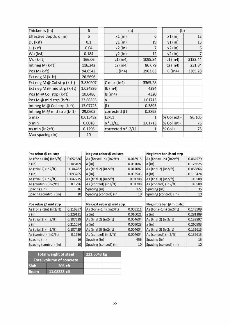
55
Thickness (in) 6
Effective depth, d (in) 5 x1 (in) 6 x1 (in) 12
DL (ksf) 0.1 y1 (in) 19 y1 (in) 13
LL (ksf) 0.04 x2 (in) 7 x2 (in) 6
Wu (ksf) 0.184 y2 (in) 12 y2 (in) 7
Mo (k-ft) 166.06 c1 (in4) 1095.84 c1 (in4) 3133.44
Int neg M (k-ft) 116.242 c2 (in4) 867.79 c2 (in4) 231.84
Pos M (k-ft) 94.6542 C (in4) 1963.63 C (in4) 3365.28
Ext neg M (k-ft) 26.5696
Ext neg M @ Col strp (k-ft) 3.830207 C max (in4) 3365.28
Ext neg M @ mid strp (k-ft) 1.034886 Ib (in4) 4394
Pos M @ Col strp (k-ft) 10.6486 Is (in4) 4320
Pos M @ mid strp (k-ft) 23.66355 α 1.01713
Int neg M @ Col strp (k-ft) 13.07723 β t 0.3895
Int neg M @ mid strp (k-ft) 29.0605 corrected β t 0.3895
ρ max 0.015482 L2/L1 1 % Col ext - 96.105
ρ min 0.0018 α*L2/L1 1.01713 % Col int - 75
As min (in2/ft) 0.1296 corrected α*L2/L1 1 % Col + 75
Max spacing (in) 10
(a) (b)
Pos rebar @ col strp Neg ext rebar @ col strp Neg int rebar @ col strp
As (for a=1in) (in2/ft) 0.052586 As (for a=1in) (in2/ft) 0.018915 As (for a=1in) (in2/ft) 0.064579
a (in) 0.103109 a (in) 0.037087 a (in) 0.126625
As (trial 2) (in2/ft) 0.04782 As (trial 2) (in2/ft) 0.017087 As (trial 2) (in2/ft) 0.058866
a (in) 0.093765 a (in) 0.033503 a (in) 0.115424
As (trial 3) (in2/ft) 0.047775 As (trial 3) (in2/ft) 0.01708 As (trial 3) (in2/ft) 0.0588
As (control) (in2/ft) 0.1296 As (control) (in2/ft) 0.01708 As (control) (in2/ft) 0.0588
Spacing (in) 16 Spacing (in) 122 Spacing (in) 35
Spacing (control) (in) 10 Spacing (control) (in) 10 Spacing (control) (in) 10
Pos rebar @ mid strp Neg ext rebar @ mid strp Neg int rebar @ mid strp
As (for a=1in) (in2/ft) 0.116857 As (for a=1in) (in2/ft) 0.005111 As (for a=1in) (in2/ft) 0.143509
a (in) 0.229131 a (in) 0.010021 a (in) 0.281389
As (trial 2) (in2/ft) 0.107638 As (trial 2) (in2/ft) 0.004604 As (trial 2) (in2/ft) 0.132897
a (in) 0.211054 a (in) 0.009028 a (in) 0.260583
As (trial 3) (in2/ft) 0.107439 As (trial 3) (in2/ft) 0.004604 As (trial 3) (in2/ft) 0.132613
As (control) (in2/ft) 0.1296 As (control) (in2/ft) 0.004604 As (control) (in2/ft) 0.132613
Spacing (in) 16 Spacing (in) 456 Spacing (in) 15
Spacing (control) (in) 10 Spacing (control) (in) 10 Spacing (control) (in) 10
221.6048 kg
Slab 205 cft
Beam 11.08333 cft
Total weight of steel
Total volume of concrete
56
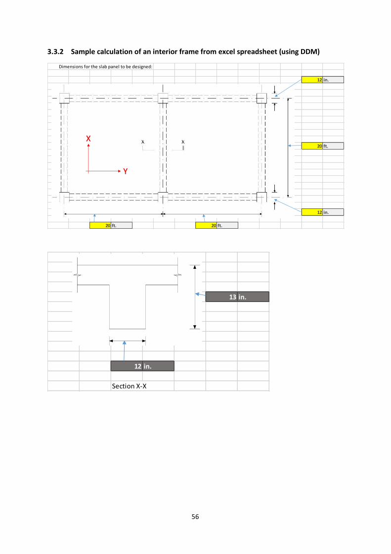
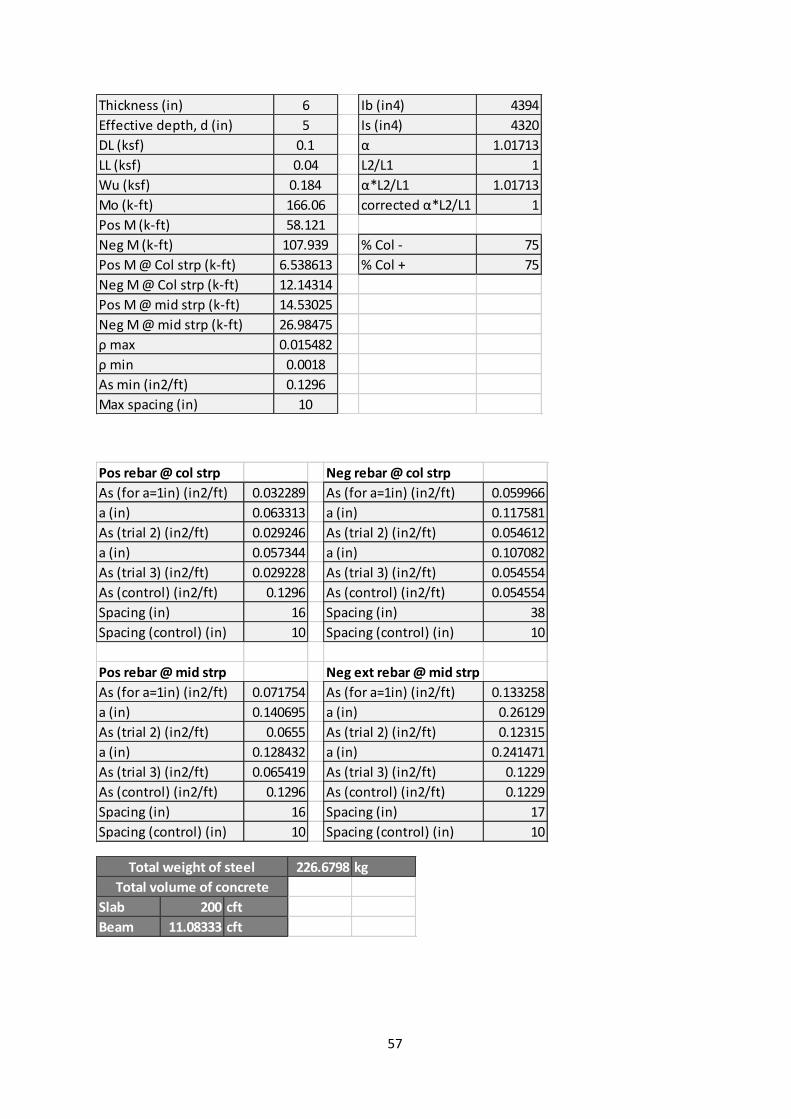
3.3.2 Sample calculation of an interior frame from excel spreadsheet (using DDM)
12 in.
20 ft.
12 in.
20 ft. 20 ft.
Dimensions for the slab panel to be designed:
X
Y
13 in.
12 in.
Section X-X
57
Thickness (in) 6 Ib (in4) 4394
Effective depth, d (in) 5 Is (in4) 4320
DL (ksf) 0.1 α 1.01713
LL (ksf) 0.04 L2/L1 1
Wu (ksf) 0.184 α*L2/L1 1.01713
Mo (k-ft) 166.06 corrected α*L2/L1 1
Pos M (k-ft) 58.121
Neg M (k-ft) 107.939 % Col - 75
Pos M @ Col strp (k-ft) 6.538613 % Col + 75
Neg M @ Col strp (k-ft) 12.14314
Pos M @ mid strp (k-ft) 14.53025
Neg M @ mid strp (k-ft) 26.98475
ρ max 0.015482
ρ min 0.0018
As min (in2/ft) 0.1296
Max spacing (in) 10
Pos rebar @ col strp Neg rebar @ col strp
As (for a=1in) (in2/ft) 0.032289 As (for a=1in) (in2/ft) 0.059966
a (in) 0.063313 a (in) 0.117581
As (trial 2) (in2/ft) 0.029246 As (trial 2) (in2/ft) 0.054612
a (in) 0.057344 a (in) 0.107082
As (trial 3) (in2/ft) 0.029228 As (trial 3) (in2/ft) 0.054554
As (control) (in2/ft) 0.1296 As (control) (in2/ft) 0.054554
Spacing (in) 16 Spacing (in) 38
Spacing (control) (in) 10 Spacing (control) (in) 10
Pos rebar @ mid strp Neg ext rebar @ mid strp
As (for a=1in) (in2/ft) 0.071754 As (for a=1in) (in2/ft) 0.133258
a (in) 0.140695 a (in) 0.26129
As (trial 2) (in2/ft) 0.0655 As (trial 2) (in2/ft) 0.12315
a (in) 0.128432 a (in) 0.241471
As (trial 3) (in2/ft) 0.065419 As (trial 3) (in2/ft) 0.1229
As (control) (in2/ft) 0.1296 As (control) (in2/ft) 0.1229
Spacing (in) 16 Spacing (in) 17
Spacing (control) (in) 10 Spacing (control) (in) 10
226.6798 kg
Slab 200 cft
Beam 11.08333 cft
Total volume of concrete
Total weight of steel
58
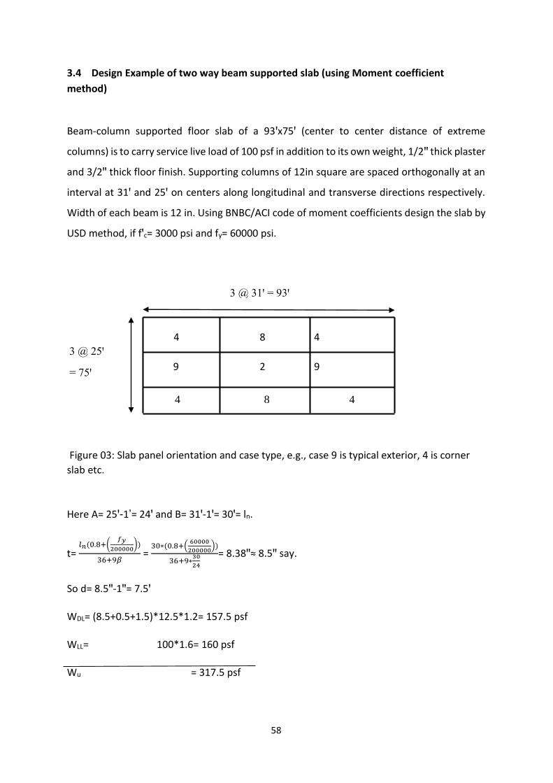
3.4 Design Example of two way beam supported slab (using Moment coefficient
method)
Beam-column supported floor slab of a 93ꞌx75ꞌ (center to center distance of extreme
columns) is to carry service live load of 100 psf in addition to its own weight, 1/2ꞌꞌ thick plaster
and 3/2ꞌꞌ thick floor finish. Supporting columns of 12in square are spaced orthogonally at an
interval at 31ꞌ and 25ꞌ on centers along longitudinal and transverse directions respectively.
Width of each beam is 12 in. Using BNBC/ACI code of moment coefficients design the slab by
USD method, if fꞌc= 3000 psi and fy= 60000 psi.
4 8 4
9 2 9
Figure 03: Slab panel orientation and case type, e.g., case 9 is typical exterior, 4 is corner
slab etc.
Here A= 25ꞌ-1’= 24ꞌ and B= 31ꞌ-1ꞌ= 30ꞌ= ln.
t= 𝑙𝑛 (0.8+(
𝑓𝑦
200000))
36+9𝛽 =
30∗(0.8+(60000
200000))
36+9∗30
24
= 8.38ꞌꞌ≈ 8.5ꞌꞌ say.
So d= 8.5ꞌꞌ-1ꞌꞌ= 7.5ꞌ
WDL= (8.5+0.5+1.5)*12.5*1.2= 157.5 psf
WLL= 100*1.6= 160 psf
Wu = 317.5 psf
3 @ 31ꞌ = 93ꞌ
3 @ 25ꞌ
= 75ꞌ
4 4 8
59
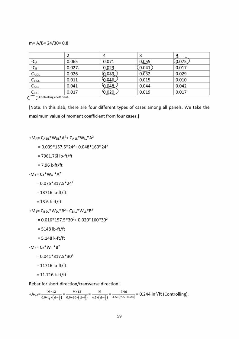
m= A/B= 24/30= 0.8
2 4 8 9
-CA 0.065 0.071 0.055 0.075
-CB 0.027. 0.029 0.041 0.017
CA DL 0.026 0.039 0.032 0.029
CB DL 0.011 0.016 0.015 0.010
CA LL 0.041 0.048 0.044 0.042
CB LL 0.017 0.020 0.019 0.017 Controlling coefficient.
[Note: In this slab, there are four different types of cases among all panels. We take the
maximum value of moment coefficient from four cases.]
+MA= CA DL*WDL*A2+ CA LL*WLL*A2
= 0.039*157.5*242+ 0.048*160*242
= 7961.76l lb-ft/ft
= 7.96 k-ft/ft
-MA= CA*Wu *A2
= 0.075*317.5*242
= 13716 lb-ft/ft
= 13.6 k-ft/ft
+MB= CB DL*WDL*B2+ CB LL*WLL*B2
= 0.016*157.5*302+ 0.020*160*302
= 5148 lb-ft/ft
= 5.148 k-ft/ft
-MB= CB*Wu *B2
= 0.041*317.5*302
= 11716 lb-ft/ft
= 11.716 k-ft/ft
Rebar for short direction/transverse direction:
+AS A= M∗12
0.9∗fy∗(d−a
2)
= M∗12
0.9∗60∗(d−a
2)
= M
4.5∗(d−a
2) =
7.96
4.5∗(7.5−0.24) = 0.244 in2/ft (Controlling).
60
and a =Asfy
0.85fc′ b
=As∗60
0.85∗3∗12 = 1.96*AS = 1.96*0.244 = 0.478 in.
Amin= 0.0018xbxt = 0.0018x12x8.5 = 0.1836 in2/ft
Using φ10mm bar
S = Area of bar used∗ width of strip
Requried As =
0.121∗12
0.244 = 5.95ꞌꞌ ≈ 5.5ꞌꞌc/c at bottom along short direction
crank 50% bar to negative zone.
-AS A= M
4.5∗(d−a
2) =
13.61
4.5∗(7.5−0.42) = 0.427 in2/ft (Controlling).
a = 1.96 ∗ As = 0.838 in
Amin= 0.1836 in2/ft.
Already provided As1= 0.121∗12
11= 0.132 in2/ft
Extra top required, As2= (0.427-0.132) = 0.295 in2/ft.
Using Φ10mm bar S= 4.92 ≈ 4.5ꞌꞌ c/c extra top.
Rebar along long direction:
+AS B= 5.148
4.5∗(7.5−0.15) = 0.155 in2/ft
Amin= 0.1836 in2/ft (Controlling).
Using Φ10 mm bar @ 7.90”≈7.5” c/c at bottom along long direction crank 50% bar to negative zone.
-AS B= 11.716
4.5∗(7.5−0.36) = 0.365 in2/ft
Already provided As1= 0.121∗12
15 = 0.0968in2/ft
Extra top required, As2= (0.365-00.0968) in2/ft = 0.2682 in2/ft
Using Φ 10mm bar @ 5.41” ≈ 5ꞌꞌ c/c extra top
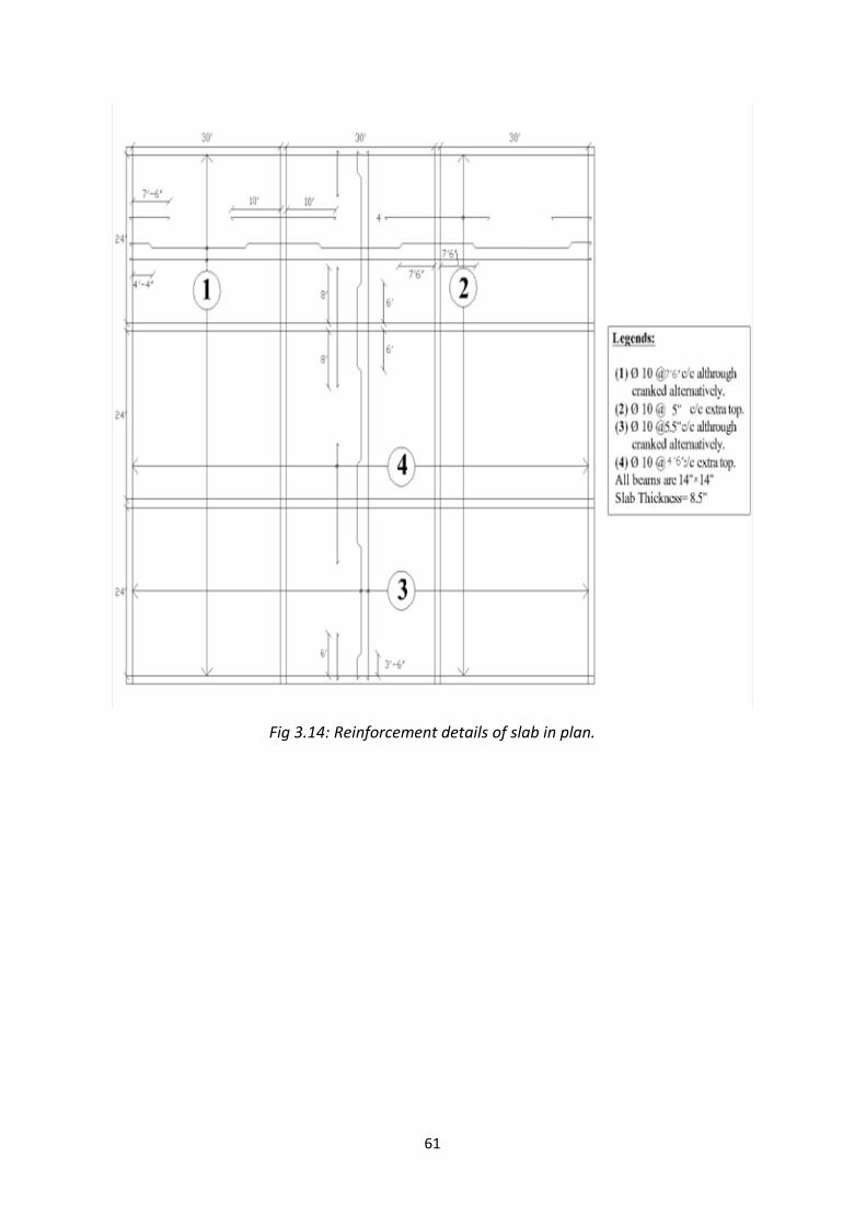
61
Fig 3.14: Reinforcement details of slab in plan.

62
Chapter 4
RESULTS & DISCUSSION
63
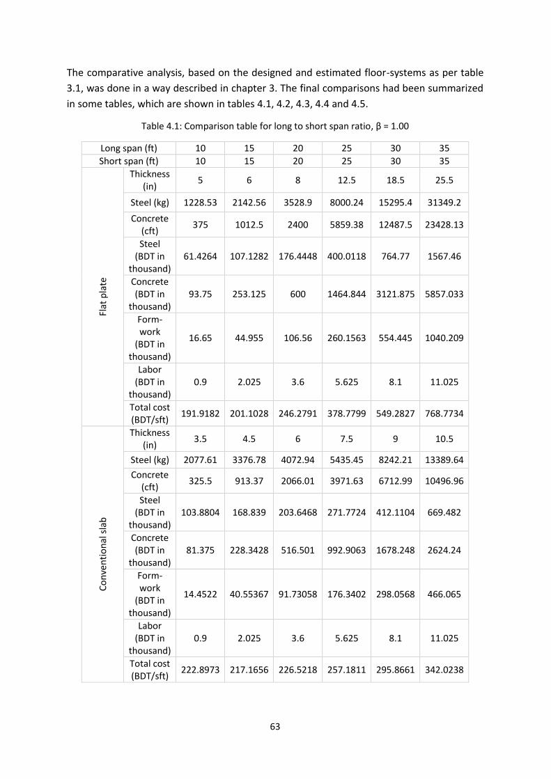
The comparative analysis, based on the designed and estimated floor-systems as per table
3.1, was done in a way described in chapter 3. The final comparisons had been summarized
in some tables, which are shown in tables 4.1, 4.2, 4.3, 4.4 and 4.5.
Table 4.1: Comparison table for long to short span ratio, β = 1.00
Long span (ft) 10 15 20 25 30 35
Short span (ft) 10 15 20 25 30 35
Flat
pla
te
Thickness (in)
5 6 8 12.5 18.5 25.5
Steel (kg) 1228.53 2142.56 3528.9 8000.24 15295.4 31349.2
Concrete (cft)
375 1012.5 2400 5859.38 12487.5 23428.13
Steel (BDT in
thousand) 61.4264 107.1282 176.4448 400.0118 764.77 1567.46
Concrete (BDT in
thousand) 93.75 253.125 600 1464.844 3121.875 5857.033
Form-work
(BDT in thousand)
16.65 44.955 106.56 260.1563 554.445 1040.209
Labor (BDT in
thousand) 0.9 2.025 3.6 5.625 8.1 11.025
Total cost (BDT/sft)
191.9182 201.1028 246.2791 378.7799 549.2827 768.7734
Co
nve
nti
on
al s
lab
Thickness (in)
3.5 4.5 6 7.5 9 10.5
Steel (kg) 2077.61 3376.78 4072.94 5435.45 8242.21 13389.64
Concrete (cft)
325.5 913.37 2066.01 3971.63 6712.99 10496.96
Steel (BDT in
thousand) 103.8804 168.839 203.6468 271.7724 412.1104 669.482
Concrete (BDT in
thousand) 81.375 228.3428 516.501 992.9063 1678.248 2624.24
Form-work
(BDT in thousand)
14.4522 40.55367 91.73058 176.3402 298.0568 466.065
Labor (BDT in
thousand) 0.9 2.025 3.6 5.625 8.1 11.025
Total cost (BDT/sft)
222.8973 217.1656 226.5218 257.1811 295.8661 342.0238
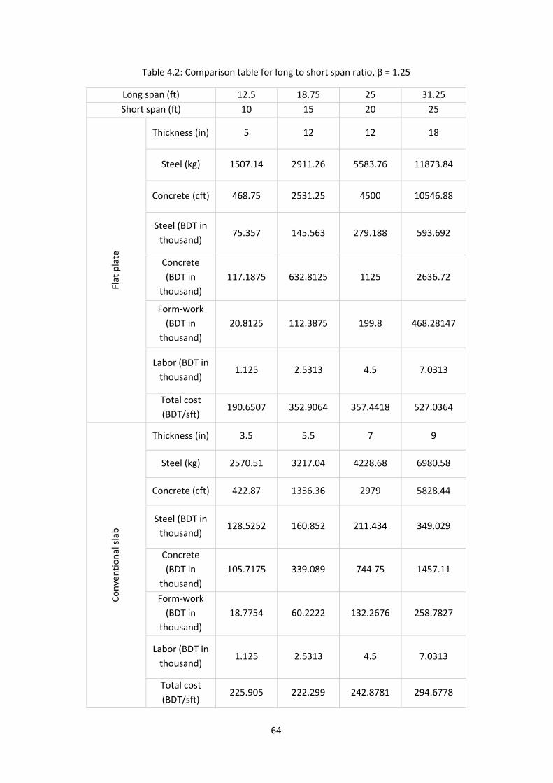
64
Table 4.2: Comparison table for long to short span ratio, β = 1.25
Long span (ft) 12.5 18.75 25 31.25
Short span (ft) 10 15 20 25 Fl
at p
late
Thickness (in) 5 12 12 18
Steel (kg) 1507.14 2911.26 5583.76 11873.84
Concrete (cft) 468.75 2531.25 4500 10546.88
Steel (BDT in
thousand) 75.357 145.563 279.188 593.692
Concrete
(BDT in
thousand)
117.1875 632.8125 1125 2636.72
Form-work
(BDT in
thousand)
20.8125 112.3875 199.8 468.28147
Labor (BDT in
thousand) 1.125 2.5313 4.5 7.0313
Total cost
(BDT/sft) 190.6507 352.9064 357.4418 527.0364
Co
nve
nti
on
al s
lab
Thickness (in) 3.5 5.5 7 9
Steel (kg) 2570.51 3217.04 4228.68 6980.58
Concrete (cft) 422.87 1356.36 2979 5828.44
Steel (BDT in
thousand) 128.5252 160.852 211.434 349.029
Concrete
(BDT in
thousand)
105.7175 339.089 744.75 1457.11
Form-work
(BDT in
thousand)
18.7754 60.2222 132.2676 258.7827
Labor (BDT in
thousand) 1.125 2.5313 4.5 7.0313
Total cost
(BDT/sft) 225.905 222.299 242.8781 294.6778
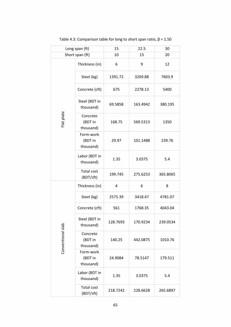
65
Table 4.3: Comparison table for long to short span ratio, β = 1.50
Long span (ft) 15 22.5 30
Short span (ft) 10 15 20
Flat
pla
te
Thickness (in) 6 9 12
Steel (kg) 1391.72 3269.88 7603.9
Concrete (cft) 675 2278.13 5400
Steel (BDT in
thousand) 69.5858 163.4942 380.195
Concrete
(BDT in
thousand)
168.75 569.5313 1350
Form-work
(BDT in
thousand)
29.97 101.1488 239.76
Labor (BDT in
thousand) 1.35 3.0375 5.4
Total cost
(BDT/sft) 199.745 275.6253 365.8065
Co
nve
nti
on
al s
lab
Thickness (in) 4 6 8
Steel (kg) 2575.39 3418.47 4781.07
Concrete (cft) 561 1768.35 4043.04
Steel (BDT in
thousand) 128.7693 170.9234 239.0534
Concrete
(BDT in
thousand)
140.25 442.0875 1010.76
Form-work
(BDT in
thousand)
24.9084 78.5147 179.511
Labor (BDT in
thousand) 1.35 3.0375 5.4
Total cost
(BDT/sft) 218.7242 228.6628 265.6897
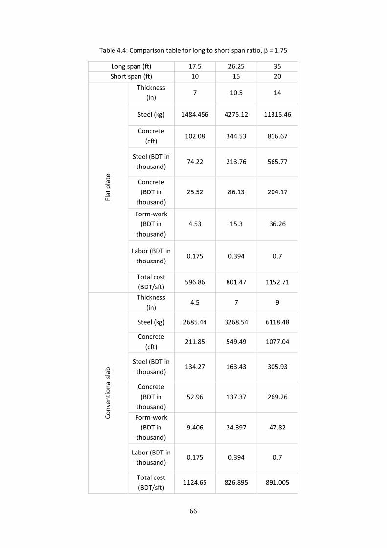
66
Table 4.4: Comparison table for long to short span ratio, β = 1.75
Long span (ft) 17.5 26.25 35
Short span (ft) 10 15 20
Flat
pla
te
Thickness
(in) 7 10.5 14
Steel (kg) 1484.456 4275.12 11315.46
Concrete
(cft) 102.08 344.53 816.67
Steel (BDT in
thousand) 74.22 213.76 565.77
Concrete
(BDT in
thousand)
25.52 86.13 204.17
Form-work
(BDT in
thousand)
4.53 15.3 36.26
Labor (BDT in
thousand) 0.175 0.394 0.7
Total cost
(BDT/sft) 596.86 801.47 1152.71
Co
nve
nti
on
al s
lab
Thickness
(in) 4.5 7 9
Steel (kg) 2685.44 3268.54 6118.48
Concrete
(cft) 211.85 549.49 1077.04
Steel (BDT in
thousand) 134.27 163.43 305.93
Concrete
(BDT in
thousand)
52.96 137.37 269.26
Form-work
(BDT in
thousand)
9.406 24.397 47.82
Labor (BDT in
thousand) 0.175 0.394 0.7
Total cost
(BDT/sft) 1124.65 826.895 891.005
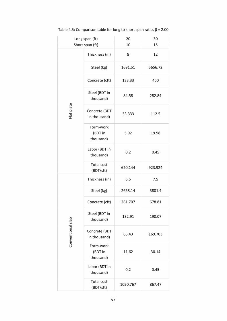
67
Table 4.5: Comparison table for long to short span ratio, β = 2.00
Long span (ft) 20 30
Short span (ft) 10 15
Flat
pla
te
Thickness (in) 8 12
Steel (kg) 1691.51 5656.72
Concrete (cft) 133.33 450
Steel (BDT in
thousand) 84.58 282.84
Concrete (BDT
in thousand) 33.333 112.5
Form-work
(BDT in
thousand)
5.92 19.98
Labor (BDT in
thousand) 0.2 0.45
Total cost
(BDT/sft) 620.144 923.924
Co
nve
nti
on
al s
lab
Thickness (in) 5.5 7.5
Steel (kg) 2658.14 3801.4
Concrete (cft) 261.707 678.81
Steel (BDT in
thousand) 132.91 190.07
Concrete (BDT
in thousand) 65.43 169.703
Form-work
(BDT in
thousand)
11.62 30.14
Labor (BDT in
thousand) 0.2 0.45
Total cost
(BDT/sft) 1050.767 867.47
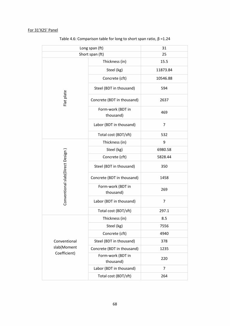
68
For 31’X25’ Panel
Table 4.6: Comparison table for long to short span ratio, β =1.24
Long span (ft) 31
Short span (ft) 25
Flat
pla
te
Thickness (in) 15.5
Steel (kg) 11873.84
Concrete (cft) 10546.88
Steel (BDT in thousand) 594
Concrete (BDT in thousand) 2637
Form-work (BDT in
thousand) 469
Labor (BDT in thousand) 7
Total cost (BDT/sft) 532
Co
nve
nti
on
al s
lab
(Dir
ect
Des
ign
)
Thickness (in) 9
Steel (kg) 6980.58
Concrete (cft) 5828.44
Steel (BDT in thousand) 350
Concrete (BDT in thousand) 1458
Form-work (BDT in
thousand) 269
Labor (BDT in thousand) 7
Total cost (BDT/sft) 297.1
Conventional
slab(Moment
Coefficient)
Thickness (in) 8.5
Steel (kg) 7556
Concrete (cft) 4940
Steel (BDT in thousand) 378
Concrete (BDT in thousand) 1235
Form-work (BDT in
thousand) 220
Labor (BDT in thousand) 7
Total cost (BDT/sft) 264
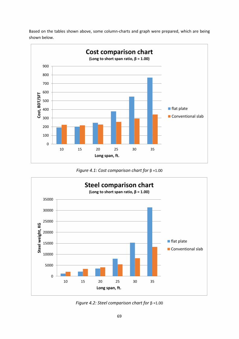
69
Based on the tables shown above, some column-charts and graph were prepared, which are being
shown below.
Figure 4.1: Cost comparison chart for β =1.00
Figure 4.2: Steel comparison chart for β =1.00
0
100
200
300
400
500
600
700
800
900
10 15 20 25 30 35
Co
st, B
DT/
SFT
Long span, ft.
Cost comparison chart(Long to short span ratio, β = 1.00)
flat plate
Conventional slab
0
5000
10000
15000
20000
25000
30000
35000
10 15 20 25 30 35
Ste
el w
eigh
t, K
G
Long span, ft.
Steel comparison chart(Long to short span ratio, β = 1.00)
flat plate
Conventional slab
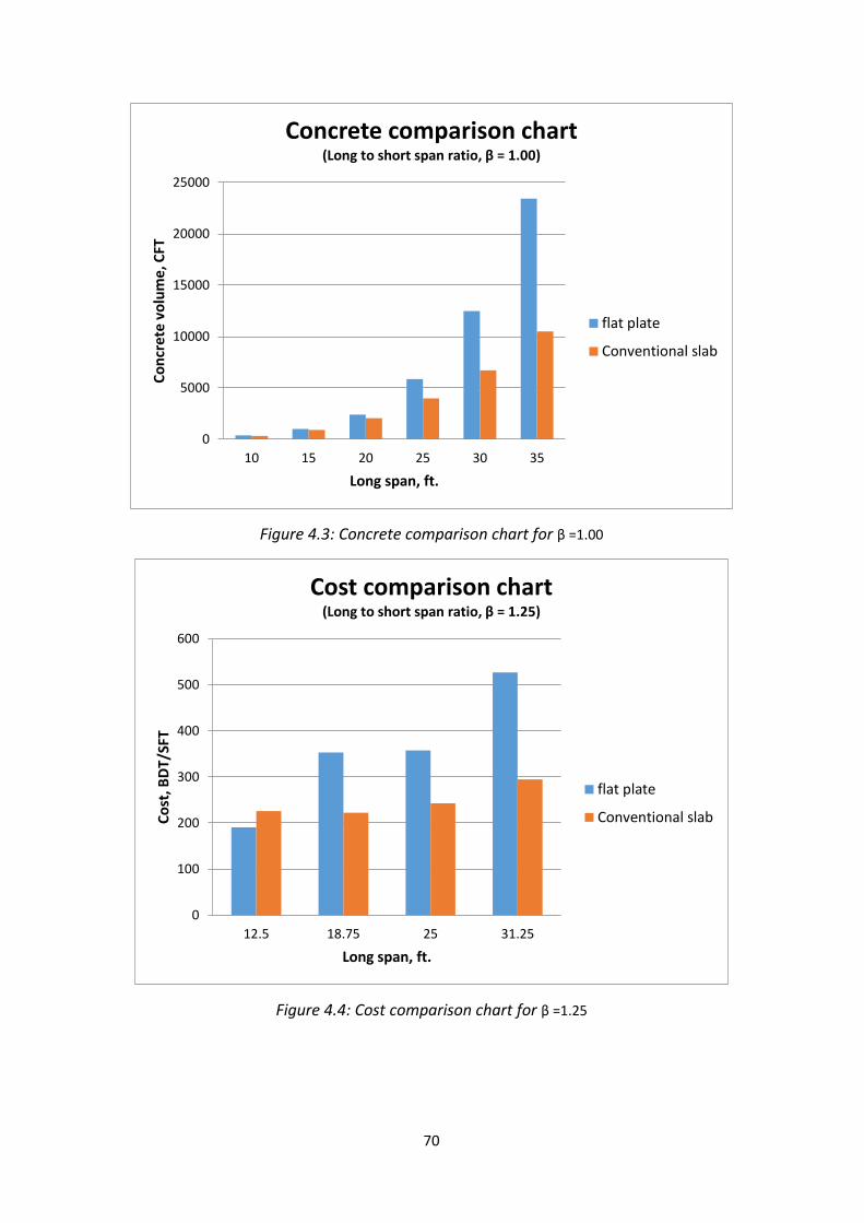
70
Figure 4.3: Concrete comparison chart for β =1.00
Figure 4.4: Cost comparison chart for β =1.25
0
5000
10000
15000
20000
25000
10 15 20 25 30 35
Co
ncr
ete
vo
lum
e, C
FT
Long span, ft.
Concrete comparison chart(Long to short span ratio, β = 1.00)
flat plate
Conventional slab
0
100
200
300
400
500
600
12.5 18.75 25 31.25
Co
st, B
DT/
SFT
Long span, ft.
Cost comparison chart(Long to short span ratio, β = 1.25)
flat plate
Conventional slab
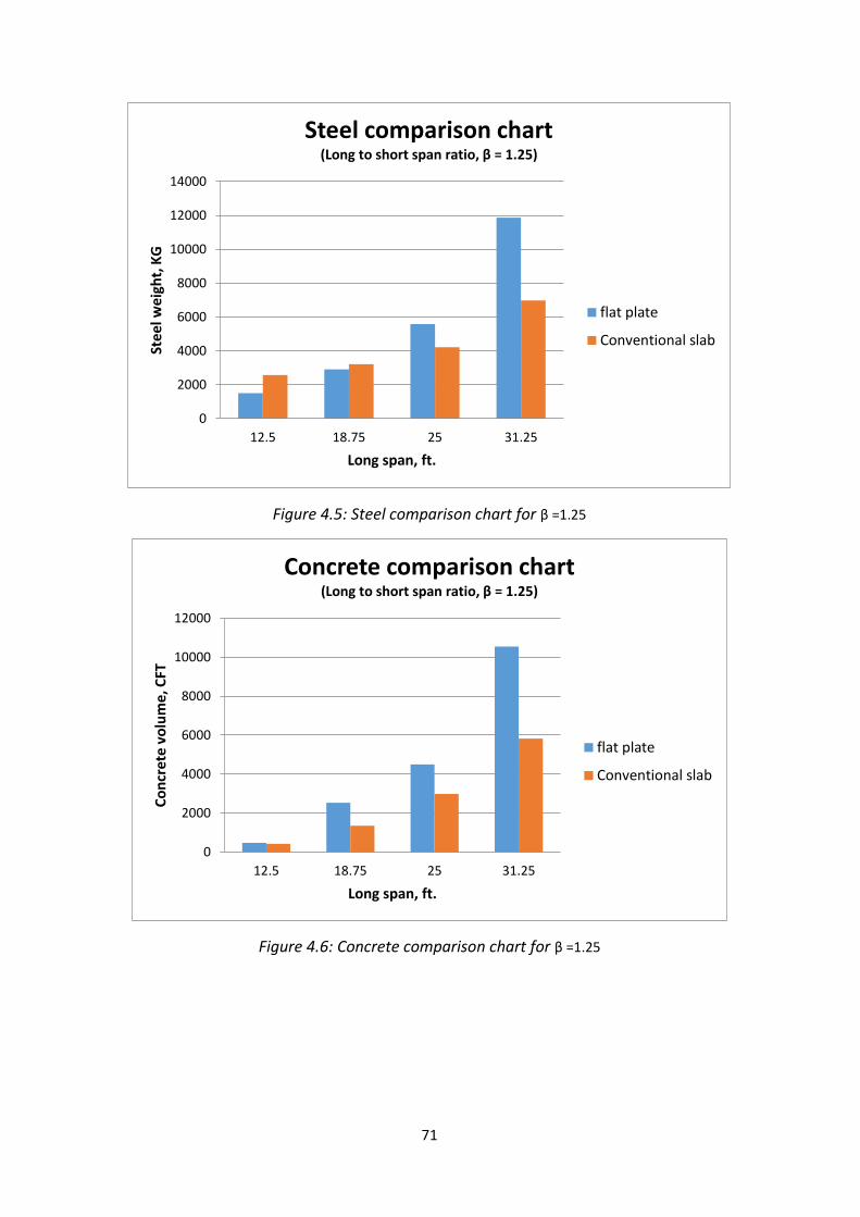
71
Figure 4.5: Steel comparison chart for β =1.25
Figure 4.6: Concrete comparison chart for β =1.25
0
2000
4000
6000
8000
10000
12000
14000
12.5 18.75 25 31.25
Ste
el w
eigh
t, K
G
Long span, ft.
Steel comparison chart(Long to short span ratio, β = 1.25)
flat plate
Conventional slab
0
2000
4000
6000
8000
10000
12000
12.5 18.75 25 31.25
Co
ncr
ete
vo
lum
e, C
FT
Long span, ft.
Concrete comparison chart(Long to short span ratio, β = 1.25)
flat plate
Conventional slab
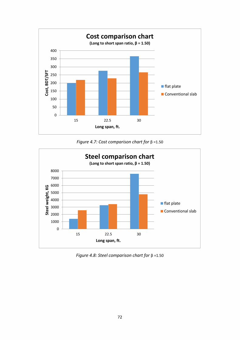
72
Figure 4.7: Cost comparison chart for β =1.50
Figure 4.8: Steel comparison chart for β =1.50
0
50
100
150
200
250
300
350
400
15 22.5 30
Co
st, B
DT/
SFT
Long span, ft.
Cost comparison chart(Long to short span ratio, β = 1.50)
flat plate
Conventional slab
0
1000
2000
3000
4000
5000
6000
7000
8000
15 22.5 30
Ste
el w
eig
ht,
KG
Long span, ft.
Steel comparison chart(Long to short span ratio, β = 1.50)
flat plate
Conventional slab
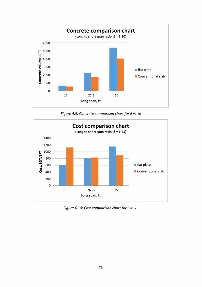
73
Figure 4.9: Concrete comparison chart for β =1.50
Figure 4.10: Cost comparison chart for β =1.75
0
1000
2000
3000
4000
5000
6000
15 22.5 30
Co
ncr
ete
vo
lum
e, C
FT
Long span, ft.
Concrete comparison chart(Long to short span ratio, β = 1.50)
flat plate
Conventional slab
0
200
400
600
800
1000
1200
1400
17.5 26.25 35
Co
st, B
DT/
SFT
Long span, ft.
Cost comparison chart(Long to short span ratio, β = 1.75)
flat plate
Conventional slab
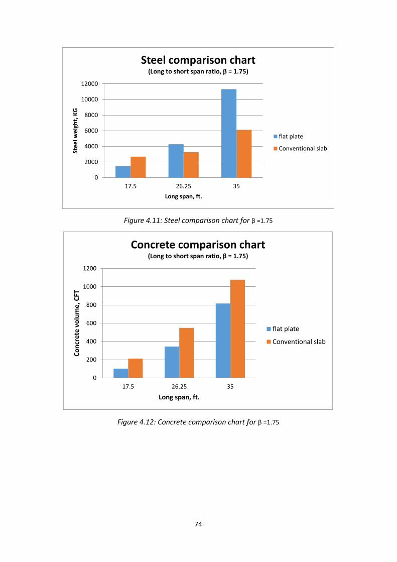
74
Figure 4.11: Steel comparison chart for β =1.75
Figure 4.12: Concrete comparison chart for β =1.75
0
2000
4000
6000
8000
10000
12000
17.5 26.25 35
Ste
el w
eig
ht,
KG
Long span, ft.
Steel comparison chart(Long to short span ratio, β = 1.75)
flat plate
Conventional slab
0
200
400
600
800
1000
1200
17.5 26.25 35
Co
ncr
ete
vo
lum
e, C
FT
Long span, ft.
Concrete comparison chart(Long to short span ratio, β = 1.75)
flat plate
Conventional slab
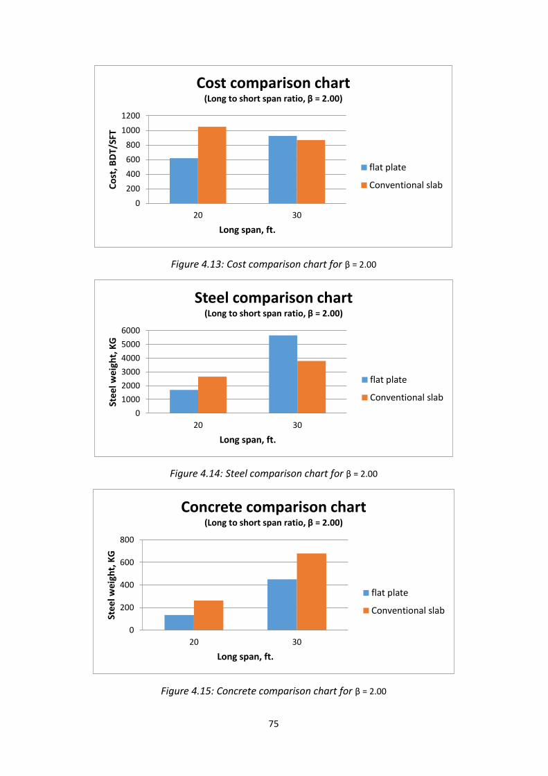
75
Figure 4.13: Cost comparison chart for β = 2.00
Figure 4.14: Steel comparison chart for β = 2.00
Figure 4.15: Concrete comparison chart for β = 2.00
0
200
400
600
800
1000
1200
20 30
Co
st, B
DT/
SFT
Long span, ft.
Cost comparison chart(Long to short span ratio, β = 2.00)
flat plate
Conventional slab
0
1000
2000
3000
4000
5000
6000
20 30
Ste
el w
eig
ht,
KG
Long span, ft.
Steel comparison chart(Long to short span ratio, β = 2.00)
flat plate
Conventional slab
0
200
400
600
800
20 30
Ste
el w
eigh
t, K
G
Long span, ft.
Concrete comparison chart(Long to short span ratio, β = 2.00)
flat plate
Conventional slab
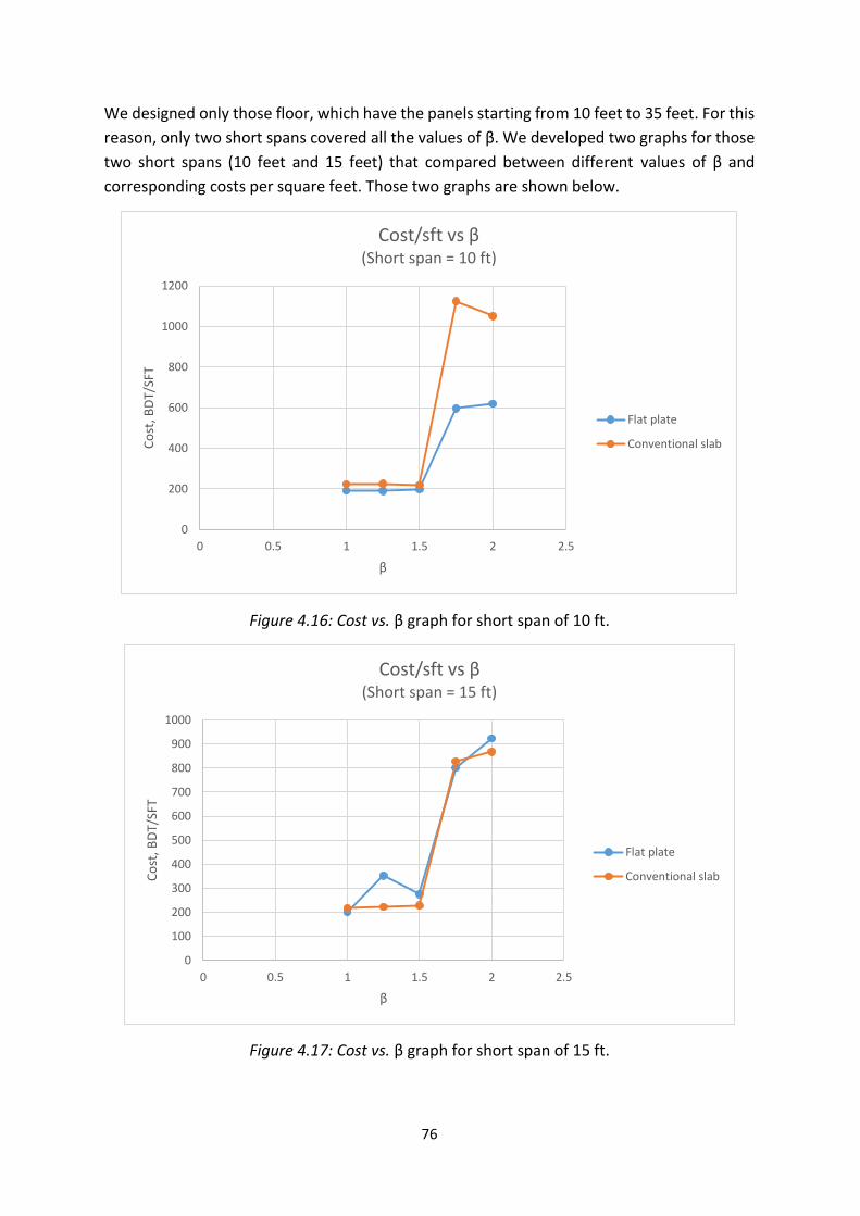
76
We designed only those floor, which have the panels starting from 10 feet to 35 feet. For this
reason, only two short spans covered all the values of β. We developed two graphs for those
two short spans (10 feet and 15 feet) that compared between different values of β and
corresponding costs per square feet. Those two graphs are shown below.
Figure 4.16: Cost vs. β graph for short span of 10 ft.
Figure 4.17: Cost vs. β graph for short span of 15 ft.
0
200
400
600
800
1000
1200
0 0.5 1 1.5 2 2.5
Co
st, B
DT/
SFT
β
Cost/sft vs β(Short span = 10 ft)
Flat plate
Conventional slab
0
100
200
300
400
500
600
700
800
900
1000
0 0.5 1 1.5 2 2.5
Co
st, B
DT/
SFT
β
Cost/sft vs β(Short span = 15 ft)
Flat plate
Conventional slab
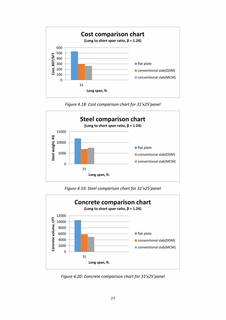
77
Figure 4.18: Cost comparison chart for 31’x25’panel
Figure 4.19: Steel comparison chart for 31’x25’panel
Figure 4.20: Concrete comparison chart for 31’x25’panel
0
100
200
300
400
500
600
31
Co
st, B
DT/
SFT
Long span, ft.
Cost comparison chart(Long to short span ratio, β = 1.24)
flat plate
conventional slab(DDM)
conventional slab(MCM)
0
5000
10000
15000
31
Ste
el w
eig
ht,
KG
Long span, ft.
Steel comparison chart(Long to short span ratio, β = 1.24)
flat plate
conventional slab(DDM)
conventional slab(MCM)
0
2000
4000
6000
8000
10000
12000
31
Co
ncr
ete
vo
lum
e, C
FT
Long span, ft.
Concrete comparison chart(Long to short span ratio, β = 1.24)
flat plate
conventional slab(DDM)
conventional slab(MCM)

78
Chapter 5
CONCLUSION
79
5.1 Limitations
This research work was done based with specifications from ACI 318-11 and BNBC 2006. Only
gravity loads, i.e. dead load and live load, had been considered for design. If others loads,
aside those two loads, have to be considered, the slabs should be analyzed and designed
separately. The floors that had been considered in here, have equal panel sizes. If panel sizes
differ, the recommendations of this research cannot be followed but for similar type of floors,
i.e. equal spanning floor in same direction. The flat-plates, been designed, were considered
having no edge beams. Some of the design data were considered constant, e.g. material
strength, bar size, loads, etc. to compare the results evenly.
To mitigate some difficulties in calculations, some approximations were considered in this
thesis. So a few limitations have been induced in the results. Such as –
Conservative calculations were done to estimate material quantities.
For conventional beam-supported slabs, straight bars were used instead of cranked
bars which is more economical solution than straight bars.
The depth of the beam was assumed as the minimum depth specified by ACI code:
table 9.5(a).
Beam reinforcement was not designed.
For beam-supported slabs, αfm has been considered greater than 2.0.
For beam-supported slabs, punching shear was not checked, which is not needed
because of having shear reinforcement in beams.
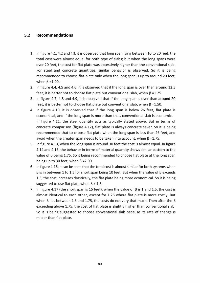
80
5.2 Recommendations
1. In figure 4.1, 4.2 and 4.3, it is observed that long span lying between 10 to 20 feet, the
total cost were almost equal for both type of slabs; but when the long spans were
over 20 feet, the cost for flat plate was excessively higher than the conventional slab.
For steel and concrete quantities, similar behavior is observed. So it is being
recommended to choose flat-plate only when the long span is up to around 20 feet,
when β =1.00.
2. In figure 4.4, 4.5 and 4.6, it is observed that if the long span is over than around 12.5
feet, it is better not to choose flat plate but conventional slab, when β =1.25.
3. In figure 4.7, 4.8 and 4.9, it is observed that if the long span is over than around 20
feet, it is better not to choose flat plate but conventional slab, when β =1.50.
4. In figure 4.10, it is observed that if the long span is below 26 feet, flat plate is
economical, and if the long span is more than that, conventional slab is economical.
In figure 4.11, the steel quantity acts as typically stated above. But in terms of
concrete comparison (figure 4.12), flat plate is always concrete saver. So it is being
recommended that to choose flat plate when the long span is less than 26 feet, and
avoid when the greater span needs to be taken into account, when β =1.75.
5. In figure 4.13, when the long span is around 30 feet the cost is almost equal. In figure
4.14 and 4.15, the behavior in terms of material quantity shows similar pattern to the
value of β being 1.75. So it being recommended to choose flat plate at the long span
being up to 30 feet, when β =2.00.
6. In figure 4.16, it can be seen that the total cost is almost similar for both systems when
β is in between 1 to 1.5 for short span being 10 feet. But when the value of β exceeds
1.5, the cost increases drastically, the flat plate being more economical. So it is being
suggested to use flat plate when β > 1.5.
7. In figure 4.17 (the short span is 15 feet), when the value of β is 1 and 1.5, the cost is
almost identical to each other, except for 1.25 where flat plate is more costly. But
when β lies between 1.5 and 1.75, the costs do not vary that much. Then after the β
exceeding above 1.75, the cost of flat plate is slightly higher than conventional slab.
So it is being suggested to choose conventional slab because its rate of change is
milder than flat plate.
81
5.3 Conclusion
In a nutshell, it can be said that flat plate is cost effective for the long span being up to 20 feet
approximately, when the slab-panels are exactly or almost square shaped. Otherwise,
conventional beam-supported slabs are more economical than flat plate, especially for floors
with larger spanning panels.
In spite of all of those limitations mentioned in article 5.1, this research work can give a rough
idea about the cost comparison between flat-plate and conventional beam-supported slab;
and people, both practicing engineers, architects, and non-technical persons, can decide
which floor-system is more economical than the other one for what spans and span-ratio;
which is the main purpose of this thesis.
This thesis paper will also pave the way for further investigations for more than 35 feet
spanned panels, considering other types of floor-systems, e.g. flat-slabs with or without drop-
panels/column-capital, one-way ribbed slab, waffle slab, hollow-core slab, advanced
composite type slabs, etc.
In this research work, some excel spreadsheets were prepared as mentioned earlier. Those
spreadsheets would help the designers and those who are interested in designing flat-plate
and beam-supported slabs, to conduct preliminary design in the shortest possible time, with
minimum amount of effort.
82
REFERENCES
I. Simplified Design of Reinforced Concrete Buildings, Mahmoud E. Kamara and
Lawrence C. Novak, Fourth Edition.
II. Bangladesh National Building Code, (BNBC 2006)
III. Building Code Requirements for Reinforced Concrete, American Concrete
Institute (ACI 318-63).
IV. International Building Code (ICC or IBC 2012).
V. Uniform Building Code, (UBC 1997 Volume 02).
VI. Design of Concrete Structures, Arthur H. Nilson, David Darwin and Charles W.
Dolan, Fourteenth Edition.
VII. Design of Concrete Structures, George Winter, C. E. O’Rourke, L. C. Urquhart
and Arthur H. Nilson, Seventh Edition.
VIII. Design of Reinforced Concrete Floor Systems, David A. Fanella and Iyad M.
Alsamsam.
IX. An Engineers Guide To: Economical Concrete Floor Systems
X. Design of Reinforced Concrete, Jack C. McCormack, Russel H. Brown, Ninth
Edition
XI. Building code requirements for structural concrete ACI 318-11 and Comentary-
American concrete institute, Farmington’s Hills, Michigan 2011.
XII. Building Movements and Joints, EB 086, Portland Cement Association, Skokie,
Illinois, 1982, 64 pp.
XIII. Concrete Floor system-Guide to Estimating and Economizing, SP041, Portland
Cement Association, Skokie, Illinois, 2000, 41 pp.
XIV. Long Span Concrete Floor Systems, SP339, Portland Cement Association, Skokie,
Illinois, 2000, 97 pp.
XV. American Society of Civil Engineers, Minimum Design Loads for Building and
other Structures. ASCE/SEI 7-05.American Society of Civil Engineers, New York,
NY, 2006.