COMPARATIVE STUDY OF HOLT-WINTERS TRIPLE EXPONENTIAL … · TRIPLE EXPONENTIAL SMOOTHING AND SEASONAL ARIMA: FORECASTING SHORT TERM SEASONAL CAR SALES IN SOUTH AFRICA Katleho Daniel

Risk governance & control: financial markets & institutions / Volume 6, Issue 1, Winter 2016

71

COMPARATIVE STUDY OF HOLT-WINTERS

TRIPLE EXPONENTIAL SMOOTHING AND

SEASONAL ARIMA: FORECASTING SHORT TERM

SEASONAL CAR SALES IN SOUTH AFRICA

Katleho Daniel Makatjane*, Ntebogang Dinah Moroke*

* North West University, P/ Bag X2046, Mmabatho, 2735, South Africa

Abstract

In this paper, both Seasonal ARIMA and Holt-Winters models are developed to predict the monthly car sales in South Africa using data for the period of January 1994 to December 2013. The purpose of this study is to choose an optimal model suited for the sector. The three error metrics; mean absolute error, mean absolute percentage error and root mean square error were used in making such a choice. Upon realizing that the three forecast errors could not provide concrete basis to make conclusion, the power test was calculated for each model proving Holt-Winters to having about 0.3% more predictive power. Empirical results also indicate that Holt-Winters model produced more precise short-term seasonal forecasts. The findings also revealed a structural break in April 2009, implying that the car industry was significantly affected by the 2008 and 2009 US financial crisis.

Keywords: SARIMA, Holt-Winter’ Triple Exponential Smoothing, Short-term Forecasts

1. INTRODUCTION Mostly, not tempered time series in global economies possess non-stationary properties and are defined according to different variations such as trends, irregular, cycles, and seasonal patterns. A wide range of literature provides evidence about different linear and nonlinear forecasting time series models. Some linear models such as simple linear regression model estimation, particularly in the context of time series modeling may give misleading results about output-input variables nexus. Moreover, conceivable issues to this may include for instance; (1) feedback from the output to the input series, (2) omitted time-lagged input term, (3) an autocorrelated aggravation series and (4) basic autocorrelation patterns that are been shared by variables that could create spurious relationships Moroke (2015).

In this study, two linear models such as the Holt-Winters (HW) and Seasonal Autoregressive Integrated Moving Averages (SARIMA) models are employed to model and forecast car sales in South Africa. In the main, the study evaluates the ability of these models to handle the short-run trend with seasonal components. The study further sought to determine the model with more predictive power and one which produces less forecasting errors.

Modelling monthly vehicle demand is important as it provides short-term forecasts which assist car industries in dispatching of vehicles production and this will guide policy makers on the demand of cars and the budget that the SA government should invest on transportation infrastructure. This empirical analysis is structured in to four sections. Firstly a brief background of car

sales in South Africa outlined. The second section presents data and material used. Section 3 presents empirical analysis and results and lastly section 4 presents findings and conclusion.

1.1 Brief background of car sales in South Africa Automobile ownership has importantly increased over the world in the past two decades Shahabuddin (2009). South Africa (SA) is no exception to this. The country has experienced its car ownership increase from 6 million in 2000 to more than 10 million in 2013. Prior to the season of democracy in 1994, private cars were only taken as luxury transportation equipment on the roads of SA. Recently, the significance of owning a car is un-debatable globally. According to Sean et al. (2003), having a car in the United States is a second priority with a house given the first preference. The opposite happened in the context of SA.

Abu-Eisheh and Mannering (2002) emphasised that the country’s transportation infrastructure development is imposed by significant automobile demand in travelling trends and tourism. Since 2008, SA has invested its resources in the development of transportation infrastructure. These energetic actions significantly contribute to expansion of economy and creation of employment. About 6% of SA gross domestic product (GDP) is owned by the car industry and narration for almost 12% of exports in manufacturing. Industry Export Council, (2010). Moreover, the significance of this sector to the country’s economic growth cannot be underestimated.

Based on OICA statistics, total production of automobiles in SA had increased tremendously at


72

the rate of 70% for the last 13 years (1999-2013). With this being said, Chifurira et al. (2014), developed a Johansen Cointegration and causality test model between SA inflation rate and new vehicle sales. This follows the results from past literature like that of Sivak and Tsimhoni (2008), Sturgeon and Van Biesebroeck (2010) and Mimovic (2012) indicating that there is a long-run relationship between car sales and macroeconomic variables. More equally, Pîrvu and Necşulescu (2013), established a non-linear regression modelling to determine the factors that influence the decision to buy a new personal vehicle.

2. DATA AND MATERIALS

Data description The study uses a monthly car sales retrieved from Quantec database. The series covers the period of January 1994 to December 2013 and consists of 240 observations. The data is used in its real denominations. To protect the assumption of normality, Moroke (2015) advices on the use of a large sample size data. In order to stabilize the variance factor of the series, Sadowski (2010) put forward the log transformation as an optimal procedure with the standard deviation that increases linearly with the mean of the series. This transformation as highlighted by Montgomery et al. (2015) follows the form:

𝑌𝑡 =(𝑋𝑡 − 𝑋𝑡−1)

𝑋𝑡−1 (1)

According to Bruce et al. (2005), pre-

differencing transformation should sometimes be employed so as to stabilize the properties of the series. Statistical Analysis Software (SAS) version 9.3 is used for data analysis.

The two methods used are built on the basis of Box-Jenkins methodology which allows only a stationary series before model estimation. For linear time series modelling, the Augmented Dickey-Fuller (ADF) unit root test as recommended by Mushtaq (2011) is used. This test in linear regression form is written as:

ADF equation with no intercept and no trend:

∆𝑋𝑡 = 𝜌𝑋𝑡−1 + ∑ 𝛿𝑖∆𝑋𝑡−𝑖 + 𝜖𝑡

𝑝

𝑖=1

(2)

ADF equation with intercept:

∆𝑋𝑡 = 𝛽0 + 𝜌𝑋𝑡−1 + ∑ 𝛿𝑖∆𝑋𝑡−𝑖 + 𝜖𝑡

𝑝

𝑖=1

(3)

ADF equation with intercept plus trend:

∆𝑋𝑡 = 𝛽0 + 𝛽1𝑡 + 𝜌𝑋𝑡−1 + ∑ 𝛿𝑖∆𝑋𝑡−𝑖 + 𝜖𝑡

𝑝

𝑖=1

(4)

is a differencing operator, t is time drift; p denotes the selected maximum lag based on the minimum criteria such as Aikaike’s information criteria (AIC), Schwatz Bayesian crateria (SBC) or

Hannan-Quin craterial (HQC) value and 휀𝑡is the error

term.𝛽`𝑠 and 𝛿are model bounds. Depending on the findings, the intercept, and intercept +trend may be included in the model. The ADF test is defined as:

𝜏 =�̂�

𝑠𝑒(𝛾)̂~𝑡𝛼 , 𝑛 − 𝑝 (5)

Where the ADF test statistic is 𝜏 and �̂� is the

process root coefficient. If the observed absolute 𝜏 value is greater than the critical value, no simple differencing is required since the series has been rendered stationary.

2.2 Material used

Holt-Winters Model Methods denoted generally as exponential smoothing are exceptionally well known in down to earth time series smoothing and forecasting. These methods are single recursive systems making such methods simple to actualize and exceedingly and computationally proficient. According to Cipra and Hanzák (2008), extensions of smoothing methods to the case of irregular time series analysis have generously been presented in the past. Reference on the application of these methods can be made to Cipra et al. (1995) and Cipra and Hanzák (2008).

Chatfield and Yar (1988a) viewed the Holt-Winters model as a variation of exponential smoothing which is straightforward, yet by large practices, is admirable. This is a special short-term forecast model in demand and sales time series. Literature on variables exhibiting seasonal trends through the use of exponentially weighted moving average (EWMA) methods by Holt (2004) reports that a time series either has a trend additive, multiplicative or multiplicative error structure components. In dealing with seasonal and trend forecast, the EWMA according to literature is reported to be the best model. The smoothing equations of Holt-Winters method have two approaches. The additive and multiplicative aproach is as defined as follows.

Multiplicative Holt-Winters Method The Level Equation:

ℓ𝑡 = 𝛼 (𝑋𝑡

𝑠𝑛𝑡−𝑙) + (1 − 𝛼)(ℓ𝑇−1 + 𝛽𝑡−1), (6)

The Growth Equation:

𝛽𝑡 = 𝛾(ℓ𝑡 − ℓ𝑡−1) + (1 − 𝛾)𝛽𝑡−1, (7) The Seasonal Factors Equation:

𝑆𝑛𝑡 = 𝛿 (𝑋𝑡

ℓ𝑡) + (1 − 𝛿)𝑆𝑛𝑡−𝐿, (8)

where 𝛼, 𝛾, 𝑎𝑛𝑑 𝛿 are the smoothing constants

between 0 and 1, ℓ𝑡−1 𝑎𝑛𝑑 𝛽𝑡−1 are estimates in time period 𝑡 − 1 for level and growth equation, and 𝑆𝑛𝑡−1 is the seasonal factor estimate in time period 𝑡 − 𝐿. Note that, the seasonal length adds up to the length of the season, that is, for monthly seasonal data 𝑆𝑛 = 12 for quarterly data 𝑆𝑛 = 4 and so on and


73

forth. The trend component 𝛽𝑡 if deemed unnecessary is deleted from the model yielding a model with damped trend as:

The Level Equation:

ℓ𝑡 = 𝛼 (𝑋𝑡

𝑠𝑛𝑡−𝑙) + (1 − 𝛼)(ℓ𝑇−1 + 𝜙𝛽𝑡−1) (9)

The Growth Equation:

𝛽𝑡 = 𝛾(ℓ𝑡 − ℓ𝑡−1) + (1 − 𝛾)𝜙𝛽𝑡−𝐿 (10) The Season Factors Equation:

𝑆𝑛𝑡 = 𝛿(𝑋𝑡/ℓ𝑡) + (1 − 𝛿)𝑆𝑛𝑡−𝐿 (11) The K-step forecast estimator of EWMA method

is defined by the following equation:

�̂�𝑡(𝑘) = 𝛼𝑋𝑡 + (1 − 𝛼)�̂�𝑡−1(𝑘) (12)

where 𝛼 is the smoothing parameter that lies

between 0 < 𝛼 < 1 with 휀𝑡 = 𝑋𝑡 − �̂�𝑡−1(𝑘) being a k-step-ahead forecast error at time t.

Holt (2004); recommended this approach when time series is in the form of a trend and irregularity. A trend is regarded as a long-term change in the mean level per unit time. On the off chance that trend is thought to be linear, it is vital to recognize a worldwide linear trend of the structure:

𝜇𝑡 = 𝛼 + 𝛽𝑡. (13)

If 𝛼 and 𝛽are estimated parameters, then the

linear trend is:

𝜇𝑡 = 𝛼𝑡 + 𝛽𝑡𝑡 (14) where 𝛼𝑡 𝑎𝑛𝑑 𝛽𝑡change slowly through time in a

random way and the quantity β or 𝛽𝑡is a trend. With respect to seasonality, the principle

refinement is between the additive seasonality and multiplicative seasonal elements (Holt, 2004). The latter being appropriate when the magnitude of seasonal variation is relative to the nearby mean. Nonetheless, Chatfield and Yar (1988b), emphasized that there is some sort of relationship between Holt-Winter methodology and other procedures specifically Box-Jenkins methodology (example, Box et al., 2011) and the use of state-space or structural models.

According to literature, simple exponential smoothing is approximately 𝐴𝑅𝐼𝑀𝐴 (0, 1, 1) model. A counterpart double exponential smoothing also known as two-parameter (non-seasonal) model is said to be a 𝐴𝑅𝐼𝑀𝐴 (0, 2, 2) model. All exponential smoothing methods need some estimation of smoothing parameters which is either 𝛼 𝑜𝑟 𝛾 Hilas et al. (2006) highlighted that the minimization of the mean square error is the common method of estimating the parameters and this is normally done through the grid search method.

The error process 𝑑𝑡 is said to be free from the serial correlation when estimating with smoothing models. More often than not, this might not be the case. Chatfield and Yar (1988a) used Holt-Winters multiplicative algorithm for seasonal effects and found the error term to be an autoregressive of order one (AR (1)). Similar findings were reported by

Taylor (2003) when predicting electricity demand. The wellspring of this correlation may be because of elements of the series which expressly do not take into consideration the details of the states. For instance, the yearly seasonal effects might affect the series and the constrained sample size implies that it cannot be unequivocally modelled. This is the discussion of De Livera et al. (2011). It was previously suggested that all exponential smoothing methods be regarded as a special case for ARIMA models, but this view has been ignored in recent years. There is no distinct comparison between the additive seasonal Holt-Winters model and ARIMA because the former is classified as a complicated ARIMA model (Taylor, 2003).

A point forecast made in time period T for

)(TX T is:

�̂�𝑡+𝜏(𝑇) = (ℓ𝑡 + 𝜙𝛽𝑡 + 𝜙2𝛽𝑡 + ⋯ + 𝜙𝜏𝛽𝑡)𝑆𝑛𝑡+𝜏−𝐿 (15)

Seasonal Autoregressive Integrated Moving

Average ARIMA models have been pioneered by Box and

Jenkins (1976). These models are intended for the forecasting of traffic flow data and have since been successfully used. The general SARIMA model following Box et al. (2011) is:

Φ(𝐿)Φ𝑠(𝐿𝑠)(1 − 𝐿)𝑠((1 − 𝐿)𝐷𝑋𝑡 = Θ(𝐿)Θ𝑠(𝐿𝑠)𝜖𝑡, (16)

with 휀𝑡~𝑖𝑖𝑑(0, 𝜎𝑡

2), and 𝑆 being the seasonal length as just like in Holt-Winters model. As a result, 𝑋𝑡~ARIMA (𝑝, 𝑑, 𝑞)(𝑃, 𝐷, 𝑄)𝑠.

ARIMA model has been perfectly employed to a space and time factors to forecast a space-time stationary traffic flow by both Kamarianakis and Prastacos (2005) and Ding et al. (2011). Emphasized by DA VEIGA et al. (2014), literature on ARIMA model is alluring due to its theoretical properties and some supporting evidence from various empirical. The drawbacks of the ARIMA model are identified as its pure direction to focus on the past mean values and inability to capture the fast growing variation within the inter-urban traffic flow Hong et al. (2011). Any forecasting technique includes two stages such as the analysis of time series and the choice of forecasting model that best fits the data set. ARIMA model is utilized in a comparative grouping of analysis and selection by decomposition methods and regression.

The expansion of the ARIMA model for traffic flow has recently been exploited by Williams and Hoel (2003). The authors applied ARIMA model with seasonal peak or non-peak periods. The findings of their study revealed a significant heuristic forecasting accuracy by the model. These new discoveries reassure authors to utilize SARIMA model. Moroke (2014) also used SARIMA in forecasting the SA household debts. The results of this study reported this model to be robust in producing the forecasts of this sector. To capture seasonality in time series, there is a strong appeal to select a more flexible forecasting model and this task is fulfilled with SARIMA and the Holt-Winters methods. Chikobvu and Sigauke (2012) and Ghosh (2008) also used SARIMA model in producing short-term forecasts of electricity successfully.


74

Structural change test In order to identify and encounter for the structural change in the sale of cars in SA, the Chow test is estimated as to offer the classical possibility of structural change. The test is estimated as:

𝐶ℎ𝑜𝑤 =(휀𝑡

′휀𝑡 − 휀𝑡1′ 휀𝑡1 − 휀𝑡2

′ 휀𝑡2)/𝑘

휀𝑡1′ 휀𝑡1 + 휀𝑡2

′ 휀𝑡2)/(𝑛1 + 𝑛2 − 2𝑘 (17)

t is the residual vector from the entire

regression data set, 𝑘 and 𝑛1 + 𝑛2 − 2𝑘 are the number of degrees of freedom, 휀1 𝑎𝑛𝑑 휀2 are the residual from the subset regressions. The subset regressions are as follows;

𝑌𝑡1 = 𝛽𝑡1𝑋𝑡1 + 휀𝑡2, 𝑛1 (18a)

𝑌𝑡2 = 𝛽𝑡2𝑋𝑡2 + 휀𝑡2, 𝑛2 (18b)

𝑛1 and 𝑛2are number of observations. The main focal point of the test is to test the

stability of a relationship between a response variable and the explanatory regressor. If there is no structural change, the estimated residuals from the regression using the entire data is expected not to differ from the combined residuals from the two regressions using each subset of the data. However, a large difference between the sets of residuals indicates that there has been a break in the data at the specified period.

Information criterion for model selection between the candidate models Model selection is an important issue in almost any practical data analysis; the model might have a large R2 but will give spurious results. The main objective of the current study is to select the best model by the use of Schwarz Bayesian information criterion (SBC) for both Holt-Winters and SARIMA model. Note that the model with the smallest SBIC is preferred and the estimation of the SBIC is based on the likelihood function and it was developed by Schwarz (1978) and introduced it to follow the form:

SBC = −2[ln �̂� + 𝑘 ∗ ln(𝑛)] (19)

where n is the sample size and k is the number

of parameters to be estimated and �̂� is the likelihood function of the estimated model (M) which is

�̂� = 𝑝(𝑥|𝜃, 𝑀) and x is the observed data and 𝜃 is the

parameters of the estimated model.

Assumptions and model diagnostics This section discusses the tests for the assumptions such as normality, serial correlation and heteroscedasticity in that respect.

Normality Jarque-Bera (JB) test is used in this study to test the speculation about the fact that a given sample 𝑋𝑠 is a specimen from a normal distribution. An also the estimated residuals for each model are normally distributed. The JB test of normality performs better

when used on samples in excess of 50 observations. From the power computations, the JB test is found to have a large empirical alpha test of normality for both small and large samples hence it is the best over the other normality tests. The JB test is calculated using the formula:

𝐽𝐵 =𝑛 − 𝑘

6(𝑆2 +

1

4(𝐾 − 3)2) ~𝜒2, 2𝑑𝑓 (20)

where 𝑆 is the skewness, 𝐾 is the number of

regressors from the regression model, 𝑛 is the sample size and 2𝑑𝑓 is the number of degrees of freedom. The test follows a chi-square distribution with 3 degrees of freedom for sample size of 2000 and above. But when the sample is less than 2000, the JB test follows a normal cumulative distribution (NCD). The tested hypothesis is:

0)(:

0)(:0

tEaH

tEH

The null hypothesis is rejected if the calculated probability value of the JB static is less than an observed probability value or if the calculated JB statistic is greater than the critical value obtained from chi-square distribution with two degrees of freedom.

Serial correlation While the Durbin-Watson test is formulated with the 𝐴𝑅(1) alternative hypothesis error; it should have some power in detecting other forms of serial correlation provided 𝐸[휀𝑡휀𝑡−1] ≠ 0 under the alternative hypothesis. Still, there are more powerful tests for high-order serial correlation that involves high-order autocorrelation estimators. For high order test, the Breusch-Godfrey test is used in this study. Suppose the error terms are 𝐴𝑅(𝑝) for 𝑝 > 1 i.e.

휀𝑡 = +𝜌1𝜖𝑡−1 + ⋯ + 𝜌𝑝휀𝑡−𝑝 + 𝜈𝑡, (21)

and 𝜈𝑡~𝑖. 𝑖. 𝑑(0, 𝜎2) The hypothesis here is defined as:

𝐻0: 𝜌1 = 𝜌2 = ⋯ = 𝜌𝑚

𝐻𝑎: 𝜌𝑚 ≠ 0

Equation 20 is a Q-statistic of squared residuals

which is given by:

𝑄𝑚 = 𝑛(𝑛 + 2) ∑𝜌𝑘

2

𝑛 − 𝑘~𝜒𝛼,

2 , 𝑚 − 𝑝

𝑝

𝑘=1

(21)

Heteroscedasticity To test for heteroscedasticity in 휀𝑡, the ARCH test is employed. The test statistic is an extended high order 𝐴𝑅𝐶𝐻𝑝 effects which is presented as:

𝑉𝑎𝑟(휀𝑡) = 𝛾0 + 𝛾1휀𝑡−1

2 + ⋯ + 𝛾𝑝 (23)

Therefore the Lagrange Multiplier (LM) test for

heteroscedasticity is:

𝐿𝑀 𝑆𝑡𝑎𝑡𝑖𝑠𝑡𝑖𝑐 = (𝑛 − 𝑝)𝑅2~𝜒𝑝2 (24)


75

with 𝑝 being the number of estimated parameters, n is the sample size and 𝑅2 is the adjusted 𝑅2 which comes from the squared regression model in (21). Hence the tested hypothesis is

H0: Var(εt) = σt2

H1: Var(εt) ≠ σt2

Here, the test rejects the null hypothesis if the LM test is greater than critical value of 𝜒2, 𝐿 −1 𝑑𝑓 and conclude that the error term is constant over time.

Forecasting performance test To check forecasting performance of each model, the performance error metrics are recommended for evaluating models. In order to select the appropriate model between the two linear models namely Holt-Winters and SARIMA models, three error metrics, mean square error (MSE) and mean absolute error (MAE) and mean absolute percentage error (MAPE) are appealed to. Given the time series, 𝑋𝑡and

estimated series,�̂�𝑡, the three error metrics are defined below:

𝑀𝑆𝐸 = ∑[𝑋𝑡 − �̂�𝑡]2

𝑛

𝑡=1

(25)

𝑀𝐴𝐸 =1

𝑛∑|𝑋𝑡 − �̂�𝑡|

𝑛

𝑡=1

(26)

𝑀𝐴𝑃𝐸 =1

𝑛∑ |𝑋𝑡 − �̂�𝑡|𝑛

𝑡=1 *100 (27)

3. EMPIRICAL ANALYSIS This section provides and discusses the preliminary and primary analyses results.

3.1 Preliminary results In this section the preliminary data analyses are conducted with the purpose of assessing the behavior of the data set. In the current study, the adoption of the descriptive statistics is used to provide a sound understanding of the data. Table 1 presents the summary statistics from the SA car sales data.

Table 1. Exploratory data analysis

Variable Car Sales

Mean 49374.68

Std Deviation 18512.61

Skewness 0.39303

JB 0.5818

P-Value 0.6178

The mean value of car sales in Table 1 revealed

that, on average the SA economy is selling 49 375 cars monthly. This implies that in SA context, the whole period of 1994-2013 the number of cars produced and sold in a month is 49375. The JB normality test is 0.5818, and the associated probability value is 0.6178 which is greater than 0.05. This provides evidence to conclude that the data comes from a normal distribution.

Next, the paper presents the results for the structural break as depicted in 2009 in Figure 1 and Tables 2 and 3.

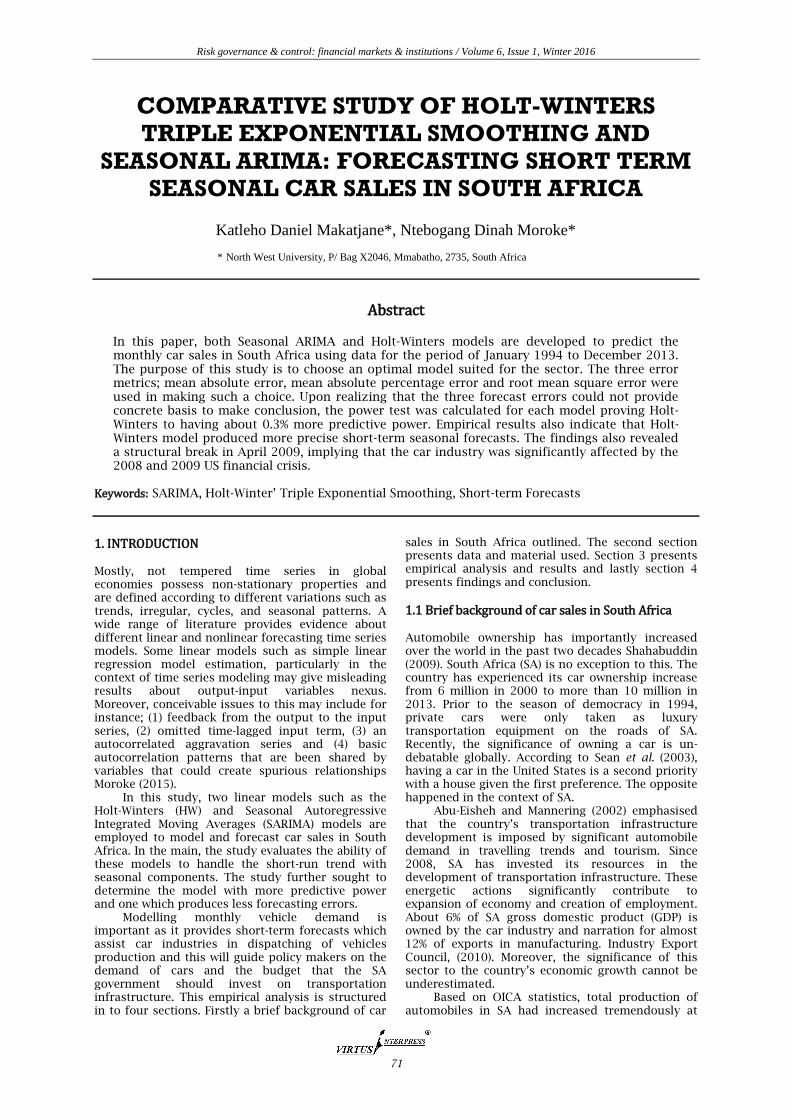
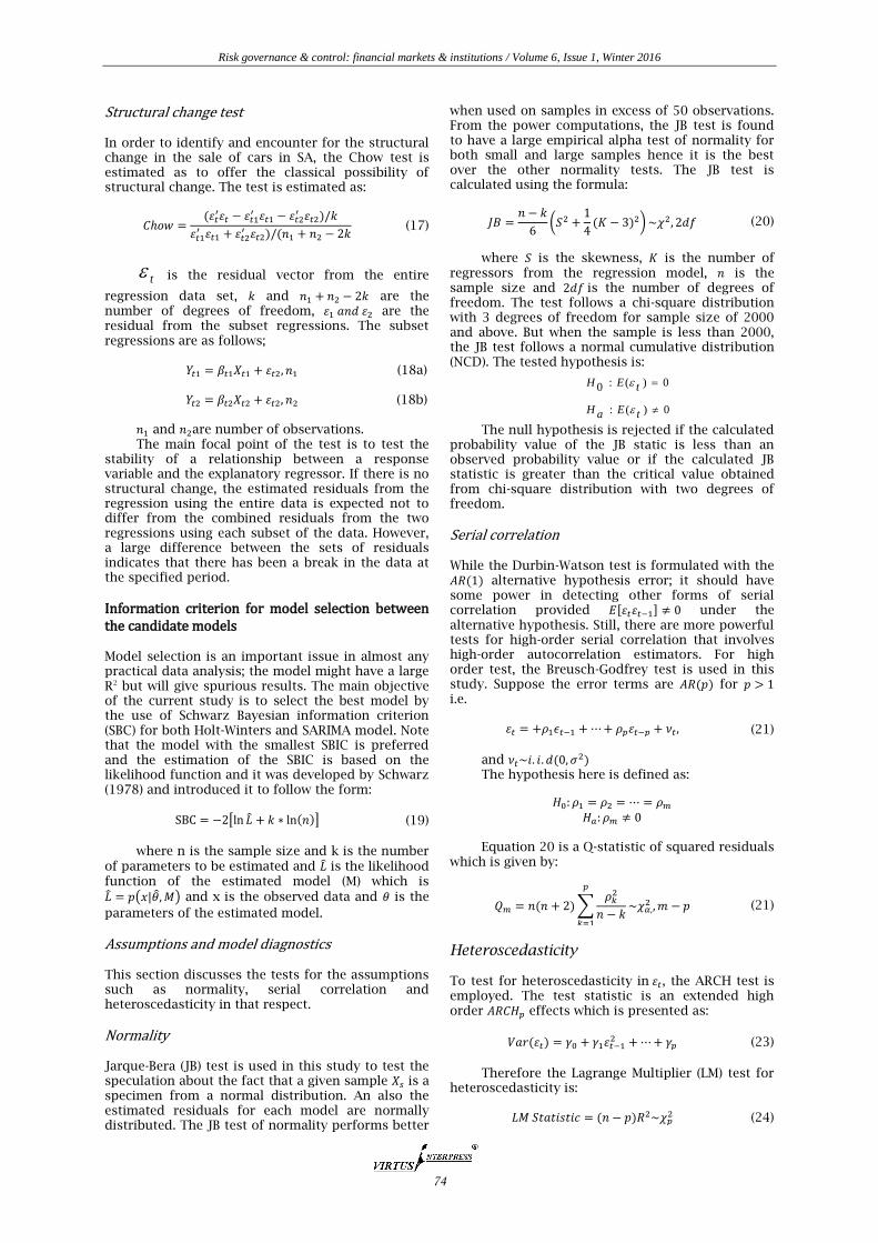
3.2 Structural Break Test In univariate timeseries analysis, the overlay plots are normally adopted to check the behaviour of the data. Figure 1 is the plot of monthly car sales from 1994 to 2013 in SA. The figure shows a roughly increasing seasonal trend. This implies that the series of car sales is nonstationary. Generally, car industry in the country was doing well with some time epochs during some seasons. In the 184th observation, i.e. monthly sales in April 2009, there was a break from the sales of cars in SA as shown by a profound dip. This period marks a numerical drop from 53,000 cars in March to 38,200 cars in April. It should be noted that, most of the countries suffered the spill-over effects of US financial crisis which occured between 2007-2009. These effects started hiting most economies after 2009 and during that time most financial sectors of different countries suffered the effects causing the slowing down in production, people being retrenched and most

industries closing down. SA also suffered economic recession, hence a dip in 2009.

The cause of this intense change is the increase in unemployment and poverty in the whole world which contributed to the decline in aggregate demand. According to Moroke et al. (2014), the 2007-2009 crisis had a colossal effect on economies, with securities exchanges falling, financial institutions caving in and governments been compelled to intercede with bailouts, while trying to put more attention on administrative change. This also brought a significant drop on the economic growths globally. The South African Reserve Bank (SARB) 2010 quarterly report uncovers that South Africa's GDP was 15.3% in 2009. Currently the rate of economic growth in SA is at 2% as per annual bulletin from the SARB.


76

Figure 1. Total Monthly Car Sales

Table 2. Chow structural change test

Test Break Point Num DF Den DF F Value Prob

Chow 184 13 214 4.34 **

Notes *** significant @ 10% ** significant at 5%, *significant at 1%; N not significant

The Chow test in Table 2 supports a significant structural break on the 184th observation associated with April 2009 also vissible in Figure 1. The dummy interaction variable (Dum1) in Table 3 is also statistically siginificant at 5% level of significance.

This implies that this interaction is precipitous with a permanent duration and this means that there is a structural break on April 2009. Chow test also confirms that there was a significant drop of cars sales in SA in April 2009.

Table 3. The Piecewise Regression Parameter Estimates

Variable Coefficient Std. Error t-Statistic Prob.

C 19635.99 1327.861 14.78768 **

T 263.3427 12.50641 21.05661 **

DUM1 -7417.515 2048.603 -3.620767 **


The results in Table 3 indicates that there is a decline of about 7417 in car sales per month. Though SA was not deeply affected by the 2007-2009 financial crisis, the industries within the country were knocked down by the financial overflow. Resources got downgraded, companies were shut down causing unemployment rates to accelerate profusely with the overall diminishing of the country’s economic growth (Moroke et al., 2014).

All of this confirmed Naudé (2009) warnings about the spillover effects of the financial crisis, especially to Africa and those countries dependent on the US for trade.

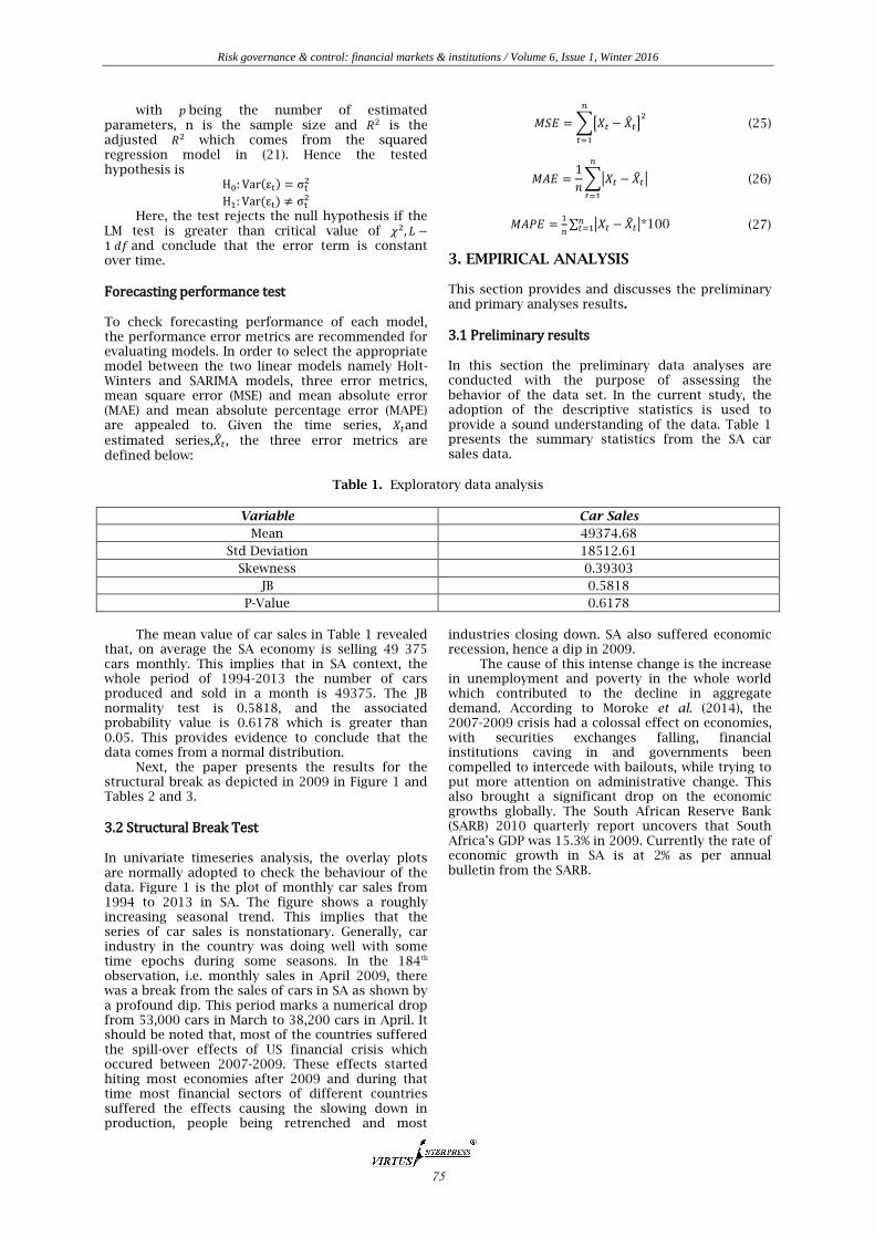
To accommodate the Box-Jenkins methods proposed for this study, the series in Figure 1 is log differenced to help stabilize the properties of time series. The results are shown as Figure 2 and Table 4.

Figure 2. First Seasonal Differencing

10000

20000

30000

40000

50000

60000

70000

80000

90000

0 8 16

24

32

40

48

56

64

72

80

88

96

104

112

120

128

136

144

152

160

168

176

184

192

200

208

216

224

232

240

PLOT Car Sales in South Africa


77

By visual inspection, the partial autocorrelation function (PACF) and autocorrelations function (ACF) of the first log seasonal differencing of the car sales is stationary. The spikes of these functions die

quickly implying that the properties of the series are not time-variant. The statistical test results are presented in Table 4.

Table 4. Augmented Dickey Fuller Test

Type Lags Rho Prob Tau Prob

Zero Mean 0 -299.247 * -20.96 *

1 -636.153 * -17.74 *

2 -509.297 * -10.74 *

3 -589.248 * -8.86 *

Single Mean 0 -299.275 * -20.92 *

1 -636.514 * -17.71 *

2 -510.448 * -10.72 *

3 -593.203 * -8.84 *

Trend 0 -299.283 * -20.87 *

1 -636.665 * -17.67 *

2 -510.382 * -10.69 *

3 -593.202 * -8.82 *


The ADF test confirms that the series is stationary at 5% level of significant at all lags. The findings also show that the model with the three features will produce better forecasts for car sales in SA. Primary data analysis is performed on stationarised data containing the three features and the results are presented in the next sections.

3.3 Holt-Winter’s Exponential Smoothing Results The estimated Holt-Winters model is reported in table 5. Both multiplicative seasonal model with trend and multiplicative seasonal model are estimated. The best model is selected by the use of SBC which then indicates that the Multiplicative seasonal model is the best because the reported SBC is -1163.4 compared to the winter’s model.

Table 5. Holts-Winters Triple Exponential Smoothing Results

_MODEL_ _PARM_ _EST_ _STDERR_ _TVALUE_ _PVALUE_

WINTERS LEVEL 0.49817 0.039425 12.636 0.000

WINTERS TREND 0.001 0.013329 0.075 0.94026

WINTERS SEASON 0.06647 0.029017 2.2909 0.02285

R2

0.94871

SBC

-1160.4

MULTSEASONAL LEVEL 0.5116 0.039604 12.9177 0.000

MULTSEASONAL SEASON 0.06853 0.029842 2.2964 0.022521

R2

0.94816

SBC

-1163.4

�̂�𝑡 = (0.51160)(0.06853)𝑆𝑡 And the associated 𝑅2 = 0.94816 which means the model is significant because 95% of variation in car sales is explained by

time. And, the seasonal factors are reported in table 6 as.

Table 6. The estimated seasonalities

JAN FEB MAR APR MAY JUN

0.98963 1.0011 1.00893 0.98958 1.00128 1.00545

JUL AUG SEP OCT NOV DEC

1.00707 1.0038 0.9979 1.01053 1.00271 0.98287

The results in table 6 implies that throuhgout the whole period of 1994-2013, there were some irregularities that happened within South African car industry. The estimates are not constant throughout the months as dipicted by Table 5. Montgomery et

al. (2015) cleared that this cyclical parttens are even likely to happen in an out-of sample forecasts.


78

3.3.1 Box-Jenkins SARIMA Results Since both SARIMA and Holt-Winters method are capable of capturing the short run seasonalities within the data, with SARIMA models, the first step is to difference the seasonal and non-seasonal series so as to enable the selection of the best model among candidate models. Which is done through the use of the Bayesian Information Criterion (BIC) The model is identified by an automated procedure

which was suggested by Stadnytska et al. (2008). The use of the traditional way of using the PACF and ACF plots is employed by then examining the behavior of the two plots and then select the model based on the number of spikes outside the confidence bend of the plots. And finally model estimation is done through maximum likelihood estimation method. The parameter estimates of the SARIMA model are reported in table 7.

Table 7. Parameter estimates of SARIMA model

Parameter Estimate Standard Error t Value Pr > |t| Lag

MA1,1 0.5138 0.05806 8.85 0.0001 1

AR1,1 0.20235 0.06619 3.06 0.0022 3

AR2,1 -0.39939 0.06264 -6.38 0.0001 12

The estimated model can be written as:

[1 − 0.20235Φ ∗∗∗ (3)(1 + 0.39939Φ ∗∗∗ (12))]𝑋𝑡

= [1 − 0.5138Θ ∗∗ (1)]휀𝑡, and, 휀𝑡~𝑖𝑖𝑑(0,0.12710).

The point estimates of this model are all significant. These outcomes are as per those of the correlational and full limit versatility theory acquired in the preparatory analyses. As Yaffee and

McGee (2000) suggested, the estimates of the model must be less than one to deem them sufficient and significant. Note that the first-order pure seasonal differencing was established to obtain stationary values of the series.

3.3.2 Model diagnostic check

Table 8. Holt-Winters and SARIMA

Holt-Winters

SARIMA

Statistic

Estimate Prob Statistic

Estimate Prob

JB test

2.9655 N JB test

2.7298 N

Godfrey test

Godfrey test

AR(1) 0.0012 N

AR(1) 0.7622 N

AR(2) 3.0377 N

AR(2) 5.1554 N

AR(3) 11.361 **

AR(3) 5.1562 ***

ARCH test

1.65 N ARCH test

0.002153 N


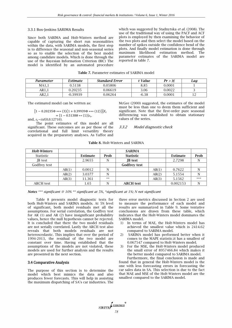
Table 8 presents model diagnostic tests for both Holt-Winters and SARIMA models. At 5% level of significant, both model residuals met all the assumptions. For serial correlation, the Godfrey test for AR (1) and AR (2) have insignificant probability values, hence the null hypothesis cannot be rejected. It is concluded that there the two model residuals are not serially correlated. Lastly the ARCH test also reveals that both models residuals are not heteroscedastic. This implies that over the period of 1994-2013, the residual of the two model are constant over time. Having established that the assumptions of the models are not violated, these models are used for further analysis and the results are presented in the next section.

3.4 Comparative Analysis The purpose of this section is to determine the model which best mimics the data and also produces fewer forecasts. This will help in assisting the maximum dispatching of SA’s car industries. The

three error metrics discussed in Section 2 are used to measure the performance of each model and results are summarized in Table 9. Some tentative conclusions are drawn from these table, which indicates that the Holt-Winters model dominates the SARIMA model. 1) In terms of MAE, the Holt-Winters model has

achieved the smallest value which is 2414.62 compared to SARIMA model.

2) SARIMA model has performed better when it comes to the MAPE statistic.it has a smallest of 0.067547 compared to Holt-Winters model.

3) For the MSE, the Holt-Winters model produced the small error of 8957466.84 which makes it the better model compared to SARIMA model. Furthermore, the final conclusion is made and

found that in general the Holt-Winters model is the one with less forecasting errors in forecasting the car sales data in SA. This selection is due to the fact that MAE and MSE of the Holt-Winters model are the smallest compared to the SARIMA model.


79

Table 9. Performance model selection Criteria

Performance Criteria Holt-winters Model SARIMA Model

MAE_Ratio 2414.62 4288.78

MAPE_Ratio 0.071599 0.067547

MSE_Ratio 8957466.84 27071931.35

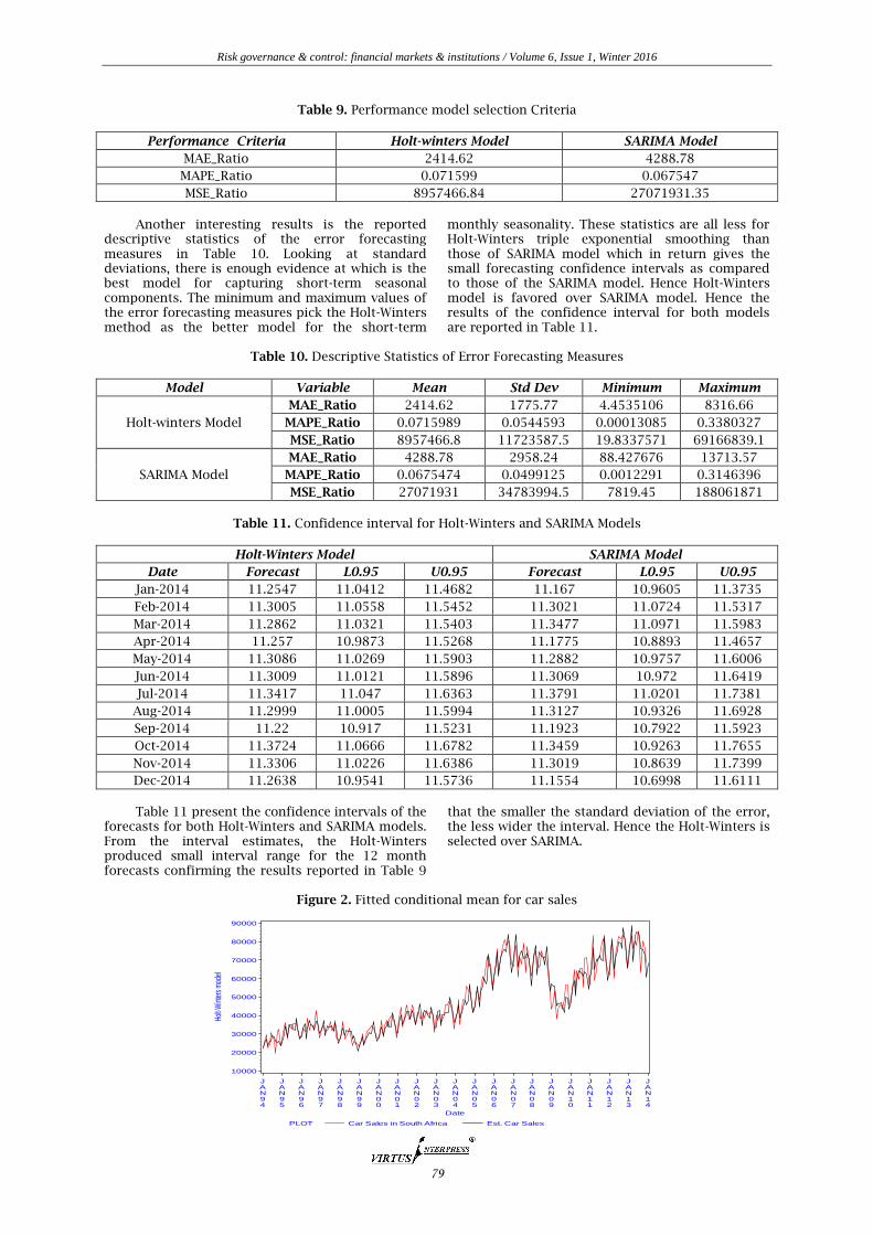
Another interesting results is the reported

descriptive statistics of the error forecasting measures in Table 10. Looking at standard deviations, there is enough evidence at which is the best model for capturing short-term seasonal components. The minimum and maximum values of the error forecasting measures pick the Holt-Winters method as the better model for the short-term

monthly seasonality. These statistics are all less for Holt-Winters triple exponential smoothing than those of SARIMA model which in return gives the small forecasting confidence intervals as compared to those of the SARIMA model. Hence Holt-Winters model is favored over SARIMA model. Hence the results of the confidence interval for both models are reported in Table 11.

Table 10. Descriptive Statistics of Error Forecasting Measures

Model Variable Mean Std Dev Minimum Maximum

Holt-winters Model

MAE_Ratio 2414.62 1775.77 4.4535106 8316.66

MAPE_Ratio 0.0715989 0.0544593 0.00013085 0.3380327

MSE_Ratio 8957466.8 11723587.5 19.8337571 69166839.1

SARIMA Model

MAE_Ratio 4288.78 2958.24 88.427676 13713.57

MAPE_Ratio 0.0675474 0.0499125 0.0012291 0.3146396

MSE_Ratio 27071931 34783994.5 7819.45 188061871

Table 11. Confidence interval for Holt-Winters and SARIMA Models

Holt-Winters Model SARIMA Model

Date Forecast L0.95 U0.95 Forecast L0.95 U0.95

Jan-2014 11.2547 11.0412 11.4682 11.167 10.9605 11.3735

Feb-2014 11.3005 11.0558 11.5452 11.3021 11.0724 11.5317

Mar-2014 11.2862 11.0321 11.5403 11.3477 11.0971 11.5983

Apr-2014 11.257 10.9873 11.5268 11.1775 10.8893 11.4657

May-2014 11.3086 11.0269 11.5903 11.2882 10.9757 11.6006

Jun-2014 11.3009 11.0121 11.5896 11.3069 10.972 11.6419

Jul-2014 11.3417 11.047 11.6363 11.3791 11.0201 11.7381

Aug-2014 11.2999 11.0005 11.5994 11.3127 10.9326 11.6928

Sep-2014 11.22 10.917 11.5231 11.1923 10.7922 11.5923

Oct-2014 11.3724 11.0666 11.6782 11.3459 10.9263 11.7655

Nov-2014 11.3306 11.0226 11.6386 11.3019 10.8639 11.7399

Dec-2014 11.2638 10.9541 11.5736 11.1554 10.6998 11.6111

Table 11 present the confidence intervals of the

forecasts for both Holt-Winters and SARIMA models. From the interval estimates, the Holt-Winters produced small interval range for the 12 month forecasts confirming the results reported in Table 9

that the smaller the standard deviation of the error, the less wider the interval. Hence the Holt-Winters is selected over SARIMA.

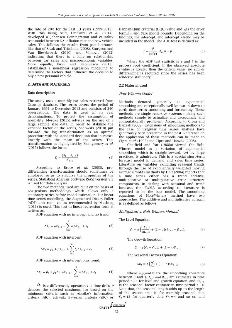
Figure 2. Fitted conditional mean for car sales

Holt-

Win

ters

mod

el

10000

20000

30000

40000

50000

60000

70000

80000

90000

Date

JAN94

JAN95

JAN96

JAN97

JAN98

JAN99

JAN00

JAN01

JAN02

JAN03

JAN04

JAN05

JAN06

JAN07

JAN08

JAN09

JAN10

JAN11

JAN12

JAN13

JAN14

PLOT Car Sales in South Africa Est. Car Sales


80

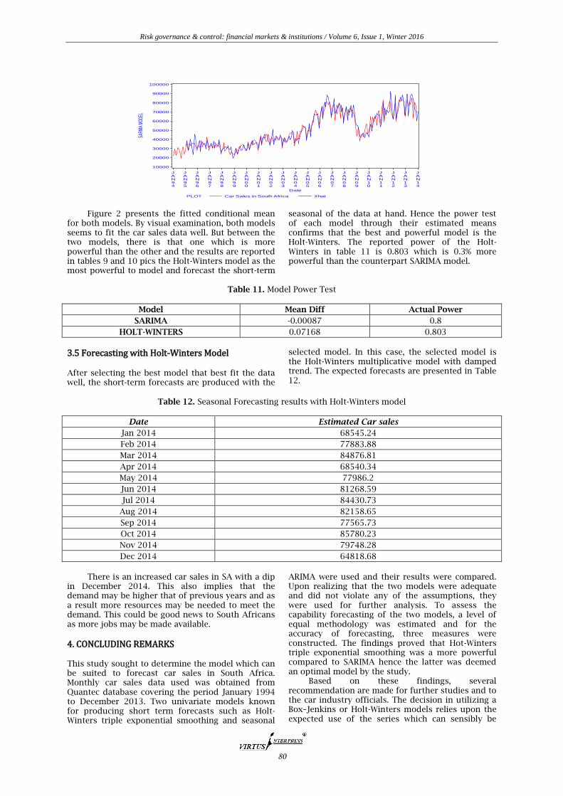
Figure 2 presents the fitted conditional mean for both models. By visual examination, both models seems to fit the car sales data well. But between the two models, there is that one which is more powerful than the other and the results are reported in tables 9 and 10 pics the Holt-Winters model as the most powerful to model and forecast the short-term

seasonal of the data at hand. Hence the power test of each model through their estimated means confirms that the best and powerful model is the Holt-Winters. The reported power of the Holt-Winters in table 11 is 0.803 which is 0.3% more powerful than the counterpart SARIMA model.

Table 11. Model Power Test

Model Mean Diff Actual Power

SARIMA -0.00087 0.8

HOLT-WINTERS 0.07168 0.803

3.5 Forecasting with Holt-Winters Model After selecting the best model that best fit the data well, the short-term forecasts are produced with the

selected model. In this case, the selected model is the Holt-Winters multiplicative model with damped trend. The expected forecasts are presented in Table 12.

Table 12. Seasonal Forecasting results with Holt-Winters model

Date Estimated Car sales

Jan 2014 68545.24

Feb 2014 77883.88

Mar 2014 84876.81

Apr 2014 68540.34

May 2014 77986.2

Jun 2014 81268.59

Jul 2014 84430.73

Aug 2014 82158.65

Sep 2014 77565.73

Oct 2014 85780.23

Nov 2014 79748.28

Dec 2014 64818.68

There is an increased car sales in SA with a dip

in December 2014. This also implies that the demand may be higher that of previous years and as a result more resources may be needed to meet the demand. This could be good news to South Africans as more jobs may be made available.

4. CONCLUDING REMARKS This study sought to determine the model which can be suited to forecast car sales in South Africa. Monthly car sales data used was obtained from Quantec database covering the period January 1994 to December 2013. Two univariate models known for producing short term forecasts such as Holt-Winters triple exponential smoothing and seasonal

ARIMA were used and their results were compared. Upon realizing that the two models were adequate and did not violate any of the assumptions, they were used for further analysis. To assess the capability forecasting of the two models, a level of equal methodology was estimated and for the accuracy of forecasting, three measures were constructed. The findings proved that Hot-Winters triple exponential smoothing was a more powerful compared to SARIMA hence the latter was deemed an optimal model by the study.

Based on these findings, several recommendation are made for further studies and to the car industry officials. The decision in utilizing a Box–Jenkins or Holt-Winters models relies upon the expected use of the series which can sensibly be

SARI

MA M

ODEL

10000

20000

30000

40000

50000

60000

70000

80000

90000

100000

Date

JAN94

JAN95

JAN96

JAN97

JAN98

JAN99

JAN00

JAN01

JAN02

JAN03

JAN04

JAN05

JAN06

JAN07

JAN08

JAN09

JAN10

JAN11

JAN12

JAN13

JAN14

PLOT Car Sales in South Africa Xhat


81

thought continuous, a whiz decision would to be apply a Holt-Winters multiplicative approach. Despite the fact that Box–Jenkins and Holt-Winters models have comparable forecasting ability on car sales data, the latter is more adaptable for managing distinctive data scenarios. The reported quantitative comparison between SARIMA and Holt-Winters is emphatically reliant on the time series and the chosen error measures. Extra assessment of both models was established and found that Holt-Winters has more predictive power than SARIMA. For more interesting studies, a researcher can even include simulated data sets and compare the SARIMA models and Holt-Winters models with other time series techniques, for instance, artificial neural networks. On the side of policy makers, policies regarding the car industries must be re-evaluated. Firstly, national roads should be improved as the forecasts indicated that on monthly bases, the sales of car are increasing over time. This will also bring more income to the South Africa economy through the tourism sector as more people will be visiting SA and as a result GDP will be boosted. Moreover, future economic policy should focus more on new vehicle manufacturing, the sector has the potential to grow and generate employment and more earning to South Africa.

REFERENCES 1. Abu-Eisheh, S.A. & Mannering, F.L. 2002.

Forecasting automobile demand for economies in

transition: A dynamic simultaneous-equation

system approach. Transportation Planning and

Technology, 25 (4):311-331.

2. Box, G.E. & Jenkins, G.M. 1976. Time series analysis,

control, and forecasting. San Francisco, CA: Holden

Day, 3226 (3228):10.

3. Box, G.E., Jenkins, G.M. & Reinsel, G.C. 2011. Time

series analysis: forecasting and control. Vol. 734:

John Wiley & Sons.

4. Bruce, L., Richard, T. & Anne, B. 2005. Forecasting

Time Series and Regression. Thomson Brooks/Cole,

USA.

5. Chatfield, C. & Yar, M. 1988a. Holt-Winters

forecasting: some practical issues. The

Statistician:129-140.

6. Chatfield, C. & Yar, M. 1988b. Holt-Winters

Forecasting: Some Practical Issues. Journal of the

Royal Statistical Society. Series D (The Statistician),

37 (2):129-140.

7. Chifurira, R., Mudhombo, I., Chikobvu, M. &

Dubihlela, D. 2014. The Impact of Inflation on the

Automobile Sales in South Africa. Mediterranean

Journal of Social Sciences, 5 (7):200.

8. Cipra, T. & Hanzák, T. 2008. Exponential smoothing

for irregular time series. Kybernetika, 44 (3):385-

399.

9. Cipra, T., Trujillo, J. & Robio, A. 1995. Holt-Winters

method with missing observations. Management

Science, 41 (1):174-178.

10. DA VEIGA, C.P., DA VEIGA, C.R.P., CATAPAN, A.,

TORTATO, U. & DA SILVA, W.V. 2014. Demand

Forecasting in Food Retail: A Comparison Between

the Holt-Winters and ARIMA Models. WSEAS

Transactions on Business and Economics, 11:608-

614.

11. De Livera, A.M., Hyndman, R.J. & Snyder, R.D. 2011.

Forecasting time series with complex seasonal

patterns using exponential smoothing. Journal of

the American Statistical Association, 106

(496):1513-1527.

12. Ding, Q.Y., Wang, X.F., Zhang, X.Y. & Sun, Z.Q. 2011.

Forecasting traffic volume with space-time ARIMA

model. (In Advanced Materials Research organised

by Trans Tech Publ.

13. Hilas, C.S., Goudos, S.K. & Sahalos, J.N. 2006.

Seasonal decomposition and forecasting of

telecommunication data: A comparative case study.

Technological Forecasting and Social Change, 73

(5):495-509.

14. Holt, C.C. 2004. Forecasting seasonals and trends

by exponentially weighted moving averages.

International Journal of Forecasting, 20 (1):5-10, 1.

15. Hong, W.-C., Dong, Y., Zheng, F. & Wei, S.Y. 2011.

Hybrid evolutionary algorithms in a SVR traffic

flow forecasting model. Applied Mathematics and

Computation, 217 (15):6733-6747.

16. Kamarianakis, Y. & Prastacos, P. 2005. Space–time

modeling of traffic flow. Computers & Geosciences,

31 (2):119-133.

17. Mimovic, P. 2012. Applications of Analytical

Network Process in Forecasting Automobile Sales

of Fiat 500 L. Economic Horizons, 14 (3):169-179.

18. Montgomery, D.C., Jennings, C.L. & Kulahci, M.

2015. Introduction to time series analysis and

forecasting. John Wiley & Sons.

19. Moroke, N.D. 2014. The robustness and accuracy of

Box-Jenkins ARIMA in modeling and forecasting

household debt in South Africa. Journal of

Economics and Behavioral Studies, 6 (9):748.

20. Moroke, N.D., Mukuddem-Petersen, J. & Petersen, M.

2014. A Multivariate Time Series Analysis of

Household Debts during 2007-2009 Financial Crisis

in South Africa: A Vector Error Correction

Approach. Mediterranean Journal of Social

Sciences, 5 (7):107.

21. Mushtaq, R. 2011. Augmented Dickey Fuller Test.

22. Naudé, W. 2009. The financial crisis of 2008 and

the developing countries. UNU-WIDER Discussion

Paper No. 2009/01.

23. Pîrvu, D. & Necşulescu, C. 2013. FUEL

CONSUMPTION: A MAJOR FACTOR INFLUENCING

SALES OF NEW PERSONAL VEHICLES. EVIDENCE

FROM ROMANIAN DATA. Studia Universitatis

Vasile Goldiş, Arad-Seria Ştiinţe Economice, (1):39-

52.

24. Sadowski, E.A. 2010. A Time Series Analysis:

Exploring the Link between Human Activity and

Blood Glucose Fluctuation.

25. Schwarz, G. 1978. Estimating the dimension of a

model. The annals of statistics, 6 (2):461-464.

26. Sean, P.M., Hill, K. & Swiecki, B. 2003. Economic

Contribution of the Automotive Industry to the US

Economy-An Update: A report for the Alliance of

Automobile Manufacturers, Center for Automotive

Research (CAR).

27. Shahabuddin, S. 2009. Forecasting automobile

sales. Management Research News, 32 (7):670-682.


82

28. Sivak, M. & Tsimhoni, O. 2008. Future demand for

new cars in developing countries: going beyond

GDP and population size.

29. Stadnytska, T., Braun, S. & Werner, J. 2008. Model

identification of integrated ARMA processes.

Multivariate Behavioral Research, 43 (1):1-28.

30. Sturgeon, T. & Van Biesebroeck, J. 2010. Effects of

the crisis on the automotive industry in developing

countries: a global value chain perspective. World

Bank Policy Research Working Paper Series.

31. Williams, B.M. & Hoel, L.A. 2003. Modeling and

forecasting vehicular traffic flow as a seasonal

ARIMA process: Theoretical basis and empirical

results. Journal of transportation engineering, 129

(6):664-672.

32. Yaffee, R. & McGee, M. 2000. Introduction to Time Series Analysis and Forecasting with Applications of SAS and SPSS. San Diego. Cal: Academic Press.

Documents

COMPARATIVE STUDY OF HOLT-WINTERS TRIPLE EXPONENTIAL … · TRIPLE EXPONENTIAL SMOOTHING AND SEASONAL ARIMA: FORECASTING SHORT TERM SEASONAL CAR SALES IN SOUTH AFRICA Katleho Daniel