Embed Size (px)
DESCRIPTION
Comparative Study of NAMD and GROMACS. Yanbin Wu, Joonho Lee and Yi Wang Team Project for Phy466 May 11, 2007. Outline. Motivation Simulation Set-up Procedure Result and analysis Conclusion. Motivation (1). NAMD and GROMACS GROMACS: developed in the Netherlands. Fast, free. - PowerPoint PPT Presentation
Citation preview
Comparative Study of NAMD and GROMACS
Yanbin Wu, Joonho Lee and Yi WangTeam Project for Phy466
May 11, 2007
Outline
Motivation
Simulation Set-up
Procedure
Result and analysis
Conclusion
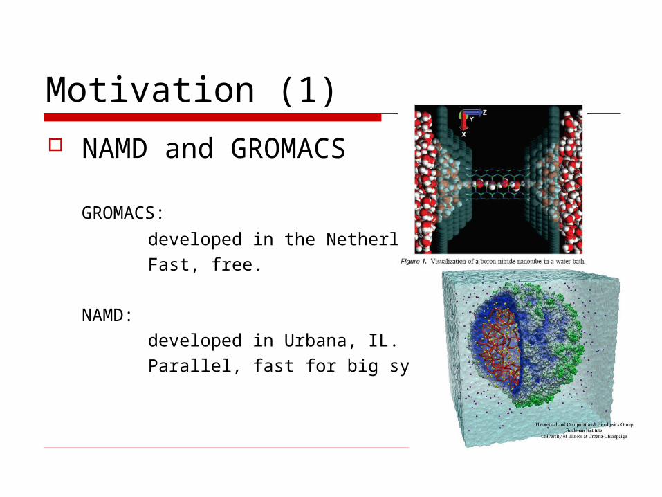
Motivation (1) NAMD and GROMACS
GROMACS:
developed in the Netherlands.Fast, free.
NAMD: developed in Urbana, IL.Parallel, fast for big systems, free.
Motivation (2) Compare two packages
Both are widely used MD packages. Different code implementation in the two
packages may cause different results Generally, one group mainly uses one package
Good chance to compare two packages !!!
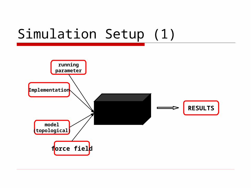
Simulation Setup (1)
SimulationPackage
runningparameter
model(topological)
force field
Implementation
RESULTS
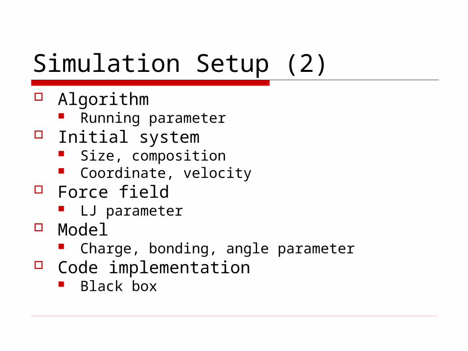
Simulation Setup (2) Algorithm
Running parameter Initial system
Size, composition Coordinate, velocity
Force field LJ parameter
Model Charge, bonding, angle parameter
Code implementation Black box
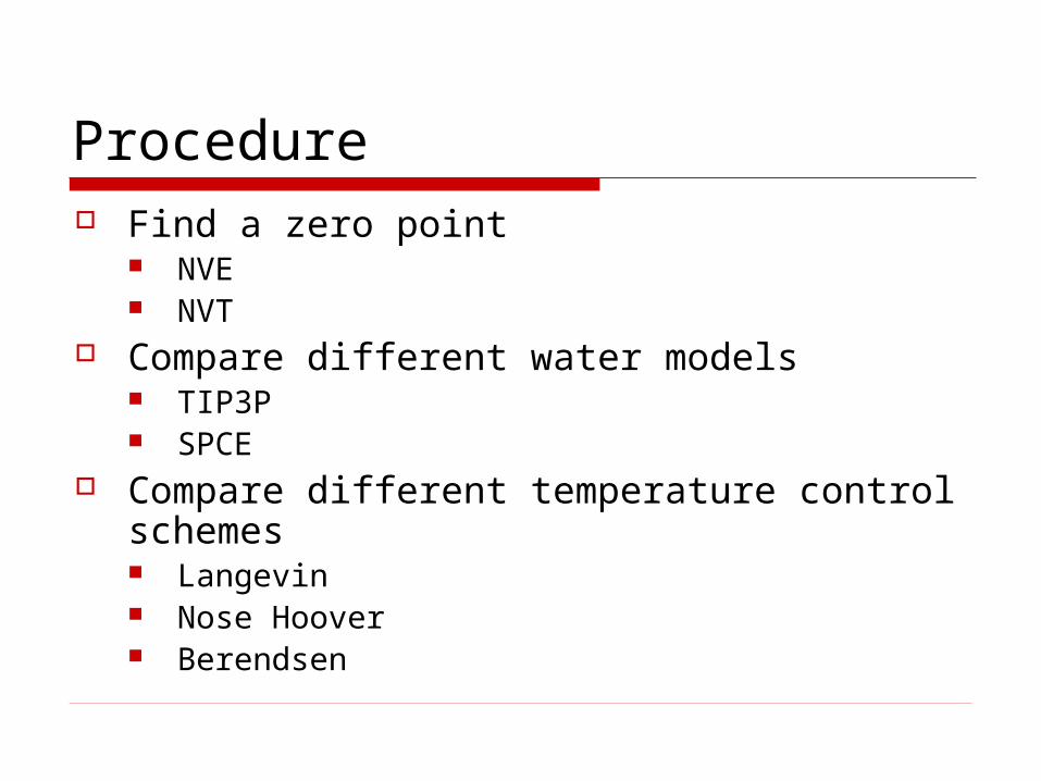
Procedure Find a zero point
NVE NVT
Compare different water models TIP3P SPCE
Compare different temperature control schemes Langevin Nose Hoover Berendsen
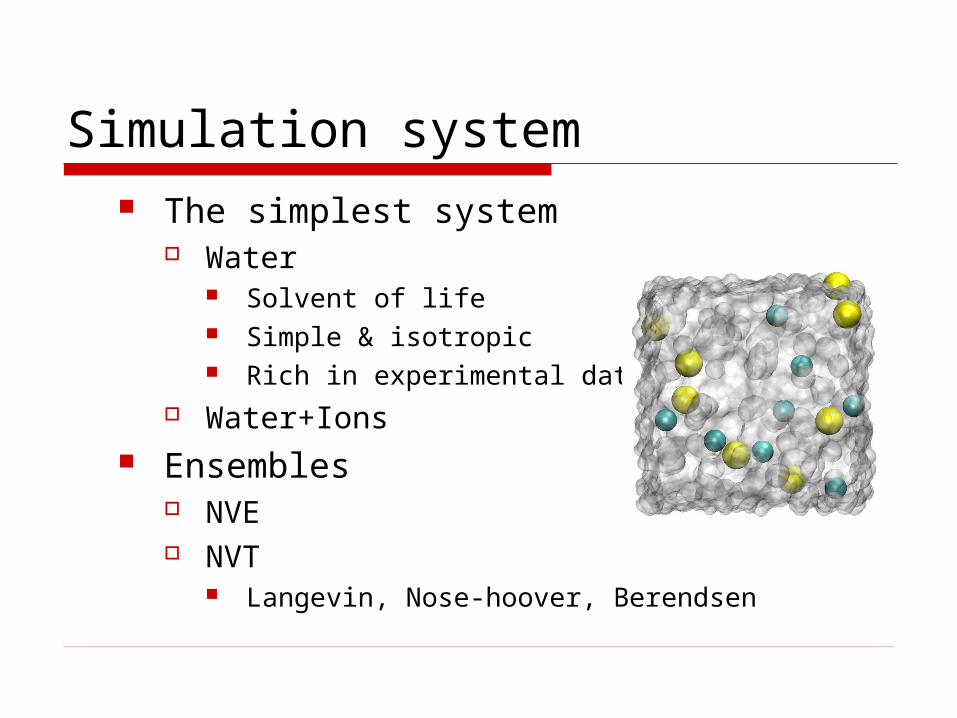
Simulation system The simplest system
Water Solvent of life Simple & isotropic Rich in experimental data
Water+Ions Ensembles
NVE NVT
Langevin, Nose-hoover, Berendsen
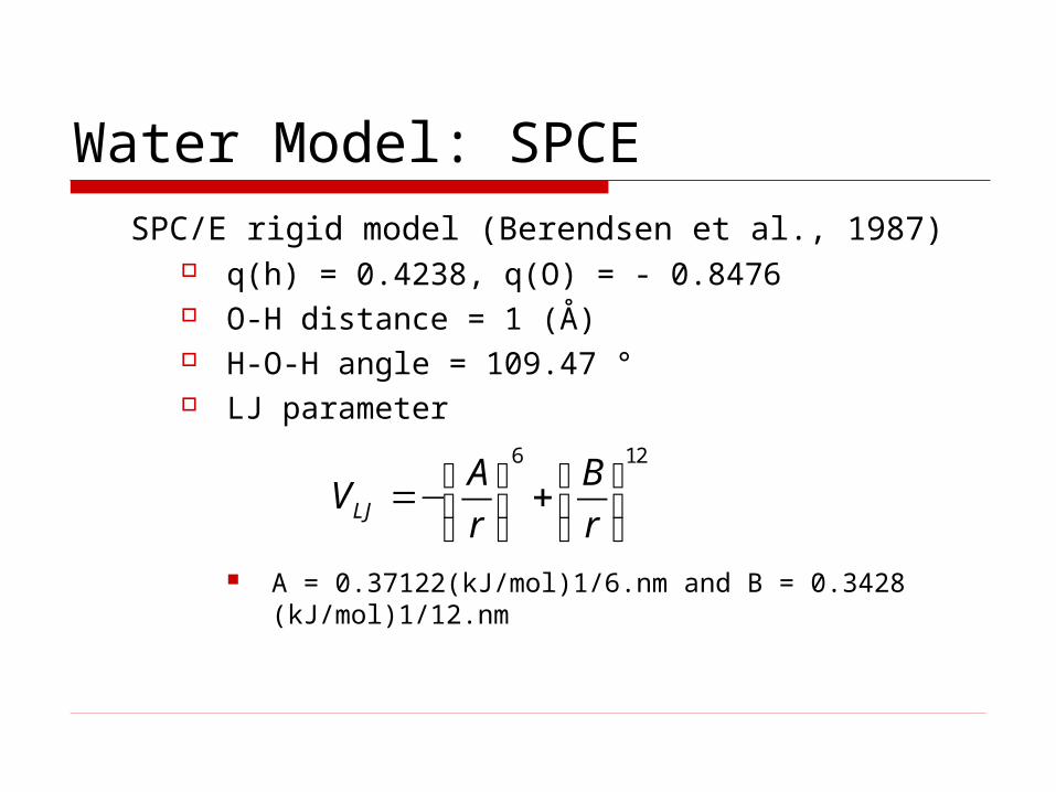
Water Model: SPCESPC/E rigid model (Berendsen et al., 1987)
q(h) = 0.4238, q(O) = - 0.8476 O-H distance = 1 (Å) H-O-H angle = 109.47 ° LJ parameter
A = 0.37122(kJ/mol)1/6.nm and B = 0.3428 (kJ/mol)1/12.nm
6 12
LJ
A BV
r r⎛ ⎞ ⎛ ⎞=− +⎜ ⎟ ⎜ ⎟⎝ ⎠ ⎝ ⎠
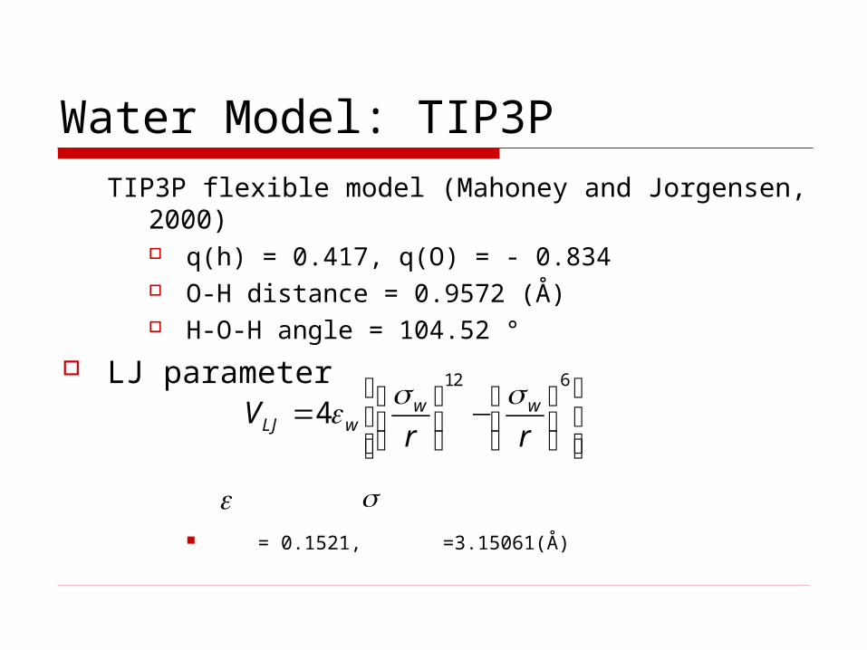
Water Model: TIP3PTIP3P flexible model (Mahoney and Jorgensen, 2000)
q(h) = 0.417, q(O) = - 0.834 O-H distance = 0.9572 (Å) H-O-H angle = 104.52 °
LJ parameter
= 0.1521, =3.15061(Å)
12 6
4 w wLJ wV
r r
σ σε⎡ ⎤⎛ ⎞ ⎛ ⎞= −⎢ ⎥⎜ ⎟ ⎜ ⎟⎝ ⎠ ⎝ ⎠⎢ ⎥⎣ ⎦
ε σ
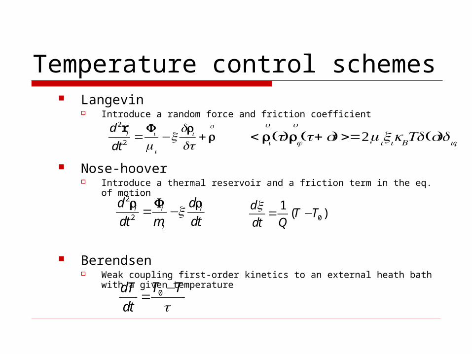
Temperature control schemes Langevin
Introduce a random force and friction coefficient
Nose-hoover Introduce a thermal reservoir and a friction term in the eq. of motion
Berendsen Weak coupling first-order kinetics to an external heath bath with a given
temperature
0T TdT
dt τ−
=
2
2i i i
i
d d
dt m dtξ= −
r F r0
1( )
dT T
dt Q
ξ= −
d 2ri
dt2=
Fi
mi
−ξdri
dt+ r
o
< ri
o
(t)r j
o
(t+ s) >=2miξikBTδ(s)δ ij
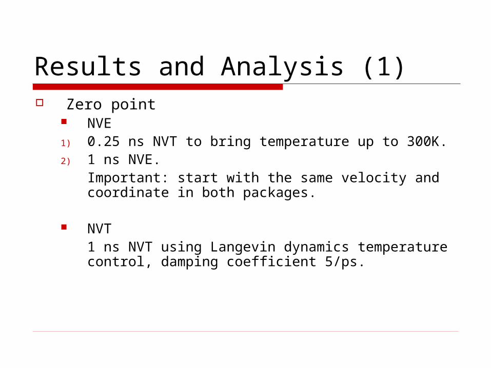
Results and Analysis (1) Zero point
NVE1) 0.25 ns NVT to bring temperature up to 300K.2) 1 ns NVE.
Important: start with the same velocity and coordinate in both packages.
NVT1 ns NVT using Langevin dynamics temperature control, damping coefficient 5/ps.
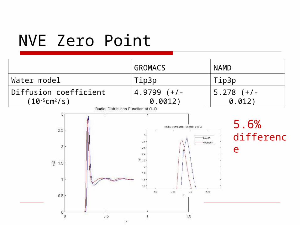
NVE Zero Point
GROMACS NAMD
Water model Tip3p Tip3p
Diffusion coefficient (10-5cm2/s) 4.9799 (+/- 0.0012) 5.278 (+/-0.012)
5.6%difference
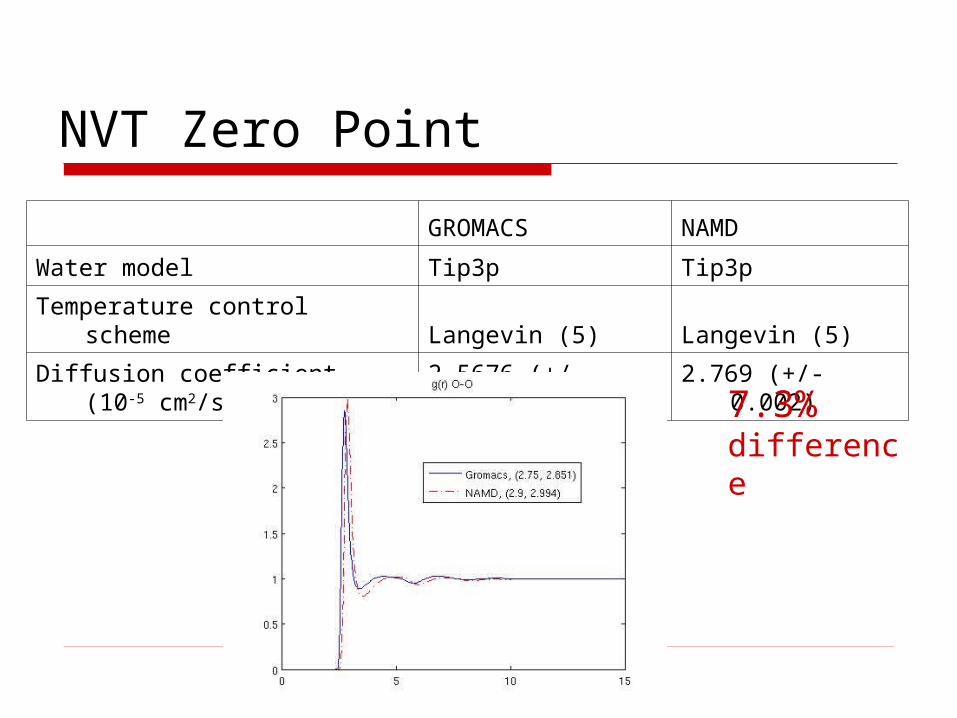
NVT Zero Point
GROMACS NAMD
Water model Tip3p Tip3p
Temperature control scheme Langevin (5) Langevin (5)
Diffusion coefficient (10-5 cm2/s) 2.5676 (+/-0.00009) 2.769 (+/-0.002)
7.3%difference
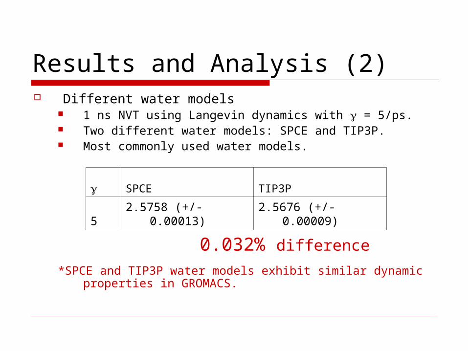
Results and Analysis (2) Different water models
1 ns NVT using Langevin dynamics with = 5/ps. Two different water models: SPCE and TIP3P. Most commonly used water models.
*SPCE and TIP3P water models exhibit similar dynamic properties in GROMACS.
SPCE TIP3P
5 2.5758 (+/- 0.00013) 2.5676 (+/-0.00009)
0.032% difference
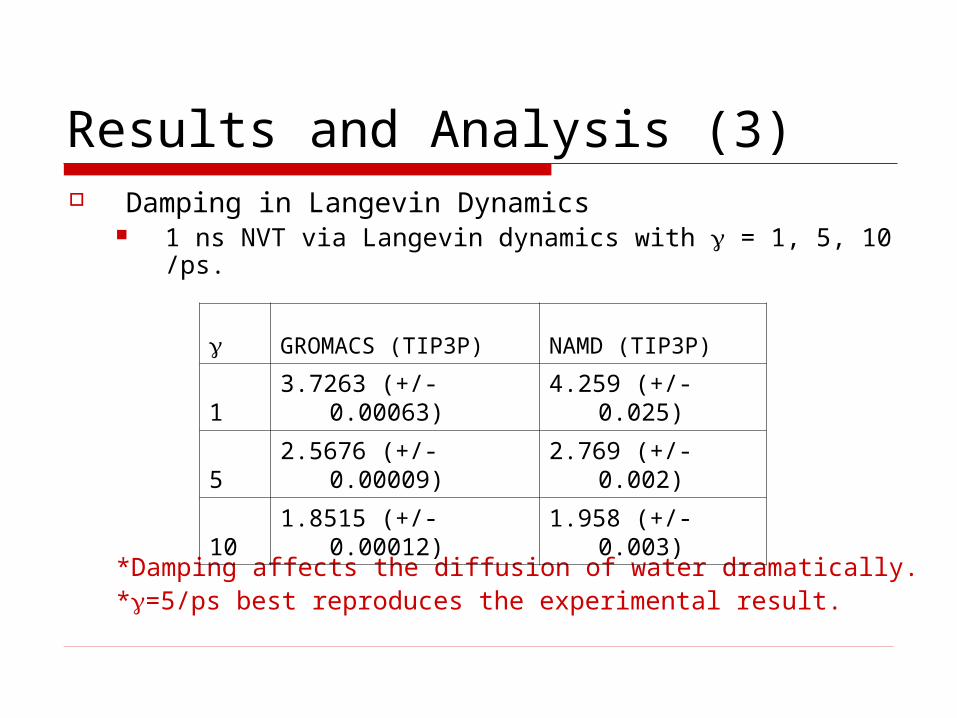
Results and Analysis (3) Damping in Langevin Dynamics
1 ns NVT via Langevin dynamics with = 1, 5, 10 /ps.
*Damping affects the diffusion of water dramatically.*=5/ps best reproduces the experimental result.
GROMACS (TIP3P) NAMD (TIP3P)
1 3.7263 (+/-0.00063) 4.259 (+/-0.025)
5 2.5676 (+/-0.00009) 2.769 (+/-0.002)
10 1.8515 (+/- 0.00012) 1.958 (+/-0.003)
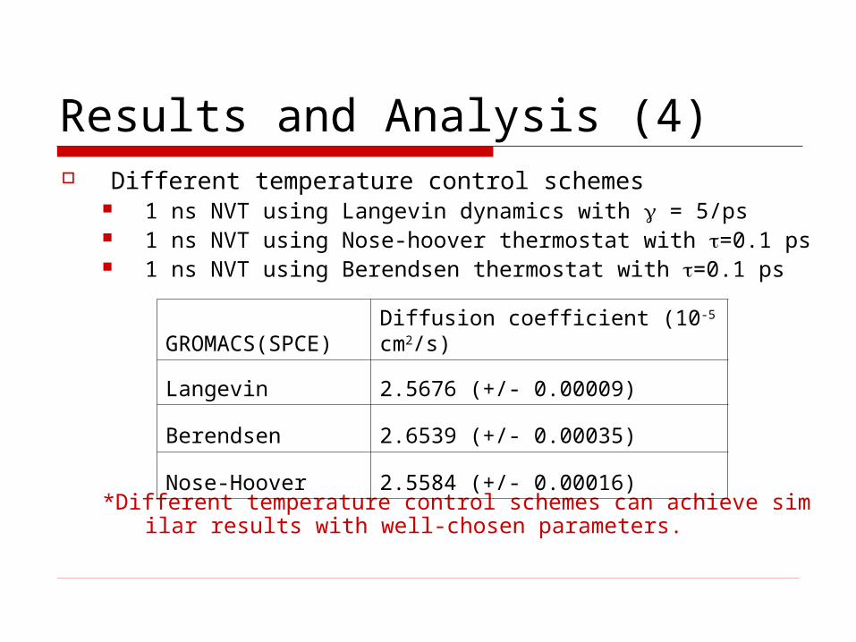
Results and Analysis (4) Different temperature control schemes
1 ns NVT using Langevin dynamics with = 5/ps 1 ns NVT using Nose-hoover thermostat with τ=0.1 ps 1 ns NVT using Berendsen thermostat with τ=0.1 ps
*Different temperature control schemes can achieve similar results with well-chosen parameters.
GROMACS(SPCE) Diffusion coefficient (10-5 cm2/s)
Langevin 2.5676 (+/- 0.00009)
Berendsen 2.6539 (+/- 0.00035)
Nose-Hoover 2.5584 (+/- 0.00016)
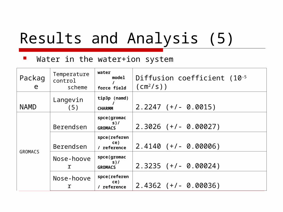
Results and Analysis (5) Water in the water+ion system
PackageTemperature control scheme
water model /force field Diffusion coefficient (10-5 (cm2/s))
NAMD Langevin (5)tip3p (namd) /CHARMM 2.2247 (+/- 0.0015)
GROMACS
Berendsenspce(gromacs)/GROMACS 2.3026 (+/- 0.00027)
Berendsenspce(reference)/ reference 2.4140 (+/- 0.00006)
Nose-hooverspce(gromacs)/GROMACS 2.3235 (+/- 0.00024)
Nose-hooverspce(reference)/ reference 2.4362 (+/- 0.00036)
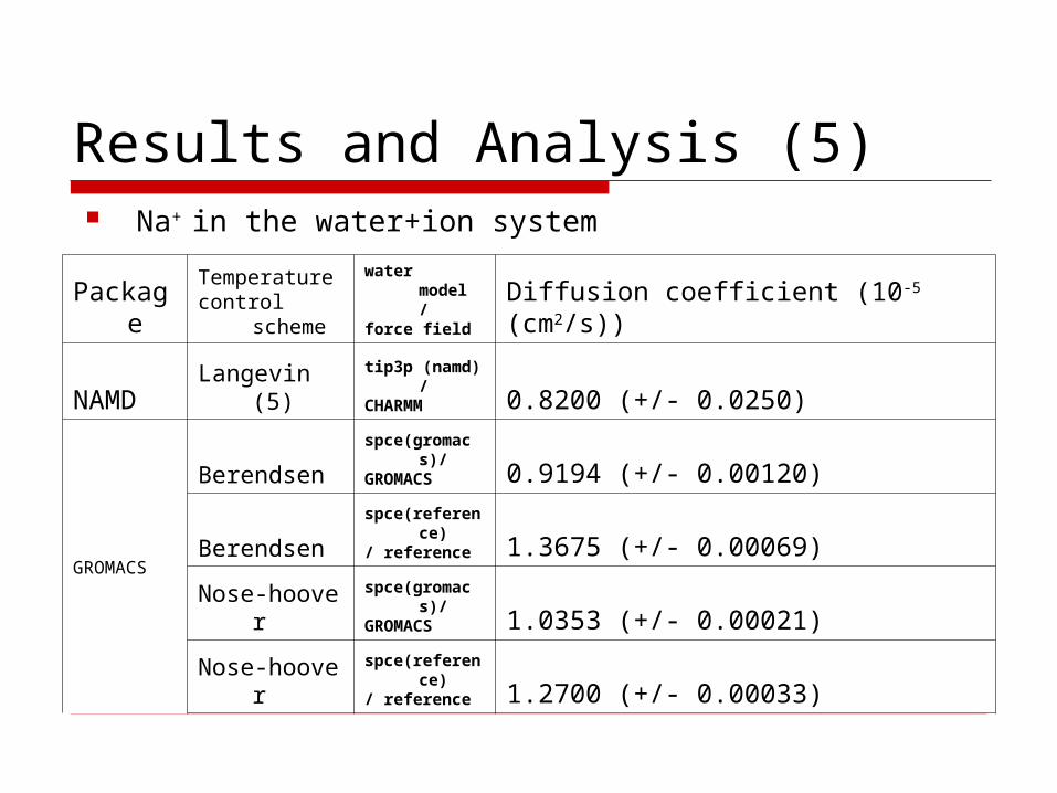
Na+ in the water+ion system
Results and Analysis (5)
PackageTemperature control scheme
water model /force field Diffusion coefficient (10-5 (cm2/s))
NAMD Langevin (5)tip3p (namd) /CHARMM 0.8200 (+/- 0.0250)
GROMACS
Berendsenspce(gromacs)/GROMACS 0.9194 (+/- 0.00120)
Berendsenspce(reference)/ reference 1.3675 (+/- 0.00069)
Nose-hooverspce(gromacs)/GROMACS 1.0353 (+/- 0.00021)
Nose-hooverspce(reference)/ reference 1.2700 (+/- 0.00033)
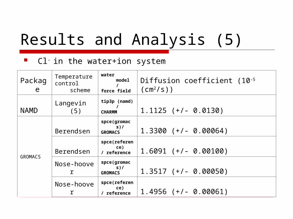
Cl- in the water+ion system
Results and Analysis (5)
PackageTemperature control scheme
water model /force field Diffusion coefficient (10-5 (cm2/s))
NAMD Langevin (5)tip3p (namd) /CHARMM 1.1125 (+/- 0.0130)
GROMACS
Berendsenspce(gromacs)/GROMACS 1.3300 (+/- 0.00064)
Berendsenspce(reference)/ reference 1.6091 (+/- 0.00100)
Nose-hooverspce(gromacs)/GROMACS 1.3517 (+/- 0.00050)
Nose-hooverspce(reference)/ reference 1.4956 (+/- 0.00061)
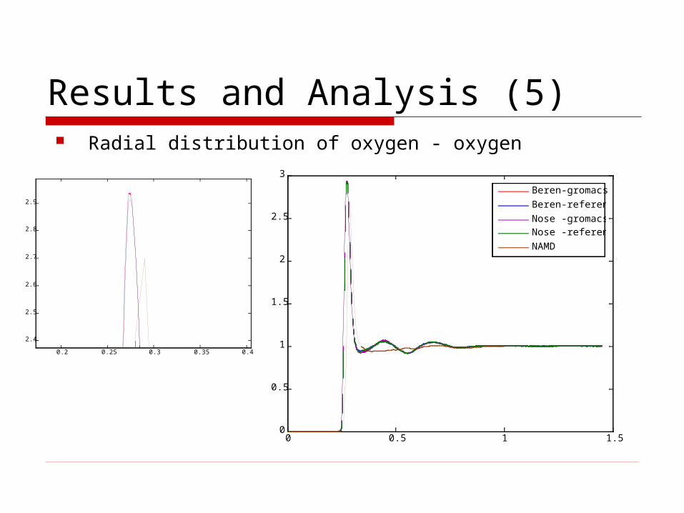
Results and Analysis (5) Radial distribution of oxygen - oxygen
0 0.5 1 1.50
0.5
1
1.5
2
2.5
3
r(nm)
g(r)
oxygen-oxygen
Beren-gromacs
Beren-reference
Nose -gromacsNose -reference
NAMD
0.2 0.25 0.3 0.35 0.4
2.4
2.5
2.6
2.7
2.8
2.9
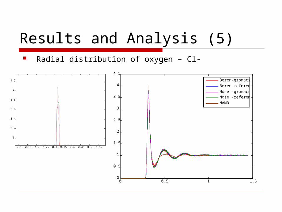
Radial distribution of oxygen – Cl-
Results and Analysis (5)
0 0.5 1 1.50
0.5
1
1.5
2
2.5
3
3.5
4
4.5
r(nm)
g(r)
oxygen - Cl-
Beren-gromacs
Beren-reference
Nose -gromacsNose -reference
NAMD
0.1 0.15 0.2 0.25 0.3 0.35 0.4 0.45 0.5 0.55
3
3.2
3.4
3.6
3.8
4
4.2
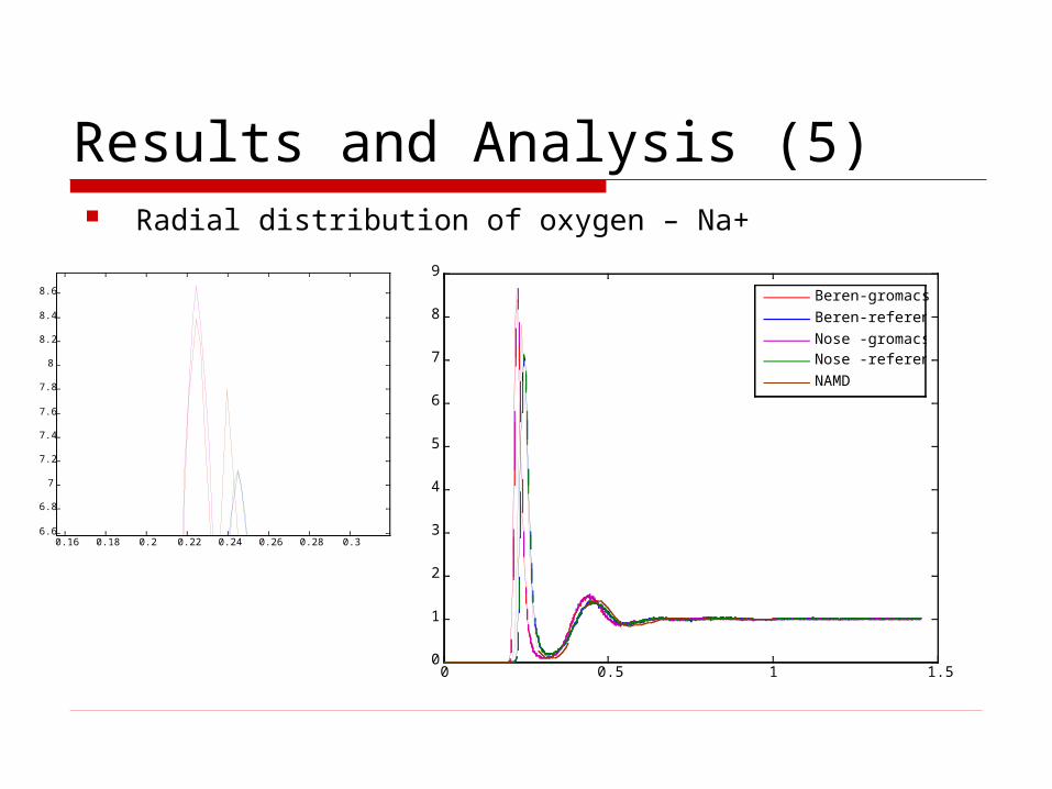
Radial distribution of oxygen – Na+
Results and Analysis (5)
0 0.5 1 1.50
1
2
3
4
5
6
7
8
9
r(nm)
g(r)
oxygen - Na+
Beren-gromacs
Beren-reference
Nose -gromacsNose -reference
NAMD
0.16 0.18 0.2 0.22 0.24 0.26 0.28 0.36.6
6.8
7
7.2
7.4
7.6
7.8
8
8.2
8.4
8.6
Conclusion The two packages GROMACS and NAMD produce similar
results (within tolerance) using the same set of parameters.
Damping coefficient affects the dynamics significantly and has to be chosen with caution.
Different temperature control schemes may generate similar dynamic properties.
Two different water models, SPCE and TIP3P were compared and only minor difference was observed regarding the diffusion of water.
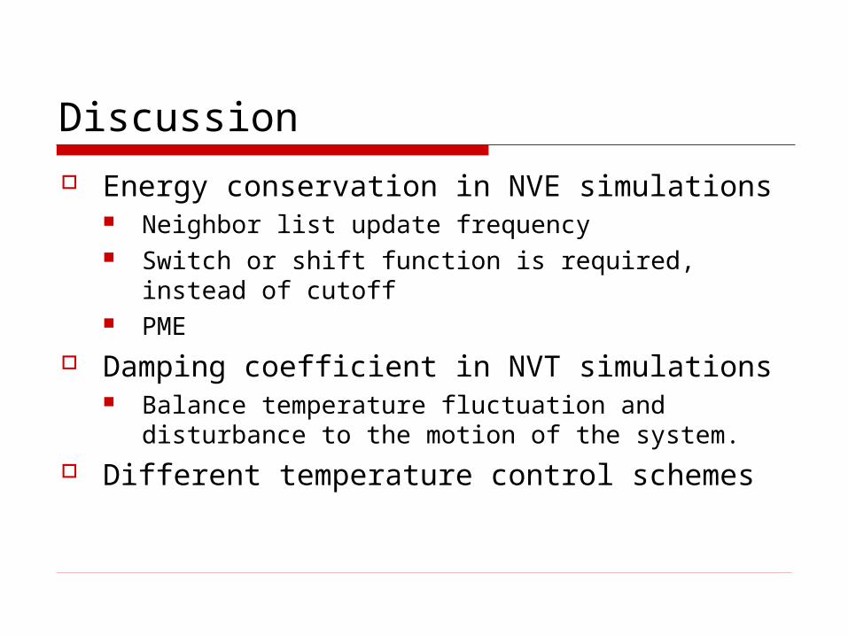
Discussion
Energy conservation in NVE simulations Neighbor list update frequency Switch or shift function is required, instead of
cutoff PME
Damping coefficient in NVT simulations Balance temperature fluctuation and disturbance
to the motion of the system. Different temperature control schemes
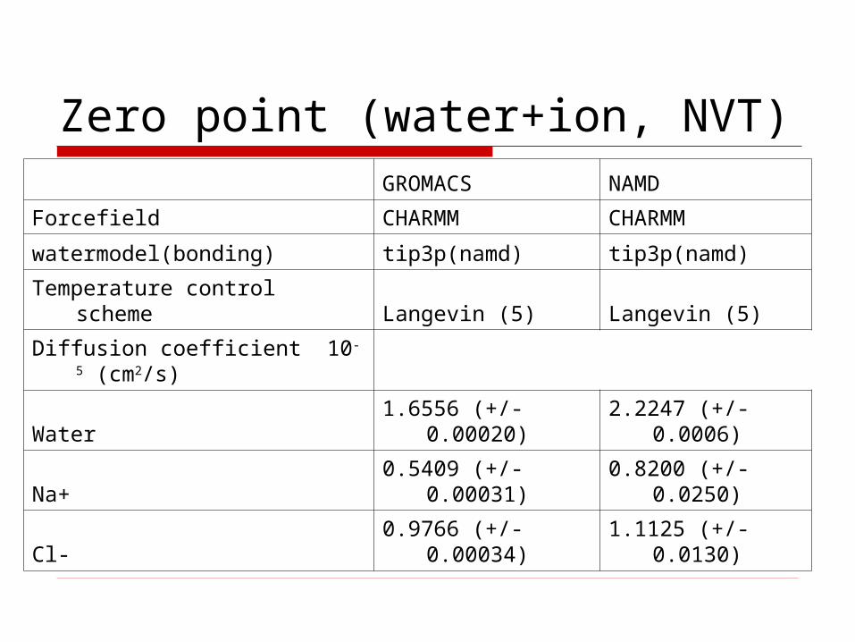
Zero point (water+ion, NVT)GROMACS NAMD
Forcefield CHARMM CHARMM
watermodel(bonding) tip3p(namd) tip3p(namd)
Temperature control scheme Langevin (5) Langevin (5)
Diffusion coefficient 10-5 (cm2/s)
Water 1.6556 (+/-0.00020) 2.2247 (+/-0.0006)
Na+ 0.5409 (+/-0.00031) 0.8200 (+/-0.0250)
Cl- 0.9766 (+/-0.00034) 1.1125 (+/-0.0130)
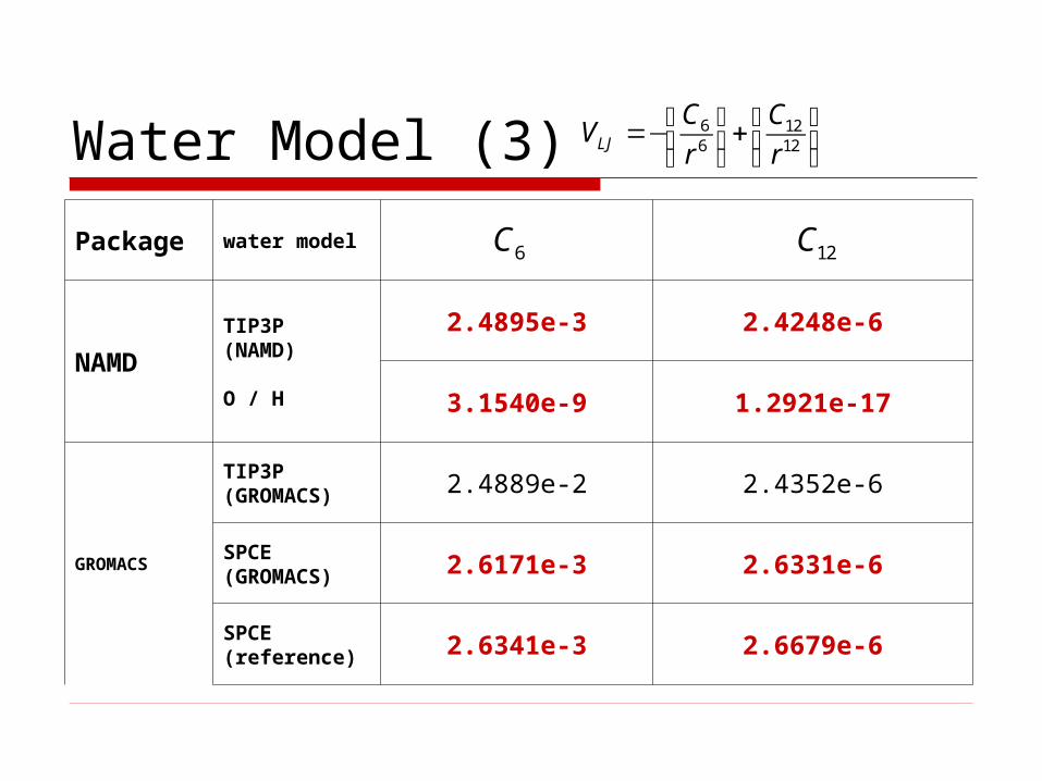
Water Model (3)
Package water model
NAMD
TIP3P(NAMD)
O / H
2.4895e-3 2.4248e-6
3.1540e-9 1.2921e-17
GROMACS
TIP3P(GROMACS) 2.4889e-2 2.4352e-6
SPCE(GROMACS) 2.6171e-3 2.6331e-6
SPCE(reference) 2.6341e-3 2.6679e-6
6C 12C
6 126 12LJ
C CV
r r⎛ ⎞ ⎛ ⎞=− +⎜ ⎟⎜ ⎟
⎝ ⎠⎝ ⎠
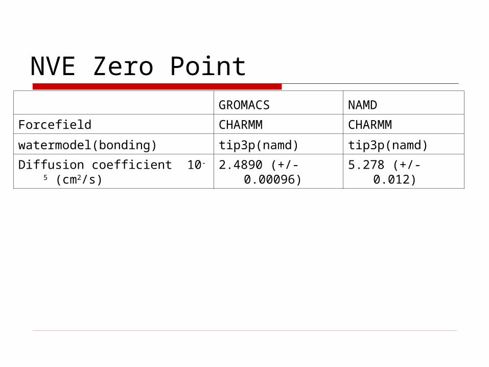
NVE Zero PointGROMACS NAMD
Forcefield CHARMM CHARMM
watermodel(bonding) tip3p(namd) tip3p(namd)
Diffusion coefficient 10-5 (cm2/s) 2.4890 (+/-0.00096) 5.278 (+/-0.012)


![arXiv:1712.03641v2 [physics.comp-ph] 31 Dec 2017 · ... P.R. China and CAEP Software Center for High Performance ... Gromacs [27] and NAMD [28], and path-integral MD ... R ij z ij](https://img.pdfslide.net/doc/110x75/5abfdd327f8b9aca388b4d6f/arxiv171203641v2-31-dec-2017-pr-china-and-caep-software-center-for-high.jpg)