Embed Size (px)
Citation preview

Comparative Study of Pressure Drop Model Equations for Fluid Flow in Pipes
DOI: 10.13140/RG.2.2.12070.55367
Comparative Study of Pressure Drop Model Equations for Fluid Flow in Pipes
Ayoola Idris Fadeyi, B.Sc., M.Sc., MIIAS
Journal of Functional Education; Fall 2020, Volume 4, No. 4, 53-89

1
RESEARCH ARTICLE
Comparative Study of Pressure Drop Model Equations for Fluid Flow in Pipes
Fadeyi, Ayoola Idris, B.Sc., M.Sc., MIIAS
Project Associate
International Institute for African Scholars (IIAS)
Fayetteville, North Carolina
United States of America

2
Abstract
Pressure loss calculation is a very important step in the pipeline design process. As fluid flows
through a pipeline some pressure losses occur. These pressure losses are generally a result of
viscous losses or dissipation. It is very important to know the pressure loss in a pipeline
especially for cases in which the pipe is long. Pressure losses could also be caused by the
presence of pipe fittings such as valves and bends in the pipeline.
In this thesis, the different equations available for the calculation of pressure loss in liquid line
(oil, gas,)and two-phase (gas- oil, oil- water)fluid lines are discussed. The Weymouth,
Panhandle A, Panhandle B and, Spitzglass equations are used to predict gas pressure loss. The
modified Bernoulli/Fanning equation, Hazen-Williams and an empirical equation developed by
Osisanya (2001) are used to predict pressure loss in liquid lines. The two phase gas- oil pressure
loss calculation is carried out using an equation from the American Petroleum Institute (API)
recommended practices and the Lockhart-Martinelli and Chisholm correlations while the two
phase oil- water pressure loss was determined from three friction factor equations, Haaland,
Nikrudase and Blasius.
The gas equations are observed to give varying results depending on the flow rate, pressure and
pipe diameter. The liquid (oil and water) equations gave similar results with the accuracy of the
results increasing with the pipeline diameter. The two-phase pressure loss prediction provides a
good match with the data in the textbook for both the API and Lockhart-Martinelli methods.
In general, the gas equations give similar results for small diameter, low flow rate and low
pressure problems. The liquid equations give more accurate results for larger diameter pipelines.
The gas- oil mixture equations gave results that match the published data while the results
obtained for the oil- water mixture were compared with one another.
3
INTRODUCTION
Background of Study
In the petroleum industry, transportation of the produced oil and gas from the wellhead to the
production facilities as well as to the end-users (consumers) is a very important part of the
production operations. The transportation can either occur in single phase or two phase and
sometimes multiphase. The most common and safest means of transporting the oil and gas from
the wells to the consumers is through pipelines. Pipeline is used to transport the fluids from the
wellhead through different pieces of equipment taking into consideration the pressure
requirements of the producer and customer.
It is highly desirable in pipeline design to be able to accurately predict this phase inversion point
for the flowing oil-water system, since the pressure drop in the pipeline could greatly differ
between an oil-in-water and a water-in-oil systems.
The basic steps in the pipeline design process are calculating the change in pressure along the
pipeline, the line size, pressure rating, and selecting the pipe material. The piping material
chosen is dependent on the properties of fluid to be transported, type of flow expected in the line,
and the operating temperatures and pressures.
A number of pipelines are used depending on the function of the lines. Below is a general
description of pipelines in the oil and gas industry.
a) Injection lines: Pipelines injecting water/steam/polymer/gas into the wells to improve the lift
of fluids from the wells.
b) Flow lines: Pipelines from the well head to the nearest processing facility carrying the well
fluids.
c) Trunk lines/ Inter field lines: Pipelines between two processing facilities or from pig trap to
pig trap or from one block valve station to another processing facility.
d) Gathering lines: One or more segmental pipelines forming a network and connected from the
well heads to processing facilities.
e) Subsea pipelines: Pipelines connecting the offshore production platforms to on-shore
processing facilities.
f) Export lines / Loading lines: Pipelines carrying the hydrocarbons from the processing facility
to the loading or export point.
g) Transmission pipelines: These are pipelines that are used to transport natural gas (methane)
over several kilometers at the pressure of say 100bar
A thorough knowledge of relevant flow equations is very important for calculating pressure drop
of the pipeline as these affect the economics of pipeline transportation. All the equations used in
pipeline design require an understanding of the basic principles of flow regimes, Reynolds
number (to indicate whether flow is laminar or turbulent), Bernoulli’s theorem, Moody friction
factor and a general knowledge of the energy equations. As gas flows through a pipeline, the
total energy contained in the gas is made up of energy due to velocity, pressure, and elevation.
Modified Bernoulli’s equation based upon conservation of energy, connects these components of
energy for the flowing oil and gas between two points.

4
Problem Description
Pipeline transportation is a very important part of the oil and gas industry and it is important to
have a fast and efficient way of calculating the size and pressure requirements of the pipeline to
use in transporting the fluids (oil and gas mixture). The aim of this study is to evaluate the
accuracy of pipeline pressure loss equations and develop a software program using visual basic
with Microsoft excel to ease the calculation of the pressure and size requirements of a pipeline
for single phase(oil, water and gas) flow and two phase (gas- oil, oil- water) flow. There are
numerous equations available for calculating the pressure drop across the pipeline for single
phase and two-phase flows. Based on the review of the equations, appropriate ones for each of
the phases will be selected.
Aims and objective of study
The major objectives of this study are as follows:
1. To evaluate available equations for pipeline calculations and to determine the most suitable
equations for transportation of oil, water, gas and gas- oil, oil- water mixtures.
2. To write a visual basic program to ease the calculation of the pressure drop in the pipeline and
to size pipelines.
3. To validate the calculation with field data as necessary.
These objectives will be achieved by doing a thorough review of the equations available for the
transportation of gases, oil and oil mixtures (gas- oil, oil- water) mixtures in pipelines and
comparing the predictions of these equations with measured data.
Chapter 2: THEORETICAL BACKGROUND LITERATURE REVIEW
Literature Review
A thorough understanding of some basic principles and equations is required for the calculation
of pressure loss across a pipeline. These fundamental principles are used to derive equations for
pressure loss across a pipeline. They include the use of dimensionless groups such as the
Reynolds number and the Moody friction factor, modified Bernoulli’s theorem, Darcy’s equation
and the concept of flow regimes.
Single Phase
a) Liquid Line (Oil, Water) Flow
The Reynolds number Re is a dimensionless number that gives a measure of the ratio of inertial
forces to viscous forces and thus shows the contribution of these forces to fluid flow (Reynolds,
1844). The Reynolds number is an indicator of the flow regime of the flowing fluid. In general,
less than 2100 implies laminar flow, greater than 4000 implies turbulent flow and a number in
between is considered as transitional flow and can be either laminar or turbulent. Laminar flow
occurs when there is little mixing of the flowing fluid, and this means that the fluid flows in
parallel with the pipe wall.
The Bernoulli equation is another essential equation to fluid flow calculations. Bernoulli's
principle states that for an inviscid (non-viscous) flow, an increase in the speed of the fluid
occurs simultaneously with a decrease in pressure or a decrease in the fluid's potential energy.

5
(Bernoulli, 1738).The simplest form of the Bernoulli equation can be used for incompressible
flow.
Darcy’s equation in head loss form is another fundamental equation to fluid flow. It was first
proposed by Darcy and modified by Weisbach in 1845. It related the head loss or pressure loss
due to friction along a given pipe length to the average velocity of the fluid.
The Moody friction factor, credited to Moody (1944) after his study on friction factors for pipe
flow is an important parameter in describing friction losses in pipe and open channel flow. It is
highly dependent on the flow regime which is another reason why the Reynolds number is very
important. The Moody chart relates the friction factor, f, Reynolds number, and relative
roughness for fully developed flow in a circular pipe. It is used to calculate the pressure drop
across the circular pipeline. The Moody chart can be divided into laminar and turbulent regions.
For the laminar flow region, the friction factor is expressed as a function of the Reynolds number
alone while for turbulent flow however, the friction factor is a function of Re and pipe
roughness.
The majority of the material transported in pipelines is in the form of a liquid (crude oil). The
pressure loss for liquid lines (oil and water) can be calculated using a variety of methods all
based on the modified Bernoulli’s equation. A simple empirical equation to calculate the
pressure drop was developed by Osisanya (2001). This equation was developed based on the
pressure recorded between a berth operating platform (BOP) and a single point mooring system
(SPM). This equation was developed in order to select the right pipeline diameter to use to
design a loading pipeline.
In the early stages of natural gas transportation, simple methods were used to calculate the
pressure loss across pipeline due to the low pressure and small diameters of pipeline. As the
industry developed over the last several years, demand for natural gas has increased and the need
for more refined and exact equations to calculate pressure losses in larger-diameter, high-
pressure pipelines with very high velocities and flow rate have been developed.
b) Gas Line
The general flow equation derived from the law of conservation of energy is the foundation of all
equations used to calculate the pressure distribution in a gas pipeline (Katz et al, 1959). The main
difference in the different pipeline equations for gas flow is the specification of the friction
parameter.
Weymouth (1912) derived one of the first equations for the transmission of natural gas in high-
pressure, high-flow rate, and large diameter pipes (Menon, 2005). Brown et al. (1950) modified
the Weymouth equation to include compressibility factor. The compressibility factor is included
in this equation because unlike liquids (oil and water) where the density is constant in the
pipeline, the gas expands or contracts as it flows through the pipe and thus the density varies.
The addition of heat or compressor stations to the pipeline also causes the density to decrease or
increase respectively (Arnold and Stewart. 1986).
Previous studies (Hyman et al. 1976) have shown that the Weymouth equation can give a value
for the pressure loss that is too high especially for large-diameter, low-velocity pipelines. This is
because the friction factor correlation for the Weymouth equation is diameter dependent and is
only useful for 36-in pipeline under fully turbulent flow conditions and is not recommended for
use in calculating pressure loss for new pipelines (Asante, 2000).
The Panhandle A equation was developed in 1940 to be used in large- diameter, long-pipelines
with high-pressure. This equation was initially developed based on data from the Texas

6
Panhandle gas pipeline in Chicago, which operated at 900 psi mostly under turbulent flow
condition (Asante, 2000).
The modified Panhandle equation, usually referred to as the Panhandle B equation, was
developed in 1956 for high flow rates. Both Panhandle equations are dependent on Reynolds
number but the Panhandle B is less dependent than the former because it included implicit values
for pipe roughness for each diameter to which it is applied. The disadvantage of the Panhandle
equation as highlighted by Asante (2000) is that a good estimate of the efficiency factors is
required and this can only be obtained from operating data. This equation is thus not
recommended for planning purposes.
The Spitzglass equation (1912) was originally used in fuel gas piping calculations (Menon.
2005). There are two versions of this equation for low pressures and high pressures but it is
generally used for near-atmospheric pressure lines. A study of this equation by Hyman et al.
(1976) shows that, for pipe diameters over 10 inches, the Spitzglass equation gave misleading
results. This is because the friction factor in this equation is diameter dependent and as the
diameter increases, the friction factor also increases. For fully turbulent flow, the relative
roughness is controlling and so as the diameter increases, the relative roughness decreases. This
is what causes the error in the values obtained for the Spitzglass equation.
There are numerous other equations that have been developed to calculate or estimate pressure
loss for gas flow in pipelines, because of the compressibility of gases. During flow through the
pipeline compressed gas expands depending on the temperature both within and outside the
pipeline. The friction factor and Reynolds number are very important in determining what
equation to use to calculate the pressure loss. This study will compare the results obtained from
the diameter dependent friction factor equations (Spitzglass and Weymouth equations) and the
Reynolds number dependent friction factor equation (Panhandle A and B) for the flow of gas in
pipelines.
Two Phase
a) Gas- Oil Flow
Two-phase gas-oil flow is a complex physical process that occurs extensively in petroleum
industry and other industrial applications. The most important parameters when dealing with gas-
oil flow are pipe geometry, physical properties of the gas and oil such as density and viscosity,
and flow conditions such as velocity, temperature, and pressure (Meng et al. 1999). The
stratified smooth, stratified wavy, intermittent (plug and slug flow), annular and dispersed bubble
flow patterns can be observed in horizontal pipelines. The major problem when calculating the
pressure loss for the flow of gas-oil mixtures is the presence of different flow patterns at different
locations of the same pipeline. As the gas- oil mixture enters the pipeline, the heavier fluid (oil)
tends to flow at the bottom.
Gas- oil flow is common within the wellbore when the fluid is flowing from the reservoir
through the production tubing to the wellhead. Flow from the wellhead to separator is also gas-
oil flow. Some offshore facilities such as ExxonMobil in Nigeria separate the oil, gas, and water
on the platform to know the quantities of each phase present in the produced fluid. The oil and
gas are then combined again and flowed to the onshore terminal. Other companies such as
Chevron, producing in offshore Nigeria, first separate the crude into oil, gas, and water and flow
only oil to the terminal. In both cases, there will be gas entrained in the oil to form a two phase
flow because even when gas removal is attempted, it is never completely removed and so there is
always a significant amount of gas left in the pipeline.

7
Lockhart and Martinelli (1949) proposed a correlation to solve horizontal multiphase flow
problems. The foundation of their solution was in assuming that for a gas-oil system, the
pressure drop is equal to that of one phase as if it were flowing alone in the pipe multiplied by a
factor which was found to be a function of the ratio of the single phase pressure loss of the oil to
the single phase pressure loss of the gas. Numerous other researchers such as Alves (1954),
Baker (1954), Betuzzi et al (1956) tried to improve upon the work done by Lockhart and
Martinelli (Katz et al. 1959). In two-phase gas-oil flow, the pressure drop can be defined as the
sum of the pressure drop due to acceleration, friction, and elevation (Arnold and Stewart. 1986).
Generally, the pressure drop due to acceleration is negligible and the pressure loss due to friction
is much larger than the sum of the equivalent pressure losses for the single phases. This
additional frictional loss is due to the interfacial forces between the gas and oil phases. The
pressure drop due to elevation is also an important factor because of the effect of elevation on oil
holdup and thus the density of the mixture.
The American Petroleum Institute (API RP 14E) recommends an equation to calculate the
pressure loss in gas- oil flow. This equation was developed based on the following assumptions:
(i) ∆P is less that 10% of inlet pressure, (ii) the flow regime is bubble of mist; and (iii) there are
no elevation changes. The equation is also derived from the general equation for isothermal flow.
Sarica and Shoham of the University of Tulsa worked on fluid flow and separation projects for
an industry consortium. Research is being done on different aspects of multiphase flow and
models have been developed for the analysis of multiphase fluid and their design and application
to the petroleum engineering industry (2010).
b) Oil- Water (Liquid- Liquid)
Two phase liquid- liquid pipe flow is defined as the simultaneous flow of two immiscible liquids
in pipes. Oil/water flow in pipes is a common occurrence in petroleum production, especially for
old oil field and for enhanced oil recovery (EOR) with water injection (cold or hot). Moreover,
two-phase liquid- liquid flow is common in the process and petrochemical industries. Although
the accurate prediction of oil- water flow is essential, oil- water flow in pipes has not been
explored as much as gas- liquid (gas- oil) flow. Models developed for gas- liquid systems cannot
be readily used in liquid- liquid ones due to significant differences between them. The oil- water
systems usually have large difference in viscosities, similar densities, and more complex
interfacial chemistry compared to gas/liquid systems.
During the simultaneous flow of oil and water, a number of flow patterns can appear ranging
from fully separated (or stratified) to fully dispersed ones (Lovick & Angeli, 2004). Stratified
flow has received more attention during the past decades because of its low phase velocities and
well-defined interface. On the other hand, fully dispersed flow can be modeled as a single-phase
flow provided that the dispersion effective viscosity is properly estimated. There is limited
information on the intermediate flow patterns, which lie in between stratified and fully dispersed
flows.
A simple two-fluid oil/water pipe flow model was proposed by Zhang and Sarica (2006) as part
of a three-phase unified model. Flat interface was assumed for the stratified oil/water flow. The
transition from stratified flow to dispersed flow is based on the balance between the turbulent
energy of the continuous phase and the surface free energy of the dispersed phase. The inversion
point and effective viscosity of the dispersion are estimated to be using the Brinkman model
(1952).
8
Charles and Redberger (1962) reported on the reduction of pressure gradients in oil pipelines
with water addition. They measured a maximum reduction between 12 and 31% for different
oils. These observations are among the first important studies of oil-water flow in pipes.
Studies of liquid-liquid flow in a pipe often include observation of flow patterns, that is, the
shape and spatial distribution of the two-phase flow within the pipe. But even more important is
the investigation of pressure drop. Today, measurements of the pressure gradient in the different
flow patterns, as well as the development of models are subjected to a lot of research.
Through the years several investigators have contributed to the understanding of liquid-liquid
flow in general and oil-water flow in particular. The inclination angle of the two-phase flow is
one parameter that affects the flow pattern. Pure horizontal flow and pure vertical flow are often
idealized cases. In reality, (gas)/oil/water flow in transport-pipes and wells often have an
inclination angle different from 0 or 90 degrees.
Several models for prediction of pressure drop in liquid-liquid flow exist. Below, the two-fluid
model for stratified flow and the homogeneous model for dispersed flow are presented. Among
others, Brauner and MoalemMaron (1989) and Valle and Kvandal (1995) employed the two-
fluid model for stratified flow on liquid-liquid systems. For dispersed liquid-liquid flow
investigators like Mukherjee et al. (1981) and Valle and Utvik (1997) used the homogeneous
model.
For the purpose of this study the friction factor governing the liquid- liquid flow is of most
interest to us. The friction factors of both phases are calculated using the equation developed by
Haaland (1983).Similarly the friction coefficient can be determined by inserting the mixture
Reynolds number into for instance the Blasius equation. Nikrudase equation is also considered.
Theoretical background
This section deals with the theoretical background of the fundamental principles, concepts and
equations used in pipeline pressure loss calculations. The chapter will review the theories used
for the development of the equations for Single phase flow, (oil, water, and gas) and two-phase
flow (gas-oil and oil- water) and how these equations will be applied in the development of the
program to calculate pressure distribution in pipelines.
Single Phase Flow
Reynolds Number and Friction Factor
The Reynolds number Re is a dimensionless number that gives a measure of the ratio of inertial
forces to viscous forces and thus shows the contribution of these forces to fluid flow. It is
expressed in the general form as:
𝑅𝑒 =𝐼𝑛𝑒𝑟𝑡𝑖𝑎𝑙 𝐹𝑜𝑟𝑐𝑒𝑠
𝑉𝑖𝑠𝑐𝑜𝑢𝑠 𝐹𝑜𝑟𝑐𝑒𝑠=
(𝜌𝑉2
𝐷)
(µ𝑉
𝐷2)=
𝜌𝑉𝐷
µ=
𝑉𝐷
𝑣=
𝑄𝐷
𝑣𝐴 2.1
Reynolds Number= 𝑅𝑒 = 𝐷𝑣𝜌/ µ 2.2
Where: Re= Reynolds number
𝐷= internal diameter of pipe- inches
𝑉= Mean fluid velocity- ft/ sec
𝜌= density
µ= viscosity of fluid
𝑣 =kinematic viscosity= µ/ ρ
Q= volumetric flow rate
9
The Reynolds number can be expressed in different forms for liquid and gases. Equations (2.3),
(2.4), and (2.5) give the Reynolds equation in field units for liquid (oil, water) and Equation (2.6)
is for gas flow.
𝑅𝑒 = 7738𝑆𝐺∗𝑑∗𝑉
µ 2.3
𝑅𝑒 = 7738𝑆𝐺∗𝑄𝐿
µ∗𝑑 2.4
𝑅𝑒 = 928𝜌∗𝑑∗𝑉
µ 2.5
𝑅𝑒 = 20100𝑆∗𝑄𝐺
µ∗𝑑 2.6
The Reynolds number is very essential to describing the flow regimes of the flowing fluids and
then used to determine the necessary equations to be used in the calculation of pressure loss. It is
important to know what flow regime the fluid is in before selecting the equation to use to
calculate pressure loss. To solve for problems in transitional flow, the values for transitional flow
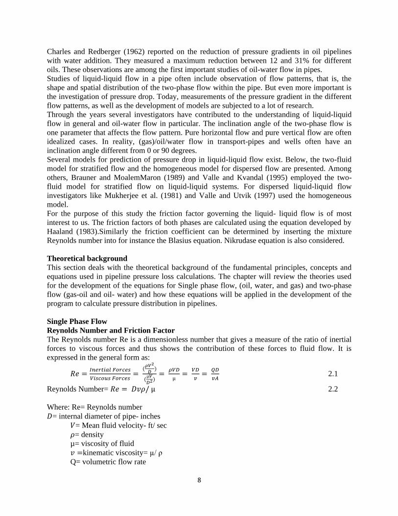
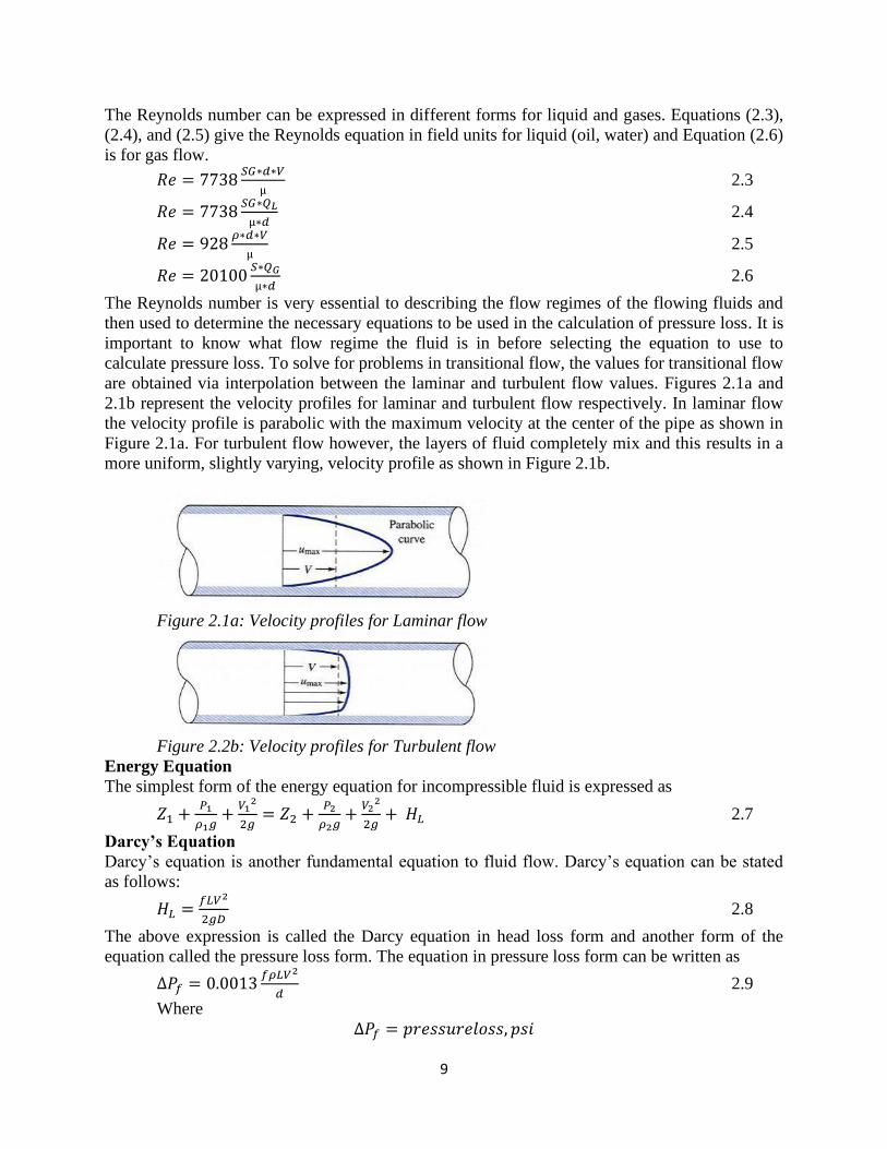
are obtained via interpolation between the laminar and turbulent flow values. Figures 2.1a and
2.1b represent the velocity profiles for laminar and turbulent flow respectively. In laminar flow
the velocity profile is parabolic with the maximum velocity at the center of the pipe as shown in
Figure 2.1a. For turbulent flow however, the layers of fluid completely mix and this results in a
more uniform, slightly varying, velocity profile as shown in Figure 2.1b.
Figure 2.1a: Velocity profiles for Laminar flow
Figure 2.2b: Velocity profiles for Turbulent flow
Energy Equation
The simplest form of the energy equation for incompressible fluid is expressed as
𝑍1 +𝑃1
𝜌1𝑔+
𝑉12
2𝑔= 𝑍2 +
𝑃2
𝜌2𝑔+
𝑉22
2𝑔+ 𝐻𝐿 2.7
Darcy’s Equation
Darcy’s equation is another fundamental equation to fluid flow. Darcy’s equation can be stated
as follows:
𝐻𝐿 =𝑓𝐿𝑉2
2𝑔𝐷 2.8
The above expression is called the Darcy equation in head loss form and another form of the
equation called the pressure loss form. The equation in pressure loss form can be written as
∆𝑃𝑓 = 0.0013𝑓𝜌𝐿𝑉2
𝑑 2.9
Where
∆𝑃𝑓 = 𝑝𝑟𝑒𝑠𝑠𝑢𝑟𝑒𝑙𝑜𝑠𝑠, 𝑝𝑠𝑖

10
Liquid Line Oil, water
The same equations were used for both oil and water throughout only in the Hazen Williams
Equation where dimensional consistency was taken into consideration. The majority of the
material transported in pipelines is in the form of oil (crude oil). The pressure drop for oil (water)
lines can be calculated using a variety of methods all based on the energy equation or modified
Bernoulli’s Equation.
a) Bernoulli Equation
The equation for oil flow derived from the pressure loss form of Darcy’s Equation, Eq. (2.8) can
be used for both laminar and turbulent flow with the only difference being in the calculation of
the friction factor.
∆𝑷𝒇 = (𝟏𝟏. 𝟓 ∗ 𝟏𝟎−𝟔)𝒇𝑳𝑸𝑳
𝟐(𝑺𝑮)
𝒅𝟓 2.10
b) Hazen Williams’s Equation
The Hazen-Williams equation can be used to calculate pressure drop (P1-P2) in a liquid line is
𝑸𝑳 = 𝟎. 𝟏𝟒𝟖 ∗ 𝑪𝒉 ∗ 𝒅𝟐.𝟔𝟑 [∆𝑷−∆𝑷𝑬
𝑳∗𝑺𝑮]
.𝟓𝟒
2.11
Ch = Hazen Williams coefficient
∆PE = elevation changes correction, psia
Experiments and experience have shown that the Hazen-Williams equation does not give
reasonable results when the Hazen-Williams coefficient is less than 90. Historical experimental
data shows that C is a strong function of Reynolds number and pipe size and has narrow
applicable ranges for these two values (Liou, 1998).
c) Empirical Equation
Another empirical equation developed by Osisanya (2001) is also available for calculating the
liquid pipeline pressure loss. This equation was developed using actual oilfield data.
∆𝑷𝒇 =𝑸𝑳∗𝑽𝟎.𝟐𝟓𝟑∗𝑺𝑮𝑳
𝟏𝟓𝟔.𝟒∗𝒅𝟒.𝟕𝟒𝟖 2.12
Gas Flow
The general flow equation derived from the law of conservation of energy in the form of
modified Bernoulli’s equation is the foundation of all equations used to calculate the pressure
drop (P1-P2) in a gas. The general isothermal equation for gas expansion can be written as
𝑤2 = [144𝑔𝐴2
Ṽ(fL
D+2 log(
P1P2
))] [
P12−P2
2
P1] 2.13
Assuming that: i) there are no compressors, expanders, or elevation changes i.e. no work is done,
ii) gas is flowing under steady state conditions, and iii) the friction factor is constant as a
function of length. Equation 2.20 can be rewritten in field units as
𝑄𝐺 = 0.199 [𝑑5(P1
2−P22)
𝑍𝑇𝑓𝑓𝐿𝑆] 2.14
The Weymouth, Spitzglass, and Panhandle equations are all modifications of Equation 2.14 in
which the correlations discussed above are used to calculate the friction factor. The pressure drop
will be calculated by subtracting the downstream pressure, P2, from the upstream pressure, P1 for
each of the equation stated below.
∆𝑃 = 𝑃1 − 𝑃2

11
For all the equations used for gas a base temperature, Tb of 60oF is used in deriving the equations
and this differs from the actual flowing temperature of the fluids in the pipeline, Tf.
a) Weymouth Equation
The Weymouth equation is generally applied to short lines within a production facility. In these
lines, the gas velocity is generally low and thus the Re would be most likely low. These lines
also have high-pressures, high-flow rates and large-diameters. The Weymouth equation is
generally used within the production facility where the Reynolds number is expected to be high.
The Weymouth equation in field units is
𝑸 = 𝟒𝟑𝟑. 𝟒𝟓𝑬 (𝑻𝒃
𝑷𝒃) 𝒅𝟐.𝟔𝟔𝟕 ∗ [
𝑷𝟏𝟐−𝑷𝟐
𝟐
𝑮𝑻𝒇𝑳𝒆𝒁]
𝟎.𝟓
2.15
b) Panhandle A Equation
This equation was developed for use in natural gas pipelines for Reynolds numbers ranging from
5 to 11 million. The pipe roughness is not incorporated into this equation. It can be expressed in
field units as
𝑄 = 435.87𝐸 (𝑇𝑏
𝑃𝑏)
1.0788
∗ [𝑃1
2−𝑃22
𝐺0.8539𝑇𝑓𝐿𝑒𝑍]
0.5394
𝑑2.6182 2.16
c) Panhandle B Equation
This is also called the Modified Panhandle equation and is used for large diameter, high pressure
pipelines. It is applicable for fully turbulent flow in the 4 to 40 million Re range. In this range,
the pipe is assumed to be fully rough. In field units, it is expressed as:
The Panhandle B flow equation is given as:
𝑸 = 𝟕𝟑𝟕𝑬 (𝑻𝒃
𝑷𝒃)
𝟏.𝟎𝟐
∗ [𝑷𝟏
𝟐−𝑷𝟐𝟐
𝑮𝟎.𝟗𝟔𝟏𝑻𝒇𝑳𝒆𝒁]
𝟎.𝟓𝟏
𝒅𝟐.𝟓𝟑 2.17
d) Spitzglass Equation
The Spitzglass equation originally developed for use in fuel gas piping calculation is expressed
in field units as:
𝑸 = 𝟕𝟐𝟗. 𝟔𝑬 (𝑻𝒃
𝑷𝒃) ∗ [
𝑷𝟏𝟐−𝑷𝟐
𝟐
𝑮𝑻𝒇𝑳𝒆𝒁(𝟏+𝟑.𝟔
𝒅+ .𝟎𝟑𝒅)
]
𝟎.𝟓
𝒅𝟐.𝟓 2.18
The Spitzglass equation is applicable mostly to pipelines that are at near atmospheric conditions
and is most ideally suited for diameters less than 12 inches.
Two-Phase Flow
Some companies generally like to separate the gas from the oil as it flows out of the wellhead,
while others especially on offshore platforms leave them to flow together. For this reason, two-
phase gas- oil flow pressure drop is important.
2.2.2.1 Gas- Oil Flow
In the case of gas- oil flow, the gas may appear as tiny amounts of small bubbles in the oil. That
kind of flow occurs when there is relatively little gas compared to oil, at the same time as the oil
flows fast enough to create sufficient turbulence to mix the gas into the oil faster than the gas can
rise to the top of the pipe.
There are several flow regimes available in gas- oil flow and Figure 2.2a shows some of these
regimes. As the gas- oil mixture enters the pipeline, the heavier fluid tends to flow at the bottom.

12
Figure 2.2b shows the transition from one flow regime to another.
Figure 2.2a Gas-Oil flow regimes in horizontal pipes
Figure 2.2b. Example of steady-state flow regime map for a horizontal pipe (Mandhane et al.,
1974)
Similar flow regime maps can be drawn for vertical pipes and pipes with uphill or downhill
inclinations. Notice that even though numerous measured and theoretically estimated such maps
are published in literature, and although they can be made dimensionless under certain conditions
(Taitel & Dukler, 1976), no one has succeeded in drawing any general maps valid for all
diameters, inclinations and fluid properties. Therefore, a diagram valid for one particular
situation (one point in one pipeline with one set of fluid data) is of little help when determining
the flow regime for any other data set. That is why we need more general flow regime criteria
rather than measured flow regime maps. For two phase, gas- oil flow, API and Lockhart-
Martinelli Equations are employed.
a) API Two Phase Equation
The American Petroleum Institute (API) recommends the following equation to calculate the
pressure loss in two-phase gas- oil flow. The equation is also derived from the general equation
for isothermal flow.
∆𝑷𝒇 =𝟑.𝟒∗𝟏𝟎−𝟔𝒇𝑳𝑾𝟐
𝝆𝒎𝒅𝟓 2.19
Where
L = length, ft
W = rate of flow of oil and vapour, lbm/hr

13
𝑊 = (3180 ∗ 𝑄𝑔 ∗ 𝑆𝐺𝑔) + (14.6 ∗ 𝑆𝐺𝐿) 2.20
ρm = density of the mixture, lbm/ft3
𝜌𝑚 =(12409∗𝑆𝐺𝐿∗𝑃)+ (2.7∗
𝑄𝑔∗106
𝑄𝐿∗𝑆𝐺𝑔∗𝑃)
(198.7∗𝑃)+(𝑄𝑔∗106
𝑄𝐿∗𝑇∗𝑧)
2.21
d = pipe ID, in
b) Lockhart-Martinelli
Another Approach to solving two-phase problems can be done using the Lockhart-Martinelli
factor and the Total Pressure Gradient. The individual gas and Oil friction factors are calculated
using the friction factor derived from equations developed by Haaland (1983) and Swamee-Jain
(1976).
𝑓 =1.325
[ln((𝜖
3.7𝑑)+(
5.74
𝑅𝑒0.9))]2 2.22
The superficial velocities for the Oil and gas are calculated using equations (2.23) and (2.24)
respectively.
𝑉𝑠𝑙 =𝑄𝐿
𝑑2 ∗ 0.008938 2.23
𝑉𝑠𝑔 =𝑄𝑔
𝑑2 ∗ 2121.32 2.24
The individual Pressure gradients for the Oil phase and pressure phase are calculated using
equations (2.21) and (2.22) respectively.
𝑑𝑃𝑑𝐿𝐿 = 124.8∗𝑆𝐺𝐺∗𝑓𝑔∗𝑣2
𝑠𝑔
𝑑 2.25
𝑑𝑃𝑑𝐿𝐺 = 124.8∗𝑆𝐺𝐿∗𝑓𝑙∗𝑣2
𝑠𝑙
𝑑 2.26
The two phase multipliers are then calculated using the Lockhart-Martinelli factor and equations
for two-phase multipliers developed by Chisholm (1967). The Lockhart-Martinelli factor is
calculated by
𝑥𝑛 = √𝑑𝑃𝑑𝐿𝐿
𝑑𝑃𝑑𝐿𝐺 2.27
The Chisholm Oil two-phase multiplier is calculated using
∅𝐿 = (1 + 18𝑥𝑛−1 + 𝑥𝑛
−2)0.5 2.28
The Chisholm gas two-phase multiplier is calculated using
∅𝐺 = (1 + 18𝑥𝑛1 + 𝑥𝑛
2)0.5 2.29
The total pressure loss is then calculated using equations (2.26) and (2.27) and the values
obtained should be equal. This is then multiplied by the pipeline length and this gives the two-
phase pressure drop.
𝑑𝑃𝑑𝐿𝐿−𝑇𝑜𝑡𝑎𝑙 = 𝑑𝑃𝑑𝐿𝐿 ∗ ∅𝐿2 2.30
𝑑𝑃𝑑𝐿𝐺−𝑇𝑜𝑡𝑎𝑙 = 𝑑𝑃𝑑𝐿𝐺 ∗ ∅𝐺2 2.31
The pressure loss is then calculated using
∆𝑃2−𝑝ℎ𝑎𝑠𝑒 = 𝑑𝑃𝑑𝐿𝑇𝑜𝑡𝑎𝑙 ∗ 𝐿 2.32
2.2.2.2 Oil- Water Flow
Oil/water flow is a common occurrence during production and transportation of petroleum fluids
through pipes. Understanding of oil/water pipe flow behaviors is crucial to many applications

14
including design and operation of flow lines and wells, separation, and interpretation of
production logs.
For the purpose of this study a dispersed fluid flow pattern of the oil- water was considered. The
pressure drop for each of the equations below is calculated using the friction factor. Water was
emphasized at a constant velocity in order to emphasize the in order to emphasize the effect of
water at constant mixture velocity. The values of the friction factor calculated for each of the
equation are substituted into the given
∆𝑃 =𝑄𝜇𝐿𝑑𝑖 𝑓
2𝜋 2.33
a) Haaland Equation: This equation is generally used for all water cuts. The pipe roughness
is assumed to be zero, hence the friction factor 1
√𝑓= −1.8𝑙𝑜𝑔 (
6.9
𝑅𝑒) 2.34
b) Blassius Equation:
𝑓 = 0.312(𝑅𝑒)−0.25
c) Nikrudase Equation
𝑓 = 0.184(𝑅𝑒)−0.20 2.35
𝑅𝑒𝑚 =𝜌𝑚∗𝑑𝑖∗𝑈𝑚
µ𝑚 Standard Units 2.36
The mixture density is modeled by
𝜌𝑚 = 𝜖𝑤𝜌𝑤 + 𝜖𝑜𝜌𝑜 2.37
By further expressing the mixture velocity as:
𝑈𝑚=𝑈𝑠𝑜 + 𝑈𝑠𝑤 2.38
Where 𝑈𝑠𝑜 and 𝑈𝑠𝑤represents the superficial velocity of oil phase and water phase respectively,
that of water is put at a constant velocity.
The phase fractions assuming no slip are given by:
𝜖𝑤 =𝑈𝑠𝑤
𝑈𝑚𝜖𝑜 = 1 − 𝜖𝑤 2.39

15
Table 2.1: Summary of all flow equations used
Single
Phase
Liquid
line(oil,
water)
a) Bernoulli Equation
∆𝑷𝒇 = (𝟏𝟏. 𝟓 ∗ 𝟏𝟎−𝟔)𝒇𝑳𝑸𝑳
𝟐(𝑺𝑮)
𝒅𝟓
b) Hazen Williams’s Equation
∆𝑃𝐻𝑎𝑧𝑒𝑛−𝑊𝑖𝑙𝑙𝑖𝑎𝑚𝑠= .015∗𝑄𝐿
1.85∗𝐿∗5280∗𝑆𝐺𝐿∗62.4
𝑑4.87∗𝐶1.85∗144
for oil
3.4
∆𝑃𝐻𝑎𝑧𝑒𝑛−𝑊𝑖𝑙𝑙𝑖𝑎𝑚𝑠= 0.00208(100
𝐶)1.85(
𝑔𝑝𝑚
𝑑4.87)1.85𝐿
for water
c) Empirical Equation
∆𝑷𝒇 =𝑸𝑳 ∗ 𝑽𝟎.𝟐𝟓𝟑 ∗ 𝑺𝑮𝑳
𝟏𝟓𝟔. 𝟒 ∗ 𝒅𝟒.𝟕𝟒𝟖
Gas
line
a) Weymouth Equation
𝑃2,𝑊𝑒𝑦𝑚𝑜𝑢𝑡ℎ = [𝑃1
2−𝐺𝑇𝑓𝐿𝑒(𝑄𝑔
0.0153𝐸∗𝑑2.667)
𝑒𝑠 ]
0.5
b) Panhandle A Equation
𝑃2,𝑃𝑎𝑛ℎ𝑎𝑛𝑑𝑙𝑒 𝐴
= [𝑃1
2 − 𝐺0.8539𝑇𝑓𝐿𝑒𝑍 (𝑄𝑔
0.0204𝐸∗𝑑2.6182)
𝑒𝑠]
0.5
c) Panhandle A Equation
𝑃2,𝑃𝑎𝑛ℎ𝑎𝑛𝑑𝑙𝑒 𝐵
= [𝑃1
2 − 𝐺0.961𝑇𝑓𝐿𝑒𝑍 (𝑄𝑔
0.0279𝐸∗𝑑2.53)1/0.51
𝑒𝑠]
0.5
d) Splitzglass Equation
𝑃2,𝑆𝑝𝑙𝑖𝑡𝑧𝑔𝑙𝑎𝑠𝑠
= [𝑃1
2 − 𝐺0.961𝑇𝑓𝐿𝑒𝑍 (𝑄𝑔
0.0279𝐸∗𝑑2.53)1/0.51
𝑒𝑠]
0.5
Two
Phase
Gas- oil a) API
∆𝑃 =3.4 ∗ 10−6𝑓𝐿𝑊2
𝜌𝑚𝑑5
Where
𝑊 = (3180 ∗ 𝑄𝑔 ∗ 𝑆) + (14.6 ∗ 𝑆)
𝜌𝑚
=(12409 ∗ 𝑆𝐺𝐿 ∗ 𝑃) + (2.7 ∗
𝑄𝑔∗106
𝑄𝐿∗ 𝑆𝐺𝑔 ∗ 𝑃)
(198.7 ∗ 𝑃) + (𝑄𝑔∗106
𝑄𝐿∗ 𝑇 ∗ 𝑧)
b) Lockhart-Martinelli factor and
Chisholm
𝑓 =1.325
[ln((𝜖
3.7𝑑)+(
5.74
𝑅𝑒0.9))]2
∆𝑃2−𝑝ℎ𝑎𝑠𝑒 = 𝑑𝑃𝑑𝐿𝑇𝑜𝑡𝑎𝑙 ∗ 𝐿
Oil-
water
a) Haaland Equation 1
√𝑓= −1.8𝑙𝑜𝑔 (
6.9
𝑅𝑒)
b) Blassius Equation
𝑓 = 0.312(𝑅𝑒)−0.25 Blasius
c) Nikrudase Equation
𝑓 = 0.184(𝑅𝑒)−0.20 Nikrudase

16
DEVELOPMENT OF THE PIPELINE PRESSURE DROP PROGRAM
Introduction to writing Program Calculator
The aim of the Microsoft Excel visual basic program is to calculate the pressure loss in pipelines
carrying Oil, gas or a gas-Oil mixture. This program was developed using the theories and
fundamental equations discussed in chapter two. This software is designed to aid in the
designing of pipeline systems to operate at specific flow rate, temperature and pressure
conditions. This chapter includes the description and writing of the program calculator. The
program code is executed once the known parameters are entered into the excel spreadsheet. At
the touch of the command button, the program calculates the compressibility factor, z, then the
elevation factor, s, the equivalent length, and the downstream pressure and/or pressure drop. The
first step in designing the program was to rewrite the equations discussed in chapter two in terms
of the Pressure drop or downstream/outlet pressure.
Pressure Drop Calculation (Assumption and Flow Chart)
Single Phase flow
a) Liquid Oil and Water Flow Line
The following assumptions were made in developing the portion of the program for Oil and
water pipelines.
Figure 3.1 shows the flowchart for the calculations for the liquid lines.
1. Base temperature of 60°F or 520°R
2. Base pressure of 1 atmosphere which is equal to 14.73 psia
3. Flowing temperature is constant within the pipeline
4. Oil and water viscosity and density remain constant.
INPUT OIL
PARAMETERS
CALCULATE REYNOLDS NUMBER
AND FRICTION FACTOR
CALCULATE PRESSURE DROP AND
DOWNSTREAM PRESSURE
DISPLAY ΔP AND P2
Liuid Flow rate, Qo, Qw
Flowing Temperature, Tf Upstream Pressure, P1
Pipe Length, L
Pipe diameter, d
Fluid viscosity, μ

17
Figure 3.1: Oil Calculation Flowchart
b) Gas Flow line
For the gas transportation, the Weymouth, Panhandle A, Panhandle B, and Spitzglass equations
will be used. These equations are selected based on the method of calculating the friction factor.
Figure 3.2 shows the flowchart for the gas calculations.
The following assumptions were made in developing the portion of the program for gas
pipelines:
1. Base temperature of 60°F or 520°R
2. Base pressure of 1 atmosphere which is equal to 14.73 psia
3. Efficiency factor, E, the different values of E are as follows
a. 1.0 brand new pipe
b. 0.95 good operating conditions
c. 0.92 for average operating conditions
d. 0.856 unfavourable operating conditions
4. Gas compressibility, z, varies with flowing temperature and upstream pressure
5. Flowing temperature is constant within the pipeline
Figure 3.2: Gas Calculation Flowchart
Two-Phase Pressure Drop Calculation
The following assumptions were made in developing the portion of the program for two phase
mixture pipelines:
a) Gas- Oil
Figure 3.3 shows the sequence of calculation for the gas- oil flow equations.
1. Base temperature of 60°F or 520°R
Flowing Temperature, Tf
Gas Flow rate, QG
Upstream Pressure, P1 INPUT GAS PARAMETERS Pipe Length, L
Pipe diameter, d
Fluid Efficiency, E
CALCULATE COMPRESSIBILITY FACTOR,
ELEVATION FACTOR, EQUIVALENT
LENGTH
CALCULATE PRESSURE DROP AND
DOWNSTREAM PRESSURE
DISPLAY ΔP AND P2

18
2. Base pressure of 1 atmosphere which is equal to 14.73 psia
3. Flowing temperature is constant within the pipeline
4. Oil viscosity and density remain constant.
Figure 3.3: Two-Phase Calculation Flowchart
b) Oil- Water
Figure 3.4 shows the sequence of calculation for the oil- water flow equations.
1. relative viscosity, µ𝑟 constant at 1.847
2. dispersed phase concentration, φ, viscosity equal to 100, 𝜑µ=100= 0.765
3. Base temperature of 60°F or 520°R
4. Base pressure of 1 atmosphere which is equal to 14.73 psia
INPUT TWO-PHASE , GAS-
OIL PARAMETERS
CALCULATE REYNOLDS NUMBER,
COMPRESSIBILITY FACTOR, FRICTION
FACTOR, MIXTURE DENSITY
CALCULATE PRESSURE DROP AND
DOWNSTREAM PRESSURE
DISPLAY ΔP AND P2
Oil Flow rate, QL
Flowing Temperature, Tf
Upstream Pressure, P1
Pipe Length, L
Pipe diameter, d
Fluid Viscosity, μ
Gas Flow rate, QG
Oil Specific Gravity, SGL Gas Specific Gravity, SGG

19
Figure 3.4: Two-Phase oil- water Calculation Flowchart
Equations Used in Program
This program uses simple equations and sub functions typed into the visual basic code to
calculate the Pressure drop for the selected flow type as well as the downstream pressure, P2. The
equations used for the program are discussed below. The results of P2 in psia versus the pipe
length in miles are also displayed. In cases where actual pipeline data was available, the results
are plotted with the data to show how well they correlate.
3.2.1 Single Phase flow
a) Liquid Oil and Water Flow Line
For the oil and water calculations the equations used are:
𝑅𝑒 = 92.1𝑆𝐺𝐿∗𝑄𝐿
𝑑∗𝜇 3.1
𝑓 =1.325
[ln(𝜖
3.7𝑑+
5.7
𝑅𝑒0.9)] 3.2
∆𝑃𝐵𝑒𝑟𝑛𝑜𝑢𝑙𝑙𝑖 = (11.5 ∗ 10−6)𝑓∗𝐿∗5280∗(𝑆𝐺𝐿)∗𝑄𝐿
2
𝑑5 3.3
INPUT TWO-PHASE, OIL-
WATER PARAMETERS
CALCULATE REYNOLDS NUMBER,
COMPRESSIBILITY FACTOR, FRICTION
FACTOR, MIXTURE DENSITY, MIXTURE
VELOCITY, PHASE FRACTION
CALCULATE PRESSURE DROP AND
DOWNSTREAM PRESSURE
DISPLAY ΔP
Pipe Length, L
Pipe diameter, d
Fluid Viscosity, μ
Oil Specific Gravity, SG
Gas Specific Gravity, S
Oil Flow rate, Qm
Flowing Temperature, Tf
Fixed value for superficial velocity of oil,
Uso

20
∆𝑃𝐻𝑎𝑧𝑒𝑛−𝑊𝑖𝑙𝑙𝑖𝑎𝑚𝑠= .015∗𝑄𝐿
1.85∗𝐿∗5280∗𝑆𝐺𝐿∗62.4
𝑑4.87∗𝐶1.85∗144 for oil 3.4
∆𝑃𝐻𝑎𝑧𝑒𝑛−𝑊𝑖𝑙𝑙𝑖𝑎𝑚𝑠= 0.00208(100
𝐶)1.85(
𝑔𝑝𝑚
𝑑4.87)1.85𝐿for water 3.5
∆𝑃𝐸𝑚𝑝𝑖𝑟𝑖𝑐𝑎𝑙 = 𝑄𝐿
1.785∗𝑉0.253∗ 𝑆𝐺𝐿
156.4∗𝑑4.748 3.6
b) Gas Flowline
For gas, the following will be used:
𝑃2,𝑊𝑒𝑦𝑚𝑜𝑢𝑡ℎ = [𝑃1
2−𝐺𝑇𝑓𝐿𝑒(𝑄𝑔
0.0153𝐸∗𝑑2.667)
𝑒𝑠 ]
0.5
3.6
𝑃2,𝑃𝑎𝑛ℎ𝑎𝑛𝑑𝑙𝑒 𝐴 = [𝑃1
2−𝐺0.8539𝑇𝑓𝐿𝑒𝑍(𝑄𝑔
0.0204𝐸∗𝑑2.6182)
𝑒𝑠 ]
0.5
3.7
𝑃2,𝑃𝑎𝑛ℎ𝑎𝑛𝑑𝑙𝑒 𝐵 = [𝑃1
2−𝐺0.961𝑇𝑓𝐿𝑒𝑍(𝑄𝑔
0.0279𝐸∗𝑑2.53)1/0.51
𝑒𝑠 ]
0.5
3.8
𝑃2,𝑆𝑝𝑙𝑖𝑡𝑧𝑔𝑙𝑎𝑠𝑠 = [𝑃1
2−𝐺0.961𝑇𝑓𝐿𝑒𝑍(𝑄𝑔
0.0279𝐸∗𝑑2.53)1/0.51
𝑒𝑠 ]
0.5
3.9
For all equations used in the gas calculation,
∆𝑃 = 𝑃1 − 𝑃2 3.10
Two Phase Calculation Equations
a) Gas- oil
For Two-Phase the API RP 14E equation is used
∆𝑃 =3.4∗10−6𝑓𝐿𝑊2
𝜌𝑚𝑑5 3.11
Where
𝑊 = (3180 ∗ 𝑄𝑔 ∗ 𝑆) + (14.6 ∗ 𝑆𝐺𝐿) 3.11a
𝜌𝑚 =(12409∗ 𝑆𝐺𝐿∗𝑃)+ (2.7∗
𝑄𝑔∗106
𝑄𝐿∗𝑆𝐺𝑔∗𝑃)
(198.7∗𝑃)+(𝑄𝑔∗106
𝑄𝐿∗𝑇∗𝑧)
3.11b
The Lockhart-Martinelli factor and Chisholm correlations developed discussed in chapter two
are also used for the two-phase pressure drop calculations
b) Oil- water
∆𝑃 =𝑄𝜇𝐿𝑑𝑖 𝑓
2𝜋
1
√𝑓= −1.8𝑙𝑜𝑔 (
6.9
𝑅𝑒) Haaland
𝑓 = 0.312(𝑅𝑒)−0.25 Blasius
𝑓 = 0.184(𝑅𝑒)−0.20 Nikrudase
𝑅𝑒𝑚 =𝜌𝑚∗𝑑𝑖∗𝑈𝑚
µ𝑚 Standard Units

21
The mixture density is modeled by
𝜌𝑚 = 𝜖𝑤𝜌𝑤 + 𝜖𝑜𝜌𝑜
By further expressing the mixture velocity as:
𝑈𝑚=𝑈𝑠𝑜 + 𝑈𝑠𝑤
Where 𝑈𝑠𝑜 and 𝑈𝑠𝑤represents the superficial velocity of oil phase and water phase
respectively.
The phase fractions assuming no slip are given by:
𝜖𝑤 =𝑈𝑠𝑤
𝑈𝑚𝜖𝑜 = 1 − 𝜖𝑤

22
PROGRAM VALIDATION AND ANALYIS
Overview
The Program was validated in two stages that is for each of the flow phase. For the single phase,
the first part of the validation was done for the oil lines using data obtained by Osisanya in a
study to develop a simple empirical pipeline fluid flow equation based on actual oilfield data.
Since no field data could be obtained for the water flow line, the pressure drop for Bernoulli’s
equation and Hazen Williams’s equation were compared and the Osisanya empirical equation
which was developed in 2001 for oil flow was put to test, if it will be applicable for water flow.
There were three cases considered in the oil flow and four cases for water flow in this part using
three different pipeline sizes. The second part of the validation was the done for the gas flow
calculation portion of the program using data obtained from ONEOK Technical Services,
Pipelines group. There were four case studies that were used to test the accuracy of the pressure
drop equations for ideal operating conditions. The two-phase flow was validated for gas- oil and
oil- water using different equations and comparison was made among the equations.
Single Phase
Oil flow equation Validation
The oil flow equations were validated using three different cases with different pipe diameters
with the same oil flowing in each pipeline. The data was validated using results obtained by
Osisanya (2001).The actual field data for a 42-inch diameter, 22 mile pipeline is shown in Table
4.1.
Table 4.1: Actual field Pressure data during a typical loading operation
Oil Loading Rates
(Bbl/hr)
ΔP BOP-SPM (psi)
ΔP BOP-SPM
(psi/mile)
ΔP BOP-SPM (psi)
for 1.34 line
45000 204 9 12
56000 308 14 19
60000 359 16 22
The pressure drop is calculated between the Single Point Mooring (SPM) pressure gauge and the
downstream Berth Operating Platform (BOP). The pressure drop values are shown in Table 4.2
and the results per mile of pipeline is also shown. Because field data was only available for the
42-inch pipeline, the oil flow equations were validated with a 36-inch and 24-inch pipeline as
was done with the data in the paper in which the simple empirical equation was developed.
Table 4.2: Pressure drop from actual field data
Oil Loading Rates
(Bbl/hr)
ΔP BOP-SPM (psi)
ΔP BOP-SPM
(psi/mile)
ΔP BOP-SPM (psi)
for 1.34 line
45000 204 9 12
56000 308 14 19
60000 359 16 22
The specific gravity and viscosity of the oil flowing in the pipelines and the internal pipe
roughness of the pipes is given in Table 4.3.
Table 4.3: Common parameters for Oil Flow

23
Parameters
Values
Units
Flow rate, Q 1080000, 1344000, 1440000 BOPD
Specific Gravity (SG)
0.84
Oil Viscosity (μ)
9.84 cP
Pipe Roughness, (ε)
0.00018 inches
Pipe diameter, (d) 42, 36, 24 inches
Length, (L) 1.34, 2.34,3.34 miles
pipe coefficient, (C) 140
kinematic viscosity of oil (V ) 17 (@25oC) cSt
a) Case 1: 42-inch Pipeline
The 42-inch pipeline pressure drop predictions are directly validated using the field data. The
results are shown in Table 4.4. The results obtained for the 42 inch pipeline with an ID of 41-
inches is presented in Tables 4.5 and 4.6. The predictions of the program are very similar to the
results presented in Osisanya (2001). The average deviation for the modified Bernoulli equation
is 3%, the average deviation for the Hazen-Williams equation is 0% and the average deviation
for the Empirical model is 2%. These slight deviations can be neglected for all practical purposes
since most pressure gauges record whole numbers and there are only very few pressure gauges
that record data to more than 1 decimal point. The Hazen-William equation gives the best result
for this large diameter (42-inch) pipeline.
Table 4.4: Program Validation with 42-inch Pipeline Data from Field Data
ΔP
actual
(psi)
ΔP predicted (psi)
% Deviation from actual field data
=[ 𝛥𝑃 𝑎𝑐𝑡𝑢𝑎𝑙 −𝛥𝑃 𝑝𝑟𝑒𝑑𝑖𝑐𝑡𝑒𝑑
𝛥𝑃 𝑎𝑐𝑡𝑢𝑎𝑙] ∗ 100%
Flowrate,
BPD
Bernoulli
Hazen-
Williams
Osisanya
Bernoulli
Hazen-
Williams
Osisanya
1080000 12 11 11 13 8 8 8
1344000 19 16 17 19 16 13 0
1440000 22 18 19 22 18 17 0
Table 4.5: Results obtained from 42-in Oil Line
ΔP (psi) (Osisanya, 2001)
ΔP predicted (psi)
Pipe
Length,
miles
Flow rate,
BPD
Bernoulli
Hazen-
Williams
Empirical
Bernoulli
Hazen-
Williams
Empirical
1.34 1080000
11 11 13 11 11 13
2.34 19 20 22 19 20 23

24
Table 4.6: Deviation of PPDC from Osisanya Results for 42-in
b) Case 2: 36-inch Pipeline
The results obtained for the 36-inch pipeline with an ID of 35.10-inches is shown in Tables 4.7
and 4.8. The results obtained for the program and the Osisanya’s data vary a little more for this
36-in pipeline. The average deviation for the modified Bernoulli equation is 5%, the average
deviation for the Hazen-Williams equation is 0% and the average deviation for the Empirical
model is 0%. The higher deviation for the modified Bernoulli equation can be attributed to the
calculation of the friction factor and pipe fitting losses that are not included in the equation.
Table 4.7: Results obtained for 36-in Oil Line
3.00 24 25 29 24 25 29
1.34
1344000
16 17 19 16 17 19
2.34 28 29 33 28 29 33
3.00 36 37 42 35 38 43
1.34
1440000
18 19 21 18 19 22
2.34 32 33 37 31 33 38
3.00 41 43 47 40 43 48
ΔP predicted (psi)
% Deviation from Osisanya (2001)
Data= [ 𝛥𝑃 𝑂𝑠𝑖𝑠𝑎𝑛𝑦𝑎 −𝛥𝑃 𝑝𝑟𝑒𝑑𝑖𝑐𝑡𝑒𝑑
𝛥𝑃 𝑎𝑐𝑡𝑢𝑎𝑙] ∗
100%
Pipe
Length,
miles
Flow rate,
BPD
Bernoulli
Hazen-
Williams
Empirical
Bernoulli
Hazen-
Williams
Empirical
1.34 1080000 11 11 13 0 0 0
2.34 19 20 23 0 0 5
3.00 24 25 29 4 0 0
1.34 1344000 16 17 19 6 0 0
2.34 28 29 33 4 0 0
3.00 35 38 43 3 0 2
1.34 1440000 18 19 22 6 0 5
2.34 31 33 38 3 0 3
3.00 40 43 48 2 0 2
ΔP (psi) (Osisanya, 2001)
ΔP predicted (psi)
Pipe
Length,
miles
Flow rate,
BPD
Bernoulli
Hazen-
Williams
Empirical
Bernoulli
Hazen-
Williams
Empirical
1.34 1080000 23 24 27 22 24 27
2.34 40 41 47 39 42 47
3.00 52 53 60 50 53 60
1.34 1344000 35 36 39 33 36 39

25
Table 4.8: Deviation of PPDC from Osisanya Results for 36-in
c) Case 3: 24-inch Pipeline
The results obtained for the 24 inch pipeline with an ID of 23.30-inches is shown in Tables 4.9
and 4.10. The average deviation for the modified Bernoulli equation is 18%, the average
deviation for the Hazen-Williams equation is 0% and the average deviation for the Empirical
model is 6%. The predictions from each equation vary significantly. This can also be attributed
to the same reasons for the discrepancies in the 36 inch diameter pipeline. The smaller diameter
of the line makes the effect of the losses and friction factor even more pronounced.
Table 4.9: Results obtained for 24-in oil Line
2.34 61 62 68 58 62 68
3.00 79 80 88 75 80 88
1.34 1440000 40 40 44 38 41 44
2.34 70 71 77 66 71 77
3.00 89 91 99 85 91 99
ΔP predicted (psi)
% Deviation from Osisanya (2001)
Data= [ 𝛥𝑃 𝑂𝑠𝑖𝑠𝑎𝑛𝑦𝑎 −𝛥𝑃 𝑝𝑟𝑒𝑑𝑖𝑐𝑡𝑒𝑑
𝛥𝑃 𝑎𝑐𝑡𝑢𝑎𝑙] ∗
100%
Pipe
Length,
miles
Flow rate,
BPD
Bernoulli
Hazen-
Williams
Empirical
Bernoulli
Hazen-
Williams
Empirical
1.34 1080000 22 24 27 4 0 0
2.34 39 42 47 3 2 0
3.00 50 53 60 4 0 0
1.34 1344000 33 36 39 6 0 0
2.34 58 62 68 5 0 0
3.00 75 80 88 5 0 0
1.34 1440000 38 41 44 5 0 0
2.34 66 71 77 6 0 0
3.00 85 91 99 4 0 0
ΔP (psi) (Osisanya, 2001)
ΔP predicted (psi)
Pipe
Length,
miles
Flow rate,
BPD
Bernoulli
Hazen-
Williams
Empirical
Bernoulli
Hazen-
Williams
Empirical
1.34 1080000 197 175 199 162 175 187
2.34 344 306 347 283 306 326
3.00 441 392 445 362 392 418
1.34 1344000 293 262 291 241 262 274
2.34 512 458 421 421 458 478

26
Table 4.10: Deviation of PPDC from Osisanya Results for 24-in
4.1.2 Water flow: The calculation and program development is still in progress.
a) Case 1: Pipe Size: 10in
Pipe
length(mile)
Flow rate
∆P(Bernoulli) ∆P(Hazen
Williams)
∆P(Empirical)
Hazen
Williams
(gpm)
Bernoulli,
Empirical,
Qw
(bbl/day)
6.0
100 54857.14
12.5
20.0
6.0
200 68571.43
12.5
20.0
6.0
300 82285.71
12.5
20.0
b) Case 2: pipe size: 16in
Pipe Flow rate ∆P(Bernoulli) ∆P(Hazen ∆P(Empirical)
3.00 656 587 540 540 588 613
1.34 1440000 332 298 275 275 300 310
2.34 580 521 480 480 523 542
3.00 743 667 616 616 671 695
ΔP predicted (psi)
% Deviation from Osisanya (2001)
Data= [ 𝛥𝑃 𝑂𝑠𝑖𝑠𝑎𝑛𝑦𝑎 −𝛥𝑃 𝑝𝑟𝑒𝑑𝑖𝑐𝑡𝑒𝑑
𝛥𝑃 𝑎𝑐𝑡𝑢𝑎𝑙] ∗
100%
Pipe
Length,
miles
Flow rate,
BPD
Bernoulli
Hazen-
Williams
Empirical
Bernoulli
Hazen-
Williams
Empirical
1.34 1080000 162 175 187 18 0 6
2.34 283 306 326 18 0 6
3.00 362 392 418 18 0 6
1.34 1344000 241 262 274 18 0 6
2.34 421 458 478 18 0 6
3.00 540 588 613 18 0 6
1.34 1440000 275 300 310 17 1 5
2.34 480 523 542 17 0 5
3.00 616 671 695 17 1 5

27
length(mile) Hazen
Williams
(gpm)
Bernoulli,
Empirical
Qw
(bbl/day)
Williams)
6.0
1600
54857.14 17.774 17.655
12.5 37.03 36.782
20.0 59.25 59.556
6.0
2000
68571.43
26.68
12.5 55.58027
20.0 88.93
6.0 2400 82285.71
12.5
20.0 124.6
c) Case 3: pipe size: 24in
Pipe
length(mile)
Flow rate,
∆P(Bernoulli) ∆P(Hazen
Williams)
∆P(Empirical)
Hazen
Williams
(gpm)
Bernoulli,
Empirical,
Qw
(bbl/day)
6.0
1600 54857.14
12.5
20.0
6.0
2000 68571.43
12.5
20.0
6.0
2400 82285.71
12.5
20.0
d) Case 4: pipe size: 30in
Pipe
length(mile)
Flow rate,
∆P(Bernoulli) ∆P(Hazen
Williams)
∆P(Empirical)
Hazen
Williams
(gpm)
Bernoulli,
Empirical,
Qw
(bbl/day)
6.0
1600 54857.14
12.5
20.0
6.0 2000 68571.43
12.5

28
20.0
6.0
2400 82285.71
12.5
20.0
Program Validation for gas flow
a) Case Study 1
The data used for this case study is most suitable for the Panhandle A equation. The criteria for
the best results from the Panhandle equation are
• Medium to large diameter pipeline
• Moderate gas flow rate
• Medium to high upstream pressure
The Input Parameters for this Case Study are shown in Table 4.11. Putting these values into the
program gave the results in Table 4.12. The result shows that the downstream pressure closest to
the field data is that obtained by the Weymouth equation. This value is approximately 18% more
than the field data. The next closest match is the Panhandle A which is ideally supposed to be the
closest match since the data fits the conditions for its use.
Table 4.11 Input Parameters for Gas Case 1
Parameters Values Units
Flow rate (Qg) 35 MMSCFD
Pipe Inside Diameter 10.192 in
Length of pipe (Lm) 5.212 Miles
Length of pipe (Le) 2.751936*104 ft
Flow temperature(Tf) 523 R
Inlet Pressure(P1) 625.0 Psi
Specific Gravity(S) 0.6024
Upstream Elevation(H1) 842 Ft
Downstream Elevation (H2) 831 ft
Pipe Efficiency (E) 0.92
Table 4.12: Results for Gas Case 1, P1=625.0psi
Downstream
Pressure Output
P2 (psia)
Pressure drop
∆P(psia)= P1- P2
%Deviation from
Field Data
ONEOK Field Data 598.5 26.5
General Equation 621.5 3.5 87
Weymouth Equation 593.7 31.3 18
Panhandle AEquation 605.6 19.4 27
Panhandle B Equation 608.1 16.9 36
Spitzglass Equation 585.1 39.9 51
b) Case Study 2
The data for this case study is ideally most suitable for the Panhandle B equation. The criteria for
obtaining the best results from the Panhandle B equation are
• Large Diameter

29
• High flow rate
• High pressure
The Input Parameters for this Case Study are shown in Table 4.13. Putting these values into the
program gave the results in Table 4.14. It is observed in this case that the Weymouth equation
also provides the closest results to the ONEOK data. The data from the other equations deviates
greatly from the data with the Spitzglass equation being the least matched.
Table 4.13: Input parameters for Gas Case 2
Parameters Values Units
Flow rate (Qg) 482.2 MMSCFD
Pipe Inside Diameter 23.188 In
Length of pipe (Lm) 18.64 Miles
Length of pipe (Le) 9.84192*104 ft
Flow temperature(Tf) 518 R
Inlet Pressure(P1) 1124.0 Psi
Specific Gravity(S) 0.6122
Upstream Elevation(H1) 1054 Ft
Downstream Elevation (H2) 923 ft
Pipe Eficiency (E) 0.92
Table 4.14: Results for Gas Case 2, P1= 1124.0psi
Downstream
Pressure Output
P2 (psia)
Pressure drop
∆P(psia)
%Deviation from
Field Data
ONEOK Field Data 990.6 139.4
General Equation 1035.42 88.58 37
Weymouth Equation 988.48 135.5 3
Panhandle A Equation 1040.88 83.1 40
Panhandle B Equation 1036.09 87.9 37
Spitzglass Equation 850.34 273.7 96
c) Case Study 3
The data for this case study is ideally most suitable for the Weymouth equation. The criteria for
obtaining the best results from the Weymouth equation are
• Large Diameter
• High flow rate
• High pressure
The Input Parameters for this Case Study are shown in Table 4.15. Putting these values into the
program gave the results in Table 4.16. For this case study, the Weymouth equation gives the
best match while the Panhandle A and B equations give pressure drop values that are about 3 psi
less that the field results. The Spitzglass equation as in the previous two cases gives the worse
data for the pipeline pressure drop.
Table 4.15: Input parameters for Gas Case 3
Parameters Values Units
Flow rate (Qg) 508.6 MMSCFD

30
Pipe Inside Diameter 40.75 In
Length of pipe (Lm) 42.804 Miles
Length of pipe (Le) 2.2600512*105 ft
Flow temperature(Tf) 512 R
Inlet Pressure(P1) 1077.0 Psi
Specific Gravity(S) 0.6086
Upstream Elevation(H1) 714 Ft
Downstream Elevation (H2) 594 ft
Pipe Eficiency (E) 0.92
Table 4.16: Results for Gas Case3, P1= 1077.0psi
Downstream
Pressure Output
P2 (psia)
Pressure drop
∆P(psia)
%Deviation from
Field Data
ONEOK Field Data 1062.1 13.9
General Equation 1071.13 5.87 58
Weymouth Equation 1062.42 13.6 2
Panhandle A Equation 1065.36 10.8 22
Panhandle B Equation 1030.83 10.6 23
Spitzglass Equation 850.34 45.2 225
d) Case Study 4
The data for this case study is ideally most suitable for the Spitzglass equation. The criteria for
obtaining the best results with this equation are
• Small Diameter
• Low flow rate
• Low pressure (usually around atmospheric pressure)
The Input Parameters for this Case Study are shown in Table 4.17. Putting these values into the
program gave the results in Table 4.18. The pressure drop in this case study is for all practical
purposes identical to the pressure drop obtained by the Panhandle B equation and very close to
the data obtained by the other three equations. This pipeline has an inlet pressure that is very low
and the conditions are best for the Spitzglass equation. This case study provides the best match
for all the equations with the exception of the general equation. This is most likely a result of the
low pressure, short pipeline with less elevation than the other previous pipelines.
Table 4.17: Input Parameters for Gas Case 4
Parameters Values Units
Flow rate (Qg) 2.4 MMSCFD
Pipe Inside Diameter 6.313 In
Length of pipe (Lm) 0.281 Miles
Length of pipe (Le) 1.48368*103 ft

31
Flow temperature(Tf) 512 R
Inlet Pressure(P1) 24.2 Psi
Specific Gravity(S) 0.6042
Upstream Elevation(H1) 814 ft
Downstream Elevation (H2) 808 ft
Pipe Efficiency (E) 0.92
Table 4.18: Results for gas Case 4, P1= 24.2psi
Downstream
Pressure Output
P2 (psia)
Pressure drop
∆P(psia)
%Deviation from
Field Data
ONEOK Field Data 22.7 1.5
General Equation 24.2 0 150
Weymouth Equation 21.9 3.0 100
Panhandle A Equation 22.03 2.2 44
Panhandle B Equation 22.72 1.5 1
Spitzglass Equation 20.72 3.5 132
Two-Phase Program Validation
Gas- oil
The two phase gas-oil pressure drop calculator was developed using both the API RP equation
and the Lockhart- Martinelli and Chisholm correlations. There was no field data available to test
the two-phase calculator because most of the companies contacted separate out the phases and if
there is any small amount of the removed fluid, the effect is neglected in the calculation. There
was, however, an example problem available in Arnold and Stewart (1986) that was used to
validate the program. The parameters used for the two-phase example are shown in Table 4.19.
Table 4.19: Gas- oil Input Data
Parameters Values Units
Oil Flow rate (Q) 1030 BPD
Specific Gravity (SG) 0.91
Pipe diameter 6 In
Oil viscosity(µ) 3 cP
Length of pipe (L) 7022.4 miles
Gas Flow rate (Q) 23 mmscfd
Pipe diameter (d) 6 In
Length of pipe (L) 1.33 Miles
Flow temperature (T) 540 oR
Inlet Pressure (P1) 900 Psi
Specific Gravity (S) 0.85
Pipe roughness 0.0018 In
Gas Viscosity 0.013 cP
The results published in the textbook (Arnold & Stewart. 1986) and the program predictions are
shown in Table 4.20 for different pipe diameters. The published results obtained in the textbook

32
are approximately equal to the predictions of the program. These results may not be ideal
because they are textbook values which are usually designed to give good results.
Table 4.20: Two-Phase Results
∆P_(2-phase)(psi) %deviation
Pipe diameter(in) Arnold &
Stewart(1986)∆P
∆Ppredicted,
L-M(psi)
∆Ppredicted,
API(psi)
For L-M For API
4 392 393 393 0.3 0.3
6 52 56 53 7.7 1.9
8 12 14 13 16.7 8.3
Liquid- liquid (Oil- water) flow
The Halland equation gave off values when compared with the other two equations with
percentage deviation of more the a 100, therefore it shall be neglected in the analysis. (The
analysis is still in progress.)
a) Case 1: Pipe Diameter 2.5 inches
Superficial
velocity of
water
Usw(m/s)
Flow rate
(m3/s) ∆P(Nikrudase) ∆P(Blassius) ∆P(Halland)
∆P(Nikrudase)-
∆P(Blassius
3.0
50
532.298 558.048 103.463 -25.75
5.5 494.989 509.591 94.8617 -14.602
10.0 453.544 456.827 84.8617 -3.283
3.0
70
745.218 781.267 144.848 -36.049
5.5 692.984 713.427 132.065 -20.443
10.0 634.692 639.558 118.806 -4.866
3.0
100
1064.600 1116.100 206.926 -51.5
5.5 989.977 1019.180 188.664 -29.203
10.0 907.089 913.655 169.723 -6.566
b) Case 2: Pipe Diameter 4.25 inches
Superficial
velocity of
water
Usw(m/s)
Flow
rate
(m3/s)
∆P(Nikrudase) ∆P(Blassius) ∆P(Halland)
∆P(Nikrudase)-
∆P(Blassius
3.0
50
813.794 830.822 153.90
5.5 756.753 758.679 141.14
10.0 693.392 680.125 127.784
3.0
70
1139.31 1163.15 215.461
5.5 1059.45 1062.15 197.596
10.0 970.749 952.175 178.897
3.0 100
1627.59 1661.64 307.801
5.5 1513.51 1517.36 282.28

33
10.0 1386.78 1360.25 255.568
c) Case 3: Pipe Diameter 5 inches
Superficial
velocity of
water
Usw(m/s)
Flow
rate
(m3/s)
∆P(Nikrudase)
Nm/sec2
∆P(Blassius)
Pascal
∆P(Halland)
Pascal
∆P(Nikrudase)
- ∆P(Blassius)
3.0
50
926.785 938.521 174.103 -11.736
5.5 861.825 857.026 159.93 4.799
10.0 789.666 768.289 145.057 21.377
3.0
70
1297.5 1313.93 243.744 -16.43
5.5 1206.56 1199.84 223.903 6.72
10.0 1105.53 1075.6 203.08 29.93
3.0
100
1853.57 1877.04 348.206 -23.47
5.5 1723.65 1714.05 319.861 9.6
10.0 1578.33 1536.58 290.115 41.75
SUMMARY, CONCLUSIONS AND RECOMMENDATIONS
Summary
The major objective of this study evaluate the pressure drop equations used in a pipeline design
which will help in selecting the correct pipeline diameter for a given pipeline length. This
objective was achieved in three phases. The first part involved doing a literature review of the
equations currently being used and selecting the ones to be used in developing the program. The
second part was the programming a calculator for some computation using Microsoft visual
basic platform, and the third and final part involved validating the program using previously field
data and equation comparism. The program was developed to calculate the pressure drop for
single phase oil, water, gas, and two phase gas-oil, oil- water mixture pipelines. From the results
obtained using the program and comparison of the results to the field or previously published
data, the following conclusions were made.
Conclusions
1. The Weymouth equation gives reasonable results for pipeline diameters between 10 and 42
inches.
2. The Panhandle A and B equations work well for extreme conditions with high- diameters,
high-flow rates and high-pressures or small-diameter, low-flow rates and low-pressures. The
results obtained by both equations are very similar with the Panhandle A predicting slightly
higher values for pressure drop. This might be due to the fact that the Panhandle A is equation is
not as Reynolds number dependent as Panhandle B.
3. The Spitzglass equation is not suitable for large pipeline diameters. This equation gives an
erroneous result for diameters larger than 10 inches.
4. The equations for the liquid flow (both oil and water) give very similar values and hence
anyone of them can be used to predict pressure drop. This may be because the equations are not

34
dependent on the inlet pressure to calculate pressure drop. The results obtained were closer for
the larger diameter (36 and 42-inch) in oil pipelines. No one equation can be considered the best
for liquid pressure drop calculation as the results obtained from all three equations were almost
identical.
5. The pressure drop for a fluid mixture cannot be calculated without considering the pressure
drops for each phase individually, the textbook data matches the predicted results but this may
have been designed to give good results and may not represent actual field data.
Recommendations
1. The effect of Reynolds number on pressure drop equations should be studied further
especially in the case of the Panhandle A and B equations in which the friction factors are
Reynolds number dependent.
2. Field data can be used to develop a modified general equation for flow of gas in pipelines that
would take care of most or all the problems of each of the individual equations. The general
equation available for now is not suitable at all for most conditions as it has been shown in
section 4.1.3, table 4.11- 4.18
3. Additional work should be done on the effect of elevation on liquid lines. There are little or
no equations available for elevated liquid pipelines in the industry.
NOMENCLATURE
A = pipe cross sectional area
BOP = Berth Operating Platform
Ch = Hazen- Williams coefficient
D = pipe ID, feet
d = pipe ID, inches
E = pipeline efficiency
f = Moody friction factor
ff = Fanning friction factor
g = acceleration due to gravity (ft/sec2)
G = specific gas gravity
HL = head loss (ft)
L = pipe length
Lm= pipe length (miles)
Le = pipe length (ft)
P = pipe pressure (psia)
P1 = upstream pressure (psia)
P2 = downstream pressure (psia)
Pb = base pressure (psia)
∆P = pressure drop (psia)
∆Pf = pressure drop due to friction
Q = volumetric flow rate
Qg = gas flow rate (MMSCFD)
QL = liquid flow rate (bbd)
Qo=oil flow rate (bbd)
Qw=water flow rate(bbd or gpm)
Re = Reynolds number
SG, SGL= specific gravity of liquid
SPM = Single Point Mooring
Tb = base temperature
Tf = average flowing temperature
Ṽ = specific volume of gas
V = velocity
Vsg = superficial gas velocity
Vsl = superficial liquid velocity
w = rate of flow
W = rate of flow of liquid and vapour
Z = elevation head
z = gas compressibility factor
Greek Symbols
ε = internal pipe roughness
ρ = density
µ = viscosity
ν = dynamic viscosity
ρm = density of mixture

1
REFERENCES
Arirachakaran, S., Oglesby, K. D., Malinowsky, M. S., Shoham, O., & Brill J., P.,
Analysis of Oil/Water Flow Phenomena in Horizontal Pipes, SPE Paper 18836, SPE
Clark, K.A., & Shapiro, A. (1949, May). U.S. Patent 2533878
Production Operations Symposium, pp. 155-167, Oklahoma, March 13-14, 1989
Kleinstreuer, C. (2003). “Two-Phase Flow: theory and applications” Taylor and Francis.
Liou, C. P. (1998, September). “Limitations and Proper Use of the Hazen-Williams Equation”
Journal of Hydraulic Engineering, Vol. 124, No. 9, pp. 951-954
Lockhart, R. W., & Martinelli, R. C. (1949). “Proposed correlation of data for isothermal two-
phase, two-component flow in pipes. Chem. Eng. Prog” Vol. 45, pp 39-48.
Moody, L.F. (1944). “Friction Factors for Pipe Flow” Transactions ASME.
Coker, O. O. (2010). “Comparative Study of Pressure Drop Model Equations for Fluid Flow in
Pipes.” A Thesis Approved for the Mewbourne School of Petroleum And Geological
Engineering.
Osisanya, S. (2001). “A Simple Empirical Pipeline Fluid Flow Equation Based on Actual
Oilfield Data.” Society of Petroleum Engineers 67251.
Schroeder Jr., D.W. (2001). “A Tutorial on Pipe Flow Equations” Stoner Associates Inc.
Smith, P. (2007). “Process piping design handbook, volume one: the fundamentals of piping
design” Gulf Publishing.
Ayoola Idris Fadeyi, B.Sc., M.Sc., MIIAS is a Member of the International Institute for African
Scholars, Fayetteville, North Carolina in the United States of America. He practices as petroleum
engineer. He is the Immediate Past President of Iperu Youth Development Association (IpYDA)
______________________________________________________________________________
Key words: pressure drop, equations, fluid, pipe flow


![A Comparative Study of Variational Iteration and Adomian ... · integro-differential equations, Mittal and Nigam [14] applied the Adomian decomposition method to approximate solutions](https://img.pdfslide.net/doc/110x75/5e1b252d65d08960400e3216/a-comparative-study-of-variational-iteration-and-adomian-integro-differential.jpg)