Comparative Value and the Weight of Reasons

Itai Sher∗

October 1, 2016

Abstract

Whereas economic models often take preferences as primitive, at a more fundamentallevel, preferences may be grounded in reasons. This paper presents a model of reasonsfor action and their weight. The weight of a reason is analyzed in terms of the waythat the reason alters the comparison between a default and an alternative. I analyzeindependent reasons and characterize conditions under the weights of different reasonscan be added. The introduction discusses the relevance of reasons to welfare economics.

1 Introduction

Preferences are fundamental to economics in general and normative economics in particular.Economists typically think about decision-making in terms of the maximization of pref-erences. Alternatively, one could think about decision-making in terms of reasons. Manyphilosophers have written about the role of reasons in decision-making. Rather than startingwith fixed preferences, one can think of people as weighing reasons for and against differentactions, and deciding, on the basis of the weight of reasons which action to take.

This paper provides a formal model of decision-making on the basis of reasons.1 Themodel is normative rather than descriptive. I do not aim to capture the way that mostpeople reason most of the time. Rather, I aim to provide a way of thinking about howreasons support actions. To get a clearer picture of the contrast between normative anddescriptive questions in this domain, contrast the question, “Is R a compelling reason to

∗Department of Economics, University of California, San Diego, email: itaisher@gmail.com. I am gratefulto Richard Bradley, Chris Chambers, Franz Dietrich, Christian List, Anna Mahtani, Michael Mandler,Marcus Pivato, Peter Sher, Shlomi Sher, Eran Shmaya, Joel Sobel and participants at the Workshop onReasons and Mental States in Decision Theory at LSE.

1For alternative formal approaches, see Dietrich and List (2013) and Dietrich and List (2016).

1

do a?” with the question “Are people typically compelled by R to do a?”. The former isnormative, the latter descriptive. Normative models of decision-making are not at all foreignto economics. Expected utility theory, for example, can be taken as a descriptive theorythat makes claims about how people actually behave, or as a normative theory that makesclaims about how people should behave under uncertainty.

As I am here presenting this paper at a conference on welfare economics, I will begin bymotivating the project in terms of what I believe to be its significance for welfare economics.In Section 1.1, I will argue that a solid foundation for welfare economics must addressnot only the preferences that people have but also the reasons that people take to justifythose preferences, at least on those occasions when people’s preferences are supported byreasons.2 With this motivation in hand, in Section 1.2, I will provide a more narrowlyfocused introduction to the model of reasons that I develop here. I believe that an explicitapplication of either this model or at least its subject matter to the concerns of welfareeconomics is an important topic for future research.

1.1 Reasons and Welfare Economics

This section discusses the relevance of reasons to welfare economics. Why should it matterwhether we adopt the conceptual scheme and terminology of reasons rather than – or inaddition to – that of preferences when we are discussing welfare economics? I will focus onthe aggregation of individual values into social values.

A central goal of economics is to find the best ways of satisfying multiple objectives.3

Each person has his or her own objectives and there are scarce means for achieving thoseobjectives. Because of scarcity, not every objective can be fully satisfied. Therefore, weseek a compromise. Ideally the compromise will not involve any waste. This means thatif there is some way of better achieving some objectives without compromising others, thisalternative should be seized. In essence, this is the Pareto criterion. Typically, we cannotrestrict attention to the Pareto criterion. First, very bad outcomes can be Pareto efficient.For example, suppose that one person’s objective is maximized at the expense of everyoneelse’s; all resources are devoted to the realization of this one person’s objectives before anyresources are devoted to anyone else’s. Second, the Pareto criterion is not robust. It onlytakes one person who prefers x to y whenever everyone else prefers y to x for the Paretocriterion to become completely vacuous. We can call this the problem of one contrary person.

2This involves a presumption of rationality, at least to some degree. Alternatively, we can view welfareeconomics as applying – in this case and in many others but not always – to people who are at least somewhatideally rational.

3My formulation of evaluation in welfare economics in this section has been influenced by Dasgupta(2001), specifically by Chapter 1.

2

Third, and most importantly, for the typical choices that are presented to society, x and y,it is not the case that everyone prefers x to y or everyone prefers y to x. So the Paretocriterion is silent on the most important comparisons.4 However, that does not mean thatall such choices are equally difficult to decide; we may have a sense that some such decisionsare much better than others, and we should attempt to elaborate on why we think this andwhat criteria we are appealing to, which necessitates going beyond the Pareto criterion.

The above considerations imply that if we are to evaluate institutions and policies, wemust do so on a basis stronger than that of unanimous agreement. A general way of representthe problem is by means of a social welfare function. Because the term “welfare” itself carriesstrong connotations, and I wish to make only weak assumptions at the moment, I will speakinstead of a social value function. Let X be a set of outcomes. Then a social value functionv : X → R ranks those outcomes. That v (x) > v (y) means that x is better than y accordingto v.

The goal mentioned above was to find a compromise among multiple conflicting objectivessupplied by individuals. So far, we have assumed nothing about v that forces it to play thatrole; v may “impose” values from the outside. To link social and individual values requiresthat we introduce individual values: Let vi : X → R be individual i’s value function, wherethere are n individuals i, numbered from 1 to n. I use the term “value function” rather than“utility function” because it is less loaded. One way to interpret the mandate that the socialvalue function be based on individual objectives it to posit that the social value function isindividualistic, meaning that there exists a function f such that

v (x) = f (v1 (x) , . . . , vn (x)) . (1)

(1) says that social value is a function of individual values. Given that the evaluator is notsatisfied to restrict attention to Pareto comparisons, and aggregates the values of differentagents according to some function f , by the choice of this function f , she must herself imposecertain value judgments.5 To posit that v is individualistic in the sense of satisfying (1) limitsthe imposition in that it implies that once people have supplied their inputs, the evaluatormust make comparisons according to a rule f that relies solely on these inputs, and hasno further freedom to make judgements going outside the rule. The evaluator cannot saysomething like, “apart from what the people have said, I view this outcome as bad, so Iwill adjust the evaluation downwards.” This formalizes a particular sense in which the socialjudgment is based on individual judgments.

4Economists sometimes appeal to compensation criteria in such circumstances. As is well known, thesecriteria are highly problematic. I do not have room to go into these problems here.

5At this point, it is natural to ask whether the vi’s are ordinal or cardinal, and also what is being assumedregarding interpersonal comparisons. I will return to this shortly.

3

To spell out the nature of the social evaluation being discussed here, it is important tospecify how we interpret the individual value functions vi. To do so, consider the followingpotential interpretations of the inequality vi (x) > vi (y).

1. i would choose x over y.

2. i prefers x over y.

3. i would have higher welfare under x than under y.

4. i judges that x is better than y.

Item 4 can be further subdivided as follows.

4.a. i judges that x is morally better than y.

4.b. i judges that in light of all considerations, including moral considerations as well as i’spersonal priorities, x is better than y.

While some people might want to identify some of these different interpretations, it ap-pears that they are all distinct, at least conceptually. In particular, it seems consistent toaffirm any one of these while disaffirming any of the others.6 Some of these interpretationslend themselves more naturally to cardinal interpretations of vi, and it seems that the aggre-gation exercise is more promising if the vi are cardinal. I think that most of these relationscan be given a cardinal interpretation, but I will leave this issue aside because I want tofocus on the big picture here.

The important point is that the justification for the aggregation (1) will look very dif-ferent depending on what it is that one thinks is being aggregated. The simplest and moststraightforward version of (1) will occur when we take the value functions as representingwelfare.

Welfarist Conception. The welfarist conception selects the individual value functions vias measuring welfare in an ethically significant sense. This conception justifies (1) via theclaim that welfare is what matters, and, moreover, that welfare is all that matters.

The welfarist conception appears contrary to the initial liberal motivation for the ag-gregation exercise presented above. The starting point was that individuals have their ownobjectives, but due to scarcity, not all of these objectives can be realized simultaneously.

6This consideration may not conclusively show that these notions are distinct, but it should at least giveus pause before identifying any of them.

4

So they must be traded off. A stark and minimal way of doing this would be through thePareto criterion, but that way is too spare and minimal. So we must impose a more precisetrade off. Still we would like this trade off to be a way of balancing individual values ratherthan an imposition of wholly different values.

The problem with the welfarist conception vis-a-vis the liberal motivation is that peoplethemselves may prioritize other goals over the advancement of their own welfare. Parentsmay prioritize the welfare of their children; environmentalists may prioritizes preservationof the natural environment; libertarians may prioritize freedom; egalitarians may prioritizeequality; religious people may prioritize the dictates of God; ambitious people may prioritizetheir own success, even when it comes at the expense of their welfare; creators may prioritizetheir creations, which they may view as surviving past their death, and hence transcendingtheir welfare. In sum, there are a wide variety of goals and values, both self-interested andother-regarding, that people may value above their own welfare.

Now it may be that utilitarianism, with utility interpreted as welfare, is a correct moraltheory. And in light of this moral theory, aggregating welfare is what one really wants to do.This would be a justification of the welfarist conception. It is important to note, however,that this is a very different justification than the one from which we started, which was thatof finding a compromise between people’s objectives. It seems that if we want to realizethat conception, we had better take the value functions as representing either preferencesor some kind of judgment about what is better. The welfarist conception imposes a verydefinite value, rather than merely aggregating what people take to be important.

Arrow (1951) had in mind something closer to a judgement than to welfare in SocialChoice and Individual Values. He wrote,

It is not assumed here that an individual’s attitude toward different social statesis determined exclusively by the commodity bundles which accrue to his lot undereach. It is simply assumed that the individual orders all social states by whateverstandards he deems relevant. A member of Veblen’s leisure class might order thestates solely on the criterion of his relative income standing in each; a believerin the equality of man might order them in accordance with some measure ofincome equality ... In general, there will, then, be a difference between theordering of social states according to the direct consumption of the individualand the ordering when the individual adds his general standards of equity. Wemay refer to the former ordering as reflecting the tastes of the individual and thelatter as reflecting his values.

I will now argue that it is not as straightforward to aggregate judgments as it is toaggregate welfare.7 Consider welfare: There is Ann’s welfare and there is Bob’s welfare.

7For related views, see Mongin (1997). For formal work on judgment aggregation, see List and Pettit

5

From the standpoint of an evaluator, both may be regarded as goods.8 The evaluatorimplicitly trades off one against the other, analogous to different consumption goods fromthe standpoint of the consumer: Given the constraints faced by society, if Ann is to receivean additional unit of welfare, how much will this cost us in terms of Bob’s welfare?

But let us contrast this with the aggregation of judgments. Ann believes that the nat-ural environment has an inherent value, and Bob disagrees. Bob believes that the naturalenvironment is only valuable insofar as it contributes to the welfare of people; he definitelydenies, in opposition to Ann, that the natural environment has any value on its own. Thenis the evaluator to treat the natural environment as an intrinsic, or non-instrumental, goodto be traded off against other goods, such as people’s welfare? If she does, then she disagreeswith Bob. If she does not, then she disagrees with Ann. One possibility would be to takea compromise position. The evaluator might take the natural environment as a good, butassign it less value, relative to welfare – including relative to Ann’s welfare – than Ann does.But notice that in so doing the evaluator is performing quite a different exercise than shedid in trading off the welfares of the different agents. It is not merely a question to tradingoff certain uncontroversial goods – people’s welfares – but of taking a compromise positionon whether something – the natural environment – is an inherent good.

Consider another kind of case. Both Ann and Bob care about future generations, but Annbelieves that carbon dioxide emissions contribute to climate change, whereas Bob believesthat climate change is a hoax. As a consequence, Ann and Bob favor different policies. Theevaluator might take sides between them, or she might choose a policy that is based on anestimate of the probability that carbon dioxide emissions will lead to any given level of futuredamages that is intermediate between the probabilities assigned by Ann and Bob. Suppose,however, that Ann has studied the issue and Bob has not. Should this affect the evaluator’sattitude? Suppose that Ann can present evidence and Bob cannot, or that Ann can presentstronger evidence than can Bob. Does this have any bearing? Do the beliefs of the scientificcommunity, or more specifically, the scientists who are actually studying an issue get anyadditional weight, or does a climate scientist get just one vote, like everyone else?

Suppose moreover that we have a climate scientist and economist. The climate scientist’sviews about the climate consequences of various courses of action are more accurate, but theeconomist’s views about certain aspects of the costs of different policies are more accurate.Their preferences are determined by their views. Should the evaluator try somehow toaggregate these preferences, or should she try to aggregate the views and select a policy thatis best rationalized be the most accurate view?9

(2002), Dietrich and List (2007), and List and Polak (2010).8For a conception of welfare economics as a matter of weighing different people’s good, see Broome (1991).9The climate scientist and economist seem here to be playing roles as experts rather than citizens or private

individuals, whereas we have been talking about aggregating the values of citizens or private individuals.

6

The point is that when people judge that one alternative is better than another fora reason, or prefer one alternative to another for a reason, the situation for an evaluatorwho wishes to aggregate the preferences, values, or judgments of different people, is quitecomplicated. A central issue is that reasons can conflict in different ways. Scanlon (1998)explains this point, writing,

Desires can conflict in a practical sense by giving incompatible directives foraction. I can want to get up and eat and at the same time want to stay inbed, and this kind of conflict is no bar to having both desires at the same time.Judgments about reasons can conflict in this same way. I can take my hunger tobe a reason for getting up and at the same time recognize my fatigue as a reasonnot to get up, and I am not necessarily open to rational criticism for havingthese conflicting attitudes. But judgments can also conflict in a deeper sense bymaking incompatible claims about the same subject matter and attitudes thatconflict in this way cannot, rationally, be held at the same time. ... I cannotsimultaneously judge that certain considerations constitute a good reason to getup at six and that they do not constitute a good reason to do this.

Scanlon is distinguishing here between two kinds of conflict. Indeed, it appears that theterm “conflict” is being used here in two different senses. One type of conflict stems fromthe incompatibility of different actions. Suppose that two reasons bear on my decision andit is not feasible to take both the action most supported by the first reason and the actionmost supported by the second reason. I view both reasons as compelling but I cannot satisfyboth. This first type of conflict is similar to the conflict that occurs in the welfare aggregationcontext: It is not possible to simultaneously satisfy all the wants of two people. Some of thewants of one person must come at the expense of some of the wants of the other.

The first kind of conflict occurs when different compelling reasons recommend different– and, moreover, incompatible – actions. I call this a conflict of recommendation. Undersuch a conflict, different reasons suggest different standards for measuring actions; we canmeasure action by a standard implied by one reason, or by another. We may try to resolvethe conflict by integrating the two standards into a single unified standard. That may bewhat happens when we weigh reasons.

The second kind of conflict is quite different: In the second kind of conflict, which I call aconflict of assertion, the conflicting reasons correspond to incompatible claims. These claimscannot be true simultaneously, or, if, in some cases, one does think they are truth-apt, they

Thus, it may seem that the discussion is confused. However, what the appeal to experts points out is thatwhen we start talking about judgments, the relevant knowledge and justifications are not equally distributedin society, but are rather concentrated in certain parts of society. Secondly, even if we restrict attention toprivate individuals, knowledge and justification will not be equally distributed among individuals.

7

cannot be held simultaneously. For example, Ann holds that we should select the policybest for citizens of our country because we should only be concerned with our fellow citizens’wellbeing, whereas Bob holds that we should select the policy best for the world as a wholebecause we should be concerned with all people’s wellbeing. Alternatively, Ann holds thatwe should restrict carbon dioxide emissions to limit climate change, and Bob holds that weshould not do so because climate change is a hoax. Observe that these conflicts can beconflicts of fact (is climate change happening?) or conflict of value (should we be concernedwith all people or just fellow citizens?).

I can summarize my position by saying that while aggregation over cases of conflictingrecommendations makes sense, it is questionable whether if makes sense to aggregate overconflicting assertions.

Let me retrace the path that we have taken in this introduction. We started by ques-tioning what it is that we should be aggregating in normative economics. I emphasized aliberal motive for aggregation, that is of respecting people’s attitudes rather than imposingour own. I pointed out that any aggregation procedure will involve some imposition, but,the liberal motive suggests that we keep this at a minimum. I next pointed out that utilitar-ian aggregation, or more generally, aggregation of welfare is not in accord with this liberalmotive. Under a liberal view, it seems more appropriate to aggregate judgments backed byreasons. Judgments and the reasons that support them can conflict in different ways. Thefirst kind of conflict is a conflict of recommendation. This is analogous to the case were thereare different goods recommended on different grounds, and it makes sense to trade off thesegoods. It makes sense to aggregate judgments that conflict in this way. In contrast to this,there are conflicts of assertion, which involves mutually incompatible claims. Aggregationacross such mutually incompatible claims is questionable. Perhaps it can be done, but it hasquite a different character than that of weighing and trading off goods.

Perhaps, the notion of aggregating people’s objectives was misguided to begin with. Wemight want to adopt an alternative conception according to which respecting people’s pref-erences and objectives is not to be done by aggregating them, but rather by setting upprocedurally fair institutions that do not unnecessarily interfere with people’s choices, thatdistributes rights and freedoms according to certain principles, that make collective decisionsdemocratically, and that encourage discussion and debate, so that people can persuade oneanother. The thought that the attitudes that we most want to respect in making social de-cisions are individual judgments backed by reasons might contribute force to this proceduralalternative to aggregation. Whether this is so is beyond the scope of the current paper.However, I hope to have shown that taking the fact that people’s judgments and preferencesare supported by reasons seriously should have an impact on how we conceive of welfareeconomics.

8

1.2 An Introduction to the Model

In this paper, I present a model of reasons and their weight.10 This second part of theintroduction will set stage for the formal model to follow. Section 1.2.1 will explain whywe need a model. Section 1.2.2 presents a basic picture of making decisions on the basis ofreasons. Section 1.2.3 addresses the general question of what reasons are. Section 1.2.4 willpresents the essentials of the paper’s approach.

1.2.1 Motivation and Assessment

Before proceeding, I would like to say a world about why we need a model at all and howthe model can be assessed. The advantage and disadvantage of a formal model, relative toan informal theory, is that it makes more definite claims about certain details. This is adisadvantage because the constraint that the theory spell out certain details precisely maycause the modeler to make claims that are less plausible than those that we would makeaccording to our best informal understanding of reasons; indeed, some claims are bound tobe somewhat artificial. It is an advantage because thinking through certain details can testour understanding and raise new questions that we would not have been lead to considerotherwise. A more specific benefit in this case is that the model links philosophical thinkingabout reasons and their weight to formal models in economics concerning maximization ofexpected value. In this way it can help to provide a bridge between the perspectives ofphilosophers and economists.

As I mentioned in the opening paragraphs, what I present here is a normative model,and one might wonder how such a model is to be assessed. We can assess the model onthe basis of whether it matches our intuitions and understanding about this subject matter.The model makes some predictions about the relations of the weights of related reasonsfor different decisions. These are not predictions about behavior, but rather predictionsabout our normative judgments. We can assess these predictions to see whether they areconsistent with our intuitive understanding. As a normative theory, expected utility theoryis also assessed on the basis of its fit with our normative judgements.

1.2.2 Weighing Reasons: A Picture

It is useful to present an intuitive picture of what it is to weigh reasons in a decision.Suppose that I am considering the question: “Should I go to the movies tonight?” I may listthe reasons for and against going to the movies along with the weights associated with thesereasons as in the table below.

10For a recent collection on essays on the weighing of reasons, see Lord and Maguire (2016).

9

Reasons For WeightR1 w1

R2 w2

R3 w3

Reasons Against WeightR4 w4

R5 w5

R6 w6

Among the reasons for going to the movies may be that I promised Jim that I would go (R1)and that it will be fun (R2). Among the reasons against may be that I have other work todo (R4). These reasons have weights. The weight of R1 is w1, the weight of R2 is w2 and soon. A natural decision rule is:

Go to the movies ⇔ w1 + w2 + w3 ≥ w4 + w5 + w6

In other words, I add up the weights of the reasons for, add up the weights of the reasonsagainst, and go to the movies if and only if the sum of the weights of reasons for is greaterthan the sum of the weights of the reasons against. One question to be addressed below iswhen such adding of weights is legitimate.

1.2.3 What are Reasons?

Imagine I am considering some action such as going to the movies, going to war, or donatingmoney to the needy. Possible reasons to take such actions include the fact that I promisedJim I would go, the fact that we have been attacked, and the fact that there are people inneed. These are some examples, but on a deeper level, we can inquire about the natureof (normative) reasons. Opinion is split on this. Raz (1999) writes, “We can think of[reasons for action] as facts, statements of which form the premises of a sound inference tothe conclusion that, other things equal, the agent ought to perform the action.” Kearns andStar (2009) write, “A reason to φ is simply evidence that one ought to φ”. Broome (2013)writes, “A pro toto reason for N to F is an explanation of why N ought to F .”11Alvarez(2016) writes, “But what does it mean to say that a reason ‘favours’ an action? One way ofunderstanding this claim is in terms of justification: a reason justifies or makes it right forsomeone to act in a certain way.” Scanlon (1998) writes, “Any attempt to explain what itis to be a reason for something seems to me to lead back to the same idea: a considerationthat counts in favor of it.”

11In this paper I am concerned with pro tanto reasons. Broome (2013) also takes pro tanto reasons to beparts of certain kinds of explanations – namely weighing explanations. I cite Boome’s account of pro totoreasons because it is simpler.

10

There are clearly similarities as well as differences among the above accounts. Normativereasons may be conceived of as explanations, as evidence, or as justifications of the proposi-tion that one ought to perform a certain action. Because the goal of this paper is to presenta formal framework for modeling reasons that can be useful for theorists with a broad rangeof views, I will not take a strong stance about the proper interpretation of reasons here. Thejustificatory interpretation is most in line with the way I speak of reasons below. The evi-dential interpretation fits well with the formalism that I present here. However, because thisinterpretation is philosophically contentious, and I have some reservations about it myself, Idiscuss a formal device that could be used to resist this interpretation in Section 2.2.2 (see,in particular the discussion of the set G of potential reasons).

Formally, I think of reasons as facts of true propositions. I refer to propositions, withoutspecifying whether they are true or false, as potential reasons. Sometimes I speak loosely,using the term “reasons” rather when “potential reasons” would be better. This should notcause any confusion. In this paper, I allow that reasons to be descriptive propositions (e.g.,It would make Jim happy if I went to the movies, I told Jim that I would go to the movieswith him, etc.) or normative propositions (e.g., it is important to keep one’s promises). Themodel applies more straightforwardly to reasons that are descriptive propositions. Despitethe fact that the model assigns probabilities, typically strictly between zero and one, topotential reasons, and it may not seem that this makes sense for normative propositions, Ibelieve that it is legitimate to apply the model to normative propositions as well. Section4.3 discusses this in the context of a specific example.

1.2.4 This Paper’s Approach

I now explain the approach that I take in this paper to modeling reasons and their weight.The basic idea is that the weight of a reason measures the effect that taking the reasoninto account has on a decision. The model is doubly comparative: We compare the decisionbetween an action and a default in the situation when some reason R is taken into accountto the decision when R is not taken into account. The first comparison is between the actionand the default. The second comparison concerns how the first comparison changes when Ris taken into account.12

The model relates reasons to value. Either weight or value can be taken to be primitiveand the other derived. If value is taken as primitive we think of reasons as affecting thevalues of actions and thereby derive their weight. Alternatively, we can take the weight ofreasons as primitive, and derive implicit values from the weight of reasons. This is elaboratedin Section 5.

12For comparativism in rational choice, see Chang (2016).

11

Probability also plays an important role in the theory. We want to compare a decisionwhen a reason R is taken into account to the decision when the reason is not taken intoaccount. What does it mean to not to take R into account? As I explain in Section 4, itoften does not make sense to think of not taking R into account as being unaware of thepossibility of R. Formally, I model not taking R into account as being uncertain whether Ris true, and taking R into account as knowing that R is true. These sorts of comparisonsare not important just when assessing the weight of one reason but also in looking at theweights of multiple reasons and asking how they interact. For, example, when can we addthese weights? Just as, in the theory of decisions under uncertainty, probabilities allow usto aggregate the different effects of our actions in different states of the world, in the theorypresented here, in order to assess the weight of a single reason, we must aggregate overcircumstances in which various other combinations or propositions – themselves potentialreasons – are true and false. Probability plays this role.

That being said, I give probability a non-standard interpretation, which I call deliberativeprobability. This does not measure your literal uncertainty. Imagine that you know that Ris true but to consider the weight of R, you consider how you would decide if you did nottake R into account. I treat this as a situation in which you suspend your belief in R and actas though you are uncertain whether R is true. Is not taking R into account more similarto making the decision knowing that R is true or knowing that R is false? This is whatdeliberative probability measures. Section 4 elaborates on deliberative probability.

Practical decision-making can be thought of normatively in terms of weighing reasons.Another perspective comes from decision theory. A typical formulation is that we shouldtake the action that maximizes value, or expected value, given one’s information. Value maybe interpreted broadly to include – if possible – all relevant considerations, including moralconsiderations.13 The paper presents a model in which weighing reasons is structurally thesame as maximizing value or expected value given one’s information. As I have mentioned,the interpretation of probability, and hence of updating on information and of expectedvalue are different. However, it is useful to have a translation manual between the languagesof these two approaches. The relation between weighing and maximizing is spelled out inSection 3.3, and in particular, Proposition 1.

One focus of this paper is the independence of reasons. Weighing reasons takes a partic-ularly simple form when it is possible to add the weights of different reasons, as suggestedby the example of Section 1.2.2 above. This is not always possible as reasons are not alwaysindependent. Section 3 defines the independence of reasons formally and studies this notion.

13The qualification “if possible” stems from the possibility that certain moral obligations can not beencoded in terms of the maximization of value; such obligations may differ structurally from any sort ofmaximization.

12

1.2.5 Outline

An outline of the paper is as follows. Section 2 presents the model of reasons and theirweight. Section 3 studies the independence of reasons, discussing when weights of differentreasons can be added. Section 4 discusses deliberative probability. Section 5 shows thatweight and value are interdefinable: weight can be defined in terms of value or value interms of weight. Section 6 concludes.

2 Modeling Reasons and their Weight

This section presents a model of reasons and their weight. Section 2.1 presents what I call the“direct model”. This model is minimal. It posits that reasons have weights and discusses theinterpretation of those weights. Section 2.2 presents the comparative expected value (CEV)model. This provides one possible foundation for the direct model. It is a more specificmodel in the sense that it implies that the weights of reasons should have various propertiesthat are not implied by the direct model.

2.1 The Direct Model

In what follows, I will model potential reasons as propositions (or events). Let Ω be a set ofstates or possible worlds. A proposition R is a subset of Ω.

Suppose that I am contemplating the decision between a default decision d and an alter-native a. Let R1, . . . , Rn is a set of reasons potentially relevant to my decision.

In this paper, I will attempt to understand reasons and their weight by considering theeffect that coming to know that those reasons obtain have on my decision. This means thatI move from a state of uncertainty to a state of knowledge.

Let us consider two types of uncertainty.

Actual Uncertainty. I don’t know whether any of the potential reasons R1, R2, . . . , Rn

obtain.

Deliberative Uncertainty. In fact, I do know that R1, R2, . . . , Rn obtain, but I considermy decision from a hypothetical position in which I did not know whether these reasonsobtain.

I will focus primarily on deliberative uncertainty. The reason is that in making decisionswe are often already aware of various considerations that bear on our decision, and our

13

task is to assess their bearing and weight. The approach explored here is to consider theeffect of coming to know these considerations, that is, of moving from a state of hypotheticalignorance to a state of knowledge. The situation in which we know and want to assess theweight of what we know is more basic than the situation in which we are actually uncertain,and we would like to understand the more basic situation first.

However, many decisions – most decisions – involve a mix of knowledge and uncertainty.In such cases, we reason not only about the reasons we have, but also about potential reasonsthat may emerge. We may ask not only, “What is the bearing of this fact?” but also “Howwould coming to learn that such and such is true affect my decision?” This means thatactual uncertainty is also important, and we must actually integrate deliberative and actualuncertainty. This will be discussed in Section 4.4. Now, I set aside actual uncertainty andfocus on deliberative uncertainty.

Suppose that in the position of deliberative uncertainty, I view a and d as equally good: Ihave no more reason to choose one action than the other. So I take an attitude of indifferencein this position.

If I were to learn only that proposition Rj held, this might break the indifference. PerhapsRj will shift the decision in favor of a. Let us imagine that we could quantify how muchbetter I should take a to be than d upon learning Rj. We are to imagine here that I learnonly that Rj obtains and nothing else. Let wa (Rj) be a real number that represents howmuch better I should take it to be to select a rather than d overall where I to learn Rj (andonly Rj).

Under the evidential interpretation of reasons, we might think of Rj as evidence that ais better than d. Under a justificatory interpretation of reasons, we might think of Rj as afact that makes a better than d in a certain respect. Thinking about how learning that Rj

obtains would affect what I should do helps me to get clear on the force of this justification.Alternatively, the force of Rj on the decision might consist in how I should rationally respondto learning Rj in the deliberative position.

If Rj is a reason for a over d, then Rj will shift the decision toward a, and this isrepresented by the condition that wa (Rj) > 0. If Rj is a reason against a, then Rj willshift the decision away from a, and wa (Rj) < 0. The absolute value |wa (Rj) | represents themagnitude of the reason, that is, how much better or worse a should be taken to be than d;the sign of wa (Rj) – that is whether wa (Rj) is positive or negative – represents the valenceof the reason, that is whether the reason makes a better or worse in comparison to d.

Imagine that we start with the function wa, which assigns to each potential reason Rj anumber wa (Rj). Then we may define Rj to be a reason for a over d if wa (Rj) > 0, andRj to be reason against a over d if wa (Rj) < 0. We may define wa (Rj) to be the weightof the reason Rj for or against a.

Observe that the the notion of weight that we have adopted here is essentially comparative.

14

It reflects how Rj shifts the comparison between a and d, not how Rj changes the evaluationof a in an absolute sense. The reason for taking a comparative approach will be explainedin Section 2.2.5 below in the context of the more detailed CEV model.

Above, I assumed that I learned that only one of the propositions Rj held, but a large partof the importance of thinking about the weight of reasons comes from situations where thereare multiple reasons bearing on my decision and I must weigh them against one another.Suppose, for example, that I were to learn that both Rj and Rk held, and that that wasall that I learned. Then, this would also shift the comparison of a and d in some way.wa (Rj ∩Rk) represents the way in which the comparison between a and d would be shiftedby this knowledge. Here Rj ∩ Rk is the conjunction of Rj and Rk (or more formally, theintersection of Rj and Rk).

Imagine that wa (Rj) > 0. If I had only learned that Rj held, then wa (Rj) would haverepresented how much better it would have been overall, from that epistemic standpoint, tohave taken action a rather than d. In this case, Rj would have been decisive. However, itmay be that wa (Rj ∩Rk) < 0, so that having learned Rj and Rk, it would have been betterto stick the with default. So, assuming that learning Rk does not change the valence of Rj,once I learn both Rj and Rk, Rj still argues for a, but Rj is no longer decisive. Accordingly,the model presented here is a model of pro tanto reasons: These are reasons that speak infavor of certain alternatives, but that can be defeated by other reasons. By combining all protanto reasons, one comes to an overall judgment about what one should do; so together, allreasons are decisive. In this sense, the model bears on pro toto reasons, or, in other words,all things considered reasons, as well.

I conclude this section by mentioning two ways in which the assignment of weight can bebroadened, both of which will be important for what follows. First, conjunction is not theonly relevant logical operation. Let Rj be the negation of Rj (formally, the complement ofRj). Then wa

ÄRj

ärepresents how the comparison between a and d should change were one

to learn that Rj does not hold. Intuitively, wa (Rj) and wa

ÄRj

äare of opposite sign. So if

wa (Rj) > 0, it is intuitive to expect that wa

ÄRj

ä< 0: If Rj is a reason for choosing a over

d, then Rj is a reason against choosing a over d. We will return to this.Finally, the weight function wa can be extended in one more way. Suppose that in

addition to the default d, there are multiple other actions A = a, b, c, . . .. Then we candefine wa (Rj) , wb (Rj) , wc (Rj) , . . . as the weight of Rj for/against a over the default, theweight of Rj for/against b over the default, and so on. We can also examine comparisons ofpairs of actions not including the default. For example, wa,b (Rj) may be the weight of Rj

for/against a over b.

15

2.2 The Comparative Expected Value Model

2.2.1 The Need for a More Definite Model

The purpose of the “direct model” of the previous section was to provide a more precisepicture of the weight of reasons than ordinarily emerges in informal discussions of the topic.The direct model still leaves many details imprecise. For example, how precisely are we tothink of the state of knowledge in the position of deliberative uncertainty? The agent does notknow whether Rj obtains, but does she have any attitude toward Rj? Is she simply unawareof the possibility of Rj? If she is aware of the possibility, does she think Rj is likely? Doesher attitude toward Rj change when she learns that Rk obtains? What properties shouldthe weight function wa have? I said that it is intuitive that wa (Rj) and wa

ÄRj

äshould

have opposite signs, but can this be provided with a firmer basis, and can something moreprecise be said about the relationship? What can we say about the relationship betweenwa (Rj) , wb (Rk), and wa (Rj ∩Rk)? Between wa (Rj) , wb (Rj), and wa,b (Rj)? When wetake Rj into account, do we update the weight of Rk? If so, how? Why should we think ofweight in a comparative rather than an absolute sense?

In this section, I present a model of reasons in terms of more familiar conceptual tools.Using these tools, many of the above questions will have clear and well-defined answers. Thelogic of reasons and their weight will thereby be clarified. The model is useful because itprovides a well-defined structure. When specific claims about the structure of reasons andtheir weight are made, it may be instructive to check whether these claims are either impliedby or compatible with the structure posited by the model. In this sense, the model can serveas a benchmark. A second advantage of the model is that it posits a precise relation betweenreasons and value, and thus suggests an integrated understanding of these two importantnormative concepts.

A potential disadvantage of the model is that it makes strong assumptions, not all ofwhich have independent intuitive support. But this feature also has merit. A model forcesone to make decisions about the structure of reasons, most importantly, with regard toquestions that do not have obvious answers. When the answers the model provides seemwrong, one can learn a great deal from diagnosing the problem. Without a model, one wouldnot have been forced to confront these issues.

2.2.2 The Ingredients of the Model

Let d be a default action as above. Let A be a set of alternative actions. Let A0 := A ∪ dbe the set of all actions, including the default. Let Ω be the set of states as above.

16

Value. For each action a ∈ A, let Va : Ω → R be a function that assigns to each state areal number Va (ω). I interpret Va (ω) as the overall value of the outcome that would resultfrom taking action a in state ω. I assume that value is measured on an interval scale.

On a substantive level, I wish to remain neutral about what constitutes value. It mayamount to or include human welfare, under the various conceptions of that concept, andit may include other values, such as those of fairness, freedom, rights and merit. It mayrepresent moral or prudential value. Similarly, the “outcome” that would result from tak-ing action a is interpreted broadly to potentially include information about rights, merit,intentions, and so on.

For any pair of actions a and b, it is useful to define Va,b (ω) = Va (ω) − Vb (ω) as the

difference in value between a and b, and I define ÁVa (ω) = Va,d (ω) as the difference betweenthe value of a and the value of the default. I refer to the collection V = (Va : a ∈ A) as thebasic value function, and to the collection ÁV =

ÄÁVa : a ∈ Aä

as the comparative valuefunction.

Probability. I assume that there is a probability measure P on Ω. P (R) is the probabilityof proposition (or event) R. Formally, I assume that there is a collection of events F suchthat P assigns each event R in F probability P (R); I put the customary structure on F andso assume that that F is a σ-field. This means that if R belongs to F , then its complementR also belongs to F . Likewise, if R0 and R1 belong to F , then so does R0 ∩ R1. Indeed,F is closed under countable intersections. These assumptions imply that F is closed undercountable unions. Let F+ = R ∈ F : P (R) > 0 . That is, F+ is the set of events thathave positive probability.

If we are in the position of actual uncertainty (see Section 2.1), then P (R) can beinterpreted to represent the agent’s degree of belief in R. In the position of deliberativeuncertainty, P is a probability measure that the agent constructs to represent a hypotheticalstate of uncertainty. I will call such a constructed probability measure a deliberativeprobability. Section 4 below discusses the motivation and interpretation of deliberativeprobability.

I do not necessarily assume that each proposition F in F is a potential reason. Perhaps,some proposition R can explain or help to explain why it is the case that I should take actiona, whereas another proposition F is mere evidence that I should take action a. If I subscribeto the theory that a reason R must be part of an explanation of what I ought to do, andcannot be mere evidence of what I ought to do, then I might hold that F cannot be a reasonto take action a. Let G be a subset of F .14 I call G the set of potential reasons. Thenit may be that both F and R belong to F , but, of the two, only R belongs to G ; only R is

14I allow for the possibility that G = F .

17

a potential reason. One might go further and assume that the potential reasons depend onthe action in question: R might be a potential reason for a but not for b. I might thereforewrite Ga for the set of potential reasons for action a. For simplicity, I will not go so far. Alsofor simplicity, I will assume that G , like F , is a σ-field. I define G+ = R ∈ G : P (R) > 0to the the potential reasons that have positive probability.

Independence of Actions and Events. While I have indexed the value function Va byactions a, I have not indexed the probability measure P by actions. I am assuming that thechoice of action a does not influence that probability of events in F . In other words, eventsin F are interpreted as being independent of actions in A. These events are interpreted asbeing “prior” to the choice of action. The events in F might be temporally prior, but theseevents need not literally occur at an earlier time. For example, consider the event R thatit will rain tomorrow. If no action a has an impact on the probability of rain, then R maybelong to F .

Imagine that action a would harm Bob if Bob is at home and would not harm Bob ifBob is on vacation, whereas action b would never harm Bob. Suppose that the probabilitythat Bob is at home is 1

2, independently of which action is taken. Then the probability that

Bob is harmed is influenced by the choice of action, and so the event Bob is harmed cannotbelong to F . However the event H that Bob would be harmed if action a were taken hasprobability 1

2independently of whether action a or action b is taken; in this case, H happens

to coincide (extensionally) with the event that Bob is at home. So the event H, and othersimilar events, that specify the causal consequences of various actions, can belong to F .

Events such as Bob is harmed, whose probability depend on which action is chosen, canbe formally incorporated into the model, but I will leave discussion of this issue to a futureoccasion.

2.2.3 The Model

I now present the comparative expected value (CEV) model of reasons and their weight. Asin Section 2.1, the focus is on the situation of deliberative uncertainty, but, in the most basicrespects, the actual uncertainty interpretation is similar.

In the position of deliberative uncertainty, I have an estimate of the value of each action.My estimate of the value of a is its expected value E [Va]. If Ω is finite, F contains allsubsets of Ω, and we identify each singleton set ω with its sole member ω, then E [Va] =∑

ω∈Ω Va (ω)P (ω). In other words, the expected value of action a is a weighted average ofthe values of a at different states ω, where the weights are the probabilities P (ω) of thosestates. I will call this the discrete case. More generally, when we do not necessarily assume

18

that we are in the discrete case, E [Va] =∫

Ω VadP .15

In the direct model of Section 2.1, I assumed that in the position of deliberative uncer-tainty, all actions were viewed as equally good. In the model of this section, this idea iscaptured by assuming that16

E [Va] = 0, ∀a ∈ A0. (2)

This says that the expected value of taking any action a is zero. I will call assumption(2) initial neutrality. I will not always assume initial neutrality. If initial neutrality isassumed, then in the absence of additional reasons, all actions are viewed as equally good.If initial neutrality is not assumed, then some actions start off at an advantage relative toothers.

Now imagine that for some potential reason R in G+, I were to learn R and nothing else.Then I would update my evaluation of each action. The value of action a would becomeE [Va |R ] . In the discrete case, E [Va |R ] =

∑ω∈R Va (ω) P (ω)

P (R). More generally E [Va |R ] =∫

RVadP

P (R).

As in Section 2.1, suppose that I am contemplating a choice between the default actiond and an alternative action a. In Section 2.1, R was a reason for a over d if it shifted thecomparison between a and d toward a. The following definition captures this idea in theCEV model.

Definition 1 Let R be a proposition in G+, and let a be an action. R is a reason for a if

EîÁVa |Ró > E

îÁVaó . (3)

R is a reason against a if

EîÁVa |Ró < E

îÁVaó . (4)

It is useful to rewrite (3) more explicitly. R is a reason for a if

E [Va − Vd |R ] ≥ E [Va − Vd] .

In other words, R is reason for a if the comparison between a and the default d becomesmore favorable to a once R is taken into account.

15I assume that for all a ∈ A, Va : Ω→ R is an integrable function.16There is no substantive difference between (2) and the assumption that E [Va] = r, ∀a ∈ A0, where r is

some fixed real number. Indeed, because I am assuming that value is measured in an interval scale, there isno difference at all.

19

Definition 2 Let R ∈ G+. The weight of R for/against a is

wa (R) = EîÁVa |Ró− E

îÁVaó . (5)

Thus, the weight of a reason for/against an action a quantifies the change in the comparisonbetween action a and the default that is brought about by taking R into account. Combiningthe two definitions, we see that wa (R) > 0 if R is a reason for a and wa (R) < 0 if R is areason against a. This is exactly what we assumed in the direct model of Section 2.1.

Again, it is useful to unwind the definition.

wa (R) = E [Va − Vd |R ]− E [Va − Vd]= (E [Va |R ]− E [Vd |R ])− (E [Va]− E [Vd]) ,

(6)

where the second equality uses the linearity of expectations. This shows that the notion ofweight is doubly comparative; it measures a difference of differences. It measures the waythat taking R into account changes the comparison between action a and the default.

Definitions 1-2 appealed to a comparison with the default. Instead, one could focus onspecific comparisons, and say that R is reason for choosing a over b if E [Va,b |R ] > E [Va,b]and R is reason against choosing a over b if E [Va,b |R ] < E [Va,b]. It follows from theabove definitions that if R is a reason for choosing a over b, then R is a reason againstchoosing b over a (because whenever E [Va,b |R ] > E [Va,b], it must also be the case thatE [Vb,a |R ] < E [Vb,a]). We can also define the weight of R for/against a over b as

wa,b (R) = E [Va,b |R ]− E [Va,b] .

In the direct model of Section 2.1, we introduced wa,b (R) and wa (R) as undefined terms. Inthe beginning of this section we posed the question of how the weights wa,b (R), wa (R) andwb (R) are related. In the CEV model, we can answer this question. Our definitions implythat17

wa,b (R) = wa (R)− wb (R) . (7)

17To see that (7) holds, observe that

wa,b (R) = (E [Va |R ]− E [Vb |R ])− (E [Va]− E [Vb])

= [(E [Va |R ]− E [Vb |R ])− (E [Va]− E [Vb])]− [(E [Vd |R ]− E [Vd |R ])− (E [Vd]− E [Vd])]

= [(E [Va |R ]− E [Vd |R ])− (E [Va]− E [Vd])]− [(E [Vb |R ]− E [Vd |R ])− (E [Vb]− E [Vd])]

= wa (R)− wb (R) ,

where the third equality is derived by rearranging terms.

20

In other words, the weight of R for/against a over b is the difference between the weight of Rfor/against a and the weight of R for/against b. Observe that (7) must hold independentlyof the choice of the default. Had we selected a different default, this would have modified thevalues wa (R) and wb (R), but it would not have modified their difference wa (R)− wb (R) .

Relatedly, the direct model did not establish any strong relation among weights wa,b (R)for a fixed reason R, when the alternatives being compared, a and b, vary. The CEV modelimplies that

wa,c (R) = wa,b (R) + wb,c (R) . (8)

Is this reasonable? (8) is precisely as reasonable as (7). To see this, observe that we canrewrite (8) as wa,b (R) = wa,c (R)− wb,c (R). So, if we select c as the default, (8) reduces to(7). So if one believes that it is reasonable to hold that the weight of R for/against a overb is the difference between the weight of R for/against a and the weight of R for/against b,and that the weights of R for/against a and for/against b are to be measured relative to adefault, then one ought to believe that (8) is reasonable as well.

2.2.4 Examples

This section illustrates the CEV model with some examples. For the purpose of discussingthe examples, the following observation will be useful.

Observation 1 Let both R and R be in G+ and let a be an action. Then R is a reason fora if and only if

EîÁVa |Ró > E

[ÁVa ∣∣∣R] . (9)

In other words, (9) is an equivalent reformulation of (3). Similalry, R is a reason against a

if and only if EîÁVa |Ró < E

[ÁVa ∣∣∣R] .The observation provides another equivalent way of definingR’s being a reason for a: Namely,we can define R as being a reason for a if and only if the comparative value of a is greaterconditional on R than conditional on the negation of R. Observation 1 follows from the lawof iterated expectations.

With the observation in hand, let us proceed to an example. Let R be the propositionit will rain. Let a be the action taking my umbrella with me. Let the default d be leavingmy umbrella at home. First suppose that it will not rain. If it does not rain, then it wouldbe better not to carry my umbrella, because, other things being equal, it is better not to beburdened with it. In other words,

E[Vd∣∣∣R] > E

[Va∣∣∣R] . (10)

21

That is, the expected value of leaving the umbrella is greater than the expected value oftaking the umbrella if it will not rain. But if it will rain, the inequality is reversed:

E [Va |R ] > E [Vd |R ] . (11)

This is because it is worth the burden of carrying the umbrella to avoid getting wet. Itfollows from (10) and (11) that

EîÁVa |Ró = E [Va |R ]− E [Vd |R ] > 0 > E

[Va∣∣∣R]− E

[Vd∣∣∣R] = E

[ÁVa ∣∣∣R] . (12)

Observation 1 now implies that, as one would want, according to Definition 1, the fact thatit will rain is a reason to take my umbrella.

In the rain example, rain is sufficient to make the alternative, taking the umbrella, supe-rior to the default of leaving the umbrella at home, and no rain is sufficient to make leavingthe umbrella superior to taking the umbrella. Thus, the consideration of whether it rains ornot determines whether or not I should take the umbrella. The consideration is in this sensedecisive. This decisiveness is not essential to rain’s being a reason to take the umbrella. Toillustrate this, let us modify the example. Suppose, for example, that carrying the umbrellais so burdensome that it is not worth taking it even if it rains. So (11) no longer holds.However, it may still be the case that it is not as bad to take the umbrella if it rains thanif it does not because, at least, if it rains, the umbrella will keep me dry. In this case, (9)would still hold, and hence rain would still be a reason to take the umbrella, albeit not adecisive one.

“Non-consequentialist” reasons Suppose I am considering whether to go to the moviesor stay at home. Action a is going to the movies, and staying at home is the default. Let Rbe the event that I promised you that I would go. Making the promise makes the differencein value between going and not going, ÁVa = Va − Vd, larger (in expectation). This may bebecause it raises the value of going – there is a value to honoring my promise – or it maybe because it lowers the value of not going – there is a penalty to violating my promise. Itdoesn’t matter much which of these two ways we represent the matter. However, either way,the promise increases the difference Va − Vd, and so Definition 1 implies that the promise isa reason to go to the movies. This shows that the CEV model can handle reasons with a“non-consequentialist” flavor.

2.2.5 Why is the “Being a Reason For” Relation Defined Relative to a Default?

One might wonder why R’s being a reason for a is defined in comparative terms, relative toa default. Alternatively, one might consider the alternative definition:

22

Noncomparative Reasons. R is a reason for a if E [Va |R ] > E [Va] .

The noncomparative definition differs from Definition 1 in that the noncomparative Va hasbeen substituted for the comparative ÁVa. The condition is still comparative in the sensethat it compares the value of a when R is assumed to hold to the value of a when R is notassumed to hold. However, the alternative definition is not comparative in the sense thatthe value of a is no longer compared to the value of the default; it is not doubly comparative,as is Definition 1.

Consider the umbrella example. Recall the interpretation of Va (ω) as the overall valueof the outcome that would result if action a is taken in state ω. Suppose that if it rains,then the value of all options goes down: If I do not take the umbrella, it would be worse forit to rain than for it not to rain, and even if I take the umbrella, it would be worse for itto rain than for it not to rain. Then recalling that a is the action of taking the umbrella,E [Va |R ] < E [Va]. So, if R’s being a reason for/against a were given the noncomparativedefinition then rain would be a reason against taking the umbrella. Since we no longer havea default, let us rename the action of leaving the umbrella at home b. It would also holdthat E [Vb |R ] < E [Vb], so that rain would also be a reading against leaving the umbrella.This is highly problematic: Any proposition – such as the proposition that it will rain inthe current example – that is bad news regardless of which action I take would be a reasonagainst every action. Similarly, any proposition that would be good news regardless of whichaction I take, such as, e.g., that it is sunny, would be a reason for every action. A reason fora is not merely something which is good news conditional on taking a; a reason is somethingwhich makes the comparison of a to some other action I might take more favorable to a. Thisis the reason that I favor the comparative definition, Definition 1, to the noncomparativedefinition presented in this section.

2.2.6 Weight vs. Importance

This section defines a notion of importance and contrasts it with weight. This notion will beuseful below, particularly in Section 4.3.

Definition 3 Let both R and R belong to G+. The importance of reason R for/against ais

ia (R) = EîÁVa |Ró− E

[ÁVa ∣∣∣R] . (13)

The importance of a reason for action a measures how much the comparison between a andd changes when we move from assuming that R holds to assuming that R does not hold. Inother words, the importance of the reason measures how much difference it makes whether

23

we assume that R does or does not hold. This interpretation of importance and the relationbetween weight and importance are illustrated in Figure 1.

• • •EîÁVa |Ró E

îÁVaó E[ÁVa ∣∣∣R]

|wa (R)|∣∣∣wa

ÄRä∣∣∣

|ia (R)|

︸ ︷︷ ︸︸ ︷︷ ︸︷ ︸︸ ︷

Figure 1: Weight and Importance.

To understand content conveyed by Figure 1, let us consider the relation between weightand importance in more depth. Weight (defined in (5)) and importance (defined in (13))are quantitative counterparts of the two equivalent qualitative definitions of “being a reasonfor” (3) and (9), respectively.18 Definition 3 validates the following relations between weightand importance:

ia (R) = wa (R)− wa

ÄRä, (14)

|ia (R)| = |wa (R)|+∣∣∣wa

ÄRä∣∣∣ . (15)

To understand these equations, suppose that rather than looking at the effect on the decisionof learning that R is true relative to a starting position in which we do not know whetheror not R is true, we might want to look at the effect of moving from a situation in which weregard R as false to a situation in which we regard R as true; this measures the importanceof R. This latter movement can be decomposed into two steps: First we regard R as false,and then we learn that we are mistaken to take this attitude. So we retract the belief thatR is false and move to a position of uncertainty. This undoes the effect of learning that R,and hence moves the comparison by −wa

ÄRä. Then we learn that R is indeed true, and the

comparison shifts by wa (R). The total effect is (14).With this understanding in hand, let us now turn back to Figure 1. The line segment in

the figure represents an interval in the number line. The line segment may be oriented ineither direction: Either (i) numbers get larger (more positive) as we move from left to right(in which case E

îÁVa |Ró < EîÁVaó so that R is a reason against a) or (ii) numbers get smaller

(more negative) as we move left to right (in which case EîÁVa |Ró > E

îÁVaó so that R is a

18(5) is the difference between the left and right hand sides of inequality in (3), and (13) is the differencebetween the left and right hand sides of inequality in (9). While (3) and (9) are equivalent in that one istrue if and only if the other is true, the quantitative counterparts they generate are different.

24

reason for a). Updating on R and R must move the expectation of Va in opposite directionsfrom the starting point E

îÁVaó.19 The distance from EîÁVa |Ró to E

îÁVaó is the weight |wa (R)|(in absolute value), the distance from E

îÁVaó to E[ÁVa ∣∣∣R] is the weight

∣∣∣wa

ÄRä∣∣∣, and the

total distance from EîÁVa |Ró to E

[ÁVa ∣∣∣R] is the importance |ia (R)|.While the importance of R and the importance of R have opposite signs, reflecting

the opposite valence of R and R, in absolute value the importance of R and R the same:Definition 3 implies that

iaÄRä

= −ia (R) , (16)

|ia (R)| =∣∣∣ia ÄRä∣∣∣ . (17)

The importance of R for or against a can be interpreted in terms of the answer to thequestion

• In choosing between a and d, how important is it whether R or R is true?

This question is symmetric between R and R. To be concrete, suppose that a correspondsto going to the movies with you, and d corresponds to staying at home. Let R be theproposition that I promised you I would go. Then the question concerning the importanceof the promise is: “In deciding whether to go to the movies with you, how important is itwhether I promised you that I would go?”. The answer to this question is the same as theanswer to “In deciding whether to go to the movies with you, how important is it whether Idid not promise you that I would go?”, as expressed by (17).20

Now imagine that I did promise you that I would go. Then it is natural to think of mypromise as a weighty consideration in favor of going. Imagine instead that I did not promiseyou that I would go. Then, it would not seem natural to treat my lack of promise as aweighty consideration against going. Indeed, it seems strained to say that the fact that Idid not promise is a reason not to go at all. The fact that I did not promise seems neutral.If one accepts the CEV model, then one has to accept that if R (e.g., promising) is reasonfor a, then R (e.g., not promising) is a reason against a (see Section 5 for a qualification).However, R can be represented as a very minor reason in the sense that it has a very smallweight (in absolute value). This seems to be a reasonable way to represent the situation: Notpromising is a reason not to go because, after all, the fact that I did not promise rules outone reason for going without implying any other reason for going or ruling out any reason

19It is also possible that R is irrelevant to the decision so that EîÁVa |Ró = E [Va] = E

îÁVa ∣∣Ró.20The sign is reversal in (16) reflects that we are keeping track of the opposite valence of a reason and its

negation.

25

for not going. Not promising is only a very minor reason because it only rules out one ofmany possible reasons for going.

The above example illustrates why, in contrast to the natural assumption (17) for impor-

tance, it will generally not be the case that |wa (R)| =∣∣∣wa

ÄRä∣∣∣; the weight of R can be much

larger (or smaller) than the weight of R. This is illustrated in Figure 1, in which the lengthsof the two subintervals differ. This is one important aspect of the difference between weightand importance; importance is symmetric between a proposition and its negation, whereasweight is not. The analysis of Section 3 below highlights a further difference: One can addweights, but one cannot add importances. (This, along with the preceding contrast, justifiesthe choice of terminology.)

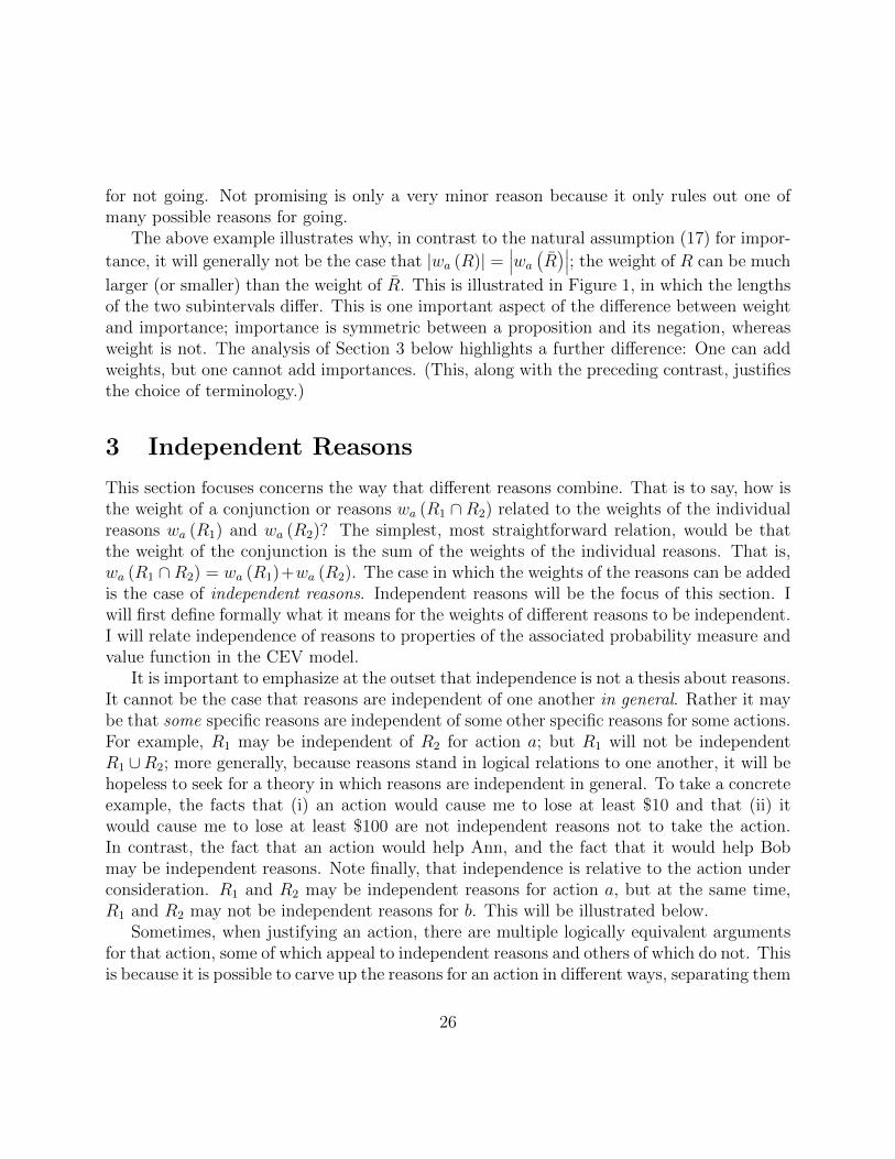
3 Independent Reasons

This section focuses concerns the way that different reasons combine. That is to say, how isthe weight of a conjunction or reasons wa (R1 ∩R2) related to the weights of the individualreasons wa (R1) and wa (R2)? The simplest, most straightforward relation, would be thatthe weight of the conjunction is the sum of the weights of the individual reasons. That is,wa (R1 ∩R2) = wa (R1)+wa (R2). The case in which the weights of the reasons can be addedis the case of independent reasons. Independent reasons will be the focus of this section. Iwill first define formally what it means for the weights of different reasons to be independent.I will relate independence of reasons to properties of the associated probability measure andvalue function in the CEV model.

It is important to emphasize at the outset that independence is not a thesis about reasons.It cannot be the case that reasons are independent of one another in general. Rather it maybe that some specific reasons are independent of some other specific reasons for some actions.For example, R1 may be independent of R2 for action a; but R1 will not be independentR1 ∪R2; more generally, because reasons stand in logical relations to one another, it will behopeless to seek for a theory in which reasons are independent in general. To take a concreteexample, the facts that (i) an action would cause me to lose at least $10 and that (ii) itwould cause me to lose at least $100 are not independent reasons not to take the action.In contrast, the fact that an action would help Ann, and the fact that it would help Bobmay be independent reasons. Note finally, that independence is relative to the action underconsideration. R1 and R2 may be independent reasons for action a, but at the same time,R1 and R2 may not be independent reasons for b. This will be illustrated below.

Sometimes, when justifying an action, there are multiple logically equivalent argumentsfor that action, some of which appeal to independent reasons and others of which do not. Thisis because it is possible to carve up the reasons for an action in different ways, separating them

26

into either independent parts or non-independent parts. An interesting question that arisesis: Are justifications for actions in terms of independent reasons superior to justifications interms of non-independent reasons? This is discussed in Section 3.5.

Before proceeding, some preliminaries are required.

3.1 Preliminaries

Throughout this section (I mean all of Section 3), I fix a weight function w = (wa : a ∈ A),where for each a ∈ A, wa : G+ → R, and an associated pair (V, P ) of a value function andprobability measure. Definition 2 of Section 2.2.3 showed how a weight function w can bederived from a pair (V, P ) via (3). Section 5 below shows how a pair (V, P ) can be derivedfrom a weight function w. So we can think of either w or (V, P ) as primitive and the otheras derived.

3.1.1 Weights of Collections

Say that a collection R = R1, . . . , Rn ⊆ F of reasons is consistent if P [⋂n

i=1Ri] > 0.An event F is consistent with R if R ∪ F is consistent. Say that R is logicallyindependent (LI) if ∀I ⊆ 1, . . . , n, Ri :∈ I ∪ Ri : i ∈ I is consistent, whereI := 1, . . . , n \ I.21

We can extend the notion of the weight of a reason to collections of reasons. In particular,define the weight of a consistent collection of reasons R = R1, . . . , Rn for/against a as:

wa(R) = wa

(n⋂

i=1

Ri

).

In other words, the weight of a collection of reasons is just the weight of their conjunction(or, more formally, their intersection). The hatˆdifferentiates weight applied to a collectionof reasons from weight applied to a single reason.

3.1.2 Conditional Weights

We can also define conditional weights. That is, we can define the weight of a reason condi-tional on having accepted some other reasons. This is the weight of the reason not from theinitial deliberative position in which knowledge of all relevant reasons has been suspended

21Of course, in its details, this definition differs from the standard definition of logical independence.However, logical independence has the right spirit: The idea is that any combination of the propositionscould be true while the others are false. This is a weak form of independence, weaker, than, say, causalindependence or probabilistic independence.

27

(see Sections 2-4), but from an intermediate deliberative position in which some of thesereasons have been accepted again. The weight of reason R0 for/against a conditionalon R (where R = R1, . . . , Rn) is:

wa (R0 |R ) = E[ÁVa ∣∣∣∣∣R0 ∩

(n⋂

i=1

Ri

)]− E

[ÁVa ∣∣∣∣∣ n⋂i=1

Ri

]. (18)

That is to say, wa (R0 |R ) is the difference in the expected value of a that conditioningon R0 makes when one has already conditioned on the reasons in R. For any propositionR1 ∈ G+, I write wa (R0 |R1 ) instead of wa (R0 |R1), so that, in particular, wa (R0 |R ) =wa (R0 |

⋂ni=1Ri ) . Observe that wa (R |∅) = wa (R). Observe also that

wa (R0 |R ) = wa (R0 ∪R)− wa (R) . (19)

If one wants to take weights, rather than values and probabilities, as basic, then then onecan treat (19) as the definition of conditional weight wa (R0 |R ), and treat (18) as a derivedproperty.

3.2 Definition of Independent Reasons

We are now in a position to define the independence of reasons.

Definition 4 R is a collection of independent reasons for/against a if and only if forall R0 ∈ R and all for all nonempty S ⊆ R with R0 6∈ S ,

wa (R0 |S ) = wa(R0).

To abbreviate, we also say that R is a-independent.

In other words, R is a collection of independent reasons if conditioning on any subset ofreasons does not alter the weight of any reason outside the set.

I will find it convenient to work with a stronger notion of independence. Let R =R1, . . . , Rn be a collection of logically independent reasons (see Section 3.1.1). If T ⊆ R,let

RT := R : R ∈ T ∪ R : R ∈ R \T .

That is, RT is the set of reasons that result by “affirming” the reasons in T (treating these astrue) and “disaffirming” the rest (treating these as false). For example, if R = R1, . . . , R5and T = R1, R3, R4, then RT = R1, R2, R3, R4, R5.

28

Definition 5 R is a collection of strongly independent reasons for/against a if andonly if for all T ⊆ R, RT is a-independent. To abbreviate, we say that R is stronglya-independent.

Thus, a collection of reasons is strongly a-independent if, negating any subset to the reasons,the collection remains independent. The reader may observe that for probability measures –as opposed to weight functions – the conditions of independence and strong independence areequivalent. In other words, let R1, . . . , Rn, be independent events according the probabilitymeasure µ, then if we take the complement of any subset of these events arriving at acollection such as R1, R2, R2, . . . , Rn−1, Rn, the resulting collection must also be independentaccording to µ. However, the weight function wa is not a probability measure, or even asigned measure – it is not additive22 – and strong a-independence is indeed a property thatis harder to satisfy than a-independence. Appendix B presents an example illustrating this.

3.3 Weighing Reasons and Maximizing Expected Value

This section establishes a relationship between weighing reasons and maximizing expectedvalue. In the CEV model, these two apparently quite different visions of decision-makinghave the same structure. In the case in which reasons are independent, adding the weightsof reasons coincides with maximizing expected value.

Let us return to the position of deliberative uncertainty. Imagine that, initially, at time0, you know nothing. Then at time 1, you will learn various facts. In particular, recallthat G is the set of potential reasons. Let I ⊆ G . I assume that I , like G , is a σ-field(i.e., closed under complementation and countable intersection). The propositions in I areprecisely those that you will learn, if true, at date 1. That is, for all propositions R in Ithat are true at state ω, (i.e., ω ∈ R) you will learn R at date 1 in ω if and only if R ∈ I .You will never “learn” any false propositions. What you learn depends on the state ω. So Irepresents your information. For simplicity, I assume that I contains only countably manypropositions and each nonempty I ∈ I has nonzero probability: P (I) > 0. Let I (ω) be theconjunction of all propositions that you learn at ω. Formally, I (ω) =

⋂ I ∈ I : ω ∈ I .The above assumptions imply that P (I (ω)) > 0 for all ω ∈ Ω. Observe that I (ω) is itselfa proposition in I .

We imagine that the state is chosen according to the probability measure P . Afterreceiving your information at date 1, you choose an action from the set A0, which includesthe default action d, and all alternative actions. In fact, it is not important that the stateis actually chosen according to P . What matters is only that at state ω, you evaluate theexpected value of actions in the same way that you would if the state had been chosen

22That is, when R1 and R2 are disjoint, it is not generally the case that wa (R1 ∪R2) = wa (R1)+wa (R2).

29

according P to and you updated on your information I (ω). Thus the expected value thatyou assign to action a at state ω is E [Va |I (ω) ] .

Definition 6 A consistent collection R = R1, . . . , Rn ⊆ I of reasons is a-complete iffor all I ∈ I that are consistent with R (i.e., P [I ∩ (

⋂ni=1Ri)] > 0), wa(I|R) = 0.

In other words, a collection of reasons is a-complete if there are no other potential reasons(in I ) that have any weight for a conditional on the reasons in the R.

For each action a ∈ A, define δa = E [Va]. We can call δa the default advantage ofaction a. δa is the value that would be assigned to action a in the absence of any information.If we adopt the position of initial neutrality – before acquiring reasons, there is no basis forpreferring one action over the other, (see Section 2.2.3), then this amounts to the assumptionthat δa = δb for all a, b ∈ A0 (where recall, A0 also contains the default). For (21) below,observe that I adopt the standard convention that

⋂0j=1Rj = Ω.

Proposition 1 Let Ra =¶Ra

1, . . . , Rana

©and Rb =

¶Rb

1, . . . , Rbnb

©be consistent collections

of reasons contained in I , and let R0 := (⋂na

i=1 Rai ) ∩

Ä⋂nbi=1R

bi

ä. Assume initial neutrality.

Assume further that Ra is a-complete and Rb is b-complete. Then,

∀ω ∈ R0, E [Va |I (ω) ] ≥ E [Vb |I (ω) ]⇔ wa (Ra) ≥ wb (Rb) . (20)

Also,

∀ω ∈ R0, E [Va |I (ω) ] ≥ E [Vb |I (ω) ]⇔na∑i=1

wa

ÑRa

i

∣∣∣∣∣∣i−1⋂j=1

Raj

é≥

nb∑i=1

wb

ÑRb

i

∣∣∣∣∣∣i−1⋂j=1

Rbj

é.

(21)

If Ra is a-independent and Rb is b-independent, then,

∀ω ∈ R0, E[Va|I (ω)] ≥ E[Vb|I (ω)]⇔na∑i=1

wa (Rai ) ≥

nb∑i=1

wb

ÄRb

i

ä. (22)

What the result shows is that when you choose by weighing reasons, then, structurally, itis as if you chose by maximizing expected value conditional on the information that youreceived. We imagine that the above described updating occurs in the position of delibera-tive uncertainty. One could also give this scenario the interpretation of actual uncertainty.Then the interpretation would be that if you maximize expected value conditional on your

30

information, then structurally, it is as if you are weighing reasons.23 I view the value of thisresult as resting in the translation manual it provides between the languages of maximizingexpected value and of weighing reasons.

The result suggests the following three step decision procedure: (i) for each action a,identify a set Ra of reasons that is sufficient to make as complete an evaluation of action aas our knowledge will allow, (ii) determine the aggregate weight of the reasons Ra for actiona relative to a default, using the same default for each action, and (iii) choose the action awith the maximum aggregate weight of reasons.

Suppose that in step (i), we determine that some reason R does not belong to Ra. Thisdoes not mean that as a stand-alone reason R has no weight for or against a; it means onlythat we can find a set of reasons Ra that is complete for a and that does not include R.Then we do not need to consider R further in evaluating a. It may be that R does belongto Rb. So we may use different reasons determine the aggregate weight of reasons in favorof or against actions a and b; having used these different reasons, we need only compare thederived aggregate weights to decide between a and b.

For example, in deciding whether to become a doctor or lawyer, I may appeal to the factthat I am squeamish as a reason against becoming a doctor. My squeamishness may or maynot be relevant to my becoming a lawyer, but, in any event, if I find a complete set of reasonsfor evaluating the prospect of becoming a lawyer that does not include my squeamishness,then my squeamishness will contribute to the aggregate weight in favor or against being adoctor and not to that in favor or against being a lawyer.

Suppose that we accept the decision metric of maximizing expected value subject toavailable information. Then, Proposition 1 says that adding the weights of the reasons foreach of the reasons is a legitimate way of making the better decision if the reasons supportingeach action are independent for that action (see (22)). If the reasons supporting an actionare not independent, it is not legitimate to add their weights.

However, a more general procedure is always valid, whether the reasons supporting ac-tions are valid or not. In this procedure, we add not the unconditional weights but conditionalweights. In particular, we perform the following procedure in evaluating action a:

• Start with the unconditional weight wa (Ra1),

• then add the weight wa (Ra2 |Ra

1 ) of R2 conditional on R1,

• then add the weight of wa (Ra3 |Ra

1 ∩Ra2 ) of R3 conditional on R1 and R2,

23I have suggested above that if we use actual, rather than deliberative, probability, then the weights thatwe assign may not correspond to the weights that we might intuitively feel should be assigned. The mainpoint here is that the two different views of decision-making are structurally similar.

31

• . . . ,

• and finally add the weight wa

ÄRa

na|⋂na

i=1Rai

äof Ra

naconditional on all preceding reasons

to arrive at the aggregate weight of all reasons for or against a.

That is, we add the weight of reasons Rai one at a time, each time, conditioning on reason

just added (in addition to the reasons previously conditioned on) before taking the weightof the next reason Ra

i+1. This is the procedure captured by (21) in Proposition 1. Observethat the reasons in Ra can be added in any order, using this procedure, and we will arriveat the same aggregate weight.

One might think that in assessing the weight of a reason Rai for or against action a, we

should consider the marginal contribution of the reason to overall weight conditional onall other reasons

wa (Rai |all other reasons) = wa

ÑRa

i

∣∣∣∣∣∣⋂j 6=i

Raj

é(23)

That is, rather than retreating to a position in which we suspend knowledge of other operativereasons, to determine its weight, we instead consider the effect of taking reason Ra

i intoaccount holding fixed all other reasons that we know to obtain.

Observe that when reasons are not independent, we cannot add the marginal contribu-tions (23) to arrive at total weight wa (R), but when Ra is a-independent, then

wa (Rai ) = wa

ÑRa

i

∣∣∣∣∣∣i−1⋂j=1

Raj

é= wa

ÑRa

i

∣∣∣∣∣∣⋂j 6=i

Raj

é,

so we can arrive at aggregate weight equivalently by adding weights of any of the three formswa (Ra

i ), wa

(Ra

i

∣∣∣⋂i−1j=1R

aj

), or wa

(Ra

i

∣∣∣⋂j 6=iRaj

).

Proposition 1 assumed initial neutrality. How would the proposition have changed if wehad not assumed initial neutrality? (20) would have become

∀ω ∈ R0, E [Va |I (ω) ] ≥ E [Vb |I (ω) ]⇔ wa (Ra)− wb (Rb) ≥ δb − δa.

That is, a has a higher expected value than b if and only if the weight of the reasons fora are in excess of the weight of reasons for b by at least the difference between the defaultadvantage of b over a, δb−δa. The other parts of the proposition would be modified similarly.

32

3.4 Chararacterizations

This section presents some characterizations of (strongly) independent reasons in terms ofthe value function V and probability measure P . Throughout, I hold fixed some set ofpotential reasons R = R1, . . . , Rn. Let FR be the field generated by R. That is, FR isthe closure of R under intersection and complementation. Since FR contains only finitelymany sets, there is no distinction between FR ’s being a field and FR ’s being a σ-field. Arandom variable is a function X : Ω → R that is measurable with respect to F . For anyrandom variable X, define XR = E [X |FR ]. For a formal treatment of measurability andfor what it means to condition a random variable on a σ-field, see Sections 13 and 34 ofBillingsley (1995). For any event R ∈ F , 1R is the indicator function that has value 1 instates ω ∈ R and value 0 in states ω 6∈ R.

I will now state three joint conditions on V, P, and R, which I will call independenceconditions. Within each of these conditions, when I use the term “independence”, I meanprobabilistically independence with reference to the probability measure P .

IC1 There exists random variables Ui, i = 1, . . . , n such that:

1. ÁVa =∑

i Ui, and

2. URi , R1, . . . , Ri−1, Ri+1, . . . , Rn are mutually independent for i = 1, . . . , n.

3. URi , R1, . . . , Ri−1, Ri+1, . . . , Rn are mutually independent conditional on Ri and

conditional on Ri for i = 1, . . . , n.

IC2 1. ÁV Ra =

∑ni=1w (Ri) 1Ri

+∑n

i=1wÄRi

ä1Ri

+ E[Va]

2. R1, . . . , Rn are mutually independent.

IC3 There exists random variables Zji , i = 1, . . . , n, j = 0, 1 such that:

1. ÁVa =∑n

i=1 Z1i 1Ri

+∑n

i=1 Z0i 1Ri

2.ÄZj

i

äR, R1, . . . , Rn are mutually independent for i = 1, . . . , n and j = 0, 1.

The following definition is useful: R contains an a-empty reason if there exists i suchthat for all J ⊆ 1, . . . , n \ i, wa (Ri |

⋂j∈J Rj ) = 0. An a-empty reason is a reason that has

no weight, no matter which other reasons we condition on.

33

Proposition 2 Suppose that R contains no a-empty reasons. Then the following conditionsare equivalent:

1. R is strongly a-independent.

2. V, P, and R jointly satisfy IC1.

3. V, P, and R jointly satisfy IC2.

4. V, P, and R jointly satisfy IC3.

Observe that condition 1, like the other conditions, depends on V and P as well as R. Eachof the independence conditions IC1-IC3 have a similar flavor: (i) The value function canbe represented as a sum of functions, each of which depends on only one of the reasons Ri,and (ii) the different reasons are probabilistically independent. Intuitively, (ii) means thatupdating on one of the reasons does not convey information about any of the other reasons.

3.5 An Example

Suppose that I am a utilitarian. Suppose moreover that I am considering a project thatwould be good for Ann but bad for Bob. My value function might then be the sum of Ann’sutility UA and Bob’s utility UB. Using Proposition 2 and specifically the equivalence ofindependence of reasons and IC1 to justify treating the effect on Ann and the effect on Bobas independent reasons. This example, and in particular the technical details, are discussedin Appendix C.

Here, I just note a few interesting aspects of the example. Suppose that the effects ofthe project can be decomposed into effects on the agent’s wealth and on their health. Theninstead of arguing for or against the project by appeal to reasons concerning the agent’sutilities, we can argue by appeal to reasons concerning the aggregate effects on wealth andthe aggregate effects on wealth. Under certain assumptions, the aggregate effects on wealthwill constitute reasons that are independent of the aggregate effects on health.

This highlights that we may sometimes be able to argue for courses of action in differentways. We can appeal to reasons about utilities or reasons about wealth and health. Eachsets of reason may cut up the world in different ways. At the same time, each set of reasonsmay be redundant in the presence of the other, and yet each individually may be part of anargument for or against the course of action.

It may sometimes happen that two sets of reasons are equivalent in terms of the infor-mation they convey but cut up the world in a different ways. One argument is in terms ofindependent reasons and the other is not. This raises the question of whether the argument

34

in terms of independent reasons is in some sense better and to be preferred. This is discussedfurther in Appendix C.

3.6 Quasi-weights and Neutral Defaults

I have emphasized above that a collection of reasons might be independent for one action awhile not being independent for another action b. Recall however that weights are definedin terms of a second order difference, involving both a variation in action (from a to d) anda variation in whether the reason R is known to hold. This is expressed explicitly in (6). Sofor R to be a-independent involves a relation of R to both Va and Vd. I now briefly considerhow independence might be defined in relation to Va only.

Inert default. Say that the default is inert if Vd (ω) = 0 for all ω ∈ Ω.24 In other words,the default is inert if it is an action that has the same value in every state of the world. Inthis case

wa (R) = E [Va |R ]− E [Va] , (24)

so that the weight of a reason depends only on Va, and indeed we can replace all instancesof ÁVa by Va above. This is the simplest case in which a-independence can be defined solelyin reference to the relation of R to Va. Observe that weight is still defined comparatively –that is, in comparison to the default – as in (5). (24) is a consequence of the inertness of thedefault, not a definition. Accordingly, the objection to noncomparative definition of weightraised in Section 2.2.5 does not apply.25

Quasi-weights. Define the quasi-weight of a reason to be wa (R) = E [Va |R ] − E [Va] .This is not a genuine weight for the reasons set out in Section 2.2.5. For any set R of reasonsand reason R0, define the conditional quasi-weight of R0 given R analogously to the waythat conditional weights were defined in Section 3.1.2 with Va playing the role of ÁVa. Saythat R is quasi-a-independent if for all S ⊆ R, and R0 ∈ R \S , wa (R0 |S ) = wa (R0).This is analogous to Definition 4. One can prove a result analogous to Proposition 2 withquasi-weights rather than weights. So while quasi-weights are not genuine weights for thereasons explained in Section 2.2.5, they may still be a good guide to decision-making. Inparticular, when we have quasi-independent reasons for different actions, we can add thequasi-weights to decide which action is best.

24More generally, we can say that the default is inert if Vd (ω) = r for all ω ∈ Ω for some real number r.25In particular, it is not possible for good news to count as a reason for every action because there is no

event that raises the value of the default. It is perfectly sensible that some event which raises the value ofevery action but the default be a reason to do anything but the default.

35

4 Deliberative Probability

This section interprets the notion of probability in the CEV model. I elaborate the inter-pretation that I call deliberative probability. This interpretation corresponds to the positionof deliberative uncertainty (see Section 2.1).

4.1 Conventional Interpretations of Probability

First, I mention the more conventional interpretation that corresponds to the situation ofactual uncertainty. Probability may be interpreted subjectively as giving the agent’s degreeof belief in various propositions. Probability can also be interpreted as objective probabilityif states have objective probabilities and the agent knows what these probabilities are. I referto these conventional interpretations, both the subjective and the objective interpretation,as prospective because they are most relevant with regard to future events.26

I think that the theory is interesting under this interpretation. If the CEV model isinterpreted in this way, then the model is well suited to the evidential interpretation ofreasons and their weight. This interpretation is valuable because it provides a translationmanual between updating expected value on information, which is well understood, and theweighing of reasons, which is more difficult to grasp. It is valuable to have such a translationmanual between these theories even if one thinks that the translation is not perfect.

These advantages notwithstanding, the conventional interpretation is not my preferredinterpretation of the model. In this section, I will spell out my preferred interpretation interms of deliberative probability.

4.2 Interpreting Deliberative Probability, Part 1

Deliberative attitudes. I start with the basic idea of deliberative attitudes. To motivatethis idea, consider three reasons that may bear on my going to the movies with Jim:

• Rp : I promised Jim that I would go to the movies with him.

• R` : Jim loves going to the movies with a friend.

• Rh : Jim is a human (as opposed to a dog).

26It is of course possible to discuss objective and subjective probability with respect to past events. Forexample, if a fair coin was flipped yesterday, then the objective probability of its coming up heads was 1

2yesterday. We may also recall that our subjective estimate of the chances of rain yesterday was 1

3 .

36

Suppose I know that Rp, R`, and Rh are true. I want to assess the weight of Rp for goingto the movies with Jim. To assess the specific weight of Rp, I may want to abstract awayfrom my knowledge of other reasons. After all, it is the weight of Rp alone that I wouldlike to determine. But what does this “abstracting away” consist in? Specifically, to assessthe weight of Rp, what attitude do I adopt toward R` and Rh? Consider Rh specifically.In assessing the weight of my promise to go to the movies with Jim, can I really adoptno attitude toward the proposition that Jim is a human? No, in considering Rp, I mustform some coherent picture of the situation and so take some attitude toward R` and Rh.The uncertainty in the position of deliberative uncertainty described in Section 2.1 mustincorporate such an attitude.

Deliberative probability I will now develop a picture of what it means to abstract awayfrom other reasons in such a way that a coherent picture of the situation is maintained.Imagine that R0, R1, . . . , Rn is a list of propositions, each of which you know to be true,and each of which is a reason for or against action a as opposed to the default d.27 Imaginefurther that for the purpose of individually assessing the weight of each of these propositionsas reasons, you retreat to a deliberative position in which you suspend your knowledge ofthese propositions (as in Sections 2.1 and 2.2).

In the CEV model, your attitude toward the truth of R0, . . . , Rn in the above deliberativesituation is modeled via a deliberative probability measure P . The probability measure P rep-resents your deliberative attitude. It does not represent your actual beliefs. By assumption,you know that R0, . . . , Rn obtain, but P only assigns these propositions certain probabilities.For the purposes of deliberation, you treat R0 as if you assign R0 probability P (R0). P (R0)is the probability you assign to R0 when you suspend your belief in R0, and also suspend yourbelief in the other reasons R1, . . . , Rn. You do not “take reasons R1, . . . , Rn into account”.By not taking these reasons into account, I do not mean that you ignore the possibility thatthey obtain; I mean that you retreat to a position in which you suspend your belief in them,which is represented as assigning them some probability.

You may also find it useful to contemplateR0, while taking your knowledge thatR1, . . . , Rn

hold into account. If you suspend your belief in R0, while taking R1, . . . , Rn into account,you will assign R0 a deliberative probability of P (R0 |

⋂ni=1 Rn ).

To better understand how we might actually assign and interpret deliberative probabil-ities, let us return to the example from the beginning of this section of promising to go tothe movies with Jim. Consider again the reasons Rp, R`, and Rh introduced above. PerhapsI assume that P (Rh) = 1 because I never seriously consider the possibility that Jim is not

27Not only do you know that each of R0, R1, . . . , Rn is true, but you also know the status of each of thesepropositions as a reason for or against action a.

37

human. Suspending belief about this is not useful for deliberative purposes.I may assume that P (R`|Rp) = P (R`). In other words, R` and Rp are independent from

the standpoint of deliberative probability. This means that taking Rp to be true for thepurpose of deliberation does not cause a change in attitude toward R`. Rp – that I promised– is a stand-alone reason that conveys no information about R` – whether Jim loves going tothe movies with a friend. Setting P (R`|Rp) = P (R`) amounts to taking the attitude that thepromise can be considered as a reason separately from Jim’s attitude toward the experience:As a justification, a promise speaks for itself.

Alternatively, I may have a deliberative probability measure such that P (R`|Rp) > P (R`).This could be interpreted as meaning that the reason Rp I am considering is inherently apromise to a friend who (I believe) wants to go to the movies: In deliberation, promising(Rp) inherently conveys information about my friend’s desire to go (R`). In the next section,I will be a little more precise than I have been above and offer an interpretation for what itmeans for P (R0) > 1

2.

4.3 Interpreting Deliberative Probability, Part 2

This section provides a more thorough interpretation of deliberative probability. The analysisis a bit more formal than that of Section 4.2, and relies on the formal properties of weight.

Let us formally define a weight function to be a collection w = (wa : a ∈ A), wherewa : G+ → R or all a ∈ A. (Recall that A includes all actions other than the default.) Anysuch collection is a weight function. An expectational weight function is a weight functionthat can be derived from that CEV model (see Section 2.2) for some choice of basic valuefunction V and probability measure P via equation (5).

The basic approach I will take here will be to assume that the agent already has a graspof the weight that various reasons have or would have. We can then use these weights toderive implicit probabilities in the deliberative position. Section 5 below shows that ratherthan taking value and probability as primitive and deriving weight, we can take weight asprimitive and derive value and probability. The derived values and probabilities will be suchthat it is as if the weights were derived from values and probabilities.

Proposition 3 Let w be an expectational weight function, suppose that both R and R belongto G+, and let a and b belong to A. Then

1. Probability is Implicit in Weight. Suppose that wa (R) 6= 0. Then

P (R) =wa

ÄRä

wa

ÄRä− wa (R)

=

∣∣∣wa

ÄRä∣∣∣

|wa (R)|+∣∣∣wa

ÄRä∣∣∣ =

wa (R)

ia (R)(25)

38

Consequently,

|wa (R)| >∣∣∣wa

ÄRä∣∣∣ if and only if P (R) <

1

2. (26)

2. Opposite Valences of a Reason and Its Negation. wa (R) > 0 if and only ifwa

ÄRä< 0; wa (R) = 0 if and only if wa

ÄRä

= 0.

3. Constant Weight Ratio of a Reason and Its Negation. If wa

ÄRä6= 0, then

wa(R)

wa(R)= −1−P (R)

P (R); consequently, if wa

ÄRä6= 0, and wb

ÄRä6= 0, then

wa (R)

wa

ÄRä =

wb (R)

wb

ÄRä . (27)

The key fact that generates all of the properties in this proposition is the law of iteratedexpectations. The formula (25), particularly the first equality, is familiar from Bolker-Jeffreydecision theory (Bolker 1967, Jeffrey 1990). Jeffrey expresses probability of a proposition Xas the ratio des X

des X−des X, where des X is the desirability of X.28 Desirability and weight have

the same properties because both are conditional expectations.29

Equation (25) shows how deliberative probabilities can be derived from weights. Theprobability of a proposition is the ratio of its weight to its importance. For convenience, Iagain display Figure 1 here.

• • •EîÁVa |Ró E

îÁVaó E[ÁVa ∣∣∣R]

|wa (R)|∣∣∣wa

ÄRä∣∣∣

|ia (R)|

︸ ︷︷ ︸︸ ︷︷ ︸︷ ︸︸ ︷

Figure 1: Weight and Importance.

It is instructive to focus on (26), which tells us that a proposition has probability less than12

precisely if the weight it has for some decision between an alternative a and the default

28The above expression for probability in terms of desirability applies when des T is normalized to equal0, where T is a tautology. Also when des T = 0, Jeffery remarks that des X and des X have opposite signsexcept when one of these terms is equal to zero, which corresponds to part 2 of Proposition 3.

29There are also differences. Desirability concerns value of propositions whereas weight concerns second or-der differences in value that involve variations in both actions and events as in (6). Substantively, desirabilityand weight are quite different concepts.

39

is less than the weight that its negation would have for that decision.30 Let us get anintuition for why this is so. By the law of iterated expectations E

îÁVaó = EîÁVa |RóP (R) +

E[ÁVa ∣∣∣R] (1− P (R)). In other words, E

îÁVaó is a probability weighted average of EîÁVa |Ró

and E[ÁVa ∣∣∣R], with probability weights P (R) and 1−P (R). Suppose that P (R) < 1

2. Then

the probability weight on E[ÁVa ∣∣∣R] is greater than that on E

îÁVa |Ró. So EîÁVaó is closer to

E[ÁVa ∣∣∣R] than to E

îÁVa |Ró. This is illustrated by Figure 1 above. As R is less likely than

R, learning that R obtains would move the expected value of ÁVa more than learning that Robtains. On this model, a fact R0 that is “taken for granted” in the sense that it has a highprobability P (R0) has less weight relative to its negation than a fact R1 that is informative

in the sense that it initially had a low probability P (R1): That is,∣∣∣∣ wa(R0)

wa(R0)

∣∣∣∣ < ∣∣∣∣ wa(R0)

wa(R0)

∣∣∣∣ .This suggest an alternative way of thinking about deliberative probability. Propositions

that have large weight (relative to their negations) have a small deliberative probability.Intuitively if a proposition R would move our evaluation very much, but its negation wouldnot move our evaluation very much, then that proposition is very informative. Thus, ratherthan focusing on the probability of a proposition, we can focus on how informative it is.This we can do by turning the probability measure “upside down”: Define the specificityof a proposition R ∈ F , S (R) by the relation

S (R) = 1− P (R) . (28)

Observation 2 S : F → R is a specificity measure induced by some probability measure onR if and only if:

∀R0, R1,∈ F , S (R0) + S (R1) = S (R0 ∪R1) + S (R0 ∩R1) , (29)

∀R ∈ F , S (R) ≥ 0, S (Ω) = 0, and S (∅) = 1, (30)

∀ Ri∞i=1 ⊆ F , limn→∞

S

(n⋃

i=1

Ri

)= S

( ∞⋃i=1

Ri

). (31)

Moreover, if S is a specificity measure, then

∀R0, R1 ∈ F , R0 ⊇ R1 ⇒ S (R0) ≤ S (R1) . (32)

Condition (29) is an additivity property and (31) is a continuity property. A probabilitymeasure satisfies all of the properties (29)-(31) except that P (∅) = 0 and P (Ω) = 1 whereasS (∅) = 1 and S (Ω) = 0; that is, the values assigned to ∅ and to Ω are exchanged. Likewise

30Observe that if |wa (R)| <∣∣wa

(R)∣∣ for some a, then for all b, if wb (R) 6= 0, then |wb (R)| <

∣∣wb

(R)∣∣.

40

the monotonicity condition is reversed: more inclusive propositions are more probable, butless inclusive propositions are more specific.

Since probability and specificity are interdefinable, we can take either as primitive. Itmay be more intuitive to think in terms of specificity. It will help to consider some examples.Consider the example of promising you that I would go to the movies from Section 2.2.6.It is intuitive that the proposition that I promised you would be more informative than theproposition that I did not promise you. This accounts for the greater weight that promisinghas as a reason for going than not promising would as a reason for not going.

Let us consider a normative proposition such as the proposition R that it is wrong tokill. The proposition R can serve as a reason and it can have weight, and yet it may bedifficult to grasp what it means to assign such a normative proposition a probability.31 First,observe that if we can assign this reason a weight, then its deliberative probability can beviewed as implicit in its weight via (25). Second, it is intuitive to say that the propositionthat it is wrong to kill, assuming that it is true, is much more informative than would beits negation that it is not wrong to kill. We have seen that informativeness or specificity issufficient to determine deliberative probability. To make this vivid, imagine that you knownothing about morality. Then, to learn that it is wrong to kill would dramatically changeyour worldview; it would be very informative. Perhaps it would also be informative to learnthat it is not wrong to kill, but much less so. Accordingly that it is wrong to kill is a veryweighty consideration when it is relevant, whereas, that it is not wrong to kill, were it true,would not argue for much.

Let us revisit Figure 1. Rather than thinking of the importance ia (R) as the sum ofweights wa (R) and −wa

ÄRä

(see Definition 3), we can think of the weight of R as a share ofthe importance of R: that is, that there exists a number λa (R) between 0 and 1 such that:

wa (R) = λa (R) ia (R) .

We refer to λa (R) as R’s share of the importance. Likewise λaÄRä

= 1−λa (R) is R’s shareof the importance. λa (R) represents the proportion of the movement from R to R whichoccurs in the second half, that is, in the movement from the state of ignorance to knowledgeof R.

31To articulate just one aspect of the difficulty, the proposition that it is wrong to kill does not appearto be a contingent fact that may be true in some states of the world and false in others. In order to assignprobabilities (not equal to zero or one) to begin with, we must however be able to imagine “possible worlds”in which it is true that it is wrong to kill and others in which it is false. Observe that we can ask the questionwhether it is wrong to kill. So it seems that there is the conceptual possibility that it is wrong to kill andthe conceptual possibility that it is not wrong to kill. If the model is to apply to normative propositions,then such conceptual possibilities must be modeled as possible states of the world; for instance, there is aconceptually possible world in it is wrong to kill and others in which it is not.

41

A consequence of the CEV model is that the share λa (R) does not depend on the alter-native a that is opposed to the default. Indeed the share of R is its specificity S (R) = λa (R)for all a ∈ A. This does not mean that the weight of a reason is constant across actions. Theweight of a reason R wa (R) – its sign and magnitude – and its weight relative to another

reason R′, wa(R)wa(R′)

can vary across actions a because the importance of the reason ia (R) canvary across actions, but the weight of a reason for an action relative to the weight that itsnegation would have for that action is constant across actions. (The one exception is in thecase that the reason is irrelevant to the action so that wa (R) = 0.) This is expressed by (27)and is illustrated by Figure 2.

• • •EîÁVa |Ró E

îÁVaó E[ÁVa ∣∣∣R]

|wa (R)|∣∣∣wa

ÄRä∣∣∣

|ia (R)|

︸ ︷︷ ︸︸ ︷︷ ︸︷ ︸︸ ︷

• • •EîÁVb |Ró E

îÁVbó E[ÁVb ∣∣∣R]

|wb (R)|∣∣∣wb

ÄRä∣∣∣

|ib (R)|

︸ ︷︷ ︸︸ ︷︷ ︸︷ ︸︸ ︷

Figure 2: The importance of R varies across actions but the share of R is constant.

More generally than (27), the CEV model actually implies that for any four alternatives

a, b, c, and e,wa,b(R)

wa,b(R)= wc,e(R)

wc,e(R).32

Is it plausible that the share of a reason R is constant across decisions? If we think aboutpropositions such as It is wrong to harm people or Ann lacks basic resources, it is plausiblethat these reasons are much more significant than their negations would be regardless of thedecision under consideration. This lends some intuitive plausibility to the constant sharehypothesis. It is important to note that the constant shares condition holds as we varythe two alternatives a and b, but the background information, or other reasons alreadyconditioned on much be held fixed for the constant shares condition to hold. If A and Bare two distinct sets of reasons, the CEV model does not imply that wa(R|A )

wa(R|A )= wb(R|B )

wb(R|B ).

32A further prediction is that if R0 is more informative than R1, in the sense that R0 ⊆ R1, then R0 will

be weightier relative to its negation than R1 would be: wa(R0)

wa(R0)> wa(R1)

wa(R1). This does not mean that R0 is

weightier than R1: It is not implied that wa (R0) > wa (R1).

42

I conclude this section with an example for which the constant shares condition is prob-lematic. The fact that I promised you I would go is a reason to go, and it is also a reason toapologize if I don’t go. My promise may be more important to the decision of whether I goor don’t go than to the decision of whether I don’t go but apologize or don’t go and don’tapologize; the model does not predict that my promise will be equally important to both.

The theory does predict that if the fact that I promised is a strong reason to go but thefact that I did not promise would have been a very weak reason not to go, then the fact thatI promised would have been a much stronger reason to apologize and not go rather than notapologize and not go than the fact that I did not promise would have been not to apologizeand not go as opposed to apologize and go. This may be so. But note that the fact that Idid not promise is at best a very weak reason not to go. On the other hand the fact thatI did not promise may be quite a significant reason not to apologize not go rather than toapologize and not go. Let a, b, c and d be respectively, go, don’t go, don’t go and apologize,and don’t go and don’t apologize. (Action b may include any assumption about apology

that one wishes.) Then the above considerations suggest that∣∣∣∣ wa,b(R)

wa,b(R)

∣∣∣∣ > ∣∣∣∣ wc,e(R)

wc,e(R)

∣∣∣∣ , contrary

to the theory.Note that in the last paragraph I used the phrase “apologize and not go rather than

not apologize and not go” rather than “apologize if I don’t go” because the latter mightamount to conditioning on additional information, which would nullify the constant sharesassumption.33 This makes our intuitions about the example, a little less clear. Still, I thinkthe example is problematic even given this clarification. The theory will have to addressexamples such as this.

4.4 Integrating Deliberative and Actual Uncertainty

In many decision situations, we know the truth of some propositions that are relevant toour decisions while being uncertain about others. We must therefore weigh the reasonsthat we are aware of while considering possibilities of which we are unaware, but which arerelevant to our decisions. This suggests a combination of deliberative and actual probability.Indeed, model encourages thinking in this way. For example, when Proposition 2 analyzesmaximization of expected value conditional on the reasons that we have, it suggests thatthere may be other relevant facts out there that we do not know about.

Integrating these different types of probability is complicated. One approach would beto interpret the probability measure over the field of facts we know as deliberative proba-bility and the probabilities over uncertain events conditional on the facts we know as actual

33In the paragraph before that, when introducing the example, I used “apologize if I don’t go” because itis more intuitive.

43

probabilities. However, this may be an unstable mixture, especially when one considers thedynamics of updating beliefs. Another approach would be to rigorously separate these twokinds of probability. We imagine that we know all the relevant facts and derive the relevantweights by updating to this situation from the deliberative position. Then we step backand account for our actual ignorance and calculate expected weights based on our actualuncertainty. Future work will have to consider these alternatives more closely.

5 Equivalence of Weight and Value

This section establishes an equivalence between weight and value. It shows that we caneither take weight or value as primitive and derive the other. Thus, the two alternatives thatare open to us are:

1. Weight Derived From Value. We can start with value as primitive, and derive thenotion of weight from value. Starting with value really means starting with value andprobability.

2. Value Derived From Weight. Alternatively, we can start with weight as primitive.If we impose certain axioms on weight, we can then derive both value and probabilityfrom weight.

This section establishes the equivalence. This equivalence means that the CEV model neednot to be bundled with the thesis that value is more fundamental with weight. The CEVmodel rather establishes a structural relation and a translation manual between value andweight, provided that weight satisfies certain axioms. We can then argue on philosophicalgrounds about which notion, if either, should be treated as primitive. Or we may prefer toremain agnostic.

Let us assume for simplicity that F = G , that is, that every proposition in F is apotential reason. I modify the definition a weight function slightly. I call a collectionw = (wa : a ∈ A), where wa : F → R and wa (∅) 6= 0 for all a ∈ A a weight function. Forany action a ∈ A and proposition R in Fa, as above, wa (R) is the weight of R for or againsta. Recall that A includes all actions other than the default. So no weight is assigned to thedefault.34

34There are two slight modifications here in the definition of a weight function, in comparison to thedefinition in Section 4.3. First, the domain of each functon wa is F rather than F+. The reason for thisis that, here I will derive a value function from a probability measure and a weight function. Therefore,I do not want to presume which propositions have probability zero ahead of time. The second differenceis that I have assumed that wa (∅) 6= ∅. Since ∅ corresponds to the inconsistent proposition, we are not

44

In the CEV model, wa (R) = EîÁVa |Ró−E

îÁVaó. To simplify the discussion, let us assume

for the moment that EîÁVaó = 0 for all a ∈ A, although this will not be assumed for the formal

results below. Nothing of technical importance is affected by this simplification. Under thesimplification wa (R) = E

îÁVa |Ró. It is useful at this point to indicate that the expectation

is with respect to probability measure P , and so I write wa (R) = EP

îÁVa |Ró .We would like to impose certain axioms on w such that whenever these axioms are

satisfied there exist V and P such that wa (R) = EP

îÁVa |Ró for all a ∈ A and R ∈ F withP (R) > 0. Let us decompose this into two steps. We want to show that there exist a valuefunction V and a collection of probability measures (Pa : a ∈ A) such that

1. (Conditional Expectation) wa (R) = EPa

îÁVa |Ró for all R ∈ F and a ∈ A, and

2. (Common Probability) Pa = Pb for all a, b ∈ A.

Bolker (1966) axiomatized the conditions under a function φ taking events R as inputs hasthe structure of conditional expectation.35 This answers the question: For what functions φwith events as inputs does there exists a random variable X and probability measure P suchthat φ (R) = EP [X |R ]? Bolker presented two axioms which are sufficient for φ to have thestructure of conditional expectation. One of Bolker’s axioms is called averaging.

Averaging: for all R1, R2 with R1 ∩R2 = ∅,φ (R1) ≤ φ (R2)⇒ φ (R1) ≤ φ (R1 ∪R2) ≤ φ (R2), and

The other is called impartiality.36,37 Bolker was working in a slightly different frameworkthan the one I am working with here.38 His axioms are only necessary but not sufficient

really interested in the weight of ∅. It is however technically convenient to assign this proposition a weight.Any nonzero number will do. Unlike the expression, wa (R) for nonempty R, which represents weight in itsintuitive sense, wa (∅) is not intended to be given any intuitive meaning.

35Formally, Bolker axiomatized functions φ of the form φ (R) = M(R)P (R) , where M is a signed measure and

P is a probability measure. The connection to the structure of conditional expectation is for a random

variable X, and event R with P (R) > 0, EP [X |R ] = M(R)P (R) where M (R) =

∫RXdP . By the Radon-

Nikodym theorem a signed measure M (R) is always of the form∫RXdP when M is absolutely continuous

with respect to P .36The impartiality axiom says that for all R1, R2, and R3 which are pairwise disjoint and are such that

φ (R1) = φ (R2) but φ (R3) 6= φ (R2), if φ (R1 ∪R3) = φ (R2 ∪R3), then for all R4 which are pairwise disjointfrom R1 ∪R2, φ (R1 ∪R4) = φ (R2 ∪R4).

37Variants on the impartiality and averaging that appeal to an ordering on propositions rather than afunction φ on propositions form the basis for Bolker-Jeffrey decision theory.

38In particular, for the result in question, Bolker worked with a complete atom free Boolean algebra,whereas I work with a σ-algebra.

45

in my framework for the expectational structure criterion. These differences are primarilytechnical rather than substantive.

I will develop a different axiomatization for the conditional expectation property and thenimpose an additional assumption that imposes common probability. Let me sketch the mainidea. Define Ma (R) =

∫RÁVadPa. Our aim is that wa will be of the form wa (R) = EP

îÁVa |Ró.Equivalently, wa will be of the form wa (R) = Ma(R)

Pa(R). Observe that Ma is a signed measure

and Pa is a probability measure. As we saw in Section 4.3 – see specifically (25) – probabilityPa can be defined in terms of wa. Since Ma (R) = wa (R)Pa (R), it now also follows that Ma

can be defined in terms of weight. So we can simply impose as our basic axioms that Pa isa probability measure and Ma is a signed measure. This gets us the conditional expectationproperty. To get the common probability property, we then simply assume that Pa = Pb, asthis equality can be spelled out in terms of weight. Equivalently, we assume the constantweight ratio property (27).

The one obstacle to the above approach is that Pa is not defined when wa (R) = 0 =wa

ÄRä. I now develop the approach a little more fully to overcome this issue.

Consider a weight function w = (wa : a ∈ A) . For each a ∈ A, let

Fwa :=

¶R ∈ F : wa (R) 6= wa

ÄRä©, (33)

Fwa is the set on which implicit probabilities are well defined if we attempt to define them

according to (25). For each a ∈ A, define Pwa : Fw

a → R and Mwa : F → R by

Pwa (R) =

wa

ÄRä

wa

ÄRä− wa (R)

∀R ∈ Fwa , (34)

Mwa (R) =

wa(R)wa(R)wa(R)−wa(R)

if R ∈ Fwa ,

0 if R 6∈ Fwa ,

∀R ∈ F . (35)

These equations express how Pa and Ma are derived from w as discussed above. I haveindexed Pa and Ma by the superscript w to indicate that they are derived from w.

I now impose the following conditions:

Continuity: ∀a ∈ A,∀ Ri∞i=1 ⊆ F , wa (⋃n

i=1Ri) = limn→∞wa (⋃n

i=1Ri).

Valence: ∀a ∈ A,∀R ∈ F , wa (R) = wa

ÄRä⇒ wa (R) = 0.

Implicit Probability: ∀a ∈ A,∀R1, R2, R3, R4 ∈ Fwa ,

(R1 ∩R2 = R3 ∩R4 and R1 ∪R2 = R3 ∪R4)

⇒ Pwa (R1) + Pw

a (R2) = Pwa (R3) + Pw

a (R4) .

46

Implicit Measure: ∀a ∈ A,∀R1, R2 ∈ F ,

R1 ∩R2 = ∅ ⇒Mwa (R1) +Mw

a (R2) = Mwa (R1 ∪R2) .

Common Ratios: ∀a, b ∈ A,∀R ∈ F ,Äwa

ÄRä6= 0 and wb

ÄRä6= 0ä⇒

wa (R)

wa

ÄRä =

wb (R)

wb

ÄRä . (36)

Implicit Measure and Continuity imply that Mwa is a signed measure. I believe that Implicit

Probability, Continuity and Implicit Measure jointly imply that Pwa is extendible to a prob-

ability measure on F . I have a proof sketch for this last statement, but have not yet verifiedall details (see Remark 1). Common Ratios is equivalent to the claim that Pw

a (R) = Pwb (R)

for all R ∈ Fwa .

In Section 4.3, an expectational weight function was defined as one that is generated bythe CEV model. In this section, I would like to define an expectational model axiomaticallyrather than in terms of the CEV model. So I reset the meaning of the term “expectational”according to the Definition 7 below.

Definition 7 A weight function w is expectational if it satisfies Continuity, Valence, Im-plicit Measure, Implicit Probability, and Common Ratios.

Proposition 5∗ Let w be a weight function. Then the following conditions are equivalent.

1. w is expectational.

2. There exists a probability measure P on (Ω,F ) and a collection (Va : a ∈ A0) of mea-surable real-valued functions on (Ω,F ) such that:

∀R ∈ F , P (R) > 0⇒ wa (R) = EP [Va − Vd |R ]− EP [Va − Vd]

Suppose that w is expectational and there exists b ∈ A and R ∈ F such that both wb (R) 6= 0and wb

ÄRä6= 0. Then, in 2, P is uniquely determined and for any choice of numbers

(δa : a ∈ A) – these δa’s are default advantages (see Section 3.3) – it is consistent to imposethe condition E [Va − Vd] = δa, ∀a ∈ A, and once this is done, for all a ∈ A, ÁVa = Va − Vdis uniquely determined up to a set of P -measure zero, while Vd can be chosen freely. Thusby setting δa = 0, for all a ∈ A, we may always impose initial neutrality consistently with w.

47

Remark 1 Proposition 5 is marked with a star because I have not yet verified all details ofthe proof. I have a detailed proof sketch and have verified many of the details but not all. Inthe remainder of this section I will write as if the proposition were established.

The proposition spells out the what must be assumed about weight in order that a valuefunction and deliberative probability measure can be derived from weight. We saw in Section4.3 how probability P could be derived from weight, namely via (25). How can value bederived from weight? Comparative value can be derived from the Radon-Nikodym derivativeof wa (R)P (R) with respect to P (R). For any δ, there is an (essentially) unique solution ÁVato: ÁVa + δa =

dMwa

dP

EîÁVaó = δa

To understand this, observe that when we don’t assume that EîÁVaó 6= 0, then in general

we have Mwa (R) = wa (R)P (R) =

∫RÁVadP + E

îÁVaóP (R). If we assume initial neutrality,then comparative value is completely determined by weight. In general, if we have thevector δ = (δa : a ∈ A) of default advantages and and an expectational weight function,then comparative value ÁVa = Va − Vd is completely determined. However Va and Vd are notdetermined separately.

It is important to separate two claims: (i) Value and deliberative probability can bederived from weight. (ii) The axioms on weight under which this is so are correspond tointuitive properties of weight. Proposition 5 spells out the details of (i). In the absence ofProposition 5, it would still be clear that there is some class of weight functions such that ifweight is in that class, value and probability are implicitly determined. Proposition 5 spellsout axiomatically what that class is. Proposition 5 does not perform as well on (ii). In par-ticular, it is not intuitively clear that weight should satisfy Implicit Probability and ImplicitMeasure; at least, I do not have a direct argument for this at this time. An alternativewould be to substitute for Implicit Probability and Implicit Weight, Bolker’s Averaging andImpartiality Axioms applied to weight. For example, applied to weight, the averaging axiomsays that if R1 ∩R2 = ∅, if wa (R1) ≤ wa (R2), then wa (R1) ≤ wa (R1 ∪R2) ≤ wa (R2). Thisis a plausible property of weight, as is impartiality (see footnote 36). To take this approachwould require strengthening other technical assumptions. For example, we have not assumedthat F is atom free; for example, F is allowed to be finite in the above result. Note that,given the appropriate technical modifications, in addition to Averaging and Impartiality,Common Ratios would have to be assumed. Finally observe that an indirect argument forImplicit Probability and Implicit Measure is that under the appropriate technical modifica-tions, Averaging and Impartiality would imply Implicit Probability and Implicit Measure.

48

Finally, I mention that in the same way that Bolker-Jeffrey decision theory derives desirabil-ity and probability functions from a preference ordering on propositions, it may be possibleto derive weights, values and deliberative probabilities from a family of strength orderingson reasons.39

6 Conclusion

This paper has presented a formal model of reasons. I have linked comparative value to theweight of reasons. The weight of a reason is analyzed in terms of the way that consideringthe reason alters the comparison between an action and a default. The theory allows one tostudy how reasons interact and characterizes independent reasons. The theory allows one totake either value or weight as primitive and derive the other.

Much remains to be done. One task is to use the model further analyze the two types ofconflict among reasons described in the introduction. Another is to apply the theory to theaggregation of reasons of different individuals, or to help us understand what we should doif aggregation is not appropriate.

A Proofs

The proofs will be inserted in a future draft.

B Independence Versus Strong Independence

In this appendix, I present an example that shows that strong a-independence does not implyindependence. Consider the following tables:ÁVa R2 ∼ R2

R1 0 −1∼ R1 1 0

P R2 ∼ R2

R1 1/3 1/6∼ R1 1/6 1/3

In both tables, I have used the notation ∼ R instead of R for the complement of R to enhancereadability. The table on the left gives the value of a ÁVa as a function of the state ω. I assumethat ÁVa depends only on whether each of the events R1 and R2 obtain or fail to obtain. The

39This strength ordering would have to compare the strength of reason R1 for action a to the strength ofR2 for b.

49

table on the right gives the joint probability of R1 and R2 and their complements. Usingthese tables, we calculate the following (conditional) expectations:

EîÁVaó = 0,

EîÁVa |R1

ó= − 1

3,

EîÁVa |R2

ó=

1

3,

EîÁVa |R1 ∩R2

ó= 0,

E[ÁVa ∣∣∣R1

]=

1

3,

E[ÁVa ∣∣∣R1 ∩R2

]= 1.

So

wa (R1) = EîÁVa |R1

ó− E

îÁVaó = −1

3= E

îÁVa |R1 ∩R2

ó− E

îÁVa |R2

ó= wa (R1 |R2 ) ,

wa (R2) = EîÁVa |R2

ó− E

îÁVaó =1

3= E

îÁVa |R1 ∩R2

ó− E

îÁVa |R1

ó= wa (R2 |R1 ) .

So R1, R2 is a-independent. On the other hand,

wa

(R2

∣∣∣R1

)= E

[ÁVa ∣∣∣R1 ∩R2

]− E

[ÁVa ∣∣∣R1

]=

2

36= 1

3= wa (R2) .

So R1, R2 is not strongly a-independent. It follows that a-independence does not implystrong a-independence.

C An Example: Utilitarianism

This section presents the example briefly discussed in Section 3.5. Specifically, this sectionexamines the weight of reasons from the standpoint of a utilitarian.

There are two agents, Ann and Bob. Given any action a, value given that a is taken isrepresented as:

Va = UAa + UB

a . (37)

UAa and UB

a are utilities of Ann and Bob that depend on the state of the world conditionalon action a being taken. Formally, UA

a and UAb are random variables. That value is given by

the sum of utilities reflects the utilitarian values mentioned above.

50

Suppose that you are considering a project a that will help Ann and harm Bob. Let RA

be the proposition that the the project would help Ann. Let RB be the proposition that theproject would harm Bob.

Assume that the default d is a status quo that involves doing nothing. Specifically UAd ≡ 0

and UBd ≡ 0, or, in words, the default leads to a utility of 0 in every state of the world.

Suppose that for the purpose of deliberation you treat RA and RB as being independentof one another (i.e., in deliberating about the project, when we consider the force of the factthat it will help Ann, we do not take into account the effect on Bob). Formally:

1. UBa and RA are mutually independent both unconditionally and conditional on RB and

on RB.

2. UAa and RB are mutually independent both unconditionally and conditional on RA and

on RA.

Then Proposition 2 implies that RA and RB are independent reasons for/against the project.Now suppose that the project has two sorts of impacts: RW means that the project

would have a positive impact on agents’ wealth. RH means that the project would have anegative impact on agents’ health. For Ann, the wealth effect outweighs the health effect,which is why it helps her. For Bob, the health effect outweighs the wealth effect, which iswhy it harms him. Specifically, the relation between, wealth, health and utility is expressedas follows

UAa = uA(WA

a , HAa ) and UB

a = uB(WBa , H

Ba ).

Here WAa and HA

a are real valued random variables that encode Ann’s level of wealth andhealth at each state of the world, and uA is a utility function that maps Ann’s wealth andhealth to her utility level. I assume that these two variables, wealth and health, determinedAnn’s utility. WB

a , HBa , and uB are defined similarly, but pertain to Bob rather than Ann.

Say that utility is separable in wealth and health if there exist subutility functionsuAw, u

Ah , u

Bw and uBh such that

uA(WAa , H

Aa ) = uAw(WA

a ) + uAh (HAa ),

uB(WBa , H

Ba ) = uBw(WB

a ) + uBh (HBa ).

uAw and uAh are, respectively, Ann’s utility of wealth and utility of health functions, and uBwand uBh are defined similarly for Bob. Then,

Va = uw(Wa) + uh(Ha)

51

where, Wa = (WAa ,W

Ba ) and Ha = (HA

a , HBa ), uw(Wa) = uAw(WA

a ) + uBw(WBa ) uh(Ha) =

uAh (HAa ) + uBh (HB

a ). In other words, rather than expressing the value of action a as the sumof Ann and Bob’s utilities as in (37), we can rewrite utility as the sum of aggregate wealthutility and aggregate health utility.

Let RW be the proposition that the project would have a positive impact on agents’wealth and RH the proposition that the project would have a negative impact on agents’health. If

1. utility is separable in wealth and health,

2. (i) uw(Wa) and RH are independent both unconditionally and conditional on RW

and on RW , and

(ii) uh(Ha) and RW are independent both unconditionally and conditional on RH andon RH ,

Proposition 2 implies that RW and RH are independent reasons. If either condition 1 or2 fails, then RW and RH will generally not be independent reasons. 2 might fail becausehealth and wealth may be causally interrelated and we may want to take this into accountin deliberation.

An action (e.g., our project) may have multiple rationales. There may be multiple waysof cutting up the world. Some (e.g., RA and RB) may be independent – especially if they arein terms of events that concern fundamental ethical categories – in this case the utilitariantakes Ann and Bob’s utilities to be fundamental ethical values out of which overall value isbuilt. Others (e.g., RW and RH) may or may not be independent.

An interesting question that arises here is: Should we prefer independent reasons (RA

and RB) to non-independent reasons (RW and RH) when both are available?Note that in some cases, the competing rationales may each be complete (each is re-

dundant given the other) and they may or may not be equally informative (they may cutthe world into finer or courser slices). I illustrate this through a slight modification of theexample.

I modify the example slightly. RA remains the proposition that the project would helpAnn, but RB now becomes the proposition that the project would help Bob. Let RS be theproposition that the project has the same effect on both: that is, either the project helpsboth Ann and Bob or the project harms both Ann or Bob. Suppose that if the project helpsan agent that leads to an additional utility of 1 relative to the default, and when it harmsan agent, that leads to a loss of a utility of 1, relative to the default. We can represent thepossibilities in two equivalent ways in two different tables.

52

Va RB ∼ RB

RA 2 0∼ RA 0 −2

Va RS ∼ RS

RA 2 0∼ RA −2 0

Figure 5: Two Ways of Cutting Up The Possibilities

Here, I use the notation ∼ R instead of R. Assume that each of the four possibilities ineach of the tables is equiprobable. Observe that the sets of reasons R0 = RA, RB andR1 = RA, RS are logically equivalent not only in that RA∩RB = RA∩RS but in that theygenerate the same field (i.e, set of events constructible via intersection and complementation),so they are in a sense equally informative. Yet only R0 is independent:

wa(RA|RB) = 2−ñ

1

22 +

1

20

ô= 1 =

ñ1

22 +

1

20

ô− 0 = wa(RA)

wa(RA|RS) = 2− 0 = 2 > 1 =

ñ1

22 +

1

20

ô− 0 = w(RA)

While the arguments in terms of the reasons R0 and R1 are in logically equivalent, thereis a case to be made that the argument in terms of R0 is more basic, as reflected by theindependence of the reasons to which it appeals.

References

Alvarez, M. (2016), ‘Reasons for action: justification, motiva-tion, explanation’, The Stanford Encyclopedia of Philosophy .http://plato.stanford.edu/archives/sum2016/entries/reasons-just-vs-expl/.

Arrow, K. (1951), ‘Social choice and individual values’.

Billingsley, P. (1995), Probability and measure, John Wiley & Sons.

Bolker, E. D. (1966), ‘Functions resembling quotients of measures’, Transactions of theAmerican Mathematical Society 124(2), 292–312.

Bolker, E. D. (1967), ‘A simultaneous axiomatization of utility and subjective probability’,Philosophy of Science pp. 333–340.

Broome, J. (1991), Weighing goods, Blackwell Publishers.

53

Broome, J. (2013), Rationality through reasoning, John Wiley & Sons.

Chang, R. (2016), Comparativism: The grounds of rational choice, in E. Lord andB. Maguire, eds, ‘Weighing Reasons’, Oxford University Press.

Dasgupta, P. (2001), Human well-being and the natural environment, Oxford UniversityPress.

Dietrich, F. and List, C. (2007), ‘Arrow’s theorem in judgment aggregation’, Social Choiceand Welfare 29(1), 19–33.

Dietrich, F. and List, C. (2013), ‘A reason-based theory of rational choice’, Nous 47(1), 104–134.

Dietrich, F. and List, C. (2016), ‘Reason-based choice and context-dependence: An explana-tory framework’, Economics and Philosophy 32(02), 175–229.

Jeffrey, R. C. (1990), The logic of decision, University of Chicago Press.

Kearns, S. and Star, D. (2009), ‘Reasons as evidence’, Oxford studies in metaethics 4, 215–42.

List, C. and Pettit, P. (2002), ‘Aggregating sets of judgments: An impossibility result’,Economics and Philosophy 18(01), 89–110.

List, C. and Polak, B. (2010), ‘Introduction to judgment aggregation’, Journal of economictheory 145(2), 441–466.

Lord, E. and Maguire, B., eds (2016), Weighing Reasons, Oxford University Press.

Mongin, P. (1997), ‘Spurious unanimity and the pareto principle’. Working Paper, TheorieEconomique, Modelisation et Applications, Universite de Cergy-Pontoise and CentreNational de Recherche Scientifique.

Raz, J. (1999), Practical reason and norms, Oxford University Press.

Scanlon, T. (1998), What we owe to each other, Harvard University Press.

54