Comparative Visualization Using Cross-Mesh Field Evaluations and

Comparative Visualization Using Cross-MeshField Evaluations and Derived Quantities

Hank Childs1, Sean Ahern2, Jeremy Meredith2, Mark Miller3, and Kenneth I.Joy4

1 Lawrence Berkeley National LaboratoryBerkeley, California, [email protected]

2 Oak Ridge National LaboratoryOak Ridge, Tennessee, [email protected]

3 Lawrence Livermore National LaboratoryLivermore, California, [email protected]

4 Institute for Data Analysis and VisualizationComputer Science DepartmentUniversity of CaliforniaDavis, California, [email protected]

AbstractWe present a data-level comparative visualization system that utilizes two key pieces of technology: (1)cross-mesh field evaluation – algorithms to evaluate a field from one mesh onto another – and (2) a highlyflexible system for creating new derived quantities. In contrast to previous comparative visualizationefforts, which focused on “A−B" comparisons, our system is able to compare many related simulationsin a single analysis. Types of possible novel comparisons include comparisons of ensembles of datagenerated through parameter studies, or comparisons of time-varying data. All portions of the systemhave been parallelized and our results are applicable to tera-scale and even peta-scale data sets.

1 Introduction

One of the most common activities of an analyst is to perform comparisons. These comparisons takedifferent forms: comparing a simulation to experimental data, comparing a simulation to a legacysimulation result, comparing the results of a simulation before and after key algorithmic changes,comparing the results of two simulations with different initial geometries. These are generally “A-B"type comparisons, where two results are compared. Sometimes, however, the comparisons need totake place between a series of data sets, for example when doing a parameter study or looking attime-varying data.

In this paper, we present a powerful system for facilitating data-level comparisons. Our systemincorporates multiple inputs and creates an output data set that reflects a comparison. The systemcombines two key technologies:1. cross-mesh field evaluation (CMFE), where a field from a “donor” mesh is evaluated onto a

“target” mesh, and2. derived quantity generation, where new fields are created from existing onesThese two capabilities combine to form a powerful and flexible system where end users are givengreat latitude to create data sets tailored to application specific comparative metrics.

Given a set of donor meshes M1,M2, ...,Mk each containing a corresponding field F1,F2, ...,Fk,and a target mesh MC, We evaluate each field Fi onto MC, creating a new field on the target mesh.

Dagstuhl PublishingSchloss Dagstuhl – Leibniz-Zentrum für Informatik, Germany

2 Comparative Visualization

These new fields are analyzed using the derived quantity subsystem, creating a new field over MC thatcan be displayed using conventional visualization methods. Cross-mesh field evaluation is related toderived quantity generation because, from the perspective of the target mesh, it results in the creationof a new field. We exploit this relationship by integrating cross-mesh field evaluation with derivedfunction generation in a data-parallel distributed memory implementation, making it applicable to anumber of very large scale problems.

Research related to this effort is addressed in Section 2. Section 3 describes data-level compar-ison methods and illustrates the problems of cross-mesh field evaluation. Section 4 describes oursystem and the data-parallel implementation of cross-mesh field evaluation. Results of this effort aregiven in Section 5, and in the supplementary material.

2 Related Work

Three basic areas of comparative visualization: image-based, data-level, and topological compar-isons have been discussed in the literature (see Shen et al. [1]). Image-based methods generate mul-tiple images, and provide methods by which a user can compare the image data; data-level methodscompare the actual data between input data sets, and provide methods by which the differences canbe compared; and topological-based methods compare results of features generated for each of theinput data sets.

Most image-based comparison systems [2, 3, 4] perform image differencing algorithms on im-ages from multiple inputs. These systems are limited to comparing visualizations where the dataset can be represented by a single image. These techniques are extremely important in the contextof comparison to experimental results, such as in the case with [2] and [4]. The VisTrails systemof Bavoil et al. [5] coined the phrase multiple-view comparative system to describe image-basedsystems where plots are placed side-by-side or potentially overlaid. In multiple-view comparativesystems, the burden is placed on the human viewer to visually correlate features and detect differ-ences.

Topological methods [6, 7, 8] compare features of data sets. Typically, they survey the dataset, create summaries of the data, and develop image-based or data-level methods to visualize thesesummaries.

The ALICE Differencing Engine of Freitag and Urness [9] is a data-level comparison tool. It islimited to comparing data sets that have identical underlying meshes and only allows data differenc-ing comparisons. Shen et al. [1, 10] place data sets on an target mesh and utilize derived quantities toform comparisons. Sommer and Ertl [11] also base their comparisons on data-level methods. Theirsystem employs only connectivity-based differencing, although they also consider the problem ofcomparisons across parameter studies.

Many visualization systems [12, 13, 14] provide subsystems for generating derived quantities.Moran and Henze give an excellent overview in [15] of their DDV system, using a demand drivencalculation of derived quantities. McCormick et al. furthered this approach with Scout [16] bypushing derived quantity generation onto the GPU. Joy et al. [17] have developed statistics-basedderived quantities that greatly expand the uses of derived functions.

Our comparative visualization system has been deployed within VisIt [18], an open source vi-sualization system designed to support extremely large scale data sets. As with many visualizationtools [14, 12], it has a data flow network design that leverages pieces of VTK [19]. A key differ-entiating aspect is its strong contract basis [20], which enables many algorithms to be implementedin parallel. As with the system of Shen et al. [1, 10], the data sets to be compared are placed on atarget mesh and derived quantities are generated. Our system contains the following extensions:

Hank Childs, Sean Ahern, Jeremy Meredith, Mark Miller, and Kenneth I. Joy 3

comparison of more than two input data sets, which enables powerful applications for time-varying data and parameter studies,the flexibility of applying either position-based or connectivity-based comparisons, anda fully parallel, distributed memory solution.

3 Data-level Comparison Methods

Let M1,M2, ...,Mk denote a set of donor meshes, each containing a corresponding field F1,F2, ...,Fk,and let MC denote some target mesh. The cross-mesh evaluation step evaluates each field Fi, fori = 1, ...,k, onto MC, creating new fields FC,i, i = 1, ...,k that represent each of the original fields onthe target mesh. We then employ a function, D(FC,1,FC,2, ...,FC,k)→ ℜ, that takes elements of thek fields as input and produces a new derived quantity. The resulting field FD, defined over MC, isthen visualized with conventional algorithms. (Most previous systems consider only M1 and M2 andvisualize FD = FC,1 - FC,2.)

Mi and Fi can come from simulation or experimental observation. Some common examples are:two or more related simulations at the same time slice, multiple time slices from one simulation, ora data set to be compared with an analytic function.

The target mesh MC can be a new mesh or one of the donor meshes Mi. In practice, we frequentlyuse the latter option. However, this system supports the generation of new arbitrary rectilinear gridswith a user-specified region and resolution.

There are two choices for generating FC,i: the evaluation can be made either in a position-basedfashion or in a connectivity-based fashion. Position-based evaluation is the most common method.Here, the donor and target meshes are overlaid and overlapping elements (cells) from the meshes areidentified. Interpolation methods are applied to evaluate Fi on MC. This technique is difficult to im-plement, especially in a parallel, distributed memory setting, because MC and Mi may be partitionedover processors differently – which requires a re-partitioning to align the data. This re-partitioningmust be carefully constructed to ensure that no processor exceeds primary memory.

Connectivity-based evaluation requires that both the donor mesh, Mi, and the target mesh, MC,are homeomorphic. That is, they have the same number of elements and nodes, and the element-to-node connectivities for all elements are the same. This is often the case if MC is selected fromone of the Mi, because for comparisons across time and/or parameter studies the remaining Mj: j �=itypically have the same underlying mesh. In this case, the value of an element or node in Mi isdirectly transferred to the corresponding element or node in MC. Connectivity-based cross-meshfield evaluation is substantially faster; the difficult task of finding the overlap between elements iseliminated.

For Eulerian simulations (where node positions are constant, but materials are allowed to movethrough the mesh), connectivity-based evaluation yields the same results as position-based evalu-ation but with higher performance. For Lagrangian simulations (where materials are fixed to ele-ments, but the nodes are allowed to move spatially), position-based evaluations are used most often,because connectivity-based evaluations typically do not make sense in the context of moving nodes.However, connectivity-based evaluation allows for new types of comparisons, because comparisonscan take place along material boundaries, even if they are at different spatial positions. Further,connectivity-based evaluations allow for simulation code developers to pose questions such as: howmuch compression has an element undergone? (This is the volume of an element at the initial timedivided its volume at current time.)

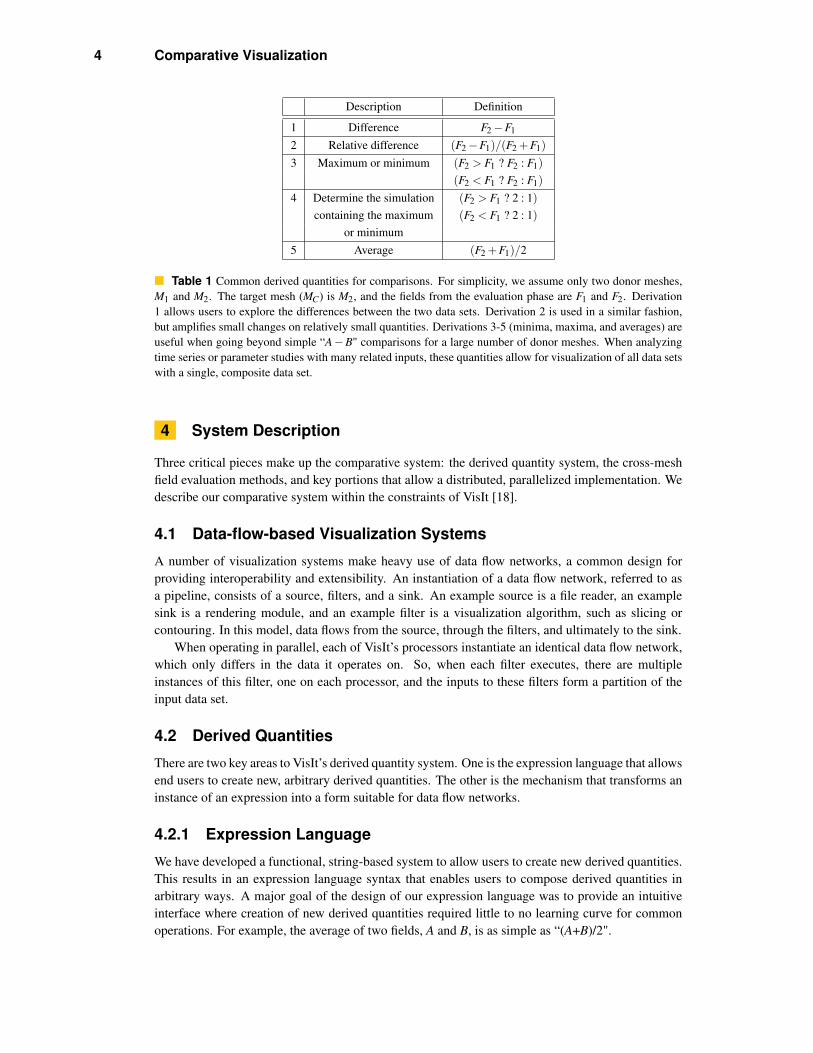
There are limitless forms of derived quantities, FD, that are necessary for different types ofcomparisons in different situations. We list a few of the most frequently used in Table 1 as examples.


Description Definition

1 Difference F2−F1

2 Relative difference (F2−F1)/(F2 +F1)3 Maximum or minimum (F2 > F1 ? F2 : F1)

(F2 < F1 ? F2 : F1)4 Determine the simulation (F2 > F1 ? 2 : 1)

containing the maximum (F2 < F1 ? 2 : 1)or minimum

5 Average (F2 +F1)/2

Table 1 Common derived quantities for comparisons. For simplicity, we assume only two donor meshes,M1 and M2. The target mesh (MC) is M2, and the fields from the evaluation phase are F1 and F2. Derivation1 allows users to explore the differences between the two data sets. Derivation 2 is used in a similar fashion,but amplifies small changes on relatively small quantities. Derivations 3-5 (minima, maxima, and averages) areuseful when going beyond simple “A−B" comparisons for a large number of donor meshes. When analyzingtime series or parameter studies with many related inputs, these quantities allow for visualization of all data setswith a single, composite data set.

4 System Description

Three critical pieces make up the comparative system: the derived quantity system, the cross-meshfield evaluation methods, and key portions that allow a distributed, parallelized implementation. Wedescribe our comparative system within the constraints of VisIt [18].

4.1 Data-flow-based Visualization SystemsA number of visualization systems make heavy use of data flow networks, a common design forproviding interoperability and extensibility. An instantiation of a data flow network, referred to asa pipeline, consists of a source, filters, and a sink. An example source is a file reader, an examplesink is a rendering module, and an example filter is a visualization algorithm, such as slicing orcontouring. In this model, data flows from the source, through the filters, and ultimately to the sink.

When operating in parallel, each of VisIt’s processors instantiate an identical data flow network,which only differs in the data it operates on. So, when each filter executes, there are multipleinstances of this filter, one on each processor, and the inputs to these filters form a partition of theinput data set.

4.2 Derived QuantitiesThere are two key areas to VisIt’s derived quantity system. One is the expression language that allowsend users to create new, arbitrary derived quantities. The other is the mechanism that transforms aninstance of an expression into a form suitable for data flow networks.

4.2.1 Expression LanguageWe have developed a functional, string-based system to allow users to create new derived quantities.This results in an expression language syntax that enables users to compose derived quantities inarbitrary ways. A major goal of the design of our expression language was to provide an intuitiveinterface where creation of new derived quantities required little to no learning curve for commonoperations. For example, the average of two fields, A and B, is as simple as “(A+B)/2".


Of course, users will want to create derived quantities that are more than simple mathematicalconstructs. Support exists in the language for composing scalar quantities into vectors or tensors,and for extracting scalar components back out. Notation for strings, lists, ranges, and strides allowsselection of materials, parts, and other subsets of elements. For accessing other files, either withinthe same sequence or in different sequences, the language supports references by cycle, absolute andrelative time index, and filename. Other named operations are referenced as functions, and a smallselection of the over one hundred available are listed in table 2.

Table 2 Our expression language allows for all of these functions to be combined in arbitrary ways.

Math +, -, *, /, power, log, log10, absval, ...Vector cross, dot, magnitudeTensor determinant, eigenvector, effective (e.g. strain), ...Mesh coordinates, polar, volume, area, element_id, ...

Field Operator gradient, divergence, curl, LaplacianRelational if-then-else, and, or, not, <,≤,>,≥,=, �=

Mesh Quality shear, skew, jacobian, oddy, largest angle, ...Trigonometric sine, cosine,..., arctangent, degree2radian, ...Image Filters mean, median, conservative smoothingMiscellaneous recenter, surf. normal, material vol. fraction, ...

The strength of our expression language lies in the richness of functionality and the interop-erability between these expressions. Consider, for example, computing divergence (�). If a two-dimensional vector F is defined as Px + Qy, then �F = ∂P

∂x + ∂Q∂y . A user can calculate divergence

directly using the built-in function, divergence(). But, for illustrative purposes, it is also straight-forward to calculate divergence using other functions as building blocks: “divF = gradient(P)[0] +gradient(Q)[1]". VisIt has a custom scanner and parser that constructs a parse tree based on expres-sions like this one. Figure 1 contains the parse tree for this divergence expression.

Figure 1 Creation of a derived quantity. On the left, we see an expression’s parse tree. On the right, we seethe linearized data flow network for that parse tree.

When VisIt assembles a data flow network, it relies on an Expression Evaluator Filter (EEF) toconstruct derived quantities. The EEF is typically inserted as the first filter in the pipeline, immedi-ately following the file reader module. In a preparatory phase, the other filters place the names of


their required variables into a list. When executing, the EEF cross-references this list with knownexpression names to determine what derived quantities need to be calculated.

The EEF dynamically creates a sub-network to create needed derived quantities. To do this, itfirst consults the parse trees of the expressions. For each node in each parse tree, a filter that canperform the corresponding operation is placed into the sub-network. Ultimately, this sub-networkreflects a linearized form of the parse trees. The linearization process requires the EEF to do de-pendency checking between all of the parse trees for all of the expressions involved to ensure thatevery filter has the inputs it needs. VisIt’s implementation supports the linearization of any parsetree, including this dependency checking.

Our system supports the accumulation of partial results onto the target mesh MC so that individualFC,i’s can be quickly discarded. While the sub-network is executing, the EEF is able to determinewhen intermediate variables are no longer needed and remove them. Through this mechanism, theEEF is able to successfully handle many related data sets that would otherwise exceed the availablememory.

To perform a cross-mesh field evaluation, the user defines an expression involving built-in func-tions for the evaluation algorithms – position-based or connectivity-based. Like all other expres-sions, the comparison expressions have corresponding filters that can be placed in the sub-networkto perform the cross-mesh evaluation. By combining these algorithms with expressions, users candirect the creation of new, derived quantities from a multitude of sources on the same target mesh.Furthermore, they can manipulate these quantities using all of the previously mentioned expressionsto create interesting comparisons.

Finally, although derived quantity generation typically takes place immediately after reading thedata, it is also possible to defer their evaluation until later in the pipeline. This ability allows for thetarget mesh to be transformed before the cross-mesh field evaluation takes place. This is importantwhen registration is needed, for example for comparison with experimental data.

4.3 Cross-Mesh Field Evaluation

The implementations of the various filters for cross-mesh field evaluation (CMFE) are similar. Theyall have one input for the target mesh and they all are capable of dynamically instantiating an addi-tional data flow network to obtain Mi and Fi. The differentiating point between the CMFE filters ishow they evaluate the fields.

The connectivity-based CMFE algorithm is straightforward. For each element or node, it placesFi onto MC to create FC,i. The only subtlety is guaranteeing that the partitioning of the input data (ina parallel setting) is done so that each processor operates on the same chunks of data.

The position-based CMFE algorithm is complex. There are three major challenges:1. the overlay step – identifying which elements of the donor mesh Mi overlap with an element in

the target mesh MC.2. the interpolation step – fitting an interpolant for the field on the target mesh MC such that it

matches, as closely as possible, at key points on the donor mesh Mi.3. Managing the distribution of data to maximize parallel computational efficiency in a distributed-

memory environment.

4.3.1 The Overlay Step

We use interval trees [21] to efficiently identify elements from meshes Mi and MC that overlapspatially. We start by placing all elements from Mi into the interval tree. Then, for each elementof MC, we use its bounding box to index the interval tree and find the list of elements from Miwith overlapping bounding boxes. We examine this list to find the elements that truly overlap (as


opposed to only having overlapping bounding boxes). If MC contains NC elements and Mi containsNi elements, then the time to generate the tree is O(Nilog(Ni)) and the time to locate the elements ofMi that overlap with an element of MC is O(log(Ni) + α), where α is the number of elements fromMi returned by the search. This gives a total time of O((NC + Ni)*log(Ni)). Note that α is amortizedout for all but degenerate mesh configurations.

4.3.2 Field Interpolation

For each position x on the target mesh MC, we evaluate the field on the donor mesh Mi at x, andassign the value at that location to MC. This method was chosen because it favors performance overaccuracy. A good improvement to our implementation, however, would be to add the use of weightedaveraging with weights based on volume overlaps.

4.3.3 Parallel Implementation

The final piece of the problem is to perform cross-mesh field evaluations in a parallel, distributed-memory environment. The key issue deals with spatial overlap. When a processor is evaluating afield from mesh Mi onto the target mesh MC, it must have access to the portion of Mi that overlapsspatially with the portion of MC it is operating on. Our strategy for this issue is to create a spatialpartition to guide re-distribution of both meshes for the evaluation phase. Unfortunately, the spa-tial partition must be created with great care. If the partition divides space into regions that coverappreciably different numbers of elements, it will lead to load imbalances and potentially exhaustmemory. Therefore, we focus on creating a balanced spatial partitioning, where “balanced" impliesthat every region contains approximately the same number of elements, Et (see Figure 2). The Et el-ements from each region may contain different proportions of elements from MC and Mi; in general,it is not possible to have this proportion be fixed and Et be equal on all processors.

Figure 2 In the upper left, two meshes, Mi and MC, are shown. Assume the red portions are on processor1, blue on 2, and so on. We employ an iterative strategy that creates a balanced spatial partition. We start bydividing in X, then in Y, and continue until every region contains approximately 1/Nth of the data, where N is thetotal number of processors. Each processor is then assigned one region from the partition and we communicatethe data so that every processor contains all data for its region. The data for processor 3 is shown in the last setof figures.

The algorithm to efficiently determine a balanced spatial partitioning is recursive. We start bycreating a region that spans the entire data set. On each iteration and for each region that representsmore than 1/Nth of the data (measured in number of elements covered), we try to select “pivots",possible locations to split a region along a given axis. This axis changes on each iteration. Allelements are then traversed, and their positions with respect to the pivots are categorized. If apivot exists that allows for a good split, then the region is split into two sub-regions and recursiveprocessing continues. Otherwise we choose a new set of pivots, whose choice incorporates theclosest matching pivots from the previous iteration as extrema. If a good pivot is not found after


some number of iterations, we use the best encountered pivot and accept the potential for loadimbalance.

The implementation of this algorithm is complicated by doing many parallel pivot locations atone time. The above procedure, if performed on a single region at a time, would have a runningtime proportional to the number of processors involved, which is unacceptable. To overcome this,we concurrently operate on many regions at one time. When iterating over a list of elements, weavoid the poor strategy of interacting with regions that do not even contain the element. Instead, weemploy a separate interval tree that stores the bounding boxes of the regions. Then, for each element,we can quickly locate exactly the regions that element spans. This variation in the algorithm gives arunning time proportional to the logarithm of the number of processors, which is more palatable.

Balanced spatial partitioning only guarantees that the total number of elements from both MC andMi are approximately equal. Our interval tree-based approach gives the best results if the number ofelements from Mi are balanced as well.

After the best partition is computed, we create a one-to-one correspondence between the regionsof that partition and the processors. We then re-distribute Mi, Fi, and MC with a large, parallel, all-to-all communication phase. If elements belong to multiple regions, they are sent to all correspondingprocessors. After the communication takes place, evaluation takes place using the interval-tree basedidentification method described previously. Finally, all of the evaluations are sent back to the origi-nating processor and placed on MC.

We used the data set from Section 5 for a rough illustration of performance. The evaluation isof a 1.5 million element unstructured grid onto a 1K x 1K x 676 rectilinear grid, in parallel, usingeighty processors. The most expensive phase is evaluation. In this phase, each processor is doingnearly ten million lookups on its interval tree. Table 3 summarizes the times spent in different phasesof the algorithm. The inclusion of this information clearly does not serve as a performance study,which will be studied further in the future. However, it does inform as to the general running timefor large problems.

Create Communi- BuildPhase Spatial cation Interval Eval

Partition of Data Tree

Time 0.7s 2.9s 5.2s 27.4s

Table 3 The time spent in the different phases of the parallelized cross-mesh field evaluation algorithm.The communication column represents communicating data to create the balanced spatial partitioning, and alsothe time to return the final evaluations.

5 Results

We have provided an interface that allows the user to manage the entire comparison process, includ-ing what data sets are compared, how, and onto what target mesh. This system has been implementedin VisIt. We illustrate the systems use through the following examples.

5.1 Rayleigh-Taylor InstabilitiesRayleigh-Taylor instability simulations model the mixing of heavy and light fluids. For this study,we looked at two types of related data sets. First, we investigated a single simulation and its evolutionin time. Then we looked at a parameter study, where turbulence parameters were varied to study howdifferences in these parameters affected the results.


5.1.1 Time-Varying Data

We started our analysis by looking at a single Rayleigh-Taylor instability calculation that simulatedten microseconds, outputting eighty-five time slices. Rather than focus on the differences betweentwo time slices, we created visualizations that would summarize the whole data set. In particular,we were interested in summaries derived from a given binary condition, BC(P, T), where BC(P, T) istrue if and only if condition C is true at point P and time T. For a given point P, the derived quantitywas:

time(P) : BC(P, time) AND (¬ ∃ t�: t�< time AND BC(P, t

�))

This derived quantity is a scalar field that, for each point P, represents the first time that BC(P,T )is true. For our study, since we were observing the mixing of two fluids, we chose BC(P,T ) to bewhether or not mixing between the fluids occurs at point P at time T. From Figure 3, we can seethat the mixing rate increased as the simulation went on (because there is more red than blue in thepicture). We comment that the technique demonstrated here, showing a plot of the first time a binarycondition is true in the context of time varying data, is very general. Further, we believe this is thefirst time that it has been presented in the context of creating these plots of this form (by using ofdata-level comparative techniques).

Figure 3 Along the top, we see a visualization comprising all time slices. Blue areas mixed early in thesimulation, while red areas mixed later. Gray areas did not mix during the simulation. This plot allows us toobserve mixing rates as well. Along the bottom, we include three time slices for reference. Heavy fluids arecolored green, light fluids are colored red.

5.1.2 Parameter Studies

A simulation of a Rayleigh-Taylor instability is dependent on certain coefficients, which are adjustedin different situations. An important question is to understand how variation in these coefficientsaffects the outcome of a simulation. These effects can be monitored during parameter studies, wherethese coefficients are varied and the results are compared. For this parameter study, two coefficientswere varied independently: the coefficient for turbulent viscosity and the coefficient of buoyancy.For each coefficient, five values were chosen. Twenty-five calculations were then performed, one foreach pair of coefficients.

We focused on differences in magnitude of velocity, i.e. speed. This quantity had the most vari-ation throughout the simulations and we wanted to characterize the relation between speed and thecoefficients. We examined three different derived quantities defined over the whole mesh. The first


quantity was the simulation index that resulted in the maximum speed at the given point. The secondand third, respectively, were the coefficients of turbulent viscosity and buoyancy corresponding tothat simulation index.

If i is a simulation identifier/index, Ctv(S) and Cb(S) are the turbulent viscosity and buoyancycoefficients for i, then the derived quantities, for each point P are:1. maxsid(P) = argmax

i∈1,...,25speedi(P)

2. Ctv_o f _max_speed(P) = Ctv(maxsid(P))3. Cb_o f _max_speed(P) = Cb(maxsid(P))

The results of these derived quantities are displayed in Figure 4. From the maxsid(P) plot,we can see that no one simulation dominates the others in terms of maximum speed. From theCb_o f _max_speed(P) plot, we can draw modest conclusions, but it would be difficult to claim thatthis term is greatly affecting which simulations have the maximum speed. From the Ctv_o f _max_speed(P)plot, we can see that most of the high speeds either come from very low or very high turbulent vis-cosity coefficients (colored blue and red, respectively). We quantified this observation (see Table 4),and found that the simulations with extreme turbulent viscosity coefficients had over three quartersof the total area, meaning that the relationship between high speeds and turbulent viscosity is large.

Figure 4 In the upper left, we see a normal rendering of speed for a single simulation. In the upper right,we color by maxsid(P). In the lower left, we color by Cb_o f _max_speed(P). In the lower right, we color byCtv_o f _max_speed(P).

Coefficient very low middle high verylow high

Buoyancy 4.2% 21.1% 20.4% 17.5% 36.8%Turbulent 47.2% 8.1% 4.8% 8.7% 31.0%Viscosity

Table 4 Quantifying how much space each coefficient covered in terms of percentage of the total space.


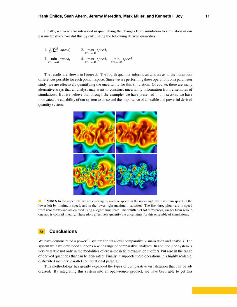
Finally, we were also interested in quantifying the changes from simulation to simulation in ourparameter study. We did this by calculating the following derived quantities:

1. 125 ∑25

i=1 speedi 2. maxi=1,...,25

speedi

3. mini=1,...,25

speedi 4. maxi=1,...,25

speedi− mini=1,...,25

speedi

The results are shown in Figure 5. The fourth quantity informs an analyst as to the maximumdifferences possible for each point in space. Since we are performing these operations on a parameterstudy, we are effectively quantifying the uncertainty for this simulation. Of course, there are manyalternative ways that an analyst may want to construct uncertainty information from ensembles ofsimulations. But we believe that through the examples we have presented in this section, we havemotivated the capability of our system to do so and the importance of a flexible and powerful derivedquantity system.

Figure 5 In the upper left, we are coloring by average speed, in the upper right by maximum speed, in thelower left by minimum speed, and in the lower right maximum variation. The first three plots vary in speedfrom zero to two and are colored using a logarithmic scale. The fourth plot (of differences) ranges from zero toone and is colored linearly. These plots effectively quantify the uncertainty for this ensemble of simulations.

6 Conclusions

We have demonstrated a powerful system for data-level comparative visualization and analysis. Thesystem we have developed supports a wide range of comparative analyses. In addition, the system isvery versatile not only in the modalities of cross-mesh field evaluation it offers, but also in the rangeof derived quantities that can be generated. Finally, it supports these operations in a highly scalable,distributed memory, parallel computational paradigm.

This methodology has greatly expanded the types of comparative visualization that can be ad-dressed. By integrating this system into an open-source product, we have been able to get this


technology in the hands of scientists and engineers. Future work will focus on the enhancements ofthese technologies to generate new comparative methods that impact their work.

References

1 Shen, Q., Pang, A., Uselton, S.: Data level comparison of wind tunnel and computational fluiddynamics data. In: Proceedings of the IEEE Visualization Conference, Los Alamitos, CA, IEEEComputer Society Press (1998) 415–418

2 de Leeuw, W.C., Pagendarm, H.G., Post, F.H., Walter, B.: Visual simulation of experimentaloil-flow visualization by spot noise images from numerical flow simulation. In: Visualization inScientific Computing. (1995) 135–148

3 Williams, P.L., Uselton, S.P.: Foundations for measuring volume rendering quality. TechnicalReport NAS/96-021, NASA Numerical Aerospace Simulation (1996)

4 Zhou, H., Chen, M., Webster, M.F.: Comparative evaluation of visualization and experimentalresults using image comparison metrics. In: Proceedings of the IEEE Visualization Conference,Washington, DC, IEEE Computer Society (2002)

5 Bavoil, L., Callahan, S., Crossno, P., Freire, J., Scheidegger, C., Silva, C., Vo, H.: VisTrails: en-abling interactive multiple-view visualizations. IEEE Transactions on Visualization and ComputerGraphics 12(6) (2005) 135–142

6 Batra, R.K., Hesselink, L.: Feature comparisons of 3-D vector fields using earth mover’s distance.In: Proceedings of the IEEE Visualization Conference. (1999) 105–114

7 Edelsbrunner, H., Harer, J., Natarajan, V., Pascucci, V.: Local and global comparison of continuousfunctions. In: Proceedings of the IEEE Visualization Conference. (October 2004) 275–280

8 Verma, V., Pang, A.: Comparative flow visualization. IEEE Transactions on Visualization andComputer Graphics 10(6) (2004) 609–624

9 Freitag, L., Urness, T.: Analyzing industrial furnace efficiency using comparative visualization in avirtual reality environment. Technical Report ANL/MCS-P744-0299, Argonne National Laboratory(1999)

10 Shen, Q., Uselton, S., Pang, A.: Comparison of wind tunnel experiments and computational fluiddynamics simulations. Journal of Visualization 6(1) (2003) 31–39

11 Sommer, O., Ertl, T.: Comparative visualization of instabilities in crash-worthiness simulations.In: Data Visualization 2001, Procceedings of EG/IEEE TCVG Symposium on Visualization. (2001)319–328

12 Abram, G., Treinish, L.A.: An extended data-flow architecture for data analysis and visualization.Research report RC 20001 (88338), IBM T. J. Watson Research Center, Yorktown Heights, NY(February 1995)

13 Computational Engineering International, Inc.: EnSight User Manual. (May 2003)14 Johnson, C., Parker, S., Weinstein, D.: Large-scale computational science applications using the

SCIRun problem solving environment. In: Proceedings of the 2000 ACM/IEEE conference onSupercomputing. (2000)

15 Moran, P.J., Henze, C.: Large field visualization with demand-driven calculation. In: Proceedingsof the IEEE Visualization Conference, Los Alamitos, CA, IEEE Computer Society Press (1999)27–33

16 McCormick, P.S., Inman, J., Ahrens, J.P., Hansen, C., Roth, G.: Scout: A hardware-acceleratedsystem for quantitatively driven visualization and analysis. In: Proceedings of the IEEE Visualiza-tion Conference, Washington, DC, IEEE Computer Society (2004) 171–178

17 Joy, K.I., Miller, M., Childs, H., Bethel, E.W., Clyne, J., Ostrouchov, G., Ahern, S.: Frameworks forvisualization at the extreme scale. In: Proceedings of SciDAC 2007, Journal of Physics: ConferenceSeries. Volume 78. (2007) 10pp


18 Childs, H., Miller, M.: Beyond meat grinders: An analysis framework addressing the scale andcomplexity of large data sets. In: SpringSim High Performance Computing Symposium (HPC2006). (2006) 181–186

19 Schroeder, W.J., Martin, K.M., Lorensen, W.E.: The design and implementation of an object-oriented toolkit for 3d graphics and visualization. In: Proceedings of the IEEE Visualization Con-ference, IEEE Computer Society Press (1996) 93–ff.

20 Childs, H., Brugger, E., Bonnell, K., Meredith, J., Miller, M., Whitlock, B., Max, N.: A contractbased system for large data visualization. In: Proceedings of the IEEE Visualization Conference.(2005)

21 Cormen, T., Leiserson, C., Rivest, R.: Introduction to Algorithms. McGraw-Hill Book Company(1990)

22 Callahan, S.P., Freire, J., Santos, E., Scheidegger, C.E., Silva, C.T., Vo, H.T.: Vistrails: visu-alization meets data management. In: SIGMOD ’06: Proceedings of the 2006 ACM SIGMODinternational conference on Management of data, New York, NY, USA, ACM (2006) 745–747

Documents

Comparative Visualization Using Cross-Mesh Field Evaluations and