Embed Size (px)
Citation preview

COMPARING FIVE EMPIRICAL BIODATA SCORING METHODS
FOR PERSONNEL SELECTION
Mark J. Ramsay, B.A.
Thesis Prepared for the Degree of
MASTER OF SCIENCE
UNIVERSITY OF NORTH TEXAS
August 2002
APPROVED: Douglas Johnson, Committee Member and Major Professor Terry Halfhill, Committee Member and Major Professor Joe Huff, Committee Member and Major Professor Ernest Harrell, Chair of the Psychology Department C. Neal Tate, Dean of the Robert B. Toulouse School of
Graduate Studies

Ramsay, Mark J., Comparing Five Empirical Biodata Scoring Methods for
Personnel Selection. Master of Science (Industrial Psychology), August 2002, 103 pp.,
8 tables, 3 appendices, references, 91 titles.
A biodata based personnel selection measure was created to improve the retention
rate of Catalog Telemarketing Representatives at a major U.S. retail company. Five
separate empirical biodata scoring methods were compared to examine their usefulness in
predicting retention and reducing adverse impact. The Mean Standardized Criterion
Method, the Option Criterion Correlation Method, Horizontal Percentage Method,
Vertical Percentage Method, and Weighted Application Blank Method using England’s
(1971) Assigned Weights were employed. The study showed that when using
generalizable biodata items, all methods, except the Weighted Application Blank
Method, were similar in their ability to discriminate between low and high retention
employees and produced similar low adverse impact effects. The Weighted Application
Blank Method did not discriminate between the low and high retention employees.

ii
TABLE OF CONTENTS Page
LIST OF TABLES… .… … … … … … … … … … … … … … … … … … … … … … … … .… ...iii Chapter
1. INTRODUCTION… … … … … … … … … … … … … … … … … … … … … ..… 1 What is Biodata? Assumptions of Biodata Types of Scaling Procedures Lack of Use of Biodata Benefits of Biodata Concerns about Biodata Summary
2. BIODATA STUDY… … ...… .… … … … … … … … … … … … … … … … … ..37 Rationale for Using Biodata and Hypotheses for the Study Method Results Discussion
APPENDIX A… … … … … … … … … … … … … … … … … … … … … … … … … … … … … 61 APPENDIX B… … … … … … … … … … … … … … … … … … … … … … … … … … … … … 83 APPENDIX C… … … … … … … … … … … … … … … … … … … … … … … … … … … … … 85 REFERENCES… … … … … … … … … … … … … … … … … … … … … … … … … … … ..… 92

iii
LIST OF TABLES
Table Page 1. Mount et al’s (2000) Four Different Biodata Scales and How They Correlate with Big
Five Factors … … … … … … … … … … … … … … … … … … … … … .… … … .… … .13-14 2. List of Criterion Measures Biodata Predicts and Their Validities… … … … … … ..15-16 3. Gender and Race Selection Percentage Rates of the Holdout Sample for each of the
Four Scoring Method… … … … … … … … … … … … … … … … … … … … … … … ..49-50 4. Comparison of Mean Retention Rates of the Holdout Criterion Groups for each of the
Four Scoring Methods… … … … … … … … … … … … … … … … … … … … … … … 50-51 5. Correlation Matrix Between the Four Scoring Methods and Retention Using the
Holdout Sample ..................................................................................................... ..51
6. Gender and Race Selection Percentage Rates of the Holdout Sample for each of the Four Scoring Methods After Eliminating Adverse Impact Items ............................ ..53
7. Comparison of Mean Retention Rates of the Holdout Criterion Groups for each of the
Four Scoring Methods After Eliminating Adverse Impact Items ............................ ..54 8. Correlation Matrix Between the Four Scoring Methods and Retention Using the
Holdout Sample After Eliminating Adverse Impact Items...................................... ..55

1
CHAPTER 1
INTRODUCTION
What is Biodata?
Selecting the right people for the right job is becoming increasingly more
important for organizations. Due to increased global competition and an increase in
technology, customers can get goods or services from numerous companies throughout
the world. As a result, the one way organizations can gain a competitive advantage over
its rivals is through their employees, their intellectual capital. In the age of information,
the employees are the ones who hold the company together, retain customers, and help
the company grow with their creativity. Therefore, personnel selection is more critical
than ever in today’s business world. Selecting the wrong person for the job can be costly.
Using a complicated and expensive selection process while a cheaper and equally
effective one is available can also be very detrimental to the success of an organization.
One selection method that is inexpensive, compared to other methods, and has good
predictive validity for job success is biodata (Hunter, 1986; Hunter & Hunter, 1984;
Reilly & Chao, 1982; Schmitt, Gooding, Noe, & Kirsch, 1984).
Biodata are questions, usually in multiple-choice format, that measure one or
more criteria that human resource professionals use to predict future applicant
performance. Biodata comes from two basic information sources. One source is people’s

2
past interests and experiences, and the other is people’s opinions or attitudes as a
consequence of those experiences (Dickinson & Ineson, 1993). Hence, biodata ask
applicants questions about their personal background, past life, work experiences and
about their opinions, values, beliefs and attitudes of the aforementioned areas.
Mael (1991) identified 10 dimensions of biodata. The 10 dimensions are:
? Historical vs. Hypothetical – whether an item asks about past or future
situations
Examples: Historical: “Have you worked in a team environment?”
Hypothetical: “How well would you work in a team environment?”
? Objective vs. Subjective – whether an item asks to recall facts or asks for
opinions
Examples: Objective: “How many accounts did you handle last year?”
Subjective: “Would you describe yourself as a good accountant?”
? First vs. Second Hand – whether an item asks about observations of yourself
or other people’s perceptions of you
Examples: First Hand: “Do you communicate well with your employers?”
Second Hand: “How would others describe your communication
skills?”
? Verifiable vs. Non Verifiable – whether human resource professionals can or
cannot check the item’s answer for accuracy
Examples: Verifiable: ”What was your last employee rating?”
Non-Verifiable: “Are you a hard worker?”

3
? External vs. Internal: whether an item asks about observable events
Examples: External: “When you were in school, how much time did you
spend studying?”
Internal: “What best describes your feeling, when you last worked
in a team environment?”
? Job Relevant vs. Non Job Relevant – whether an item asks about job related
aspects or not
Examples: Job Relevant: “In your last job, how often did you work with
computers?”
Non-Job Relevant: “How many times do you go to the movies in a
week?”
? Discrete vs. General – whether an item asks about a single particular event or
not
Example: Discrete: “How old were you when you first had a job?”
General: “While growing up what activities did you enjoy most?”
? Controllability vs. Non Controllability – extent to which items ask about
experiences subjects had direct control over. Non-control questions usually
ask about applicants’ demographics or parent’s behavior.
Example: Control: “When you were in school, how much time did you spend
studying?”
No Control: “What was the population of the city you grew up in?”

4
? Equal Accessibility vs. Unequal Accessibility – extent to which the question is
relevant to or applies to all subjects. Some questions might not apply to all the
subjects because the subjects did not have an opportunity to do or have access
to use what the question is asking.
Example: Equal Accessibility – “Do you communicate well with others?”
Unequal Accessibility – “How much time did you spend on the
Internet per week while in high school?”
? Invasiveness vs. Non-Invasiveness – extent to which the question is found
offensive by the subject because it asks about private or confidential
information. Subjects usually find questions about marital status and political
or religious affiliation to be offensive.
Example: Invasive – “What is your marital status?”
Non-Invasive – “How often did you work in a team environment at
your last job?”
Assumptions of Biodata
The rationale underlying the use of biodata for personnel selection comes from
several assumptions. The main assumption is that the best predictor of one’s future
performance is one’s past performance (Mumford & Owens, 1987). Social Identity
Theory (SIT) links to this assumption and provides a rationale for it. The SIT states that a
person’s past experiences and values will help typify how the person will act in new
social situations and group settings like organizations (Mael & Ashforth, 1995). To create
order in their society, individuals identify their places and other people’s places in

5
society. They do this by using race, skills, interests, backgrounds etc. to categorize
themselves and others into groups or affiliations. Once in these groups, individuals take
on the characteristics of these groups. Many groups and affiliations actually instill new
values and attitudes into their members in which the members then internalize and use
long after leaving their group to make decisions on how to act and what to do. Social
Identity Theory argues that biodata reflects a person’s past experiences, which in turn,
affect what values, a person internalizes and hence how a person will act in the future.
For example, background questions about what past clubs, interests, or societies a person
was a member of may be important in determining how successful the person is on the
job (Mael & Ashforth, 1995). An example of a successful predictor of success in flight
school for the Air Force during World War II was “Did you ever build a model airplane
that flew” (Cureton, 1965). This question was successful because people who built model
airplanes that flew probably enjoyed working with and learning about airplanes. Hence
they had a better understanding of how planes work and therefore did better in flight
school.
O’Reilly and Chatman (1986) showed that internalization, compliance, and
identification with organizational values relates to prosocial behaviors like intent to stay,
and low turnover. The Organizational Commitment Survey, measures commitment by
looking at the individual’s congruence with organizational goals and values, and
willingness to remain a member (Ashforth & Mael, 1989). So if a person’s values do not
fit with the organization’s values, organizational commitment can be low and the person
might not perform as well. Biodata questions are useful in these areas because they can
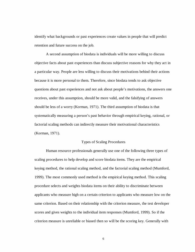
6
identify what backgrounds or past experiences create values in people that will predict
retention and future success on the job.
A second assumption of biodata is individuals will be more willing to discuss
objective facts about past experiences than discuss subjective reasons for why they act in
a particular way. People are less willing to discuss their motivations behind their actions
because it is more personal to them. Therefore, since biodata tends to ask objective
questions about past experiences and not ask about people’s motivations, the answers one
receives, under this assumption, should be more valid, and the falsifying of answers
should be less of a worry (Korman, 1971). The third assumption of biodata is that
systematically measuring a person’s past behavior through empirical keying, rational, or
factorial scaling methods can indirectly measure their motivational characteristics
(Korman, 1971).
Types of Scaling Procedures
Human resource professionals generally use one of the following three types of
scaling procedures to help develop and score biodata items. They are the empirical
keying method, the rational scaling method, and the factorial scaling method (Mumford,
1999). The most commonly used method is the empirical keying method. This scaling
procedure selects and weights biodata items on their ability to discriminate between
applicants who measure high on a certain criterion to applicants who measure low on the
same criterion. Based on their relationship with the criterion measure, the test developer
scores and gives weights to the individual item responses (Mumford, 1999). So if the
criterion measure is unreliable or biased then so will be the scoring key. Generally with

7
the empirical keying method, understanding how human theory or psychology explains
the relationship between the item responses and the criteria is not a priority, when human
resource professionals develop the biodata items. Instead statistical analysis of how well
the item responses predict the criterion justifies the relationship. Once statistical analysis
identifies the relationship between the item and criterion, then the human resource
professionals will go back and try and explain the relationship with underlying broader
theory or constructs if need be.
The empirical keying method also has several different types of scoring methods
to weight the predictors or the individual item responses. Five commonly used types are
the Horizontal Percentage Method (HPM) (Stead & Shartle, 1940), the Vertical
Percentage Method (VPM) using Strong’s Net Weights (England, 1971), the Option
Criterion Correlation Method (OCC) (Lecznar & Dailey, 1950), the Mean Standardized
Criterion Method (MSC) (Mitchell, 1994), and England’s (1971) Weighted Application
Blank Method (WAB) using his Assigned Weights. England (1961) suggested that the
HPM, VPM, and WAB (the scoring methods that use percentages) would produce more
stable weights than other types of empirical scoring methods. However, Mumford and
Owens (1987) suggested that correlation and regression methods would create better
weights after cross-validation occurs. But not much reported research exists comparing
these different empirical scoring methods (Mitchell, 1994).
Two of the scaling procedures that can help the practitioner develop biodata items
with a more logical link to the construct and help them explain better the relationship
between the biodata item and the criterion prediction are the rational and factorial scaling
8
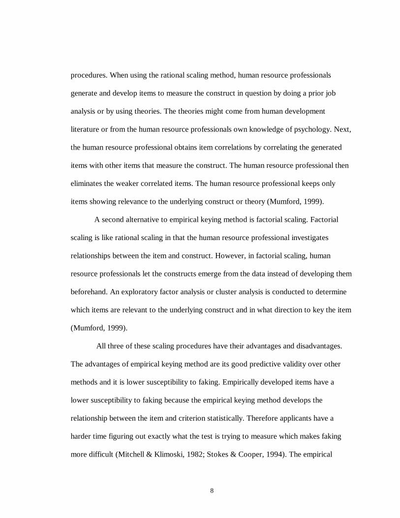
procedures. When using the rational scaling method, human resource professionals
generate and develop items to measure the construct in question by doing a prior job
analysis or by using theories. The theories might come from human development
literature or from the human resource professionals own knowledge of psychology. Next,
the human resource professional obtains item correlations by correlating the generated
items with other items that measure the construct. The human resource professional then
eliminates the weaker correlated items. The human resource professional keeps only
items showing relevance to the underlying construct or theory (Mumford, 1999).
A second alternative to empirical keying method is factorial scaling. Factorial
scaling is like rational scaling in that the human resource professional investigates
relationships between the item and construct. However, in factorial scaling, human
resource professionals let the constructs emerge from the data instead of developing them
beforehand. An exploratory factor analysis or cluster analysis is conducted to determine
which items are relevant to the underlying construct and in what direction to key the item
(Mumford, 1999).
All three of these scaling procedures have their advantages and disadvantages.
The advantages of empirical keying method are its good predictive validity over other
methods and it is lower susceptibility to faking. Empirically developed items have a
lower susceptibility to faking because the empirical keying method develops the
relationship between the item and criterion statistically. Therefore applicants have a
harder time figuring out exactly what the test is trying to measure which makes faking
more difficult (Mitchell & Klimoski, 1982; Stokes & Cooper, 1994). The empirical

9
method also takes less time and money to create than the rational or factorial scaling
method (Mitchell & Klimoski, 1982). This method can also identify relationships
between items and constructs that would be difficult to discover or see through job
analysis, the rational scaling method, or factorial scaling method. Of course the downside
is the time it might take discovering how to explain the relationship. Other negatives of
empirical keying, besides the lack of understanding it gives to item and construct
relationship, is the lack of generalizability if the practitioner does not develop the sample
and items well. Finally, the face validity is also lower as a result of using less objective
and less transparent items.
The positives of the rational scaling method are it provides a greater
understanding of the relationship between item and construct (i.e. greater legal
defensibility) and a greater generalizability of the selection tool (Mumford, 1999). This
method can also use smaller samples to validate it (Allworth, 1999).
The rational scaling method also has several negatives. Because the rational
method is theoretically based and the relationship is more logical between the item and
construct, the items are easier to fake or to choose the socially desirable answer
(Mumford, 1999). Second, the predictive validity of the rational method is not as strong
as the empirically keyed method (Allworth, 1999; Mael & Hirsch, 1993, Mitchell &
Klimoski, 1982). The rational method is also more complex and costly to use than the
empirical method.
The advantage of the factorial scaling method is it allows human resource
professionals to see how constructs emerge in a specific population (Mumford, 1999).
10
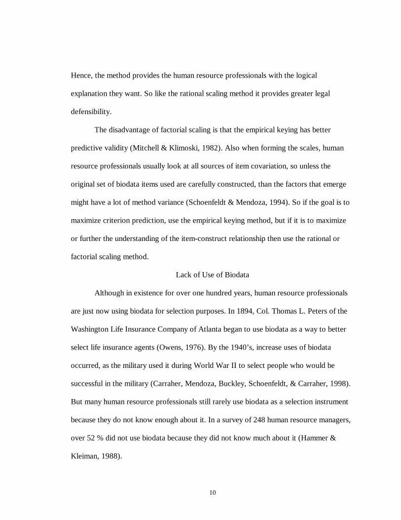
Hence, the method provides the human resource professionals with the logical
explanation they want. So like the rational scaling method it provides greater legal
defensibility.
The disadvantage of factorial scaling is that the empirical keying has better
predictive validity (Mitchell & Klimoski, 1982). Also when forming the scales, human
resource professionals usually look at all sources of item covariation, so unless the
original set of biodata items used are carefully constructed, than the factors that emerge
might have a lot of method variance (Schoenfeldt & Mendoza, 1994). So if the goal is to
maximize criterion prediction, use the empirical keying method, but if it is to maximize
or further the understanding of the item-construct relationship then use the rational or
factorial scaling method.
Lack of Use of Biodata
Although in existence for over one hundred years, human resource professionals
are just now using biodata for selection purposes. In 1894, Col. Thomas L. Peters of the
Washington Life Insurance Company of Atlanta began to use biodata as a way to better
select life insurance agents (Owens, 1976). By the 1940’s, increase uses of biodata
occurred, as the military used it during World War II to select people who would be
successful in the military (Carraher, Mendoza, Buckley, Schoenfeldt, & Carraher, 1998).
But many human resource professionals still rarely use biodata as a selection instrument
because they do not know enough about it. In a survey of 248 human resource managers,
over 52 % did not use biodata because they did not know much about it (Hammer &
Kleiman, 1988).

11
Even though LIMRA (the Life Insurance Marketing and Research Association)
has prevalently used biodata to successfully select insurance agents since 1930, other
industries do not use biodata for several reasons (McManus & Kelly, 1999). In Europe,
organizations also seldom use biodata as a selection tool (Wilkinson, 1997). A main
reason for the lack of use is the lack of familiarity with the technique (Hammer &
Kleiman, 1988). Many organizations are unfamiliar with the benefits of biodata over
other selection tools and have concerns with issues of generalizability, validity, adverse
impact, faking of answers, the invasiveness of the questions, using job incumbents or job
applicants to develop the biodata key, and dustbowl empiricism or the rationale behind
the construction of the items.
Benefits of Biodata
Biodata has several benefits as a selection instrument, especially in comparison to
the interview, the most commonly used and preferred selection method (Shackleton &
Newell, 1991; Smith & Pratt, 1996). First, biodata can quickly obtain the same type of
information one might get from a selection interview. Unlike the interview process,
biodata can gather information on hundreds of candidates at once. Hence, biodata is less
costly than the interview method and uses fewer employee resources (Smith & Pratt,
1996). Biodata also has the additional advantage that human resource professionals can
empirically score and use the information as a determinant in selection. Not only can
biodata help replace the interview process and still obtain similar information, but it can
also help improve selection decisions, especially over the unstructured interview. When
constructed properly, Cascio (1992) showed that biodata could be more effective than the

12
interview when predicting future job performance. The empirical scoring procedure can
also be an important step in eliminating non-relevant and non-job related questions,
which helps reduce adverse impact. However, human resource professionals need to take
additional steps to ensure development of a fair and legal selection test. Through the
empirical, rational, or factorial scoring techniques, biodata can also help managers
understand and identify better what applicant values or experiences will make for an ideal
employee (Morrison, 1994). Even though biodata has some advantages over the
interview, organizations can best improve their selection process by using both of them
together.
Biodata is also very beneficial and useful for certain jobs more than others.
Biodata is more beneficial for jobs in which organizations ask employees to perform
repetitive or similar attributes (Mitchell, 1994). Job analysis can easily be done on jobs
with repetitive activities making the process of coming up with job related questions
much easier. Also jobs where human resource personnel have direct access to personnel
records to obtain and verify biographical information make biodata very useful and easy
to use. Biodata is also very beneficial for jobs that have high turnover rate or require long
costly training. Biodata can decrease the turnover rate and hence decrease training cost
and time. Finally, biodata is very useful prescreening technique to use when the job has a
large number of applicants and organizations want to cut down on the number of
interviews and testing they have to do (Mitchell, 1994).
Biodata also provides incremental validity when used in conjunction with general
mental ability (GMA) and personality tests. GMA tests are good predictors of job

13
performance, especially for very complex jobs (Mount, Witt, & Barrick, 2000). GMA is
the best predictor of job-related learning and GMA’s criterion-related validity is stronger
than any other single selection method (Hunter, 1986; Hunter & Schmidt, 1996; Ree &
Earles, 1992; Schmidt & Hunter, 1981). Biodata can help improve the validity of a
GMA-based selection measure (Mael & Ashforth, 1995). In fact in one instance, Dean
and Russell (1998) found that biodata was actually a better predictor of FAA air traffic
controller’s training performance than GMA measures. Even though GMA tests are good
predictors of job performance, they cannot account for all of the variance in the criterion.
Biodata can add incremental validity. Biodata can also add incremental validity to
personality measures, like the Five Factor Model or the Big Five (Mount et al., 2000;
McManus & Kelly, 1999). Biodata relates to GMA (r. = .50) and somewhat with
personality measures (Chait, Carraher, & Buckley, 2000; Schmidt, 1998). Table 1 shows
Mount et al.’s (2000) four different biodata scales and how they correlated differently
with the Big Five Factors.
Table 1.
Mount et al’s (2000) Four Different Biodata Scales and How They Correlate with Big
Five Factors
Big Five Factors
Type of Biodata Scale C E A ES O
Work Habit Biodata Scale .28 -.22 .01 .03 -.02
Problem Solving Abilities Biodata Scale .43 .48 .01 .35 .54
Interpersonal Relationship Biodata Scale .35 .13 .17 .39 .34

14
Situation Perseverance Biodata Scale .13 -.12 .13 .24 .14
Note. C = Conscientiousness, E = Extraversion, A = Agreeableness, ES = Emotional
Stability, O = Openness. Values given are r values.
Hence, biodata may measure indirectly mental ability and the Big Five personality factors
(Chait et al., 2000; Schmidt & Hunter, 1998).
Biodata can account for some of the variance that GMA measures and personality
measures cannot because biodata measures different criteria and is usually constructed
differently. First of all, biodata items usually measure a broader area of skills, attributes,
and traits than GMA or personality items. While GMA measures critical thinking and
analytical skills, biodata can also identify other traits or skills that a person has that might
be good indicators of future performance (Mount et al., 2000). GMA tends to measure an
applicant’s maximum performance or an applicant’s level at peak performance while
biodata looks to measure an applicant’s typical performance (Allworth, 1999).
Personality selection tools use items that focus on how applicants respond to general
situations, while biodata items tend to focus on specific situations and experiences.
Therefore biodata items can gain different information, because biodata items ask about
events or experiences that have actually taken place. Hence the applicant’s physical
abilities, perceptual abilities, and other situational factors and constraints of the specific
event in question will influence the applicant’s response to the biodata questions
(McManus & Kelly, 1999).
Biodata might also account for some of the unexplained variance because human
resource professionals generally construct biodata differently than GMA and personality

15
measures. GMA and personality measures usually use a construct-oriented approach
while biodata usually uses a criterion-related approach (but biodata can be designed to
measure a particular construct). GMA and personality tests are designed to measure
certain skills or traits that relate to a construct field like conscientiousness or analytical
ability. They are not designed to predict a criterion for a specific job as are biodata tests.
Biodata uses items based on their empirical relationship to the criterion for a specific job.
The items are designed to differentiate applicants on the criterion measure. So GMA and
personality selection tools will generalize to other jobs that have similar constructs.
Biodata selection tools will generalize to other jobs that use similar criterion to predict
job performance, retention, etc. (Mount et al., 2000).
Another benefit of biodata is it predicts a multitude of job criterion measures to
differentiate applicants and predict future job performance. Table 2 shows a number of
criterion measures biodata has predicted and their corresponding validity coefficients:
Table 2.
List of Criterion Measures that Biodata Predicts and Their Validities
Criterion Measure
Author(s) r K N
Reilly & Chao (1982)
.32 13 5,721 Tenure
Hunter & Hunter (1984)
.26 23 10,800
Reilly & Chao (1982)
.39 3 569 Training success
Hunter & Hunter (1984)
.30 11 6,139
Performance ratings
Schmitt et al. (1984);
.32 29 3,998

16
Hunter & Hunter, 1984
.37 12 4,429
Promotions Hunter & Hunter, 1984
.26 17 9,024
Achievement Schmitt et al. (1984)
.23 9 1,744
Sales performance
Mumford & Owen (1987)
.35 17 -
Productivity of scientists & Engineers
Reilly & Chao (1982)
.43 5 563
Military training Reilly & Chao (1982)
.39 3 569
Leadership Mael & Hirsch (1993)
.28-.45 1 various
Performance of managers
Mumford & Owens (1987)
.35 21 -
Team performance
Mitchell (1992) .27 1 117
Clerical problem solving
Mount et al. (2000)
.37 1 146
Clerical work habits
Mount et al. (2000)
.33 1 146
Note. K = Number of studies
Research showed that biodata also differentiates between groups like white-collar
criminals and non-criminal white-collar employees, between quality or ‘good’ hotel
employees and ‘bad’ hotel employees, and between accident-prone people and non-
accident-prone people (Collins & Schmidt, 1993; Denning, 1983 as cited in Stokes &
Cooper, 1994; Dickinson & Ineson, 1993).
Biodata also can have good utility as a selection measure when human resource
professionals develop it correctly. The cost and manpower it takes to develop a biodata
selection tool is far less when compared to assessment centers or work samples (Hunter,
1986). Once developed, it is efficient because human resource professionals can
17
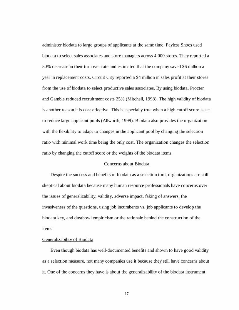
administer biodata to large groups of applicants at the same time. Payless Shoes used
biodata to select sales associates and store managers across 4,000 stores. They reported a
50% decrease in their turnover rate and estimated that the company saved $6 million a
year in replacement costs. Circuit City reported a $4 million in sales profit at their stores
from the use of biodata to select productive sales associates. By using biodata, Procter
and Gamble reduced recruitment costs 25% (Mitchell, 1998). The high validity of biodata
is another reason it is cost effective. This is especially true when a high cutoff score is set
to reduce large applicant pools (Allworth, 1999). Biodata also provides the organization
with the flexibility to adapt to changes in the applicant pool by changing the selection
ratio with minimal work time being the only cost. The organization changes the selection
ratio by changing the cutoff score or the weights of the biodata items.
Concerns about Biodata
Despite the success and benefits of biodata as a selection tool, organizations are still
skeptical about biodata because many human resource professionals have concerns over
the issues of generalizability, validity, adverse impact, faking of answers, the
invasiveness of the questions, using job incumbents vs. job applicants to develop the
biodata key, and dustbowl empiricism or the rationale behind the construction of the
items.
Generalizability of Biodata
Even though biodata has well-documented benefits and shown to have good validity
as a selection measure, not many companies use it because they still have concerns about
it. One of the concerns they have is about the generalizability of the biodata instrument.

18
Can they use biodata that human resource professionals do not specifically design for
their organization and the job in question. This concerns many companies because they
do not have the time or number of employees to develop their own biodata instrument,
especially for the smaller companies where it is just not feasible for them to develop their
own selection instrument (Wilkinson, 1997). One reason this concern developed is
because early research on biodata showed that it was situation specific or not
generalizable (Dreher & Sackett, 1983; Hunter & Hunter, 1984; Thayer, 1977). Thayer
(1977) proposed that biodata was not generalizable because factors like age, race, sex,
criterion measure used, and organizational variables act as moderators. For example,
Schmidt, Hunter, and Caplan (1981) found that empirically keyed biodata measures did
not generalize across 2 petroleum organizations. Dreher and Sackett (1983) suggested
that even though biodata has good validity, keying biodata items specifically for one
organization prevented them from being generalizable to other organizations.
However, more recent research opposed past findings and showed that biodata
can be generalizable. Rothstein, Schmidt, Erwin, Owens, and Sparks (1990) found that
using a large sample from multiple organizations with job-relevant biodata items
produced a generalizable biodata selection instrument with a validity of r = .32. The
biodata instrument generalized across organizations and demographic variables (like race,
gender, age, education, work experience, and company tenure). A later study by Carlson,
Scullen, Schmidt, Rothstein, and Erwin (1999) showed that even when using a single
organization as the sample, a biodata selection instrument produced generalizable
validities across multi-organizations and industries. Constaza and Mumford (1993)

19
showed that constructing biodata instruments using the rational scaling procedure led to
generalizability across ethnic and gender groups (as cited in Mumford, 1999). Cassens
(1966) sampled managers from both North and Latin America and found that factorial
design biodata items also generalized across cultures (as cited in Mumford, 1999).
Brown, Corrigan, Stout, and Dalessio (1987) tested the generalizability of empirically
keyed biodata items by using a sample of life insurance salesman from the U.S., Canada,
and South Africa. They obtained validities of r = .11 - .36 and showed that empirically
keyed biodata items can generalize across cultures. Biodata items can also generalize
from job to job when the biodata items emphasize core activities of the jobs and not the
specialty areas of the job (Campbell, Dunnette, Lawler, and Weick, 1970).
The differences in the construction of the biodata tests were the major reason why
these latter studies contradicted the earlier ones and showed biodata to be generalizable.
Earlier, studies tended to use a specific criterion for a specific job in a specific
organization to develop and key the biodata items (Mount et al., 2000). Hence, this
limited the biodata’s generalizability to other jobs and organizations , but this usually
improved the biodata’s predictive validity for that specific job and organization.
Generalizable biodata tests usually have one or more of the following characteristics.
First, generalizable biodata tests focus on core criterion measures or attributes that focus
on many jobs and are not job specific or situation specific. Rothstein et al. (1990) and
Carlson et al. (1999) demonstrated this by not focusing on functional specialties in their
studies. Research also showed that ability factors tend to generalize the most across
different jobs. Biodata tests that focus on these ability factors tended to generalize as well
20
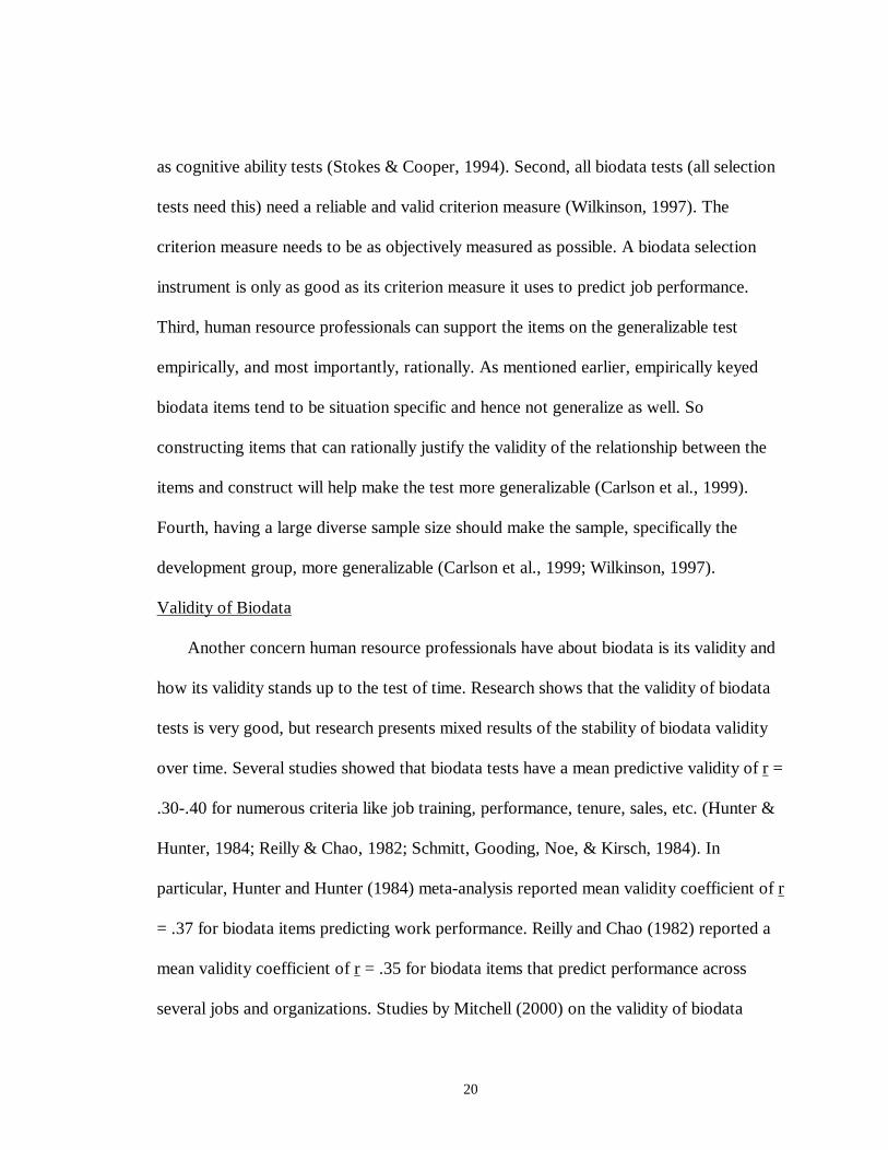
as cognitive ability tests (Stokes & Cooper, 1994). Second, all biodata tests (all selection
tests need this) need a reliable and valid criterion measure (Wilkinson, 1997). The
criterion measure needs to be as objectively measured as possible. A biodata selection
instrument is only as good as its criterion measure it uses to predict job performance.
Third, human resource professionals can support the items on the generalizable test
empirically, and most importantly, rationally. As mentioned earlier, empirically keyed
biodata items tend to be situation specific and hence not generalize as well. So
constructing items that can rationally justify the validity of the relationship between the
items and construct will help make the test more generalizable (Carlson et al., 1999).
Fourth, having a large diverse sample size should make the sample, specifically the
development group, more generalizable (Carlson et al., 1999; Wilkinson, 1997).
Validity of Biodata
Another concern human resource professionals have about biodata is its validity and
how its validity stands up to the test of time. Research shows that the validity of biodata
tests is very good, but research presents mixed results of the stability of biodata validity
over time. Several studies showed that biodata tests have a mean predictive validity of r =
.30-.40 for numerous criteria like job training, performance, tenure, sales, etc. (Hunter &
Hunter, 1984; Reilly & Chao, 1982; Schmitt, Gooding, Noe, & Kirsch, 1984). In
particular, Hunter and Hunter (1984) meta-analysis reported mean validity coefficient of r
= .37 for biodata items predicting work performance. Reilly and Chao (1982) reported a
mean validity coefficient of r = .35 for biodata items that predict performance across
several jobs and organizations. Studies by Mitchell (2000) on the validity of biodata

21
items to predict 3 criteria of successful performance in fire fighting produced validities of
r = .30 - .39. Compared to the validities of other selection measures, the mean validity of
biodata makes it one of the higher validity selection methods. When predicting job
performance, GMA tests have a validity of r = .51 (Hunter, 1980), structured and
unstructured interviews have a validity of r = .51 and r = .38, respectively (Huffcut, Roth,
& McDaniel, 1996; McDaniel, Whetzel, Schmidt, & Mauer, 1994), conscientiousness
tests have a validity of r = .31 (Mount & Barrick, 1995), and Hunter and Hunter (1984)
showed reference checks have a validity of r = .26 and academic achievement has a
validity of r = .10. So biodata stacks up well when comparing predictive validities with
other selection tests.
Research examining the stability of biodata validity is limited and not clear-cut.
Wernimont (1962) demonstrated that the validity of a biodata test, predicting tenure,
dropped from r = .74 to r = .38 after 3 years and to r = .07 after 5 years. However, making
changes to the scoring key and changing some of the items brought the validity back up
to r = .39. Other research also supported the fact that validity of biodata items decay over
time, specifically with empirically keying and item weighting (Hogan, 1994; Mitchell &
Klimoski, 1982).
However, a few studies opposed these findings. Brown (1978) showed that biodata
selection test for life insurance agents did not lose significant validity over a 38-year
period. Brown contended that ensuring the confidentiality of the scoring key and having a
large development sample were important steps to maintaining the stability of the biodata
validity over time. Hunter and Hunter (1984) refuted this claim, and said Brown was

22
looking at the statistical significance of the observed validities over time and not the
actual validity coefficients. The actual validity coefficients did decay over time. Reiter-
Palmon (1986) demonstrated that factorial designed biodata items’ validity were stable
over a 25-year period (as cited in Mumford, 1999). Barrett, Alexander, and Doverspike
(1992) and Rothstein et al. (1990) also provided support for stability of biodata validity.
These studies possibly showed stability because they focused on some of the previous
factors mentioned that help make biodata tests generalizable like focusing on the core
criteria of jobs that do not change over time and using items with good rationale to
explain the item relationship with the construct.
Overall though, biodata shows a tendency to decay over time. Therefore, human
resource professionals need to reevaluate biodata tests and reweight the scoring keys
every 2 to 3 years (Reilly & Chao, 1982; Thayer, 1977; Wernimount, 1962).
Several reasons exist why the validity of biodata items decay over time. The first
is the predictors for the job performance might change (i.e. skills for the job) or the
organization might change the way they measure the criterion, which will impact the
scoring key and weighting system. Second, the population the human resource
professionals develop the biodata for might change which can also hurt the scoring key.
Third, any changes in the organizations culture or in organization policies may also
change the effectiveness of the biodata key (Hogan, 1994).
Also several factors can hurt the validity by resulting in range restriction. First,
the hiring decisions made from the biodata test will usually lead to range restriction on
the criterion and decreases in estimates of concurrent validity. Secondly, when hiring

23
managers have access to the scores of the job applicants, the manager’s job performance
expectations might affect how the manager treats and helps the employees. Employees
who score low might get more training and support while employees who score high
might get less help. The result is the difference between the job performance of the
employees who score high on the biodata and those that score low will narrow and in the
future determining if the biodata test discriminates between good and bad performers will
be harder (Brown, 1978; Brumback, 1969). The final factor that can affect the validity is
the confidentiality of the scoring key like Brown (1978) mentioned. If hiring managers
know the correct answers to pass an applicant, they might tell the applicant how to
answer, especially if the manager is in dire need of filling job vacancies. As a result,
incorrectly using the biodata test will lower its validity (Mitchell, 1987 as cited in Hogan,
1994). So based on these factors biodata tests that predict future performance in non job
settings like for academic success might retain its validity longer since the external
factors that affect the job market will not affect these types of test as much (Melamed,
1992).
Adverse Impact of Biodata
Third area of concern human resource professionals have about biodata is the
potential adverse impact it might have (Hammer & Kleiman, 1988). People are concerned
whether biodata tests predict minority job performance as well as it does for non-minority
applicants and does it result in equal hiring rates for all races, ethnicity, age, and gender.
Human resource professionals’ concerns about adverse impact might be grounded in the
fact that they wonder how a test that uses people’s past performance and history to

24
predict future performance can treat people of different races and gender the same.
Obviously people of different races and gender usually do not experience the same
situations or even have the opportunity to experience the same situations.
However other researchers offer possible reasons why biodata might minimize
adverse impact. One reason biodata might minimize adverse impact is because it has
predictor-criterion related validity. This means that biodata unlike cognitive ability tests
measures what people do under typical circumstances to predict how that person will
typically perform in future situations (Mitchell, 1994). Mental ability tests measure
people’s maximum performance, and many people just do not test well under those
situations. Also ability tests have one right answer, biodata tests do not. In fact certain
biodata items have several ‘right’ or ‘wrong’ answers. As a result, biodata has
equipollence (Mitchell, 1990). This means that people with different personalities and
different backgrounds can be just as successful when taking the selection test (Mitchell,
1994). A second possible reason biodata might limit adverse impact is its items focus on
the person and his/her behavior in the context of his/her life, and does not compare it to
other individuals. Therefore this eliminates differences between applicants’ backgrounds.
For instance, biodata does not treat people differently who respond they do well in a
public school to people who respond they do well in a private school. A final theory why
biodata might minimize adverse impact is that biodata measures or focuses on people’s
motivation, efforts, and interests and not just on their mental ability (Mumford, 1999).
Research on adverse impact of biodata supports these theories by demonstrating
little or no adverse impact of biodata. Reilly and Chao (1982) showed that biodata is one
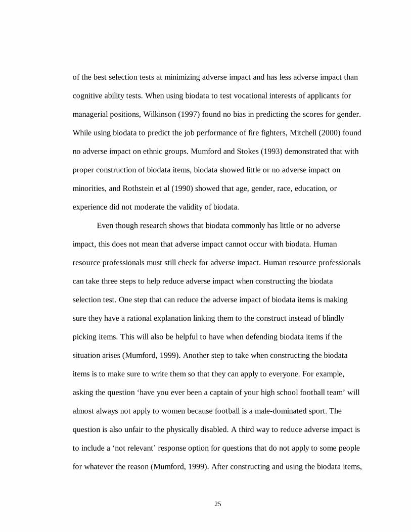
25
of the best selection tests at minimizing adverse impact and has less adverse impact than
cognitive ability tests. When using biodata to test vocational interests of applicants for
managerial positions, Wilkinson (1997) found no bias in predicting the scores for gender.
While using biodata to predict the job performance of fire fighters, Mitchell (2000) found
no adverse impact on ethnic groups. Mumford and Stokes (1993) demonstrated that with
proper construction of biodata items, biodata showed little or no adverse impact on
minorities, and Rothstein et al (1990) showed that age, gender, race, education, or
experience did not moderate the validity of biodata.
Even though research shows that biodata commonly has little or no adverse
impact, this does not mean that adverse impact cannot occur with biodata. Human
resource professionals must still check for adverse impact. Human resource professionals
can take three steps to help reduce adverse impact when constructing the biodata
selection test. One step that can reduce the adverse impact of biodata items is making
sure they have a rational explanation linking them to the construct instead of blindly
picking items. This will also be helpful to have when defending biodata items if the
situation arises (Mumford, 1999). Another step to take when constructing the biodata
items is to make sure to write them so that they can apply to everyone. For example,
asking the question ‘have you ever been a captain of your high school football team’ will
almost always not apply to women because football is a male-dominated sport. The
question is also unfair to the physically disabled. A third way to reduce adverse impact is
to include a ‘not relevant’ response option for questions that do not apply to some people
for whatever the reason (Mumford, 1999). After constructing and using the biodata items,

26
human resource professionals can screen and check to see if any items create adverse
impact. They can then remove the items that do cause adverse impact. Because removal
of some items might occur, creating a biodata selection test from a pool of items is
beneficial (Whitney & Schmidt, 1997 as cited in Allworth, 1999).
Invasiveness of Biodata
Some organizations do not use biodata because of concerns about applicants’
reactions to the selection test and whether some biodata questions might be too invasive
(Hammer & Kleiman, 1988). This is a legitimate concern for several reasons. First, a
selection test that does not seem fair, or relvent, or seems invasive might hurt the
attractiveness of the organization to a potential employee (Smither, Reilly, Millsap,
Pearlman, & Stoffey, 1993). If the applicants do not like the test they might go to another
company that treats them better during the recruiting and selection process. Losing
potential employees because of a selection test can become a serious problem in a tight
labor market. Second, if applicants perceive the test as unfair or not job related and the
organization does not hire them for the job, then lawsuit or litigation is more likely to
follow. So face validity is important for the selection test. Finally, if applicants do not
perceive the test as fair, they might not try as hard on the test. This may decrease the
validity and utility of the test (Smither et al., 1993). So the reactions applicants have to
the test are important to consider.
Research evidence on the invasiveness issue is conflicting. According to a Bureau
of National Affairs survey, invasiveness of biodata items was a major reason why only
4% of the personnel specialists use biodata (Mael, Connerley, & Morath, 1996). Hammer
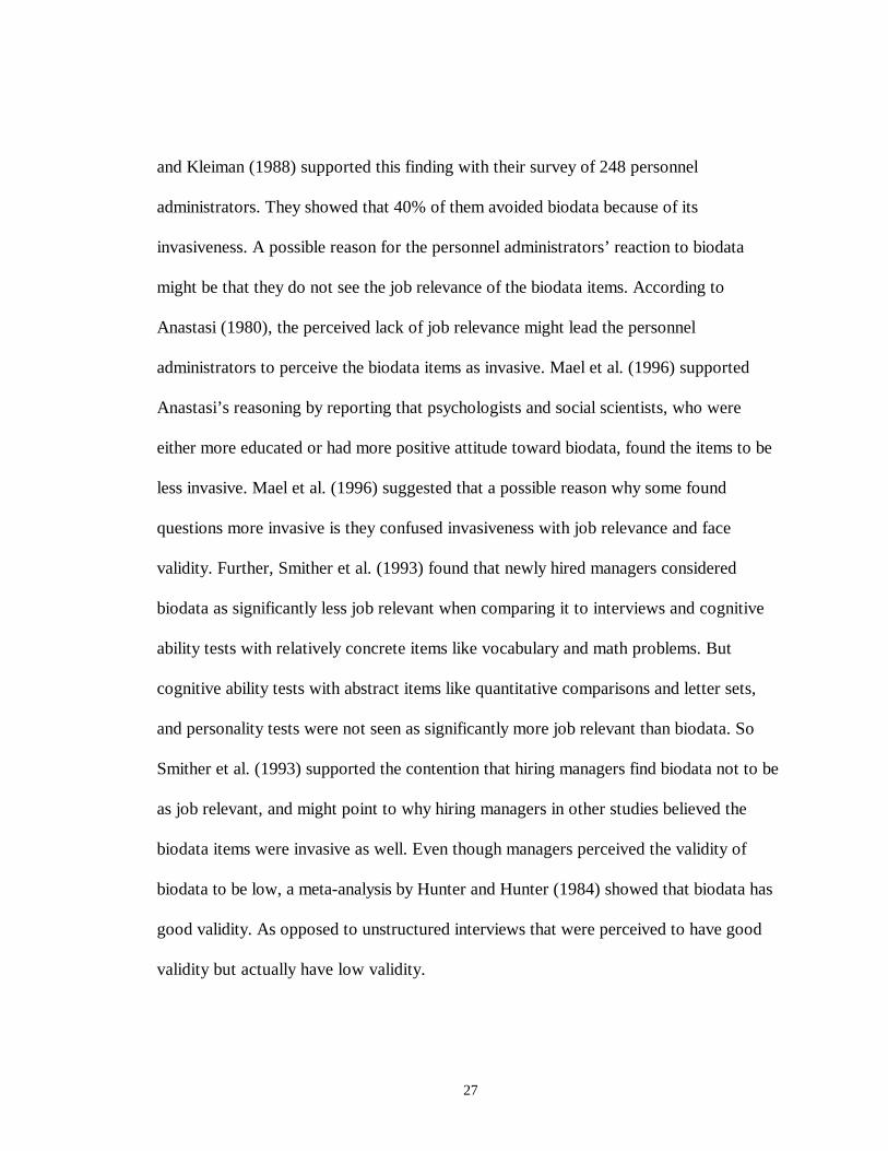
27
and Kleiman (1988) supported this finding with their survey of 248 personnel
administrators. They showed that 40% of them avoided biodata because of its
invasiveness. A possible reason for the personnel administrators’ reaction to biodata
might be that they do not see the job relevance of the biodata items. According to
Anastasi (1980), the perceived lack of job relevance might lead the personnel
administrators to perceive the biodata items as invasive. Mael et al. (1996) supported
Anastasi’s reasoning by reporting that psychologists and social scientists, who were
either more educated or had more positive attitude toward biodata, found the items to be
less invasive. Mael et al. (1996) suggested that a possible reason why some found
questions more invasive is they confused invasiveness with job relevance and face
validity. Further, Smither et al. (1993) found that newly hired managers considered
biodata as significantly less job relevant when comparing it to interviews and cognitive
ability tests with relatively concrete items like vocabulary and math problems. But
cognitive ability tests with abstract items like quantitative comparisons and letter sets,
and personality tests were not seen as significantly more job relevant than biodata. So
Smither et al. (1993) supported the contention that hiring managers find biodata not to be
as job relevant, and might point to why hiring managers in other studies believed the
biodata items were invasive as well. Even though managers perceived the validity of
biodata to be low, a meta-analysis by Hunter and Hunter (1984) showed that biodata has
good validity. As opposed to unstructured interviews that were perceived to have good
validity but actually have low validity.

28
Even though some psychologists, personnel administrators, and hiring managers
have concerns about the invasiveness of biodata items, limited research showed that
many applicants actually prefered biodata tests and saw them as fairer than other
selection tests. Research demonstrated that job incumbents prefered biodata selection
tests over general mental ability tests because they found them more fair and effective
(Mitchell, 1998). Minorities, women, and older applicants also perceived biodata to be
very fair (Mitchell, 1994). Kluger and Rothstein (1993) reported that applicants found
biodata to be more fair because they felt they had more control over getting the ‘right’ or
‘good’ answers and felt the test reflected better ‘who they are’.
Some of the attributes of biodata items are one of the reasons why some human
resource professionals and applicants perceive biodata as having low face validity, job
relevance, and invasiveness. Biodata items have five possible basic negative attributes
that can make them seem invasive or less job relevant, depending on the individual. The
first is verifiability or items with answers human resource professionals can verify. Some
researchers propose that verifiable items are invasive because applicants lose the power
to misrepresent themselves if they so choose to (Stone & Stone 1990). Others believe that
non-verifiable items will be more invasive because they ask about your own behaviors,
feelings, and thoughts (Mael et al., 1996). Controllability is another attribute that comes
into play with items that ask about life events a person may or may not have had control
over. Some research proposes that applicants will perceive items that ask about non-
controllable events as more invasive because applicants will find them unfair since they
have no control over the situation and the outcome (Mael et al, 1996). The negativity of

29
items, items that ask applicants about experiences that had negative consequences, is
another attribute that possibly makes biodata items seem invasive. Transparency is a
fourth attribute that might alter one’s perception of biodata items. Some human resource
professionals believe that items that are less transparent will be more invasive because
they will appear less job relevant. The final attribute, that might alter one’s perception of
biodata items, is how personal the item is. Items that ask more personal questions or non-
work related questions might be seen as more invasive (Mael et al., 1996).
Of these five attributes, Mael at al. (1996) found that applicants perceived biodata
that were more verifiable, more transparent, and less personal as less invasive. While
some researchers also believed that asking applicants about life events they had no
control over as invasive, Kluger and Rothstein (1993) found that applicants perceived
non-controllable items as less fair, but not more invasive than controllable biodata items.
Negative biodata items were not seen as invasive. A possible reason for this is that
applicants do expect organizations to ask them about past job failures or criminal
convictions. They consider the items to be job relevant questions (Mael et al., 1996).
Human resource professionals can take several steps can to minimize the
invasiveness of biodata items. First, avoid asking questions applicants will find too
personal. People tend to find questions about their religion, political affiliations, family or
spouse’s background, and sexual orientation or behavior to be invasive (Arnold, 1990;
Fletcher, 1992; Schuler, 1993; and Smart, 1968). So questions should stick to work,
school, or public related settings. Second step is to have better-written and verbal
descriptions that are given to applicants about the benefits, confidentiality, and purpose of

30
the selection procedure. Mael et al. (1996) showed that giving informative instruction to
individuals who have little knowledge of the concept of validity helped reduce the
perceived invasiveness of the biodata test. A final way to reduce invasiveness is to
increase the face validity of the selection test by using more transparent items. However
using more items where the ‘right’ or sociable correct answers are more obvious can
make faking or determining the ‘right’ answer easier for the applicants (Mael et al.,
1996).
Susceptibility to Faking
Research on the issue of fakability of biodata items shows mixed results.
Goldstein (1971) compared the answers of nursing applicants to information given to
their previous employers and found numerous discrepancies between them. Goldstein
(1971) demonstrated that applicants will lie on verifiable items, but human resource
professionals can check and catch the lying. Using college students, Doll (1971) assigned
subjects into one of three conditions: Doll (1971) instructed one group to (a) fake their
answers to look good, but to prepare themselves to defend their answers in an interview,
a second group to (b) fake the answers to look good, but to be aware that the test has a lie
scale to detect lying, lastly, a third group to (c) fake to look good as possible. The group,
that Doll (1971) just instructed to fake to look good as possible, lied the most. While the
group that he told a lie scale was present did the least amount of faking. Doll (1971) also
found that subjective items were more susceptible to faking than objective items. Becker
and Colquitt (1992) supported Doll’s (1971) finding by showing objective and verifiable
items were less susceptible to faking but furthered this by showing that applicants faked
31
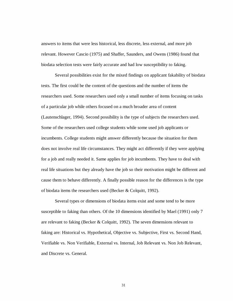
answers to items that were less historical, less discrete, less external, and more job
relevant. However Cascio (1975) and Shaffer, Saunders, and Owens (1986) found that
biodata selection tests were fairly accurate and had low susceptibility to faking.
Several possibilities exist for the mixed findings on applicant fakability of biodata
tests. The first could be the content of the questions and the number of items the
researchers used. Some researchers used only a small number of items focusing on tasks
of a particular job while others focused on a much broader area of content
(Lautenschlager, 1994). Second possibility is the type of subjects the researchers used.
Some of the researchers used college students while some used job applicants or
incumbents. College students might answer differently because the situation for them
does not involve real life circumstances. They might act differently if they were applying
for a job and really needed it. Same applies for job incumbents. They have to deal with
real life situations but they already have the job so their motivation might be different and
cause them to behave differently. A finally possible reason for the differences is the type
of biodata items the researchers used (Becker & Colquitt, 1992).
Several types or dimensions of biodata items exist and some tend to be more
susceptible to faking than others. Of the 10 dimensions identified by Mael (1991) only 7
are relevant to faking (Becker & Colquitt, 1992). The seven dimensions relevant to
faking are: Historical vs. Hypothetical, Objective vs. Subjective, First vs. Second Hand,
Verifiable vs. Non Verifiable, External vs. Internal, Job Relevant vs. Non Job Relevant,
and Discrete vs. General.

32
Although research showed that items that were more subjective, more
hypothetical, more job relevant and less verifiable were more susceptible to faking this
does not mean human resource professionals need to eliminate these types of items from
biodata selection instruments. One of the main benefits of biodata items is that applicants
find determining what is the ‘good’ or the ‘right’ choice very hard. So even though these
types are susceptible to faking it is difficult to fake well on a well-constructed biodata
test. In fact biodata is less susceptible to faking than personality tests (Allworth, 1999).
Also the most predictive items are usually the more subjective and less verifiable
answers. Verifiable answers tend to restrict the amount of information a biodata selection
test can obtain (Crafts, 1991). So having a balance of different types of items is
important.
Other steps besides limiting certain types of biodata items can reduce faking. The
first is using an empirical keying method over a rational scaling method. When using the
empirical keying method, applicants find figuring out the relationship between the items
and construct harder, as opposed to a rational scaling method where a more apparent
logical relationship exists. Hence, rationally developed items are more transparent, and
easier for applicants to figure out what answers are most “sociably desirable” (Haymaker,
1986 as cited in Becker & Colquitt, 1992; Kluger, Reilly, & Russell, 1991). A second
way to reduce faking is to construct a honesty scale and to warn applicants of the
presence of the honesty scale (Doll, 1971). A third way is to tell applicants, their answers
will be subject to verification and human resource professionals might ask them about
their answers in a follow up interview (Mumford & Owens, 1987).

33
Job Incumbents vs. Job Applicants
As mentioned earlier, the type of subjects used to construct the biodata test might
affect its validity. Many research studies use job incumbents to construct the biodata test
and then assume it will generalize to job applicants. But research alludes that the
potential job experience disparity and motivational differences between applicants and
incumbents might hinder the generalizability of the biodata test. Some researchers believe
that because job incumbents have more job experience, they will respond differently than
applicants to some items, and therefore the selection test will not generalize to the
applicants. A hypothesis concerning this states that job incumbents’ job experience may
influence the validity of concurrently derived keys (Hogan, 1994). Therefore if job
experience does affect concurrent validity, then concurrent validities should generally be
greater than predictive validities (Rothstein et al, 1990). In examining over 100 validity
studies, Hough (1986) found the median concurrent validities for those studies exceeded
the predictive validity for those studies for the following criteria: ranking, rating,
production, absenteeism, turnover, tenure, and delinquency (as cited in Hogan, 1994).
Thus, the higher median concurrent validity may mean that job experience was increasing
the validities for job incumbents and hence made a difference. Hogan (1988) supported
Hough’s research with similar findings. However, Rothstein et al. (1990) meta-analysis
demonstrated that job experience did not increase validities. Therefore, job experience
between incumbents and applicants might not matter when it comes down to
generalizability. Instead, Rothstein et al. (1990) suggested that motivational differences
as the possible reason for the disparity between the concurrent and predictive validities.

34
Job incumbent constructed selection tests might not generalize to applicants
because applicants will respond in a more sociably desirable way. Two types of socially
desirable responding exist. One is self-deception where people have unconscious
tendency to see themselves in a positive light. Second is impression management where
people consciously attempt to present themselves in a positive way (Stokes & Hogan,
1993). Stokes and Hogan (1993) suggested that when responding to a selection test,
applicants and incumbents commit similar amounts of unconscious self-deception, but
applicants usually perpetrate more impression management responding because they
want to increase their chances of getting a job. Stokes and Hogan (1993) used the index
of Socially Desirable Responding (SDR) to measure the amount of impression
management responding that was done in incumbent and applicant constructed biodata
keys. They demonstrated that the applicant and incumbent biodata keys did not match up.
They found that socially desirable responding could account for as much as 25% of the
variance between the two keys. They found that impression management was most
prevalent in items asking about preferences and self-evaluation of abilities, while
impression management was least likely in items relating to previous work or objective
and verifiable items.
Human resource professionals can minimize the possible effects of social
desirable responding and job experience on the biodata test. Human resource
professionals can minimize social desirability responding by simply taking the same steps
as mentioned earlier, when talking about reducing fakability of items. And asking
incumbents to respond only with experiences they obtained prior to their current job or by

35
rewording items so that they only ask about situations in previous job experiences can
reduce the effects of job experience (Stokes & Hogan, 1993).
Dust Bowl Empiricism
A final concern or reason some human resource professionals do not use biodata
is that they criticize the empirical approach of developing biodata keys as being “dust
bowl” or “blind” empiricism. Researchers agree that empirical approach has strong
predictor ability, but they also agree that it does little to explain the relationship between
the item and the criterion prediction and, hence the method relies to heavily on statistical
chance. Therefore, the method does not help in further development of any constructs or
theories (Dunnette, 1962). However, Drakeley (1988) believed that if the practitioner is
willing to investigate and do research a logical explanation could be discovered to
explain the relationship between the item and construct (as cited in Harvey-Cook, 2000).
Human resource professionals also have concerns about defending these empirical
findings logically in court. Just being able to show empirical evidence of biodata’s
predictive power might not be enough anymore. Human resource professionals might
need logical explanations of how the item relates to the construct. However, a benefit of
biodata, that might help reduce legal ramifications, is minorities, women, and older
people (protected groups) find biodata to be very fair (Mitchell, 1994). Even though the
protected groups perceive it, as being very fair, human resource professionals still need to
prepare to defend the items they use empirically and logically.
The following are two sample questions that demonstrate how the empirical
method can provide predictive power and explanation without providing little if any

36
logical explanation. The question “Did you ever build a model airplane that flew” was an
excellent predictor of flight training success in World War II (Cureton, 1965). Logically,
one might reason that people who build model airplanes take great interest in how planes
work and how one designs a plane. Therefore they have a better understanding of planes
when entering flight training school and as a result do better. A second example that
provides evidence for “dust bowl” empiricism at work is the predictive relationship
between attendance at a circus show and success at being a door- to-door salesman
(Appel & Feinberg, 1969).
Summary
Even though biodata has some negative perceptions, as do all selection measures
do, it proves to be valid in the selection process. Biodata helps organizations select the
right people for the right job by systematically measuring a person’s past behavior
through empirical, rational, or factorial scaling methods to indirectly measure the
person’s future behavior and performance. When constructed properly, biodata can have
good predictive validity, low adverse impact, low susceptibility to faking, and low
invasiveness. Human resource professionals can also design biodata to be
organizationally specific to increase the predictive validity, or design it to generalize
across organizations and jobs. Research shows that biodata is a valuable asset to the
selection process, especially when human resource professionals use it in conjunction
with GMA, personality measures, or interviews. Biodata is an inexpensive selection
measure that gathers a broad range of information and predicts several criteria for job
success.

37
CHAPTER 2
BIODATA STUDY
Rationale for Using Biodata and the Hypotheses of the Study
Because the current increase in technology leads to increasing global competition,
companies look for more ways to communicate to more customers their products, ways to
get the product to their customers faster, and ways to help the customer shop from the
privacy of their own home. One way companies do this is through the use of catalogs and
the Internet. More companies today rely on call centers to help sell their product (William
Olsten Center, 1998). As a result, many catalog customer service representatives (CSR’s)
make the important initial contact with potential customers for the company. So ideally
companies want experienced and well trained CSR’s talking to potential customers to
make the experience as enjoyable as possible for the customer.
However, many call centers experience a very high turnover rate. The William
Olsten Center For Workforce Strategies survey of 424 call centers throughout the U.S.
and Canada and found that, on average, call centers only retain 1 out of every 3
employees they hire (William Olsten Center, 1998). In fact, turnover rates over 100% are
not uncommon for some call centers (Levin, 2000). Surveys show the larger the call
center, the higher the turnover rate. As a result of the high turnover, call centers
experience high financial and organizational costs for the hiring and training of CSR’s
(William Olsten Center, 1998).
38
Many companies also admit their turnover rate is getting worse and is not likely to
improve, so they do not actually try to improve on it (“Hallis Release”, 1999; Levin,
2000; Thomas Staffing, 1999). One problem the companies might have is with their
selection process. Ninety-four percent of companies said they use the interview process
to identify characteristics of a good call center employee, to identify applicant’s with a
“positive attitude” and “strong work ethic” (William Olsten Center, 1998).
Characteristics like these can be hard to identify in the interview process, especially if the
human resource professionals do not structure the interview correctly to measure them.
One possible way to improve on retention and identify employees who will stay
longer is through the use of biodata. Biodata is an ideal tool to help in the selection
process to identify retention in CSR’s. Biodata has good predictive validity for tenure
(Hogan, 1994). And biodata is most useful for jobs that have repetitive actions like CSR’s
have (Mitchell, 1994). Human resource professionals can also use biodata as a
prescreening tool to the interview. This will cut down on time and potentially cut down
on training costs if the process selects the right people.
Developing a biodata selection instrument to improve the retention rate of CSR’s
in a major U.S. retail company was the purpose of this study. Biodata items, developed
by an outside consultant to predict turnover, were used to see if they generalize and hence
predict the retention rates of the CSR’s. The biodata items, constructed from an
accumulation of previous research done by the outside consultant, were not job specific.
Previous research shows that generalizable biodata items focus on core criterion
measures or attributes that focus on many jobs and that are not job specific or situation

39
specific. Rothstein et al. (1990) and Carlson et al. (1999) demonstrated this by not
focusing on functional specialties in their studies. Several studies showed that biodata
tests have a mean predictive validity of r = .30-.40 for numerous criteria including tenure
(Hunter & Hunter, 1984; Reilly & Chao, 1982; Schmitt, et al., 1984). Since the biodata
items were not situation specific and biodata has good mean predictive validity for
tenure, the biodata items were expected to generalize and be predictive of retention for
CSR’s.
Hypothesis 1: The biodata items will be predictive of retention in CSR’s. The
biodata items will differentiate between the high and low retention groups for all scoring
methods.
Cross-validation is used to determine what biodata items will predict retention.
The steps of cross-validation were first to divide the study’s sample into two groups, a
development group and a holdout group. Second, the development group was used to
score and weight the biodata items. Next, these weights were applied to the holdout group
to predict their retention. Then the holdout member’s scores were compared to their
actual retention rates to make sure the weights for the biodata items did not simply occur
by chance.
Five different empirical methods were used to score and weight the items. The
empirical methods were the Mean Standardized Criterion Method (MSC), Option
Criterion Correlation Method (OCC), Horizontal Percentage Method (HPM), Vertical
Percentage Method (VPM), and Weighted Application Blank Method (WAB). The
Method section describes these methods in detail. The little reported research on these

40
methods showed that when comparing the HPM and VPM methods that they correlated
in the high .90’s. Research also showed that the OCC method correlated r = .93 with
VPM and r = .94 with the MSC method. The VPM also correlated well with the MSC
method (r. = .78) (Mitchell, 1994). The VPM approach is also conceptually similar to the
OCC method, as is the HPM approach to the MSC method. Both the VPM and OCC
method are similar because each option gets a positive or negative weighted value
depending how the option relates with the high and low criterion groups. The HPM and
MSC method relate conceptually because each option’s weight depends on the item
response’s direct relation to how successfully it predicts the criterion (Mitchell, 1994).
England’s (1971) WAB method has little or no reported research comparing it with these
other methods. England’s (1971) WAB method is similar to the VPM method, but
England (1971) recommends one further step: to convert the VPM weights (which are
determined by looking at Strong’s Net Weights) to his Assigned Weights. England
(1971) recommends this to eliminate negative weights and to eliminate any differences
that might have occurred by chance or error between the high and low criterion groups.
So the scoring methods are looked at to see if they identify the same amount of
people for the high and low retention groups. Since the first four methods either
correlated high with one another or are conceptually similar, the first four methods were
expected to identify similar amounts of people in each criterion group. England’s (1971)
WAB method was not expected to predict the same amount of people in each criterion
group because of England’s (1971) recommendation. England’s (1971) recommendation
safeguards against any possible differences that might occur by chance from using a

41
small sample size, but a large sample size is used in this study and therefore the Assigned
Weights may minimize differences or over correct errors that might occur by chance.
And therefore eliminate some of the predictive items that the other approaches might use
to differentiate between the high and low criterion groups and hence hurt how well the
WAB method would discriminate between high and low criterion groups.
Hypothesis 2a: The VPM, HPM, OCC, and MSC approaches will similarly
discriminate between the high and low criterion groups.
Hypothesis 2b: The WAB method, with England’s recommendation to use
Assigned Weights, will not discriminate as well between the high and low criterion
groups as the other four methods.
All the scoring methods were checked to see if adverse impact occurred.
Numerous studies showed that biodata creates little or no adverse impact with proper
construction (Mitchell, 2000; Reilly & Chao, 1982; Rothstein et al., 1990; Wilkinson,
1997). Several steps were taken to ensure proper construction. First, the biodata items,
used, were developed from previous research by an outside consultant to specifically
predict turnover. Second, applicants could answer all the biodata items because item
responses like ‘not relevant’ were included when needed. Third, any items that created
adverse impact had their item scoring weights set to zero to eliminate their effects on the
selection measure. Therefore the biodata selection test should produce little or no adverse
impact.
Hypothesis 3: The biodata selection test under each scoring method will have
little or no adverse impact with proper construction.

42
The company’s goal was to use biodata to increase the retention rate as far above
the mean retention rate, M = 3.6 months, as possible so that the company could better
cover the time and costs of hiring and training the new employees. Ideally, the company
wanted to get the retention rate above 6 months because employees who work for 6
months or less are more likely to leave the company. After 6 months, companies want to
hire people who will stay a year to 2 years because at that point, employees are even
more likely to stay (Thomas Staffing, 1999). However that is rare in the call center
industry; usually one to two years is the max anyone will stay before moving onto a
different line of work (William Olsten Center, 1998). At this company raising the
retention rate this high was not an option since the company reported the average
retention rate to be at or near 3 months and the company did not have enough CSR
employees with retention rates longer than a year to identify characteristics that
distinguish employees who stay longer than a year to employees that do not.
Method
Participants
The original sample consisted of 1515 currently employed or previously
employed customer service representatives (CSR’s) from over 15 different catalog call
centers from across the U.S. for a major U.S. retail company. The original sample had a
mean retention rate of 3.60 months and SD = 2.48. The sample consisted of 1205 females
and 310 males. The sample also consisted of 833 Whites, 534 Blacks, 119 Hispanics, 19
Asian/Pacific Islanders, and 10 American Indians/Alaskans.

43
The original sample was then divided into a development group and a holdout
group for future cross-validation purposes. The development group consisted of 865
CSR’s and the holdout group consisted of 434 CSR’s. The development sample had 694
females and 171 males. The sample also consisted of 475 Whites, 305 Blacks, 67
Hispanics, 12 Asian/ Pacific Islanders, and 6 American Indian/Alaskans. The holdout
group consisted of 434 CSR’s. The group had 351 females and 83 males. The sample also
consisted of 234 Whites, 156 Blacks, 34 Hispanics, 7 Asian/Pacific Islanders, and 3
American Indian/ Alaskans.
Procedure
Over 250 biodata items, developed by an outside consultant to predict turnover in
jobs, were reviewed. With help from the human resource consultant at the retail
company, and a job description of what the CSR’s do, the number of items were reduced
to 63. The items believed to best identify retention in CSR’s, based on the knowledge,
skills, and abilities needed for the job, were chosen. Any items asking about job
experience were then rewritten so that they asked CSR’s to respond with only job
experiences they had prior to this job. This was done to help minimize any effects job
experience might have on their responses.
A cover letter was then sent to all the managers of the 15 call center locations
throughout the U.S. to explain the purpose and development of the biodata selection
instrument. An overview of the project was also sent for the CSR’s. The overview
explained the purpose of the survey (to create a selection test) and that their participation
was voluntary. The overview assured them that their answers would remain confidential

44
and would not affect their job status or compensation. The overview also explained how
long the survey would take to answer. Once completed, the call centers sent the surveys
back, and the data was entered into PC-File and then transferred into SPSS for analysis.
To determine which items were predictive of retention, a cross-validation strategy
was used. First, the company measured retention by the employees’ time in the company.
After determining how to measure the criterion, the decision on how to divide the sample
into the high and low criterion groups was determined. The goal was to raise the mean
retention rate above 3.6 months and ideally to 6 months. But because setting the high
criterion group at 6 months would create too small of a group, the high criterion group
was set at employees who stayed 5 months or longer. England (1971) recommended that
each group have at least 150 employees, some recommended at least 500, and Nunnally
(1978) recommended that a ratio of 5 to 10 people be used for every biodata question
used (Brown, 1994). Setting the high criterion group at 6 months would have put the
group under 150 people and the sample size would not have been sufficient for validation
purposes. The low criterion group was set at 3 months and under. Next, any employees
who had retention rates between 3 and 5 months were excluded from the study. Also any
employee under 3 months who was still currently employed was excluded because it
could not be determined how long the employee would eventually stay. Hence leaving
them in the low criterion group would contaminate this criterion group, if those
employees ended up staying longer than 3 months.
The original sample was divided into a development group and a holdout group,
for cross validation purposes. Cross-validation strategy was chosen because of time

45
constraints. England (1971) recommends using a 2 to 1 ratio between the development
and holdout group. The development group contained 865 CSR’s and the holdout group
contained 434 CSR’s. The employees were divided into the development and holdout
group so that their percentages in the development and holdout group for number of
people from each location, race, and gender matched as close as possible the percentages
for the total sample for location, race, and gender.
After creating the items and groups, and entering and analyzing their responses,
five different empirical scoring methods were used to determine the item weights. The
Mean Standardized Criterion (MSC) Method was used first. The initial step was to
calculate the mean for each response option for all 63 items. Next, setting the mean for
each item to 0 and standard deviation to 1 standardized the criterion variable. Then the
criterion means for each option scoring response were multiplied by ten and rounded to
the nearest whole number to determine the option response’s scoring weight.
The Option Criterion Correlation (OCC) was the second method. The initial step,
here, was to correlate each option response with the continuous criterion variable or time
in company (retention). Then the correlation was set up so that a correlation of or near 1
means the response item endorsed high retention, correlation of or near –1 means the
response item endorsed low retention, and a correlation near zero did not indicate a
predictive retention response. Lastly, the correlation was multiplied by 100 and rounded
to the nearest whole number to determine the scoring weight.
The Horizontal Percentage Method (HPM) was the third method. First step in this
method was, for each item, determining the total percentage of people from the high

46
criterion group who responded to each option response. Then the percentage was divided
by the total percentage of people who choose that option regardless of whether they were
in the high or low criterion group. Next, the quotient was multiplied by 10 to determine
the scoring weights for the response options.
The Vertical Percentage Method (VPM) was the fourth method. To determine the
scoring weights, for each item, the total percentage of people from the high criterion
group who respond to each option response was calculated. Then the step was repeated
using the low criterion group. Next, for each response option the percentage of low
criterion group who responded was subtracted from the percentage of the high criterion
group who responded to that particular option. Lastly, Strong’s Net Weights are used to
convert these percentage differences into scoring weights (England, 1971).
England’s (1971) Weighted Application (WAB) Method was the final method.
This method is similar to the VPM method but takes one further step. After using
Strong’s Table to determine the response option weights, England (1971) recommends
converting Strong’s Net weights to Assigned Weights from his table. His table simplifies
the scoring by making all the weights positive instead of having negative and positive
weights, which researchers might confuse in future applications. England (1971) also
suggests using the table to eliminate or correct for any differences that might occur by
chance or error between the high and low criterion groups.
After determining the scoring weights, the weights were applied to the holdout
group to see if they predicted retention in that group. The overall selection rates of the
five methods were then tested for adverse impact by using the Four-Fifth’s Rule. Four-

47
Fifth’s Rule states that selection ratio of any group must be at least 80 percent of the
selection ratio of the most favorably treated group. Specifically, adverse impact against
race and gender was checked. To compare the scoring methods, the cutoff score for each
method was set so that it eliminated 40% or close to it of the low criterion group. Forty
percent was chosen to eliminate most of the low criterion group and also at the same time
to retain around ¾ of the high criterion group or more. After determining the cutoff score,
the scoring methods were compared by looking at the amount of adverse impact each
created, the scoring method’s hit-miss ratio on the high criterion group (since low
criterion group will be at or near 40% for all the methods), and how well the scoring
method increased the retention rate. How well the methods correlated with each other and
the criterion measure was also looked at.
After comparing the scoring methods on the aforementioned criteria, the scoring
weights for each item were then checked to see if they created any adverse impact and if
so they were set to zero for those items. After eliminating the effects of any adverse
impact items, the aforementioned comparisons were again looked at to see how well the
scoring methods compared once adverse impact items were eliminated.
Results
Hypotheses for this study are:
Hypothesis 1: The biodata items will generalize or be predictive of retention in
CSR’s. The biodata items will differentiate between the high and low retention groups for
all scoring methods.

48
Hypothesis 2a: The VPM, HPM, OCC, and MSC approaches will similarly
discriminate between the high and low criterion groups.
Hypothesis 2b: The WAB method, with England’s recommendation to use
Assigned Weights, will not discriminate as well between the high and low criterion
groups as the other four methods.
Hypothesis 3: The biodata selection test under each scoring method will have
little or no adverse impact with proper construction.
To test these hypotheses, several steps were taken. First, the five scoring methods
were used to determine the scoring weights for each item response using the development
group. Appendix A presents the scoring weights for each item response by each method.
All the scoring methods except the WAB method produced different weights for each
item response. The WAB method gave a scoring weight of one for all the item responses
and therefore did not discriminate between high and low criterion groups. This did not
support the first hypothesis, in that one of the scoring methods did not predict retention.
As a result, no further analysis on the WAB method was done for adverse impact and
criterion prediction, since every applicant would receive the same score.
After computing and running the frequencies of the applicants’ total scores (sum
of the scoring weights on all 63 items) for both the high and low criterion groups in the
holdout sample, the cutoff score was set by choosing the score closest to the one that
eliminated 40% of the low criterion group. The cutoff scores for OCC, MSC, HPM, and
VPM were -10, -13, 312, and –2, respectively. The cutoff scores eliminated 20.3%,
18.2%, 25.1 %, 20.9% of the high criterion group for the OCC, MSC, HPM, & VPM,

49
respectively. The four/fifths rule was then used to test each of the four scoring methods’
overall selection rates for racial and gender adverse impact. Since the sample contained
only large percentages of Blacks and Whites and not a big enough percentage of any
other ethnic group, those two races were looked at when determining if racial adverse
impact existed. Table 3 shows the gender and race selection rates for each of the four
methods. Table 3 shows the four methods do not fail the four/fifths rule for gender but all
of them do for race, indicating the four methods show adverse impact against Blacks.
Appendix B shows that even when comparing the selection rates of Whites and all Non-
Whites in the sample that the percentages of other minority races in the sample were so
small that they do not change the outcome of the four//fifths rule for racial adverse
impact. The scoring methods still show racial adverse impact.
Table 3.
Gender and Race Selection Percentage Rates of the Holdout Sample for each of the Four
Scoring Methods
Gender Race
Scoring Methods Male
n = 83
Female
n = 351
AI Ratio Black
n = 156
White
n = 234
AI Ratio
OCC .69 .69 1.0 .50 .82 .61
MSC .69 .71 .97 .55 .81 .68
HPM .67 .79 .85 .58 .83 .70

50
VPM .71 .72 .99 .57 .82 .70
Note. Selection rates are rounded to nearest whole percent. AI Ratio = Adverse impact
ratio. The lower selection rate is divided by the larger selection rate to determine the AI
Ratio. AI Ratio ? .80 means no adverse impact.
To test the hypothesis that the scoring methods are different from each other, the
ability of each method to predict success or discriminate between the high and low
criterion groups below and above the cutoff score in the holdout sample was investigated.
The mean retention rates for the high and low criterion groups above and below the
cutoff score were calculated to determine how well the scoring methods discriminated
and improved retention. Table 4 shows the mean retention rates for each group and shows
the results of an independent t- test used to compare the means of the two criterion
groups.
Table 4.
Comparison of Mean Retention Rates of the Holdout Criterion Groups for each of the
Four Scoring Methods
Scoring Method High M High SD Low M Low SD t
OCC 4.1 2.6 3.0 2.3 4.42**
MSC 4.1 2.6 2.8 2.3 5.18**
HPM 4.0 2.6 3.0 2.4 3.95**
VPM 4.1 2.6 2.8 2.3 4.93**
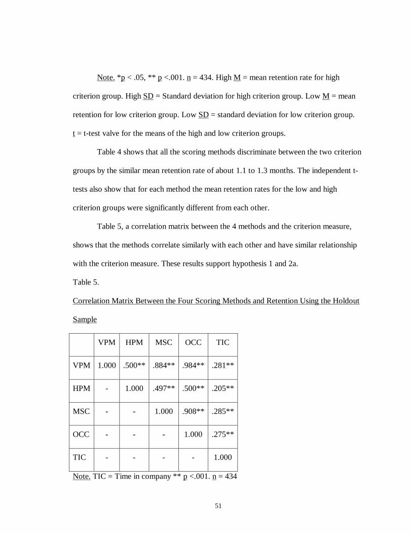
51
Note. *p < .05, ** p <.001. n = 434. High M = mean retention rate for high
criterion group. High SD = Standard deviation for high criterion group. Low M = mean
retention for low criterion group. Low SD = standard deviation for low criterion group.
t = t-test valve for the means of the high and low criterion groups.
Table 4 shows that all the scoring methods discriminate between the two criterion
groups by the similar mean retention rate of about 1.1 to 1.3 months. The independent t-
tests also show that for each method the mean retention rates for the low and high
criterion groups were significantly different from each other.
Table 5, a correlation matrix between the 4 methods and the criterion measure,
shows that the methods correlate similarly with each other and have similar relationship
with the criterion measure. These results support hypothesis 1 and 2a.
Table 5.
Correlation Matrix Between the Four Scoring Methods and Retention Using the Holdout
Sample
VPM HPM MSC OCC TIC
VPM 1.000 .500** .884** .984** .281**
HPM - 1.000 .497** .500** .205**
MSC - - 1.000 .908** .285**
OCC - - - 1.000 .275**
TIC - - - - 1.000
Note. TIC = Time in company ** p <.001. n = 434

52
To help eliminate the adverse impact, each of the 63 items were checked for racial
adverse impact for the four methods. To determine if adverse impact existed, the scoring
weights were applied to the holdout group and the mean scores for Blacks and Whites for
each item for all four methods were compared. To reduce adverse impact as much as
possible, the scoring weights of any items that were significantly different at the .10 level
were eliminated (see Appendix C) by setting them to zero. This way the item will not
affect the outcome of the biodata measure. This process eliminated several items’ weights
for each scoring method indicating that some of the items did create adverse impact. The
process eliminated the scoring weights for 25, 21, 16 and 26 items from the OCC, MSC,
HPM, and VPM, respectively. For all four scoring methods, the process only eliminated
12 items that were the same. Once the item weights were set to zero, each applicant’s
total score was adjusted accordingly. Next, the steps mentioned earlier were repeated to
determine the cutoff scores. The new cutoff scores for OCC, MSC, HPM, and VPM were
2, -8, 233, and 1, respectively. The cutoff scores eliminated 25.7%, 23.5%, 16.6 %,
21.4% of the high criterion group for the OCC, MSC, HPM, & VPM, respectively.
After determining the cut off scores, the four/fifths rule was used again to test
each of the four scoring methods’ overall selection rates for racial and gender adverse
impact. Table 6 shows the gender and race selection rates for each of the four methods
after the adverse items were set to zero. Table 6 shows that after checking for and
eliminating the effects of the adverse impact items, none of the methods fail the
fourth/fifths rule for race or gender. These results support the third hypothesis that with
proper construction biodata can create little or no adverse impact.

53
Table 6.
Gender and Race Selection Percentage Rates of the Holdout Sample for each of the Four
Scoring Methods After Eliminating Adverse Impact Items
Gender Race
Scoring Methods Male
n = 83
Female
n = 351
AI Ratio Black
n = 156
White
n = 234
AI Ratio
OCC .70 .66 .94 .59 .72 .82
MSC .65 .68 .96 .60 .72 .83
HPM .70 .79 .89 .71 .82 .87
VPM .73 .70 .96 .62 .76 .82
Note. Selection rates are rounded to nearest whole percent. AI Ratio = Adverse impact
ratio. The lower selection rate is divided by the larger selection rate to determine the AI
Ratio. AI Ratio ? .80 means no adverse impact.
To once again test the hypothesis that the scoring methods are different from each
other, the ability of each method to predict success or discriminate between the high and
low criterion groups below and above the cutoff score in the holdout sample was
investigated. The mean retention rates for the high and low criterion groups above and
below the cutoff score were calculated to determine how well the scoring methods
discriminated and improved retention. Table 7 shows the mean retention rates for each

54
group and shows the results of an independent t- test used to compare the means of the
two criterion groups.
Table 7.
Comparison of Mean Retention Rates of the Holdout Criterion Groups for each of the
Four Scoring Methods
Scoring Method High M High SD Low M Low SD t
OCC 4.0 2.6 3.2 2.4 3.26**
MSC 4.0 2.6 3.3 2.5 3.11*
HPM 3.9 2.6 3.2 2.5 2.51*
VPM 3.9 2.6 3.1 2.4 3.28**
Note. *p < .05, ** p <.001. n = 434. High M = mean retention rate for high
criterion group. High SD = Standard deviation for high criterion group. Low M = mean
retention for low criterion group. Low SD = standard deviation for low criterion group.
t = t-test valve for the means of the high and low criterion groups.
Table 7 shows that all the scoring methods discriminate between the two criterion
groups by the similar mean retention rate of about .7 to .8 months. The independent t-
tests also show that for each method the mean retention rates for the low and high
criterion groups were significantly different from each other.
Table 8, a correlation matrix between the 4 methods and the criterion measure,
shows that the methods correlate similarly with each other and have similar relationship
with the criterion measure. These results also support hypothesis 1 and 2a.

55
Table 8.
Correlation Matrix Between the Four Scoring Methods and Retention Using the Holdout
Sample After Eliminating the Adverse Impact Items
VPM HPM MSC OCC TIC
VPM 1.000 .406** .664** .892** .156**
HPM - 1.000 .445** .402** .144**
MSC - - 1.000 .763** .181**
OCC - - - 1.000 .174**
TIC - - - - 1.000
Note. TIC = Time in company ** p <.001. n = 434
Discussion
The research shows that four out of the five methods are useful in increasing the
retention rate of the CSR’s. The methods do not increase the retention rates as much as
the company would have liked. One possible reason for this is that the biodata questions
are not organization-specific or job specific. Research shows that job specific or
organization specific biodata items will be more predictive but less generalizable to other
jobs. Another possible reason limiting the effectiveness of the biodata is the lack of
difference in tenure between the high and low criterion groups. To increase the retention
rate more, biodata needs a bigger difference between the low and high criterion group.
But because retention in the company is so low to begin with, the sample lacks the
necessary numbers to set the high criterion group at a retention rate above 5 months.

56
The WAB method does not show any items will be predictive of retention. All the
items received the same weight. One possible reason for this is England’s (1971)
adjustments safeguard against chance errors that might occur in samples, specifically
smaller samples that are not truly representative of the population. But this study has a
large sample size (Hogan, 1994) and therefore England’s (1971) adjustment scale might
over correct for chance errors or eliminate differences that are actually representative of
the population and that do not occur by chance.
The research does however support previous studies by showing that biodata
selection instruments with proper construction create little or no adverse impact for race
and gender. But the study also shows that the predictive validity of the four scoring
methods decreases when attempting to reduce the adverse impact of the selection
measure. The OCC method goes from r = .275 to r = .174, the MSC goes from r = .285 to
r = .181, the HPM goes from r = .205 to .144, and VPM goes from r = .281 to r = .156.
Consequently, the difference between the mean retention rates of the low and high
criterion groups also decreased. So to obtain and adverse impact free test, the company
must be willing to lose some of the test’s predictive ability. However, since the biodata
selection test does correlate significantly with retention, the company does not have to
eliminate the adverse impact items if the company can prove that having the retention
rate that high is a business necessity and no other valid test with less adverse impact is
available.
The research also shows that one must not just assume biodata questions are free
of adverse impact. In fact, depending on the scoring method used some items might cause

57
adverse impact and some might not. In this study the item adverse impact analysis
eliminates the least amount of items from HPM method and hence the HPM method has
higher selection rates for both race and gender.
Lastly, these results support limited previous research that shows the VPM, HPM,
OCC, and MSC methods are similar. When comparing the methods to each other, no one
method seems to greatly improve the retention rate or greatly reduce adverse impact over
the others. So no one method appears to be more beneficial, but as mentioned earlier,
they are not interchangeable without checking for adverse impact first.
Limitations of the Study
The study has some possible limitations that might affect its results. The first is
the criterion measure the biodata test uses. A biodata test is only as good and reliable as
its criterion measure. The criterion measure in this study is the employee’s time in the
company. Biodata uses this criterion measure to differentiate between employees who
leave the company before 3 months and those who stay longer than 5 months. The
company does not want to waste money on hiring and training employees who will stay
less than 3 months. However the criterion measure does not tell whether the employees
who leave before 3 months leave because of promotion within the company or leave the
company voluntarily or involuntarily. So valuable employees who the company promotes
before 3 months (if this does occur), were included with the low criterion group. As a
result, this somewhat distorts the item response weights of the low criterion group. Also
the high criterion group includes employees still currently with the company. Therefore,
these employees’ retention measures, at the time of this study, are an underestimate of

58
their actual employee tenure with the company. Hence, the biodata results might
underestimate the differentiation between the high and low criterion groups.
Another factor concerning the criterion measure is the objectiveness of it. One
possibility that might affect the objectiveness of the criterion is the call center managers’
biases. If managers fire good workers for personal reasons and not job related reasons,
these biases will affect the objectivity of the criterion measure.
Another possible limitation that will affect the generalizability of the selection test
to applicants is the job incumbents used to develop the test. Research shows that social
desirability and job experience might hinder the generalizability of the results to
applicants. Steps were taken to minimize job experience by rephrasing questions so that
they ask about previous job experiences. But the job incumbents’ motivation to take the
test might alter their responses and hinder the generalizability of the test.
Future Research and Recommendations
Overall, organizations need to make sure if they use ‘generalizable’ biodata tests
and not ones that they create specifically for themselves, that they first test the validity of
the biodata instrument and second make sure they have a strong criterion measure and
representative sample group. The organization must also reevaluate the validity of the
instrument at least every 2 years. Finally, as this study shows, the organization cannot
assume that generalizable biodata items are also adverse impact free. This study shows
that human resource professionals still need to check items for adverse impact, especially
if the organization changes scoring methods to reweight the item responses.

59
Organizations must also remember the biodata selection test can be very useful in
enhancing the hiring process. But like all methods, biodata is just one tool that can help
and organizations should not use it as the sole tool in the decision making process. No
one tool exists that can find the perfect applicant 100% of the time, but biodata is a cost-
effective tool that can help increase the odds of finding that good quality employee.
Lastly, this research shows that the biodata test will only be as good as its
construction. The sample and lack of range in the criterion variable limits the predictive
ability of the biodata test. So organizations must consider carefully if they have the
sample and the criterion measure available to get the desired results they want before
implementing a biodata selection measure.
Further research in biodata needs to be done on using job incumbents vs. job
applicants to create a scoring key. Specifically, future research needs to look at the job
environment and job attitudes of the job incumbents. Usually companies implement new
hiring measures because retention is poor. If this is the case, and turnover is high, morale
might be a problem in the workforce because people are losing friends or cannot bond
with new coworkers before they end up leaving. This can create a poor work environment
and hence affect the attitude of the job incumbents when they take the test. If they do not
believe the test will work then they might not take it seriously and just fill out the test as
fast they can to get it over with. But job incumbents, who work in a healthy job
environment and believe that this new biodata test is important to bettering the work of
the company, might take the test more seriously and answer the questions differently.
With downsizing becoming a norm practice for many companies, this might be an

60
important issue to look at when developing not only future biodata tests, but any selection
test.

61
APPENDIX A
SCORING WEIGHTS FOR EACH ITEM RESPONSE UNDER THE FIVE SCORING
METHODS

62
SCORING WEIGHTS FOR EACH ITEM RESPONSE UNDER THE FIVE SCORING
METHODS
Item #
Q1 M SD n n high
n low
% high
% low
MC OC HM VM WB
1 A 3.25 2.74 78 32 46 8.6 9.3 -2 -1 5 0 1 2 B 3.61 2.70 197 89 108 23.9 22.0 1 2 5 0 1 3 C 3.71 2.76 334 155 179 41.7 36.4 2 5 5 1 1 4 D 3.14 2.62 247 94 153 25.3 31.1 -3 -6 4 -1 1 5 E 2.33 2.05 8 2 6 0.5 1.2 -11 -4 3 -1 1 Total 3.47 2.71 864 372 492 100 100
Q2 M SD n n high
n low
% high
% low
MC OC HM VM WB
1 A 3.33 2.61 248 100 148 26.9 30.0 -1 -3 5 -1 1 2 B 3.42 2.71 409 170 239 45.7 48.5 -1 -3 5 -1 1 3 C 3.71 2.81 205 100 105 26.9 21.3 2 7 6 1 1 4 D 5.28 2.44 3 2 1 0.5 0.2 18 3 7 0 1 Total 3.47 2.71 865 372 493 100 100
Q3 M SD n n high
n low
% high
% low
MC OC HM VM WB
1 A 3.47 2.85 110 47 63 12.7 12.8 0 0 5 0 1 2 B 2.72 2.62 109 35 74 9.5 15.1 -7 -8 4 -1 1 3 C 3.62 2.70 91 40 51 10.8 10.4 1 1 5 0 1 4 D 3.79 2.66 188 94 94 25.4 19.1 3 7 6 1 1 5 E 3.47 2.69 267 112 155 30.3 31.6 0 -1 5 0 1 6 F 4.56 3.31 14 8 6 2.2 1.2 11 4 6 1 1 7 G 3.35 2.57 82 34 47 9.2 9.6 -1 -1 5 0 1 Total 3.47 2.71 861 370 491 100 100

63
Q4 M SD n n high
n low
% high
% low
MC OC HM VM WB
1 A 2.11 1.98 20 3 17 0.8 3.5 -14 -9 2 -2 1 2 B 3.64 2.71 480 225 255 60.5 51.8 2 9 5 2 1 3 C 3.38 2.74 173 74 99 19.9 20.1 -1 0 5 0 1 4 D 3.38 2.68 142 54 88 14.5 17.9 -1 -4 4 -1 1 5 E 2.89 2.67 41 13 28 3.5 5.7 -6 -5 4 -1 1 6 F 1.75 1.06 3 0 3 0.0 0.6 -17 -5 0 -1 1 7 G 4.56 3.68 5 3 2 0.8 0.4 11 3 7 0 1 Total 3.47 2.71 864 372 492 100 100
Q5 M SD n n high
n low
% high
% low
MC OC HM VM WB
1 A 3.98 2.84 40 20 20 5.4 4.1 5 3 6 0 1 2 B 3.22 2.66 238 89 149 23.9 30.2 -2 -7 4 -1 1 3 C 3.46 2.65 288 122 166 32.8 33.7 0 -1 5 0 1 4 D 3.51 2.74 255 117 138 31.5 28.0 0 4 5 1 1 5 E 3.76 3.01 22 12 10 3.2 2.0 3 4 6 1 1 6 F 4.50 2.95 22 12 10 3.2 2.0 10 4 6 1 1 Total 3.47 2.71 865 372 493 100 100
Q6 M SD n n high
n low
% high
% low
MC OC HM VM WB
1 A 2.75 2.58 77 25 52 6.7 10.5 -7 -7 4 -2 1 2 B 3.39 2.70 235 98 137 26.3 27.8 -1 -2 5 0 1 3 C 3.19 2.59 143 55 88 14.8 17.8 -3 -4 5 -1 1 4 D 3.23 2.80 60 24 36 6.5 7.3 -2 -2 5 0 1 5 E 3.96 2.70 288 147 141 39.5 28.6 5 11 6 2 1 6 F 2.38 2.40 17 4 13 1.1 2.6 -11 -6 3 -2 1 7 G 2.84 3.36 7 2 5 0.5 1.0 -6 -3 3 -1 1 8 H 3.73 2.89 38 17 20 4.6 4.1 3 1 5 0 1 Total 3.47 2.71 865 372 493 100 100

64
Q7 M SD n n high
n low
% high
% low
MC OC HM VM WB
1 A 2.62 2.30 34 9 25 2.4 5.1 -8 -7 3 -2 1 2 B 3.34 2.79 200 82 118 22.0 23.9 -1 -2 5 0 1 3 C 3.37 2.64 289 115 174 30.9 35.3 -1 -5 5 -1 1 4 D 3.61 2.70 302 143 159 38.4 32.3 1 6 5 1 1 5 E 4.12 3.54 8 4 4 1.1 0.8 6 1 6 0 1 6 F 4.16 2.23 5 3 2 0.8 0.4 7 3 7 0 1 7 G 4.69 2.76 27 16 11 4.3 2.2 12 6 7 2 1 Total 3.47 2.71 865 372 493 100 100
Q8 M SD n n high
n low
% high
% low
MC OC HM VM WB
1 A 3.09 2.61 41 15 26 4.0 5.3 -4 -3 4 0 1 2 B 3.19 2.64 41 15 26 4.0 5.3 -3 -3 4 0 1 3 C 2.99 2.64 53 16 37 4.3 7.5 -5 -7 4 -1 1 4 D 3.54 2.73 330 147 183 39.5 37.3 1 2 5 0 1 5 E 3.89 2.99 49 25 24 6.7 4.9 4 4 6 1 1 6 F 3.61 2.81 41 19 22 5.1 4.5 1 2 5 0 1 7 G 3.59 2.74 29 13 16 3.5 3.3 1 1 5 0 1 8 H 3.91 2.88 21 10 11 2.7 2.2 4 1 5 0 1 9 I 3.44 2.65 258 112 146 30.1 29.7 0 1 5 0 1 Total 3.47 2.71 863 372 491 100 100
Q9 M SD n n high
n low
% high
% low
MC OC HM VM WB
1 A 3.09 2.70 163 57 106 15.4 21.5 -4 -8 4 -1 1 2 B 3.43 2.67 391 171 220 46.1 44.6 0 1 5 0 1 3 C 3.92 2.89 84 43 41 11.6 8.3 5 5 6 1 1 4 D 3.59 2.55 170 75 94 20.2 19.1 1 1 5 0 1 5 E 3.32 3.05 37 14 23 3.8 4.7 -1 -2 4 0 1 6 F 4.49 2.96 19 11 8 3.0 1.6 10 5 6 1 1 Total 3.46 2.71 864 371 493 100 100

65
Q10 M SD n n high
n low
% high
% low
MC OC HM VM WB
1 A 3.45 2.77 196 84 112 22.6 22.7 0 0 5 0 1 2 B 3.49 2.67 379 163 216 43.8 43.8 0 0 5 0 1 3 C 3.24 2.66 175 71 104 19.1 21.1 -2 -2 5 0 1 4 D 3.85 2.81 88 43 45 11.6 9.1 4 4 6 0 1 5 E 4.04 2.25 6 3 3 0.8 0.6 6 1 6 0 1 6 F 1.35 . 1 0 1 0.0 0.2 -21 -3 0 0 1 7 G 3.47 2.93 20 8 12 2.2 2.4 0 -1 5 0 1 Total 3.47 2.71 865 372 493 100 100
Q11 M SD n n high
n low
% high
% low
MC OC HM VM WB
1 A 3.49 2.75 360 155 205 41.7 41.6 0 0 5 0 1 2 B 3.35 2.69 258 108 150 29.0 30.4 -1 -2 5 0 1 3 C 3.61 2.69 148 65 83 17.5 16.8 1 1 5 0 1 4 D 4.01 3.29 3 2 1 0.5 0.2 5 3 7 0 1 5 E 3.57 2.69 71 32 39 8.6 7.9 1 1 5 0 1 6 F 3.20 2.53 25 10 15 2.7 3.0 -3 -1 5 0 1 Total 3.47 2.71 865 372 493 100 100
Q12 M SD n n high
n low
% high
% low
MC OC HM VM WB
1 A 3.32 2.72 85 34 51 9.1 10.3 -2 -2 5 0 1 2 B 3.36 2.71 505 211 294 56.7 59.6 -1 -3 5 -1 1 3 C 3.56 2.71 143 62 81 16.7 16.4 1 0 5 0 1 4 D 3.83 2.71 68 34 34 9.1 6.9 4 4 6 1 1 5 E 2.69 . 1 0 1 0.0 0.2 -8 -3 0 0 1 6 F 3.96 2.68 63 31 32 8.3 6.5 5 4 6 1 1 Total 3.47 2.71 865 372 493 100 100

66
Q13 M SD n n high
n low
% high
% low
MC OC HM VM WB
1 A 3.16 2.90 43 16 27 4.3 5.5 -3 -3 4 0 1 2 B 3.81 2.76 266 132 134 35.5 27.2 3 9 6 2 1 3 C 3.38 2.63 344 145 199 39.0 40.4 -1 -1 5 0 1 4 D 3.01 2.60 173 59 113 15.9 23.0 -5 -9 4 -1 1 5 E 2.81 2.86 14 4 11 1.1 2.2 -7 -4 3 -1 1 6 F 5.24 2.63 24 16 8 4.3 1.6 18 8 7 -2 1 Total 3.47 2.71 864 372 492 100 100
Q14 M SD n n high
n low
% high
% low
MC OC HM VM WB
1 A 3.38 2.61 302 127 175 34.1 35.5 -1 -1 5 0 1 2 B 3.52 2.75 369 163 206 43.8 41.8 1 2 5 0 1 3 C 3.63 2.86 70 33 37 8.9 7.5 2 2 5 0 1 4 D 3.12 2.59 83 29 54 7.8 11.0 -4 -5 4 -1 1 5 E 4.05 2.94 41 20 21 5.4 4.3 6 3 6 0 1 Total 3.47 2.71 865 372 493 100 100
Q15 M SD n n high
n low
% high
% low
MC OC HM VM WB
1 A 3.37 2.68 501 214 287 57.5 58.2 -1 -1 5 0 1 2 B 2.89 2.63 88 28 60 7.5 12.2 -6 -8 4 -1 1 3 C 3.87 2.68 232 112 120 30.1 24.3 4 6 6 1 1 4 D 4.02 3.19 22 10 12 2.7 2.4 6 1 5 0 1 5 E 3.19 2.95 22 8 14 2.2 2.8 -3 -2 4 -1 1 Total 3.47 2.71 865 372 493 100 100
Q16 M SD n n high
n low
% high
% low
MC OC HM VM WB
1 A 3.91 3.81 4 2 2 0.5 0.4 4 1 6 0 1 2 B 3.83 2.72 39 18 21 4.8 4.3 3 1 5 0 1 3 C 3.83 2.73 147 76 71 20.4 14.5 3 8 6 1 1 4 D 3.41 2.70 431 180 250 48.4 51.0 -1 -3 5 -1 1 5 E 3.27 2.68 228 89 140 23.9 28.6 -2 -5 5 -1 1 6 F 4.22 2.80 13 7 6 1.9 1.2 7 3 6 1 1 Total 3.48 2.71 862 372 490 100 100

67
Q17 M SD n n high
n low
% high
% low
MC OC HM VM WB
1 A 3.27 2.54 58 24 34 6.5 6.9 -2 -1 5 0 1 2 B 3.43 2.73 203 86 117 23.1 23.7 0 -1 5 0 1 3 C 3.54 2.72 151 69 81 18.5 16.4 1 2 5 0 1 4 D 3.35 2.67 252 104 149 28.0 30.2 -1 -2 5 0 1 5 E 3.71 2.84 123 54 69 14.5 14.0 2 1 5 0 1 6 F 3.56 2.69 78 35 43 9.4 8.7 1 1 5 0 1 Total 3.47 2.71 865 372 493 100 100
Q18 M SD n n high
n low
% high
% low
MC OC HM VM WB
1 A 2.99 2.63 99 34 65 9.1 13.2 -5 -6 4 -1 1 2 B 3.03 2.54 19 7 12 1.9 2.4 -4 -2 4 -1 1 3 C 4.35 2.76 106 61 44 16.4 8.9 9 11 6 2 1 4 D 3.33 2.66 144 59 86 15.9 17.5 -1 -2 5 0 1 5 E 3.34 2.67 459 188 271 50.5 55.1 -1 -4 5 -1 1 6 F 4.68 2.79 37 23 14 6.2 2.8 12 8 7 1 1 Total 3.47 2.71 864 372 492 100 100
Q19 M SD n n high
n low
% high
% low
MC OC HM VM WB
1 A 3.10 2.60 136 51 85 13.7 17.3 -4 -5 4 -1 1 2 B 3.21 2.77 156 62 94 16.7 19.1 -3 -3 5 0 1 3 C 3.60 2.71 467 209 257 56.3 52.2 1 4 5 1 1 4 D 4.48 2.75 39 24 16 6.5 3.3 10 8 7 1 1 5 E 3.38 2.55 43 17 26 4.6 5.3 -1 -2 5 0 1 6 F 3.23 2.71 22 8 14 2.2 2.8 -2 -2 4 -1 1 Total 3.47 2.71 863 371 492 100 100

68
Q20 M SD n n high
n low
% high
% low
MC OC HM VM WB
1 A 3.51 2.75 199 87 112 23.5 22.8 0 1 5 0 1 2 B 3.30 2.65 290 113 177 30.5 36.0 -2 -6 5 -1 1 3 C 3.66 2.69 301 142 159 38.3 32.3 2 6 5 1 1 4 D 2.15 2.51 10 2 8 0.5 1.6 -13 -5 2 -1 1 5 E 3.51 2.94 39 17 22 4.6 4.5 0 0 5 0 1 6 F 3.35 2.85 24 10 14 2.7 2.8 -1 0 5 0 1 Total 3.47 2.71 863 371 492 100 100
Q21 M SD n n high
n low
% high
% low
MC OC HM VM WB
1 A 4.43 2.76 134 85 49 22.8 9.9 10 18 7 3 1 2 B 3.97 2.78 101 52 49 14.0 9.9 5 6 6 1 1 3 C 3.16 2.70 81 31 51 8.3 10.3 -3 -4 4 0 1 4 D 2.99 2.53 114 40 74 10.8 15.0 -5 -6 4 -1 1 5 E 3.21 2.75 152 56 96 15.1 19.5 -3 -6 4 -1 1 6 F 3.06 2.48 112 37 75 9.9 15.2 -4 -8 4 -1 1 7 G 3.26 2.58 135 52 82 14.0 16.6 -2 -3 5 -1 1 8 H 3.70 2.92 21 11 10 3.0 2.0 2 3 6 1 1 9 I 4.05 2.88 15 8 7 2.2 1.4 6 3 6 1 1 Total 3.47 2.71 865 372 493 100 100
Q22 M SD n n high
n low
% high
% low
MC OC HM VM WB
1 A 3.81 2.71 407 201 206 54.2 41.8 3 12 6 3 1 2 B 3.13 2.68 212 76 136 20.5 27.6 -3 -8 4 -1 1 3 C 3.19 2.66 240 91 148 24.5 30.0 -3 -6 4 -1 1 4 D 2.85 2.80 5 2 3 0.5 0.6 -6 0 5 0 1 Total 3.47 2.71 864 371 493 100 100

69
Q23 M SD n n high
n low
% high
% low
MC OC HM VM WB
1 A 3.53 2.71 133 58 75 15.6 15.2 1 1 5 0 1 2 B 3.40 2.71 199 82 116 22.0 23.5 -1 -1 5 0 1 3 C 3.20 2.68 193 74 120 19.9 24.3 -3 -6 4 -1 1 4 D 3.71 2.69 271 126 145 33.9 29.4 2 5 5 1 1 5 E 3.36 2.81 69 32 37 8.6 7.5 -1 2 5 0 1 Total 3.47 2.71 865 372 493 100 100
Q24 M SD n n high
n low
% high
% low
MC OC HM VM WB
1 A 3.37 2.60 383 157 226 42.2 45.8 -1 -4 5 -1 1 2 B 4.69 2.74 30 21 10 5.6 2.0 12 9 7 3 1 3 C 3.33 2.69 349 142 206 38.2 41.8 -1 -3 5 -1 1 4 D 3.96 3.03 103 52 51 14.0 10.3 5 6 6 1 1 Total 3.47 2.71 865 372 493 100 100
Q25 M SD n n high
n low
% high
% low
MC OC HM VM WB
1 A 3.48 2.66 230 102 128 27.4 26.1 0 2 5 0 1 2 B 3.30 2.70 184 71 113 19.1 23.1 -2 -5 5 -1 1 3 C 3.30 2.85 110 45 65 12.1 13.3 -2 -2 5 0 1 4 D 3.41 2.70 103 42 61 11.3 12.4 -1 -2 5 0 1 5 E 3.51 2.66 80 35 45 9.4 9.2 0 0 5 0 1 6 F 3.73 2.71 41 20 21 5.4 4.3 3 3 6 0 1 7 G 3.74 2.66 57 27 30 7.3 6.1 3 2 5 0 1 8 H 4.40 2.94 26 15 11 4.0 2.2 9 5 6 2 1 9 I 3.76 2.74 31 15 16 4.0 3.3 3 2 6 0 1 Total 3.48 2.71 862 372 490 100 100

70
Q26 M SD n n high
n low
% high
% low
MC OC HM VM WB
1 A 3.35 2.75 145 58 87 15.6 17.7 -1 -3 5 0 1 2 B 3.65 2.65 102 48 54 12.9 11.0 2 3 5 0 1 3 C 3.64 2.75 231 108 123 29.1 25.0 2 5 5 1 1 4 D 3.52 2.71 166 74 92 19.9 18.7 1 2 5 0 1 5 E 3.64 2.70 131 59 72 15.9 14.6 2 2 5 0 1 6 F 2.67 2.46 74 21 53 5.7 10.8 -8 -9 3 -2 1 7 G 2.49 2.66 14 3 11 0.8 2.2 -10 -6 3 -1 1 Total 3.47 2.70 863 371 492 100 100
Q27 M SD n n high
n low
% high
% low
MC OC HM VM WB
1 A 4.44 2.85 65 39 26 10.5 5.3 10 10 7 2 1 2 B 3.51 2.84 89 38 51 10.2 10.4 0 0 5 0 1 3 C 3.49 2.71 196 83 113 22.4 23.0 0 -1 5 0 1 4 D 3.66 2.71 160 75 86 20.2 17.5 2 4 5 1 1 5 E 3.34 2.70 141 57 83 15.4 16.9 -1 -2 5 0 1 6 F 3.26 2.66 115 45 70 12.1 14.2 -2 -3 5 0 1 7 G 2.50 2.16 72 20 52 5.4 10.6 -10 -9 3 -2 1 8 H 3.85 2.70 25 14 11 3.8 2.2 4 5 6 2 1 Total 3.47 2.71 863 371 492 100 100
Q28 M SD n n high
n low
% high
% low
MC OC HM VM WB
1 A 3.37 2.85 56 23 33 6.2 6.7 -1 -1 5 0 1 2 B 3.54 2.64 300 132 168 35.5 34.1 1 1 5 0 1 3 C 3.45 2.76 453 195 258 52.4 52.4 0 0 5 0 1 4 D 3.08 2.61 30 10 20 2.7 4.1 -4 -4 4 0 1 5 E 3.76 2.66 7 3 4 0.8 0.8 3 0 5 0 1 6 F 3.72 2.52 18 9 9 2.4 1.8 3 2 6 1 1 Total 3.47 2.71 864 372 492 100 100

71
Q29 M SD n n high
n low
% high
% low
MC OC HM VM WB
1 A 3.07 2.63 129 47 82 12.6 16.7 -4 -6 4 -1 1 2 B 3.15 2.56 181 67 114 18.0 23.2 -3 -6 4 -1 1 3 C 3.90 2.66 110 55 55 14.8 11.2 4 5 6 1 1 4 D 3.36 2.80 77 29 48 7.8 9.8 -1 -3 4 0 1 5 E 3.84 2.67 43 21 22 5.6 4.5 4 3 6 0 1 6 F 3.65 2.79 323 153 170 41.1 34.6 2 7 5 1 1 Total 3.47 2.71 863 372 491 100 100
Q30 M SD n n high
n low
% high
% low
MC OC HM VM WB
1 A 3.65 2.72 581 272 308 73.1 62.6 2 11 5 2 1 2 B 3.15 2.62 191 71 120 19.1 24.4 -3 -6 4 -1 1 3 C 2.84 2.76 58 17 41 4.6 8.3 -6 -7 4 -2 1 4 D 2.75 2.51 8 2 6 0.5 1.2 -7 -4 3 -1 1 5 E 3.73 2.96 5 2 3 0.5 0.6 3 0 5 0 1 6 F 4.04 3.65 3 1 2 0.3 0.4 6 -1 4 0 1 7 G 1.36 0.39 2 0 3 0.0 0.6 -21 -4 0 -1 1 8 H 3.72 2.75 16 7 9 1.9 1.8 3 0 5 0 1 Total 3.47 2.71 864 372 492 100 100
Q31 M SD n n high
n low
% high
% low
MC OC HM VM WB
1 A 2.85 2.44 57 17 40 4.6 8.1 -6 -7 4 -2 1 2 B 3.25 2.59 360 142 218 38.3 44.2 -2 -6 5 -1 1 3 C 3.53 2.79 65 29 37 7.8 7.5 1 1 5 0 1 4 D 4.26 3.17 32 18 14 4.9 2.8 8 5 6 1 1 5 E 5.17 2.13 9 7 2 1.9 0.4 17 7 8 2 1 6 F 3.81 2.83 42 21 21 5.7 4.3 3 3 6 0 1 7 G 3.64 2.78 299 137 161 36.9 32.7 2 4 5 1 1 Total 3.47 2.71 864 371 493 100 100

72
Q32 M SD n n high
n low
% high
% low
MC OC HM VM WB
1 A 3.56 2.77 390 177 213 47.6 43.3 1 4 5 1 1 2 B 3.36 2.61 363 146 218 39.2 44.3 -1 -5 5 -1 1 3 C 3.65 2.79 70 34 35 9.1 7.1 2 3 6 1 1 4 D 3.09 2.69 19 6 13 1.6 2.6 -4 -3 4 -1 1 5 E 3.23 3.04 7 2 5 0.5 1.0 -2 -3 3 -1 1 6 F 3.71 2.94 15 7 8 1.9 1.6 2 1 5 0 1 Total 3.47 2.71 864 372 492 100 100
Q33 M SD n n high
n low
% high
% low
MC OC HM VM WB
1 A 3.12 2.73 152 54 98 14.5 19.9 -4 -7 4 -1 1 2 B 3.74 2.67 350 168 182 45.2 36.9 3 8 6 2 1 3 C 3.33 2.71 323 132 190 35.5 38.5 -1 -3 5 -1 1 4 D 3.52 2.73 20 9 11 2.4 2.2 1 1 5 0 1 5 E 3.54 2.84 20 9 11 2.4 2.2 1 1 5 0 1 Total 3.47 2.71 865 372 493 100 100
Q34 M SD n n high
n low
% high
% low
MC OC HM VM WB
1 A 3.51 2.72 23 8 15 2.2 3.0 0 -3 4 -1 1 2 B 3.39 2.79 117 46 70 12.4 14.2 -1 -3 5 0 1 3 C 3.71 2.69 350 166 185 44.9 37.6 2 7 5 1 1 4 D 3.51 2.74 161 74 87 20.0 17.7 0 3 5 0 1 5 E 3.16 2.64 105 38 67 10.3 13.6 -3 -5 4 -1 1 6 F 2.68 2.54 76 23 53 6.2 10.8 -8 -8 4 -2 1 7 G 3.67 2.77 30 15 15 4.1 3.0 2 3 6 0 1 Total 3.47 2.71 862 370 492 100 100
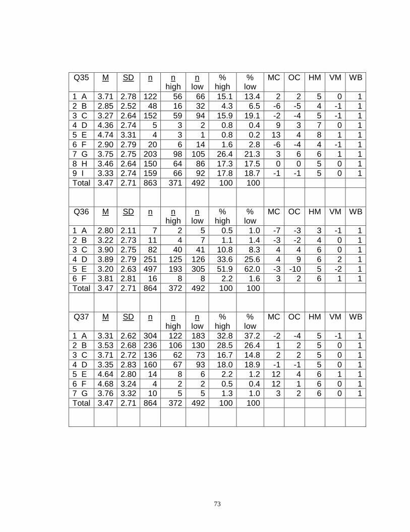
73
Q35 M SD n n high
n low
% high
% low
MC OC HM VM WB
1 A 3.71 2.78 122 56 66 15.1 13.4 2 2 5 0 1 2 B 2.85 2.52 48 16 32 4.3 6.5 -6 -5 4 -1 1 3 C 3.27 2.64 152 59 94 15.9 19.1 -2 -4 5 -1 1 4 D 4.36 2.74 5 3 2 0.8 0.4 9 3 7 0 1 5 E 4.74 3.31 4 3 1 0.8 0.2 13 4 8 1 1 6 F 2.90 2.79 20 6 14 1.6 2.8 -6 -4 4 -1 1 7 G 3.75 2.75 203 98 105 26.4 21.3 3 6 6 1 1 8 H 3.46 2.64 150 64 86 17.3 17.5 0 0 5 0 1 9 I 3.33 2.74 159 66 92 17.8 18.7 -1 -1 5 0 1 Total 3.47 2.71 863 371 492 100 100
Q36 M SD n n high
n low
% high
% low
MC OC HM VM WB
1 A 2.80 2.11 7 2 5 0.5 1.0 -7 -3 3 -1 1 2 B 3.22 2.73 11 4 7 1.1 1.4 -3 -2 4 0 1 3 C 3.90 2.75 82 40 41 10.8 8.3 4 4 6 0 1 4 D 3.89 2.79 251 125 126 33.6 25.6 4 9 6 2 1 5 E 3.20 2.63 497 193 305 51.9 62.0 -3 -10 5 -2 1 6 F 3.81 2.81 16 8 8 2.2 1.6 3 2 6 1 1 Total 3.47 2.71 864 372 492 100 100
Q37 M SD n n high
n low
% high
% low
MC OC HM VM WB
1 A 3.31 2.62 304 122 183 32.8 37.2 -2 -4 5 -1 1 2 B 3.53 2.68 236 106 130 28.5 26.4 1 2 5 0 1 3 C 3.71 2.72 136 62 73 16.7 14.8 2 2 5 0 1 4 D 3.35 2.83 160 67 93 18.0 18.9 -1 -1 5 0 1 5 E 4.64 2.80 14 8 6 2.2 1.2 12 4 6 1 1 6 F 4.68 3.24 4 2 2 0.5 0.4 12 1 6 0 1 7 G 3.76 3.32 10 5 5 1.3 1.0 3 2 6 0 1 Total 3.47 2.71 864 372 492 100 100

74
Q38 M SD n n high
n low
% high
% low
MC OC HM VM WB
1 A 3.44 2.71 386 167 220 44.9 44.6 0 0 5 0 1 2 B 3.59 2.61 204 91 113 24.5 22.9 1 2 5 0 1 3 C 3.67 2.85 92 41 51 11.0 10.3 2 1 5 0 1 4 D 3.26 2.70 142 55 87 14.8 17.6 -2 -4 5 -1 1 5 E 3.45 2.93 25 11 13 3.0 2.6 0 0 5 0 1 6 F 3.32 3.44 6 2 4 0.5 0.8 -1 -2 4 0 1 7 G 3.35 2.79 10 5 5 1.3 1.0 -1 2 6 0 1 Total 3.47 2.71 865 372 493 100.0 100.0
Q39 M SD n n high
n low
% high
% low
MC OC HM VM WB
1 A 3.44 2.73 431 184 246 49.6 50.0 0 -1 5 0 1 2 B 3.63 2.72 209 93 116 25.1 23.6 2 2 5 0 1 3 C 3.27 2.66 185 75 111 20.2 22.6 -2 -3 5 0 1 4 D 3.81 2.58 38 19 19 5.1 3.9 3 3 6 0 1 Total 3.47 2.70 863 371 492 100 100
Q40 M SD n n high
n low
% high
% low
MC OC HM VM WB
1 A 3.50 2.69 585 256 329 69.0 66.9 0 2 5 0 1 2 B 3.29 2.73 220 89 131 24.0 26.6 -2 -3 5 -1 1 3 C 4.16 2.59 30 16 14 4.3 2.8 7 4 6 1 1 4 D 2.60 2.77 10 2 8 0.5 1.6 -9 -5 2 -1 1 5 E 1.23 0.21 2 0 2 0.0 0.4 -22 -4 0 0 1 6 F 4.00 3.09 16 8 8 2.2 1.6 5 2 6 1 1 Total 3.47 2.71 863 371 492 100 100

75
Q41 M SD n n high
n low
% high
% low
MC OC HM VM WB
1 A 3.86 2.79 271 135 137 36.3 27.8 4 9 6 2 1 2 B 3.37 2.64 388 163 223 43.8 45.3 -1 -1 5 0 1 3 C 3.09 2.61 165 57 108 15.3 22.0 -4 -8 4 -1 1 4 D 4.12 2.73 21 12 10 3.2 2.0 7 3 6 1 1 5 E 2.90 3.13 5 1 4 0.3 0.8 -6 -4 2 -1 1 6 F 0.73 0.34 3 0 3 0.0 0.6 -27 -5 0 -1 1 7 G 1.02 - 1 0 1 0.0 0.2 -25 -3 0 0 1 8 H 3.16 3.32 10 4 6 1.1 1.2 -3 -1 5 0 1 Total 3.47 2.71 864 372 492 100 100
Q42 M SD n n high
n low
% high
% low
MC OC HM VM WB
1 A 3.82 2.73 38 18 21 4.9 4.3 3 1 5 0 1 2 B 3.53 2.68 88 38 52 10.2 10.6 1 0 5 0 1 3 C 3.63 2.71 381 177 203 47.7 41.3 2 6 5 1 1 4 D 3.53 2.74 167 71 95 19.1 19.3 1 0 5 0 1 5 E 3.09 2.75 143 53 90 14.3 18.3 -4 -5 4 -1 1 6 F 2.68 2.31 46 14 31 3.8 6.3 -8 -6 4 -1 1 Total 3.47 2.71 863 371 492 100 100
Q43 M SD n n high
n low
% high
% low
MC OC HM VM WB
1 A 3.12 2.64 383 137 242 36.9 49.2 -3 -12 4 -3 1 2 B 3.58 2.70 227 106 121 28.6 24.6 1 4 5 1 1 3 C 4.09 2.66 138 77 63 20.8 12.8 6 11 6 2 1 4 D 3.35 2.90 40 17 23 4.6 4.7 -1 0 5 0 1 5 E 3.81 2.82 75 34 42 9.2 8.5 3 1 5 0 1 Total 3.47 2.71 863 371 492 100 100
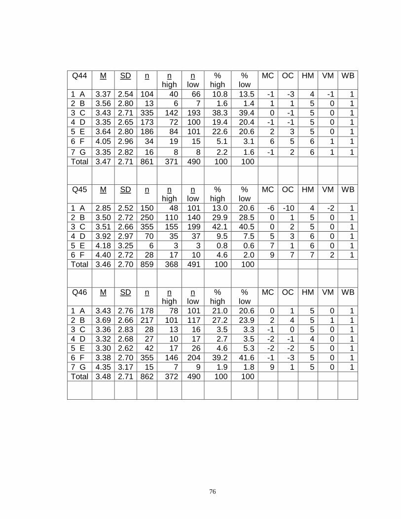
76
Q44 M SD n n high
n low
% high
% low
MC OC HM VM WB
1 A 3.37 2.54 104 40 66 10.8 13.5 -1 -3 4 -1 1 2 B 3.56 2.80 13 6 7 1.6 1.4 1 1 5 0 1 3 C 3.43 2.71 335 142 193 38.3 39.4 0 -1 5 0 1 4 D 3.35 2.65 173 72 100 19.4 20.4 -1 -1 5 0 1 5 E 3.64 2.80 186 84 101 22.6 20.6 2 3 5 0 1 6 F 4.05 2.96 34 19 15 5.1 3.1 6 5 6 1 1 7 G 3.35 2.82 16 8 8 2.2 1.6 -1 2 6 1 1 Total 3.47 2.71 861 371 490 100 100
Q45 M SD n n high
n low
% high
% low
MC OC HM VM WB
1 A 2.85 2.52 150 48 101 13.0 20.6 -6 -10 4 -2 1 2 B 3.50 2.72 250 110 140 29.9 28.5 0 1 5 0 1 3 C 3.51 2.66 355 155 199 42.1 40.5 0 2 5 0 1 4 D 3.92 2.97 70 35 37 9.5 7.5 5 3 6 0 1 5 E 4.18 3.25 6 3 3 0.8 0.6 7 1 6 0 1 6 F 4.40 2.72 28 17 10 4.6 2.0 9 7 7 2 1 Total 3.46 2.70 859 368 491 100 100
Q46 M SD n n high
n low
% high
% low
MC OC HM VM WB
1 A 3.43 2.76 178 78 101 21.0 20.6 0 1 5 0 1 2 B 3.69 2.66 217 101 117 27.2 23.9 2 4 5 1 1 3 C 3.36 2.83 28 13 16 3.5 3.3 -1 0 5 0 1 4 D 3.32 2.68 27 10 17 2.7 3.5 -2 -1 4 0 1 5 E 3.30 2.62 42 17 26 4.6 5.3 -2 -2 5 0 1 6 F 3.38 2.70 355 146 204 39.2 41.6 -1 -3 5 0 1 7 G 4.35 3.17 15 7 9 1.9 1.8 9 1 5 0 1 Total 3.48 2.71 862 372 490 100 100
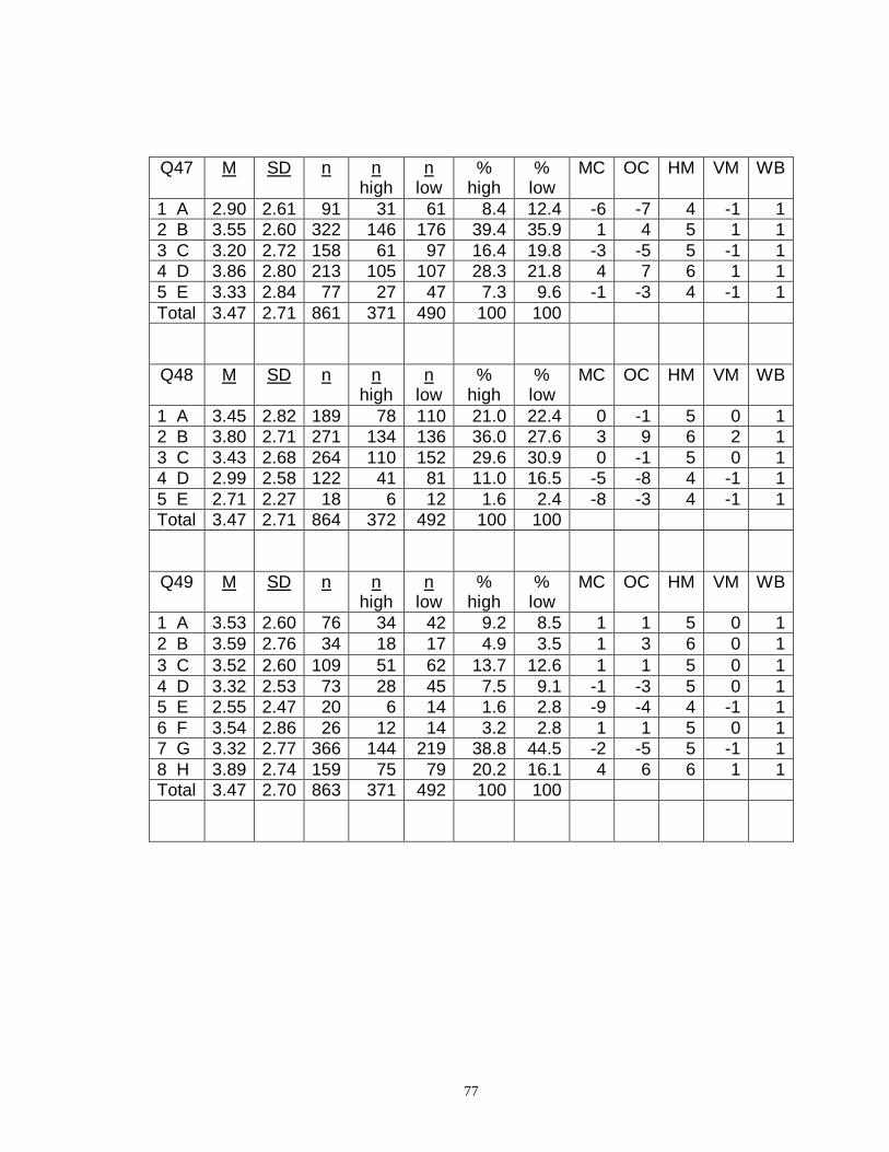
77
Q47 M SD n n high
n low
% high
% low
MC OC HM VM WB
1 A 2.90 2.61 91 31 61 8.4 12.4 -6 -7 4 -1 1 2 B 3.55 2.60 322 146 176 39.4 35.9 1 4 5 1 1 3 C 3.20 2.72 158 61 97 16.4 19.8 -3 -5 5 -1 1 4 D 3.86 2.80 213 105 107 28.3 21.8 4 7 6 1 1 5 E 3.33 2.84 77 27 47 7.3 9.6 -1 -3 4 -1 1 Total 3.47 2.71 861 371 490 100 100
Q48 M SD n n high
n low
% high
% low
MC OC HM VM WB
1 A 3.45 2.82 189 78 110 21.0 22.4 0 -1 5 0 1 2 B 3.80 2.71 271 134 136 36.0 27.6 3 9 6 2 1 3 C 3.43 2.68 264 110 152 29.6 30.9 0 -1 5 0 1 4 D 2.99 2.58 122 41 81 11.0 16.5 -5 -8 4 -1 1 5 E 2.71 2.27 18 6 12 1.6 2.4 -8 -3 4 -1 1 Total 3.47 2.71 864 372 492 100 100
Q49 M SD n n high
n low
% high
% low
MC OC HM VM WB
1 A 3.53 2.60 76 34 42 9.2 8.5 1 1 5 0 1 2 B 3.59 2.76 34 18 17 4.9 3.5 1 3 6 0 1 3 C 3.52 2.60 109 51 62 13.7 12.6 1 1 5 0 1 4 D 3.32 2.53 73 28 45 7.5 9.1 -1 -3 5 0 1 5 E 2.55 2.47 20 6 14 1.6 2.8 -9 -4 4 -1 1 6 F 3.54 2.86 26 12 14 3.2 2.8 1 1 5 0 1 7 G 3.32 2.77 366 144 219 38.8 44.5 -2 -5 5 -1 1 8 H 3.89 2.74 159 75 79 20.2 16.1 4 6 6 1 1 Total 3.47 2.70 863 371 492 100 100

78
Q50 M SD n n high
n low
% high
% low
MC OC HM VM WB
1 A 3.22 2.81 61 24 37 6.5 7.6 -3 -2 5 0 1 2 B 2.89 2.55 112 34 77 9.1 15.7 -6 -9 4 -1 1 3 C 3.29 2.69 200 78 121 21.0 24.7 -2 -4 5 -1 1 4 D 3.75 2.69 414 201 213 54.0 43.5 3 11 6 2 1 5 E 3.52 2.82 59 27 33 7.3 6.7 0 1 5 0 1 6 F 3.64 2.97 16 8 8 2.2 1.6 2 2 6 1 1 Total 3.48 2.71 862 372 490 100 100
Q51 M SD n n high
n low
% high
% low
MC OC HM VM WB
1 A 3.19 2.74 63 22 41 5.9 8.4 -3 -5 4 -1 1 2 B 3.84 2.78 101 52 49 14.0 10.0 4 6 6 1 1 3 C 3.70 2.73 401 190 211 51.1 43.0 2 8 5 2 1 4 D 3.08 2.62 226 79 147 21.2 29.9 -4 -10 4 -2 1 5 E 3.53 2.60 51 22 29 5.9 5.9 0 0 5 0 1 6 F 2.40 2.21 21 7 14 1.9 2.9 -11 -3 4 -1 1 Total 3.48 2.71 863 372 491 100 100
Q52 M SD n n high
n low
% high
% low
MC OC HM VM WB
1 A 3.32 2.68 202 81 121 21.8 24.6 -2 -3 5 -1 1 2 B 3.39 2.97 6 3 3 0.8 0.6 -1 1 6 0 1 3 C 3.54 2.67 220 98 122 26.3 24.8 1 2 5 0 1 4 D 3.36 2.80 203 83 120 22.3 24.4 -1 -2 5 0 1 5 E 3.99 2.73 114 58 56 15.6 11.4 5 6 6 1 1 6 F 3.10 2.57 59 21 38 5.6 7.7 -4 -4 4 -1 1 7 G 3.55 2.62 59 28 31 7.5 6.3 1 2 5 0 1 Total 3.48 2.71 863 372 491 100 100
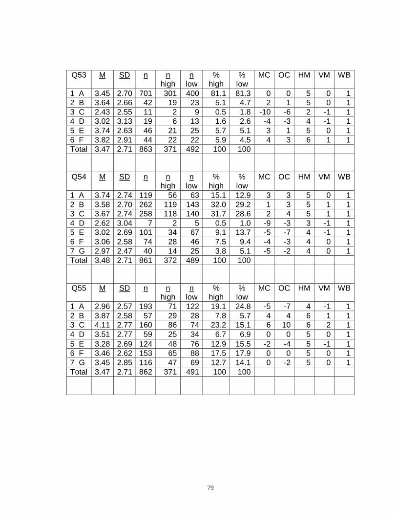
79
Q53 M SD n n high
n low
% high
% low
MC OC HM VM WB
1 A 3.45 2.70 701 301 400 81.1 81.3 0 0 5 0 1 2 B 3.64 2.66 42 19 23 5.1 4.7 2 1 5 0 1 3 C 2.43 2.55 11 2 9 0.5 1.8 -10 -6 2 -1 1 4 D 3.02 3.13 19 6 13 1.6 2.6 -4 -3 4 -1 1 5 E 3.74 2.63 46 21 25 5.7 5.1 3 1 5 0 1 6 F 3.82 2.91 44 22 22 5.9 4.5 4 3 6 1 1 Total 3.47 2.71 863 371 492 100 100
Q54 M SD n n high
n low
% high
% low
MC OC HM VM WB
1 A 3.74 2.74 119 56 63 15.1 12.9 3 3 5 0 1 2 B 3.58 2.70 262 119 143 32.0 29.2 1 3 5 1 1 3 C 3.67 2.74 258 118 140 31.7 28.6 2 4 5 1 1 4 D 2.62 3.04 7 2 5 0.5 1.0 -9 -3 3 -1 1 5 E 3.02 2.69 101 34 67 9.1 13.7 -5 -7 4 -1 1 6 F 3.06 2.58 74 28 46 7.5 9.4 -4 -3 4 0 1 7 G 2.97 2.47 40 14 25 3.8 5.1 -5 -2 4 0 1 Total 3.48 2.71 861 372 489 100 100
Q55 M SD n n high
n low
% high
% low
MC OC HM VM WB
1 A 2.96 2.57 193 71 122 19.1 24.8 -5 -7 4 -1 1 2 B 3.87 2.58 57 29 28 7.8 5.7 4 4 6 1 1 3 C 4.11 2.77 160 86 74 23.2 15.1 6 10 6 2 1 4 D 3.51 2.77 59 25 34 6.7 6.9 0 0 5 0 1 5 E 3.28 2.69 124 48 76 12.9 15.5 -2 -4 5 -1 1 6 F 3.46 2.62 153 65 88 17.5 17.9 0 0 5 0 1 7 G 3.45 2.85 116 47 69 12.7 14.1 0 -2 5 0 1 Total 3.47 2.71 862 371 491 100 100

80
Q56 M SD n n high
n low
% high
% low
MC OC HM VM WB
1 A 3.48 2.72 481 209 272 56.2 55.3 0 1 5 0 1 2 B 2.62 2.30 11 4 7 1.1 1.4 -9 -2 4 0 1 3 C 2.96 2.60 28 9 19 2.4 3.9 -5 -4 4 -1 1 4 D 3.78 2.67 137 67 70 18.0 14.2 3 5 6 1 1 5 E 3.49 2.74 28 10 18 2.7 3.7 0 -3 4 0 1 6 F 3.21 2.76 119 46 73 12.4 14.8 -3 -4 5 -1 1 7 G 3.61 2.67 60 26 33 7.0 6.7 1 1 5 0 1 Total 3.47 2.71 864 372 492 100 100
Q57 M SD n n high
n low
% high
% low
MC OC HM VM WB
1 A 3.44 2.70 521 225 296 60.5 60.2 0 0 5 0 1 2 B 3.50 2.66 248 105 143 28.2 29.1 0 -1 5 0 1 3 C 4.03 2.73 13 7 6 1.9 1.2 6 3 6 1 1 4 D 1.94 3.00 5 1 4 0.3 0.8 -15 -4 2 -1 1 5 E 3.62 2.86 77 34 43 9.1 8.7 1 1 5 0 1 Total 3.47 2.71 864 372 492 100 100
Q58 M SD n n high
n low
% high
% low
MC OC HM VM WB
1 A 3.38 2.75 258 109 149 29.3 30.3 -1 -1 5 0 1 2 B 3.51 2.66 507 220 287 59.1 58.5 0 1 5 0 1 3 C 3.85 2.89 64 30 34 8.1 6.9 4 2 5 0 1 4 D 2.79 2.94 5 2 3 0.5 0.6 -7 0 5 0 1 5 E 0.52 0.49 4 0 4 0.0 0.8 -30 -6 0 -1 1 6 F 3.37 2.66 25 11 14 3.0 2.9 -1 0 5 0 1 Total 3.48 2.70 863 372 491 100 100
Q59 M SD n n high
n low
% high
% low
MC OC HM VM WB
1 A 3.83 2.85 233 118 115 31.8 23.4 4 9 6 2 1 2 B 3.29 2.65 274 105 169 28.3 34.4 -2 -6 5 -1 1 3 C 3.55 2.68 271 121 150 32.6 30.5 1 2 5 0 1 4 D 2.84 2.43 84 27 57 7.3 11.6 -6 -7 4 -2 1 Total 3.47 2.70 862 371 491 100 100

81
Q60 M SD n n high
n low
% high
% low
MC OC HM VM WB
1 A 1.94 2.07 7 1 6 0.3 1.2 -15 -5 2 -1 1 2 B 3.20 3.33 7 2 5 0.5 1.0 -2 -3 3 -1 1 3 C 3.92 3.00 18 9 9 2.5 1.8 5 2 6 1 1 4 D 3.49 2.72 53 22 31 6.0 6.3 0 -1 5 0 1 5 E 3.43 2.70 717 305 412 83.3 83.9 0 -2 5 0 1 6 F 3.75 2.64 55 27 27 7.4 5.5 3 3 6 1 1 Total 3.45 2.71 857 366 491 100 100
Q61 M SD n n high
n low
% high
% low
MC OC HM VM WB
1 A 3.53 2.70 759 335 424 91.0 86.7 1 6 5 1 1 2 B 3.52 2.92 31 12 19 3.3 3.9 0 -2 5 0 1 3 C 2.72 2.66 28 9 19 2.4 3.9 -8 -4 4 -1 1 4 D 2.95 2.94 19 6 13 1.6 2.7 -5 -3 4 -1 1 5 E 2.79 2.56 20 6 14 1.6 2.9 -7 -4 4 -1 1 Total 3.47 2.71 857 368 489 100 100
Q62 M SD n n high
n low
% high
% low
MC OC HM VM WB
1 A 3.62 2.72 493 221 272 59.7 55.6 1 4 5 1 1 2 B 4.22 2.66 37 21 16 5.7 3.3 7 6 6 1 1 3 C 3.10 2.89 60 25 35 6.8 7.2 -4 -1 5 0 1 4 D 3.31 2.67 143 58 84 15.7 17.2 -2 -2 5 0 1 5 E 3.23 2.59 31 13 19 3.5 3.9 -2 -2 5 0 1 6 F 3.01 2.57 95 32 63 8.6 12.9 -5 -7 4 -1 1 Total 3.48 2.71 859 370 489 100 100

82
Q63 M SD n n high
n low
% high
% low
MC OC HM VM WB
1 A 3.89 2.71 57 31 26 8.4 5.3 4 6 6 1 1 2 B 3.56 2.69 365 160 205 43.4 41.8 1 1 5 0 1 3 C 3.54 2.75 44 19 25 5.1 5.1 1 0 5 0 1 4 D 3.25 2.63 63 26 37 7.0 7.6 -2 -1 5 0 1 5 E 3.33 2.74 330 132 197 35.8 40.2 -1 -4 5 -1 1 Total 3.47 2.71 859 369 490 100 100
Note. M = Mean retention rate in months for all the incumbents who selected the option.
n high = number of incumbents in the high criterion group who selected the item
response option. n low = number of incumbents in the low criterion group who selected
the item response option. % high = percentage of incumbents in high criterion group who
selected the item response option. % low = percentage of incumbents in low criterion
group who selected the item response option. MC = Mean Standardized Criterion scoring
weights. OC = Option Criterion Correlation scoring weights. HM = Horizontal
Percentage Method scoring weights. VM = Vertical Percentage Method Scoring weights.
WB = Weighted Application Blank scoring weights.

83
APPENDIX B
WHITE AND NON MINORITY RACE SELECTION PERCENTAGE RATES OF THE
HOLDOUT SAMPLE FOR EACH OF THE FOUR METHODS

84
WHITE AND NON-WHITE RACE SELECTION PERCENTAGE RATES OF THE
HOLDOUT SAMPLE FOR EACH OF THE FOUR METHODS
Race
Scoring Methods Non-White
n = 200
White
n = 234
AI Ratio
OCC .53 .82 .65
MSC .59 .81 .73
HPM .62 .83 .75
VPM .59 .82 .72
Note. Selection rates are rounded to nearest whole percent. AI Ratio = Adverse impact
ratio. The lower selection rate is divided by the larger selection rate to determine the AI
Ratio. AI Ratio ? .80 means no adverse impact.

85
APPENDIX C
TESTING FOR SIGNIFICANT DIFFERENCES BETWEEN THE MEAN ITEM
SCORING WEIGHTS FOR WHITES AND BLACKS FOR RACIAL ADVERSE
IMPACT FOR EACH OF THE FOUR METHODS

86
TESTING FOR SIGNIFICANT DIFFERENCES BETWEEN THE MEAN ITEM
SCORING WEIGHTS FOR WHITES AND BLACKS FOR RACIAL ADVERSE
IMPACT FOR EACH OF THE FOUR METHODS
OCC MSC HPM VPM Item # M SD M SD M SD M SD
Q1 White -0.17** 4.64 -0.97** 2.36 4.60** 0.63 -0.05** 0.82 Black 0.96** 4.46 -0.45** 2.41 4.72** 0.48 0.15** 0.81 Q2 White -0.72 4.19 -0.21 1.93 5.24 0.44 -0.54 0.84 Black -0.15 4.51 -0.07 1.80 5.29 0.46 -0.43 0.90 Q3 White 0.10 4.36 -0.17 3.02 5.08 0.58 0.08 0.58 Black -0.08 4.45 -0.38 3.09 5.06 0.59 0.06 0.59 Q4 White 4.30 5.85 0.55 3.15 4.72 0.83 0.93 1.33 Black 4.37 5.63 0.36 3.14 4.79 0.70 0.96 1.26 Q5 White -1.44 4.55 0.01 2.49 4.77 0.65 -0.08* 0.79 Black -0.81 4.24 -0.06 2.02 4.82 0.56 0.06* 0.76 Q6 White 1.15 6.62 -0.21 4.23 5.15 0.71 0.19 1.33 Black 1.78 6.83 0.13 4.31 5.16 0.80 0.30 1.36 Q7 White -0.78 4.80 -0.34* 3.11 4.97 0.63 -0.11 0.98 Black -0.04 5.01 0.19* 2.80 5.05 0.49 0.00 0.97 Q8 White 0.73 2.61 0.16 2.21 4.90 0.48 0.01 0.37 Black 0.61 2.62 0.01 2.06 4.86 0.43 -0.04 0.32 Q9 White -1.02** 4.28 -0.47** 2.52 4.79* 0.60 -0.15** 0.57 Black 0.09** 3.95 0.65** 3.36 4.92* 0.77 0.01** 0.58

87
OCC MSC HPM VPM Item # M SD M SD M SD M SD
Q10 White 0.17 1.51 0.21 1.58 5.12 0.32 0.00 0.00 Black 0.28 1.77 0.32 1.75 5.16 0.37 0.00 0.00 Q11 White -0.31 1.15 -0.07 0.85 5.00 0.00 0.00 0.00 Black -0.48 1.18 -0.20 0.94 5.01 0.13 0.00 0.00 Q12 White -1.47 2.42 -0.05 1.97 5.13 0.34 -0.47 0.72 Black -1.21 2.60 0.15 2.25 5.15 0.51 -0.38 0.76 Q13 White 0.51 6.86 -0.27 4.27 5.10 0.85 0.45 1.20 Black 0.58 6.33 -0.21 4.30 5.07 0.84 0.44 1.12 Q14 White 0.08 2.03 -0.05 1.96 4.99 0.34 -0.06 0.25 Black 0.43 2.33 0.21 2.12 4.94 0.39 -0.11 0.31 Q15 White 0.36 4.12 0.16 3.18 5.17 0.61 0.17 0.61 Black 0.54 4.28 0.12 3.17 5.18 0.66 0.18 0.66 Q16 White -1.69 4.48 -0.47 1.89 5.16 0.37 -0.62 0.75 Black -1.27 4.61 -0.23 2.07 5.19 0.39 -0.56 0.80 Q17 White -0.15* 1.57 0.27** 1.21 5.00 0.00 0.00 0.00 Black -0.42* 1.58 -0.06** 1.13 5.00 0.00 0.00 0.00 Q18 White -1.80 4.85 0.17 4.29 5.09 0.65 -0.53 0.73 Black -1.33 5.37 0.53 4.40 5.07 0.85 -0.49 0.77 Q19 White 0.56** 3.81 -0.74** 2.54 4.85 0.61 0.35 0.74 Black 1.45** 4.00 0.11** 3.19 4.87 0.91 0.46 0.76 Q20 White 0.49 4.93 -0.02 1.95 4.92 0.61 0.04 0.82 Black 0.71 5.01 0.05 2.06 4.97 0.28 0.08 0.84 Q21 White -0.99** 8.19 -0.55** 4.93 4.78** 1.15 0.03** 1.31 Black 1.41** 9.80 0.90** 5.69 5.08** 1.32 0.43** 1.54

88
OCC MSC HPM VPM Item # M SD M SD M SD M SD
Q22 White 2.01 9.55 -0.15 3.01 5.21 0.83 0.90 2.00 Black 2.74 9.49 0.03 3.04 5.27 0.82 1.04 2.00 Q23 White -0.39** 3.77 -0.41 1.83 4.69 0.69 -0.05** 0.66 Black 0.48** 4.08 -0.18 1.92 4.76 0.52 0.12** 0.73 Q24 White -2.35** 3.29 -0.16** 2.46 5.07** 0.70 -0.74** 0.71 Black -0.84** 4.53 0.95** 3.55 5.32** 0.57 -0.42** 0.99 Q25 White -0.78 2.80 -0.41 1.75 5.07 0.67 -0.21 0.41 Black -0.68 2.79 -0.12 2.00 5.10 0.30 -0.18 0.47 Q26 White 0.39 4.43 -0.15 3.43 4.69** 0.79 -0.07** 0.85 Black 0.88 4.08 0.30 2.78 4.84** 0.55 0.10** 0.75 Q27 White -0.26 3.86 -0.15 3.46 4.92 0.86 0.19 0.78 Black -0.54 4.59 -0.44 4.48 4.94 0.87 0.09 0.96 Q28 White 0.19 0.94 0.24 1.02 5.00 0.23 0.03 0.16 Black 0.26 0.95 0.27 0.99 4.99 0.22 0.02 0.13 Q29 White 0.78* 5.80 0.16 3.02 4.72 0.87 0.14 0.91 Black 1.76* 5.68 0.48 2.77 4.75 0.79 0.29 0.86 Q30 White 5.67 7.83 0.19 3.22 4.65 0.63 1.02 1.46 Black 5.72 7.89 0.26 2.97 4.68 0.56 1.03 1.46 Q31 White -0.94 5.01 0.27* 3.72 5.06 0.57 -0.12 1.08 Black -0.22 4.93 0.97* 4.25 5.15 0.69 0.06 1.05 Q32 White 0.20 4.24 0.26 1.29 5.03 0.70 0.17 0.98 Black -0.44 4.32 0.12 1.26 5.06 0.39 0.01 0.99 Q33 White 1.01 6.33 0.15* 2.76 5.22* 0.77 0.32 1.47 Black 1.84 5.88 0.63* 2.41 5.35* 0.66 0.43 1.46

89
OCC MSC HPM VPM Item # M SD M SD M SD M SD
Q34 White -0.29** 5.89 -1.69** 3.81 4.66** 0.57 -0.08** 1.47 Black 2.09** 5.32 0.01** 2.64 4.82** 0.46 0.65** 1.35 Q35 White 0.09* 3.50 -0.12 2.70 5.12* 0.55 -0.08** 0.66 Black 0.82* 3.92 0.28 3.31 5.24* 0.71 0.06** 0.73 Q36 White -4.42** 8.08 -0.87** 3.27 5.27** 0.54 -0.92** 1.63 Black -2.01** 8.74 0.15** 3.52 5.44** 0.55 -0.43** 1.79 Q37 White -1.10 2.86 -0.32 2.15 4.97 0.59 -0.45** 0.52 Black -0.84 2.65 -0.13 2.48 5.00 0.36 -0.34** 0.51 Q38 White 0.14 1.69 0.08 0.95 5.00 0.44 -0.11* 0.31 Black 0.01 2.01 0.18 1.20 5.00 0.07 -0.17* 0.38 Q39 White -0.36 1.96 0.29 1.53 5.00 0.44 0.00 0.00 Black -0.23 2.05 0.38 1.61 5.06 0.23 0.00 0.00 Q40 White 1.08** 2.06 -0.15 1.73 5.03 0.32 -0.15 0.47 Black 0.54** 2.42 -0.18 2.12 5.06 0.33 -0.23 0.58 Q41 White 0.00** 5.89 -0.32 3.10 5.00 0.84 0.29** 1.07 Black 1.46** 6.19 0.15 3.90 5.14 0.90 0.56** 1.15 Q42 White 0.42** 4.33 -0.33** 3.37 4.73 0.44 0.03** 0.76 Black 1.59** 4.36 0.33** 2.66 4.79 0.41 0.23** 0.77 Q43 White -4.08** 8.72 -0.44** 3.07 4.54** 0.76 -1.12** 2.04 Black -1.00** 9.18 0.74** 3.49 4.85** 0.76 -0.44** 2.08 Q44 White -0.31** 1.95 0.09** 1.30 5.02 0.14 0.02** 0.14 Black 0.20** 2.26 0.56** 1.72 5.03 0.54 0.07** 0.26 Q45 White -2.04** 5.85 -1.38** 3.92 4.80** 0.73 -0.54** 1.14 Black 0.83** 3.54 0.50** 3.00 5.09** 0.65 0.01** 0.77

90
OCC MSC HPM VPM Item # M SD M SD M SD M SD
Q46 White -0.87** 2.72 -0.37** 1.22 4.87 0.61 -0.35** 0.77 Black 0.32** 2.98 0.30** 1.80 4.96 0.36 -0.05** 0.84 Q47 White 0.56* 5.32 -0.24 3.14 4.74 0.89 0.17** 0.94 Black 1.55* 5.11 0.20 3.13 4.88 0.83 0.40** 0.86 Q48 White 0.72* 5.82 -0.26** 3.05 5.09 0.69 0.38* 1.10 Black 1.77* 5.70 0.35** 2.68 5.21 0.74 0.58* 1.09 Q49 White -1.40 4.02 -0.58 2.85 5.08 0.75 -0.35* 0.71 Black -0.94 4.06 -0.13 2.58 5.07 0.87 -0.23* 0.71 Q50 White 2.90 7.82 -0.10 3.33 5.29 0.94 0.63 1.33 Black 3.63 7.75 0.29 3.13 5.39 0.84 0.70 1.38 Q51 White -0.68** 7.98 -1.01** 3.44 4.56** 0.71 -0.01** 1.76 Black 1.59** 7.64 0.04** 3.32 4.76** 0.75 0.47** 1.68 Q52 White 0.21 2.97 0.07 2.20 4.97 0.69 -0.18 0.58 Black 0.21 3.09 0.10 2.35 5.03 0.56 -0.12 0.59 Q53 White -0.02 1.36 0.06 2.18 4.90 0.69 -0.01 0.34 Black -0.02 1.19 0.03 1.92 4.93 0.60 -0.01 0.29 Q54 White 0.39* 4.36 -0.53 3.26 4.62 0.63 0.31* 0.82 Black 1.14* 3.90 0.00 2.93 4.71 0.55 0.47* 0.74 Q55 White -1.87** 4.65 -1.04** 3.21 4.81** 0.74 -0.22** 0.85 Black 0.38** 5.72 0.41** 3.69 5.08** 0.76 0.20** 1.07 Q56 White 0.57 2.93 -0.15 2.15 5.08 0.74 -0.03 0.64 Black 0.53 2.66 -0.12 1.95 5.06 0.56 -0.04 0.57 Q57 White -0.22 0.70 0.02 1.33 4.96 0.47 0.00 0.11 Black -0.16 0.71 0.09 1.23 4.98 0.40 0.01 0.13
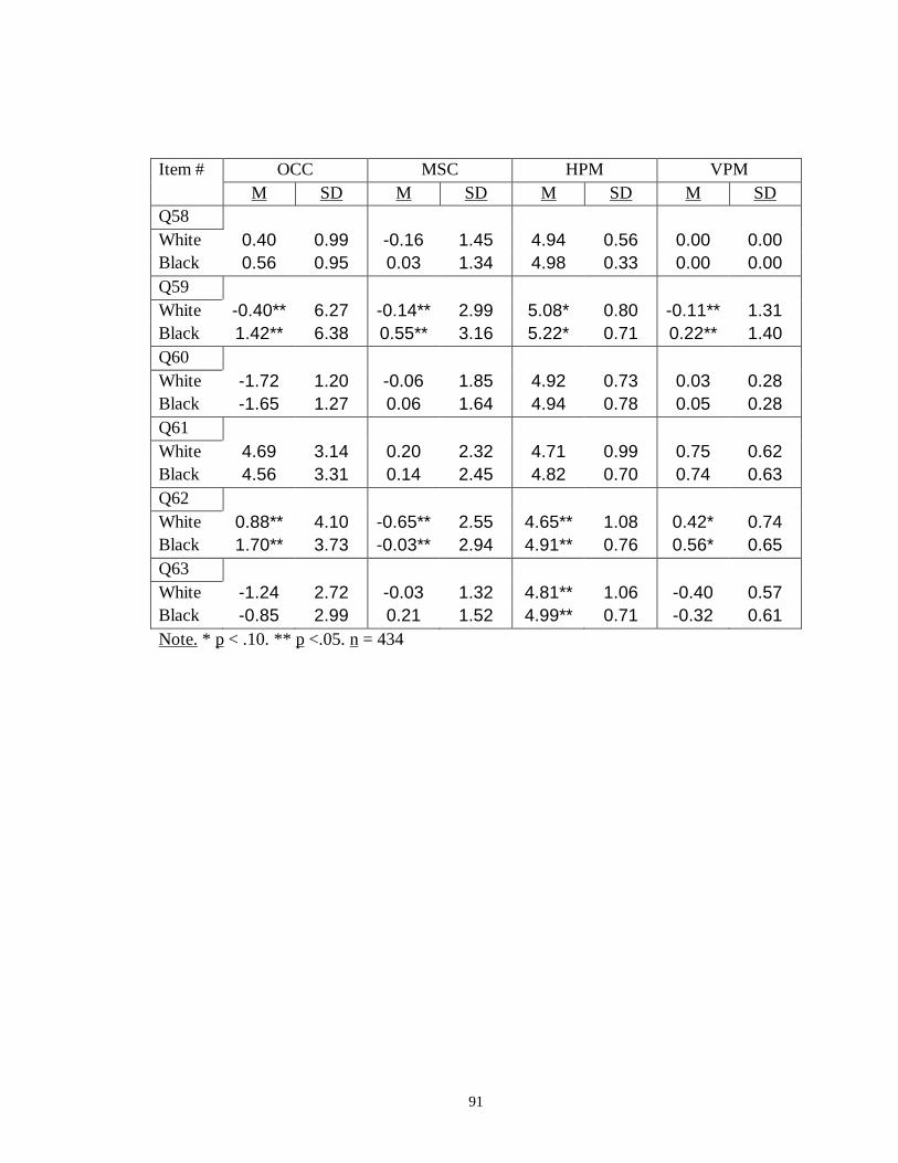
91
OCC MSC HPM VPM Item # M SD M SD M SD M SD
Q58 White 0.40 0.99 -0.16 1.45 4.94 0.56 0.00 0.00 Black 0.56 0.95 0.03 1.34 4.98 0.33 0.00 0.00 Q59 White -0.40** 6.27 -0.14** 2.99 5.08* 0.80 -0.11** 1.31 Black 1.42** 6.38 0.55** 3.16 5.22* 0.71 0.22** 1.40 Q60 White -1.72 1.20 -0.06 1.85 4.92 0.73 0.03 0.28 Black -1.65 1.27 0.06 1.64 4.94 0.78 0.05 0.28 Q61 White 4.69 3.14 0.20 2.32 4.71 0.99 0.75 0.62 Black 4.56 3.31 0.14 2.45 4.82 0.70 0.74 0.63 Q62 White 0.88** 4.10 -0.65** 2.55 4.65** 1.08 0.42* 0.74 Black 1.70** 3.73 -0.03** 2.94 4.91** 0.76 0.56* 0.65 Q63 White -1.24 2.72 -0.03 1.32 4.81** 1.06 -0.40 0.57 Black -0.85 2.99 0.21 1.52 4.99** 0.71 -0.32 0.61 Note. * p < .10. ** p <.05. n = 434

92
References
Allworth, E. (1999, August 13). Using Biodata [on-line]. Retrieved January, 2,
2001 from www.pai.org.za/biodata.htm.
Anastasi, A. (1980). Psychological testing and privacy. In W.C. Bier (Ed).
Privacy a vanishing value? New York: Fordham University Press.
Appel, V., & Feinberg, M.R. (1969). Recruiting door-to-door salesmen by mail.
Journal of Applied Psychology, 53, 362-366.
Arnold, D.W. (1990, October). Invasion of privacy: A rising concern for
personnel psychologists. The Industrial/Organizational Psychologist, 28, 37-39.
Ashforth, B.E., & Mael, M. (1989). Social Identity Theory and the organization.
Academy of Management Review, 14(1), 20-39.
Barrett, G.V., Alexander, R.A., & Doverspike, D. (1992). The implication for
personnel selection of apparent declines in predictive validities over time: A critique of
Hulin, Henry, and Noon. Personnel Psychology, 45, 601-617.
Becker, T.E., & Colquitt, A.L. (1992). Potential versus actual faking of a biodata
form: An analysis along several dimensions of item type. Personnel Psychology, 45(2),
389-405.
Brown, S.H. (1978). Long-term validity of a personal history item scoring
procedure. Journal of Applied Psychology, 63, 673-676.

93
Brown, S.H. (1994). Validating biodata. In G.S. Stokes, M.D. Mumford, & W.A.
Owens, (Eds.)., Biodata handbook: Theory, research, and use of biographical information
in selection and performance prediction (pp. 199-236). Palo Alto, CA: Consulting
Psychologists Press.
Brown, S.H., Corrigan, J.E., Stout, J.D., & Dalessio, A.T. (1987, August). The
transportability of biodata keys across English-speaking cultures. Paper presented at the
annual meeting of the American Psychological Association, New York.
Brumback, G.B. (1969). A note on criterion contamination in the validation of
biographical data. Educational and Psychological Measurement, 29, 439-443.
Campbell, J.P., Dunnette, M.D., Lawler, E.E., & Weick, K. (1970). Managerial
behavior and performance effectiveness. New York: McGraw-Hill.
Carlson, K.D., Scullen, S.E., Schmidt, F.L., Rothstein, H., Erwin, F. (1999).
Generalizable biographical data validity can be achieved without multi-organizational
development and keying. Personnel Psychology, 52(3), 731-755.
Carraher, S.M., Mendoza, J.L., Buckley, M.R., Schoenfeldt, L.F., & Carraher,
C.E. (1998). Validation of an instrument to measure service-orientation. Journal of
Quality Management, 3(2), 211-224.
Cascio, W.F. (1975). Accuracy of verifiable biographical information blank
responses. Journal of Applied Psychology, 60, 767-776.
Cascio, W.F. (1992). Managing Human Resources. New York: McGraw-Hill.
Chait, H.N., Carraher, S.M., & Buckley, M.R. (2000). Measuring service
orientation with biodata. Journal of Managerial Issues, 12(1), 109-120.

94
Collins, J.M., & Schmidt, F.L. (1993). Personality, integrity, and white-collar
crime: A construct validity study. Personnel Psychology, 46(2), 295-311.
Constanza, D.P., & Mumford, M.D. (1993). Prediction of state department
assessment center performance using biodata job dimension scales. Fairfax, VA: Center
for Behavioral and Cognitive Studies.
Crafts, Jennifer (1991). Using biodata as a selection instrument. ERIC/TM
Digest.[on-line]. Retrieved December, 19, 2000 from
www.ericae.net/db/edo/ED338702.htm.
Cureton, E.E. (1965) Comment. In E.P. Henry (Ed.) Research conference on the
use of autobiographical data as psychological predictors (p.13). Greensboro, NC:
Richardson Foundation.
Dean, M.A., & Russell, C.J. (1998, April). A comparison of g and biodata
criterion-related validity in a sample of air traffic controllers. Paper presented at the 13th
Annual Conference of the Society for Industrial and Organizational Psychology, Dallas,
TX.
Dickinson, A., & Ineson, E.M. (1993). The selection of quality operative staff in
the hotel sector. International Journal of Contemporary Hospitality Management, 5(1),
16-21.
Doll, R.E. (1971). Item susceptibility to attempted faking as related to item
characteristics and adopted fake set. Journal of Psychology, 77, 9-16.
Dreher, G.F., & Sackett, P.R. (1983). Perspectives on staffing and selection.
Homewood, IL: Irwin.
95
Dunnette, M.D. (1962). Personnel management. Annual Review of Psychology,
13, 285-314.
England, G.W. (1961). Development and use of weighted application blanks.
Dubuque, IA: Brown.
England, G.W. (1971). Development and use of weighted application blanks
(Bulletin No.55, rev.ed.). Minneapolis: University of Minnesota, Industrial Relations
Center.
Fletcher, C. (1992). Ethics: The job interview. Personnel Management, 24(3), 36-
39.
Goldstein, I.L. (1971). The application blank: How honest are the responses?
Journal of Applied Psychology, 55, 491-492.
Hallis release latest study into agent turnover in Australian centres. (1999,
December 22). [on-line]. Retrieved August, 16, 2000 from
/http://www.apccn.com/webx?archivepage@@.
Hammer, E.G., & Kleiman, L.A. (1988, May). Getting to know you. Personnel
Administrator, 33, 86-92.
Harvey-Cook, J.E. (2000). Biodata in professional entry-level selection: Statistical
scoring of common format applications. Journal of Occupational and Organizational
Psychology, 73 (1), 103-118.

96
Hogan, J.B. (1988). The influence of socially desirable responding on
biographical data of applicant versus incumbent samples: implications for predictive and
concurrent research designs. Unpublished doctoral dissertation, University of Georgia,
Athens.
Hogan, J.B. (1994). Empirical keying of background measures. In G.S. Stokes,
M.D. Mumford, & W.A. Owens, (Eds.)., Biodata handbook: Theory, research, and use of
biographical information in selection and performance prediction (pp. 69-107) .Palo Alto,
CA: Consulting Psychologists Press.
Huffcut, A.I., Roth, P.L., & McDaniel, M.A. (1996). A meta-analytic
investigation of cognitive ability in employment interview evaluations: Moderating
characteristics and implications for incremental validity. Journal of Applied Psychology,
79, 599-616.
Hunter, J.E. (1980). Validity generalization for 12,000 jobs: An application of
synthetic validity and validity generalization to the General Aptitude Test Battery
(GATB). Washington, D.C.: U.S. Department of Labor and Employment Service.
Hunter, J.E. (1986). Cognitive ability, cognitive aptitudes, job knowledge, and job
performance. Journal of Vocational Behavior, 29, 340-362.
Hunter, J.E., & Hunter, R.F. (1984). Validity and utility of alternative predictors
of job performance. Psychological Bulletin, 96, 72-99.
Hunter, J.E., & Schmidt, F.L. (1996). Intelligence and job performance:
Economic and social implications. Psychology, Public Policy, and Law, 2, 447-472.

97
Kluger, A.N., Reilly, R.R., & Russell, C.J. (1991). Faking biodata tests: Are
option-keyed instruments more resistant? Journal of Applied Psychology, 76, 889-896.
Kluger, A.N., & Rothstein, H.R. (1993). The influence of selection test type on
applicants’ reactions to employment testing. Journal of Business and Psychology, 8, 3-25.
Korman, A.K. (1971). Industrial and Organizational Psychology (p.239). New
York: Prentice-Hall.
Lautenschlager, G.J. (1994). Accuracy and faking of background data. In G.S.
Stokes, M.D. Mumford, & W.A. Owens, (Eds.)., Biodata handbook: Theory, research,
and use of biographical information in selection and performance prediction (pp. 391-
419). Palo Alto, CA: Consulting Psychologists Press.
Lecznar, W.B., & Dailey, J.T. (1950). Keying biographical inventories in
classification test batteries. American Psychologist, 5, 279.
Levin, G. (2000, May). Key aspects of successful agent retention process. Call
Center Management Review, 1,3-5, 19.
Mael, F.A. (1991). A conceptual rationale for the domain and attributes of biodata
items. Personnel Psychology, 44, 763-792.
Mael, F.A., & Ashforth, B.E. (1995). Loyal from day one: biodata, organizational
identification, and turnover among newcomers. Personnel Psychology, 48, 309-333.
Mael, F.A., Connerley, M., & Morath, R.A. (1996). None of your business:
Parameters of biodata invasiveness. Personnel Psychology, 49, 613-650.
Mael, F. A., & Hirsch, A.C. (1993). Rainforest empiricism and quasi-rationality:
Two-approaches to objective biodata. Personnel Psychology, 46(4), 719-738.

98
McDaniel, M.A., Whetzel, D.L., Schmidt, F.L., & Mauer, S.D. (1994). The
validity of employment interviews: a comprehensive review and meta-analysis. Journal
of Applied Psychology, 79, 599-616.
McManus, M.A., & Kelly, M.L. (1999). Personality measures and biodata:
Evidence regarding their incremental predictive value in the life insurance industry.
Personnel Psychology, 52(1), 137-148.
Melamed, T. (1992). Use of biodata for prediction academic success or thirty
years. Psychological Reports, 71, 31-38.
Mitchell, T.W. (1990). Can biodata predict personality? Proceedings of the 14th
Annual Conference of the International Personnel Management Assessment Council
(IPMAAC), San Diego.
Mitchell, T.W. (1992, May). A priori biodata to predict teamwork, learning rate,
and retention. Paper presented at the annual meeting of the Society of Industrial and
Organizational Psychology, Montreal, Canada.
Mitchell, T.W. (1994). The utility of biodata. In G.S. Stokes, M.D. Mumford, &
W.A. Owens, (Eds.)., Biodata handbook: Theory, research, and use of biographical
information in selection and performance prediction (pp. 485-516). Palo Alto, CA:
Consulting Psychologists Press.
Mitchell, T.W. (1998, April). The utility and practical value of biodata.
Symposium conducted at the annual meeting of the society for Industrial and
Organizational Psychology, Dallas.

99
Mitchell, TW. (2000). Fire fighter biodata: Summary of validity and fairness.
[On-line] San Diego CA. Retrieved May, 15, 2001 from www.e-Selex.com.
Mitchell, T.W., & Klimoski, R.J. (1982). Is it rational to be empirical? A test of
methods for scoring biographical data. Journal of Applied Psychology, 76, 411-418.
Morrison, R.F. (1994). Biodata applications in career development research and
practice. In G.S. Stokes, M.D. Mumford, & W.A. Owens, (Eds.)., Biodata handbook:
Theory, research, and use of biographical information in selection and performance
prediction (pp. 451-484). Palo Alto, CA: Consulting Psychologists Press.
Mount, M.K., & Barrick, M.R. (1995). The Big Five personality dimensions:
implications for research and practice in human resources management. In G.R. Ferris
(Eds.). Research in Personnel and Human Resources Management, 13, 153-200. JAI
Press.
Mount, M.K., Witt, L.A., & Barrick, M.R. (2000). Incremental validity of
empirically keyed biodata scales over GMA and the Five Factor Personality constructs.
Personnel Psychology, 53(2), 299- 323.
Mumford, M.D. (1999). Construct validity and background data: Issues, abuses,
and future directions. Human Resource Management Review, 9(2), 117-145.
Mumford, M.D., & Owens, W.A. (1987). Methodology review. Principle,
procedures, and findings in the application of background data measures. Applied
Psychological Measurement, 11, 1-31.
100
Mumford, M.D., & Stokes, G.S. (1993). Developmental determinants of
individual action: Theory and practice in the application of background measures. In
M.Dunnette & L.Hough (Eds.). Handbook of Industrial and Organizational Psychology,
3, (pp. 61-138). Palo Alto, CA: Consulting Psychologists Press.
Nunnally, J.C. (1978). Psychometric theory. New York:McGraw-Hill.
O’Reilly, C., & Chatman, J. (1986). Organizational commitment and
psychological attachment: The effects of compliance, identification, and internalization
on prosocial behavior. Journal of Applied Psychology, 71, 492-499.
Owens, W.A. (1976). Background data. In M.D. Dunnette (Ed.). Handbook of
Industrial and Organizational Psychology (p.610). Chicago: Rand-McNally.
Ree, M.J., & Earles, J.A. (1992). Intelligence is the best predictor of job
performance. Current Directions in Psychological Science, 1, 86-89.
Reilly, R.R., & Chao, G.T. (1982). Validity and fairness of some alternative
employee selection procedures. Personnel Psychology, 35, 1-62.
Rothstein, H.R., Schmidt, F.L., Erwin, F.W., Owens, W.A., & Sparks, P.P.
(1990). Biographical data in employment selection: Can validities be made
generalizable? Journal of Applied Psychology, 37. 407-422.
Schmidt, F.L. (1988). The problem of group differences in ability scores in
employment selection. Journal of Vocational Behavior, 33, 272-292.
Schmidt, F.L., & Hunter, J.E. (1981). Employment testing. Old theories, new
research findings. American Psychologist, 36, 1128-1137.

101
Schmidt, F.L., & Hunter, J.E. (1998). The validity and utility of selection methods
in personnel psychology: Practical and theoretical implications of 85 years of research
findings. Psychological Bulletin, 124(2), 262-274.
Schmidt, F.L., Hunter, J.E., & Caplan, J.R. (1981). Validity generalization results
for two groups in the petroleum industry. Journal of Applied Psychology, 66, 261-273.
Schmitt, N., Gooding, R.Z., Noe, R.A., & Kirsch, M. (1984). Meta-analyses of
validity studies between 1964 and 1982 and the investigation of study characteristics.
Personnel Psychology, 37, 407-422.
Schoenfeldt, L.F., & Mendoza, J.L. (1994). Developing and using factorially
derived biographical scales. In G.S. Stokes, M.D. Mumford, & W.A. Owens, (Eds.).,
Biodata Handbook: Theory, research, and use of biographical information in selection
and performance prediction (pp. 147-169).Palo Alto, CA: Consulting Psychologists
Press.
Schuler, H. (1993). Social validity of selection situations: A concept and some
empirical results. In H. Schuler, J.L. Farr, & M. Smith (Eds). Personnel selection and
assessment: Individual and organizational perspectives (pp.11-26). Hillsdale, NJ:
Erlbaum.
Shackleton, V., & Newell, S. (1991). Management selection: A comparative
survey of methods used in top British and French companies. Journal of Occupational
and Organizational Psychology, 64(1), 23-36.

102
Shaffer, G.S., Saunders, V., & Owens, W.A. (1986). Additional evidence for the
accuracy of biographical data: Long-term retest and observer ratings. Personnel
Psychology, 39, 791-809.
Smart, B.D. (1968). Reducing offensiveness of biographical items in personnel
selection: A first step. Studies in Higher Education, 95, 15-21.
Smith, H. A., & Pratt, D. (1996). The use of biodata in admissions to teacher
education. Journal of Teacher Education, 47(1), 43-52.
Smither, J.W., Reilly, R.R., Millsap, R.E., Pearlman, K., & Stoffey, R.W. (1993).
Applicants’ reactions to selection procedures. Personnel Psychology, 46, 49-76.
Stead, N.H., & Shartle, C.L. (1940). Occupational counseling techniques. New
York: American Book
Stokes, G.S., & Cooper, L.A. (1994). Selection using biodata: Old notions
revisited. In G.S. Stokes, M.D. Mumford, & W.A. Owens, (Eds.)., Biodata handbook:
Theory, research, and use of biographical information in selection and performance
prediction (pp. 311-349). Palo Alto, CA: Consulting Psychologists Press.
Stokes, G.S., & Hogan, J.B. (1993). Comparability of incumbent and applicant
samples for the development of biodata keys: The influence of social desirability.
Personnel Psychology, 46(4), 739-762.
Stone, E.F., & Stone. D.L. (1990). Privacy in organizations: Theoretical issues,
research findings, and protection mechanisms. In G.R. Ferris, & K.M. Rowlands (Eds.)
Research in personnel and human resources management, 8, (pp.349-411). Greenwich:
JAI Press.

103
Thayer, P.W. (1977). Some things old, some things new. Personnel Psychology,
30, 513-524.
Thomas Staffing 14th annual survey results: Employee retention issues. (1999)
[on-line]. Retrieved February, 3, 2000 from www.thomas-
staffing.com/survey99/retention.htm.
Wernimont, P.E. (1962). Re-evaluation of weighted application blank for office
personnel. Journal of Applied Psychology, 46, 417-419.
Wilkinson, L.J. (1997). Generalizable biodata? An application to the vocational
interests of managers. Journal of Occupational and Organizational Psychology, 70(1), 49-
60.
William Olsten Center For Workforce Strategies. (1998). 1998 Olsten Forum on
human resource issues and trends: Call center staffing strategies. Olsten Corp.